on the theory and application of model …hss.ulb.uni-bonn.de/2007/1113/1113.pdf · on the theory...
TRANSCRIPT

Institut fur Geodasie und Geoinformation der Universitat Bonn
On the Theory and Application of
Model Misspecification Tests in Geodesy
Inaugural–Dissertation zur
Erlangung des akademischen Grades
Doktor–Ingenieur (Dr.–Ing.)
der Hohen Landwirtschaftlichen Fakultat
der Rheinischen Friedrich–Wilhelms–Universitat
zu Bonn
vorgelegt am 8. Mai 2007 von
Dipl.–Ing. Boris Kargoll
aus Karlsruhe

Hauptberichterstatter: Prof. Dr. techn. W.-D. Schuh
Mitberichterstatter: Prof. Dr. rer. nat. H.-P. Helfrich
Tag der mundlichen Prufung: 20. Juni 2007
Gedruckt bei: Diese Dissertation ist auf dem Hochschulschriftenserver der ULBBonn http://hss.ulb.uni-bonn.de/diss online elektronischpubliziert.
Erscheinungsjahr: 2007

On the Theory and Application of
Model Misspecification Tests in Geodesy
Abstract
Many geodetic testing problems concerning parametric hypotheses may be formulated within the frameworkof testing linear constraints imposed on a linear Gauss-Markov model. Although geodetic standard tests forsuch problems are computationally convenient and intuitively sound, no rigorous attempt has yet been madeto derive them from a unified theoretical foundation or to establish optimality of such procedures. Anothershortcoming of current geodetic testing theory is that no standard approach exists for tackling analytically morecomplex testing problems, concerning for instance unknown parameters within the weight matrix.
To address these problems, it is proven that, under the assumption of normally distributed observation,various geodetic standard tests, such as Baarda’s or Pope’s test for outliers, multivariate significance tests,deformation tests, or tests concerning the specification of the a priori variance factor, are uniformly mostpowerful (UMP) within the class of invariant tests. UMP invariant tests are proven to be equivalent to likelihoodratio tests and Rao’s score tests. It is also shown that the computation of many geodetic standard tests maybe simplified by transforming them into Rao’s score tests.
Finally, testing problems concerning unknown parameters within the weight matrix such as autoregressivecorrelation parameters or overlapping variance components are addressed. It is shown that, although strictlyoptimal tests do not exist in such cases, corresponding tests based on Rao’s Score statistic are reasonable andcomputationally convenient diagnostic tools for deciding whether such parameters are significant or not. Thethesis concludes with the derivation of a parametric test of normality as another application of Rao’s Score test.
Zur Theorie und Anwendung von
Modell-Misspezifikationstests in der Geodasie
Zusammenfassung
Was das Testen von parametrischen Hypothesen betrifft, so lassen sich viele geodatische Testprobleme in Formeines Gauss-Markov-Modells mit linearen Restriktionen darstellen. Obwohl geodatische Standardtests rechner-isch einfach und intuitiv vernunftig sind, wurde bisher kein strenger Versuch unternommen, solche Tests ausge-hend von einer einheitlichen theoretischen Basis herzuleiten oder die Optimalitat solcher Tests zu begrunden.Ein weiteres Defizit im gegenwartigen Verstandnis geodatischer Testtheorie besteht darin, dass kein Standard-verfahren zum Losen von analytisch komplexeren Testproblemen exisitiert, welche beispielsweise unbekannteParameter in der Gewichtsmatrix betreffen.
Um diesen Problemen gerecht zu werden wird bewiesen, dass unter der Annahme normalverteilter Beobach-tungen verschiedene geodatische Standardtests, wie z.B. Baardas oder Popes Ausreissertest, multivariate Sig-nifikanztests, Deformationstests, oder Tests bzgl. der Angabe des a priori Varianzfaktors, allesamt gleichmaßigbeste (engl.: uniformly most powerful - UMP) invariante Tests sind. Es wird ferner bewiesen dass UMP in-variante Tests aquivalent zu Likelihood-Quotienten-Tests und Raos Score-Tests sind. Ausserdem wird gezeigt,dass sich die Berechnung vieler geodatischer Standardtests vereinfachen lasst indem diese als Raos Score-Testsformuliert werden.
Abschließend werden Testprobleme behandelt in Bezug auf unbekannte Parameter innerhalb der Gewichts-matrix, beispielsweise in Bezug auf autoregressive Korrelationsparameter oder uberlappende Varianzkomponen-ten. In solchen Fallen existieren keine im strengen Sinne besten Tests. Es wird aber gezeigt, dass entsprechendeTests, die auf Raos Score-Statistik beruhen, sinnvolle und vom Rechenaufwand her gunstige Diagnose-Toolsdarstellen um festzustellen, ob Parameter wie die eingangs erwahnten signifikant sind oder nicht. Am Endedieser Dissertation steht mit der Herleitung eines parametrischen Tests auf Normalverteilung eine weitere An-wendung von Raos Score-Test.


Contents
1 Introduction 1
1.1 Objective . . . . . . . . . . . . . . . . . . . . . . . . . . . . . . . . . . . . . . . . . . . . . . . . . 1
1.2 Outline . . . . . . . . . . . . . . . . . . . . . . . . . . . . . . . . . . . . . . . . . . . . . . . . . . 1
2 Theory of Hypothesis Testing 3
2.1 The observation model . . . . . . . . . . . . . . . . . . . . . . . . . . . . . . . . . . . . . . . . . . 3
2.2 The testing problem . . . . . . . . . . . . . . . . . . . . . . . . . . . . . . . . . . . . . . . . . . . 4
2.3 The test decision . . . . . . . . . . . . . . . . . . . . . . . . . . . . . . . . . . . . . . . . . . . . . 5
2.4 The size and power of a test . . . . . . . . . . . . . . . . . . . . . . . . . . . . . . . . . . . . . . . 5
2.5 Best critical regions . . . . . . . . . . . . . . . . . . . . . . . . . . . . . . . . . . . . . . . . . . . 9
2.5.1 Most powerful (MP) tests . . . . . . . . . . . . . . . . . . . . . . . . . . . . . . . . . . . . 9
2.5.2 Reduction to sufficient statistics . . . . . . . . . . . . . . . . . . . . . . . . . . . . . . . . 14
2.5.3 Uniformly most powerful (UMP) tests . . . . . . . . . . . . . . . . . . . . . . . . . . . . . 16
2.5.4 Reduction to invariant statistics . . . . . . . . . . . . . . . . . . . . . . . . . . . . . . . . 19
2.5.5 Uniformly most powerful invariant (UMPI) tests . . . . . . . . . . . . . . . . . . . . . . . 24
2.5.6 Reduction to the Likelihood Ratio and Rao’s Score statistic . . . . . . . . . . . . . . . . . 29
3 Theory and Applications of Misspecification Tests in the Normal Gauss-Markov Model 36
3.1 Introduction . . . . . . . . . . . . . . . . . . . . . . . . . . . . . . . . . . . . . . . . . . . . . . . . 36
3.2 Derivation of optimal tests concerning parameters of the functional model . . . . . . . . . . . . . 37
3.2.1 Reparameterization of the test problem . . . . . . . . . . . . . . . . . . . . . . . . . . . . 37
3.2.2 Centering of the hypotheses . . . . . . . . . . . . . . . . . . . . . . . . . . . . . . . . . . . 38
3.2.3 Full decorrelation/homogenization of the observations . . . . . . . . . . . . . . . . . . . . 38
3.2.4 Reduction to minimal sufficient statistics with elimination of nuisance parameters . . . . 39
3.2.5 Reduction to a maximal invariant statistic . . . . . . . . . . . . . . . . . . . . . . . . . . . 41
3.2.6 Back-substitution . . . . . . . . . . . . . . . . . . . . . . . . . . . . . . . . . . . . . . . . . 44
3.2.7 Equivalent forms of the UMPI test concerning parameters of the functional model . . . . 51
3.3 Application 1: Testing for outliers . . . . . . . . . . . . . . . . . . . . . . . . . . . . . . . . . . . 58
3.3.1 Baarda’s test . . . . . . . . . . . . . . . . . . . . . . . . . . . . . . . . . . . . . . . . . . . 59
3.3.2 Pope’s test . . . . . . . . . . . . . . . . . . . . . . . . . . . . . . . . . . . . . . . . . . . . 62
3.4 Application 2: Testing for extensions of the functional model . . . . . . . . . . . . . . . . . . . . 63
3.5 Application 3: Testing for point displacements . . . . . . . . . . . . . . . . . . . . . . . . . . . . 65
3.6 Derivation of an optimal test concerning the variance factor . . . . . . . . . . . . . . . . . . . . . 68
4 Applications of Misspecification Tests in Generalized Gauss-Markov models 69
4.1 Introduction . . . . . . . . . . . . . . . . . . . . . . . . . . . . . . . . . . . . . . . . . . . . . . . . 69
4.2 Application 5: Testing for autoregressive correlation . . . . . . . . . . . . . . . . . . . . . . . . . 70
4.3 Application 6: Testing for overlapping variance components . . . . . . . . . . . . . . . . . . . . . 76
4.4 Application 7: Testing for non-normality of the observation errors . . . . . . . . . . . . . . . . . 79
5 Conclusion and Outlook 86

6 Appendix: Datasets 87
6.1 Dam Dataset . . . . . . . . . . . . . . . . . . . . . . . . . . . . . . . . . . . . . . . . . . . . . . . 87
6.2 Gravity Dataset . . . . . . . . . . . . . . . . . . . . . . . . . . . . . . . . . . . . . . . . . . . . . . 88
References 88

1
1 Introduction
1.1 Objective
Hypothesis testing is the foundation of all critical model analyses. Particularly relevant to geodesy is thepractice of model misspecification testing which has the objective of determining whether a given observationmodel accurately describes the physical reality of the data. Examples of common testing problems include howto detect outliers, how to determine whether estimated parameter values or changes thereof are significant, orhow to verify the measurement accuracy of a given instrument. Geodesists know how to handle such problemsintuitively using standard parameter tests, but it often remains unclear in what mathematical sense these testsare optimal.
The first goal of this thesis is to develop a theoretical foundation which allows establishing optimality ofsuch tests. The approach will be based on the theory of Neyman and Pearson (1928, 1933), whose celebratedfundamental lemma defines an optimal test as one which is most powerful among all tests with some particularsignificance level. As this concept is applicable only to very simple problems, tests must be considered that aremost powerful in a wider sense. An intuitively appealing way to do so is based on the fact that complex testingproblems may often be reduced to simple problems by exploiting symmetries. One mathematical description ofsymmetry is invariance, whose application to testing problems then leads to invariant tests. In this context, auniformly most powerful invariant test defines a test which is optimal among all invariant tests available in thegiven testing problem. In this thesis, it will be demonstrated for the first time that many geodetic standardtests fit into this framework and share the property of being uniformly most powerful.
In order to be useful in practical situations, a testing procedure should not only be optimal, but it must alsobe computationally manageable. It is well known that hypothesis tests have different mathematical descriptions,which may vary considerably in computational complexity. Most geodetic standard tests are usually derivedfrom likelihood ratio tests (see, for instance, Koch, 1999; Teunissen, 2000). An alternative, oftentimes muchsimpler representation is based on Rao’s (1948) score test, which has not been acknowledged as such by geodesistsalthough it has found its way into geodetic practice, for instance, via Baarda’s outlier test. To shed light onthis important topic, it is another major intent of this thesis to describe Rao’s score method in a generaland systematic way, and to demonstrate what types of geodetic testing problems are ideally handled by thistechnique.
1.2 Outline
The following Section 2 of this thesis begins with a review of classical testing theory. The focus is on parametric
testing problems, that is, hypotheses to be tested are propositions concerning parameters of the data’s proba-bility distribution. We will then follow the classical approach of considering tests with fixed significance leveland maximum power. In this context, the Neyman-Pearson Lemma and the resulting idea of a most powerful
test will be explained, and the concept of a uniformly most powerful test will be introduced. The subsequentdefinition of sufficiency will play a central role in reducing the complexity of testing problems. Following this,we will examine more complex problems that require a simplification going beyond sufficiency. For this puropse,we will use the principle of invariance, which is the mathematical description of symmetry. We will see thatinvariant tests are tests with power distributed symmetrically over the space of parameters. This leads us tothe notion of a uniformly most powerful invariant (UMPI) test, which is a designated optimal test among suchinvariant tests. Finally, we will explore the relationships of UMPI tests to likelihood ratio tests and Rao’s score
tests.Section 3 extends the ideas developed in Section 2 to address the general problem of testing linear hypotheses
in the Gauss-Markov model with normally distributed observations. Here we focus on the case in which thedesign matrix is of full rank and where the weight matrix is known. Then, the testing problem will be reducedby sufficiency and invariance, and UMPI tests derived for the two cases where the variance of unit weight iseither known or unknown a priori. Emphasis will be placed on demonstrating further that these UMPI testscorrespond to the tests already used in geodesy. Another key result of this section will be to show how all thesetests are formulated as likelihood ratio and Rao’s score tests. The section concludes with a discussion of variousgeodetic testing problems. It will be shown that many standard tests used so far, such as Baarda’s and Pope’soutlier test, multivariate parameter tests, deformation tests, or tests concerning the variance of unit weight, areoptimal (UMPI) in a statistical sense, but that computational complexity can often be effectively reduced byusing equivalent Rao’s score tests instead.
Section 4 addresses a number of testing problems in generalized Gauss-Markov models for which no UMPI

2 1 INTRODUCTION
tests exist, because a reduction by sufficiency and invariance are not effective. The first problem consideredwill be testing for first-order autoregressive correlation. Rao’s score test will be derived, and its power againstseveral simple alternative hypotheses will be determined by carrying out a Monte Carlo simulation. The secondapplication of this section will treat the case of testing for a single overlapping variance component,for whichRao’s score test will be once again derived. The final problem consists of testing whether observations followa normal distribution. It this situation, Rao’s score test will be shown to lead to a test which measures thedeviation of the sample’s skewness and kurtosis from the theoretical values of a normal distribution.
Finally, Section 5 highlights the main conclusions of this work and gives an outlook on promising extensionsto the theory and applications of the approach presented in this thesis.

3
2 Theory of Hypothesis Testing
2.1 The observation model
Let us assume that some data vector y = [y1, . . . , yn]′ is subject to a statistical analysis. As this thesis isconcerned rather with exploring theoretical aspects of such analyses, it will be useful to see this data vectoras one of many potential realizations of a vector Y of observables Y1, . . . , Yn. This is reflected by the factthat measuring the same quantity multiple times does not result in identical data values, but rather in somefrequency distribution of values according to some random mechanism. In geodesy, quantities that are subject toobservation or measurement usually have a geometrical or physical meaning. In this sense, Y , or its realizationy, will be viewed as being incorporated in some kind of model and thereby connected to some other quantitiesor parameters. Parametric observation models may be set up for multiple reasons. They are often used as away to reduce great volumes of raw data to low-dimensional approximating functions. A model might also beused simply because the quantity of primary interest is not directly observable, but must be derived from otherdata. In reality, both aspects often go hand in hand.
To give these explanations a mathematical expression, let the random vector Y with values in Rn be part
of a linear model
Y = Xβ + E, (2.1-1)
where β ∈ Rm denotes a vector of unknown non-stochastic parameters and X ∈ R
n×m a known matrix of non-stochastic coefficients reflecting the functional relationship. It will be assumed throughout that rankA = m
and that n > m so that (2.1-1) constitutes a genuine adjustment problem. E represents a real-valued randomvector of unknown disturbances or errors, which are assumed to satisfy
E{E} = 0 and Σ{E} = σ2 P−1ω . (2.1-2)
We will occasionally refer to these two conditions as the Markov conditions. The weight matrix Pω may bea function of unknown parameters ω, which allows for certain types of correlation and variance-change (orheteroscedasticity) models regarding the errors. Whenever such parameters do not appear, we will use P todenote the weight matrix.
To make the following testing procedures operable, these linear model specifications must be accompaniedby certain assumptions regarding the type of probability distribution considered for Y . For this purpose, it willbe assumed that any such distribution P may be defined by a parametric density function
f(y; β, σ2, ω, c), (2.1-3)
which possibly depends on additional unknown shape parameters c controlling, for instance, the skewness andkurtosis of the distribution. Now, let the vector θ := [β′, σ2, ω′, c′]′ comprise the totality of unknown parameterstaking values in some u-dimensional space Θ. The parameter space Θ then corresponds to a collection ofdensities
F = {f(y; θ) : θ ∈ Θ} , (2.1-4)
which in turn defines the contemplated collection of distributions
W = {Pθ : θ ∈ Θ} . (2.1-5)
Example 2.1: An angle has been independently observed n times. Each observation Y1, . . . , Yn is assumedto follow a distribution that belongs to the class of normal distributions
W ={N(µ, σ2) : µ ∈ R, σ2 ∈ R
+}
(2.1-6)
with mean µ and variance σ2, or in short notation Yi ∼ N(µ, σ2). The relationship between Y = [Y1, . . . , Yn]′
and the mean parameter µ constitutes the simplest form of a linear model (2.1-1), where X is an (n× 1)-vectorof ones and β equals the single parameter µ. Furthermore, as the observations are independent with constantmean and variance, the joint normal density function f(y; µ, σ2) may be decomposed (i.e. factorized) into theproduct
f(y; µ, σ2) =n∏
i=1
f(yi; µ, σ2) (2.1-7)

4 2 THEORY OF HYPOTHESIS TESTING
of identical univariate normal density functions defined by
f(yi; µ, σ2) =1√2πσ
exp
{−1
2
(yi − µ
σ
)2}
(yi ∈ R, µ ∈ R, σ2 ∈ R+, i = 1, . . . , n). (2.1-8)
Therefore, the class of densities F considered for Y may be written as
F =
{(2πσ2)−n/2 exp
{− 1
2σ2
n∑i=1
(Yi − µ)2}
: [µ, σ2]′ ∈ Θ
}(2.1-9)
with two-dimensional parameter space Θ = R × R+. �
2.2 The testing problem
The goal of any parametric statistical inference is to extract information from the given data y about theunknown true parameters θ, which refer to the unknown true probability distribution Pθ and the true densityfunction f(y; θ) with respect to the observables Y . For this purpose, we will assume that θ, Pθ, and f(y; θ)are unique and identifiable elements of Θ, W , and F respectively.
While estimation aims at determining the numerical values of θ, that is, selecting one specific element fromΘ, the goal of testing is somewhat simpler in that one only seeks to determine whether θ is an element of asubset Θ0 of Θ or not. Despite this seemingly great difference between the purpose of estimation and testing,which is reflected by a separate treatment of both topics in most statistical text books, certain concepts fromestimation will turn out to be indispensable for the theory of testing. As this thesis is focussed on testing, thenecessary estimation methodology will be introduced without a detailed analysis thereof.
In order to formulate the test problem, a non-empty and genuine subset Θ0 ⊂ Θ (corresponding to someW0 ⊂ W and F0 ⊂ F) must be specified. Then, the null hypothesis is defined as the proposition
H0 : θ ∈ Θ0. (2.2-10)
When the null hypothesis is such that Θ0 represents one point θ0 within the parameter space Θ, then theelements of θ0 assign unique numerical values to all the elements in θ, and (2.2-10) simplifies to the proposition
H0 : θ = θ0. (2.2-11)
In this case, H0 is called a simple null hypothesis. On the other hand, if at least one element of θ is assigneda whole range of values, say R
+, then H0 is called a composite null hypothesis. In such a case, an equalityrelation as in (2.2-11) can clearly not be established for all the parameters in θ. Unknown parameters whosetrue values are not uniquely fixed under H0 are also called nuisance parameters.
Example 2.2 (Example 2.1 continued): On the basis of given observed numerical values y = [y1, . . . , yn]′,we want to test whether the observed angle is an exact right angle (100 gon) or not. Let us investigate threedifferent scenarios:
1. If σ2 is known a priori to take the true value σ20 , then Θ = R is one-dimensional, and under the null
hypothesis H0 : µ = 100 the subset Θ0 shrinks to the single point
Θ0 = {100} .
Hence, H0 is a simple null hypothesis by definition.
2. If µ and σ2 are both unknown, then the null hypothesis, written as
H0 : µ = 100 (σ2 ∈ R+),
leaves the nuisance parameter σ2 unspecified. Therefore, the subset
Θ0 ={(100, σ2) : σ2 ∈ R
+}
does not specify a single point, but an interval of values. Consequently, H0 is composite under thisscenario.
3. If the question is whether the observed angle is a 100 gon and the standard deviation is really 3 mgon
(e.g. as promised by the producer of the instrument), then the null hypothesis
H0 : µ = 100, σ = 0.003
refers to the single point Θ0 = (100, 0.0032) within Θ. In that case, H0 is seen to be simple. �

2.3 The test decision 5
2.3 The test decision
Imagine that the space S of all possible observations y consists of two complementary regions: a region ofacceptance SA, which consists of all values that support a certain null hypothesis H0, and a region ofrejection or critical region SC , which comprises all the observations that contradict H0 in some sense. Atest decision could then be on based simply observing whether some given data values y are in SA (which wouldimply acceptance of H0), or whether y ∈ SC (which would result in rejection of H0).
It will be necessary to perceive any test decision as the realization of a random variable φ which, as a functionof Y , takes the value 1 in case of rejection and 0 in case of acceptance of H0. This mapping, defined as
φ(y) ={
1, if y ∈ SC ,
0, if y ∈ SA,(2.3-12)
is also called a test or critical function, for it indicates whether a given observation y falls into the critical
region or not. (2.3-12) can be viewed as the mathematical implementation of a binary decision rule, which istypical for test problems. This notion now allows for the more formal definition of the regions SA and SC as
SC = φ−1(1) = {y ∈ S | φ(y) = 1} , (2.3-13)
SA = φ−1(0) = {y ∈ S | φ(y) = 0} . (2.3-14)
Example 2.3 (Ex. 2.2 continued): For simplicity, let Y (n = 1) be the single observation of an angle, whichis assumed to be normally distributed with unknown mean µ and known standard deviation σ = σ0 = 3 mgon.To test the hypothesis that the observed angle is a right angle (H0 : µ = 100), an engineer suggests the followingdecision rule: Reject H0, when the observed angle deviates from 100 gon by at least five times the standarddeviation. The critical function reads
φ(y) ={
1, if y ≤ 99.985 or y ≥ 100.0150, if 99.985 < y < 100.015.
(2.3-15)
The critical region is given by SC = (−∞, 99.985] ∪ [100.015, +∞), and the region of acceptance by SA =(99.985, 100.015). �
Due to the random and binary nature of a test, two different types of error may occur. The error of the firstkind or Type I error arises, when the data y truly stems from a distribution in W0 (specified by H0), buthappens to fall into the region of rejection SC . Consequently, H0 is falsely rejected. The error of the secondkind or Type II error occurs, when the data y does not stem from a distribution in W0, but is an elementof the region of acceptance SA. Clearly, H0 is then accepted by mistake.
From Example 2.3 it is not clear whether the suggested decision rule is in fact reasonable. The followingsubsection will demonstrate how the two above errors can be measured and how they can be used to find optimaldecision rules.
2.4 The size and power of a test
As any test (2.3-12) is itself a random variable derived from the observations Y , it is straightforward to askfor the probabilities with which these errors occur. Since tests with small error probabilities appear to bemore desirable than tests with large errors, it is natural to use these probabilities in order to find optimal testprocedures. For this purpose, let α denote the probability of a Type I error, and β (not to be confusedwith the parameter β of the linear model 2.1-1) the probability of a Type II error. Instead of β, it is morecommon to use the complementary quantity π := 1 − β, called the power of a test.
When H0 is simple, i.e. when all the unknown parameter values are specified by H0, then the numericalvalue for α may be computed from (2.3-12) by
α = Pθ0 [φ(Y ) = 1] = Pθ0(Y ∈ SC) =∫
SC
f(y; θ0) dy. (2.4-16)
From (2.4-16) it becomes evident why α is also called the size (of the critical region), because its valuerepresents the area under the density function measured over SC . Notice that for composite H0, the value forα will generally depend on the values of the nuisance parameters. In that case, it is appropriate to define α asa function with
α(θ) = Pθ[φ(Y ) = 1] = Pθ(Y ∈ SC) =∫
SC
f(y; θ) dy (θ ∈ Θ0). (2.4-17)

6 2 THEORY OF HYPOTHESIS TESTING
Example 2.4 (Example 2.3 continued): What is the size of the critical region or the probability of the
Type I error for the test defined by (2.3-15)?Recall that µ0 = 100 is the value assigned to µ by H0 and that σ0 = 0.003 is the fixed value for σ assumed
as known a priori. Then, after transforming Y into an N(0, 1)-distributed random variable, the values of thestandard normal distribution function Φ may be obtained from statistical tables (see, for instance, Kreyszig,1998, p.423-424) to answer the above question.
α = Pθ0(Y ∈ SC) = Nµ0,σ20(Y ≤ 99.985 or Y ≥ 100.015)
= 1 − Nµ0,σ20(99.985 < Y < 100.015)
= 1 − N0,1
(99.985− µ0
σ0<
Y − µ0
σ0<
100.015− µ0
σ0
)= 1 − [Φ(5) − Φ(−5)]
≈ 0.
If σ was unknown, then the numerical value of α would depend on the value of σ. �
Let us finish the discussion of the size of a test by observing in Fig. 2.1 that different choices of the criticalregion may have the same total probability mass.
←SA
SC→
α
N(µ0,σ
02)→
←SC
SA→
α
N(µ0,σ
02)→
← SC
← SA → S
C →
α/2 α/2
N(µ0,σ2)→
← SA← S
C → S
A →
αN(µ0,σ
02)→
Fig. 2.1 Let N(µ0, σ20) denote the distribution of a single observation Y under a simple H0 (with known and
fixed variance σ20). This figure presents four (out of infinitely many different ways) to specify a critical region
SC of fixed size α.
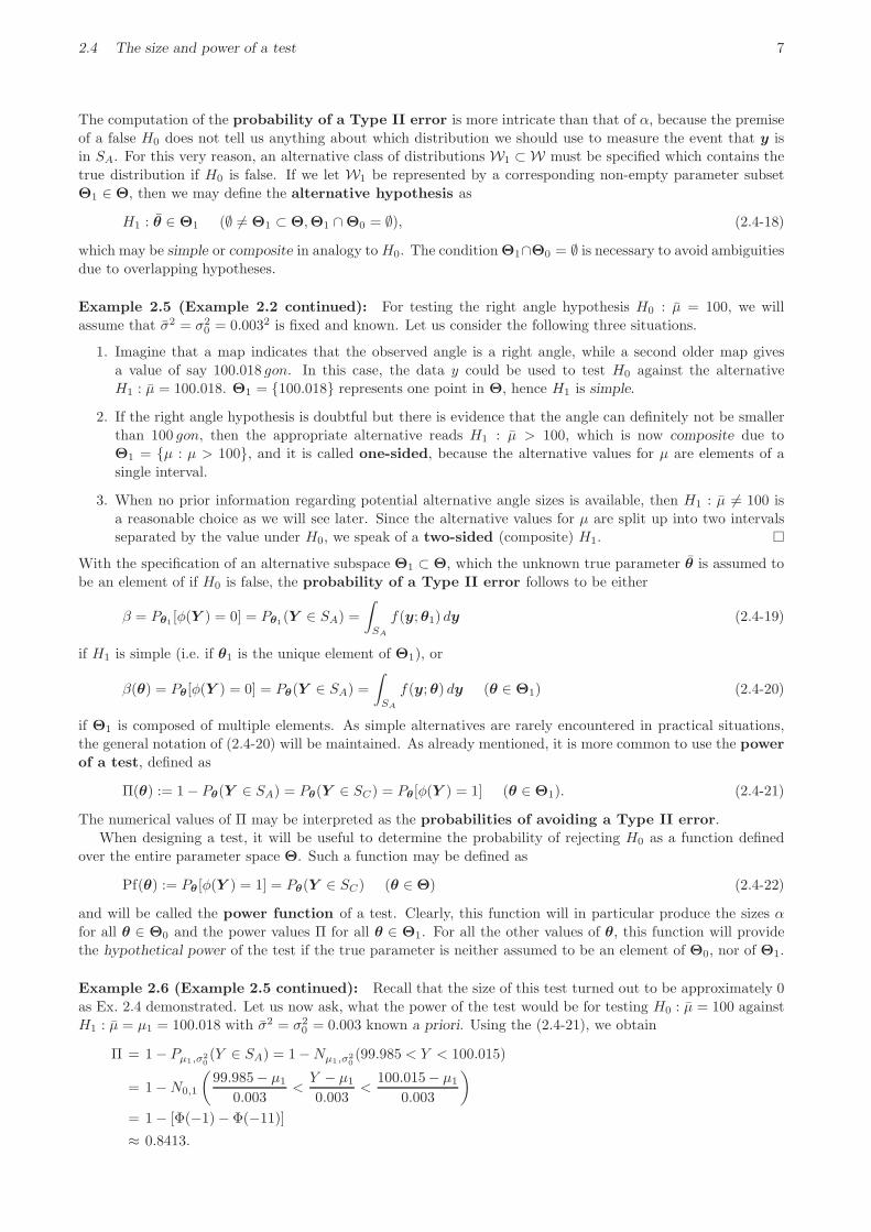
2.4 The size and power of a test 7
The computation of the probability of a Type II error is more intricate than that of α, because the premiseof a false H0 does not tell us anything about which distribution we should use to measure the event that y isin SA. For this very reason, an alternative class of distributions W1 ⊂ W must be specified which contains thetrue distribution if H0 is false. If we let W1 be represented by a corresponding non-empty parameter subsetΘ1 ∈ Θ, then we may define the alternative hypothesis as
H1 : θ ∈ Θ1 (∅ �= Θ1 ⊂ Θ,Θ1 ∩ Θ0 = ∅), (2.4-18)
which may be simple or composite in analogy to H0. The condition Θ1∩Θ0 = ∅ is necessary to avoid ambiguitiesdue to overlapping hypotheses.
Example 2.5 (Example 2.2 continued): For testing the right angle hypothesis H0 : µ = 100, we willassume that σ2 = σ2
0 = 0.0032 is fixed and known. Let us consider the following three situations.
1. Imagine that a map indicates that the observed angle is a right angle, while a second older map givesa value of say 100.018 gon. In this case, the data y could be used to test H0 against the alternativeH1 : µ = 100.018. Θ1 = {100.018} represents one point in Θ, hence H1 is simple.
2. If the right angle hypothesis is doubtful but there is evidence that the angle can definitely not be smallerthan 100 gon, then the appropriate alternative reads H1 : µ > 100, which is now composite due toΘ1 = {µ : µ > 100}, and it is called one-sided, because the alternative values for µ are elements of asingle interval.
3. When no prior information regarding potential alternative angle sizes is available, then H1 : µ �= 100 isa reasonable choice as we will see later. Since the alternative values for µ are split up into two intervalsseparated by the value under H0, we speak of a two-sided (composite) H1. �
With the specification of an alternative subspace Θ1 ⊂ Θ, which the unknown true parameter θ is assumed tobe an element of if H0 is false, the probability of a Type II error follows to be either
β = Pθ1 [φ(Y ) = 0] = Pθ1(Y ∈ SA) =∫
SA
f(y; θ1) dy (2.4-19)
if H1 is simple (i.e. if θ1 is the unique element of Θ1), or
β(θ) = Pθ[φ(Y ) = 0] = Pθ(Y ∈ SA) =∫
SA
f(y; θ) dy (θ ∈ Θ1) (2.4-20)
if Θ1 is composed of multiple elements. As simple alternatives are rarely encountered in practical situations,the general notation of (2.4-20) will be maintained. As already mentioned, it is more common to use the powerof a test, defined as
Π(θ) := 1 − Pθ(Y ∈ SA) = Pθ(Y ∈ SC) = Pθ[φ(Y ) = 1] (θ ∈ Θ1). (2.4-21)
The numerical values of Π may be interpreted as the probabilities of avoiding a Type II error.When designing a test, it will be useful to determine the probability of rejecting H0 as a function defined
over the entire parameter space Θ. Such a function may be defined as
Pf(θ) := Pθ [φ(Y ) = 1] = Pθ(Y ∈ SC) (θ ∈ Θ) (2.4-22)
and will be called the power function of a test. Clearly, this function will in particular produce the sizes α
for all θ ∈ Θ0 and the power values Π for all θ ∈ Θ1. For all the other values of θ, this function will providethe hypothetical power of the test if the true parameter is neither assumed to be an element of Θ0, nor of Θ1.
Example 2.6 (Example 2.5 continued): Recall that the size of this test turned out to be approximately 0as Ex. 2.4 demonstrated. Let us now ask, what the power of the test would be for testing H0 : µ = 100 againstH1 : µ = µ1 = 100.018 with σ2 = σ2
0 = 0.003 known a priori. Using the (2.4-21), we obtain
Π = 1 − Pµ1,σ20(Y ∈ SA) = 1 − Nµ1,σ2
0(99.985 < Y < 100.015)
= 1 − N0,1
(99.985− µ1
0.003<
Y − µ1
0.003<
100.015− µ1
0.003
)= 1 − [Φ(−1) − Φ(−11)]
≈ 0.8413.

8 2 THEORY OF HYPOTHESIS TESTING
Notice that the larger the difference between µ1 and µ0, the larger the power becomes. For instance,if H1 had been specified as µ1 = 100.021, then the power would increase to Π ≈ 0.9772, and for µ1 = 100.024the power would already be very close to 1. This is intuitively understandable, because very similar hypothesesare expected to be harder to separate on the basis of some observed data than extremely different hypotheses.Figure 2.2 illustrates this point. �
N(µ0,σ
02) → ← N(µ
1,σ
02)
← SA
SC
→
µ0
µ1
β α
← SA
SC
→
N(µ0,σ
02) → ← N(µ
1,σ
02)
µ0 µ
1
α
β
Fig. 2.2 The probability of a Type II error (β = 1−Π) becomes smaller as the distance µ1 −µ0 (with identicalvariance σ2
0) between the null hypothesis H0 and the alternative H1 increases.
Another important observation to make in this context is that, unfortunately, the errors of the first and
second kind cannot be minimized independently. For instance, when the critical region SC is extendedtowards µ0 (Fig. 2.3 left → right), then clearly its size becomes larger. In doing this, SA shrinks, and theerror of the second kind becomes smaller. This effect is explained by the fact that both errors are measuredin complementary regions and thereby affect each other’s size. Therefore, no critical function can exist thatminimizes both error probabilities simultaneously. The purpose of the following subsection is to present apractical solution to resolve this conflict.
N(µ0,σ
02) → ← N(µ
1,σ
02)
← SA
SC
→
µ0
µ1
β α
N(µ0,σ
02) → ← N(µ
1,σ
02)
← SA
SC
→
β α
Fig. 2.3 Let N(µ0, σ20) and N(µ1, σ
20) denote the distributions of a single observation Y under simple H0 and
H1, respectively. Changing the SC/SA partitioning of the observation space (abscissa) necessarily causes anincrease in probability of one error type and a decrease in probability of the other type.

2.5 Best critical regions 9
2.5 Best critical regions
As pointed out in the previous section, shifting the critical region and making one error type more unlikelyalways causes the other error to become more probable. Therefore, the probabilities of Type I and Type IIerrors cannot be minimized simultaneously. One way to resolve this conflict is to keep the probability of a TypeI error fixed at a relatively small value and to seek a critical region that minimizes the probability of a Type IIerror, or equivalently that maximizes the power of the test.
To make the mathematical concepts, necessary for this procedure, intuitively understandable, exampleswill be given mainly with respect to the class of observation models (2.1-6) introduced in Example 2.1. Theremainder of this Section 2.5 is organized such that tests with best critical regions will be constructed fortesting problems that are progressively complex within that class of models. The determination of optimalcritical regions in the context of the general linear model (2.1-1) with general parametric densities as in (2.1-3)will be subject of detailed investigations in Sections 3 and 4.
2.5.1 Most powerful (MP) tests
The simplest kind of problem for which a critical region with optimal power may exist is that of testing a simpleH0 : θ = θ0 against a simple alternative hypothesis H1 : θ = θ1 involving a single unknown parameter. Usingdefinitions (2.4-16) and (2.4-21), the problem is to find a set SC such that the restriction∫
SC
f(y; θ0) dy = α (2.5-23)
is satisfied, where α as a given size is also called the (significance) level, and∫SC
f(y; θ1)dy is a maximum. (2.5-24)
Such a critical region will be called the best critical region (BCR), and a test based on the BCR will bedenoted as most powerful (MP) for testing H0 against H1 at level α. A solution to this problem may befound on the basis of the following lemma of Neyman and Pearson (see, for instance, Rao, 1973, p. 446).
Theorem 2.1 (Neyman-Pearson Lemma). Suppose that f(Y ; θ0) and f(Y ; θ1) are two densities defined ona space S. Let SC ⊂ S be any critical region with∫
SC
f(y; θ0) dy = α, (2.5-25)
where α has a given value. If there exists a constant kα such that for the region S∗C ⊂ S with⎧⎪⎨⎪⎩
f(y; θ1)f(y; θ0)
> kα if y ∈ S∗C
f(y; θ1)f(y; θ0)
< kα if y /∈ S∗C ,
(2.5-26)
condition (2.5-25) is satisfied, then∫S∗
C
f(y; θ1)dy ≥∫
SC
f(y; θ1)dy. (2.5-27)
Notice if when f(Y ; θ0) and f(Y ; θ1) are densities under simple hypotheses H0 and H1, and if the conditions(2.5-25) and (2.5-26) hold for some kα, then S∗
C denotes the BCR for testing H0 versus H1 at fixed level α,because (2.5-27) is equivalent to the desired maximum power condition (2.5-24). Also observe that (2.5-26)then defines the MP test, which may be written as
φ(y) =
⎧⎪⎨⎪⎩1 if f(y; θ1)
f(y; θ0)> kα
0 if f(y; θ1)f(y; θ0)
< kα.(2.5-28)
This condition (2.5-28) expresses that in order for a test to be most powerful, the critical region SC mustcomprise all the observations y, for which the so-called density ratio f(y; θ1)/f(y; θ0) is larger than some

10 2 THEORY OF HYPOTHESIS TESTING
α-dependent number kα. This can be explained by the following intuitions of Stuart et al. (1999, p. 176). Usingdefinition (2.4-21), the power may be rewritten in terms of the density ratio as
Π =∫
SC
f(y; θ1) dy =∫
SC
f(y; θ1)f(y; θ0)
f(y; θ0) dy.
Since α has a fixed value, maximizing Π is equivalent to maximizing the quantity
Πα
=
∫SC
f(y; θ1)f(y; θ0)
f(y; θ0) dy∫SC
f(y; θ0) dy
.
In order for a test to have maximum power, its critical region SC must clearly include all the observations y,
1. for which the integral value in the denominator equals α, and
2. for which the density ratio in the nominator produces the largest possible values, whose lower bound maybe defined as the number kα (with the values of the additional factor f(y; θ0) fixed by condition 1).
These are the very conditions given by the Neyman-Pearson Lemma. A more formal proof may be found, forinstance, in Teunissen (2000, p. 30f.). The following example demonstrates how the BCR may be constructedfor a simple test problem by applying the Neyman-Pearson Lemma.
Example 2.7: Test of the normal mean with known variance - Simple alternatives. Let Y1, . . . , Yn
be independently and normally distributed observations with common unknown mean µ and common knownstandard deviation σ = σ0. What is the BCR for a test of the simple null hypothesis H0 : µ = µ0 against thesimple alternative hypothesis H1 : µ = µ1 at level α? (It is assumed that µ0, µ1, σ0 and α have fixed numericalvalues.)
In order to construct the BCR, we will first try to find a number kα such that condition (2.5-26) about thedensity ratio f(y; θ1)/f(y; θ0) holds. As the observations are independently distributed with common mean µ
and variance σ20 , the factorized form of the joint normal density function f(y) according to Example 2.1 may
be applied. This yields the expression
f(y; θ1)f(y; θ0)
=
n∏i=1
1√2πσ0
exp
{−1
2
(yi − µ1
σ0
)2}
n∏i=1
1√2πσ0
exp
{−1
2
(yi − µ0
σ0
)2} =
(1√
2πσ0
)n
exp
{− 1
2σ20
n∑i=1
(yi − µ1)2}
(1√
2πσ0
)n
exp
{− 1
2σ20
n∑i=1
(yi − µ0)2} (2.5-29)
for the density ratio. An application of the ordinary binomial formula allows us to split off a factor that doesnot depend on µ, that is
f(y; θ1)f(y; θ0)
=
(1√
2πσ0
)n
exp
{− 1
2σ20
n∑i=1
y2i
}exp
{− 1
2σ20
n∑i=1
(−2yiµ1 + µ21)
}(
1√2πσ0
)n
exp
{− 1
2σ20
n∑i=1
y2i
}exp
{− 1
2σ20
n∑i=1
(−2yiµ0 + µ20)
} . (2.5-30)
Now, the first two factors in the nominator and denominator cancel out due to their independence of µ.Rearranging the remaining terms leads to
f(y; θ1)f(y; θ0)
=
exp
{µ1
σ20
n∑i=1
yi − nµ21
2σ20
}
exp
{µ0
σ20
n∑i=1
yi − nµ20
2σ20
} (2.5-31)
= exp
{µ1
σ20
n∑i=1
yi − µ0
σ20
n∑i=1
yi − nµ21
2σ20
+nµ2
0
2σ20
}(2.5-32)
= exp
{1σ2
0
(µ1 − µ0)n∑
i=1
yi − n
2σ20
(µ21 − µ2
0)
}, (2.5-33)

2.5 Best critical regions 11
which reveals two remarkable facts: the simplified density ratio depends on the observations only through theirsum
∑ni=1 yi, and the density ratio, as an exponential function, is a positive number. Therefore, we may choose
another positive number kα such that
exp
{1σ2
0
(µ1 − µ0)n∑
i=1
yi − n
2σ20
(µ21 − µ2
0)
}> kα (2.5-34)
always holds. Taking natural logarithms on both sides of this inequality yields
1σ2
0
(µ1 − µ0)n∑
i=1
yi − n
2σ20
(µ21 − µ2
0) > ln kα
or, after multiplication with 2σ20 and expansion of the left side by n · 1
n ,
2n(µ1 − µ0)1n
n∑i=1
yi > 2σ20 ln kα + n(µ2
1 − µ20).
Depending on whether µ1 > µ0 or µ1 < µ0, the sample mean y = 1n
∑ni=1 yi must satisfy
y >2σ2
0 ln kα + n(µ21 − µ2
0)2n(µ1 − µ0)
=: k′α (if µ1 > µ0)
or
y <2σ2
0 ln kα + n(µ21 − µ2
0)2n(µ1 − µ0)
=: k′α (if µ1 < µ0)
in order for the second condition (2.5-26) of the Neyman-Pearson Lemma to hold. Note that the quantitiesσ2
0 , n, µ1, µ0 are all constants fixed a priori, and kα is a constant whose exact value is still to be determined.Thus, k′
α is itself an unknown constant.Now, in order for the first condition (2.5-25) of the Neyman-Pearson Lemma to hold in addition, SC must
have size α under the null hypothesis. As mentioned above, the critical region SC may be constructed solely byinspecting the value y, which may be viewed as the outcome of the random variable Y := 1
n
∑ni=1 Yi. Under H0,
Y is normally distributed with expectation µ0 (identical to the expectation of each of the original observationsY1, . . . , Yn) and standard deviation σ0/
√n. Therefore, the size is determined by
α =
⎧⎨⎩Nµ0,σ20/n(Y > k′
α) if µ1 > µ0,
Nµ0,σ20/n(Y < k′
α) if µ1 < µ0.
It will be more convenient to standardize Y because this allows us to evaluate the size in terms of the standardnormal distribution. The condition to be satisfied by k′
α then reads
α =
⎧⎪⎪⎨⎪⎪⎩N0,1
(Y − µ0
σ0/√
n>
k′α − µ0
σ0/√
n
)if µ1 > µ0,
N0,1
(Y − µ0
σ0/√
n<
k′α − µ0
σ0/√
n
)if µ1 < µ0,
or, using the standard normal distribution function Φ,
α =
⎧⎪⎪⎨⎪⎪⎩1 − Φ
(k′
α − µ0
σ0/√
n
)if µ1 > µ0,
Φ(
k′α − µ0
σ0/√
n
)if µ1 < µ0.
Rewriting this as
Φ(
k′α − µ0
σ0/√
n
)=
⎧⎨⎩ 1 − α if µ1 > µ0,
α if µ1 < µ0

12 2 THEORY OF HYPOTHESIS TESTING
allows us to determine the argument of Φ by applying the inverse standard normal distribution function Φ−1
to the previous equation, which yields
k′α − µ0
σ0/√
n=
⎧⎨⎩Φ−1(1 − α) if µ1 > µ0,
Φ−1(α) if µ1 < µ0,
from which the constant k′α is obtained as
k′α =
⎧⎪⎨⎪⎩µ0 + σ0√
nΦ−1(1 − α) if µ1 > µ0,
µ0 + σ0√n
Φ−1(α) if µ1 < µ0,
or
k′α =
⎧⎪⎨⎪⎩µ0 + σ0√
nΦ−1(1 − α) if µ1 > µ0,
µ0 − σ0√n
Φ−1(1 − α) if µ1 < µ0.
Consequently, depending on the sign of µ1 − µ0, there are two different values for k′α that satisfy the first
condition (2.5-25) of the Neyman-Pearson Lemma. When µ1 > µ0 the BCR is seen to consist of all theobservations y ∈ S, for which
y > µ0 +σ0√n
Φ−1(1 − α), (2.5-35)
and when µ1 < µ0, the BCR reads
y < µ0 − σ0√n
Φ−1(1 − α). (2.5-36)
In the first case (µ1 > µ0), the MP test is given by
φu(y) =
⎧⎪⎨⎪⎩1 if y > µ0 + σ0√
nΦ−1(1 − α),
0 if y < µ0 + σ0√n
Φ−1(1 − α),(2.5-37)
and in the second case (µ1 < µ0), the MP test is
φl(y) =
⎧⎪⎨⎪⎩1 if y < µ0 − σ0√
nΦ−1(1 − α),
0 if y > µ0 − σ0√n
Φ−1(1 − α).(2.5-38)
Observe that the critical regions depend solely on the value of the one-dimensional random variable Y , which,as a function of the observations Y , is also called a statistic. As this statistic appears in the specific context ofhypothesis testing, we will speak of Y as a test statistic. We see from this that it is not necessary to actuallyspecify an n-dimensional region SC used as the BCR, but the BCR may be expressed conveniently in terms ofone-dimensional intervals. For this purpose, let (cu, +∞) and (−∞, cl) denote the critical regions with respectto the sample mean y as defined by (2.5-35) and (2.5-36). The real constants
cu := µ0 +σ0√n
Φ−1(1 − α) (2.5-39)
and
cl := µ0 − σ0√n
Φ−1(1 − α) (2.5-40)
are called the upper critical value and the lower critical value corresponding to the BCR for testing H0
versus H1.In a practical situation, it will be clear from the numerical specification of H1 which of the tests (2.5-37)
and (2.5-38) should be applied. Then, the test is carried out by computing the mean y of the given data y andby checking how large its value is in comparison to the critical value of (2.5-37) or (2.5-38), respectively. �

2.5 Best critical regions 13
Example 2.8: A most powerful test about the Beta distribution. Let Y1, . . . , Yn be independentlyand B(α, β)-distributed observations on [0, 1] with common unknown parameter α (which in this case is not tobe confused with the size or level of the test) and common known parameter β = 1 (not to be confused withthe probability of a Type II error). What is the BCR for a test of the simple null hypothesis H0 : α = α0 = 1against the simple alternative hypothesis H1 : α = α1 = 2 at level α∗?
The density function of the univariate Beta distribution in standard form is defined by
f(y; α, β) =Γ(α + β)Γ(α)Γ(β)
yα−1(1 − y)β−1 (0 < y < 1; α, β > 0), (2.5-41)
see Johnson and Kotz (1970b, p. 37) or Koch (1999, p. 115). Notice that (2.5-41) simplifies under H0 to
f(y; α0) =Γ(2)
Γ(1)Γ(1)y1−1(1 − y)1−1 = 1 (0 < y < 1), (2.5-42)
and under H1 to
f(y; α1) =Γ(3)
Γ(2)Γ(1)y2−1(1 − y)1−1 = 2y (0 < y < 1) (2.5-43)
where we used the facts that Γ(1) = Γ(2) = 1 and Γ(3) = 2. The density 2.5-42 defines the so-called uniformdistribution with parameters a = 0 and b = 1, see Johnson and Kotz (1970b, p. 57) or Koch (2000, p. 21). Wemay now proceed as in Example 2.7 and determine the BCR by using the Neyman-Pearson Lemma (Theorem2.1). For n independent observations, the joint density may be written as the product of the individual univariatedensities, which results in the density ratio
f(y; α1)f(y; α0)
=n∏
i=1
2yi/n∏
i=1
1 = 2nn∏
i=1
yi, (2.5-44)
where we assumed that each observation is strictly within the interval (0, 1). As the density ratio is a positivenumber, we may choose a number kα∗ such that 2n
∏ni=1 yi > kα∗ holds. Division by 2n and taking both sides
to the power of 1/n yields the equivalent inequality(n∏
i=1
yi
)1/n
>(2−nkα∗
)1/n.
Now we have found a seemingly convenient condition about the sample’s geometric mean Y := (∏n
i=1 Yi)1/n
rather than about the entire sample Y itself. Then the second condition (2.5-26 or equivalently 2.5-28) of theNeyman-Pearson Lemma gives
φ(y) =
⎧⎨⎩ 1 if y > (2−nkα∗)1/n =: k′α∗
0 if y < (2−nkα∗)1/n =: k′α∗ .
To ensure that φ has some specified level α∗, the first condition (2.5-25) of the Neyman-Pearson Lemma requiresthat α∗ equals the probability under H0 that the geometric mean exceeds k′
α∗ . Unfortunately, in contrast tothe arithmetic mean Y of n independent normal variables, the geometric mean Y of n independent standarduniform variables does not have a standard distribution. However, as Stuart and Ord (2003, p. 393) demonstratein their Example 11.15, the statistic
U := − ln Y n = − lnn∏
i=1
Yi = −n∑
i=1
ln Yi
follows a Gamma distribution G(b, p) with b = 1 and p = n, defined by Equation 2.107 in Koch (1999, p. 112).Thus the first Neyman-Pearson condition reads
α∗ = G1,n(U > k′′α∗) = 1 − FG1,n(k′′
α∗),
from which the critical value k′′α∗ follows to be k′′
α∗ = F−1G1,n
(1 − α∗), and which may be obtained in MATLABby executing the command CV = gaminv(1− α∗, n, 1). In summary, the MP test is given by
φ(y) =
⎧⎪⎪⎨⎪⎪⎩1 if u(y) = −
n∑i=1
ln yi > k′′α∗ = − ln (2−nkα∗) = F−1
G1,n(1 − α∗),
0 if u(y) = −n∑
i=1
ln yi < k′′α∗ = − ln (2−nkα∗) = F−1
G1,n(1 − α∗).
�

14 2 THEORY OF HYPOTHESIS TESTING
2.5.2 Reduction to sufficient statistics
We saw in Example 2.7 that applying the conditions of the Neyman-Pearson Lemma to derive the BCR led to acondition about the sample mean y rather than about the original data y. We might say that it was sufficientto use the mean value of the data for testing a hypothesis about the parameter µ of the normal distribution.This raises the important question of whether it is always possible to reduce the data in such a way.
To generalize this idea, let F = {f(y; θ) : θ ∈ Θ} be a collection of densities where the parameter θ isunknown. Further, let each f(y; θ) depend on the value of a random function or statistic T (Y ) which isindependent of θ. If any inference about θ, be it estimation or testing, depends on the observations Y onlythrough the value of T (Y ), then this statistic will be called sufficient for θ.
This qualitative definition of sufficiency can be interpreted such that a sufficient statistic captures all therelevant information that the data contains about the unknown parameters. The point is that the data mighthave some additional information that does not contribute anything to solving the estimation or test problem.The following classical example highlights this distinction between information that is essential and informationthat is completely negligible for estimating an unknown parameter.
Example 2.9: Sufficient statistic in Bernoulli’s random experiment. Let Y1, . . . , Yn denote inde-pendent binary observations within an idealized setting of Bernoulli’s random experiment (see, for instance,Lehmann, 1959a, p. 17-18). The probability p of the elementary event success (yi = 1) is assumed to be un-known, but valid for all observations. The probability of the second possible outcome failure (yi = 0) is then1 − p.
Now, it is intuitively clear that in order to estimate the unknown success rate p, it is completely sufficientto know how many successes T (y) :=
∑ni=1 yi occurred in total within n trials. The additional information
regarding which specific observations were successes or failures does not contribute anything useful for deter-mining the success rate p. In this sense the use of the statistic T (Y ) reduces the n data to a single value whichcarries all the essential information required to determine p. �
The concept of sufficiency provides a convenient tool to achieve a data reduction without any loss of informationabout the unknown parameters. The definition above, however, is not easily applicable when one has to dealwith specific estimation or testing problems. As a remedy, Neyman’s Factorization Theorem gives aneasy-to-check condition for the existence of a sufficient statistic in any given parametric inference problem.
Theorem 2.2 (Neyman’s Factorization Theorem). Let F = {f(y; θ) : θ ∈ Θ} be a collection of densities fora sample Y = (Y1, . . . , Yn). A vector of statistics T (Y ) is sufficient for θ if and only if there exist functionsg(T (Y ); θ) and h(Y ) such that
f(y; θ) = g(T (y); θ) · h(y) (2.5-45)
holds for all θ ∈ Θ and all y ∈ S.
Proof. A deeper understanding of the sufficiency concept involves an investigation into conditional probabilitieswhich is beyond the scope of this thesis. The reader familiar with conditional probabilities is referred to Lehmannand Romano (2005, p. 20) for a proof of this theorem.
It is easy to see that the trivial choice T (y) := y, g(T (y); θ) := f(y; θ) and h(y) := 1 is always possible, butachieves no data reduction. Far more useful is the fact that any reversible function of a sufficient statistic isalso sufficient for θ (cf. Casella and Berger, 2002, p. 280). In particular, multiplying a sufficient statistic withconstants yields again a sufficient statistic. The following example will now establish sufficient statistics for thenormal density with both parameters µ and σ2 unknown.
Example 2.10: Suppose that observations Y1, . . . , Yn are independently and normally distributed with com-mon unknown mean µ and common unknown variance σ2. Let the sample mean and variance be defined asY =
∑ni=1 Yi/n and S2 =
∑ni=1(Yi − Y )2/(n−1), respectively. The joint normal density can then be written as
f(y; µ, σ2) =n∏
i=1
1√2πσ
exp{− 1
2σ2(yi − µ)2
}= (2πσ2)−n/2 exp
{−nµ2
2σ2+
µ
σ2
n∑i=1
yi − 12σ2
n∑i=1
y2i
}
= (2πσ2)−n/2 exp{− n
2σ2(y − µ)2 − n − 1
2σ2s2
}· IRn(y)
where T (Y ) := [ Y , S2 ]′ is sufficient for (µ, σ2) and h(y) := IRn(y) = 1 with I as the indicator function. �
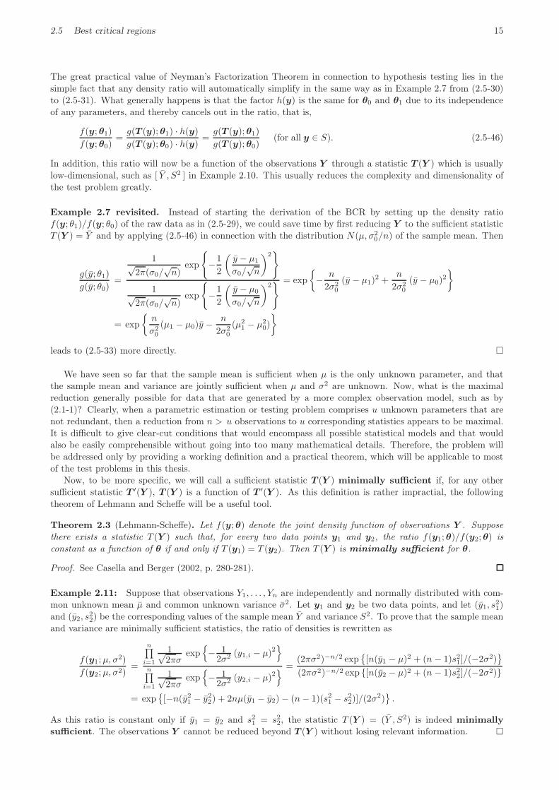
2.5 Best critical regions 15
The great practical value of Neyman’s Factorization Theorem in connection to hypothesis testing lies in thesimple fact that any density ratio will automatically simplify in the same way as in Example 2.7 from (2.5-30)to (2.5-31). What generally happens is that the factor h(y) is the same for θ0 and θ1 due to its independenceof any parameters, and thereby cancels out in the ratio, that is,
f(y; θ1)f(y; θ0)
=g(T (y); θ1) · h(y)g(T (y); θ0) · h(y)
=g(T (y); θ1)g(T (y); θ0)
(for all y ∈ S). (2.5-46)
In addition, this ratio will now be a function of the observations Y through a statistic T (Y ) which is usuallylow-dimensional, such as [ Y , S2 ] in Example 2.10. This usually reduces the complexity and dimensionality ofthe test problem greatly.
Example 2.7 revisited. Instead of starting the derivation of the BCR by setting up the density ratiof(y; θ1)/f(y; θ0) of the raw data as in (2.5-29), we could save time by first reducing Y to the sufficient statisticT (Y ) = Y and by applying (2.5-46) in connection with the distribution N(µ, σ2
0/n) of the sample mean. Then
g(y; θ1)g(y; θ0)
=
1√2π(σ0/
√n)
exp
{−1
2
(y − µ1
σ0/√
n
)2}
1√2π(σ0/
√n)
exp
{−1
2
(y − µ0
σ0/√
n
)2} = exp
{− n
2σ20
(y − µ1)2 +n
2σ20
(y − µ0)2}
= exp{
n
σ20
(µ1 − µ0)y − n
2σ20
(µ21 − µ2
0)}
leads to (2.5-33) more directly. �
We have seen so far that the sample mean is sufficient when µ is the only unknown parameter, and thatthe sample mean and variance are jointly sufficient when µ and σ2 are unknown. Now, what is the maximalreduction generally possible for data that are generated by a more complex observation model, such as by(2.1-1)? Clearly, when a parametric estimation or testing problem comprises u unknown parameters that arenot redundant, then a reduction from n > u observations to u corresponding statistics appears to be maximal.It is difficult to give clear-cut conditions that would encompass all possible statistical models and that wouldalso be easily comprehensible without going into too many mathematical details. Therefore, the problem willbe addressed only by providing a working definition and a practical theorem, which will be applicable to mostof the test problems in this thesis.
Now, to be more specific, we will call a sufficient statistic T (Y ) minimally sufficient if, for any othersufficient statistic T ′(Y ), T (Y ) is a function of T ′(Y ). As this definition is rather impractial, the followingtheorem of Lehmann and Scheffe will be a useful tool.
Theorem 2.3 (Lehmann-Scheffe). Let f(y; θ) denote the joint density function of observations Y . Supposethere exists a statistic T (Y ) such that, for every two data points y1 and y2, the ratio f(y1; θ)/f(y2; θ) isconstant as a function of θ if and only if T (y1) = T (y2). Then T (Y ) is minimally sufficient for θ.
Proof. See Casella and Berger (2002, p. 280-281).
Example 2.11: Suppose that observations Y1, . . . , Yn are independently and normally distributed with com-mon unknown mean µ and common unknown variance σ2. Let y1 and y2 be two data points, and let (y1, s
21)
and (y2, s22) be the corresponding values of the sample mean Y and variance S2. To prove that the sample mean
and variance are minimally sufficient statistics, the ratio of densities is rewritten as
f(y1; µ, σ2)f(y2; µ, σ2)
=
n∏i=1
1√2πσ
exp{− 1
2σ2 (y1,i − µ)2}
n∏i=1
1√2πσ
exp{− 1
2σ2 (y2,i − µ)2} =
(2πσ2)−n/2 exp{[n(y1 − µ)2 + (n − 1)s2
1]/(−2σ2)}
(2πσ2)−n/2 exp {[n(y2 − µ)2 + (n − 1)s22]/(−2σ2)}
= exp{[−n(y2
1 − y22) + 2nµ(y1 − y2) − (n − 1)(s2
1 − s22)]/(2σ2)
}.
As this ratio is constant only if y1 = y2 and s21 = s2
2, the statistic T (Y ) = (Y , S2) is indeed minimallysufficient. The observations Y cannot be reduced beyond T (Y ) without losing relevant information. �

16 2 THEORY OF HYPOTHESIS TESTING
2.5.3 Uniformly most powerful (UMP) tests
The concept of the BCR for testing a simple H0 against a simple H1 about a single parameter, as defined by theNeyman-Pearson Lemma, is dissatifactory insofar that the great majority of test problems involves compositealternatives. The question to be addressed in this subsection is how a BCR may be defined for such problems.
Let us start with the basic premise that we seek an optimal critical function for testing the simple null
H0 : θ = θ0 (2.5-47)
versus a composite alternative hypothesis
H1 : θ ∈ Θ1, (2.5-48)
where the set of parameter values Θ1 and θ0 are disjoint subsets of a one-dimensional parameter space Θ. Themost straightforward way to establish optimality under these conditions is to determine the BCR for testingH0 against a fixed simple H1 : θ = θ1 for an arbitrary θ1 ∈ Θ1 and to check whether the resulting BCR isindependent of the specific value θ1. If this is the case, then all the values θ1 ∈ Θ1 produce the same BCR,because θ1 was selected arbitrarily. This critical region that all the simple alternatives H ′
1 in
H1 = {H ′1 : θ = θ1 with θ1 ∈ Θ1} (2.5-49)
have in common may then be defined as the BCR for testing a simple H0 against a composite H1. Atest based on such a BCR is called uniformly most powerful (UMP) for testing H0 versus H1 at level α.
Now, it seems rather cumbersome to derive the BCR for a composite H1 by applying the conditions of theNeyman-Pearson Lemma to each simple H ′
1 ∈ H1. The following theorem replaces this infeasible procedureby conditions that can be verified more directly. These conditions say that in order for a UMP test to exist,(1) the test problem may have only one unknown parameter , (2) the alternative hypothesis must be one-sided , and (3) each distribution in W must have a so-called monotone density ratio . The third conditionmeans that, for all θ1 > θ0 with θ0, θ1 ∈ Θ, the ratio f(y; θ1)/f(y; θ0) (or the ratio g(t; θ1)/g(t; θ0) in termsof the sufficient statistic T (Y )) must be a strictly monotonical function of T (Y ). The following example willilluminate this issue.
Example 2.12: To show that the normal distribution N(µ, σ20) with unknown µ and known σ2
0 has a monotonedensity ratio, we may directly inspect the simplified density ratio (2.5-33) from Example 2.7. We see immediatelythat the ratio is an increasing function of T (y) :=
∑ni=1 yi when µ1 > µ0. �
Theorem 2.4. Let W be a class of distributions with a one-dimensional parameter space and monotone densityratio in some statistic T (Y ).
1. Suppose that H0 : θ = θ0 is to be tested against the upper one-sided alternative H1 : θ > θ0. Then,there exists a UMP test φu at level α and a constant C with
φu(T (y)) :=
⎧⎨⎩ 1, if T (y) > C,
0, if T (y) < C(2.5-50)
and
Pθ0 {φu(T (Y )) = 1} = α. (2.5-51)
2. For testing H0 against the lower one-sided alternative H1 : θ < θ0, there exists a UMP test φl at levelα and a constant C with
φl(T (y)) :=
⎧⎨⎩ 1, if T (y) < C
0, if T (y) > C(2.5-52)
and
Pθ0 {φl(T (Y )) = 1} = α. (2.5-53)

2.5 Best critical regions 17
Proof. To prove (1), consider first the case of a simple alternative H1 : θ = θ1 for some θ1 > θ0. With the valuesfor θ0 and θ1 fixed, the density ratio can be written as
f(y; θ1)f(y; θ0)
=g(T (y); θ1)g(T (y); θ0)
= h(T (y)),
that is, as a function of the observations alone. According to the Neyman-Pearson Lemma 2.1, the ratio mustbe large enough, i.e. h(T (y)) > k with k depending on α. Now, if T (y1) < T (y2) holds for some y1, y2 ∈ S,then certainly also h(T (y1)) ≤ h(T (y2)) due to the assumption that the density ratio is monotone in T ((Y )).In other words, the observation y2 is in both cases at least as suitable as y1 for making the ratio h sufficientlylarge. In this way, the BCR may be equally well constructed by all the data y ∈ S for which T (y) is largeenough, for instance T (y) > C, where the constant C must be determined such that the size of this BCR equalsthe prescribed value α. As these implications are true regardless of the exact value θ1, the BCR will be thesame for all the simple alternatives with θ1 > θ0. Therefore, the test (2.5-50) is UMP. The proof of (2) followsthe same sequence of arguments with all inequalities reversed.
The next theorem is of great practical value as it ensures that most of the standard distributions used inhypothesis testing have a monotone density ratio even in their non-central forms.
Theorem 2.5. The following 1P -distributions (with possibly additional known parameters µ0, σ20 , p0 and known
degrees of freedom f0, f1,0, f2,0) have a density with monotone density ratio in some statistic T :
1. Multivariate independent normal distributions N(1µ, σ20I) and N(1µ0, σ
2I),
2. Gamma distribution G(b, p0),
3. Beta distribution B(α, β0),
4. Non-central Student distribution t(f0, λ),
5. Non-central Chi-squared distribution χ2(f0, λ),
6. Non-central Fisher distribution F (f1,0, f2,0, λ),
Proof. The proofs of (1) and (2) may be elegantly based on the more general result that any density that is amember of the one-parameter exponential family, defined by
f(y; θ) = h(y)c(θ) exp {w(θ)T (y)} , h(y) ≥ 0, c(θ) ≥ 0, (2.5-54)
(cf. Olive, 2006, for more details) has a monotone density ratio (see Lehmann and Romano, 2005, p. 67), andthat the normal and Gamma distributions can be written in this form (2.5-54).
1. The density function of N(1µ, σ20I) (2.5-29) can be rewritten as
f(y; µ) = (2πσ20)−n/2 exp
{− 1
2σ20
n∑i=1
y2i
}exp{−nµ2
2σ20
}exp
{µ
σ20
n∑i=1
yi
},
where h(y) := (2πσ20)−n/2 exp
{− 1
2σ20
∑ni=1 y2
i
}≥ 0, c(θ) := exp{−nµ2
2σ20} ≥ 0, w(θ) := µ
σ20, and T (y) :=∑n
i=1 yi satisfy (2.5-54). Similarly, the density function of N(1µ0, σ2I) reads, in terms of (2.5-54),
f(y; σ2) = IRn(y)(2πσ2)−n/2 exp
{− 1
2σ2
n∑i=1
(yi − µ0)2}
,
where h(y) corresponds to the indicator function IRn(y) with definite value one, c(θ) := (2πσ2)−n/2 ≥ 0,w(θ) := − 1
2σ2 , and T (y) :=∑n
i=1(yi − µ0)2.
2. The Gamma distribution, defined by Equation 2.107 in Koch (1999, p. 112), with known parameter p0
may be directly written as
f(y; b) =yp0−1
Γ(p0)bp0 exp{−by} (b > 0, p0 > 0, y ∈ R
+),
where h(y) := yp0−1/Γ(p0) ≥ 0, c(θ) := bp0 ≥ 0, w(θ) := b, and T (y) := −y satisfy (2.5-54).
3. - 6. The proofs for these distributions are lengthy and may be obtained from Lehmann and Romano(2005, p. 224 and 307).

18 2 THEORY OF HYPOTHESIS TESTING
Example 2.13: Test of the normal mean with known variance (composite alternatives). We arenow in a position to extend Example 2.7 and seek BCRs for composite alternative hypotheses. For demonstrationpurposes, both the raw definition of a UMP test and the more convenient Theorem 2.4 will applied if possible.Let us first look at the formal statement of the test problems.
Let Y1, . . . , Yn be independently and normally distributed observations with common unknown mean µ andcommon known variance σ2 = σ2
0 . Do a UMP tests for testing the simple null hypothesis H0 : µ = µ0 againstthe composite alternative hypothesis
1. H1 : µ > µ0,
2. H1 : µ < µ0,
3. H1 : µ �= µ0
exist at level α, and if so, what are the BCRs? (It is assumed that µ0, σ0 and α have fixed numerical values.)
1. Recall from Example 2.7 (2.5-35) that the BCR for the test of H0 : µ = µ0 against the simple H1 : µ = µ1
with µ1 > µ0 is given by all the observations satisfying
y > µ0 +σ0√n
Φ−1(1 − α),
when µ1 > µ0. Evidently, the critical region is the same for all the simple alternatives
{H ′1 : µ = µ1 with µ1 > µ0} ,
because it is independent of µ1. Therefore, the critical function (2.5-37) is UMP for testing H0 against thecomposite alternative H1 : µ > µ0. The following alternative proof makes direct use of Theorem 2.4.
In Example 2.12, the normal distribution N(µ, σ20) with known variance was already demonstrated to have
a monotone density ratio in the sufficient statistic∑n
i=1 Yi or in T (Y ) :=∑n
i=1 Yi/n as a reversible functionthereof. As the current testing problem is about a single parameter, a one-sided H1, and a class of distributionwith monotone density ratio, all the conditions of Theorem 2.4 are satisfied. It remains to find a constant C
such that the critical region (2.5-50) has size α according to condition (2.5-51). It is found easily because weknow already that T (Y ) is distributed as N(µ0, σ
20) under H0, so that
α = Pµ0,σ20/n{φ(Y ) = 1} = Pµ0,σ2
0/n{Y ∈ SC} = Nµ0,σ20/n{T (Y ) > C} = 1 − N0,1
(T (Y ) − µ0
σ0/√
n<
C − µ0
σ0/√
n
)= 1 − Φ
(C − µ0
σ0/√
n
),
from which C follows to be
C = µ0 +σ0√n
Φ−1(1 − α).
Note that the number C would change to C = nµ0 +√
nσ0√
nΦ−1(1 − α) if∑n
i=1 Yi was used as the sufficientstatistic instead of
∑ni=1 Yi/n, because the mean and variance of the normal distribution are affected by the
factor 1/n.
2. The proof of existence and determination of the BCR of a UMP test for testing H0 versus H1 : µ < µ0 isanalogous to the first case above. All the conditions required by Theorem 2.4 are satisfied, and the constant C
appearing in the UMP test (2.5-52) and satisfying (2.5-53) is now found to be
C = µ0 − σ0√n
Φ−1(1 − α).
3. In this case, there is no common BCR for testing H0 against H1 : µ �= µ0. Although the BCRs (2.5-35) and(2.5-36) do not individually depend on the value of µ1, they differ in signs through the location of µ1 relativeto µ0. Consequently, there is no UMP test for the two-sided alternative. This fact is also reflected by Theorem2.4, which requires the alternative to be one-sided. �

2.5 Best critical regions 19
2.5.4 Reduction to invariant statistics
We will now tackle the problem of testing a generally multi-parameter and composite null hypothesis
H0 : θ ∈ Θ0
against a possibly composite and two-sided alternative
H1 : θ ∈ Θ1
with the usual assumption that Θ0 and Θ1 are non-empty and disjoint subsets of the parameter space Θ, whichis connected to a parametric family of densities
F = {f(y; θ) : θ ∈ Θ} ,
or equivalently
FT = {fT (T (y); θ) : θ ∈ Θ} ,
when (minimally) sufficient statistics T (Y ) are used as ersatz observations for Y . Recall that sufficiency onlyreduces the dimension of the observation space, whereas it always leaves the parameter space unchanged. Theproblem is now that no UMP test exists when the parameter space is multi-dimensional or when the alternativehypothesis is two-sided, because the conditions of Theorem 2.4 would be violated. To overcome this seriouslimitation, we will investigate a reduction technique that may be applied in addition to a reduction by sufficiency,and that will oftentimes produce a simplified test problem for which a UMP test then exists.
Since any reduction beyond minimal sufficiency is necessarily bound to cause a loss of relevant information,it is essential to understand what kind of information may be safely discarded in a given test problem, andwhat the equivalent mathematical transformation is. The following example gives a first demonstration aboutthe nature of such transformations.
Example 2.14: Recall from Example 2.13 that there exists no UMP test for testing H0 : µ = µ0 = 0 againstthe two-sided H1 : µ �= µ0 = 0 (with σ2 = σ2
0 known), as the one-sidedness condition of Theorem 2.4 is violated.However, if we discard the sign of the sample mean, i.e. if we only measure the absolute deviation of the samplemean from µ0, and if we use the sign-insensitive statistic Y 2 instead of Y , then the problem becomes one oftesting H0 : µ2 = 0 against the one-sided H1 : µ2 > 0. This is so because Y ∼ N(µ, σ2
0/n) implies that nσ20
Y 2
has a non-central chi-squared distribution χ2(1, λ) with one degree of freedom and non-centrality parameterλ = n
σ20
µ2 (see Koch, 1999, p. 127). Then, µ = 0 is equivalent to λ = 0 under H0, and µ �= 0 is equivalentto λ > 0 under H1. As the transformed test problem is about a one-sided alternative and a test statistic witha monotone density ratio (by virtue of Theorem 2.5-4), the UMP test according to (2.5-50) of Theorem 2.4 isgiven by
φ(n
σ20
y2) :=
⎧⎨⎩ 1, if nσ20
y2 > C,
0, if nσ20
y2 < C,(2.5-55)
where, according to condition (2.5-51), C is fixed such that the size of (2.5-55) equals the prescribed valueα. Using definition (2.4-16) and the fact that n
σ20
Y 2 has a central chi-squared distribution with one degree offreedom under H0, this is
α = 1 − χ21,0
(n
σ20
Y 2 < C
)= 1 − Fχ2
1,0(C) ,
which yields as the critical value
C = F−1χ2
1,0(1 − α).
We will call the transformed problem of testing H0 : λ = 0 against H1 : λ > 0 the invariance-reducedtesting problem, and the corresponding test 2.5-55 (based on Theorem 2.4) the UMP invariant test. Itwill be interesting to compare the power function of this test with the power functions of the UMP tests for

20 2 THEORY OF HYPOTHESIS TESTING
the one-sided alternatives from Example 2.13. Using (2.4-22), the power function of the invariant test (2.5-55)reads
Pf(µ) = 1 − χ21,nµ2/σ2
0
(n
σ20
Y 2 < C
)= 1 − Fχ2
1,nµ2/σ20
(F−1
χ21,0
(1 − α))
.
The power functions of the upper and lower one-sided UMP tests derived in Example 2.13 (here with the specificvalue µ0 = 0) are found to be
Pf(1)(µ) = 1 − Φ(
Φ−1(1 − α) −√
n
σ0µ
)and
Pf(2)(µ) = 1 − Φ(−Φ−1(1 − α) −
√n
σ0µ
),
respectively.
0
0.05
1
Pow
er fu
nctio
n
One−sided − left
One−sided − right
Two−sided
Fig. 2.4 Power functions for the two UMP tests at level α = 0.05 about H1 : µ < 0 (’lower one-sided’) andH1 : µ > 0 (’upper one-sided’), and a UMP invariant test about H1 : µ �= 0 reduced to H1 : µ2 > 0.
Figure 2.4 shows that each of the UMP tests has slightly higher power within their one-sided Θ1-domains thanthe invariance-reduced test for the originally two-sided alternative. Observe that each of the UMP one-sidedtests would have practically zero power when the value of the true parameter is unexpectedly on the other sideof the parameter space. On the other hand, the invariance-reduced test guarantees reasonable power throughoutthe entire two-sided parameter space.
Clearly, the power function of the invariance-reduced test (2.5-55) is symmetrical with respect to µ = 0,because the sign of the sample mean, and consequently that of the mean parameter, is not being considered.Therefore, we might say that this test has been designed to be equally sensitive in both directions awayfrom µ0 = 0. In mathematical terminology, one would say that the test is invariant under sign changesY → ±Y , and Y 2 is a sign-invariant statistic, i.e. a random variable whose value remains unchanged whenthe sign of Y changes. Notice that the one-sidedness condition of the Theorem 2.4 is restored by virtue of thefact the parameter λ = n
σ20
µ2 of the new test statistic Y 2 is now non-negative, thereby resulting in a one-sidedH1. The crucial point is, however, that the hypotheses of the reduced testing problem remain equivalent to theoriginal hypotheses. �
Reduction by invariance is not only suitable for transforming a test problem about a two-sided H1 into oneabout a one-sided H1. In fact, we will see that the concept of invariance may also be applied to transform atesting problem involving multiple unknown parameters into a test problem with a single unknown parameter,as required by Theorem 2.4. To make this approach operable within the framework of general linear models, anumber of definitions and theorems will be introduced now.
To begin with, it will be assumed throughout the remainder of this section that the original observationsY with sample space S have been reduced to minimally sufficient ersatz observations T (Y ) with values in ST

2.5 Best critical regions 21
and with a collection of densities FT . In fact, Arnold (1985) showed that any inference based on the followinginvariance principles is exactly the same for Y and T (Y ). Then, let us consider an invertible transformation g
of the ersatz observations from ST to ST (such as the sign change of the sample mean T (Y ) = Y in Example2.14). Typically, such a statistic g(T ) will induce a corresponding transformation g(θ) of the parameters fromΘ to Θ (such as Y → ±Y induces µ → ±µ in Example 2.14).
What kind of transformation g is suitable for reducing a test problem in a meaningful way? According toArnold (1981, p. 11), the first desideratum is that any transformation g with induced g leaves the hypothesesof the given test problem unchanged. In other words, we require that
(1) g(Θ) := {g(θ) : θ ∈ Θ} = Θ (2.5-56)
(2) g(Θ0) := {g(θ0) : θ ∈ Θ0} = Θ0 (2.5-57)
(3) g(Θ1) := {g(θ1) : θ ∈ Θ1} = Θ1 (2.5-58)
(4) g(T ) has a density function in {fT (g(T ); g(θ)) : g(θ) ∈ Θ} (2.5-59)
holds (see also Cox and Hinkley, 1974, p. 157). If such a transformation of the testing problem exists, we willsay that the testing problem is invariant under g (with induced g). In Example 2.14 we have seenthat the hypotheses in terms of the parameter µ is equivalent to the hypotheses in terms of the new parameterλ = g(µ) when the reversal of the sign is used as transformation g.
The second desideratum (cf. Arnold, 1981, p. 11) is that any transformation g with induced g leaves thetest decision, that is, the critical function φ unchanged. Mathematically, this is expressed by the condition
φ(g(t)) = φ(t) (for all t ∈ ST ). (2.5-60)
If this is the case for some transformation g, we will say that the critical function or test is invariantunder g (with induced g).
The first desideratum, which defines an invariant test problem, may also be interpreted such that if weobserve g(t) (with some density function fT (g(t); g(θ))) rather than t (with density function fT (t; θ)), and ifthe hypotheses are equivalent in the sense that H0 : θ ∈ Θ0 ⇔ g(θ) ∈ Θ0 and H1 : θ ∈ Θ1 ⇔ g(θ) ∈ Θ1, thenthe test problem about the transformed data g(T ) is clearly the same as that in terms of the original data T .Then it seems logical to apply a decision rule φ which yields the same result no matter if g(t) or t has beenobserved. But this is the very proposition of the second desideratum, which says that φ(g(t)) should equal φ(t).
Example 2.14 constitutes the rare case that a test problem is invariant under a single transformation g.Usually, test problems are invariant under a certain collection G of (invertible) transformations g within thedata domain with a corresponding collection G of (invertible) transformations g within the parameter domain.The following proposition reflects a very useful fact about such collections of transformations (see Arnold, 1981,p. 12).
Proposition 2.1. If a test problem is invariant under some invertible transformations g ∈ G, g1 ∈ G, andg2 ∈ G (from a space ST to ST ) with induced transformations g ∈ G, g1 ∈ G, and g2 ∈ G (from a space Θ to Θ),then it is also invariant under the inverse transformation g−1 and the composition g1◦g2 of two transformations,and the induced transformations are g−1 = g−1 and g1 ◦ g2 = g1 ◦ g2, respectively.
If a test problem remains invariant under each g ∈ G with induced g ∈ G, then this proposition says thatboth G and G are closed under compositions and inverses (which will again be elements of ST and Θ,respectively). In that case, G and G are said to be groups. Let us now investigate how invariant tests may begenerally constructed.
We have seen in Example 2.14 that a reasonable test may be based on an invariant statistic, which remainsunchanged by transformations in G (such as M(Y ) := Y 2 under g(Y ) = ±Y ). Clearly, any statistic M(T ) thatis to be invariant under a collection G of transformations on ST must satisfy
M(T ) = M(g(T )) (2.5-61)
for all g ∈ G. However, the invariance condition (2.5-61) alone does not necessarily guarantee that a test whichis based on such a statistic M(T ) is itself invariant. In fact, whenever two data points t1 and t2 from ST
produce the same value M(t1) = M(t2) for the invariant statistic, the additional condition
t1 = g(t2) (2.5-62)
is required to hold for some g ∈ G. An invariant statistic which satisfies also (2.5-62) is called a maximalinvariant. Condition (2.5-62) ensures that G is the largest collection under which the testing problem isinvariant.

22 2 THEORY OF HYPOTHESIS TESTING
Example 2.15: As in Example 2.10, let T (Y ) := [Y , S2]′ be the vector of jointly sufficient statistics forindependently and normally distributed observations Y1, . . . , Yn with common unknown mean µ and commonunknown variance σ2. The problem of testing H0 : µ = 0 versus H1 : µ �= 0 is invariant under the transformation
g
⎛⎝⎡⎣ Y
S2
⎤⎦⎞⎠ =
⎡⎣ (−1) · YS2
⎤⎦ ,
which we will write in the form
g(Y , S2
)=((−1) · Y , S2
)for convenience. To see this, we first notice that g induces the transformation
g(µ, σ2
)=((−1) · µ, σ2
),
because (−1) · Y ∼ N(−µ, σ2), while S2 (and thus its distribution) remains unchanged. With Θ = R × R+,
Θ0 = {0} × R+ and Θ1 = R − {0} × R
+, we obtain
g(Θ0) = {g (µ, σ2)
: µ = 0, σ2 ∈ R+} = {(0, σ2
): σ2 ∈ R
+} = Θ0,
g(Θ1) = {g (µ, σ2)
: µ �= 0, σ2 ∈ R+} = {(−µ, σ2
): µ �= 0, σ2 ∈ R
+} = Θ1.
Due to Θ = Θ0 ∪ Θ1, g(Θ) = Θ also holds. Thus, the above testing problem is invariant under the transfor-mation g. Consider now the statistic
M(T ) = M(Y , S2
):=
Y 2
S2.
This statistic is invariant because of
M(g(Y , S2
))=((−1) · Y , S2
)=
(−1)2 · Y 2
S2=
Y 2
S2= M
(Y , S2
).
Let us now investigate the question whether M is also maximally invariant. Suppose that t1 = [y1, s21]
′ andt2 = [y2, s2
2]′ are two realizations of T (Y ). Then M(t1) = M(t2) is seen to hold e.g. for y2 = 2y1 and s2
2 = 4s21
because of
M (t2) = M(y2, σ
22
)= M
(2y1, 4σ2
1
)=
4y21
4s21
=y21
s21
= M(y1, σ
21
)= M (t1) .
However, the necessary condition t1 = g(t2) is not satisfied, since
g(y2, σ
22
)=((−1) · y2, σ
22
)=(−2y1, 4σ2
1
) �= t1.
Consequently, M must be invariant under a larger group of transformations than g. Indeed, M can be shownto be maximally invariant under the group of transformations defined by
gc
(Y , S2
)=(cY , c2S2
)(c �= 0),
which includes the above transformation with c = −1. Arnold (1981, Section 1.5) demonstrates a technique forproving maximality, which shall be outlined here as well. First, we assume that t1 = [y1, σ2
1 ]′ and t2 = [y2, σ22 ]′
are two realizations of T (Y ) for which M(t1) = M(t2) holds. If we find some c �= 0 for which t1 = gc(t2)is satisfied, then M follows to be maximally invariant. Observe next that, using the above definition of M ,the assumption M(y1, σ
21) = M(y2, σ
22) is equivalent to y2
1/s21 = y2
2/s22 or (y1/y2)
2 = s21/s2
2. Then, if we definec := y1/y2, we see immediately that y1 = cy2 and s2
1 = c2s22, and we have
t1 =
⎡⎣ y1
s21
⎤⎦ =
⎡⎣ cy2
c2s22
⎤⎦ = gc
⎛⎝⎡⎣ y2
s22
⎤⎦⎞⎠ = gc(t2)
as desired. �
The following proposition from Arnold (1981, p. 13) ensures that maximal invariants exist generally.
Proposition 2.2. For any group G of invertible transformations g from an arbitrary space ST to ST thereexists a maximal invariant.

2.5 Best critical regions 23
The next theorem provides the maximal invariants for some groups of transformations that will be particu-larly useful for reducing testing problems.
Theorem 2.6. Let T be a random vector, S and T random variables, and c a positive real number. Then,
1. M(T, S2) = T 2/S2 is a maximal invariant statistic under the group G of scale changes
g(T, S2) = (cT, c2S2) (c > 0). (2.5-63)
2. M(T 2, S2) = T 2/S2 is a maximal invariant statistic under the group G of scale changes
g(T 2, S2) = (c2T 2, c2S2) (c > 0). (2.5-64)
3. M(T ) = T 2 is a maximal invariant statistic under the sign change
g(T ) = (−1) · T. (2.5-65)
4. M(T, S2) = (T 2, S2) is a maximal invariant under the sign change
g(T, S2) = ((−1) · T, S2). (2.5-66)
5. M(T ) = T ′T is a maximal invariant statistic under the group G of orthogonal transformations
g(T ) = ΓT , (2.5-67)
where Γ is an arbitrary orthogonal matrix.
6. M(T , S2) = (T ′T , S2) is a maximal invariant statistic under the group G of orthogonal transforma-
tions
g(T , S2) = (ΓT , S2), (2.5-68)
where Γ is an arbitrary orthogonal matrix.
Proof. 1. See Example 2.15.
2. M(T 2, S2) is an invariant statistic because of
M(g(T 2, S2)) = M(c2T 2, c2S2) =c2T 2
c2S2=
T 2
S2= M(T 2, S2).
To prove maximality, suppose that M(t21, s21) = M(t22, s
22) holds. From this, the equivalent conditions
t21/s21 = t22/s2
2 and t21/t22 = s21/s2
2 follow. Defining c2 := t21/t22 results in t21 = c2t22 and s21 = c2s2
2, that is⎡⎣ t21
s21
⎤⎦ =
⎡⎣ c2t22
c2s22
⎤⎦ = g
⎛⎝⎡⎣ t22
s22
⎤⎦⎞⎠as required.
3. Invariance of M(T ) follows from
M(g(T )) = M((−1) · T ) = (−1)2 · T 2 = T 2 = M(T ).
Then, let t1 and t2 be two realizations of T for which M(t1) = M(t2) holds. This equation is equivalentto t21 = t22, which is satisfied by t1 = −t2. Hence, t1 = g(t2), which proves that M(T ) is a maximallyinvariant statistic under g.
4. The proof of this fact follows from the same line of reasoning as 3.
5. As any orthogonal matrix satisfies Γ′Γ = I, we obtain
M(g(T )) = M(ΓT ) = (ΓT )′(ΓT ) = T ′Γ′ΓT = T ′T = M(T ),
which shows that M(T ) is an invariant statistic. To prove maximality, let t1 and t2 be two non-zerorealizations of T , for which M(t1) = M(t2), or equivalently, t′1t1 = t′2t2 holds. This condition expressesthat the vectors t1 and t2 must have equal length. Then, there always exists an orthogonal transformationΓt1 which does not change the length of t1 (see Meyer, 2000, Characterization #4 regarding the matrixP , p. 321), that is, which satisfies t′1t1 = t′2t2 for some vector t2.
6. The proof of this fact follows from the same line of reasoning as 5.

24 2 THEORY OF HYPOTHESIS TESTING
2.5.5 Uniformly most powerful invariant (UMPI) tests
Let us begin the current section with the following definition. Since any group G of transformations acting onthe observation space ST induces a corresponding group G of transformations acting on the parameter space Θ,there will exist a maximal invariant M (θ) under G, which will be called the parameter maximal invariant.
Theorem 2.7. φ(T ) is an invariant critical function if and only if there exists φ∗(M(T )) such that φ(t) =φ∗(M(t)) holds for every t ∈ ST . Then, the distribution of M(T ) depends only on M(θ), the induced maximalinvariant under G.
Proof. See Arnold (1981, p. 13).
From Theorem 2.7 it becomes evident that we may restrict attention to the invariance-reduced problem oftesting
H0 : M(θ) ∈ M(Θ0)
against
H1 : M(θ) ∈ M(Θ1)
based on maximally invariant statistics M(T ) with distribution depending on parameters M(θ). If a completereduction by invariance is possible, then M(T ) will be a scalar test statistic depending on a single parameterM (θ), and the transformed spaces M(Θ0) and M (Θ1) will represent a single point (simple H0) and a one-sidedinterval (one-sided H1), respectively. Given that such a one-dimensional test statistic M(T ) has a monotonedensity ratio, all the requirements of Theorem 2.4 are satisfied by the fully invariance-reduced test problem.The UMP critical function for the invariant test problem then reads
φ(M(t)) :=
⎧⎨⎩ 1, if M(t) > C,
0, if M(t) < C(2.5-69)
if H1 is an upper one-sided alternative, and
φ(M(t)) :=
⎧⎨⎩ 1, if M(t) < C,
0, if M(t) > C(2.5-70)
if H1 is a lower one-sided alternative hypothesis. In both cases the critical value must satisfy the condition
Pθ0 {φ(M(T )) = 1} = α, (2.5-71)
which guarantees that the test φ has fixed level α. Recall also that t = T (y) contains the values of the sufficientstatistics T at the observed data y. Since such a test (if it exists as presumed here) is UMP (at level α) forthe invariance-reduced test problem (using group G), it is UMP among all tests that are invariant under G.Therefore, φ will be called the UMP invariant (UMPI) test (at level α) for testing the original hypothesesH0 : θ ∈ Θ0 against H1 : θ ∈ Θ1.
Parenthesis: Let us return for a moment to Example 2.14 and the problem of testing H0 : µ = 0 versusH1 : µ �= 0. If we inspect the power function of the UMPI test in Figure 2.4, we see that it does not fall belowthe level α. This generally desirable property of a test is called unbiasedness. Arnold (1981, Theorem 1.13)states that any UMPI test is also unbiased. Without going into details, it should be mentioned that there existtesting problems for which no UMPI tests exist, but for which a test can be found which is UMP within theclass of all unbiased tests. However, we will not be concerned with such testing problems in this thesis. Instead,the reader interested in the concept of such optimally unbiased (UMPU) tests is referred to Koch (1999, p. 277),where conditions for the existence of UMPU tests are given, or to Lehmann and Romano (2005, Chapters 4 and5) for a detailed discussion of that topic.

2.5 Best critical regions 25
Example 2.16 (Example 2.14 restated): Test of the normal mean with known variance - Two-sidedalternative. Let Y1, . . . , Yn be independently and normally distributed observations with common unknownmean µ and common known variance σ2 = σ2
0 . What is the best critical region for a test of the simple nullhypothesis H0 : µ = µ0 against the two-sided alternative hypothesis H1 : µ �= µ0 at level α?
This example is slightly more general than Example 2.14, because the hypotheses are not centered around0. However, the simple transformation Y ′
i = Yi − µ0 of the original random variables Yi into variables Y ′i solves
this technical problem. Such a procedure is justified in light of the fact that the distribution of Y ∼ N(1µ, σ20I)
is transformed into N(1(µ − µ0), σ20I) for Y ′ without changing the second moment. Thus the true mean of
the Y ′i is now µ′ := µ − µ0, and the hypotheses become H0 : µ′ = µ − µ0 = 0 and H1 : µ′ = µ − µ0 �= 0,
respectively. Therefore, we may restrict ourselves to the simple case µ0 = 0 knowing that a test problem aboutµ0 �= 0 may always be centered by transforming the observations. It should be mentioned here that the casesof correlated and/or heteroscedastic observations will be discussed in the context of the normal Gauss-Markovmodel in Section 3.
Now, the test problem
Y ∼ N(1µ, σ20I)
H0 : µ = 0 against H1 : µ �= 0 (2.5-72)
does not allow for a UMP test since H1 is two-sided. This fact does not change after reducing the problemabout Y to the equivalent test problem
T (Y ) = Y ∼ N(µ, σ20/n)
H0 : µ = 0 against H1 : µ �= 0 (2.5-73)
about the sample mean Y used as a sufficient statistic T (Y ) for µ. However, by using the invariance principle,this test problem may be transformed into a problem about a one-sided H1. To be more specific, the testproblem is invariant under sign changes
g(Y ) = (−1) · Y ∼ N(−µ, σ20/n),
and the induced transformation acting on the parameter space is obviously
g(µ) = (−1) · µ.
Due to g(Θ0) = Θ0 (with Θ0 degenerating to the single point µ0 = 0), g(Θ1) = Θ1 (with Θ1 = R − 0) andg(Θ) = Θ, the problem is indeed invariant under g. From Theorem 2.6-3 it follows that M(Y ) = Y 2 is a maximalinvariant under sign changes. To obtain a test statistic with a standard distribution, it is more convenient touse the standardized sample mean
√n
σ0Y ∼ N(
√n
σ0µ, 1) as a sufficient statistic, which is possible, because any
reversible function of a sufficient statistic is itself sufficient. Then, the maximally invariant test statistic
M(Y ) = (√
n
σ0Y )2
has a non-central chi-squared distribution χ2(1, λ) with one degree of freedom and non-negative non-centralityparameter λ = n
σ20
µ2. Now, it is easily seen that the new testing problem
M(Y ) =n
σ20
Y 2 ∼ χ2(1, λ) with λ =n
σ20
µ2
H0 : λ = 0 against H1 : λ > 0 (2.5-74)
is equivalent to the original problem of testing H0 : µ = 0 against H1 : µ �= 0, because µ = 0 is equivalent λ = 0(when H0 is true), and µ �= 0 is equivalent to λ > 0 (when H1 is true). As this reduced testing problem involvesonly one unknown parameter λ (which corresponds to M(θ) in Theorem 2.7) and a one-sided H1, and sincethe distribution of M(Y ) has a monotone density ratio by virtue of Theorem 2.5-5, a UMP test φ exists as aconsequence of Theorem 2.4 with
φ(y) :=
⎧⎨⎩ 1, if M(y) = n Y 2
σ20
> kχ2(1)1−α ,
0, if M(y) = n Y 2
σ20
< kχ2(1)1−α ,
(2.5-75)

26 2 THEORY OF HYPOTHESIS TESTING
and critical value kχ2(1,λ=0)1−α . Recall that the critical value is always computed under the assumption of a true
H0, which is why λ = 0. Then, φ is also the UMPI test (at level α) for the original test problem. This test maybe written equivalently in terms of the N(0, 1)-distributed test statistic
√M(Y ), that is,
φ(y) :=
⎧⎨⎩ 1, if√
M(y) =√
n |Y |σ0
> kN(0,1)1−α/2 ,
0, if√
M(y) =√
n |Y |σ0
< kN(0,1)1−α/2 ,
(2.5-76)
with critical value kN(0,1)1−α/2 = Φ−1(1 − α/2). �
Example 2.17: Test of the normal mean with unknown variance - Two-sided alternative. LetY1, . . . , Yn be independently and normally distributed observations with common unknown mean µ and commonunknown variance σ2. What is the best critical region for a test of the composite null hypothesis H0 : µ = µ0
(σ2 > 0) against the two-sided alternative hypothesis H1 : µ �= µ0 (σ2 > 0) at level α?As demonstrated in Example 2.16, it will be sufficient to consider µ0 = 0 without loss of generality. We
have seen in Example 2.10 that the observations Y may be reduced without loss of information to the jointlysufficient statistic T (Y ) = [Y , S2]′ where S2 = 1
n−1
∑ni=1(Yi − Y )2 denotes the sample variance. Therefore, the
given test problem
Y ∼ N(1µ, σ2I)
H0 : µ = 0 against H1 : µ �= 0
may be written as
T1(Y ) = Y ∼ N(µ, σ2/n)
T2(Y ) = (n − 1)S2/σ2 ∼ χ2(n − 1)
H0 : µ = 0 against H1 : µ �= 0 (2.5-77)
In the present case we are not only faced with the problem of a two-sided H1 (which we already learnt to handlein Example 2.16), but with the additional challenge of a two-dimensional parameter space. Let us investigateboth problems separately by finding suitable groups of transformations first. We will then combine the resultslater on to obtain the final solution to the test problem.
To begin with, it is easily verified that the test problem (2.5-77) in terms of T1(Y ) and T2(Y ) is invariantunder the group G1 of sign changes acting on the sample mean. With
g1(Y , S2) = ((−1) · Y , S2)
the induced transformation is identified as
g1(µ, σ2) = ((−1) · µ, σ2)
due to the change in distribution
Y ∼ N(µ, σ2/n) −→ (−1) · Y ∼ N(−µ, σ2/n).
As already explained in Example 2.16, sign changes g1(µ, σ2) do not affect the hypotheses as they are sym-metrical about 0. According to Theorem 2.6-4, maximal invariants under g1 are [Y 2, S2], or M1(Y , S2) :=[ nσ2 Y 2, (n − 1)S2] after rescaling, which leads to the reduced problem
M1,1(Y ) =n
σ2Y 2 ∼ χ2(1, λ) with λ =
n
σ2µ2
M1,2(Y ) = (n − 1)S2/σ2 ∼ χ2(n − 1)
H0 : λ = 0 against H1 : λ > 0 (2.5-78)
Although the alternative hypothesis is now one-sided, there are still two statistics for the two unknown param-eters λ and σ2. Therefore, we conclude that reduction by sign invariance alone does not go far enough in thiscase.

2.5 Best critical regions 27
In addition to being sign-invariant, the test problem (2.5-77) can also be shown to be scale-invariant, thatis, invariant under the group G2 of scale changes
g2(Y , S2) = (cY , c2S2).
This transformation arises when the scale of the original observations Y is changed by multiplying them witha positive constant c, because the distribution of cY changes to N(1cµ, c2σ2I), and the sufficient statistics tocY and c2S2, respectively. Evidently, G2 induces G2 with
g2(µ, σ2) = (cµ, c2σ2),
because of the transitions in distribution
Y ∼ N(µ, σ2/n) → c · Y ∼ N(cµ, c2σ2/n),
S2 ∼ G((n − 1)/2, 2σ2)/(n − 1) → c2S2 ∼ G((n − 1)/2, 2c2σ2)/(n − 1).
That the test problem is indeed scale-invariant is seen from the fact that G2 (with c > 0) does not change thehypotheses due to
g2(Θ0) = g2({(µ, σ2) : µ = 0, σ2 ∈ R+})
= {(c · 0, c2σ2) : σ2 ∈ R+}
= {(0, σ2c ) : σ2
c ∈ R+}
= Θ0
and
g2(Θ1) = g2({(µ, σ2) : µ ∈ R − {0}, σ2 ∈ R+})
= {(cµ, c2σ2) : µ ∈ R − {0}, σ2 ∈ R+}
= {(µc, σ2c ) : µc ∈ R − {0}, σ2
c ∈ R+}
= Θ1.
By virtue of Theorem 2.6-1 a maximal invariant (rescaled by√
n) under G2 is given by
M2(Y ) =√
n Y√S2
=√
nY
S(2.5-79)
which has a t(n− 1, λ)-distribution with n− 1 degrees of freedom and non-centrality parameter λ =√
n µσ . The
resulting test problem
M2(Y ) =√
nY
S∼ t(n − 1, λ)
H0 : λ = 0 against H1 : λ �= 0 (2.5-80)
now has a reduced parameter space in light of the single parameter λ. However, due to σ > 0, the originallytwo-sided alternative H1 : µ �= 0 is only equivalent to λ �= 0 because a negative µ will cause a negative λ, anda positive µ leads to a positive λ. In summary, reduction by scale invariance could successfully produce anequivalent test problem about one single parameter, but the problem concerning the two-sidedness of H1 couldnot be resolved.
Parenthesis: Since the present test problem is invariant under two different groups of transformations, andsince either group does not simplify the problem far enough, it is logical to seek a maximal invariant as a teststatistic that corresponds to a test problem which is invariant under both groups. The following theorem is ofgreat practical value as it allows us determine a maximal invariant step by step.
Theorem 2.8. Let G1 and G2 be two groups of transformations from ST to ST and let G be the smallestgroup containing G1 and G2. Suppose that M1(T ) is a maximal invariant under G1 and that M1(T ) satisfiesM1(g2(T )) = g2(M1(T )). Further, let M2(T ) be a maximal invariant under the group G2 of transformationsg2. Then M(T ) = M2(M1(T )) is a maximal invariant under G.
Proof. See Stuart et al. (1999, p. 297).
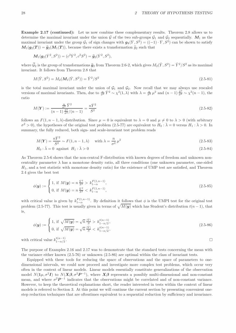
28 2 THEORY OF HYPOTHESIS TESTING
Example 2.17 (continued): Let us now combine these complementary results. Theorem 2.8 allows us todetermine the maximal invariant under the union G of the two sub-groups G1 and G2 sequentially. M1 as themaximal invariant under the group G1 of sign changes with g1(Y , S2) = ((−1) · Y , S2) can be shown to satisfyM1(g2(T )) = g2(M1(T )), because there exists a transformation g2 such that
M1(g2(Y 2, S2)) = (c2Y 2, c2S2) = g2(Y 2, S2),
where G2 is the group of transformations g2 from Theorem 2.6-2, which gives M2(Y , S2) = Y 2/S2 as its maximalinvariant. It follows from Theorem 2.8 that
M(Y , S2) = M2(M1(Y , S2)) = Y 2/S2 (2.5-81)
is the total maximal invariant under the union of G1 and G2. Now recall that we may always use rescaledversions of maximal invariants. Then, due to n
σ2 Y 2 ∼ χ2(1, λ) with λ = nσ2 µ2 and (n − 1) S2
σ2 ∼ χ2(n − 1), theratio
M(Y ) :=nσ2 Y 2
(n − 1) S2
σ2 /(n − 1)=
nY 2
S2(2.5-82)
follows an F (1, n − 1, λ)-distribution. Since µ = 0 is equivalent to λ = 0 and µ �= 0 to λ > 0 (with arbitraryσ2 > 0), the hypotheses of the original test problem (2.5-77) are equivalent to H0 : λ = 0 versus H1 : λ > 0. Insummary, the fully reduced, both sign- and scale-invariant test problem reads
M(Y ) =nY 2
S2∼ F (1, n − 1, λ) with λ =
n
σ2µ2 (2.5-83)
H0 : λ = 0 against H1 : λ > 0 (2.5-84)
As Theorem 2.5-6 shows that the non-central F-distribution with known degrees of freedom and unknown non-centrality parameter λ has a monotone density ratio, all three conditions (one unknown parameter, one-sidedH1, and a test statistic with monotone density ratio) for the existence of UMP test are satisfied, and Theorem2.4 gives the best test
φ(y) :=
⎧⎨⎩ 1, if M(y) = n Y 2
S2 > kF (1,n−1)1−α ,
0, if M(y) = n Y 2
S2 < kF (1,n−1)1−α ,
(2.5-85)
with critical value is given by kF (1,n−1)1−α . By definition it follows that φ is the UMPI test for the original test
problem (2.5-77). This test is usually given in terms of√
M(y) which has Student’s distribution t(n− 1), thatis,
φ(y) :=
⎧⎨⎩ 1, if√
M(y) =√
n |Y |S > k
t(n−1)1−α/2 ,
0, if√
M(y) =√
n |Y |S < k
t(n−1)1−α/2 ,
(2.5-86)
with critical value kt(n−1)1−α/2 . �
The purpose of Examples 2.16 and 2.17 was to demonstrate that the standard tests concerning the mean withthe variance either known (2.5-76) or unknown (2.5-86) are optimal within the class of invariant tests.
Equipped with these tools for reducing the space of observations and the space of parameters to one-dimensional intervals, we could now proceed and investigate more complex test problems, which occur veryoften in the context of linear models. Linear models essentially constitute generalizations of the observationmodel N(1µ, σ2I) to N(Xβ, σ2P−1), where Xβ represents a possibly multi-dimensional and non-constantmean, and where σ2P−1 indicates that the observations might be correlated and of non-constant variance.However, to keep the theoretical explanations short, the reader interested in tests within the context of linearmodels is referred to Section 3. At this point we will continue the current section by presenting convenient one-step reduction techniques that are oftentimes equivalent to a sequential reduction by sufficiency and invariance.

2.5 Best critical regions 29
2.5.6 Reduction to the Likelihood Ratio and Rao’s Score statistic
At the beginning of the current Section 2.5, where we discussed the case of testing against a simple H1, we haveseen that the density ratio f(y; θ1)/f(y; θ0), used as a test statistic for the MP test as defined in (2.5-26) by theNeyman-Pearson Lemma, may be simplified such that a single sufficient statistic can be used as an equivalenttest statistic. Whenever a test problem has a one-sided H1 (but still only one single unknown parameter), thenthat sufficient statistic must have a distribution with a monotone density ratio in order for a UMP test to exist.If multiple parameters are unknown, then our approach was to shrink the dimension of the parameter spaceto 1 in order to have a one-dimensional test statistic at one’s disposal. Such a test statistic was derived asthe maximal invariant under a group of transformations, which lead us to tests that are UMP among all testsinvariant under these transformations.
As a test problem may be invariant under numerous sub-groups of transformations (such as the one inExample 2.17), a manual step-wise reduction of a test problem by invariance can become quite cumbersome.Therefore, we will investigate ways for obtaining a UMPI test in a more direct manner. We will see that thereare in fact two equivalent methods for reducing a test problem about n observations (or equally well about m
minimal sufficient statistics) and m unknown parameters to a one-parameter problem with a one-sided H1.
Reduction to the Likelihood Ratio statistic. Let us consider the problem of testing H0 : θ ∈ Θ0 againstH1 : θ ∈ Θ1 on the basis of observations Y with true density function in
F = {f(y; θ) : θ ∈ Θ} .
Inspection of the density ratio f(y; θ1)/f(y; θ0), used for testing a simple H0 versus a simple H1 by the Neyman-Pearson Lemma, reveals that this quantity is not unique anymore if the hypotheses are composite, i.e. if θ0
and θ1 are elements of intervals Θ0 and Θ1. In that case it would not be clear at which values θ0 and θ1 thedensity ratio should be evaluated. This situation is of course not improved if the densities comprise multipleunknown parameters θ0 and θ1. One approach to removing the ambiguity of the density ratio consists in takingthe maximum value of the density function over Θ0 and over Θ1, that is, to determine the value of
maxθ∈Θ1 f(y; θ)maxθ∈Θ0 f(y; θ)
. (2.5-87)
Since the densities in (2.5-87) are now treated as functions of θ rather than of y, it is necessary to switch thearguments, or formally to introduce a new function from Θ to R, which is defined as
L(θ; y) := f(y; θ), (2.5-88)
and which treats y as given constants. L is called the likelihood function (for y), and the fraction
maxθ∈Θ0 L(θ; y)maxθ∈Θ1 L(θ; y)
(2.5-89)
denotes the generalized likelihood ratio. Notice that in this definition the nominator and denominatorhave been switched with respect to the generalized density ratio (2.5-87). To take this change into accountwhen comparing this ratio with the critical value, we only need to switch the </>-relation accordingly. If thehypotheses are such that Θ = Θ0 ∪ Θ1, then we may modify (2.5-89) slightly into
GLR :=maxθ∈Θ0 L(θ; y)maxθ∈Θ L(θ; y)
. (2.5-90)
The only difference between (2.5-90) and (2.5-89) is that (2.5-90) may take the value 1, because Θ0 is a subsetof Θ (see also Koch, 1999, p. 279, for a discussion of the properties of the generalized likelihood ratio).
All the examples discussed so far and all the applications to be investigated in Sections 3 and 4 allow us torewrite the hypotheses H0 : θ ∈ Θ0 and H1 : θ ∈ Θ1 in the form of linear constraints (restrictions)
H0 : Hθ = w versus H1 : Hθ
⎧⎪⎪⎪⎨⎪⎪⎪⎩<
>
�=
⎫⎪⎪⎪⎬⎪⎪⎪⎭w, (2.5-91)
where H is an (r × u)-matrix with known constants and rank r, and where w is an (r × 1)-vector of knownconstants.

30 2 THEORY OF HYPOTHESIS TESTING
Example 2.18: In the Examples 2.13, 2.14, and 2.16 we considered the problems of testing the specificationH0 : µ = µ0 of the mean parameter against the alternative specifications H1 : µ < µ0, H1 : µ > µ0, andH1 : µ �= µ0 on the basis of normally distributed observations with known variance. These hypotheses may berewritten in the form (2.5-91) by using the vectors/matrices θ := [ µ ], H := [ 1 ], and w := [ µ0 ], which are allscalars in this case.
In Example 2.17, we investigated the problem of testing H0 : µ = µ0 versus H1 : µ �= µ0 in the same class ofnormal distributions, but with unknown variance. These hypotheses are expressed as in (2.5-91) by defining
θ :=
⎡⎣ µ
σ2
⎤⎦ , H := [ 1, 0 ], and w := [ µ0 ]. �
When the hypotheses are given in terms of linear restrictions (2.5-91), then the maxima in (2.5-90) may beinterpreted in the following way. The value θ for which the likelihood function in the nominator of (2.5-90)attains its maximum over Θ0, or equivalently for which the constraint Hθ = w holds, is called the restrictedmaximum likelihood (ML) estimate for θ. On the other hand, the value θ for which the likelihoodfunction in the denominator of (2.5-90) attains its maximum over the entire parameter space Θ, denotes thenthe unrestricted maximum likelihood (ML) estimate for θ.
If we assume that the likelihood function is at least twice differentiable with positive definite Hessian, thenthe restricted ML estimate θ is obtained as the solution of
∂
∂θ(L(θ; y)− k′(Hθ − w)) = 0, (2.5-92)
where k denotes an (r × 1)-vector of unknown Lagrange multipliers. The unrestricted ML estimate θ followsas the solution of the likelihood equation
∂
∂θL(θ; y) = 0. (2.5-93)
Then, rewriting (2.5-90) in terms of the ML estimators and the random vector Y yields
GLR(Y ) =L(θ; Y )
L(θ; Y ). (2.5-94)
This is the reciprocal of the statistic that Koch (1999, Chap. 4.2) and Teunissen (2000, Chap. 3) use to derivethe test of the general hypothesis in the normal Gauss-Markov model. In that case, which will also be addressedin detail in Section 3 of this thesis, the restricted und unrestricted ML estimates are equivalent to the restrictedand unrestricted least squares estimates. However, it shall already be mentioned here that there are importantcases where the Gauss-Markov model is not restricted to the class of normal distributions, but where thelikelihood function may depend on additional distribution parameters (see Application 7). For this reason, wewill maintain the more general notation in terms of the likelihood function and the restricted/unrestricted MLestimates, and we will speak of restricted/unrestricted least squares estimates only if we apply a class of normaldistributions.
In certain cases, it will sometimes be more convenient to use a logarithmic version of the GLR, that is,
−2 lnGLR = −2 lnL(θ; Y )
L(θ; Y )= −2
(ln L(θ; Y ) − ln L(θ; Y )
). (2.5-95)
Due to the strictly increasing monotonicity of the logarithmus naturalis, the estimates θ and θ remain unchangedif, as in (2.5-95), the so-called log-likelihood function
L(θ; y) := lnL(θ; y) (2.5-96)
is maximized instead of the likelihood function (2.5-88). This property guarantees that the restricted MLestimate θ is also the solution of
∂
∂θ(L(θ; y) − k′(Hθ − w)) = 0, (2.5-97)
and that the unrestricted ML estimate θ is the solution of the log-likelihood equation
∂
∂θL(θ; y) = 0. (2.5-98)

2.5 Best critical regions 31
One advantage of this approach is that the logarithm of a Gaussian density will cancel out with the exponentialoperator, which results in a function that is easier to handle (see Example 2.19). We call the statistic TLR,defined by
TLR(Y ) := −2 lnGLR = −2(L(θ; Y ) − L(θ; Y )
), (2.5-99)
the likelihood ratio (LR) statistic.A test which uses (2.5-94) as test statistic is called the generalized likelihood ratio (GLR) test, given
by
φGLR(y) =
⎧⎨⎩ 1 if L(θ; y)/L(θ; y) < k∗α,
0 if L(θ; y)/L(θ; y) > k∗α,
(2.5-100)
where the critical value k∗α is such that φ has level α. Alternatively, the test
φLR(y) =
⎧⎨⎩ 1 if −2(L(θ; y) − L(θ; y)
)> kα,
0 if −2(L(θ; y) − L(θ; y)
)< kα,
(2.5-101)
based on the statistic (2.5-99) is called the likelihood ratio (LR) test. Both tests are truly equivalent becauseboth the corresponding statistics and critical values are strictly monotonic functions of each other.
It is easily verified that the test (2.5-100) is equivalent to the MP test (2.5-26) of Neyman and Pearson ifboth H0 and H1 are simple hypotheses and if θ is a single parameter, because the maxima then equal the pointvalues of the densities at Θ0 = {θ0} and Θ1 = {θ1}, respectively. Furthermore, if H1 is a one-sided hypothesis(with θ still being a single parameter) and if Y has a density with monotone density ratio, then the GLR/LRtest is also equal to the UMP test in Theorem 2.4 (see Lemma 2 in Birkes, 1990). Even more importantly, ifa test problem involves multiple parameters in a normal Gauss-Markov model, then the GLR/LR test is alsoidentical to the UMPI test obtained from a step-wise reduction by invariance. We will demonstrate this fact,which has been proven by Lehmann (1959b), in the following simple example and in greater detail in Section 3.
Example 2.19 (Example 2.17 revisited): The LR test of the normal mean with unknown variance.Let Y1, . . . , Yn be independently and normally distributed observations with common unknown mean µ andcommon unknown variance σ2. What is the LR test for testing H0 : µ = µ0 (σ2 > 0) versus H1 : µ �= µ0
(σ2 > 0) at level α?Using the fact that the joint density of independently distributed observations is the product of the univariate
densities, we obtain for the log-likelihood function
L(θ; y) := ln f(y; µ, σ2)
= lnn∏
i=1
1√2πσ
exp
{−1
2
(yi − µ
σ
)2}
=n∑
i=1
ln
[(2πσ2)−1/2 exp
{−1
2
(yi − µ
σ
)2}]
=n∑
i=1
[0 − 1
2ln(2π) − 1
2ln σ2 − 1
2σ2(yi − µ)2
]
= −n
2ln(2π) − n
2ln σ2 − 1
2σ2
n∑i=1
(yi − µ)2
Let us first determine the unrestricted ML estimates for µ and σ2 by applying (2.5-98). From the first orderconditions
∂
∂µL(θ; y) =
1σ2
n∑i=1
(yi − µ) = 0, (2.5-102)
∂
∂σ2L(θ; y) = − n
2σ2+
12σ4
n∑i=1
(yi − µ)2 = 0, (2.5-103)

32 2 THEORY OF HYPOTHESIS TESTING
we obtain the solutions
µ =1n
n∑i=1
yi (2.5-104)
and
σ2 =1n
n∑i=1
(yi − µ)2. (2.5-105)
Notice that σ2 differs from the sample variance S2 = 1n−1
∑ni=1(yi − µ)2. The restricted estimates result from
solving (2.5-97), that is,
∂
∂µ(L(θ; y) − k(µ − µ0)) =
1σ2
n∑i=1
(yi − µ) − k = 0,
∂
∂σ2(L(θ; y) − k(µ − µ0)) = − n
2σ2+
n
2σ4
n∑i=1
(yi − µ)2 = 0,
∂
∂k(L(θ; y) − k(µ − µ0)) = −(µ − µ0) = 0.
The third equation reproduces the restriction, that is
µ = µ0. (2.5-106)
Using this result, the second equation gives
σ2 =1n
n∑i=1
(yi − µ0)2. (2.5-107)
Substituting µ = µ0 and σ2 into the first equation results in the estimate
k =1σ2
n∑i=1
(yi − µ0) (2.5-108)
for the Lagrange multiplier. To evaluate the test statistics based on the generalized likelihood ratio, we need tocompute the likelihood function both at the unrestricted and the restricted estimates, which leads to
L(µ, σ2; y) = (2πσ2)−n/2 exp
{− 1
2σ2
n∑i=1
(yi − µ)2}
= (2π)−n/2(σ2)−n/2 exp{−n
2
}and
L(µ, σ2; y) = (2πσ2)−n/2 exp
{− 1
2σ2
n∑i=1
(yi − µ0)2}
= (2π)−n/2(σ2)−n/2 exp{−n
2
}.
With this, the GLR in (2.5-94) tales the value
GLR(y) =L(µ, σ2; y)L(µ, σ2; y)
=(
σ2
σ2
)−n/2
,
and the value of the LR statistic in (2.5-99) becomes
TLR(y) = −2 lnGLR = n lnσ2
σ2.
We will now show that TLR(Y ) (thus also the GLR statistic) is equivalent to the statistic M(Y ) in (2.5-83) ofthe UMPI test (2.5-85) for testing H0 : µ = µ0 = 0 (σ2 > 0) versus H1 : µ �= µ0 = 0 (σ2 > 0) at level α. Recallthat M(Y ) = n Y 2
S2 with sample mean Y = 1n
∑ni=1 Yi and sample variance S2 = 1
n−1
∑ni=1(Yi − Y )2. Then,
due to Y = µ and (n − 1)S2 = nσ2, we have
1 +M(Y )n − 1
= 1 +nY 2
(n − 1)S2= 1 +
µ2
σ2=
σ2 + µ2
σ2=
1n
∑ni=1(yi − µ)2 + µ2
σ2=
1n
∑ni=1 y2
i
σ2=
σ2
σ2.

2.5 Best critical regions 33
Thus, TLR(Y ) = n ln(1 + M(Y )n−1 ) is a strictly monotonically increasing function of M(Y ). If we transform the
critical value C = kF (1,n−1)1−α of the UMPI test (2.5-85) accordingly into C∗ = n ln(1 + C
n−1 ), then the LR test
φLR(y) :=
⎧⎨⎩ 1, if TLR(y) = n ln �σ2
�σ2 > C∗,
0, if TLR(y) = n ln �σ2
�σ2 < C∗,(2.5-109)
will produce the same result as the UMPI test (2.5-85). �
Reduction to Rao’s Score statistic. Another way to formulate the Likelihood Ratio statistic (2.5-99)results from applying a two-term Taylor series to the log-likelihood function (2.5-96). For this purpose, wewill assume throughout this thesis that the first two derivatives of the log-likelihood function exist. If theunrestricted ML estimate is used as Taylor point, then we obtain
L(θ; y) = L(θ; y) +∂L(θ; y)
∂θ
∣∣∣∣�θ
+12(θ − θ)′
∂2L(θ; y)∂θ∂θ′
∣∣∣∣θ∗
(θ − θ). (2.5-110)
The vector of first partial derivatives
S(θ; y) :=∂L(θ; y)
∂θ(2.5-111)
is called the (log-likelihood or efficient) score. The Hessian matrix of second partial derivatives will bedenoted by
H(θ; y) :=∂2L(θ; y)
∂θ∂θ′ . (2.5-112)
This matrix, which appears in the exact residual term of the Taylor series (2.5-110), is evaluated at possiblydifferent points between θ and θ. Now, it follows from the log-likelihood equations (2.5-98) that the score vectorvanishes at θ, that is S(θ; y) = 0. Then, evaluation of (2.5-110) at the restricted ML estimate θ yields
L(θ; y) = L(θ; y) +12(θ − θ)′H(θ∗; y)(θ − θ),
or
−2(L(θ; y) − L(θ; y)
)= −(θ − θ)′H(θ∗; y)(θ − θ).
We will now use an argument by Stuart et al. (1999, p. 57) stating that, in terms of random variables, H(θ∗; Y ) ≈E{H(θ; Y )} for large n. Note that if the log-likelihood function is naturally given as a quadratic function ofθ, then the Hessian will be a matrix of constants. In that case, we will write the Hessian as HY , which is thenidentical to E{HY }. The expectation of the negative Hessian of the log-likelihood function, that is
I(θ; Y ) := E{−H(θ; Y )} (2.5-113)
is called the information matrix. With this, we obtain for the test statistic
TLR(Y ) = −2(L(θ; Y ) − L(θ; Y )
)≈ (θ − θ)′E{−H(θ; Y )(θ − θ)
= (θ − θ)′I(θ; Y )(θ − θ) (2.5-114)
In a second step we apply a one-term Taylor series to the score with Taylor point θ, that is
S(θ; y) = S(θ; y) +∂S(θ; y)
∂θ
∣∣∣∣θ∗∗
(θ − θ).
Then we evaluate the score at the maximum likelihood estimate θ, which gives
S(θ; y) = 0 = S(θ; y) + H(θ∗∗; y)(θ − θ).

34 2 THEORY OF HYPOTHESIS TESTING
Now, the same argument applies as above, i.e. H(θ∗∗; Y ) ≈ E{H(θ; Y )} for large n, which gives
I(θ; Y )(θ − θ) ≈ S(θ; Y ),
or
θ − θ ≈ I−1(θ; Y )S(θ; Y )
Again, if the log-likelihood function is quadratic in θ, then the above approximations become exact.Substituting the last equation for θ − θ into (2.5-114) finally yields
TLR(Y ) ≈ S′(θ; Y )I−1(θ; Y )S(θ; Y ) =: TRS(Y ). (2.5-115)
The statistic TRS(Y ) is called (the) Rao’s Score (RS) statistic (see Equation 6e.3.6 in Rao, 1973, p. 418),which was originally proposed in Rao (1948) for the problem of testing H0 : θ = θ0 versus H1 : θ > θ0 with asingle unknown parameter θ. In this one-dimensional case, Rao’s Score statistic takes the simple form
TRS(Y ) = S2(θ0; Y )/I(θ0; Y ). (2.5-116)
Example 2.20 (Example 2.17 revisited): The RS test of the normal mean with unknown variance.Let Y1, . . . , Yn be independently and normally distributed observations with common unknown mean µ andcommon unknown variance σ2. What is the RS test for testing H0 : µ = µ0 (σ2 > 0) versus H1 : µ �= µ0
(σ2 > 0) at level α?To determine the value of Rao’s Score statistic (2.5-115), we need to determine the log-likelihood score and
the inverse of the information matrix, and then evaluate these quantities at the restricted ML estimates. Thefirst partial derivatives of the log-likelihood function with respect to µ and σ2 have already been determined as(2.5-102) and (2.5-103) in Example 2.19. Thus, the log-likelihood score vector follows to be
S(θ; y) =
⎡⎣ ∂L(µ,σ2;y)∂µ
∂L(µ,σ2;y)∂σ2
⎤⎦ =
⎡⎢⎢⎣1
σ2
n∑i=1
(yi − µ)
− n2σ2 + 1
2σ4
n∑i=1
(yi − µ)2
⎤⎥⎥⎦ .
The Hessian of the log-likelihood function comprises the second partial derivatives with respect to all unknownparameters. For the current example, these are
∂2L(µ, σ2; y)∂µ∂µ
= − n
σ2,
∂2L(µ, σ2; y)∂µ∂σ2
= − 1σ4
n∑i=1
(yi − µ),
∂2L(µ, σ2; y)∂σ2∂µ
= − 1σ4
n∑i=1
(yi − µ),
∂2L(µ, σ2; y)∂σ2∂σ2
=n
2σ4− 1
σ6
n∑i=1
(yi − µ)2.
Then, the information matrix follows to be
I(θ; Y ) = E{−H(θ; Y )}
= E
⎧⎪⎪⎨⎪⎪⎩−
⎡⎢⎢⎣ − nσ2 − 1
σ4
n∑i=1
(Yi − µ)
− 1σ4
n∑i=1
(Yi − µ)2 n2σ4 − 1
σ6
n∑i=1
(Yi − µ)2
⎤⎥⎥⎦⎫⎪⎪⎬⎪⎪⎭
=
⎡⎢⎢⎣nσ2
1σ4
n∑i=1
(E{Yi} − µ)
1σ4
n∑i=1
(E{Yi} − µ) − n2σ4 + 1
σ6
n∑i=1
E{(Yi − µ)2}
⎤⎥⎥⎦ .

2.5 Best critical regions 35
Due to the definitions E{Yi} = µ and E{(Yi − µ)2} = σ2 of the first moment and the second central moment,respectively, the off-diagonal components of the information matrix vanish, and we obtain
I(θ; Y ) =
⎡⎣ nσ2 0
0 n2σ4
⎤⎦ .
Then, using the fact that the restricted ML estimate for µ is µ = µ0, Rao’s Score statistic in (2.5-115) becomes
TRS(Y ) = S ′(µ, σ2; Y )I−1(µ, σ2; Y )S(µ, σ2; Y )
=
⎡⎢⎢⎣1�σ2
n∑i=1
(Yi − µ0)
− n2�σ2 + 1
2σ4
n∑i=1
(Yi − µ0)2
⎤⎥⎥⎦′ ⎡⎣ n
�σ2 0
0 n2�σ2
⎤⎦−1⎡⎢⎢⎣
1�σ2
n∑i=1
(Yi − µ0)
− n2�σ2 + 1
2σ4
n∑i=1
(Yi − µ0)2
⎤⎥⎥⎦
=
⎡⎢⎣ 1�σ2
n∑i=1
(Yi − µ0)
0
⎤⎥⎦′ ⎡⎣ �σ2
n 0
0 2�σ2
n
⎤⎦⎡⎢⎣ 1
�σ2
n∑i=1
(Yi − µ0)
0
⎤⎥⎦=
1nσ2
(n∑
i=1
(Yi − µ0)
)2
.
Two aspects are typical for Rao’s Score statistic. Firstly, the log-likelihood score vanishes in the direction ofσ2. This happens necessarily because σ2 is not restricted by H0. Therefore, the unrestricted ML estimateof such a free parameter will certainly maximize the log-likelihood function in that direction. Secondly, theinformation matrix is diagonal, reflecting the fact that both parameters are determined independently. Thesetwo properties, which are true also for more complex testing problems such as for the applications in Sections3 and 4, simplify the determination of Rao’s Score statistic considerably.
If we recall from (2.5-108) in Example 2.19 that 1�σ2
∑ni=1(Yi−µ0) is the estimator for the Lagrange multiplier,
we may rewrite Rao’s Score statistic in the form
TRS(Y ) =σ2
n
(1σ2
n∑i=1
(Yi − µ0)
)2
=σ2
nk2.
For this reason, Rao’s Score statistic is often called the Lagrange Multiplier (LM) statistic, a term whichwas probably first used by Silvey (1959) and which is used typically in the field of econometrics.
Let us assume that the observations have been centered such that the hypotheses are about µ0 = 0, asdemonstrated in Example 2.16. As for the relation between TLR and the UMPI test statistic derived in Example2.19, we can show that TRS is not identical with the UMPI test statistic, but a strictly monotonic functionthereof. Recall from Example 2.19 that M(Y )/(n − 1) = µ2/σ2 and 1 + M(Y )/(n − 1) = (σ2 + µ2)/σ2. Withthis, we obtain
n1
n−1M(Y )
1 + 1n−1M(Y )
= nµ2
σ2/σ2
σ2= n
µ2
σ2=
1nσ2
(n∑
i=1
Yi
)2
= TRS .
Therefore, Rao’s Score test
φRS(y) :=
⎧⎨⎩ 1, if TRS(y) = �σ2
n k2 > C∗,
0, if TRS(y) = �σ2
n k2 < C∗,(2.5-117)
with critical value C∗ = n C/n−11+C/(n−1) will be exactly the same as the UMPI test (2.5-85) with critical value
C = kF (1,n−1)1−α . �

36 3 THEORY AND APPLICATIONS OF MISSPECIFICATION TESTS IN THE NORMAL GMM
3 Theory and Applications of Misspecification Tests in the Normal
Gauss-Markov Model
3.1 Introduction
In this section we will consider a number of very common test problems within the context the normal Gauss-Markov model (GMM)
Y = Xβ + E, (3.1-118)
Σ = Σ{E} = σ2P−1 (3.1-119)
with normally distributed zero-mean errors E, known design matrix X ∈ Rn×m of full rank, known positive
definite weight matrix P ∈ Rn×n, and parameters β ∈ R
m×1 and σ2 ∈ R+, respectively. Thus, we may write
the resulting class of distributions with respect to the observables Y as
W = {N (Xβ, σ2P−1)
: β ∈ Rm×1, σ2 ∈ R
+}, (3.1-120)
which corresponds to the space Θ = Rm×1 × R
+ of parameters θ = (β, σ2) and to the class of multivariatenormal density functions
F = {f (y; β, σ2)
: β ∈ Rm×1, σ2 ∈ R
+},
of multivariate normal density functions, defined by
f(y; β, σ2) = (2π)−n/2(det σ2P−1)−1/2 exp{− 1
2σ2(y − Xβ)′P (y − Xβ)
}(3.1-121)
(see Equation 2.125 in Koch, 1999, p. 117). We will further assume that the unknown true parameter vector θ
is one element of Θ.Frequently, the numerical value σ2
0 for σ2 is known a priori. In this case we will rewrite the class ofdistributions as
W = {N (Xβ, σ20P
−1)
: β ∈ Rm×1}, (3.1-122)
the space of parameters θ = β as Θ = Rm×1, and the corresponding class of density functions as
F = {f (y; β) : β ∈ Rm×1} (3.1-123)
with
f(y; β) = (2π)−n/2(detσ20P−1)−1/2 exp
{− 1
2σ20
(y − Xβ)′P (y − Xβ)}
Notice that, by setting X := 1 and P := I, we obtain the observation model used in Examples 2.16 and 2.17(depending on whether σ2 is known or unknown a priori).
As the parameter space comprises two types of parameters, we will naturally consider two categories of testproblems. The first one is about testing the parameters β appearing in the functional model (3.1-118), and thesecond one is about testing the variance factor σ2, which is part of the stochastic model. Solutions to these testproblems are well known (see, for instance, Koch, 1999; Teunissen, 2000) and belong to the standard proceduresof geodetic adjustment theory. Therefore, rather than to repeat common knowledge, the purpose of this sectionis to reconceptualize these tests, in particular the test statistics, by deriving them as optimal procedures. Forthis purpose, we will exploit symmetry assumptions, that is, invariance principles with respect to the powerfunction in the same way as demonstrated in Section 2 for some simpler test problems. It will turn out thatthe standard outlier tests, significance tests, tests of linear hypotheses, and the test of the variance factor owemuch of their uselfulness to the fact that they may all be derived as uniformly most powerful invariant tests.

3.2 Derivation of optimal tests concerning parameters of the functional model 37
3.2 Derivation of optimal tests concerning parameters of the functional model
So far we have confined ourselves to problems, where the hypothesis that parameters take particular values wasto be tested against some simple or composite alternative. However, limitation to such problems is unnecessarilyrestrictive. There are situations where we would rather want to test whether a set of linear functions of theparameters takes particular values. As a common example, it is desired in deformation analysis to test whetherdifferences of coordinates are zero, or whether they differ significantly (see Application 3). We have already seenin (2.5-91) of Section 2.5.6 that hypotheses may take the form of linear constraints (restrictions) concerning theparameters to be tested. This model also fits conveniently into the framework of the normal GMM (3.1-118 +3.1-119). In the current section, we shall restrict attention to hypotheses concerning parameters β within thefunctional model (3.1-118), which may then be written as constraints
H0 : Hβ = w versus H1 : Hβ �= w, (3.2-124)
where H ∈ Rm2×m (with m2 ≤ m) denotes a matrix of full rank.
This general model setup may be simplified in various ways before addressing the fundamental questionof optimality procedures. The first step will be to reparameterize the GMM and the constraints such thatthe hypotheses become direct propositions about the values of the unknown parameters rather than about thevalues of functions thereof. Furthermore, to exploit symmetries within the parameter space effectively, it willalso be convenient to center these transformed hypotheses about zero. Finally, we shall simplify the stochasticmodel (3.1-119) by transforming the observations into uncorrelated variables with constant variance.
After carrying out these preprocessing steps, we will reduce the testing problem by sufficiency and invariancein a similar manner to the approach presented in Section 2. Then, after reversing the preprocessing steps, wewill obtain, as the main result of this section, the UMPI test for testing the hypotheses in (3.2-124).
The individual steps of this preprocessing and reduction procedure will now be carried out within thefollowing subsections:
1. Reparameterization of the test problem.
2. Centering of the hypotheses.
3. Full decorrelation/homogenization of the observations.
4. Reduction to independent sufficient statistics with elimination of additional functional parameters.
5. Reduction to a maximal invariant statistic.
6. Back-substitution (reversal of steps 1.-4).
3.2.1 Reparameterization of the test problem
Following Meissl (1982, Section C.2.2), we expand the m2 × m-matrix H by some (m − m2) × m-matrix M
into an invertible m×m block matrix and introduce new parameters β(r)1 ∈ R
m1×1 (where m1 := m−m2) andβ
(r)2 ∈ R
m2×1 with⎡⎣ β(r)1
β(r)2
⎤⎦ :=
⎡⎣ M
H
⎤⎦β. (3.2-125)
Using the invertibility assumption we obtain the equivalent relation
β =
⎡⎣ M
H
⎤⎦−1 ⎡⎣ β(r)1
β(r)2
⎤⎦ .
Then, multiplying this equation with X from the left yields
Xβ = X
⎡⎣ M
H
⎤⎦−1 ⎡⎣ β(r)1
β(r)2
⎤⎦ =:[X
(r)1 X
(r)2
]⎡⎣ β(r)1
β(r)2
⎤⎦ . (3.2-126)

38 3 THEORY AND APPLICATIONS OF MISSPECIFICATION TESTS IN THE NORMAL GMM
Notice that this definition allows us to derive the following expression for the original design matrix X fromthe implication
X
⎡⎣ M
H
⎤⎦−1
=:[X
(r)1 X
(r)2
]⇒ X =
[X
(r)1 X
(r)2
]⎡⎣ M
H
⎤⎦ . (3.2-127)
Using (3.2-126) we may substitute the original functional model (3.1-118) by
Xβ = X(r)1 β
(r)1 + X
(r)2 β
(r)2 (3.2-128)
and, in light of (3.2-125), the linear restriction (3.2-124) by
Hβ = β(r)2 . (3.2-129)
This reparameterization leads to an equivalent testing problem which involves the transformed version X(r) =[ X(r)
1 X(r)2 ] of the original design matrix X = [ X1 X2 ] in partitioned form. We will describe this simplified
class of test problems by the new observation model
Y ∼ N(X
(r)1 β
(r)1 + X
(r)2 β
(r)2 , σ2P−1
)(3.2-130)
(where the true value of σ2 may be known or unknown a priori), and by the new hypotheses
H0 : β(r)2 = w versus H1 : β
(r)2 �= w. (3.2-131)
3.2.2 Centering of the hypotheses
Similarly to the data transformation in Example 2.16 we may subtract the generalized constant mean X(r)2 w
from the data, that is,
Y (c) := Y − X(r)2 w. (3.2-132)
While this transformation leaves the covariance matrix as the second central moment unchanged, it changes theexpectation to
E{Y − X
(r)2 w
}= E
{X
(r)1 β
(r)1 + X
(r)2 β
(r)2 − X
(r)2 w
}= E
{X
(r)1 β
(r)1 + X
(r)2
(β
(r)2 − w
)}. (3.2-133)
Setting β(rc)2 := β
(r)2 − w leads to the new observation model
Y (c) ∼ N(X
(r)1 β
(r)1 + X
(r)2 β
(rc)2 , σ2P−1
), (3.2-134)
where the true value of σ2 may be known or unknown a priori. The hypotheses in terms of ersatz parametersβ
(rc)2 are then evidently given by
H0 : β(rc)2 = 0 versus H1 : β
(rc)2 �= 0. (3.2-135)
3.2.3 Full decorrelation/homogenization of the observations
A Cholesky decomposition of the weight matrix into
P = GG′, (3.2-136)
where G stands for an invertible lower triangular matrix, allows for a full decorrelation or homogenization ofthe observations by virtue of the one-to-one transformation
Y (ch) := G′Y (c) (3.2-137)
(cf. Koch, 1999, p. 154). The expectation of the transformed observables becomes
E{G′Y (c)
}= G′
(X
(r)1 β
(r)1 + X
(r)2 β
(rc)2
)= G′X(r)
1 β(r)1 + G′X(r)
2 β(rc)2 .

3.2 Derivation of optimal tests concerning parameters of the functional model 39
The fact that Y (ch) has covariance matrix σ2I follows directly from an application of error propagation to thelinear function G′Y (c), which yields with (3.2-136)
Σ{G′Y (c)
}= G′Σ
{Y (c)
}G = G′σ2P−1G = σ2G′ (GG′)−1
G
= σ2G′(G′)−1G−1G = σ2I.
After introducing the transformed block design matrices X(rh)1 := G′X(r)
1 and X(rh)2 := G′X(r)
2 , the trans-formed observation model then reads
Y (ch) ∼ N(X
(rh)1 β
(r)1 + X
(rh)2 β
(rc)2 , σ2I
), (3.2-138)
where the true value of σ2 may be known or unknown a priori. As homogenization does not transform param-eters, the hypotheses may still be written as in (3.2-135), that is,
H0 : β(rc)2 = 0 versus H1 : β
(rc)2 �= 0. (3.2-139)
Whenever a test problem with structure (3.1-120/3.1-122, 3.2-124) or (3.2-130, 3.2-131) or (3.2-134, 3.2-135)is given, it may be transformed directly into (3.2-138, 3.2-139), which will turn out to be the most suitablestructure for subsequent reductions by sufficiency and invariance.
3.2.4 Reduction to minimal sufficient statistics with elimination of nuisance parameters
To reduce the observations Y (ch) by sufficiency, we need to generalize the result of Examples 2.10 and 2.11 tothe case of the linear model.
Proposition 3.1. In the normal Gauss-Markov model Y ∼ N(Xβ, σ2I), the least squares estimators
X ′Xβ = X ′Y (3.2-140)
and
(n − m)σ2 = (Y − Xβ)′(Y − Xβ) (3.2-141)
constitute independently distributed and minimally sufficient statistics for β and σ2, respectively.
Proof. Using the estimates defined by (3.2-140) and (3.2-141), the multivariate normal density (3.1-121) maybe rewritten as
f(y; β, σ2) = (2π)−n/2(detσ2I)−1/2 exp{− 1
2σ2(y − Xβ)′(y − Xβ)
}= (2πσ2)−n/2 exp
{− 1
2σ2
((n − m)σ2 + (β − β)′X ′X(β − β)
)}IRn(y).
Thus, it follows from Neyman’s Factorization Theorem 2.2 that β and (n−m)σ2 are jointly sufficient statisticsfor β and σ2. Then, Arnold (1981, p. 65) shows that these statistics are complete, which implies minimality(see Arnold, 1990, p. 346), and independently distributed with
β ∼ N(β, σ2(X ′X)−1) (3.2-142)
and
(n − m)σ2/σ2 ∼ χ2(n − m). (3.2-143)
Next, we will rewrite this fundamental result in terms of partitioned parameters as demanded by the obser-vation model (3.2-138).

40 3 THEORY AND APPLICATIONS OF MISSPECIFICATION TESTS IN THE NORMAL GMM
Proposition 3.2. In the normal linear Gauss-Markov model Y ∼ N(X1β1 + X2β2, σ2I) with partitioned
parameters β1 ∈ Rm1×1 and β2 ∈ R
m2×1, the least squares estimators⎡⎣ X ′1X1 X ′
1X2
X ′2X1 X ′
2X2
⎤⎦⎡⎣ β1
β2
⎤⎦ =
⎡⎣ X ′1Y
X ′2Y
⎤⎦ , short :
⎡⎣ N11 N12
N21 N22
⎤⎦⎡⎣ β1
β2
⎤⎦ =
⎡⎣ n1
n2
⎤⎦ (3.2-144)
and
(n − m1 − m2)σ2 = (Y − X1β1 − X2β2)′(Y − X1β1 − X2β2) (3.2-145)
constitute minimally sufficient statistics for β1, β2, and σ2, respectively. Furthermore, the statistics [β′1 β′
2]and σ2 are independently distributed with⎡⎣ β1
β2
⎤⎦ ∼ N
⎛⎜⎝⎡⎣ β1
β2
⎤⎦ , σ2
⎡⎣ X ′1X1 X ′
1X2
X ′2X1 X ′
2X2
⎤⎦−1⎞⎟⎠ (3.2-146)
and
(n − m1 − m2)σ2/σ2 ∼ χ2(n − m1 − m2). (3.2-147)
Before considering a reduction of Y (ch) to sufficient statistics we may notice that the observation model(3.2-138) comprises functional parameters β
(r)1 not subject to hypotheses. Therefore, we may eliminate them
from the normal equations (3.2-144) (cf. Schuh, 2006a, Section 1.2.1) without changing the test problemitself. First we rewrite the partitioned normal equations (3.2-144) in terms of reparameterized, centered, andhomogenized quantities, that is,
X′(rh)1 X
(rh)1 β
(r)1 + X
′(rh)1 X
(rh)2 β
(rc)2 = X
′(rh)1 Y (ch) (3.2-148)
X′(rh)2 X
(rh)1 β
(r)1 + X
′(rh)2 X
(rh)2 β
(rc)2 = X
′(rh)2 Y (ch) (3.2-149)
Isolation of β(r)1 in (3.2-148) yields
β(r)1 =
(X
′(rh)1 X
(rh)1
)−1 (X
′(rh)1 Y (ch) − X
′(rh)1 X
(rh)2 β
(rc)2
), (3.2-150)
and after substitution into (3.2-149)
β(rc)2 = N
(−1)22
(X
′(rh)2 − X
′(rh)2 X
(rh)1
(X
′(rh)1 X
(rh)1
)−1
X′(rh)1
)Y (ch) (3.2-151)
with Schur complement
N(−1)22 :=
(X
′(rh)2 X
(rh)2 − X
′(rh)2 X
(rh)1
(X
′(rh)1 X
(rh)1
)−1
X′(rh)1 X
(rh)2
)−1
(3.2-152)
as abbreviation. We will not give N(−1)22 the index .(rh) because (1) this matrix naturally refers to the model
with two groups of parameters β(r)1 and β
(r)1 , and (2) it may be written directly in terms of non-homogeneous
quantities, that is,
N(−1)22 =
(X
′(r)2 PX
(r)2 − X
′(r)2 PX
(r)1
(X
′(r)1 PX
(r)1
)−1
X′(r)1 PX
(r)2
)−1
.
The residuals in the observation model (3.2-138) are defined as
E(rch) = Y (ch) − X(rh)1 β
(r)1 − X
(rh)2 β
(rc)2 , (3.2-153)
and may, after substitution of (3.2-150), be written as
E(rch) =(
I − X(rh)1
(X
′(rh)1 X
(rh)1
)−1
X′(rh)1
)(Y (ch) − X
(rh)2 β
(rc)2
). (3.2-154)

3.2 Derivation of optimal tests concerning parameters of the functional model 41
If the true value of the variance of unit weight must be estimated, then these two alternative formulations forthe residuals correspond to the following expressions for the estimator of σ2:
(n − m1 − m2)σ2(rch) = E′(rch)E(rch)
=(Y (ch) − X
(rh)1 β
(r)1 − X
(rh)2 β
(rc)2
)′ (Y (ch) − X
(rh)1 β
(r)1 − X
(rh)2 β
(rc)2
)=
(Y (ch) − X
(rh)2 β
(rc)2
)′(I − X
(rh)1
(X
′(rh)1 X
(rh)1
)−1
X′(rh)1
)(Y (ch) − X
(rh)2 β
(rc)2
).
Instead of using the vector β(rc)2 with possibly fully populated weight matrix, it will be much more convenient
to operate with the fully decorrelated and homogenized vector
β(rch)2 := G′
22β(rc)2 (3.2-155)
which is also sufficient for β(rc)2 as a one-to-one function of β
(rc)2 . Here, G22 represents the (invertible) lower
triangular matrix obtained from the Cholesky factorization P22 :=(N
(−1)22
)−1
= G22G′22. After reducing the
observation model (3.2-138) by sufficiency, we now have a test problem about ersatz observations [ β′(rch)2 , σ2 ]
with reduced dimension (m2 + 1). The hypotheses
H0 : β(rch)2 = 0 versus H1 : β
(rch)2 �= 0 (3.2-156)
follow from (3.2-156) by observing that β(rch)2 = 0 if and only if β
(rc)2 = 0 and β
(rch)2 �= 0 if and only if β
(rc)2 �= 0.
3.2.5 Reduction to a maximal invariant statistic
In this step we seek to reduce the test problem in terms of independent sufficient statistics by invariance in thesame way as we did in Example 2.17. The only difference will be that in the present case we cannot apply signinvariance as the expectation is now given by a non-constant mean vector. Instead we will verify that the testproblem is invariant under the group of orthogonal transformations acting on the mean vector β
(rch)2 .
Case 1: σ2 = σ20 known. Let us begin with the simpler case that the true value of the variance factor is
known a priori. First we note that each orthogonal transformation
g1(β(rch)2 ) = Γβ
(rch)2
in G1 results in a change of distribution from β(rch)2 ∼ N(β(rch)
2 , σ20I) to Γβ
(rch)2 ∼ N(Γβ
(rch)2 , σ2
0I), where thecovariance matrix of Γβ
(rch)2 remains unchanged due to the property of any orthogonal matrix Γ that ΓΓ′ = I.
From this the induced transformation within the parameter domain is seen to be
g1(β(rch)2 ) = Γβ
(rch)2 .
Then, Theorem 2.6-5 gives β′(rch)2 β
(rch)2 as the maximal invariant with respect to the transformation Γβ
(rch)2 .
We must still prove that the original test problem remains itself invariant under G1 with induced group oftransformations G1. This is truly the case because
g1(Θ0) = g1({0}) = {Γ0} = {0} = Θ0
and
g1(Θ1) = g1({β(rch)2 : β
(rch)2 ∈ R
m2 − {0}) = {Γβ(rch)2 : β
(rch)2 ∈ R
m2 − {0}}= {β(rchΓ)
2 : β(rchΓ)2 ∈ R
m2 − {0}} = Θ1
leaves the hypotheses unchanged. To formulate the invariant test problem we need to find the distributionof the maximal invariant. From β
(rch)2 ∼ N(β(rch)
2 , σ20I) it follows that β
′(rch)2 β
′(rch)2 /σ2
0 ∼ χ2(m2, λ) withnon-centrality parameter λ = β
′(rch)2 β
(rch)2 /σ2
0 (see Koch, 1999, p. 127). Notice now that λ = 0 if and onlyif β
(rch)2 = 0, and that λ > 0 if and only if β
(rch)2 �= 0. Therefore, we may write the two-sided hypothesis

42 3 THEORY AND APPLICATIONS OF MISSPECIFICATION TESTS IN THE NORMAL GMM
testing problem in terms of the maximal parameter invariant λ, which will take a positive value if H1 is true.Consequently, the invariant test problem
M(Y ) = β′(rch)2 β
(rch)2 /σ2
0 ∼ χ2(m2, λ)
H0 : λ = 0 against H1 : λ > 0 (3.2-157)
with single parameter λ = β′(rch)2 β
(rch)2 /σ2
0 has a one-sided alternative hypothesis. Furthermore, the non-central χ2-distribution with fixed degree of freedom has a monotone density ratio according to Theorem 2.5-5.Therefore, Theorem 2.4 is applicable, which gives the UMP test
φ(y) =
⎧⎨⎩ 1, if M(y) > kχ2(m2)1−α ,
0, if M(y) < kχ2(m2)1−α ,
(3.2-158)
(at level α). It follows that φ is the UMPI test for testing H0 : Hβ = w versus H1 : Hβ �= w in the originalobservation model Y ∼ N
(Xβ, σ2
0P−1), in which the variance factor has been assumed to be known a priori.
Case 2: σ2 unknown. In this case, the statistic σ2(rch) acts as an additional ersatz observation. The group
of orthogonal transformations, acting on the generally multi-dimensional statistic β(rch)2 , is defined by
g1(β(rch)2 , σ2
(rch)) = (Γβ(rch)2 , σ2),
and causes the distribution to change from β(rch)2 ∼ N(β(rch)
2 , σ2I) to Γβ(rch)2 ∼ N(Γβ
(rch)2 , σ2I). As the
statistic σ2(rch) is not changed by any transformation g1 ∈ G1, its distribution also remains unchanged. The
induced group of transformations follows to be
g1(β(rch)2 , σ2) = (Γβ
(rch)2 , σ2).
Theorem 2.6-6 gives M1(Y ) = [β′(rch)2 β
(rch)2 , σ2
(rch)]′ as the maximal invariants with respect to the transforma-
tion Γβ(rch)2 . The test problem is invariant because of
g1(Θ0) = g1({(β(rch)2 , σ2) : β
(rch)2 = 0, σ2 ∈ R
+}) = {(Γ0, σ2) : σ2 ∈ R+} = {(0, σ2) : σ2 ∈ R
+} = Θ0
and
g1(Θ1) = g1({(β(rch)2 , σ2) : β
(rch)2 ∈ R
m2 − {0}, σ2 ∈ R+})
= {(Γβ(rch)2 , σ2) : β
(rch)2 ∈ R
m2 − {0}, σ2 ∈ R+}
= {(β(rchΓ)2 , σ2) : β
(rchΓ)2 ∈ R
m2 − {0}, σ2 ∈ R+} = Θ1.
To further reduce M1(Y ), observe that the test problem is also invariant under the group G2 of scale changes
g2(β(rch)2 , σ2
(rch)) = (cβ(rch)2 , c2σ2
(rch)),
which induces the group G2 of parameter transformations
g2(β(rch)2 , σ2) = (cβ(rch)
2 , c2σ2),
because of the transitions in distribution
β(rch)2 ∼ N(β(rch)
2 , σ2I) → c · β(rch)2 ∼ N(cβ(rch)
2 , c2σ2I),
σ2(rch) ∼ G((n − m)/2, 2σ2)/(n − m) → c2σ2 ∼ G((n − m)/2, 2c2σ2)/(n − m).
Next, we observe that
M1(g2(β(rch)2 , σ2
(rch))) = M1(cβ(rch)2 , c2σ2
(rch)) = (c2β′(rch)2 β
(rch)2 , c2β) = g2(M1(β
(rch)2 , σ2
(rch)))
holds if
g2(β′(rch)2 β
(rch)2 , σ2
(rch)) = (c2β′(rch)2 β
(rch)2 , c2σ2
(rch))

3.2 Derivation of optimal tests concerning parameters of the functional model 43
defines the group G2 of scale changes. It follows from Theorem 2.6-2 that
M2(β′(rch)2 β
(rch)2 , σ2
(rch)) =β′(rch)2 β
(rch)2
σ2(rch)
is a maximal invariant under G2. Then, Theorem 2.8 implies that
M2(M1(β(rch)2 , σ2
(rch))) =β′(rch)2 β
(rch)2
σ2(rch)
is the statistic maximally invariant under orthogonal transformations and scale changes. Since β′(rch)2 β
(rch)2 /σ
has a non-central χ2-distribution with m2 degrees of freedom and (n−m)σ2(rch)/σ2 a central χ2-distribution with
n − m degrees of freedom (both statistics being independently distributed), the maximal invariant M(Y ) :=(n − m)β′(rch)
2 β(rch)2 /m2σ
2(rch) is distributed as F (m2, n − m, λ) (see Koch, 1999, p. 130). The invariant test
problem is finally given by
M(Y ) =β′(rch)2 β
(rch)2
m2σ2(rch)
∼ F (m2, n − m, λ) with λ = β′(rch)2 β
(rch)2 /σ2
H0 : λ = 0 against H1 : λ > 0,
which is about one single unknown parameter (λ), a two-sided alternative hypothesis, and a test statistic whosedistribution has a monotone density ratio (see Theorem 2.5-6). Therefore, there exists a UMP test for theinvariance-reduced test problem (see Theorem 2.4) at level α, which is given by
φ(y) =
⎧⎨⎩ 1, if M(y) > kF (m2,n−m)1−α ,
0, if M(y) < kF (m2,n−m)1−α .
(3.2-159)
It follows that φ is the UMPI test for testing H0 : Hβ = w versus H1 : Hβ �= w in the original observationmodel Y ∼ N
(Xβ, σ2P−1
), in which the variance factor has been assumed to be unknown a priori.

44 3 THEORY AND APPLICATIONS OF MISSPECIFICATION TESTS IN THE NORMAL GMM
3.2.6 Back-substitution
The test statistic M(Y ) is inconvenient to compute as it comprises quantities transformed in multiple ways.Therefore, we will express M(Y ) in terms of the original quantities of models (3.1-118) and (3.1-119). Thiswill be achieved in three steps reversing the transformations in 3.2.1-3.2.4, where each step covers a particularequivalent form of the test problem often encountered in practice.
Case 1: σ2 = σ20 known.
Proposition 3.3. The invariant test statistic
M(Y ) = β′(rch)2 β
(rch)2 /σ2
0 (3.2-160)
for the UMP test (3.2-158) (at level α) regarding the hypotheses
H0 : λ = 0 versus H1 : λ > 0, (3.2-161)
i.e. for the UMPI test (3.2-158) (at level α) regarding the original hypotheses H0 : Hβ = w versus H1 : Hβ �=w, is identical to:
1. the test statistic
M(Y ) = β′(rc)2
(N
(−1)22
)−1
β(rc)2 /σ2
0 (3.2-162)
for the equivalent test problem
Y (ch) ∼ N(X
(rh)1 β
(rc)1 + X
(rh)2 β
(rc)2 , σ2
0I)
(3.2-163)
H0 : β(rc)2 = 0 versus H1 : β
(rc)2 �= 0, (3.2-164)
which we will call the problem of testing the significance of additional parameters β(rc)2 with
known variance factor σ20 , if the least squares estimator
β(rc)2 = N
(−1)22 X
′(rh)2 Y (ch) − N
(−1)22 X
′(rh)2 X
(rh)1
(X
′(rh)1 X
(rh)1
)−1
X′(rh)1 Y (ch) (3.2-165)
with residuals
E(rch) =(
I − X(rh)1
(X
′(rh)1 X
(rh)1
)−1
X′(rh)1
)(Y (ch) − X
(rh)2 β
(r)2
)(3.2-166)
is used. Whenever a test problem is naturally given in the form (3.2-163) and (3.2-164), i.e. by
Y ∼ N(X1β1 + X2β2, σ
20I)
(3.2-167)
H0 : β2 = 0 versus H1 : β2 �= 0 (3.2-168)
which we will call the natural problem of testing the significance of additional parameters β2
with known variance factor σ20 , then all the indices are omitted, in which case the test statistic of the
UMPI test reads
M(Y ) = β′2
(N
(−1)22
)−1
β2/σ20 (3.2-169)
with least squares estimator
β2 = N(−1)22 X ′
2Y − N(−1)22 X ′
2X1 (X ′1X1)
−1X ′
1Y (3.2-170)
and residuals
E =(I − X1 (X ′
1X1)−1
X ′1
)(Y − X2β2
). (3.2-171)

3.2 Derivation of optimal tests concerning parameters of the functional model 45
2. identical to the test statistic
M(Y ) =(β
(r)2 − w
)′ (N
(−1)22
)−1 (β
(r)2 − w
)/σ2
0 (3.2-172)
for the equivalent test problem
Y ∼ N(X
(r)1 β
(r)1 + X
(r)2 β
(r)2 , σ2
0P−1)
(3.2-173)
H0 : β(r)2 = w versus H1 : β
(r)2 �= w (3.2-174)
if the least squares estimator
β(r)2 = N
(−1)22 X
′(r)2 PY − N
(−1)22 X
′(r)2 PX
(r)1
(X
′(r)1 PX
(r)1
)−1
X′(r)1 PY (3.2-175)
with residuals
E(r) =(
I − X(r)1
(X
′(r)1 PX
(r)1
)−1
X′(r)1 P
)(Y − X
(r)2 β
(r)2
)(3.2-176)
is used. Whenever a test problem is naturally given in the form (3.2-173) and (3.2-174), i.e. by
Y ∼ N(X1β1 + X2β2, σ
20P
−1)
(3.2-177)
H0 : β2 = w versus H1 : β2 �= w (3.2-178)
then all the indices are omitted, in which case the test statistic of the UMPI test reads
M(Y ) =(β2 − w
)′ (N
(−1)22
)−1 (β2 − w
)/σ2
0 (3.2-179)
with least squares estimator
β2 = N(−1)22 X ′
2PY − N(−1)22 X ′
2PX1 (X ′1PX1)
−1X ′
1PY (3.2-180)
and residuals
E =(I − X1 (X ′
1PX1)−1
X ′1P)(
Y − X2β2
). (3.2-181)
3. identical to the test statistic
M(Y ) = (Hβ − w)′(H(A′PA)−1H ′)−1
(Hβ − w)/σ20 , (3.2-182)
for the original test problem
Y ∼ N(Xβ, σ2
0P−1)
(3.2-183)
H0 : Hβ = w versus H1 : Hβ �= w (3.2-184)
if the least squares estimator
β = (X ′PX)−1X ′PY (3.2-185)
with residuals
E = Y − Xβ (3.2-186)
is used.
Proof. Part 1: Reversing the parameter homogenization by using (3.2-155) yields
M(Y ) = β′(rch)2 β
(rch)2 /σ2
0 = β′(rc)2 G22G
′22β
(rc)2 /σ2
0 = β′(rc)2
(N
(−1)22
)−1
β(rc)2 /σ2
0 ,
which proves equality of (3.2-160) and (3.2-162). The hypotheses (3.2-161) and (3.2-164) have already beenshown to be equivalent by virtue of invariance of the hypotheses (Section 3.2.5, Case 1). Furthermore, (3.2-185)

46 3 THEORY AND APPLICATIONS OF MISSPECIFICATION TESTS IN THE NORMAL GMM
is the sufficient statistic in the observation model (3.2-163) introduced in Section 3.2.4.
Part 2: Reversing the data homogenization (3.2-137) to (3.2-151) results in
β(rc)2 = N
(−1)22
(X
′(r)2 G − X
′(r)2 GG′X(r)
1
(X
′(r)1 GG′X(r)
1
)−1
X′(r)1 G
)G′Y (c)
= N(−1)22 X
′(r)2 PY (c) − N
(−1)22 X
′(r)2 PX
(r)1
(X
′(r)1 PX
(r)1
)−1
X′(r)1 PY (c).
Using the non-centered observations (3.2-132) and the definition (3.2-152) of the Schur complement, we obtain
β(rc)2 = N
(−1)22 X
′(r)2 P
(Y − X
(r)2 w
)− N
(−1)22 X
′(r)2 PX
(r)1
(X
′(r)1 PX
(r)1
)−1
X′(r)1 P
(Y − X
(r)2 w
)= N
(−1)22 X
′(r)2 PY − N
(−1)22 X
′(r)2 PX
(r)1
(X
′(r)1 PX
(r)1
)−1
X′(r)1 PY
−N(−1)22
(X
′(r)2 PX
(r)2 − X
′(r)2 PX
(r)1
(X
′(r)1 PX
(r)1
)−1
X′(r)1 PX
(r)2
)w
= N(−1)22 X
′(r)2 PY − N
(−1)22 X
′(r)2 PX
(r)1
(X
′(r)1 PX
(r)1
)−1
X′(r)1 PY − N
(−1)22
(N
(−1)22
)−1
w
= β(r)2 − w.
From Proposition 3.2 it follows that β(r)2 is indeed the least squares estimator for β
(r)2 in the partitioned ob-
servation model (3.2-173). Using this result, the test statistics 3.2-162) and (3.2-172) are identical if the leastsquares estimators within the corresponding observation models are applied.
Part 3: As a first step towards proving the third part of the propostion we will now prove the identity(N
(−1)22
)−1
=(H(X ′PX)−1H ′)−1
.
Using the expression (3.2-127) for X we obtain
X ′PX = [ M ′ H ′ ]
⎡⎣ X′(r)1
X′(r)2
⎤⎦P[X
(r)1 X
(r)2
]⎡⎣ M
H
⎤⎦= [ M ′ H ′ ]
⎡⎣ X′(r)1 PX
(r)1 X
′(r)1 PX
(r)2
X′(r)2 PX
(r)1 X
′(r)2 PX
(r)2
⎤⎦⎡⎣ M
H
⎤⎦ .
Inverting both sided yields
(X ′PX)−1 =
⎡⎣ M
H
⎤⎦−1 ⎡⎣ X′(r)1 PX
(r)1 X
′(r)1 PX
(r)2
X′(r)2 PX
(r)1 X
′(r)2 PX
(r)2
⎤⎦−1
[ M ′ H ′ ]−1. (3.2-187)
It follows that⎡⎣ M
H
⎤⎦ (X ′PX)−1 [ M ′ H ′ ] =
⎡⎣ X′(r)1 PX
(r)1 X
′(r)1 PX
(r)2
X′(r)2 PX
(r)1 X
′(r)2 PX
(r)2
⎤⎦−1
.
After expanding the left side and introducing blocks of the total inverse, we have⎡⎣ M(X ′PX)−1M ′ M(A′PA)−1H ′
H(A′PA)−1M ′ H(A′PA)−1H ′
⎤⎦ =
⎡⎣ (X ′(r)1 PX
(r)1 )(−1) (X ′(r)
1 PX(r)2 )(−1)
(X ′(r)2 PX
(r)1 )(−1) (X ′(r)
2 PX(r)2 )(−1)
⎤⎦ .
Using the definition (3.2-152) of the Schur complement, the identity
H(X ′PX)−1H ′ =(X
′(r)2 PX
(r)2
)(−1)
= N(−1)22

3.2 Derivation of optimal tests concerning parameters of the functional model 47
is seen to hold. Inversion of this equation provides us with the desired result(H(X ′PX)−1H ′)−1
=(N
(−1)22
)−1
(3.2-188)
In a second step we will prove the equality β(r)2 = Hβ. Using (3.2-127) and (3.2-187), the least squares estimator
(3.2-185) may be expressed as
β =
⎡⎣ M
H
⎤⎦−1 ⎡⎣ X′(r)1 PX
(r)1 X
′(r)1 PX
(r)2
X′(r)2 PX
(r)1 X
′(r)2 PX
(r)2
⎤⎦−1
[ M ′ H ′ ]−1 [ M ′ H ′ ]
⎡⎣ X′(r)1
X′(r)2
⎤⎦PY
=
⎡⎣ M
H
⎤⎦−1 ⎡⎣ (X ′(r)1 PX
(r)1 )(−1) (X ′(r)
1 PX(r)2 )(−1)
(X ′(r)2 PX
(r)1 )(−1) (X ′(r)
2 PX(r)2 )(−1)
⎤⎦⎡⎣ X′(r)1
X′(r)2
⎤⎦PY . (3.2-189)
Now, the pre-multiplied version of this equation, that is,⎡⎣ M
H
⎤⎦ β =
⎡⎣ (X ′(r)1 PX
(r)1 )(−1) (X ′(r)
1 PX(r)2 )(−1)
(X ′(r)2 PX
(r)1 )(−1) (X ′(r)
2 PX(r)2 )(−1)
⎤⎦⎡⎣ X′(r)1
X′(r)2
⎤⎦PY
clearly implies that
Hβ =[(X ′(r)
2 PX(r)1 )(−1) (X ′(r)
2 PX(r)2 )(−1)
]⎡⎣ X′(r)1
X′(r)2
⎤⎦PY .
Observing that (X ′(r)2 PX
(r)2 )(−1) = N
(−1)22 and using Equation 1.111 in Koch (1999, p. 33) to obtain the
expression
(X ′(r)2 PX
(r)1 )(−1) = −N
(−1)22 X
′(r)2 PX
(r)1 (X ′(r)
1 PX(r)1 )−1
for the other block of the inverse, we obtain
Hβ =[−N
(−1)22 X
′(r)2 PX
(r)1 (X ′(r)
1 PX(r)1 )−1 N
(−1)22
]⎡⎣ X′(r)1
X′(r)2
⎤⎦PY
= −N(−1)22 X
′(r)2 PX
(r)1 (X ′(r)
1 PX(r)1 )−1X
′(r)1 PY + N
(−1)22 X
′(r)2 PY = β
(r)2
according to (3.2-175). This proves that(β
(r)2 − w
)′ (N
(−1)22
)−1 (β
(r)2 − w
)=(Hβ − w
)′ (H(X ′PX)−1H ′)−1
(Hβ − w
),
i.e. the statistics (3.2-182) and (3.2-172) are identical.

48 3 THEORY AND APPLICATIONS OF MISSPECIFICATION TESTS IN THE NORMAL GMM
Case 2: σ2 unknown.
Proposition 3.4. The invariant test statistic
M(Y ) = β′(rch)2 β
(rch)2 /(m2σ
2(rch)) (3.2-190)
for the UMP test (3.2-159) (at level α) regarding the hypotheses
H0 : λ = 0 versus H1 : λ > 0, (3.2-191)
i.e. for the UMPI test (3.2-159) (at level α) regarding the original hypotheses H0 : Hβ = w versus H1 : Hβ �=w, is identical to:
1. the test statistic
M(Y ) = β′(rc)2
(N
(−1)22
)−1
β(rc)2 /(m2σ
2(rch)) (3.2-192)
for the equivalent test problem
Y (ch) ∼ N(X
(rh)1 β
(rc)1 + X
(rh)2 β
(rc)2 , σ2I
)(3.2-193)
H0 : β(rc)2 = 0 versus H1 : β
(rc)2 �= 0, (3.2-194)
which we will call the problem of testing the significance of additional parameters β(rc)2 with
unknown variance factor, if the least squares estimators
β(rc)2 = N
(−1)22 X
′(rh)2 Y (ch) − N
(−1)22 X
′(rh)2 X
(rh)1
(X
′(rh)1 X
(rh)1
)−1
X′(rh)1 Y (ch) (3.2-195)
σ2(rch) = E′(rch)E(rch)/(n − m) (3.2-196)
with residuals
E(rch) =(
I − X(rh)1
(X
′(rh)1 X
(rh)1
)−1
X′(rh)1
)(Y (ch) − X
(rh)2 β
(r)2
)(3.2-197)
are used. Whenever a test problem is naturally given in the form (3.2-193) and (3.2-194), i.e. by
Y ∼ N(X1β1 + X2β2, σ
2I)
(3.2-198)
H0 : β2 = 0 versus H1 : β2 �= 0, (3.2-199)
which we will call the natural problem of testing the significance of additional parameters β2
with unknown variance factor, then all the indices are omitted, in which case the test statistic of theUMPI test reads
M(Y ) = β′2
(N
(−1)22
)−1
β2/(m2σ2) (3.2-200)
with least squares estimators
β2 = N(−1)22 X ′
2Y − N(−1)22 X ′
2X1 (X ′1X1)
−1X ′
1Y (3.2-201)
σ2 = E′E/(n − m) (3.2-202)
and residuals
E =(I − X1 (X ′
1X1)−1
X ′1
)(Y − X2β2
). (3.2-203)
2. identical to the test statistic
M(Y ) =(β
(r)2 − w
)′ (N
(−1)22
)−1 (β
(r)2 − w
)/(m2σ
2(r)) (3.2-204)

3.2 Derivation of optimal tests concerning parameters of the functional model 49
for the equivalent test problem
Y ∼ N(X
(r)1 β
(r)1 + X
(r)2 β
(r)2 , σ2P−1
)(3.2-205)
H0 : β(r)2 = w versus H1 : β
(r)2 �= w (3.2-206)
if the least squares estimators
β(r)2 = N
(−1)22 X
′(r)2 PY − N
(−1)22 X
′(r)2 PX
(r)1
(X
′(r)1 PX
(r)1
)−1
X′(r)1 PY (3.2-207)
σ2(r) = E′(r)PE(r)/(n − m) (3.2-208)
with residuals
E(r) =(
I − X(r)1
(X
′(r)1 PX
(r)1
)−1
X′(r)1 P
)(Y − X
(r)2 β
(r)2
)(3.2-209)
are used. Whenever a test problem is naturally given in the form (3.2-205) and (3.2-206), i.e. by
Y ∼ N(X1β1 + X2β2, σ
2P−1)
(3.2-210)
H0 : β2 = w versus H1 : β2 �= w (3.2-211)
then all the indices are omitted, in which case the test statistic of the UMPI test reads
M(Y ) =(β2 − w
)′ (N
(−1)22
)−1 (β2 − w
)/(m2σ
2) (3.2-212)
with least squares estimators
β2 = N(−1)22 X ′
2PY − N(−1)22 X ′
2PX1 (X ′1PX1)
−1X ′
1PY (3.2-213)
σ2 = E′PE/(n − m) (3.2-214)
and residuals
E =(I − X1 (X ′
1PX1)−1
X ′1P)(
Y − X2β2
). (3.2-215)
3. identical to the test statistic
M(Y ) = (Hβ − w)′(H(X ′PX)−1H ′)−1
(Hβ − w)/(m2σ2), (3.2-216)
for the original test problem
Y ∼ N(Xβ, σ2P−1
)(3.2-217)
H0 : Hβ = w versus H1 : Hβ �= w (3.2-218)
if the least squares estimators
β = (X ′PX)−1X ′PY (3.2-219)
σ2 = E′PE/(n − m) (3.2-220)
with residuals
E = Y − Xβ (3.2-221)
are used.

50 3 THEORY AND APPLICATIONS OF MISSPECIFICATION TESTS IN THE NORMAL GMM
Proof. Part 1: Reversing the parameter homogenization by using (3.2-155) yields
M(Y ) = β′(rch)2 β
(rch)2 /(m2σ
2(rch)) = β
′(rc)2 G22G
′22β
(rc)2 /(m2σ
2(rch)) = β
′(rc)2
(N
(−1)22
)−1
β(rc)2 /(m2σ
2(rch)),
which proves equality of (3.2-190) and (3.2-192). The hypotheses (3.2-191) and (3.2-194) have already beenshown to be equivalent by virtue of invariance of the hypotheses (Section 3.2.5, Case 2). In addition, (3.2-219)and (3.2-220) are the sufficient statistics in the observation model (3.2-193) introduced in Section 3.2.4.
Part 2: In Part 2 of the proof of Proposition 3.3, it was already shown that β(rc)2 = β
(r)2 − w. Now we
show in addition that σ2(ch) = σ2. Reversing the homogenization (3.2-137), centering (3.2-132), and the result
β(rc)2 = β
(r)2 − w, the residuals (3.2-154) may be rewritten as
E(rch) =(
I − P12 X
(r)1
(X
′(r)1 PX
(r)1
)−1
X′(r)1 P ′ 12
)(P
12 (Y − X
(r)2 w) − P
12 X
(r)2 (β(r)
2 − w))
=(
I − P12 X
(r)1
(X
′(r)1 PX
(r)1
)−1
X′(r)1 P ′ 12
)P
12
(Y − X
(r)2 w − X
(r)2 β
(r)2 + X
(r)2 w)
)= P
12
(I − X
(r)1
(X
′(r)1 PX
(r)1
)−1
X′(r)1 P
)(Y − X
(r)2 β
(r)2
)= P
12 E(r).
Therefore, σ2(rch) = E′(rch)E(rch)/(n − m) = E′(r)PE(r)/(n − m) = σ2. In other words, the estimator for
the variance of unit weight is not affected by transformations that involve centering or homogenization of theobservation model. Proposition 3.2 shows that σ2
(r) is the least squares estimator of σ2. Using the aboveequalities, the test statistics 3.2-192) and (3.2-204) are identical if the least squares estimators within thecorresponding observation models are applied.
Part 3: In addition to the result given by Part 3 of the proof of Proposition 3.3, it remains to prove thatalso σ2 = σ2
(r). From the equivalent expressions (3.2-189) and (3.2-127) for the least squares estimator (3.2-219)and X, respectively, it follows that
E = Y − Xβ
= Y −[X
(r)1 X
(r)2
]⎡⎣M
H
⎤⎦⎡⎣M
H
⎤⎦−1 ⎡⎣ (X ′(r)1 PX
(r)1 )(−1) (X ′(r)
1 PX(r)2 )(−1)
(X ′(r)2 PX
(r)1 )(−1) (X ′(r)
2 PX(r)2 )(−1)
⎤⎦⎡⎣ X′(r)1
X′(r)2
⎤⎦PY
= Y −[X
(r)1 (X ′(r)
1 PX(r)1 )(−1)X
′(r)1 + X
(r)2 (X ′(r)
2 PX(r)1 )(−1)X
′(r)1 + X
(r)1 (X ′(r)
1 PX(r)2 )(−1)X
′(r)2
+ X(r)2 N
(−1)22 X
′(r)2
]PY
Using the identity relations (Equation 1.111 in Koch, 1999, p. 33) for submatrices of the inverse of a 2×2-blockmatrix, we obtain
E = Y − X(r)1
[(X ′(r)
1 PX(r)1 )−1 + (X ′(r)
1 PX(r)1 )−1X
′(r)1 PX
(r)2 N
(−1)22 X
′(r)2 PX
(r)1 (X ′(r)
1 PX(r)1 )−1
]×X
′(r)1 PY + X
(r)2 N
(−1)22 X
′(r)2 PX
(r)1 (X ′(r)
1 PX(r)1 )−1X
′(r)1 PY
+X(r)1 (X ′(r)
1 PX(r)1 )−1X
′(r)1 PX
(r)2 N
(−1)22 X
′(r)2 PY − X
(r)2 N
(−1)22 X
′(r)2 PY
= Y − X(r)1 (X ′(r)
1 PX(r)1 )−1X
′(r)1 PY
−X(r)2
(N
(−1)22 X
′(r)2 PY − N
(−1)22 X
′(r)2 PX
(r)1 (X ′(r)
1 PX(r)1 )−1X
′(r)1 PY
)+X
(r)1 (X ′(r)
1 PX(r)1 )−1X
′(r)1 PX
(r)2
(N
(−1)22 X
′(r)2 PY − N
(−1)22 X
′(r)2 PX
(r)1 (X ′(r)
1 PX(r)1 )−1X
′(r)1 PY
)=(
I − X(r)1
(X
′(r)1 PX
(r)1
)−1
X′(r)1 P
)(Y − X
(r)2 β
(r)2
)= E(r)
according to (3.2-153). This proves that the reparameterization does not affect the estimator of the residuals.Due to σ2 = E′PE/(n−m) = E′(r)PE(r)/(n−m) = σ2
(r), the reparameterization does not change the estimatorof the variance factor either. This completes the proof of(
β(r)2 − w
)′ (N
(−1)22
)−1 (β
(r)2 − w
)/(mσ2
(r)) =(Hβ − w
)′ (H(X ′PX)−1H ′)−1
(Hβ − w
)(mσ2).

3.2 Derivation of optimal tests concerning parameters of the functional model 51
3.2.7 Equivalent forms of the UMPI test concerning parameters of the functional model
We will now prove that the Generalized Likelihood Ratio test is equivalent to the UMPI test if the set oflinear restrictions is tested. We will restrict attention to the problem of testing the significance of additional
parameters (Case 1 of Proposition 3.3), knowing that if the test problem naturally involves a set of linearrestrictions (3.2-124) (Case 3 of Proposition 3.3), it may be transformed into the first form.
Case 1: σ2 = σ20 known.
Proposition 3.5. For testing H0 : β2 = 0 versus H1 : β2 �= 0 in the (possibly reparameterized, centered andhomogenized) linear model Y ∼ N(X1β1 + X2β2, σ
20I), the statistic (3.2-162) with
M(Y ) = β′2
(X ′
2X2 − X ′2X1 (X ′
1X1)−1
X ′1X2
)β2/σ2
0 (3.2-222)
of the UMPI test (3.2-158) is identical to:
1. the Likelihood Ratio statistic (2.5-99) with
TLR(Y ) = −2(L(β1, β2; Y ) − L(β1, β2; Y )
), (3.2-223)
2. Rao’s Score statistic (2.5-115) with
TRS(Y ) = U ′X2
(X ′
2X2 − X ′2X1(X ′
1X1)−1X ′1X2
)−1X ′
2U/σ20 , (3.2-224)
if the least squares estimators β1 (under the restrictions of H0) and β1, β2 (unrestricted) are used.
Proof. Part 1: The GLR/LR test compares, on the basis of given data, the likelihood of the observation modelunder H0 to that of the model under H1. If H0 is true, then the above observation model is a Gauss-Markovmodel with restrictions β2 = 0. As this restricted model may also be written as Y ∼ N(X1β1, σ
20I), the
restricted least squares estimators are given by
X ′1X1β1 = X ′
1Y , (3.2-225)
β2 = 0. (3.2-226)
If, on the other hand, H1 is true, then the observation model constitutes an unrestricted Gauss-Markov model,and the unrestricted least squares estimators read
X ′1X1β1 + X ′
1X2β2 = X ′1Y , (3.2-227)
X ′2X1β1 + X ′
2X2β2 = X ′2Y . (3.2-228)
Koch (1999, p. 161) proved that, due to the normal distribution of the observations, these least squares estimatorsare identical to the maximum likelihood estimators. Therefore, the GLR becomes, according to (2.5-94),
GLR(Y ) =L(β1,0; Y )
L(β1, β2; Y )=
(2πσ2
0
)−n/2 exp{− 1
2σ20(Y − X1β1 − X2β2)′(Y − X1β1 − X2β2)
}(2πσ2
0
)−n/2 exp{− 1
2σ20(Y − X1β1 − X2β2)′(Y − X1β1 − X2β2)
}=
exp{− 1
2σ20
(Y ′Y − 2β′
1X′1Y − 2β′
2X′2Y + β′
1X′1X1β1 + 2β′
2X′2X1β1 + β′
2X′2X2β2
)}exp{− 1
2σ20
(Y ′Y − 2β′
1X′1Y − 2β′
2X′2Y + β′
1X′1X1β1 + 2β′
2X′2X1β1 + β′
2X′2X2β2
)}= exp
{− 1
2σ20
(−2β′
1X′1Y − 2β′
2X′2Y + β′
1X′1X1β1 + 2β′
2X′2X1β1 + β′
2X′2X2β2
+2β′1X
′1Y + 2β′
2X′2Y − β′
1X′1X1β1 − 2β′
2X′2X1β1 − β′
2X′2X2β2
)}.
Notice now that 2β′2X
′2Y equals 2β′
2 times (3.2-228). Substitution of this and of (3.2-226) yields
GLR(Y ) = exp{− 1
2σ20
(−2β′
1X′1Y + β′
1X′1X1β1 + 2β′
1X′1Y + 2β′
2X′2X1β1 + 2β′
2X′2X2β2
−β′1X
′1X1β1 − 2β′
2X′2X1β1 − β′
2X′2X2β2
)}= exp
{− 1
2σ20
(−2β′
1X′1Y + β′
1X′1X1β1 + 2β′
1X′1Y − β′
1X′1X1β1 + β′
2X′2X2β2
)}

52 3 THEORY AND APPLICATIONS OF MISSPECIFICATION TESTS IN THE NORMAL GMM
Then, substitution of β1 = (X ′1X1)−1X ′
1Y from (3.2-225) and β1 = (X ′1X1)−1(X ′
1Y −X ′1X2β2) from (3.2-227)
leads to
GLR(Y ) = exp{− 1
2σ20
(−2Y ′X1(X ′1X1)−1X ′
1Y + Y ′X1(X ′1X1)−1X ′
1X1(X ′1X1)−1X ′
1Y
+2(X ′1Y − X ′
1X2β2)′(X ′1X1)−1X ′
1Y − (X ′1Y − X ′
1X2β2)′(X ′1X1)−1X ′
1X1(X ′1X1)−1
×(X ′1Y − X ′
1X2β2) + β′2X
′2X2β2
)}= exp
{− 1
2σ20
(β′
2X′2X2β2 − β′
2X′2X1(X ′
1X1)−1X ′1X2β2
)}= exp
{− 1
2σ20
β′2
(X ′
2X2 − X ′2X1(X ′
1X1)−1X ′1X2
)β2
}.
Using definitions (2.5-95) and (2.5-99), the LR statistic
TLR(Y ) = −2 lnGLR(Y ) =1σ2
0
β′2
(X ′
2X2 − X ′2X1(X ′
1X1)−1X ′1X2
)β2.
is indeed equal to M(Y ).
Part 2: The RS test determines whether the estimates for the Gauss-Markov model with restrictions (valid underH0) satisfy the likelihood equations for the unrestricted Gauss-Markov model (valid under H1). Therefore, wemust first determine log-likelihood function of the unrestricted model, which is given by
L(β1, β2; Y ) = ln[(
2πσ20
)−n/2exp{− 1
2σ20
(Y − X1β1 − X2β2)′(Y − X1β1 − X2β2)}]
= −n
2ln(2πσ2
0) − 12σ2
0
(Y − X1β1 − X2β2)′(Y − X1β1 − X2β2).
From this, the log-likelihood score (2.5-111) follows to be
S(β1, β2; Y ) =
⎡⎢⎣ ∂L(β1, β1; Y )∂β1
∂L(β1, β1; Y )∂β2
⎤⎥⎦ =1σ2
0
⎡⎣ X ′1(Y − X1β1 − X2β2)
X ′2(Y − X1β1 − X2β2)
⎤⎦Evaluating the score at the restricted least squares estimators β1 = (X ′
1X1)−1X ′1Y and β2 = 0 as in (3.2-225)
and (3.2-226), and using the corresponding residuals U = Y − X1β1, yields
S(β1,0; Y ) =1σ2
0
⎡⎣ X ′1(Y − X1β1)
X ′2(Y − X1β1)
⎤⎦ =1σ2
0
⎡⎣ 0
X ′2u
⎤⎦The Hessian and the information of Y are then
H(β1, β2; Y ) =
⎡⎢⎣ ∂2L(β1, β2; Y )∂β1∂β′
1
∂2L(β1, β2; Y )∂β1∂β′
2∂2L(β1, β2; Y )
∂β2∂β′1
∂2L(β1, β2; Y )∂β2∂β′
2
⎤⎥⎦ = − 1σ2
0
⎡⎣ X ′1X1 X ′
1X2
X ′2X1 X ′
2X2
⎤⎦and
I(β1, β2; Y ) = Eβ1,β2 {−H(β1, β2; Y )} =1σ2
0
⎡⎣ X ′1X1 X ′
1X2
X ′2X1 X ′
2X2
⎤⎦ .

3.2 Derivation of optimal tests concerning parameters of the functional model 53
Now, using the definition of the RS statistic (2.5-115), we obtain
TRS =1σ2
0
⎡⎣ 0
X ′2U
⎤⎦′ ⎡⎣ X ′1X1 X ′
1X2
X ′2X1 X ′
2X2
⎤⎦−1 ⎡⎣ 0
X ′2U
⎤⎦=
1σ2
0
[0′ U ′X2
]⎡⎣ (X ′1X1)(−1) (X ′
1X2)(−1)
(X ′2X1)(−1) (X ′
2X2)(−1)
⎤⎦⎡⎣ 0
X ′2U
⎤⎦=
1σ2
0
U ′X2N(−1)22 X ′
2U
=1σ2
0
U ′X2
(X ′
2X2 − X ′2X1(X ′
1X1)−1X ′1X2
)−1X ′
2U ,
where we used the Schur complement as defined in (3.2-152). The statistic TRS is defined in terms of therestricted estimates β1 through the residuals u. On the other hand, M is a function of unrestricted estimatesβ2. To show that both statistics are identical, we will use (3.2-225) - (3.2-228) to express M as a function ofβ1. The first step is to combine (3.2-225) and (3.2-227), which yields
X ′1X1β1 + X ′
1X2β2 = X ′1X1β1,
which in turn implies that
β1 = β1 − (X ′1X1)−1X ′
1X2β2.
Substitution of this result into (3.2-228) gives
X ′2X1
(β1 − (X ′
1X1)−1X ′1X2β2
)+ X ′
2X2β2 = X ′2Y ,
or, after rearranging terms,(X ′
2X2 − X ′2X1(X ′
1X1)−1X ′1X2
)β2 = X ′
2Y − X ′2X1β1,
and finally
β2 =(X ′
2X2 − X ′2X1(X ′
1X1)−1X ′1X2
)−1X ′
2(Y − X1β1)
= N(−1)22 X ′
2U .
Now we can rewrite the statistic M as
M(Y ) = β′2
(N
(−1)22
)−1
β2/σ20 = U ′X2N
(−1)22
(N
(−1)22
)−1
N(−1)22 X ′
2U = U ′X2N(−1)22 X ′
2U ,
which completes the proof that M = TRS .

54 3 THEORY AND APPLICATIONS OF MISSPECIFICATION TESTS IN THE NORMAL GMM
Case 2: σ2 unknown.
Proposition 3.6. For testing H0 : β2 = 0 versus H1 : β2 �= 0 in the (possibly reparameterized, centeredand homogenized) linear model Y ∼ N(X1β1 + X2β2, σ
2I), the UMPI test (3.2-159), based on the statistic(3.2-192) with
M(Y ) = β′2
(X ′
2X2 − X ′2X1 (X ′
1X1)−1
X ′1X2
)β2/(m2σ
2) (3.2-229)
is equivalent to:
1. the Likelihood Ratio test (2.5-100), based on the statistic (2.5-94) with
TLR(Y ) = n ln(
1 +m2
n − mM(Y )
), (3.2-230)
2. Rao’s Score test, based on the statistic (2.5-115) with
TRS(Y ) = U ′X2
(X ′
2X2 − X ′2X1(X ′
1X1)−1X ′1X2
)−1X ′
2U/σ2ML (3.2-231)
= nm2
n−mM(Y )1 + m2
n−mM(Y )(3.2-232)
if the maximum likelihood estimators β1, σ2 (under the restriction of H0) and β1, β2, σ2 (unrestricted) areused.
Proof. Part 1: The only difference to Part 1 of Proposition 3.5 is that the variance factor must be estimatedhere in addition to the functional paramaters. Now, if H0 is true, then the observation model is a Gauss-Markovmodel with restrictions, which may be written in the simple form Y ∼ N(X1β1, σ
2I). The restricted leastsquares estimators are given by
X ′1X1β1 = X ′
1Y , (3.2-233)
β2 = 0, (3.2-234)
σ2 = (Y − X1β1)′(Y − X1β1)/(n − m1). (3.2-235)
Notice that the estimators (3.2-233) and (3.2-234) (when the variance factor is unknown) are exactly the sameas the estimators (3.2-225) and (3.2-226) (when the variance factor is known). The alternative observationmodel (under H1) reads Y ∼ N(X1β1 + X2β2, σ
2I), for which the least squares estimators are given by
X ′1X1β1 + X ′
1X2β2 = X ′1Y , (3.2-236)
X ′2X1β1 + X ′
2X2β2 = X ′2Y , (3.2-237)
σ2 = (Y − X1β1 − X2β2)′(Y − X1β1 − X2β2)/(n − m). (3.2-238)
Again, the fact that σ2 must be estimated does not affect the structure of the estimators for β1 and β2.Consequently, the estimators (3.2-236) and (3.2-237) of the current model are identical to (3.2-227) and (3.2-228)of the model with known variance factor. It will also be useful to note that the variance estimators (3.2-235)and (3.2-238) are divided by different scaling factors or degrees of freedom (m1 and m, respectively) in lightof the fact that the functional models under H0 and H1 have different numbers of functional parameters (m1
parameters β1 and m = m1 + m2 parameters [ β′1 β′
2 ], respectively).As in Part 1 of Proposition 3.5, the least squares estimators (3.2-233), (3.2-234), (3.2-236) and (3.2-237) for
the parameters of the functional model are exactly the same as the maximum likelihood estimators. However, asfar as the estimation of σ2 is concerned, Koch (1999, p. 162) shows that the (unbiased) least squares estimators(3.2-235) and (3.2-238) differ from the corresponding (biased) maximum likelihood estimators, given by
σ2ML = (Y − X1β1)′(Y − X1β1)/n (3.2-239)
for the observation model under H0, and
σ2ML = (Y − X1β1 − X2β2)′(Y − X1β1 − X2β2)/n (3.2-240)
for the alternative observation model under H1. However, if these maximum likelihood estimators are adjustedsuch that the scaling factor n is replaced in each case by the correct degree of freedom, then we obtain the
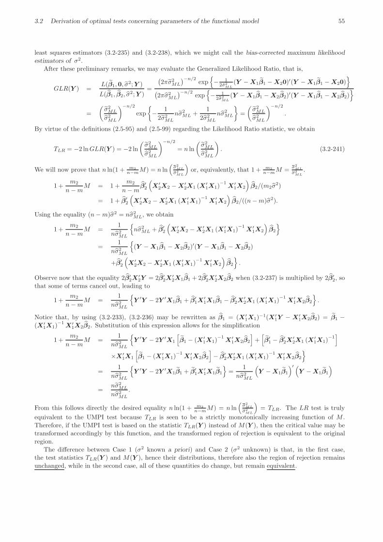
3.2 Derivation of optimal tests concerning parameters of the functional model 55
least squares estimators (3.2-235) and (3.2-238), which we might call the bias-corrected maximum likelihood
estimators of σ2.After these preliminary remarks, we may evaluate the Generalized Likelihood Ratio, that is,
GLR(Y ) =L(β1,0, σ2; Y )
L(β1, β2, σ2; Y )
=
(2πσ2
ML
)−n/2 exp{− 1
2�σ2ML
(Y − X1β1 − X20)′(Y − X1β1 − X20)}
(2πσ2
ML
)−n/2 exp{− 1
2�σ2ML
(Y − X1β1 − X2β2)′(Y − X1β1 − X2β2)}
=(
σ2ML
σ2ML
)−n/2
exp{− 1
2σ2ML
nσ2ML +
12σ2
ML
nσ2ML
}=(
σ2ML
σ2ML
)−n/2
.
By virtue of the definitions (2.5-95) and (2.5-99) regarding the Likelihood Ratio statistic, we obtain
TLR = −2 lnGLR(Y ) = −2 ln(
σ2ML
σ2ML
)−n/2
= n ln(
σ2ML
σ2ML
). (3.2-241)
We will now prove that n ln(1 + m2n−mM) = n ln
(�σ2
ML
�σ2ML
)or, equivalently, that 1 + m2
n−mM = �σ2ML
�σ2ML
.
1 +m2
n − mM = 1 +
m2
n − mβ′
2
(X ′
2X2 − X ′2X1 (X ′
1X1)−1
X ′1X2
)β2/(m2σ
2)
= 1 + β′2
(X ′
2X2 − X ′2X1 (X ′
1X1)−1
X ′1X2
)β2/((n − m)σ2).
Using the equality (n − m)σ2 = nσ2ML, we obtain
1 +m2
n − mM =
1nσ2
ML
{nσ2
ML + β′2
(X ′
2X2 − X ′2X1 (X ′
1X1)−1
X ′1X2
)β2
}=
1nσ2
ML
{(Y − X1β1 − X2β2)′(Y − X1β1 − X2β2)
+β′2
(X ′
2X2 − X ′2X1 (X ′
1X1)−1
X ′1X2
)β2
}.
Observe now that the equality 2β′2X
′2Y = 2β′
2X′2X1β1 + 2β′
2X′2X2β2 when (3.2-237) is multiplied by 2β′
2, sothat some of terms cancel out, leading to
1 +m2
n − mM =
1nσ2
ML
{Y ′Y − 2Y ′X1β1 + β′
1X′1X1β1 − β′
2X′2X1 (X ′
1X1)−1
X ′1X2β2
}.
Notice that, by using (3.2-233), (3.2-236) may be rewritten as β1 = (X ′1X1)−1(X ′
1Y − X ′1X2β2) = β1 −
(X ′1X1)
−1X ′
1X2β2. Substitution of this expression allows for the simplification
1 +m2
n − mM =
1nσ2
ML
{Y ′Y − 2Y ′X1
[β1 − (X ′
1X1)−1
X ′1X2β2
]+[β′
1 − β′2X
′2X1 (X ′
1X1)−1]
×X ′1X1
[β1 − (X ′
1X1)−1
X ′1X2β2
]− β′
2X′2X1 (X ′
1X1)−1
X ′1X2β2
}=
1nσ2
ML
{Y ′Y − 2Y ′X1β1 + β′
1X′1X1β1
}=
1nσ2
ML
(Y − X1β1
)′ (Y − X1β1
)=
nσ2ML
nσ2ML
.
From this follows directly the desired equality n ln(1 + m2n−mM) = n ln
(�σ2
ML
�σ2ML
)= TLR. The LR test is truly
equivalent to the UMPI test because TLR is seen to be a strictly monotonically increasing function of M .Therefore, if the UMPI test is based on the statistic TLR(Y ) instead of M(Y ), then the critical value may betransformed accordingly by this function, and the transformed region of rejection is equivalent to the originalregion.
The difference between Case 1 (σ2 known a priori) and Case 2 (σ2 unknown) is that, in the first case,the test statistics TLR(Y ) and M(Y ), hence their distributions, therefore also the region of rejection remainsunchanged, while in the second case, all of these quantities do change, but remain equivalent.

56 3 THEORY AND APPLICATIONS OF MISSPECIFICATION TESTS IN THE NORMAL GMM
Part 2: From the log-likelihood function
L(β1, β2, σ2; Y ) = ln
[(2πσ2
)−n2 exp
{− 1
2σ2(Y − X1β1 − X2β2)′(Y − X1β1 − X2β2)
}]= −n
2ln(2πσ2) − 1
2σ2(Y − X1β1 − X2β2)′(Y − X1β1 − X2β2).
of the observation model (including both H0 and H1), the log-likelihood score is derived as
S(β1, β2, σ2; Y ) =
⎡⎢⎢⎢⎢⎣∂L(β1, β1, σ
2; Y )∂β1
∂L(β1, β1, σ2; Y )
∂β2∂L(β1, β1, σ
2; Y )∂σ2
⎤⎥⎥⎥⎥⎦ =
⎡⎢⎢⎢⎣1
σ2 X ′1 (Y − X1β1 − X2β2)
1σ2 X ′
2 (Y − X1β1 − X2β2)
− n2σ2 + 1
2σ4 (Y − X1β1 − X2β2)′ (Y − X1β1 − X2β2)
⎤⎥⎥⎥⎦ .
If U = Y − X1β1 − X2β2 denote the residuals, the Hessian and the information matrix read
H(β1, β2, σ2; Y ) =
⎡⎢⎢⎢⎢⎢⎣∂2L(β1, β2, σ
2; Y )∂β1∂β′
1
∂2L(β1, β2, σ2; Y )
∂β1∂β′2
∂2L(β1, β2, σ2; Y )
∂β1∂σ2
∂2L(β1, β2, σ2; Y )
∂β2∂β′1
∂2L(β1, β2, σ2; Y )
∂β2∂β′2
∂2L(β1, β2, σ2; Y )
∂β2∂σ2
∂2L(β1, β2, σ2; Y )
∂σ2∂β1
∂2L(β1,β2,σ2;Y )
∂σ2∂β2
∂2L(β1, β2, σ2; Y )
∂σ2∂σ2
⎤⎥⎥⎥⎥⎥⎦
=
⎡⎢⎢⎢⎣− 1
σ2 X ′1X1 − 1
σ2 X ′1X2 − 1
σ4 X ′1U
− 1σ2 X ′
2X1 − 1σ2 X ′
2X2 − 1σ4 X ′
2U
− 1σ4 U ′X1 − 1
σ4 U ′X2n
2σ4 − 1σ6 U ′U
⎤⎥⎥⎥⎦and
I(β1, β2, σ2; Y ) = E
{−H(β1, β2, σ2; Y )
}
=
⎡⎢⎢⎢⎣1σ2 X ′
1X11
σ2 X ′1X2
1σ4 X ′
1E{U}1σ2 X ′
2X11
σ2 X ′2X2
1σ4 X ′
2E{U}1
σ4 E{U ′}X11
σ4 E{U ′}X2 − n2σ4 + 1
σ6 E{U ′U}
⎤⎥⎥⎥⎦ =
⎡⎢⎢⎢⎣1
σ2 X ′1X1
1σ2 X ′
1X2 01
σ2 X ′2X1
1σ2 X ′
2X2 0
0 0 n2σ4
⎤⎥⎥⎥⎦ ,
where E{U} = 0 and E{U ′U} = nσ2 by virtue of the Markov conditions. From the definition of Rao’s Scorestatistic (), we obtain
TRS(Y ) = S ′(β1, β2, σ2; Y )I−1(β1, β2, σ
2; Y )S(β1, β2, σ2; Y )
=
⎡⎢⎢⎢⎣0
1�σ2
MLX ′
2U
0
⎤⎥⎥⎥⎦′ ⎡⎢⎢⎢⎣
1�σ2
MLX ′
1X11
�σ2ML
X ′1X2 0
1�σ2
MLX ′
2X11
�σ2ML
X ′2X2 0
0 0 n2�σ4
ML
⎤⎥⎥⎥⎦−1 ⎡⎢⎢⎢⎣
01
�σ2ML
X ′2U
0
⎤⎥⎥⎥⎦=
1σ2
ML
U ′X2(X ′2X2)(−1)X ′
2U
= U ′X2
(X ′
2X2 − X ′2X1(X ′
1X1)−1X ′1X2
)−1X ′
2U/σ2ML.
as proposed in (3.2-231). To prove (3.2-232), rewrite TRS as
TRS(Y ) =1
σ2ML
(Y − X1β1
)′X2N
(−1)22 X ′
2
(Y − X1β1
)=
1σ2
ML
(X ′
2Y − X ′2X1β1
)′N
(−1)22
(X ′
2Y − X ′2X1β1
),
substitute (3.2-233) for β1, that is,
TRS(Y ) =1
σ2ML
(X ′
2Y − X ′2X1(X ′
1X1)−1X ′1Y)′
N(−1)22
(N
(−1)22
)−1
N(−1)22
(X ′
2Y − X ′2X1(X ′
1X1)−1X ′1Y).

3.2 Derivation of optimal tests concerning parameters of the functional model 57
Substitution of β2 as given in (3.2-201) yields
TRS(Y ) =1
σ2ML
β′2
(N
(−1)22
)−1
β2.
From Part 1 of the current proof, we already know that 1 + m2n−mM(Y ) = σ2
ML/σ2ML. Isolation of σ2
ML andsubstitution into TRS then results in
TRS(Y ) =β′
2
(N
(−1)22
)−1
β2
σ2ML
(1 + m2
n−mM) .
Using the relationship (n−m)σ2 = nσ2ML between the least squares and the maximum likelihood estimator for
σ2, we obtain
TRS(Y ) =β′
2
(N
(−1)22
)−1
β2
n−mn σ2
(1 + m2
n−mM(Y )) =
nn−m β′
2
(N
(−1)22
)−1
β2/σ2
1 + m2n−mM(Y )
= nm2
n−mM(Y )1 + m2
n−mM(Y ).
As with the relationship between the statistics TLR and M , established in Part 1 of this proof, we see that thestatistic TRS is a strictly monotonically increasing function of M . Therefore, the UMPI test (3.2-159) may bebased upon TRS instead of M if the critical value is transformed according to (3.2-232). In this sense, we saythat Rao’s Score test is equivalent to the UMPI test. If the true value of σ2 is known a priori, then Proposition3.5 states that the statistics TRS and M , hence their distributions, and therefore the corresponding criticalregions are identical.

58 3 THEORY AND APPLICATIONS OF MISSPECIFICATION TESTS IN THE NORMAL GMM
3.3 Application 1: Testing for outliers
Consider the Gauss-Markov model
Y = Xβ + Z∇ + U , (3.3-242)
Σ = Σ{U} = σ2I, (3.3-243)
where Xβ represents the deterministic trend model underlying observations Y , and where Z∇ denotes anadditional mean shift model . Both design matrices X ∈ R
n×m1 and Z ∈ Rn×m2 are assumed to be known
and of full rank. The mean shift model takes its simplest form if Z is a vector with zeros in the components1, . . . , i − 1, i + 1, . . . , n and a one in the i-th component, that is,
Z = [ 0 · · · 0 1 0 · · · 0 ]′ . (3.3-244)
Then, the mean shift parameter ∇ may be viewed as a single additive outlier or gross error affecting obser-vation Yi. If a model for multiple outliers is desired, then Z is simply expanded by additional columns. A testfor a single (or multiple) outlier(s) may then be based on the hypotheses
H0 : ∇ = 0 versus H1 : ∇ �= 0. (3.3-245)
Clearly, if H0 is true, then no outliers are present in the data, and if H1 is true, then at least one outlier ispresent.
If the errors U follow a normal distribution with expectation E{U} = 0 , then we may rewrite the Gauss-Markov model (3.3-242)+(3.3-243) as
Y ∼ N(Xβ + Z∇, σ2I). (3.3-246)
This observation model, together with the hypotheses (3.3-245), is seen to constitute a natural problem of testing
the significance of additional parameters ∇ according to (3.2-167)+(3.2-168) or (3.2-198)+(3.2-199), dependingon whether the variance factor σ2 is known or unknown a priori. We will investigate both case separately insubsequent sections 3.3.1 and 3.3.2.
Example 3.1: Linear regression with a group of adjacent outliers. The following dataset (Fig. 3.1)has been analyzed by Rousseeuw and Leroy (2003, p. 26) in the context of outlier testing and robust parameterestimation. As the observations between 1964 and 1969 are seen to clearly mismatch the rest of the data,which may be approximated reasonably well by a straight line, we could take this fact into consideration byintroducing additional mean shift parameters ∇1, . . . ,∇6.
1950 1955 1960 1965 1970−5
0
5
10
15
20
25
Year
Num
ber
of C
alls
(x
10 M
io.)
Figure 3.1. Linear regression model with six additional adjacent mean shift parameters.

3.3 Application 1: Testing for outliers 59
The functional model may be written according to (3.3-242), that is,⎡⎢⎢⎢⎢⎢⎢⎢⎢⎢⎢⎢⎢⎢⎢⎢⎢⎢⎢⎢⎢⎢⎢⎢⎢⎢⎢⎢⎢⎢⎢⎢⎢⎣
Y1
...
Y14
Y15
Y16
Y17
Y18
Y19
Y20
Y21
...
Y24
⎤⎥⎥⎥⎥⎥⎥⎥⎥⎥⎥⎥⎥⎥⎥⎥⎥⎥⎥⎥⎥⎥⎥⎥⎥⎥⎥⎥⎥⎥⎥⎥⎥⎦
=
⎡⎢⎢⎢⎢⎢⎢⎢⎢⎢⎢⎢⎢⎢⎢⎢⎢⎢⎢⎢⎢⎢⎢⎢⎢⎢⎢⎢⎢⎢⎢⎢⎢⎣
1 1950...
...
1 1963
1 1964
1 1965
1 1966
1 1967
1 1968
1 1969
1 1970...
...
1 1973
⎤⎥⎥⎥⎥⎥⎥⎥⎥⎥⎥⎥⎥⎥⎥⎥⎥⎥⎥⎥⎥⎥⎥⎥⎥⎥⎥⎥⎥⎥⎥⎥⎥⎦
⎡⎣ β1
β2
⎤⎦+
⎡⎢⎢⎢⎢⎢⎢⎢⎢⎢⎢⎢⎢⎢⎢⎢⎢⎢⎢⎢⎢⎢⎢⎢⎢⎢⎢⎢⎢⎢⎢⎢⎢⎣
0 0 0 0 0 0...
......
......
...
0 0 0 0 0 0
1 0 0 0 0 0
0 1 0 0 0 0
0 0 1 0 0 0
0 0 0 1 0 0
0 0 0 0 1 0
0 0 0 0 0 1
0 0 0 0 0 0...
......
......
...
0 0 0 0 0 0
⎤⎥⎥⎥⎥⎥⎥⎥⎥⎥⎥⎥⎥⎥⎥⎥⎥⎥⎥⎥⎥⎥⎥⎥⎥⎥⎥⎥⎥⎥⎥⎥⎥⎦
⎡⎢⎢⎢⎢⎢⎢⎢⎢⎢⎢⎢⎢⎢⎣
∇1
∇2
∇3
∇4
∇5
∇6
⎤⎥⎥⎥⎥⎥⎥⎥⎥⎥⎥⎥⎥⎥⎦+
⎡⎢⎢⎢⎢⎢⎢⎢⎢⎢⎢⎢⎢⎢⎢⎢⎢⎢⎢⎢⎢⎢⎢⎢⎢⎢⎢⎢⎢⎢⎢⎢⎢⎣
U1
...
U14
U15
U16
U17
U18
U19
U20
U21
...
U24
⎤⎥⎥⎥⎥⎥⎥⎥⎥⎥⎥⎥⎥⎥⎥⎥⎥⎥⎥⎥⎥⎥⎥⎥⎥⎥⎥⎥⎥⎥⎥⎥⎥⎦�
3.3.1 Baarda’s test
If the true value of the variance factor in (3.3-243) is known to take the a priori value σ2 = σ20 , then Proposition
3.3 guarantees that there exists a UMPI test for the outlier test problem
Y ∼ N(Xβ + Z∇, σ20I). (3.3-247)
and hypotheses (3.3-245). According to (3.2-158), the UMPI test is given by
φ(y) =
⎧⎨⎩ 1, if M(y) > kχ2(m2)1−α ,
0, if M(y) < kχ2(m2)1−α ,
(where m2 denotes the number of modeled outliers) with statistic
M(Y ) = ∇′(Z ′Z − Z ′X (X ′X)−1
X ′Z)
∇/σ20 (3.3-248)
following from (3.2-169), and least squares estimator
∇ =(Z ′Z − Z ′X (X ′X)−1
X ′Z)−1
Z ′Y −(Z ′Z − Z ′X (X ′X)−1
X ′Z)−1
Z ′X (X ′X)−1X ′Y
(3.3-249)
for the outliers ∇ corresponding to (3.2-180). This test is called Baarda’s test (Baarda, 1967, 1968). We mayrewrite (3.3-249) in the more common form
∇ =(Z ′(I − X (X ′X)−1
X ′)
Z)−1
Z ′(I − X (X ′X)−1
X ′)
Y (3.3-250)
=(Z ′Q{U}Z
)−1
Z ′Q{U}Y (3.3-251)
where Q{U} evidently denotes the cofactor matrix of residuals U = Y −Xβ in the outlier-free Gauss-Markovmodel
Y = Xβ + U , (3.3-252)
Σ = Σ{U} = σ2I. (3.3-253)
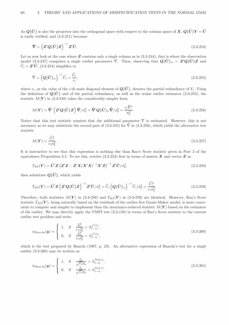
60 3 THEORY AND APPLICATIONS OF MISSPECIFICATION TESTS IN THE NORMAL GMM
As Q{U} is also the projector into the orthogonal space with respect to the column space of X, Q{U}Y = U
is easily verified, and (3.3-251) becomes
∇ =(Z ′Q{U}Z
)−1
Z ′U . (3.3-254)
Let us now look at the case where Z contains only a single column as in (3.3-244), that is where the observationmodel (3.3-247) comprises a single outlier parameter ∇. Then, observing that Q{U}ii = Z ′Q{U}Z andUi = Z ′U , (3.3-254) simplifies to
∇ =(Q{U}ii
)−1
Ui =Ui
ri, (3.3-255)
where ri, as the value of the i-th main diagonal element of Q{U}, denotes the partial redundancy of Yi. Usingthe definition of Q{U} and of the partial redundancy, as well as the scalar outlier estimator (3.3-255), thestatistic M(Y ) in (3.3-248) takes the considerably simpler form
M(Y ) = ∇′(Z ′Q{U}Z
)∇/σ2
0 = ∇′Q{U}ii∇/σ20 =
ri∇2
σ20
. (3.3-256)
Notice that this test statistic requires that the additional parameter ∇ is estimated. However, this is notnecessary as we may substitute the second part of (3.3-255) for ∇ in (3.3-256), which yields the alternative teststatistic
M(Y ) =U2
i
riσ20
. (3.3-257)
It is instructive to see that this expression is nothing else than Rao’s Score statistic given in Part 2 of theequivalence Proposition 3.5. To see this, rewrite (3.2-224) first in terms of matrix X and vector Z as
TRS(Y ) = U ′Z(Z ′Z − Z ′X(X ′X)−1X ′Z
)−1Z ′U/σ2
0 , (3.3-258)
then substitute Q{U}, which yields
TRS(Y ) = U ′Z(Z ′Q{U}Z
)−1
Z ′U/σ20 = Ui
(Q{U}ii
)−1
Ui/σ20 =
U2i
riσ20
. (3.3-259)
Therefore, both statistics M(Y ) in (3.3-256) and TRS(Y ) in (3.3-259) are identical. However, Rao’s Scorestatistic TRS(Y ), being naturally based on the residuals of the outlier-free Gauss-Makov model, is more conve-nient to compute and simpler to implement than the invariance-reduced statistic M(Y ) based on the estimatorof the outlier. We may directly apply the UMPI test (3.2-158) in terms of Rao’s Score statistic to the currentoutlier test problem and write
φBaarda(y) =
⎧⎪⎨⎪⎩1, if u2
i
riσ20
> kχ2(1)1−α ,
0, if u2i
riσ20
< kχ2(1)1−α ,
(3.3-260)
which is the test proposed by Baarda (1967, p. 23). An alternative expression of Baarda’s test for a singleoutlier (3.3-260) may be written as
φBaarda(y) =
⎧⎪⎨⎪⎩1, if ui√
riσ0> k
N(0,1)1−α ,
0, if ui√riσ0
< kN(0,1)1−α .
(3.3-261)

3.3 Application 1: Testing for outliers 61
Example 3.2: Testing for multiple outliers. The Gravity Dataset given in Appendix 6.2, which has beenkindly communicated by Dr. Diethard Ruess, consists of n = 91 gravity differences between the old and thenew Austrian gravity network (Osterreichisches Schweregrundnetz, OSGN). To approximate this data, we usethe polynomial
yi = β1 + β2φi + β3λi (i = 1, . . . , 91) (3.3-262)
as functional model, where φi denote the latitudes and λi the longitudes (in decimal degrees). The data isassumed to be uncorrelated and of constant standard deviation σ0 = 0.08 mgal. Schuh (2006b) suggested thatthe observations y3, y6, y10, y42, y45, y78, y87, y89 are outliers. To test the data against this hypothesis, we addeight additional shift parameters ∇1, . . . ,∇8 to the functional model (3.3-262). The observation equations thenread
yi = β1 + β2φi + β3λi + ui (i = 1, 2)y3 = β1 + β2φ3 + β3λ3 + ∇1 + u1
yi = β1 + β2φi + β3λi + ui (i = 4, 5)y6 = β1 + β2φ6 + β3λ6 + ∇2 + u6
yi = β1 + β2φi + β3λi + ui (i = 7, 8, 9)y10 = β1 + β2φ10 + β3λ10 + ∇3 + u10
yi = β1 + β2φi + β3λi + ui (i = 11, . . . , 41)y42 = β1 + β2φ42 + β3λ42 + ∇4 + u42
yi = β1 + β2φi + β3λi + ui (i = 43, . . . , 44)y45 = β1 + β2φ45 + β3λ45 + ∇5 + u45
yi = β1 + β2φi + β3λi + ui (i = 46, . . . , 77)y78 = β1 + β2φ78 + β3λ78 + ∇6 + u78
yi = β1 + β2φi + β3λi + ui (i = 79, . . . , 86)y87 = β1 + β2φ87 + β3λ87 + ∇7 + u87
yi = β1 + β2φi + β3λi + ui (i = 88)y89 = β1 + β2φ89 + β3λ89 + ∇8 + u89
yi = β1 + β2φi + β3λi + ui (i = 90, 91)
Hence, the observation model is given as in (3.3-247) with (rounded) design matrices
X =
⎡⎢⎢⎢⎢⎢⎢⎢⎢⎢⎢⎢⎢⎢⎢⎢⎢⎢⎢⎢⎢⎢⎢⎢⎢⎢⎢⎣
1 48.1710 16.31681 48.2328 16.33731 48.3120 16.43081 48.7192 16.30331 48.5125 16.62171 48.6927 16.87071 48.3620 15.40381 48.1980 14.52801 48.1257 14.87881 48.1593 15.10101 48.2242 15.3580...
......
1 47.4573 09.64071 47.4307 09.75631 47.1325 10.1218
⎤⎥⎥⎥⎥⎥⎥⎥⎥⎥⎥⎥⎥⎥⎥⎥⎥⎥⎥⎥⎥⎥⎥⎥⎥⎥⎥⎦
, Z =
⎡⎢⎢⎢⎢⎢⎢⎢⎢⎢⎢⎢⎢⎢⎢⎢⎢⎢⎢⎢⎢⎢⎢⎢⎢⎢⎢⎣
0 0 0 0 0 0 0 00 0 0 0 0 0 0 01 0 0 0 0 0 0 00 0 0 0 0 0 0 00 0 0 0 0 0 0 00 1 0 0 0 0 0 00 0 0 0 0 0 0 00 0 0 0 0 0 0 00 0 0 0 0 0 0 00 0 1 0 0 0 0 00 0 0 0 0 0 0 0...
......
......
......
...0 0 0 0 0 0 0 10 0 0 0 0 0 0 00 0 0 0 0 0 0 0
⎤⎥⎥⎥⎥⎥⎥⎥⎥⎥⎥⎥⎥⎥⎥⎥⎥⎥⎥⎥⎥⎥⎥⎥⎥⎥⎥⎦
.
Estimation of the mean shift parameters according to (3.3-249) yields
∇ = [−0.3024, 0.1331, −0.1608, −0.1944, −0.2100, 0.1703, −0.2756, 0.1899]′,
and the test statistic (3.3-248) takes the value M(y) = 54.46, which is larger than kχ2(8)0.95 = 15.51. Thus, Baarda’s
test rejects H0, i.e. vector of outlier parameters is significant. To carry out this test, we could also compute Rao’sScore statistic (3.3-258) via the estimated residuals u = y − Xβ based on the restricted parameter estimates
β = (X ′X)−1X ′y = [13.8830, 0.0186, 0.0188]′.
This gives the identical result TRS = 54.46. �

62 3 THEORY AND APPLICATIONS OF MISSPECIFICATION TESTS IN THE NORMAL GMM
3.3.2 Pope’s test
If, in contrast to the situation in Section 3.3.1, the variance factor is unknown a priori, then we must applyPart 1 of Proposition 3.4, which states that there exists a UMPI test for the outlier test problem
Y ∼ N(Xβ + Z∇, σ2I). (3.3-263)
with hypotheses (3.3-245). According to (3.2-159), the UMPI test is given by
φ(y) =
{1, if M(y) > k
F (m2,n−m)1−α ,
0, if M(y) < kF (m2,n−m)1−α ,
with statistic
M(Y ) = ∇′(Z ′Z − Z ′X (X ′X)−1
X ′Z)
∇/(m2σ2) (3.3-264)
following from (3.2-200). The least squares estimator for the outliers ∇, rearranged as in (3.3-251) by using theresiduals U = Y − Xβ of the non-extended model,
∇ =(Z ′Q{U}Z
)−1
Z ′Q{U}Y (3.3-265)
follow from (3.2-213) and the least squares estimator
σ2 = U ′U/(n − m) (3.3-266)
for σ2 from (3.2-214), where the residuals
U =(I − X (X ′X)−1
X ′)(
Y − Z∇)
(3.3-267)
of the extended model are given by (3.2-203). If only a single outlier is modeled, in other words, if Z has onlym2 = 1 columns, then (3.3-265) becomes
∇ =Ui
ri, (3.3-268)
which is identical to (3.3-255) for Baarda’s test. The test statistic (3.3-264) then simplifies to
M(Y ) =ri∇2
σ2. (3.3-269)
The only difference between the statistics (3.3-257) and (3.3-269) is that the former is based on the a priori
variance factor σ20 and the latter on the estimator of the variance factor in the extended model. As the non-
extended model is easier to adjust, it is more convenient to apply Rao’s Score statistic whose general form(3.2-231) is simplified for the current test problem as follows:
TRS(Y ) = U ′Z(Z ′Z − Z ′X(X ′X)−1X ′Z
)−1Z ′U/σ2
ML =U2
i
riσ2ML
=nU2
i
(n − m)riσ2. (3.3-270)
The UMPI test (3.2-159) in terms of Rao’s Score statistic takes the expression
φPope(y) =
⎧⎪⎨⎪⎩1, if nu2
i
(n − m)riσ2 > k
F (1,n−m)1−α ,
0, if nu2i
(n − m)riσ2 < k
F (1,n−m)1−α ,
(3.3-271)
which was proposed in Pope (1976, p. 17). Pope’s test is sometimes written in a square-root version of(3.3-271) as
φPope(y) =
⎧⎪⎨⎪⎩1, if ui√
riσ> k
τ(1,n−m)1−α ,
0, if ui√riσ
< kτ(1,n−m)1−α ,
(3.3-272)
where kτ(1,n−m)1−α denotes the critical value of the Tau distribution. Koch (1999, p. 303) shows that the Tau
distribution is a function of the F distribution, and that both forms (3.3-271) and (3.3-272) of Pope’s test areidentical.

3.4 Application 2: Testing for extensions of the functional model 63
3.4 Application 2: Testing for extensions of the functional model
Suppose that we want to approximate given observables Y by a Gauss-Markov model
Yi =p∑
j=0
Bj(xi)aj + Ui, Σ{U} = σ2I, (3.4-273)
where Bj(xi) denote base functions evaluated at known, not necessarily equidistant, nodes or locations xi
(i = 1, . . . , n) and β = [ a0, . . . , ap ] the unknown parameters. Frequently used base functions Bj (j = 0, . . . , p)are, for instance, polynomials, trigonometric functions, or spherical harmonics. Let us further assume thatthe errors Ui (i = 1, . . . , n) are uncorrelated, homoscedastic, and normally distributed variables. If they werecorrelated and/or heteroscedastic with weight matrix P , then we would preprocess the observation equationsby decorrelation and/or homogenization as in Sect. 3.2.3.
In a practical situation with insufficient knowledge about the physical or geometrical relationship betweenthe data and the nodes, it might not be clear how high the degree m of, for example, a polynomial expansionshould be. Let us say we believe that the degree of the expansion should be specified by p1, but we would liketo check whether the base function Bp2 with p2 = p1 + 1 should be added to the model. One approach wouldbe to estimate the parameters of the model (3.4-273) up to degree p2 and to perform a significance test of theparameter ap2 . If ap2 turns out to be insignificant, then we carry out a new adjustment of the model (3.4-273)with degree p1.
If we define β1 := [ a0, . . . , ap1 ] and β2 := ap2 , and if we let X1 and X2 contain the values of the basefunctions evaluated at the locations, then we may rewrite (3.4-273) as
y = X1β1 + X2β2 + u, Σ{U} = σ2I, (3.4-274)
and the significance test of ap2 is about the hypotheses
H0 : β2 = 0 versus H1 : β2 �= 0.
As this problem is one of testing the significance of m2 = 1 additional parameter β2 with either known orunknown variance factor, the UMPI test (3.2-158) or (3.2-159) is based on either the statistic
M(Y ) = β′2
(X ′
2X2 − X ′2X1(X ′
1X1)−1X1X2
)β2/σ2
0
or
M(Y ) = β′2
(X ′
2X2 − X ′2X1(X ′
1X1)−1X1X2
)β2/(m2σ
2)
by virtue of (3.2-169) and (3.2-200) in Propositions 3.4/3.5.If however, on the grounds of prior information, we favor the model up to degree p1 over the model up
to degree p2, then it seems more reasonable to adjust the smaller model (with p1) first, and to estimate theadditional parameters only after they have been verified to be significant. To imlement such a significance test,which is a reversed version of the significance test based on M(Y ), we may use Rao’s Score statistic
TRS(Y ) = U ′X2
(X ′
2X2 − X ′2X1(X ′
1X1)−1X ′1X2
)−1X ′
2U/σ20
(if the variance factor is known) or
TRS(Y ) = U ′X2
(X ′
2X2 − X ′2X1(X ′
1X1)−1X ′1X2
)−1X ′
2U/σ2ML
(if the variance factor must be estimated) as defined in (3.2-224) and (3.2-231). These statistics are based onthe estimated residuals of the Gauss-Markov model (3.4-274) with the restriction β2 = 0, which is equivalent tothe ordinary Gauss-Markov model
y = X1β1 + u, Σ{U} = σ2I. (3.4-275)
Rao’s Score statistics for testing the significance of additional base functions are merely a generalization ofBaarda’s and Pope’s statistic for testing the significance of outliers. This fact has already been pointed outby Jaeger et al. (2005, Section 5.4.5.5) in the context of testing the significance of additional transformationparameters.

64 3 THEORY AND APPLICATIONS OF MISSPECIFICATION TESTS IN THE NORMAL GMM
Example 3.3: Testing for extension of a two-dimensional polynomial. We will demonstrate the twodifferent approaches to significance testing of additional model parameters by further analyzing the GravityDataset from Example 3.2. For simplicity, the outlying observations y3, y6, y10, y42, y45, y78, y87, y89 will not beused, i.e. the corresponding rows are eliminated from y and X. Now, we could consider
Yi = a0 + φia1 + λia2 (i = 1, . . . , 83) (3.4-276)
as the model we favor under H0, and the extension to degree 2
Yi = a0 + φia1 + λia2 + φ2i a3 + φiλia4 + λ2
i a5 (i = 1, . . . , 83) (3.4-277)
as an alternative model specification. This model is simply a two-dimensional polynomial version of the model in(3.4-273). We see that the null model (3.4-276) is obtained from the extended model (3.4-277) if the additionalparameters a3, a4, a5 are restricted to zero. To test whether the null model is misspecified, we will rewritethe extended model in the form (3.4-274) with σ0 = 0.08 known a priori. In the present example, we defineβ1 := [a0, a1, a2]′ and β2 := [a3, a4, a5]′, and use the hypotheses H0 : β2 = 0 versus H1 : β2 �= 0. The designmatrix X1 is obtained from X in Example 3.2 by deleting rows as described above.
X1 =
⎡⎢⎢⎢⎢⎢⎢⎢⎢⎢⎢⎢⎢⎢⎢⎢⎢⎢⎢⎣
1 48.1710 16.31681 48.2328 16.33731 48.7192 16.30331 48.5125 16.62171 48.3620 15.40381 48.1980 14.52801 48.1257 14.87881 48.2242 15.3580...
......
1 47.4307 09.75631 47.1325 10.1218
⎤⎥⎥⎥⎥⎥⎥⎥⎥⎥⎥⎥⎥⎥⎥⎥⎥⎥⎥⎦
, X2 =
⎡⎢⎢⎢⎢⎢⎢⎢⎢⎢⎢⎢⎢⎢⎢⎢⎢⎢⎢⎣
2320.4452 785.9982 266.23912326.4062 787.9959 266.90852373.5572 794.2848 265.79872353.4627 806.3586 276.27982338.8830 744.9602 237.27812323.0472 700.2205 211.06282316.0798 716.0538 221.37972325.5703 740.6268 235.8682
......
...2249.6681 462.7494 95.18602221.4726 477.0673 102.4515
⎤⎥⎥⎥⎥⎥⎥⎥⎥⎥⎥⎥⎥⎥⎥⎥⎥⎥⎥⎦Notice the close similarity of this testing problem with the problem of testing for outliers in Example 3.2. Theonly difference is that the additional parameters β2 appear in every single observation equations while eachmean shift parameter in ∇ affects only a single observation. Here we could analogously estimate β2 as in(3.2-170) and then compute the value of the test statistic (3.2-169). This gives
β2 =(X ′
2X2 − X ′2X1(X ′
1X1)−1X1X2
)−1X ′
2(I − X1 (X ′1X1)
−1X ′
1)y
= [−0.0287, −0.0170, −0.0044]′
and
M(y) = β′2
(X ′
2X2 − X ′2X1(X ′
1X1)−1X1X2
)β2/σ2
0 = 7.74,
which is smaller than the critical value kχ2(3)0.95 = 7.81. This test again yields the same result if only the parameters
β1 of the null model are estimated and if then the corresponding residuals u = y−X1β1 are used to determinethe value of Rao’s Score statistic (3.2-224). This would result in
β1 = (X ′1X1)−1X ′
1y = [14.1459, 0.0122, 0.0224]
and
TRS(y) = u′X2
(X ′
2X2 − X ′2X1(X ′
1X1)−1X ′1X2
)−1X ′
2u/σ20 = 7.74.
The values in β1 differ slightly from those in β from Example 3.2 as a consequence of deleting observations.Hence, we could not reject the null model, i.e. the joint set of additional parameters could not be proven to besignificant.

3.5 Application 3: Testing for point displacements 65
3.5 Application 3: Testing for point displacements
In Meissl (1982, Sect. 5.4) the following test problem is discussed. A leveling network has been measured twice(see Fig. 3.2), and the question is whether three of the points (7,8, and 9), which are located on a dam, changedin heights between both measurement campaigns. Point 1 has a fixed height, and the heights of the points 2,3, 4, 5, and 6 are assumed to be unknown, but constant over time.
1 2 3
45
6
78
9
1 2 3
45
6
7‘8‘
9‘
Fig. 3.2 A leveling network observed in a first campaign (left) and a second campaign (right) later in time.
The general structure of the observation model is specified as
y = Xβ + u, Σ{U} = σ2I, (3.5-278)
where the functional model comprises n = 34 leveling observations y (i.e. observed height differences) withunknown accuracy σ2 (see Appendix 6.1 for the numerical values). To allow for height displacements, theparameter vector
β = [ H2, H3, H4, H5, H6, H7, H8, H9, H7′ , H8′ , H9′ ]′
contains the set of dam heights (H7, H8, H9) regarding the first campaign and the set (H7′ , H8′ , H9′) for thepossibly different points modeled with respect to the second campaign. Let, for example, y5 represent theobserved height difference between points 2 and 8 (made in the first campaign) and y24 the observed heightdifference between points 2 and 8’ (made in the second campaign). Then, the corresponding observationequations read
y5 = H8 − H2 + u5,
y24 = H8′ − H2 + u24,
and the corresponding rows of the design matrix are given by
X5 = [−1, 0, 0, 0, 0, 0, 1, 0, 0, 0, 0 ],
X24 = [−1, 0, 0, 0, 0, 0, 0, 0, 0, 1, 0 ].
The mathematical formulation of the above question, whether the points 7, 8, and 9 shifted significantly, isgiven by the null hypothesis H7′ = H7, H8′ = H8, H8′ = H8 versus the alternative hypothesis H7′ �= H7, H8′ �=H8, H8′ �= H8, or in matrix notation by
H0 : Hβ = 0 versus H1 : Hβ �= 0
with
H =
⎡⎣ 0 0 0 0 0 −1 0 0 +1 0 00 0 0 0 0 0 −1 0 0 +1 00 0 0 0 0 0 0 −1 0 0 +1
⎤⎦ .
For this testing problem, Meissl (1982) gives the statistic
M(Y ) = (Hβ)′(H(X ′X)−1H ′)−1
(Hβ)/(3σ2), (3.5-279)

66 3 THEORY AND APPLICATIONS OF MISSPECIFICATION TESTS IN THE NORMAL GMM
which is distributed as F (3, n − m), because the model has three restrictions.As an additional result however, we may conclude from Proposition 3.4(3) that this statistic leads to an
optimal invariant test, because the testing problem is of the form (3.2-217) + (3.2-218) with P = I and w = 0.Consequently, using the test statistic (3.2-216) with m2 = 3 and least squares estimates
β = (X ′X)−1X ′y, (3.5-280)
u = y − Xβ, (3.5-281)
σ2 = u′u/(n − m) (3.5-282)
according to (3.2-219) - (3.2-221) leads to the UMPI test as given in (3.2-159). With the given numerical valuesin Appendix 6.1, the test statistic takes the value M(y) = 53.61, which exceeds for instance the critical valuek
F (3,23)0.95 = 3.03. Therefore, we conclude that the data shows significant evidence for a shift in height.
We will now demonstrate how this testing problem is reparameterized as in 3.2.1. Notice first that thefunctional model may be partitioned into y = X1β1 + X2β2 + u with
β1 = [ H2, H3, H4, H5, H6, H7, H8, H9 ]′,
β2 = [ H7′ , H8′ , H9′ ]′
and, regarding observations y5 and y24,
X5,1 = [−1, 0, 0, 0, 0, 0, 1, 0 ], X5,2 = [ 0, 0, 0 ],
X24,1 = [−1, 0, 0, 0, 0, 0, 0, 0 ], X24,2 = [ 0, 1, 0 ].
Now, if we use
∆H7 := H7′ − H7
∆H8 := H8′ − H8
∆H9 := H9′ − H9,
i.e. the transformed quantities Hβ, as parameters instead of H7′ , H8′ , and H9′ , then the new parameter vectorreads
β(r) = [ β′(r)1 , β
′(r)2 ]′ = [ H2, H3, H4, H5, H6, H7, H8, H9, ∆H7, ∆H8, ∆H9 ]′
with components
β(r)1 = [ H2, H3, H4, H5, H6, H7, H8, H9 ]′,
β(r)2 = [ ∆H7, ∆H8, ∆H9 ]′.
Clearly, the hypotheses
H0 : β(r)2 = 0 versus H1 : β
(r)2 �= 0
in terms of the new parameters are identical to the original hypotheses. To see how the design matrix changes,we first rewrite the observation equations, for instance, with respect to y5 and y24
y5 = H8 − H2 + u5,
y24 = H8′ − H8 + H8 − H2 + u24 = H8 + ∆H8 − H2 + u24.
The corresponding rows of the design matrix with respect to the new parameters β(r) read
X(r)5,1 = [−1, 0, 0, 0, 0, 0, 1, 0 ], X
(r)5,2 = [ 0, 0, 0 ],
X(r)24,1 = [−1, 0, 0, 0, 0, 0, 1, 0 ], X
(r)24,2 = [ 0, 1, 0 ].
We see that β(r)1 = β1, X
(r)5,1 = X5,1, X
(r)5,2 = X5,2, and X
(r)24,2 = X24,2. For the present example these equations
in fact hold for all rows of the design matrix, so that the reparameterized observation model is given by
y = X(r)1 β1 + X2β
(r)2 + u,
Σ = σ2I.

3.5 Application 3: Testing for point displacements 67
According to Proposition 3.4-1, the UMPI test for this reparameterized testing problem is based on the valueof the statistic
M(y) = β′(r)2
(X ′
2X2 − X ′2X
(r)1 (X ′(r)
1 X(r)1 )−1X
′(r)1 X2
)β
(r)2 /(3σ2) (3.5-283)
with estimates
β(r)2 =
(X ′
2X2 − X ′2X
(r)1 (X ′(r)
1 X(r)1 )−1X
′(r)1 X2
)−1
X ′2
(I − X
(r)1 (X ′(r)
1 X(r)1 )−1X
′(r)1
)y, (3.5-284)
u =(I − X
(r)1 (X ′(r)
1 X(r)1 )−1X
′(r)1
)(y − X2β
(r)2
), (3.5-285)
σ2 = u′u/(n − m). (3.5-286)
With the given data, the displacement parameters take the values β(r)2 = [ 0.0044, 0.0047, 0.0056 ]′, and the
test statistic becomes M(y) = 53.61, which is of course the same value as determined above for 3.5-279. Noticethat, as demonstrated in the proof of Proposition 3.4, the quantities M(y), u, and σ2 remain unchanged by thereparameterization of the observation equations. This transformation allows us to apply Proposition 3.6 andcompute the value of Rao’s Score statistic by
TRS(y) = u′X2
(X ′
2X2 − X ′2X
(r)1 (X ′(r)
1 X(r)1 )−1X
′(r)1 X2
)−1
X ′2u/σ2
ML, (3.5-287)
which requires the estimates
β1 = (X ′(r)1 X
(r)1 )−1X
′(r)1 y, (3.5-288)
u = y − X(r)1 β1, (3.5-289)
σ2ML = u′u/n. (3.5-290)
With the given data, we obtain TRS(y) = 29.74. As the relationship between the statistics M and TRS hasbeen shown to be (3.2-232), we may apply this formula to check the validity of the results and to compute thecritical value valid for TRS . We find that
TRS(y) = 34 ·323M(y)
1 + 323M(y)
and kTRS0.95 = 34 ·
323k
F (3,23)0.95
1 + 323k
F (3,23)0.95
= 9.63.
As Rao’s Score statistic is determined under the assumption that H0 is true, the null hypothesis H0 : β(r)2 = 0
acts as a restriction on the Gauss-Markov model, and thus eliminates the parameters β(r)2 from the reparame-
terized observation equations. In other words, if H0 is true, then the Gauss-Markov model with restrictions
y = X(r)1 β1 + X2β
(r)2 + u,
β(r)2 = 0
Σ = σ2I
is equivalent to the Gauss-Markov model
y = X(r)1 β1 + u, Σ = σ2I, (3.5-291)
for which the estimates are given by (3.5-288) - (3.5-290). The main advantage of Rao’s Score statistic TRS in(3.5-287) over M in (3.5-283) is that the restricted estimates β1 are clearly less complex to compute than theunrestricted estimates β
(r)2 . Furthermore, TRS has an advantage over M in (3.5-279), because the restricted
reparameterized Gauss-Markov model (3.5-291) has less unknown parameters to be estimated than the originalmodel (3.5-278).

68 3 THEORY AND APPLICATIONS OF MISSPECIFICATION TESTS IN THE NORMAL GMM
3.6 Derivation of an optimal test concerning the variance factor
So far we have only discussed testing problems concerning the parameters β of the functional model
Y = Xβ + E.
In the current section, we will derive an optimal procedure for testing hypotheses concerning the variance factorσ2 in the stochastic model
Σ = Σ{E} = σ2P−1.
As usual we will assume that the design matrix X ∈ Rn×m is known and of full rank, and that the weight
matrix P ∈ Rn×n is positive definite. If we decompose the weight matrix into P = GG′ as in Section 3.2.3,
then the observations and the design matrix may be transformed into Y (h) := G′Y and X(h) := G′X, whereY (h) has the covariance matrix σ2I.
Let us now consider the problem of testing
H0 : σ2 = σ20 versus H1 : σ2 > σ2
0
in the observation model
Y (h) ∼ N(X(h)β, σ2I).
Such a testing problem arises if we suspect that the given measurement accuracy σ20 is too optimistic.
Proposition 3.1 allows us now to reduce Y (h) to the set of minimally sufficient statistics T (Y (h)) := [β′, σ2]′
with β = (X ′(h)X(h))−1X ′(h)Y (h) and (n−m)σ2 = (Y (h) −X(h)β)′(Y (h) −X(h)β). The reduced observationmodel then reads
β ∼ N(β, σ2(X ′(h)X(h))−1
),
(n − m)σ2 ∼ χ2(n − m) · σ2,
and the hypotheses are still given by
H0 : σ2 = σ20 versus H1 : σ2 > σ2
0
This testing problem is invariant under the group G of translations
g
([β
σ2
])=[
β + a
σ2
](3.6-292)
with a ∈ Rm×1 acting on β. Each of these tranformations will cause a change of distribution from β ∼
N(β, σ2(X ′(h)X(h))−1
)to β + a ∼ N
(β + a, σ2(X ′(h)X(h))−1
), while the second central moment of β and
the distribution of σ2 remain unaffected by these translations. Thus, the induced group G of transformationswithin the parameter domain is given by
g
([β
σ2
])=[
β + a
σ2
]. (3.6-293)
Evidently, neither the parameter space nor the hypotheses are changed under G. Moreover, we see that σ2, ormore conveniently M(Y (h)) := (n−m)σ2 is a maximal invariant under G. From the fact that (n−m)σ2/σ2 ∼χ2(n − m) = G(n−m
2 , 2) (where G stands here for the Gamma distribution) it follows that (n − m)σ2 ∼G(n−m
2 , 2σ2). Thus, the invariant test problem
M(Y ) = (n − m)σ2 ∼ G((n − m)/2, 2σ2)
H0 : σ2 = σ20 versus H1 : σ2 > σ2
0 ,
has one unknown parameter, a one-sided alternative hypothesis, and a test distribution with a monotone densityratio by virtue of Theorem 2.5-2. For this reduced testing problem, Theorem 2.4 gives the UMP test
φ(y) =
{1, if M(y) > k
G((n−m)/2,2σ20)
1−α ,
0, if M(y) < kG((n−m)/2,2σ2
0)1−α ,
=
{1, if (n − m)σ2/σ2
0 > kχ2(n−m)1−α ,
0, if (n − m)σ2/σ20 < k
χ2(n−m)1−α ,
(3.6-294)
which is UMPI for the original problem of testing H0 : σ2 = σ20 against H1 : σ2 > σ2
0 in the observation modelY (h) ∼ N(X(h)β, σ2I). This test is the same as given in Koch (1999, Section 4.2.4), but it was shown here inaddition that (3.6-294) is optimal within the class of all tests with equal power in each direction of β.

69
4 Applications of Misspecification Tests in Generalized Gauss-Markov
models
4.1 Introduction
In this section, we will look at testing problems, where parameters of the distribution or stochastic modelare hypothesized. In each of these problems, the null hypothesis states that the errors are distributed asE ∼ N(0, σ2I), whereas the alternative hypothesis represents one of the following types of model errors:
1. the errors are not uncorrelated, but correlated through an autoregressive process (Section 4.2);
2. the errors are not homoscedastic, but the variance changes according to an additive variance component(Section 4.3);
3. the errors are not normally distributed (Section 4.4).
In contrast to the testing problems in Section 3, where only the parameters of the functional model were subjectto hypothesis, there will be no UMPI tests under the above scenarios, as these problems cannot be reducedto a single maximal invariant statistic. However, they can be given a suitable mathematical expression suchthat, at least, reductions to Likelihood Ratio or Rao’s Score statistics are feasible. Although these statisticswill then not be optimal in a strictly mathematical sense, one may hope that they will remain reasonable tools
for detecting the above model errors. In this sense, Engle (1984), used the term diagnostic in his insightfulreview article.
The first step towards deriving such diagnostics for each of the above cases is to extend the mathematicalmodel by estimable parameters that allow the data to be correlated, heteroscedastic, or non-normally dis-tributed. H0 then restricts these additional parameters to zero and thereby reduces the extended model toan ordinary normal Gauss-Markov model, while under H1, these parameters remain unrestricted. Then, theLikelihood Ratio test compares the value of the likelihood function evaluated at the unrestricted ML estimatewith the value of the likelihood function obtained at the restricted estimate. Therefore, if the restriction underH0 reduces the likelihood significantly, the test statistic will take a large value and thus indicate that H0 shouldbe rejected. On the other hand, if the restriction is reflected by the given data, then the restricted likelihoodwill be close to the unrestricted likelihood, which will probably cause the statistic to take an insignificant value.Rao’s Score test, on the other hand, does not require computing the unrestricted ML estimates (which may becomputationally expensive if, for instance, variance components are present), because it measures the extent towhich the scores (i.e. the first partial derivatives of the log-likelihood function) differ from zero if the restrictedestimates are used.
Although the testing procedures based on Rao’s Score statistic will be computationally feasible and statis-tically powerful, we will have to deal with one inconvenience: in contrast to the testing problems in Section 3,where the distribution of Rao’s Score statistic was always exact as a strictly monotonically increasing functionof a χ2- or F -distribution, there will be no exact test distributions available for the problems above. Instead wewill have to confine ourselves to using approximative test distributions, that is to critical values which are validasymptotically. Therefore, the testing problems stated in the current section should be applied only when alarge number (i.e. at least 100) of observations is given. It is beyond the scope of this thesis to explain in detailthe definition of asymptotic distribution as this would require a rather lengthy discussion of various types ofconvergence of random variables. The interested reader shall therefore be referred to Godfrey (1988, p. 13-15),who gives a proof and more technical explanation of the following proposition.
Proposition 4.1. Suppose that Y1, . . . , Yn are identically distributed observations with true density function in
F = {f(y; θ) : θ ∈ Θ}
and consider the problem of testing H0 : Hθ = w versus H1 : Hθ �= w, where H is a known (p × u)-matrixwith p < u and full row rank p. Then, under H0, the asymptotic distribution of the LR and the equivalent RSstatistic is given by:
−2(L(θ; Y ) − L(θ; Y )
)≈ S ′(θ; Y )I−1(θ; Y )S(θ; Y ) a∼ χ2(p), (4.1-295)
where θ is the ML estimator for θ restricted by H0 and θ the unrestricted ML estimator.

70 4 APPLICATIONS OF MISSPECIFICATION TESTS IN GENERALIZED GMMs
4.2 Application 5: Testing for autoregressive correlation
We will now discuss a linear model
Yi = Xiβ + Ei (i = 1, . . . , n), (4.2-296)
where Xi represents the i-th row of the design matrix X ∈ Rn×m (with rankX = m) and where β ∈ R
m×1
denotes a vector of unknown functional parameters. We will assume that each error Ei follows a first-orderautoregressive error model/process, or AR(1) model/process, defined by
Ei = αEi−1 + Ui (i = 1, . . . , n), (4.2-297)
in which α is an unknown parameter. Let the stochastic model of the errors Ui be given by
Σ{U} = σ2I. (4.2-298)
If normally distributed error variables Ei are to have expectations, variances, and covariances that are indepen-dent of the index i (that are, for instance, independent of the absolute time or location), then we must requirethe AR(1) model (4.2-297) to be weakly stationary up to second order. This requirement imposes certainrestrictions on the specification of the numerical value for α.
Let us explore the nature of these restrictions by investigating stationarity with repect to the first moment.We may rewrite (4.2-297) as
Ei = α(αEi−2 + Ui−1) + Ui = α(· · · (α(αE0 + U1) + U2) + . . .) + Ui = αi−1U1 + αi−2U2 + . . . + Ui.
Taking the expected value of both sides of this equation yields
E{Ei} = αi−1E{U1} + αi−2E{U2} + . . . + E{Ui}.
Under the condition of constant mean µ = E{U1} = E{U2} = . . . = E{Un}, we obtain
E{Ei} = µ(αi−1 + αi−2 + . . . + 1
)=
{µ(
1 − αi
1 − α
), for α �= 1
µ · i, for α = 1..
We see from this result that the error variables Ei have constant mean µE = E{E1} = E{E2} = . . . = E{En}only if µ = 0 holds, because only this condition eliminates the dependence of E{Ei} on the index i. In otherwords, an AR(1) model is weakly stationary up to order one if the mean µ of the independent errors Ui
(i = 1, . . . , n) is zero.Similarly, we obtain for the covariance of two variables separated by distance h
E{EiEi+h} = E{(αi−1U1 + αi−2U2 + . . . + Ui
) (αi+h−1U1 + αi+h−2U2 + . . . + Ui+h
)}= E{α2i+h−2U2
1 + α2i+h−4U22 + . . . + αhU2
i + 2α2i+h−3U1U2 + . . .}. (4.2-299)
Notice that, due to the stochastic model (4.2-298), all the expected values of the mixed terms 2α2i+h−3U1U2, . . .,i.e. all the covariances between any two distinct error variables Ui, Uj (i �= j), are zero. Furthermore, (4.2-298)expresses that the variances of all the Ui are constant with σ2 = E{U2
1 } = E{U22} = . . . = E{U2
n}. With this,we may rewrite (4.2-299) as
E{EiEi+h} = σ2(α2i+h−2 + α2i+h−4 + . . . + αh
)=
{σ2αh
(1 − α2i
1 − α2
), for α �= 1
σ2 · i, for α = 1.. (4.2-300)
It is seen that E{EiEi+h} is independent of i only if σ2 = 0. However, in that case all the errors Ei wouldbe exactly zero, which is a nonsensical requirement if the Ei represent measurement errors. On the otherhand, if σ2 > 0, then we could resort to the following type of asymptotic stationarity. If |α| < 1, thenlimi→∞ σ2αh
(1−α2i
1−α2
)= σ2αh
1−α2 . It follows that the variance (h = 0) and the covariance (h > 0) of the errors Ei
are asymptotically independent of the index i.

4.2 Application 5: Testing for autoregressive correlation 71
In summary, the conditions for the AR(1) model (4.2-298) to be asymptotically weakly stationary upto order two are given by (1) E{Ui} = 0 for all i = 1, . . . , n, and (2) |α| < 1. If these conditions are presumed,the covariance matrix of the error variables E is easily deduced from the limit σ2αh
1−α2 of (4.2-300). If we let h
run from 0, . . . , n − 1, we obtain
Σ{E} := σ2Qα = σ2 · 11 − α2
·
⎡⎢⎢⎢⎣1 α · · · αn−1
α 1 · · · αn−2
......
. . ....
αn−1 αn−2 · · · 1
⎤⎥⎥⎥⎦ , (4.2-301)
where we take into account that the cofactor matrix Qα of the autoregressive errors E depends on the unknownparameter α. According to Peracchi (2001, p. 277), the weight matrix is given by
Pα = Q−1α =
⎡⎢⎢⎢⎢⎢⎢⎣
1 −α
−α 1 + α2 . . .. . . . . .
1 + α2 −α
−α 1
⎤⎥⎥⎥⎥⎥⎥⎦ . (4.2-302)
The weight matrix is tridiagonal and positive definite. We see that the errors E are uncorrelated only if α = 0.If α �= 0, then we say that the errors have serial correlations. This term was coined due to the fact thatautoregressive error models have traditionally been applied to time series.
To give a geodetic example, Schuh (1996, Chap. 3) used an autoregressive moving average (ARMA) model,which is a generalization of the AR(1) model, to obtain the covariance matrix of satellite data that have aband-limited error spectrum. Such data may be treated as a time series recorded along the satellite’s orbit.Typically, such time series comprise very large numbers of observations, which justifies the use of asymptoticcovariance matrices as in (4.2-301).
Now, the observation model (4.2-296) + (4.2-301) under the additional assumption of normally distributederrors may be summarized as
Y ∼ N(Xβ, σ2P−1α ). (4.2-303)
To keep the observation model as simple as possible, we might want to check the data whether serial correlationis significant or not. Such a test may be based on the hypotheses
H0 : α = 0 versus H1 : α �= 0. (4.2-304)
For this purpose, we should clearly apply Rao’s Score statistic, because it avoids estimation of the parameter α.To see this, recall that Rao’s Score statistic is based on the residuals of the Gauss-Markov model with restrictionH0. As this restriction reduces the observation model (4.2-303) to the simpler model Y ∼ N(Xβ, σ2I), we willonly have to estimate β and σ2. To derive Rao’s Score statistic, we need to determine the log-likelihood scoreand the information with respect to the extended parameterization in (4.2-303), and then to evaluate thesequantities at the estimates of the restricted model.
As the observations are now correlated and heteroscedastic, the joint density and consequently the log-likelihood do not factorize into the product of identical univariate densities. However, such a factorization ismade possible quite easily through a transformation of the functional model (4.2-296) as in Section 3.2.3. If wedecompose the weight matrix into Pα = G′
αGα with
Gα =
⎡⎢⎢⎢⎢⎢⎢⎣
√1 − α2 0
−α 1. . .
. . . . . .0
−α 1
⎤⎥⎥⎥⎥⎥⎥⎦ , (4.2-305)
which may be verified directly by multiplication, and transform the observations and the design matrix byY (h) = GαY and X(h) = GαX, then the homogenized observations Y (h) will have unity weight matrix. This

72 4 APPLICATIONS OF MISSPECIFICATION TESTS IN GENERALIZED GMMs
transformation, which may also be written component-by-component as
Y(h)i =
{ √1 − α2Yi, for i = 1,
Yi − αYi−1, for i = 2, . . . , n, X
(h)i =
{ √1 − α2Xi, for i = 1,
Xi − αXi−1, for i = 2, . . . , n, (4.2-306)
is also known as the Prais-Winsten transformation (see, for instance, Peracchi, 2001, p. 278).Now we may use the factorized form of the log-likelihood in (2.5-96), that is
L(θ; Y ) = lnn∏
i=1
1√2πσ
exp
⎧⎨⎩−12
(Y
(h)i − X
(h)i β
σ
)2⎫⎬⎭ = ln(2πσ2)−n/2 − 1
2σ2
n∑i=1
(Y
(h)1 − X
(h)1 β
)2
.
Reversing the transformation (4.2-306), we obtain
L(θ; Y ) = −n
2ln(2π) − n
2ln σ2 − 1
2σ2
(√1 − α2Y1 −
√1 − α2X1β
)2
− 12σ2
n∑i=2
(Yi − αYi−1 − (Xi − αXi−1)β)2
= −n
2ln(2π) − n
2ln σ2 − 1 − α2
2σ2(Y1 − X1β)2 − 1
2σ2
n∑i=2
((Yi − Xiβ) − α(Yi−1 − Xi−1β))2 .
Before determining the first partial derivatives, it will be convenient to expand the second sum and to move theparameter α outside the summuation, which gives.
L(θ; Y ) = −n
2ln(2π) − n
2ln σ2 − 1
2σ2
n∑i=1
(Yi − Xiβ)2 +α2
2σ2(Y1 − X1β)2
+α
σ2
n∑i=2
(Yi − Xiβ)(Yi−1 − Xi−1β) − α2
2σ2
n∑i=2
(Yi−1 − Xi−1β)2.
The first partial derivatives of the log-likelihood function give the log-likelihood scores (2.5-111), that is
Sβj (θ; Y ) :=∂L(θ; Y )
∂βj=
1σ2
n∑i=1
(Yi − Xiβ)Xi,j − α2
σ2(Y1 − X1β)X1,j − α
σ2
n∑i=2
(Yi − Xiβ)Xi−1,j
− α
σ2
n∑i=2
(Yi−1 − Xi−1β)Xi,j +α2
σ2
n∑i=2
(Yi−1 − Xi−1β)Xi−1,j ,
Sσ2(θ; Y ) :=∂L(θ; Y )
∂σ2= − n
2σ2+
12σ4
n∑i=1
(Yi − Xiβ)2 − α2
2σ4(Y1 − X1β)2
− α
σ4
n∑i=2
(Yi − Xiβ)(Yi−1 − Xi−1β) +α2
2σ4
n∑i=2
(Yi−1 − Xi−1β)2,
Sα(θ; Y ) :=∂L(θ; Y )
∂α=
α
σ2(Y1 − X1β)2 +
1σ2
n∑i=2
(Yi − Xiβ)(Yi−1 − Xi−1β)
− α
σ2
n∑i=2
(Yi−1 − Xi−1β)2.
The Hessian (2.5-112) which comprises the second partial derivatives follows to be
Hβjβk(θ; Y ) :=
∂2L(θ; Y )∂βj∂βk
= − 1σ2
n∑i=1
Xi,kXi,j +α2
σ2X1,kX1,j +
α
σ2
n∑i=2
Xi,kXi−1,j
+α
σ2
n∑i=2
Xi−1,kXi,j − α2
σ2
n∑i=2
Xi−1,kXi−1,j,
Hβjσ2(θ; Y ) :=∂2L(θ; Y )∂βj∂σ2
= − 1σ4
n∑i=1
(Yi − Xiβ)Xi,j +α2
σ4(Y1 − X1β)X1,j +
α
σ4
n∑i=2
(Yi − Xiβ)Xi−1,j
+α
σ4
n∑i=2
(Yi−1 − Xi−1β)Xi,j − α2
σ4
n∑i=2
(Yi−1 − Xi−1β)Xi−1,j ,

4.2 Application 5: Testing for autoregressive correlation 73
Hβjα(θ; Y ) :=∂2L(θ; Y )
∂βj∂α= −2α
σ2(Y1 − X1β)X1,j − 1
σ2
n∑i=2
(Yi − Xiβ)Xi−1,j
− 1σ2
n∑i=2
(Yi−1 − Xi−1β)Xi,j +2α
σ2
n∑i=2
(Yi−1 − Xi−1β)Xi−1,j ,
Hσ2σ2(θ; Y ) :=∂2L(θ; Y )∂σ2∂σ2
=n
2σ4− 1
σ6
n∑i=1
(Yi − Xiβ)2 +α2
σ6(Y1 − X1β)2
+2α
σ6
n∑i=2
(Yi − Xiβ)(Yi−1 − Xi−1β) − α2
σ6
n∑i=2
(Yi−1 − Xi−1β)2,
Hσ2α(θ; Y ) :=∂2L(θ; Y )
∂σ2∂α= − α
σ4(Y1 − X1β)2 − 1
σ4
n∑i=2
(Yi − Xiβ)(Yi−1 − Xi−1β)
+α
σ4
n∑i=2
(Yi−1 − Xi−1β)2,
Hαα(θ; Y ) :=∂2L(θ; Y )
∂α∂α=
1σ2
(Y1 − X1β)2 − 1σ2
n∑i=2
(Yi−1 − Xi−1β)2.
This gives for the information matrix (2.5-113) in terms of the errors Ei = Yi − Xiβ
Iβjβk(θ; Y ) := −E{Hβjβk
(θ; Y )} =1σ2
n∑i=1
Xi,kXi,j − α2
σ2X1,kX1,j − α
σ2
n∑i=2
Xi,kXi−1,j
− α
σ2
n∑i=2
Xi−1,kXi,j +α2
σ2
n∑i=2
Xi−1,kXi−1,j ,
Iβjσ2(θ; Y ) := −E{Hβjσ2(θ; Y )} =1σ4
n∑i=1
E{Ei}Xi,j − α2
σ4E{Ei}X1,j − α
σ4
n∑i=2
E{Ei}Xi−1,j
− α
σ4
n∑i=2
E{Ei−1}Xi,j +α2
σ4
n∑i=2
E{Ei−1}Xi−1,j,
Iβjα(θ; Y ) := −E{Hβjα(θ; Y )} =2α
σ2E{E1}X1,j +
1σ2
n∑i=2
E{Ei}Xi−1,j +1σ2
n∑i=2
E{Ei−1}Xi,j
−2α
σ2
n∑i=2
E{Ei−1}Xi−1,j ,
Iσ2σ2(θ; Y ) := −E{Hσ2σ2(θ; Y )} = − n
2σ4+
1σ6
n∑i=1
E{E2i } −
α2
σ6E{E2
i } −2α
σ6
n∑i=2
E{EiEi−1}
+α2
σ6
n∑i=2
E{E2i−1},
Iσ2α(θ; Y ) := −E{Hσ2α(θ; Y )} =α
σ4E{E2
1} +1σ4
n∑i=2
E{EiEi−1} − α
σ4
n∑i=2
E{E2i−1},
Iαα(θ; Y ) := −E{Hαα(θ; Y )} = − 1σ2
E{E21} +
1σ2
n∑i=2
E{E2i−1}.
Evaluation of the scores at the restricted maximum likelihood estimates θ = [ β′ σ2ML α ]′ yields
Sβj (θ; Y ) =1
σ2ML
n∑i=1
(Yi − Xiβ)Xi,j = 0,
Sσ2(θ; Y ) = − n
2σ2ML
+1
2σ4ML
n∑i=1
(Yi − Xiβ)2 = 0,
Sα(θ; Y ) =1
σ2ML
n∑i=2
(Yi − Xiβ)(Yi−1 − Xi−1β) = nρ1

74 4 APPLICATIONS OF MISSPECIFICATION TESTS IN GENERALIZED GMMs
where we used the orthogonality relation (Y −Xβ)X(j) = 0 (where X(j) denotes the j-th column of the designmatrix X), the maximum likelihood variance estimator σ2
ML =∑n
i=1(Yi − Xiβ)2/n, and the autocorrelationestimator ρ1 =
∑ni=2(Yi − Xiβ)(Yi−1 − Xi−1β)/
∑ni=1(Yi − Xiβ)2 for lag h = 1.
Under H0 the observations are uncorrelated. Hence, the information matrix at θ is given by
Iβjβk(θ; Y ) =
1σ2
ML
n∑i=1
Xi,kXi,j ,
Iβjσ2(θ; Y ) = Iβjα(θ; Y ) = Iσ2α(θ; Y ) = 0,
Iσ2σ2(θ; Y ) =n
2σ4ML
,
Iαα(θ; Y ) = n − 2.
To obtain the total score vector Sθ(θ; Y ) and the entire information matrix Iθθ(θ; Y ), we must express allthe individual components in matrix notation. In particular, we set up the (m × 1)-subvector Sβ(θ; Y ) = 0consisting of all the entries Sβj (θ; Y ) (j = 1, . . . , m), and the (m × m)-submatrix Iββ(θ; Y ) = 1
�σ2ML
X ′X
containing all the elements Iβjβk(θ; Y ). Then, we obtain for Rao’s Score statistic
TRS = S′(β, σ2ML, α; Y )I−1(β, σ2
ML, α; Y )S(β, σ2ML, α; Y )
=
⎡⎣ 00
nρ1
⎤⎦′ ⎡⎢⎣1
�σ2ML
X ′X 0 00 n
2�σ4ML
00 0 n − 2
⎤⎥⎦−1 ⎡⎣ 0
0nρ1
⎤⎦ .
The information matrix is block-diagonal, hence the three parameter groups are independent. We see immedi-ately that
TRS =n2
n − 2ρ1
2 ≈ nρ12, (4.2-307)
where the approximation will certainly be sufficient for large n. This statistic is called the Durbin-Watsonstatistic (see, for example, Kramer and Sonnberger, 1986, p. 17) and asymptotically follows a χ2(1)-distributionunder H0 (see Proposition 4.1). This statistic measures the size of the absolute value of the empirical auto-correlation for lag h = 1, which is a reasonable procedure in light of the fact that the cofactor matrix Qα
is dominated by the cofactors α on the secondary diagonal. In fact, if |α| is much smaller than 1, then thecofactors for the higher lags decay quite rapidly according to αh.
The procedure explained here to obtain a significance test of the parameter α of an AR(1) model may begeneralized quite easily to an AR(p) model, which is defined as
Ei = α1Ei−1 + . . . + αpEi−p + Ui (i = 1, . . . , n). (4.2-308)
If a joint significant test is desired with respect to the parameters α1, . . . , αp of this model, then the log-likelihood function, the log-likelihood score, and the information matrix may be obtained according to thederivations above. The main difference is that the empirical autocorrelations up to lag p will appear in the scorevector. In that case, Rao’s Score statistic can be shown to take the form
TRS = n
p∑j=1
ρj2, (4.2-309)
which is also known as the Portmanteau or Box-Pierce statistic, which is asymptotically distributed asχ2(p) (see, for instance, Peracchi, 2001, p. 367).

4.2 Application 5: Testing for autoregressive correlation 75
Example 4.1: Linear regression model with AR(1) errors. Let us inspect the power of the exactDurbin-Watson test (4.2-307) for detecting correlations following an AR(1) model by performing a Monte Carlosimulation. For this purpose, suppose that the functional model
Yi = Xiβ + Ei
is represented by a straight line through the origin with Xi = [1, i] and β = [0, 0.01]′ (i = 1, . . . , 1000). Theerror variables are assumed to follow the autoregressive model
Ei = αEi−1 + Ui
with σ2 = 1. The observations are uncorrelated under the null hypothesis, that is H0 : α = 0, whereas thealternative hypothesis allows for correlations according to a non-zero value of α, that is H1 : α �= 0. Dependingon the given problem, the deterministic model could be far more complex than the one we adopted here, butthe main purpose of this example is to explain how the power of a test is examined empirically.
Now, we would intuitively expect the power of a reasonable diagnostic to increase as the value of α becomeslarger. To verify our intuition, we generate M = 1000 vectors with dimension (1000 × 1) of standard-normallydistributed random numbers. These vectors u(j) (j = 1, . . . , M) represent random realizations of the uncorre-lated error variables Ui. Then we transform these errors into possibly correlated errors ei by using the set ofparameter values α = {0, −0.05, −0.1, −0.15}. The value α = 0 represents the case of no correlations, thatis of a true H0. The values -0.05 and -0.1 reflect moderate negative correlation, while the value -0.15 producesa strong negative correlation (see Fig. 4.1). Now, adding the above linear trend to the error vectors e(j) yieldsthe data vectors y(j) (j = 1, . . . , M), which will be tested in the following.
The first step in the testing procedure described in the current section consists in estimating the M sets ofline parameters by β(j) = (X ′X)−1X ′y, where potential correlations are neglected. From these estimates theresidual vectors follow to be uj = Y − Xβ(j). Then, we need to compute the autocorrelation for lag h = 1with respect to each of these residual vectors, that is ρ
(j)1 =
∑ni=2 uj
i uji−1/
∑ni=1(u
ji )
2. This quantity is simplya standardized empirical version of the theoretical covariance σ2αh/(1 − α2) of the AR(1) error model (seeFig. 4.1, right). Finally, we determine the values of the Durbin-Watson statistic T
(j)RS = n(ρ(j)
1 )2 and comparethese to the critical value of the χ2(1)-distribution for instance at level 0.05. To obtain empirical values of thepower function evaluated at α = {0, −0.05, −0.1, −0.15}, we only need to count how many times the testrejects H0, i.e. determine NR = #
(T
(j)RS > k
χ2(1)0.95
)(j = 1, . . . , M) and divide this number by the number M of
trials. Then, the ratio NR/M is an estimate for the probability Π(α) that H0 is rejected, which we expected todepend on the value α of the autoregressive parameter. The results of this simualtion are summarized in thefollowing table:
α 0 -0.05 -0.1 -0.15NR/M 0.058 0.414 0.898 0.998
We see that for α = 0, the level of the test is reproduced reasonably well, and that the power of the testis almost 1 for α = −0.15. To obtain the finer details of the empirical power function, we would only have toextend this simulation to a finer grid of α-values. Naturally, we could also improve on the accuracy of the powerestimates by generating a higher number M of random samples U (j), say M = 10000.
0 200 400 600 800 1000−4
−2
0
2
4
6
8
10
12
Nodes
Val
ue
0 2 4 6 8 10−0.2
0
0.2
0.4
0.6
0.8
1
1.2
Lag
Cov
aria
nce
Fig. 4.1 A single realization of an AR(1) error process with parameter α = −0.15 superimposed on a lineartrend (left); theoretical covariance function for the same process.

76 4 APPLICATIONS OF MISSPECIFICATION TESTS IN GENERALIZED GMMs
4.3 Application 6: Testing for overlapping variance components
Suppose that observations Y are approximated by a linear model
Y = Xβ + E (4.3-310)
with normally distributed zero-mean errors E, known design matrix X ∈ Rn×m of full rank, and parameters
β ∈ Rm×1. Regarding the stochastic model, we assume that the covariance matrix is written as
Σ{U} = σ2I + γV , (4.3-311)
where V is a positive known diagonal matrix. From these specifications it follows that the errors are uncorre-lated, and that they possibly have unequal variances
σ2i := σ2
Ui= σ2 + γVii. (4.3-312)
The model (4.3-310) + (4.3-311) represents a Gauss-Markov model with two overlapping variancecomponents σ2 and γ. This model is a particular version of the general Gauss-Markov model with k unknownvariance and covariance components, defined in Koch (1999, Equation 3.268). A test about the hypotheses
H0 : γ = 0 versus H1 : γ > 0. (4.3-313)
is most conveniently based on Rao’s Score statistic, which avoids computation of the additional parameterγ. Recall that Rao’s Score statistic requires that the first and second partial derivatives with respect to allunknown parameters, i.e. the score vector and the information matrix, are evaluated at the maximum likelihoodestimates under the restriction H0. Therefore, we must first determine the log-likelihood function for Y . Usingthe definition of the density for the univariate normal distribution with parameters θ = [ β′ σ2 γ ], we find
L(θ; Y ) = lnn∏
i=1
f(Yi; θ) =n∑
i=1
ln f(Yi; θ)
=n∑
i=1
ln(2πσ2i )−1/2 exp
{−1
2
(Yi − Xiβ
σi
)2}
= −n
2ln(2π) − 1
2
n∑i=1
ln(σ2 + γVii) − 12
n∑i=1
(Yi − Xiβ)2
σ2 + γVii.
The first partial derivatives of the log-likelihood function give the scores
Sβj (θ; Y ) :=∂L(θ; Y )
∂βj=
n∑i=1
(Yi − Xiβ)Xi,j
σ2 + γVii, (4.3-314)
Sσ2(θ; Y ) :=∂L(θ; Y )
∂σ2= −1
2
n∑i=1
1σ2 + γVii
+12
n∑i=1
(Yi − Xiβ)2
(σ2 + γVii)2, (4.3-315)
Sγ(θ; Y ) :=∂L(θ; Y )
∂γ= −1
2
n∑i=1
Vii
σ2 + γVii+
12
n∑i=1
(Yi − Xiβ)2
(σ2 + γVii)2Vii. (4.3-316)
The second partial derivatives follow to be
Hβjβk(θ; Y ) :=
∂2L(θ; Y )∂βj∂βk
=n∑
i=1
−Xi,jXi,k
σ2 + γVii, (4.3-317)
Hβjσ2(θ; Y ) :=∂2L(θ; Y )∂βj∂σ2
= −n∑
i=1
(Yi − Xiβ)Xi,j
(σ2 + γVii)2, (4.3-318)
Hβjγ(θ; Y ) :=∂2L(θ; Y )
∂βj∂γ=
12
n∑i=1
(Yi − Xiβ)Xi,j
(σ2 + γVii)2Vii, (4.3-319)
Hσ2σ2(θ; Y ) :=∂2L(θ; Y )∂σ2∂σ2
=12
n∑i=1
1(σ2 + γVii)2
−n∑
i=1
(Yi − Xiβ)2
(σ2 + γVii)3, (4.3-320)
Hσ2γ(θ; Y ) :=∂2L(θ; Y )
∂σ2∂γ=
12
n∑i=1
Vii
(σ2 + γVii)2−
n∑i=1
(Yi − Xiβ)2
(σ2 + γVii)3Vii, (4.3-321)
Hγγ(θ; Y ) :=∂2L(θ; Y )
∂γ∂γ=
12
n∑i=1
V 2ii
(σ2 + γVii)2−
n∑i=1
(Yi − Xiβ)2
(σ2 + γVii)3V 2
ii . (4.3-322)

4.3 Application 6: Testing for overlapping variance components 77
Using the Markov conditions E{Ei} = 0 and E{E2i } = σ2
i about the errors Ei = Yi − Xiβ, we obtain for thecomponents of the information matrix:
Iβjβk(θ; Y ) := −E{Hβjβk
(θ; Y )} =n∑
i=1
Xi,jXi,k
σ2 + γVii,
Iβjσ2(θ; Y ) := −E{Hβjσ2 (θ; Y )} =n∑
i=1
E{Yi − Xiβ}Xi,j
(σ2 + γVii)2= 0,
Iβjγ(θ; Y ) := −E{Hβjγ(θ; Y )} = −12
n∑i=1
E{Yi − Xiβ}Xi,j
(σ2 + γVii)2Vii = 0,
Iσ2σ2(θ; Y ) := −E{Hσ2σ2(θ; Y )} = −12
n∑i=1
1(σ2 + γVii)2
+n∑
i=1
E{(Yi − Xiβ)2}(σ2 + γVii)3
=n∑
i=1
12(σ2 + γVii)2
,
Iσ2γ(θ; Y ) := −E{Hσ2γ(θ; Y )} = −12
n∑i=1
Vii
(σ2 + γVii)2+
n∑i=1
E{(Yi − Xiβ)2}(σ2 + γVii)3
Vii =n∑
i=1
Vii
2(σ2 + γVii)2,
Iγγ(θ; Y ) := −E{Hγγ(θ; Y )} = −12
n∑i=1
V 2ii
(σ2 + γVii)2+
n∑i=1
E{(Yi − Xiβ)2}(σ2 + γVii)3
V 2ii =
n∑i=1
V 2ii
2(σ2 + γVii)2.
Evaluation of the scores at the restricted maximum likelihood estimates θ = [ β′ σ2ML γ ]′ under H0 yields
Sβj (θ; Y ) =n∑
i=1
(Yi − Xiβ)Xi,j
σ2ML
=∑n
i=1 UiXi,j
σ2ML
= 0, (4.3-323)
Sσ2(θ; Y ) = −12
n∑i=1
1σ2
ML
+12
n∑i=1
(Yi − Xiβ)2
σ4ML
= − n
2σ2ML
+∑n
i=1 U2i
2σ4ML
= 0, (4.3-324)
Sγ(θ; Y ) = −12
n∑i=1
Vii
σ2ML
+12
n∑i=1
(Yi − Xiβ)2
σ4ML
Vii = −12
n∑i=1
Vii
σ2ML
+12
n∑i=1
U2i Vii
σ4ML
=1
2σ2ML
n∑i=1
(U2
i
σ2ML
− 1
)Vii =
12σ2
ML
n∑i=1
UiVii =1
2σ2ML
1′V U , (4.3-325)
where we may use the standardized residuals
Ui :=U2
i
σ2ML
− 1 =U2
i
U ′U/n− 1 (4.3-326)
and the n× 1-vector 1 of ones to allow for a more compact notation. Evaluation of the information at θ yields
Iβjβk(θ; Y ) =
∑ni=1 Xi,jXi,k
σ2ML
=1
σ2ML
X ′X,
Iβjσ2(θ; Y ) = Iβjγ(θ; Y ) = 0,
Iσ2σ2(θ; Y ) =n
2σ4ML
,
Iσ2γ(θ; Y ) =∑n
i=1 Vii
2σ4ML
=trV
2σ4ML
=1
2σ4ML
1′V 1,
Iγγ(θ; Y ) =∑n
i=1 V 2ii
2σ4ML
=trV V
2σ4ML
=1
2σ4ML
1′V V 1.
For computational purposes, the expressions for Iσ2γ(θ; Y ) and Iγγ(θ; Y ) in terms of the trace of V or V V
are more convenient to use. However, to construct the test statistic itself, we will use these equations in matrixnotation.
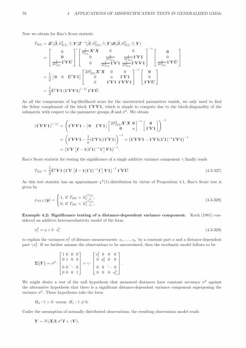
78 4 APPLICATIONS OF MISSPECIFICATION TESTS IN GENERALIZED GMMs
Now we obtain for Rao’s Score statistic
TRS = S ′(β, σ2ML, γ; Y )I−1(β, σ2
ML, γ; Y )S(β, σ2ML, γ; Y )
=
⎡⎢⎣ 00
12�σ4
ML1′V U
⎤⎥⎦′ ⎡⎢⎣
1�σ2
MLX ′X 0 00 n
2�σ4ML
12�σ4
ML1′V 1
0 12�σ4
ML1′V 1 1
2�σ4ML
1′V V 1
⎤⎥⎦−1 ⎡⎢⎣ 0
01
2�σ4ML
1′V U
⎤⎥⎦
=12[0 0 U ′V 1
]⎡⎣ 2σ2MLX ′X 0 0
0 n 1′V 10 1′V 1 1′V V 1
⎤⎦−1 ⎡⎣ 00
1′V U
⎤⎦=
12U ′V 1 (1′V V 1)(−1) 1′V U .
As all the components of log-likelihood score for the unrestricted parameters vanish, we only need to findthe Schur complement of the block 1′V V 1, which is simple to compute due to the block-diagonality of thesubmatrix with respect to the parameter groups β and σ2. We obtain
(1′V V 1)(−1) =
(1′V V 1− [0 1′V 1 ]
[2σ2
MLX ′X 00 n
]−1 [0
1′V 1
])−1
=(1′V V 1− 1
n(1′V 1)(1′V 1)
)−1
=(1′V V 1 − 1′V 1(1′1)−11′V 1
)−1
=(1′V
[I − 1(1′1)−11′]V 1
)−1.
Rao’s Score statistic for testing the significance of a single additive variance component γ finally reads
TRS =12U ′V 1
(1′V
[I − 1(1′1)−11′]V 1
)−11′V U . (4.3-327)
As this test statistic has an approximate χ2(1)-distribution by virtue of Proposition 4.1, Rao’s Score test isgiven by
φAV C(y) =
{1, if TRS > k
χ2(1)1−α ,
0, if TRS < kχ2(1)1−α ,
(4.3-328)
Example 4.2: Significance testing of a distance-dependent variance component. Koch (1981) con-sidered an additive heteroscedasticity model of the form
σ2i = a + b · s2
i (4.3-329)
to explain the variances σ2i of distance measurements s1, . . . , sn by a constant part a and a distance-dependent
part γs2i . If we further assume the observations to be uncorrelated, then the stochastic model follows to be
Σ{Y } = σ2 ·
⎡⎢⎢⎢⎣1 0 0 00 1 0 0
0 0. . . 0
0 0 0 1
⎤⎥⎥⎥⎦+ γ ·
⎡⎢⎢⎢⎣s21 0 0 00 s2
2 0 0
0 0. . . 0
0 0 0 s2n
⎤⎥⎥⎥⎦ .
We might desire a test of the null hypothesis that measured distances have constant accuracy σ2 againstthe alternative hypothesis that there is a significant distance-dependent variance component superposing thevariance σ2. These hypotheses take the form
H0 : γ = 0 versus H1 : γ �= 0.
Under the assumption of normally distributed observations, the resulting observation model reads
Y ∼ N(Xβ, σ2I + γV ).

4.4 Application 7: Testing for non-normality of the observation errors 79
4.4 Application 7: Testing for non-normality of the observation errors
Let us consider the linear functional model
Y = Xβ + U , (4.4-330)
where X ∈ Rn×m denotes a known design matrix of full rank and β ∈ R
m×1 a vector of unknown functionalparameters. We will assume for now that the errors U are uncorrelated and homoscedastic according to thestochastic model
Σ{U} = σ2I. (4.4-331)
We have used such a Gauss-Markov model, for instance, in Section 3 to obtain the UMPI statistic M for testinglinear restrictions Hβ = w. The exact χ2- or F -distribution of this test statistic has been derived from thebasic premise that the error variables are normally distributed. This normality assumption becomes even moreevident if we recall that we used the normal density/likelihood function to derive of the Likelihood Ratio andRao’s Score statistic for that problem. If the errors do not follow a normal distribution, then these tests arenot reliable anymore, because the exact distributions of these test statistics (and therefore the critical values)will be at least inaccurate, and the likelihood function will be misspecified.
Therefore, if we have serious doubts about the normality of the error variables, then we should test thisassumption. In this section, we will investigate a test of normality which fits into the framework of parametrictesting problems, and which may be derived conveniently on the basis of Rao’s Score statistic.
Let us start by recalling that the density of a univariate normal distribution is characterized by four param-eters: a variable mean µ, a variable variance σ2, a constant skewness γ1 = 0 (reflecting symmetry about themean), and a constant kurtosis γ2 = 0 (indicating a mesokurtic shape). The mean is then identical to the firstmoment
µ1 =∫ ∞
−∞xf(x)dx
and the variance identical to the second central moment
µ2 =∫ ∞
−∞(x − µ1)2f(x)dx,
whereas the skewness and kurtosis are based on the third and fourth central moments
µ3 =∫ ∞
−∞(x − µ1)3f(x)dx
and
µ4 =∫ ∞
−∞(x − µ1)4f(x)dx
through the relations
γ1 =µ3
µ3/22
(4.4-332)
and
γ2 =µ4
µ22
− 3 (4.4-333)
(see Stuart and Ord, 2003, p. 74 and 109). A natural idea is now to estimate the skewness and kurtosis fromthe given data and to compare these estimates with the values ascribed to the normal distribution. On theone hand, if the empirical skewness turns out to be significantly smaller/larger than 0, then the errors willhave a non-symmetrical distribution with a lower/upper tail that is heavier than for a normal distribution.On the other hand, if the empirical kurtosis is significantly smaller/larger than 0, then the errors will have aplatykurtic/leptokurtic distribution with a flatter/sharper top (see Stuart and Ord, 2003, p. 109). Unfortunately,it is not clear how large these deviations from 0 must be to indicate significant non-normality, because we donot know the probability distribution of the estimators for γ1 and γ2.

80 4 APPLICATIONS OF MISSPECIFICATION TESTS IN GENERALIZED GMMs
Nevertheless, this problem of testing H0 : γ1 = 0, γ2 = 0 versus H1 : γ1 �= 0, γ2 �= 0 may be tackled in aquite convenient way by considering Pearson’s collection of distributions WP . The density function ofeach univariate distribution within WP satisfies the differential equation
d
duln f(u; c0, c1, c2) =
c1 − u
c0 − c1u + c2u2(u ∈ R), (4.4-334)
where the parameters c0, c1, and c2 determine the shape of the density function f , and where u is a quantitymeasured about its mean, such as an error ui = yi − Xiβ in (4.4-330). We will see later that the densityfunction of the centered normal distribution (with µ = 0) satisfies (4.4-334) for c0 = σ2, c1 = 0, and c2 = 0.Furthermore, the parameters c1 and c2 correspond to the skewness and kurtosis through the relations
c1 =γ1(γ2 + 6)
õ2
10γ2 − 12γ21 + 12
(4.4-335)
and
c2 =3γ2
1 − 2γ2
10γ2 − 12γ21 + 12
(4.4-336)
(see Equation 6.4 in Stuart and Ord, 2003, p. 217), so that the problem of testing of H0 : γ1 = 0, γ2 = 0 versusH1 : γ1 �= 0, γ2 �= 0 is equivalent to testing H0 : c1 = 0, c2 = 0 versus H1 : c1 �= 0, c2 �= 0.
Let us now determine the general solution of (4.4-334). Integration of (4.4-334) yields
ln f(u; c0, c1, c2) + k =∫
c1 − u
c0 − c1u + c2u2du,
which we may rewrite as
ln f(u; c0, c1, c2) + k = g(u; c0, c1, c2) (k ∈ R),
where k denotes the integration constant and
g(u; c0, c1, c2) :=∫
c1 − u
c0 − c1u + c2u2du (4.4-337)
an antiderivative. Now, using exp(lnu) = u, the general solution of (4.4-334) follows to be
f(u; c0, c1, c2) = exp{g(u; c0, c1, c2) − k} = exp{−k} · exp{g(u; c0, c1, c2)} =: k∗ · exp{g(u; c0, c1, c2)}.(4.4-338)
The integration constant k∗ is determined by standardizing the area under f to 1, which yields
1 =
+∞∫−∞
f(u; c0, c1, c2)du =
+∞∫−∞
k∗ · exp g(u; c0, c1, c2)du = k∗ ·+∞∫
−∞exp g(u; c0, c1, c2)du.
Now, substituting k∗ = 1/∫ +∞−∞ exp g(u; c0, c1, c2) du into (4.4-338) leads to
f(u; c0, c1, c2) =exp g(u; c0, c1, c2)∫ +∞
−∞ exp g(u; c0, c1, c2) du(4.4-339)
as the standardized solution of (4.4-334).

4.4 Application 7: Testing for non-normality of the observation errors 81
Pearson’s collection of distributions comprises a large number of standard distributions and, as indicatedearlier, the normal distribution is its most prominent member. Some particularly useful members of WP aresummarized by the following proposition.
Proposition 4.2. The following univariate distributions are members of Pearson’s collection of distribution:
1. Centered normal distrubution N(0, σ2),
2. Gamma distribution G(b, p),
3. Beta distribution B(α, β),
4. Student distribution t(k).
Proof. 1. To see that the density function f(u; σ2) of N(0, σ2) satisfies (4.4-334), set c0 = σ2, c1 = c2 = 0 in(4.4-337), for which (4.4-339) becomes
f(u; σ2) =exp(∫ −u
σ2 du)∫ +∞
−∞ exp(∫ −u
σ2 du)du
=exp(
−u2
2σ2
)∫ +∞−∞ exp
(−u2
2σ2
)du
. (4.4-340)
The integral in the denominator is solved by using
+∞∫0
exp(−a2x2
)dx =
√π
2a(a > 0) (4.4-341)
(see Bronstein and Semendjajew, 1991, p. 66; Integral 3), where in the given case a2 = 1/2σ2 is positive as aconsequence of the fact that σ2 > 0 by definition. Also note that integration on (−∞, +∞) doubles the valueof (4.4-341) because of exp
(−a2(−x)2)
= exp(−a2x2
). Thus it follows that∫ +∞
−∞exp(−u2
2σ2du
)du =
√π ·
√2σ2, (4.4-342)
from which the density function
f(u; σ2) =1√2πσ
exp{−1
2
(u
σ
)2}
(4.4-343)
of the centered normal distribution is obtained.Proofs for 2.-4. are found, for instance, in Stuart and Ord (2003, Chap. 6).
Now, the log-likelihood function may be determined from the densities (4.4-339) with respect to the errorsui = yi − Xiβ (i = 1, . . . , n). If these error variables are assumed to be independently distributed, then thejoint density (as a function of y with additional parameters β) may be factorized as
f(y; β, c0, c1, c2) =n∏
i=1
exp g(ui; c0, c1, c2)∫ +∞−∞ exp g(ui; c0, c1, c2) dui
. (4.4-344)
Notice that the value of the integral in the denominator is only a function of c0, c1, and c2, not of β, because ui
acts there only as an integration variable. Defining the parameter vector as θ := [β′, c0, c1, c2]′, the log-likelihoodfunction follows to be
L(θ; y) = lnn∏
i=1
exp g(ui; c0, c1, c2)∫ +∞−∞ exp g(ui; c0, c1, c2) dui
=n∑
i=1
(g(ui; c0, c1, c2) − ln
∫ +∞
−∞exp g(ui; c0, c1, c2) dui
).

82 4 APPLICATIONS OF MISSPECIFICATION TESTS IN GENERALIZED GMMs
Taking the first partial derivatives with respect to the functional parameters βj (j = 1, . . . , m) yields
Sβj (θ; y) :=∂L(θ; y)
∂βj=
n∑i=1
∂g(ui; c0, c1, c2)∂βj
=n∑
i=1
∂
∂βj
∫c1 − ui
c0 − c1ui + c2u2i
dui
=n∑
i=1
∂ui
∂βj
∂
∂ui
∫c1 − ui
c0 − c1ui + c2u2i
dui = −n∑
i=1
Xi,jc1 − ui
c0 − c1ui + c2u2i
,
which defines the random variable
Sβj (θ; Y ) = −n∑
i=1
Xi,jc1 − Ui
c0 − c1Ui + c2U2i
. (4.4-345)
Peracchi (2001, p. 365) points out an elegant way to derive the score with respect to the parameters cj (j =0, . . . , 2), which shall be explained here in greater detail. Applying the partial derivative to both terms withinthe sum of the log-likelihood function gives
Scj (θ; y) :=∂L(θ; y)
∂cj=
n∑i=1
⎛⎝∂g(ui; c0, c1, c2)∂cj
− ∂
∂cjln
+∞∫−∞
exp g(ui; c0, c1, c2) dui
⎞⎠=
n∑i=1
⎛⎝∂g(ui; c0, c1, c2)∂cj
− 1∫ +∞−∞ exp g(ui; c0, c1, c2) dui
· ∂
∂cj
+∞∫−∞
exp g(ui; c0, c1, c2) dui
⎞⎠ .
Here we may interchange the integral and derivative, which results in
Scj (θ; y) =n∑
i=1
⎛⎝∂g(ui; c0, c1, c2)∂cj
− 1∫ +∞−∞ exp g(ui; c0, c1, c2) dui
·+∞∫
−∞
∂
∂cjexp g(ui; c0, c1, c2) dui
⎞⎠=
n∑i=1
⎛⎝∂g(ui; c0, c1, c2)∂cj
−∫ +∞−∞ exp g(ui; c0, c1, c2) · ∂g(ui;c0,c1,c2)
∂cjdui∫ +∞
−∞ exp g(ui; c0, c1, c2) dui
⎞⎠ .
The next step is to see that the integral in the denominator can be moved into the integral in the nominator,which allows us to apply (4.4-344), that is
Scj (θ; y) =n∑
i=1
⎛⎝∂g(ui; c0, c1, c2)∂cj
−+∞∫
−∞
exp g(ui; c0, c1, c2)∫ +∞−∞ exp g(ui; c0, c1, c2) dui
· ∂g(u; c0, c1, c2)∂cj
du
⎞⎠=
n∑i=1
⎛⎝∂g(ui; c0, c1, c2)∂cj
−+∞∫
−∞f(u; c0, c1, c2)
∂g(ui; c0, c1, c2)∂cj
dui
⎞⎠ .
Finally, we may use the fact that the integral represents the expectation of the random variable ∂g(Ui; c0, c1, c2)/∂cj ,which leads to the result
Scj (θ; Y ) =n∑
i=1
(∂g(Ui; c0, c1, c2)
∂cj− E
{∂g(Ui; c0, c1, c2)
∂cj
})(4.4-346)
as given in Peracchi (2001). To compute the partial derivatives ∂g(ui; c0, c1, c2)/∂cj regarding the antiderivativedefined in (4.4-337), we may again interchange the derivative and the integral. Then we obtain
∂g(ui; c0, c1, c2)∂c0
= −∫
c1 − ui
(c0 − c1ui + c2u2i )2
dui,
∂g(ui; c0, c1, c2)∂c1
=∫
1 · (c0 − c1ui + c2u2i ) − (c1 − ui)(−ui)
(c0 − c1ui + c2u2i )2
dui =∫
c0 + c2u2i − u2
i
(c0 − c1ui + c2u2i )2
dui,
∂g(ui; c0, c1, c2)∂c2
= −∫
(c1 − ui)u2i
(c0 − c1ui + c2u2i )2
dui.

4.4 Application 7: Testing for non-normality of the observation errors 83
Eventually, we will have to evaluate the scores at the ML estimates with the restrictions H0 : c1 = c2 = 0.Furthermore, the parameter c0 will be identical to the variance σ2 under these restrictions, as mentioned above.Then, evaluation of the partial derivatives at c1 = c2 = 0 with the parameters c0 = σ2 and β remainingunspecified gives
∂g(ui; σ2, 0, 0)∂c0
=∫
ui
σ4dui =
1σ4
∫ui dui =
u2i
2σ4,
∂g(ui; σ2, 0, 0)∂c1
=∫
σ2 − u2i
σ4dui =
1σ2
∫dui − 1
σ4
∫u2
i dui =ui
σ2− u3
i
3σ4,
∂g(ui; σ2, 0, 0)∂c2
=∫
u3i
σ4dui =
1σ4
∫u3
i dui =u4
i
4σ4.
These quantities define random variables whose expectations, under the restrictions H0, are given by
E
{∂g(ui; σ2, 0, 0)
∂c0
}=
E{U2i }
2σ4=
12σ2
,
E
{∂g(ui; σ2, 0, 0)
∂c1
}=
E{Ui}σ2
− E{U3i }
3σ4= 0,
E
{∂g(ui; σ2, 0, 0)
∂c2
}=
E{U4i }
4σ4=
34,
where we used the following facts about the moments of Ui: (1) E{Ui} = 0 by virtue of the first Markovcondition; (2) E{U2
i } = σ2 = µ2 in light of the second Markov condition; (3) c1 = γ1 = 0 implies E{U3i }µ3 = 0
because of (4.4-332); and (4) c2 = γ2 = 0 implies E{U4i } = µ4 = 3µ2
2 = 3σ4 due to (4.4-333). This gives finallythe components of the score (4.4-346)
Sσ2(θ; Y ) =n∑
i=1
(U2
i
2σ4− 1
2σ2
)=
12σ4
n∑i=1
U2i − n
2σ2, (4.4-347)
Sc1(θ; Y ) =n∑
i=1
(Ui
σ2− U3
i
3σ4− 0)
=1σ2
n∑i=1
Ui − 13σ4
n∑i=1
U3i (4.4-348)
Sc2(θ; Y ) =n∑
i=1
(U4
i
4σ4− 3
4
)=
14σ4
n∑i=1
U4i − 3n
4. (4.4-349)
To construct Rao’s Score statistic, the scores (4.4-345) and (4.4-347) - (4.4-349) must be evaluated at therestricted ML estimates θ. Under the restrictions c1 = c2 = c0, the Gauss-Markov model (4.4-330) and(4.4-331) has normally distributed errors U . Therefore, the restricted ML estimator for β is identical to theleast squares estimator β = (X ′X)−1X ′Y . The residuals are then estimated by U = Y − Xβ. This leads tothe restricted ML estimator for c0 = σ2, that is σ2
ML = U ′U/n, which differs from the least squares estimatoronly in using the factor 1/n instead of 1/(n − m). Finally, we will also use the estimators µj =
∑ni=1 U j
i /n
(j = 2, 3, 4) for the second, third, and fourth (central) moments (the first moment µj =∑n
i=1 Ui is zero as weassumed the presence of an intercept parameter).
Exploiting the orthogonality between the j-th column of X (i.e. the j-th row of X ′) and the vector ofestimated residuals, we obtain from (4.4-345)
Sβj (θ; Y ) = −n∑
i=1
Xi,j−Ui
σ4ML
=1
σ4ML
n∑i=1
Xi,jUi = 0, (4.4-350)
and from (4.4-347) - (4.4-349)
Sσ2(θ; Y ) =1
2σ4ML
n∑i=1
U2i − n
2σ2ML
=nσ2
ML
2σ4ML
− n
2σ2ML
= 0, (4.4-351)
Sc1(θ; Y ) =1
σ2ML
n∑i=1
Ui − 13σ4
ML
n∑i=1
U3i = − nµ3
3σ4ML
, (4.4-352)
Sc2(θ; Y ) =1
4σ4ML
n∑i=1
U4i − 3n
4=
nµ4
4σ4ML
− 3n
4. (4.4-353)

84 4 APPLICATIONS OF MISSPECIFICATION TESTS IN GENERALIZED GMMs
As already mentioned in Section 2.5.6, we see that the score vanishes in the direction of the unrestrictedparameters (β and σ2), because the estimates for the unrestricted parameters are given the freedom to satisfythe corresponding likelihood equations exactly, i.e. to maximize the log-likelihood function in those directions.
The derivation of the second partial derivatives of the log-likelihood function with respect to all the param-eters in θ, or equivalently of the first partial derivatives of the scores (4.4-345) and (4.4-347) - (4.4-349), is verylengthy. Therefore, we will refer to Proposition 2 in Bera and Jarque (1982), from which the information matrixat θ is obtained as
I(θ; Y ) =
⎡⎢⎢⎢⎢⎣1
�σ2ML
X ′X 0 0 00 n
2�σ4ML
0 3n2�σ2
ML
0 0 2n3�σ2
ML0
0 3n2�σ2
ML0 6n
⎤⎥⎥⎥⎥⎦ (4.4-354)
Now we obtain for Rao’s Score statistic
TRS = S ′(θ; Y )I−1(θ; Y )S(θ; Y )
=
⎡⎢⎢⎢⎣00
− n�µ33�σ4
MLn�µ4
4�σ4ML
− 3n4
⎤⎥⎥⎥⎦′ ⎡⎢⎢⎢⎢⎣
1�σ2
MLX ′X 0 0 00 n
2�σ4ML
0 3n2�σ2
ML
0 0 2n3�σ2
ML0
0 3n2�σ2
ML0 6n
⎤⎥⎥⎥⎥⎦−1 ⎡⎢⎢⎢⎣
00
− n�µ33�σ4
MLn�µ4
4�σ4ML
− 3n4
⎤⎥⎥⎥⎦If we define the subvectors
S1 :=[00
], S2 := n
[ − �µ33�σ4
ML�µ4
4�σ4ML
− 34
],
the submatrices
I11 :=
[1
�σ2ML
X ′X 00 n
2�σ4ML
], I12 = I ′
21 :=
[0 00 3n
2�σ2ML
], I22 :=
[2n
3�σ2ML
00 6n
],
and the Schur complements I(−1)11 , I(−1)
12 , I(−1)21 , I(−1)
22 as the blocks of the total inverse I−1(θ; Y ), then TRS
follows to be
TRS = S ′1I(−1)
11 S1 + S′2I(−1)
21 S1 + S ′1I(−1)
12 S2 + S ′2I(−1)
22 S2
= S ′2I(−1)
22 S2.
With
I(−1)22 = (I22 − I21I−1
11 I12)−1
=
⎛⎝[ 2n3�σ2
ML0
0 6n
]−[
0 00 3n
2�σ2ML
] [1
�σ2ML
X ′X 00 n
2�σ4ML
]−1 [0 00 3n
2�σ2ML
]⎞⎠−1
=
([2n
3�σ2ML
00 6n
]−[
0 00 3n
2�σ2ML
] [σ2
ML(X ′X)−1 00 2σ4
ML/n
] [0 00 3n
2�σ2ML
])−1
=
([2n
3�σ2ML
00 6n
]−[
0 00 9n
2
])−1
=1n
[32 σ2
ML 00 2
3
],
(which is a part of the result given in Proposition 3 by Bera and Jarque, 1982), we obtain
TRS = n
[ − �µ33�σ4
ML�µ4
4�σ4ML
− 34
]′ [32 σ2
ML 00 2
3
] [ − �µ33�σ4
ML�µ4
4�σ4ML
− 34
]= n
[ − �µ33�σ4
ML�µ4
4�σ4ML
− 34
]′ [ − �µ32�σ2
ML�µ4
6�σ4ML
− 12
]
= nµ2
3
6σ6ML
+ nµ2
4
24σ8ML
− nµ4
8σ4ML
− nµ4
8σ4ML
+ 3n/8
=n
6· µ2
3
σ6ML
+n
24
(µ2
4
σ8ML
− 6µ4
σ4ML
+ 9)
=n
6· µ2
3
σ6ML
+n
24
(µ4
σ4ML
− 3)2
.

4.4 Application 7: Testing for non-normality of the observation errors 85
Observe now that the definition of σ2ML is identical to that of the empirical second central moment µ2. Then,
if we define the empirical skewness
γ1 =µ3
µ3/22
, (4.4-355)
and the empirical kurtosis
γ2 =µ4
µ22
− 3, (4.4-356)
which depend on the estimated residuals of the Gauss-Markov model through the empirical moments µj =∑ni=1 U j
i (j = 2, . . . , 4), then Rao’s Score statistic takes its final form
TRS =n
6γ21 +
n
24γ22 . (4.4-357)
Evidently, this statistic measures the absolute deviations of the data’s skewness and kurtosis from the values 0,thus compares how far the distribution of the estimated residuals differs from a normal distribution. This testof normality is also called the Jarque-Bera test (Bera and Jarque, 1982).
Example 4.3: Testing the Gravity Dataset for non-normality. In Example 3.2 we considered a two-dimensional polynomial model of degree 1 with additional mean shift parameters. To check whether the errorsU in the model
Y = Xβ + Z∇ + U
follow a normal distribution, we first compute the residuals
u = y − Xβ − Z∇based on the least squares estimates[
β
∇
]=[
X ′X X ′ZZ ′X Z ′Z
]−1 [X ′yZ ′y
].
Contrary to Example 3.2, we use tildes instead of hats on top of the estimate ∇, because here the mean shiftparameters ∇, which were proven to be significant, naturally belong to the functional model. The tildes indicatethat the estimates have been determined under the restrictions c1 = c2 = 0. From these residuals we the obtainγ1 = −0.25 for the empirical skewness (4.4-355) and γ2 = −0.29 for the kurtosis measure (4.4-356). With thesevalues, Rao’s Score statistic (4.4-357) becomes TRS = 1.28, which is insignificant in light of the critical valuek
χ2(2)0.95 = 5.99. Therefore, we may assume the errors to be normally distributed, which is also roughly reflected
by the following histogram plot. �
−0.15 −0.1 −0.05 0 0.05 0.1 0.150
5
10
15
20
25
30
35
Figure 4.2. Histogram of the estimated residuals.

86 5 CONCLUSION AND OUTLOOK
5 Conclusion and Outlook
In the framework of the Gauss-Markov model with normally distributed errors, uniformly most powerful in-variant tests generally exist. These tests have three equivalent formulations: (1) the form obtained from adirect application of invariance principles, (2) the likelihood ratio test, and (3) Rao’s score test. Of the three,Rao’s score test is easiest to compute for problems where significance testing is required. If the testing probleminvolves unknown parameters within the weight matrix, or if the errors do not follow a normal distribution,then no uniformly most powerful invariant tests exist. In these cases too, Rao’s score test offers an attractivemethod that is both powerful and computationally convenient. This thesis has demonstrated that hypothesistesting by applying Rao’s score method is an effective - and in many cases optimal - approach for resolving awide range of problems faced in geodetic model analysis.
New satellite missions such as GOCE (Gravity Field and steady-state Ocean Circulation Explorer) requirepowerful and computationally feasible tests for diagnosing functional and stochastic models that are far morecomplex than the models considered in this thesis (cf. Lackner, 2006). To find convincing solutions to thesechallenges, it will be necessary for geodesists to further elaborate their understanding of statistical testing theory.Looking at the methodology currently offered by mathematical statistics, some directions of further researchare particularly promising. Rao’s score approach can be applied to a full range of testing problem fields suchas deformation analysis, time series analysis, or geostatistics - applications that have not yet been explored inmodern geodetic literature. It is crucial that geodesists develop a stronger expertise in the asymptotic behaviourof statistical theories, such as given in Lehmann and Romano (2005, Part II). This will be a necessary steptowards assessing the quality of geodetic hypothesis tests, such as those presented in Section 4, for which nostrict optimality criteria are applicable.
The scope of the theory presented in this thesis is restricted to a specific minimization problem regardingType I and Type II error probabilities within the class of invariant tests. However, minimizing error probabilitydoes not correspond to a minimization of costs when one considers losses in work time, computational time, oreven accuracy of estimated parameters. To overcome this limitation, hypothesis tests could be derived withinthe framework of decision theory, by minimizing a loss function which represents the expected loss/cost due toan erroneous test decision (cf. Lehmann and Romano, 2005, p. 59).
Finally, it is often argued that classical testing theory is too limited in that the test decision is always madeon the premise of a true null hypothesis, and that a priori information with respect to the unknown parametersmay not be used (see, for instance, Jaynes, 2003, Chapter 16). A theory which does allow the treatment ofthe null and the alternative hypothesis on equal grounds and incorporation of a priori information is offered byBayes statistics. Bayesian tests may be viewed as generalizations of likelihood ratio tests in that the likelihoodratio is extended by an a priori density with respect to the unknown parameters, which are treated as randomvariables (cf. Koch, 2000, Section 3.4). It would be highly instructive to formulate the model misspecificationtests developed in this thesis within the Bayesian framework and to compare them in terms of testing power,applicability to a wide range of problems, and computational convenience.

87
6 Appendix: Datasets
6.1 Dam Dataset
The numerical values of the observation model
y = Xβ + u, Σ{U} = σ2I,
for the Dam dataset used in Application 3 of Sect. 3.5 are given by⎡⎢⎢⎢⎢⎢⎢⎢⎢⎢⎢⎢⎢⎢⎢⎢⎢⎢⎢⎢⎢⎢⎢⎢⎢⎢⎢⎢⎢⎢⎢⎢⎢⎢⎢⎢⎢⎢⎢⎢⎢⎢⎢⎢⎢⎢⎢⎢⎢⎢⎢⎢⎢⎢⎢⎢⎢⎢⎢⎢⎢⎢⎢⎢⎢⎢⎣
3.43380.00180.00076.56876.56976.570−0.47777.04777.04667.70567.7061.444
66.26266.26266.2601.162
65.09765.098−0.002−0.00280.00079.99976.57076.56976.56977.04677.04767.70467.70666.26166.26166.26065.09865.099
⎤⎥⎥⎥⎥⎥⎥⎥⎥⎥⎥⎥⎥⎥⎥⎥⎥⎥⎥⎥⎥⎥⎥⎥⎥⎥⎥⎥⎥⎥⎥⎥⎥⎥⎥⎥⎥⎥⎥⎥⎥⎥⎥⎥⎥⎥⎥⎥⎥⎥⎥⎥⎥⎥⎥⎥⎥⎥⎥⎥⎥⎥⎥⎥⎥⎥⎦
=
⎡⎢⎢⎢⎢⎢⎢⎢⎢⎢⎢⎢⎢⎢⎢⎢⎢⎢⎢⎢⎢⎢⎢⎢⎢⎢⎢⎢⎢⎢⎢⎢⎢⎢⎢⎢⎢⎢⎢⎢⎢⎢⎢⎢⎢⎢⎢⎢⎢⎢⎢⎢⎢⎢⎢⎢⎢⎢⎢⎢⎢⎢⎢⎢⎢⎢⎣
+1 0 0 0 0 0 0 0 0 0 00 0 0 0 0 +1 0 0 0 0 00 0 0 0 0 0 +1 0 0 0 0
−1 0 0 0 0 +1 0 0 0 0 0−1 0 0 0 0 0 +1 0 0 0 0−1 0 0 0 0 0 0 +1 0 0 0−1 +1 0 0 0 0 0 0 0 0 0
0 −1 0 0 0 0 +1 0 0 0 00 −1 0 0 0 0 0 +1 0 0 00 0 −1 0 0 +1 0 0 0 0 00 0 −1 0 0 0 +1 0 0 0 00 0 −1 +1 0 0 0 0 0 0 00 0 0 −1 0 +1 0 0 0 0 00 0 0 −1 0 0 +1 0 0 0 00 0 0 −1 0 0 0 +1 0 0 00 0 0 −1 +1 0 0 0 0 0 00 0 0 0 −1 0 +1 0 0 0 00 0 0 0 −1 0 0 +1 0 0 00 0 0 0 0 −1 +1 0 0 0 00 0 0 0 0 0 −1 +1 0 0 00 0 0 0 0 0 0 0 +1 0 00 0 0 0 0 0 0 0 0 +1 0
−1 0 0 0 0 0 0 0 +1 0 0−1 0 0 0 0 0 0 0 0 +1 0−1 0 0 0 0 0 0 0 0 0 +1
0 −1 0 0 0 0 0 0 0 +1 00 −1 0 0 0 0 0 0 0 0 +10 0 −1 0 0 0 0 0 +1 0 00 0 −1 0 0 0 0 0 0 +1 00 0 0 −1 0 0 0 0 +1 0 00 0 0 −1 0 0 0 0 0 +1 00 0 0 −1 0 0 0 0 0 0 +10 0 0 0 −1 0 0 0 0 +1 00 0 0 0 −1 0 0 0 0 0 +1
⎤⎥⎥⎥⎥⎥⎥⎥⎥⎥⎥⎥⎥⎥⎥⎥⎥⎥⎥⎥⎥⎥⎥⎥⎥⎥⎥⎥⎥⎥⎥⎥⎥⎥⎥⎥⎥⎥⎥⎥⎥⎥⎥⎥⎥⎥⎥⎥⎥⎥⎥⎥⎥⎥⎥⎥⎥⎥⎥⎥⎥⎥⎥⎥⎥⎥⎦
⎡⎢⎢⎢⎢⎢⎢⎢⎢⎢⎢⎢⎢⎢⎢⎢⎢⎢⎣
H2
H3
H4
H5
H6
H7
H8
H9
H7′
H8′
H9′
⎤⎥⎥⎥⎥⎥⎥⎥⎥⎥⎥⎥⎥⎥⎥⎥⎥⎥⎦
+
⎡⎢⎢⎢⎢⎢⎢⎢⎢⎢⎢⎢⎢⎢⎢⎢⎢⎢⎢⎢⎢⎢⎢⎢⎢⎢⎢⎢⎢⎢⎢⎢⎢⎢⎢⎢⎢⎢⎢⎢⎢⎢⎢⎢⎢⎢⎢⎢⎢⎢⎢⎢⎢⎢⎢⎢⎢⎢⎢⎢⎢⎢⎢⎢⎢⎢⎣
u1
u2
u3
u4
u5
u6
u7
u8
u9
u10
u11
u12
u13
u14
u15
u16
u17
u18
u19
u20
u21
u22
u23
u24
u25
u26
u27
u28
u29
u30
u31
u32
u33
u34
⎤⎥⎥⎥⎥⎥⎥⎥⎥⎥⎥⎥⎥⎥⎥⎥⎥⎥⎥⎥⎥⎥⎥⎥⎥⎥⎥⎥⎥⎥⎥⎥⎥⎥⎥⎥⎥⎥⎥⎥⎥⎥⎥⎥⎥⎥⎥⎥⎥⎥⎥⎥⎥⎥⎥⎥⎥⎥⎥⎥⎥⎥⎥⎥⎥⎥⎦
(6.1-358)

88 6 APPENDIX: DATASETS
6.2 Gravity Dataset
Index Anomaly Latitude Longitude Index Anomaly Latitude Longitudei dg ◦ min ◦ min i dg ◦ min ◦ min1 15.11 48 10.26 16 19.01 47 14.91 46 41.99 13 40.002 15.13 48 13.97 16 20.24 48 15.03 46 37.09 13 50.043 14.80 48 18.72 16 25.85 49 15.01 46 39.45 14 18.824 15.02 48 43.15 16 18.20 50 15.07 46 33.27 14 02.635 15.11 48 30.75 16 37.30 51 15.03 47 46.26 12 56.566 15.25 48 41.56 16 52.24 52 15.09 47 36.09 12 42.247 15.02 48 21.72 15 24.23 53 15.07 47 16.94 12 29.008 15.07 48 11.88 14 31.68 54 15.06 47 17.75 12 46.079 15.07 48 07.54 14 52.73 55 15.09 47 25.13 13 13.15
10 14.91 48 09.56 15 06.06 56 15.01 47 08.05 13 40.8211 15.12 48 13.45 15 21.48 57 15.00 48 34.22 13 59.6912 15.09 48 10.32 15 37.15 58 15.09 48 15.41 13 02.3413 15.10 47 48.42 16 12.18 59 15.07 48 27.50 13 26.0714 15.06 47 39.61 15 53.51 60 15.10 48 18.52 14 14.8515 15.09 48 08.43 16 54.04 61 15.05 48 04.40 14 03.4316 15.04 47 45.98 16 27.31 62 14.99 47 31.66 11 42.4917 14.97 47 35.08 16 25.54 63 15.11 47 35.06 12 09.9818 15.04 47 42.41 16 54.87 64 15.00 47 29.02 10 43.3819 15.11 47 15.10 16 14.65 65 14.91 47 15.63 10 45.5620 15.15 47 24.82 16 29.78 66 14.95 47 18.51 11 04.5021 14.98 46 59.34 16 15.65 67 14.95 47 16.83 10 59.0022 15.10 47 53.35 16 39.69 68 15.05 47 16.07 11 16.2423 15.03 47 44.49 15 18.64 69 14.91 47 25.52 11 13.9024 14.93 47 36.95 15 46.11 70 14.94 47 25.76 11 14.8125 15.10 47 23.54 13 41.47 71 15.08 47 23.78 11 49.3526 15.20 47 23.16 15 05.63 72 15.06 47 29.19 12 03.9627 15.09 47 24.93 16 01.25 73 14.98 47 07.76 10 15.9328 14.98 47 04.68 13 55.63 74 14.93 47 08.95 10 34.7029 15.07 47 02.35 15 10.19 75 14.89 47 08.05 10 30.9930 15.13 47 03.41 15 25.04 76 14.92 47 14.22 10 44.3331 15.12 47 01.59 15 29.14 77 14.92 47 10.92 10 37.0332 15.16 47 04.59 15 34.97 78 15.13 47 11.84 10 39.4133 15.11 47 04.19 15 44.22 79 14.90 47 13.30 10 45.3534 15.13 46 53.11 15 29.91 80 14.92 47 14.08 10 51.2435 15.06 47 40.55 15 29.64 81 15.06 47 03.85 11 29.2836 15.01 47 36.45 15 40.38 82 15.03 47 07.63 11 27.1737 15.11 47 04.77 15 59.64 83 15.03 47 13.92 11 23.1738 14.93 47 00.05 12 32.54 84 15.05 47 14.04 11 52.8739 14.90 46 56.21 12 34.42 85 14.85 46 58.09 10 32.1240 15.00 46 49.03 12 47.28 86 14.82 46 50.92 10 30.3341 15.01 46 49.70 12 45.45 87 14.69 47 21.65 10 49.8742 14.82 46 54.75 13 15.50 88 14.89 47 31.80 9 51.8043 15.04 46 50.30 13 22.21 89 15.13 47 27.44 9 38.4444 14.92 46 48.97 13 25.04 90 14.98 47 25.84 9 45.3845 14.83 46 49.89 14 26.78 91 14.95 47 07.95 10 07.3146 15.11 46 39.85 12 59.82

89
References
Arnold, S.F. (1981). The theory of linear models and multivariate analysis. Wiley, New York.
Arnold, S.F. (1985). Sufficiency and invariance. Statistics & Probability Letters 3: 275-279.
Arnold, S.F. (1990). Mathematical statistics. Prentice Hall, Englewood Cliffs, New Jersey.
Baarda, W. (1967). Statistical concepts in geodesy. Publications on Geodesy (New Series), Vol. 1, Number 4,Netherlands Geodetic Commission, Delft.
Baarda, W. (1968). A testing procedure for use in geodetic networks. Publications on Geodesy (New Series),Vol. 2, Number 5, Netherlands Geodetic Commission, Delft.
Bera, A.K. and C.M. Jarque (1982). Model specification tests. A simultaneous approach. Journal of Economet-rics, 20:59-82.
Birkes, D. (1990). Generalized likelihood ratio tests and uniformly most powerful tests. The American Statisti-cian, 44(2):163-166.
Bronstein, I.N. and K.A. Semendjajew (1991). Taschenbuch der Mathematik. Teubner, Stuttgart.
Casella, G. and R.L. Berger (2002). Statistical inference. Second edition. Duxbury, Pacific Grove, California.
Cox, D.R. and D.V. Hinkley (1974). Theoretical statistics. Chapman and Hall, London.
Dudewicz, E.J. and S. Mishra (1988). Modern mathematical statistics. Wiley, New York.
Engle, R.F. (1984). Wald, likelihood ratio, and Lagrange multiplier tests in econometrics. Z. Griliches and M.D.Intriligator (eds.): Handbook of Econometrics, Vol. 2:775-826.
Godfrey, L.G. (1988). Misspecification tests in econometrics. Cambridge University Press, Cambridge.
Hamilton, J.D. (1994). Time series analysis. Princeton University Press, Princeton.
Jaeger, R. et al. (2005). Klassische und robuste Ausgleichungsverfahren. Wichmann, Heidelberg.
Jaynes, E.T. (2003). Probability theory. The logic of science. Cambridge University Press, Cambridge.
Johnson, N.L. and S. Kotz (1970). Distributions in statistics: continuous univariate distributions, Vol. 1. Wiley,New York.
Johnson, N.L. and S. Kotz (1970). Distributions in statistics: continuous univariate distributions, Vol. 2. Wiley,New York.
Koch, K.-R. (1981). Varianz- und Kovarianzkomponentenschatzung fur Streckenmessungen auf Eichlinien. All-gemeine Vermessungs-Nachrichten, 88:125-132.
Koch, K.-R. (1999). Parameter estimation and hypothesis testing in linear models. Springer, Heidelberg.
Koch, K.-R. (2000). Einfuhrung in die Bayes-Statistik. Springer, Heidelberg.
Kramer, W. and H. Sonnberger (1986). The linear regression model under test. Physica, Heidelberg.
Kreyszig, E. (1998). Statistische Methoden und ihre Anwendungen. Vandenhoeck and Ruprecht, Gottingen.
Lackner, B. (2006). Datainspection and hypothesis tests of very long time series applied to GOCE satellite
gravity gradiometry data. Dissertation, Graz University of Technology.
Lehmann, E.L. (1959a). Testing statistical hypotheses. First edition. Wiley, New York.
Lehmann, E.L. (1959b). Optimum invariant tests. Annals of Mathematical Statistics, 30:881-884.
Lehmann, E.L. and J.P. Romano (2005). Testing statistical hypotheses. Third edition. Springer, New York.
Meissl, P. (1982). Least squares adjustment - a modern approach. Mitteilungen der geodatischen Institute derTechnischen Universitat Graz, Vol. 43.

90
Meyer, C.D. (2000). Matrix analysis and applied linear algebra. SIAM.
Neyman, J. and E.S. Pearson (1928). On the use and interpretation of certain test criteria for purposes of
statistical inference. Biometrika, 20A:175-240,263-295.
Neyman, J. and E.S. Pearson (1933). On the problem of the most efficient tests of statistical hypotheses.
Philosophical Transactions of the Royal Society of London, Series A, 231:289-337.
Olive, D.J. (2006). A course in statistical theory. Online document, Department of Mathematics, SouthernIllinois University. www.math.siu.edu/olive/infbook.htm.
Peracchi, F. (2001). Econometrics. Wiley, New York.
Pope, A.J. (1976). The statistics of residuals and the detection of outliers. NOAA Technical Report NOS65NGS1, US Department of Commerce, National Geodetic Survey, Rockville, Maryland.
Rao, C.R. (1948). Large sample tests of statistical hypotheses concerning several parameters with applications
to problems of estimation. Proceedings of Cambridge Philosophical Society, 44:50-57.
Rao, C.R. (1973). Linear statistical inference and its applications. Wiley, New York.
Rousseeuw, P.J. and A.M. Leroy (2003). Robust regression and outlier detection. Wiley, New York.
Schuh, W.D. (1996). Tailored numerical strategies for the global determination of the Earth’s gravity field.Mitteilungen der geodatischen Institute der Technischen Universitat Graz, Vol. 81.
Schuh, W.-D. (2006). Ausgleichungsrechnung und Statistik III. Lecture notes, Institute of Geodesy and Geoin-formation, University of Bonn.
Schuh, W.-D. (2006). Seminar Robuste Parameterschatzung. Lecture notes, Institute of Geodesy and Geoinfor-mation, University of Bonn.
Silvey, S.D. (1959). The Lagrangian multiplier test. Annals of Mathematical Statistics, 30:389-407.
Stuart, A., Ord, J.K., and S. Arnold (1999). The advanced theory of statistics, Vol. 2A: Classical inference and
the linear model. Arnold, London.
Stuart, A. and J.K. Ord (2003). The advanced theory of statistics, Vol. 1: Distribution theory. Arnold, London.
Teunissen, P.J.G. (2000). Testing theory. Delft University Press, Delft.

Acknowledgment
This thesis is the result of my studies in the field of adjustment theory and statistics at the Institute of Geodesyand Geoinformation at the University of Bonn. This opportunity was granted to me by Prof. Dr. techn. W.-D. Schuh, whose supervision was the perfect mix of non-restrictive guidance and open-minded dialogue. I amdeeply indebted to him for the time and energy he invested into supporting and discussing my ideas. I also wantto thank Prof. Dr. rer. nat. H.-P. Helfrich for serving as second referee. Further, I acknowledge the support bythe BMBF Geotechnologien programmes (Grants 03F0329C and 03F0421B).
My very special thanks goes to Jeramy Flora. Without her love, patience, and ideas throughout the years,this thesis (and my own nervous system) would not exist.