on the robustness and efficiency of integration algorithms for a 3d

INTERNATIONAL JOURNAL FOR NUMERICAL METHODS IN ENGINEERINGInt. J. Numer. Meth. Engng (2010)Published online in Wiley InterScience (www.interscience.wiley.com). DOI: 10.1002/nme.2964

On the robustness and efficiency of integration algorithms for a 3Dfinite strain phenomenological SMA constitutive model

J. Arghavani1,∗,†, F. Auricchio2,3,4, R. Naghdabadi1,5 and A. Reali2,4

1Department of Mechanical Engineering, Sharif University of Technology, 11155-9567 Tehran, Iran2Dipartimento di Meccanica Strutturale, Università degli Studi di Pavia, Italy

3Center for Advanced Numerical Simulation (CeSNA), IUSS, Pavia, Italy4European Centre for Training and Research in Earthquake Engineering (EUCENTRE), Pavia, Italy

5Institute for Nano-Science and Technology, Sharif University of Technology, 11155-9567 Tehran, Iran

SUMMARY

Most devices based on shape memory alloys experience large rotations and moderate or finite strains.This motivates the development of finite-strain constitutive models together with the appropriate compu-tational counterparts. To this end, in the present paper a three-dimensional finite-strain phenomenologicalconstitutive model is investigated and a robust and efficient integration algorithm is proposed. Properlydefining the variables, extensively used regularization schemes are avoided and a nucleation–completioncriterion is defined. Moreover, introducing a logarithmic mapping, a new form of time-discrete equationsis proposed. The solution algorithm as well as a suitable initial guess for the resultant nonlinear equationsare also deeply discussed. Extensive numerical tests are performed to show robustness as well as efficiencyof the proposed integration algorithm. Implementation of the integration algorithm within a user-definedsubroutine UMAT in the commercial nonlinear finite element software ABAQUS/Standard makes alsopossible the solution of a variety of boundary value problems. The obtained results show the efficiencyand robustness of the proposed approach and confirm the improved efficiency (in terms of solution CPUtime) when a nucleation–completion criterion is used instead of regularization schemes, as well as whena logarithmic mapping is used for the time-discrete evolution equation instead of an exponential mapping.Copyright � 2010 John Wiley & Sons, Ltd.

Received 20 January 2010; Revised 15 April 2010; Accepted 25 May 2010

KEY WORDS: shape memory alloys; finite strain; solution algorithm; logarithmic mapping; exponentialmapping; UMAT

∗Correspondence to: J. Arghavani, Department of Mechanical Engineering, Sharif University of Technology, 11155-9567 Tehran, Iran.

†E-mail: [email protected]

Copyright � 2010 John Wiley & Sons, Ltd.

J. ARGHAVANI ET AL.

1. INTRODUCTION

Shape memory alloys (SMA) are well-known materials exhibiting special properties, known assuper-elasticity or pseudo-elasticity (PE), one-way and two-way shape memory effects (SME)[1, 2], suitable for industrial applications. For example, nowadays, pseudo-elastic Nitinol is acommon and a well-known engineering material in the medical industry [3, 4].

The origin of SMA features is a reversible thermo-elastic martensitic phase transformationbetween a high symmetry, austenitic phase and a low symmetry, martensitic phase. Austenite isa solid phase, usually characterized by a body-centered cubic crystallographic structure, whichtransforms into martensite by means of a lattice shearing mechanism. When the transformationis driven by a temperature decrease, martensite variants compensate each other, resulting in nomacroscopic deformation. However, when the transformation is driven by the application of a load,specific martensite variants, favorable to the applied stress, are preferentially formed, exhibitinga macroscopic shape change in the direction of the applied stress. Upon unloading or heating,this shape change disappears through the reversible conversion of the martensite variants into theparent phase [1, 5].

For a stress-free SMA material, four characteristic temperatures can be identified as the startingand finishing temperatures during forward transformation (austenite to martensite), Ms and M f ,as well as the starting and finishing temperatures during reverse transformation, As and A f .Accordingly, in a stress-free condition, at a temperature above A f , only the austenitic phase isstable, while at a temperature below M f , only the martensitic phase is stable. On the other hand,by applying a stress at a temperature above A f SMAs exhibit pseudo-elastic behavior with a fullrecovery of inelastic strain upon unloading, while at a temperature below Ms , the material presentsthe shape memory effect with permanent inelastic strains upon unloading which may be recoveredby heating.

In most applications, SMAs experience general thermo-mechanical loads, which are morecomplicated than uniaxial or multiaxial proportional loadings, typically undergoing very largerotations and moderate strains (i.e. in the range of 10% for polycrystals [1]). For example, withreference to biomedical applications, stent structures are usually designed to significantly reducetheir diameter during the insertion into a catheter; thereby, large rotations combined with moderatestrains occur and the use of a finite deformation scheme is preferred.

The majority of the current 3D macroscopic constitutive models of SMAs has been developedin the small deformation regime. Among different constitutive models, the phenomenologicalones developed within the continuum thermodynamics with internal variables framework are ofmost engineering interest. For example, Raniecki and Lexcellent [6, 7] have developed the so-called RL models that are able to incorporate the basic features of SMA behavior. Based on aRL model, Panico and Brinson [8] decompose the inelastic strain into a transformation and areorientation part to consider martensite reorientation in their proposed constitutive model. Whileall of the above mentioned models use two limit functions to describe forward and reverse-phasetransitions, some models [9, 10] use only one limit function for both the forward and reversetransformations, simplifying considerably the numerical implementation. Helm and Haupt [10]have developed a thermo-mechanically coupled model to represent the main effects of materialbehavior under multiaxial loadings, comparing with the experimental data by Helm [11]. Recently,Arghavani et al. [12] have introduced a new set of internal variables including a scalar and atensor describing, respectively, pure phase transformation and pure reorientation and proposed aconstitutive model to improve the description of SMA behavior under the multiaxial loadings.

Copyright � 2010 John Wiley & Sons, Ltd. Int. J. Numer. Meth. Engng (2010)DOI: 10.1002/nme

ROBUSTNESS AND EFFICIENCY OF INTEGRATION ALGORITHMS FOR AN SMA

Numerical implementation of SMA models in the small-strain regime has also been studied inseveral works [13–17]. Asymmetry in tension and compression [16, 18], transformation surfaces[19], transformation-induced plasticity [20, 21], reorientation and detwinning [22, 23] and thermo-mechanical coupling [10, 24] are some of other aspects of SMA behavior studied by researchersin the small-strain regime.

Finite deformation SMA constitutive models available in the literature have been mainly devel-oped by extending small-strain constitutive models. The approach in most cases is based on themultiplicative decomposition of the deformation gradient into an elastic and an inelastic or transfor-mation part [25–34], although there are some models which have utilized an additive decompositionof the strain rate tensor into an elastic and an inelastic part [35]. In the following, we mentionsome of the finite deformation SMA constitutive models currently available in the iterature.

The model by Auricchio and Taylor [25] is apparently the first macroscopic SMA constitutivemodel taking into account finite deformation PE. Disregarding the first invariant of stress, thismodel reduces to Raniecki and Lexcellent model (RL model) [6] when linearized. Pethö [27]decomposes the total deformation gradient into elastic, plastic, and phase transformation parts,describing elasticity using an integrable hypoelastic model based on the logarithmic rate. Ziolkowski[28] extends a version of the RL model [6, 7] to the large deformation regime, considering thermo-mechanical coupling effects. Helm [11, 29] uses a double multiplicative decomposition of thedeformation gradient‡ and presents a finite strain model in the framework of thermoviscoplasticity.Similar to Helm and Haupt [10], Reese and Christ [30] use a double multiplicative decompositionof the deformation gradient and propose a pseudo-elastic finite strain model. They also suggesta new kind of exponential map where the exponential function is suitably computed by meansof the spectral decomposition. In another work, Christ and Reese [31] include also the thermo-mechanical coupling effects, shape memory effect and asymmetry in tension and compressionin [30] and simulate several boundary value problems. Based on a multiplicative decomposition,Evangelista et al. [32] extend the small-strain model proposed by Souza et al. [9] into finite strainregime. Recently, Thamburaja [33] has developed a finite-deformation-based, thermo-mechanicallycoupled and non-local phenomenological SMA model which is able to determine the positionand motion of austenite–martensite interfaces during the phase transformations. More recently,Arghavani et al. [34] have used a multiplicative decomposition of the deformation gradient intoelastic and inelastic parts together with an additive decomposition of the inelastic strain rate tensorinto transformation and reorientation parts to extended the small-strain model proposed by Panicoand Brinson [8] into finite strain regime.

While all the above-mentioned references use a multiplicative decomposition of the deformationgradient, Müller and Bruhns [35] utilize an additive decomposition of the strain rate tensor intoan elastic and a phase transformation part. In particular, they extend the RL small-strain model[7] to take into account finite deformations and finally reach a rate constitutive model in terms ofthe logarithmic spin tensor. Moreover, some large strain non-phenomenological models have beenproposed in the literature (see e.g. [36–39]).

In the present work, we focus on a finite-strain extension of the small-strain constitutive modelinitially proposed by Souza et al. [9] and extensively studied in references [13–15]. The final

‡The deformation gradient is multiplicatively decomposed into three parts; besides the elastic deformation gradient,the second part represents the deformation during the phase transformation and the third, the so-called dissipativedeformation gradient, correlates with the energy dissipation.


J. ARGHAVANI ET AL.

format of the obtained equations coincides with the one proposed by Evangelista et al. [32] butwe wish to remark that the approach followed herein in the derivation has some non-negligibledifferences as discussed later on. Moreover, to make this work self-contained, we present detailsof constitutive model development which can also be found in e.g. [29–32]. However, the paperemphasis is clearly on numerical aspect associated to the presented finite-strain model and thediscussion is organized as follows.

In Section 2, based on a multiplicative decomposition of the deformation gradient into elastic andtransformation parts, we present the time-continuous finite-strain constitutive model. In Section 3,based on an exponential mapping, a time-discrete scheme is investigated. We then introduce alogarithmic mapping and use it to propose an alternative form of the time-discrete equations.Moreover, we introduce a nucleation–completion condition and discuss appropriate initial guessesfor the Newton–Raphson method used in the solution procedure. Section 4 presents uniaxialas well as multiaxial non-proportional tests to check the numerical algorithm robustness andefficiency. We also compare the convergence behavior of different solution schemes as well asdifferent time-discrete forms of the evolution equation. In Section 5, by implementing the proposedintegration algorithm within a user-defined subroutine (UMAT) in the commercial nonlinear finiteelement software ABAQUS/Standard and considering both pseudo-elastic and shape memory effectbehaviors, we simulate the extension of a spring and the crimping of a medical stent, comparingthe solution CPU time for different approaches. We finally draw conclusions in Section 6.

2. A 3D FINITE-STRAIN SMA CONSTITUTIVE MODEL: TIME-CONTINUOUS FRAME

We use a multiplicative decomposition of the deformation gradient and present a thermodynamicallyconsistent finite-strain constitutive model as it has already been done e.g. by Helm [29], Reeseand Christ [30, 31], Evangelista et al. [32] and recently, by Arghavani et al. [34]. The finite-strainconstitutive model takes its origin from the small-strain constitutive model proposed by Souzaet al. [9] and improved and discussed by Auricchio and Petrini [13–15].

2.1. Constitutive model development

Considering a deformable body, we denote with F the deformation gradient and with J its deter-minant, supposed to be positive. The tensor F can be uniquely decomposed as:

F=RU=VR (1)

where U and V are the right and left stretch tensors, respectively, both positive definite andsymmetric, while R is a proper orthogonal rotation tensor. The right and left Cauchy–Greendeformation tensors are then respectively defined as:

C=FTF, b=FFT (2)

and the Green–Lagrange strain tensor, E, reads as:

E= C−12

(3)

where 1 is the second-order identity tensor. Moreover, the velocity gradient tensor l is given as:

l= FF−1 (4)



The symmetric and anti-symmetric parts of l supply the strain rate tensor d and the vorticitytensor w, i.e.:

d= 12 (l+ lT), w= 1

2 (l− lT) (5)

Taking the time derivative of Equation (3) and using (4) and (5), it can be shown that:

E=FTdF (6)

Following a well-established approach adopted in plasticity [40, 41] and already used for SMAs[11, 25–32, 34], we assume a local multiplicative decomposition of the deformation gradient intoan elastic part Fe, defined with respect to an intermediate configuration, and a transformationone Ft , defined with respect to the reference configuration. Accordingly:

F=FeFt (7)

As experimental evidences indicate that the transformation flow is nearly isochoric, we imposedet(Ft )=1, which after taking the time derivative results in:

tr(dt )=0 (8)

We define Ce=FeTFe and Ct =FtTFt as the elastic and the transformation right Cauchy–Greendeformation tensors, respectively, and using definition (2) and (7), we obtain:

Ce=Ft−TCFt−1 (9)

To satisfy the principle of material objectivity, the Helmholtz free energy has to depend on Fe

only through the elastic right Cauchy–Green deformation tensor; it is moreover assumed to be afunction of the transformation right Cauchy–Green deformation tensor and of the temperature, T ,in the following form:

�=�(Ce,Ct ,T )=�e(Ce)+�t (Et ,T ) (10)

where �e(Ce) is a hyperelastic strain energy function and Et = (Ct −1)/2 is the transformationstrain. We remark that in proposing decomposition (10), we have assumed the same materialbehavior for the austenite and martensite phases. In addition, we assume �e(Ce) to be an isotropicfunction of Ce; it can be therefore expressed as:

�e(Ce)=�e(ICe , IICe , IIICe ) (11)

where ICe , IICe , IIICe are the invariants of Ce. We also define �t in the following form[9, 13–15, 32]:

�t (Et ,T )=�M (T )‖Et‖+ 12h‖Et‖2+IεL (‖Et‖) (12)

where �M (T )=�〈T −T0〉 and �, T0 and h are material parameters; the Macaulay bracket calculatesthe positive part of the argument, i.e. 〈x〉= (x+|x |)/2, and the norm operator is defined as ‖A‖=√A :AT, with A :B= AijBij.Moreover, in Equation (12) we also use the indicator function IεL defined as:

IεL (‖Et‖)={0 if ‖Et‖�εL

+∞ otherwise(13)


J. ARGHAVANI ET AL.

to satisfy the constraint on the transformation strain norm (i.e. ‖Et‖�εL ). The material parameterεL is the maximum transformation strain norm in a uniaxial test.

Taking the time derivative of Equation (9) and using (4), the material time derivative of theelastic right Cauchy–Green deformation tensor is obtained as:

Ce=−ltTCe+Ft−TCFt−1−Celt (14)

We now use Clausius–Duhem inequality form of the second law of thermodynamics:

S : 12 C−(�+�T )�0 (15)

where S is the second Piola–Kirchhoff stress tensor related to the Cauchy stress a through:

S= JF−1aF−T (16)

and � is the entropy. Substituting (10) into (15), we obtain:

S :1

2C−

(��e

�Ce: Ce+ ��t

�Et: Et + ��t

�TT

)−�T�0 (17)

Now, substituting (14) into (17), after some mathematical manipulations, we obtain:(S−2Ft−1 ��e

�CeFt−T

):1

2C+2Ce ��e

�Ce: lt −X : Et−

(�+ ��t

�T

)T�0 (18)

where

X=hEt+(�M (T )+�)N (19)

and

N= Et

‖Et‖ (20)

The positive variable � results from the indicator function subdifferential �IεL (‖Et‖) and it issuch that: {

��0 if ‖Et‖=εL

�=0 otherwise(21)

In deriving (18), we have used the isotropic property of �e(Ce), implying that Ce and ��e/�Ce

are coaxial. Following standard arguments, we finally conclude:

S=2Ft−1 ��e

�CeFt−T

�=−��t

�T,

(22)

Using a classical property of second-order tensor double contraction, i.e. A : (BC)=B : (ACT)=C :(BTA), we conclude:

X : Et = (FtXFtT) :dt (23)



In deriving (23), we have used the following relation:

Et =FtTdtFt (24)

Substituting (22) and (23) into (18) and taking advantage of the symmetry of Ce(��e/�Ce), thedissipation inequality can be written as:

(P−K) :dt�0 (25)

where

P = 2Ce ��e

�Ce

K = FtXFtT(26)

To satisfy the second law of thermodynamics, (25), we define the following evolution equation:

dt = �(P−K)D

‖(P−K)D‖ (27)

where we denote with a superscript D the deviatoric part of a tensor. Moreover, we highlight that(27) satisfies the inelastic deformation incompressibility condition (8).

To describe the phase transformation, we choose the following limit function:

f =‖(P−K)D‖−R (28)

where the material parameter R is the elastic region radius. Similarly to plasticity, we also introducethe consistency parameter and the limit function satisfying the Kuhn–Tucker conditions:

f �0, ��0, � f =0 (29)

In conclusion, the constitutive model in the finite deformation regime can be finally summarizedas follows:

• Stress quantities:

S= 2Ft−1 ��e

�CeFt−T

P= 2Ce ��e

�Ce

X= hEt +(�M +�)N

K= FtXFtT

• Evolution equation:

dt = �(P−K)D

‖(P−K)D‖


J. ARGHAVANI ET AL.

• Limit function:

f =‖(P−K)D‖−R

• Kuhn–Tucker conditions:

f�0, ��0, � f =0

2.2. Representation with respect to the reference configuration

In the previous section, using a multiplicative decomposition of the deformation gradient intoelastic and transformation parts, we derived a finite-strain constitutive model. However, while Fand Ft are defined with respect to the reference configuration, Fe is defined with respect to anintermediate configuration. Following Reese and Christ [30] and Vladimirov et al. [42], we recastall equations in terms of C (control variable) and Ct (internal variable) which are described withrespect to the reference configuration, allowing to express all equations in a Lagrangian form,which also apparently confirms the constitutive model objectivity.

As a hyperelastic strain energy function �e has been introduced in terms of Ce (i.e. with respectto the intermediate configuration), we first investigate it.

As introduced in (11), �e depends on Ce only through its invariants, which are equal to theinvariants of CCt−1. In fact, for the first invariant the following identity holds:

ICe = tr(Ce)= tr(Ft−TCFt−1)= tr(CFt−1Ft−T)= tr(CCt−1)= ICCt−1 (30)

and similar relations hold for the second and the third invariants.Accordingly, we may write:

��e

�Ce=�11+�2Ce+�3Ce2 (31)

where �i =�i (ICCtr−1, IICCt−1, IIICCt−1). Substituting (31) into (22)1 and using (9), we concludethat:

S=2(�1Ct−1+�2Ct−1CCt−1+�3Ct−1(CCt−1)2) (32)

which expresses the second Piola–Kirchhoff stress tensor in terms of quantities computed withrespect to the reference configuration.

In order to find the Lagrangian form of the evolution equation, we substitute (27) into (24) andobtain:

Et = �FtT (P−K)D

‖(P−K)D‖Ft (33)

or equivalently,

Ct =2�FtT (P−K)D

‖(P−K)D‖Ft (34)

Focusing on the first term in the right-hand side of Equation (34), we may observe that:

FtTPFt = (FtCeFt )

(2Ft−1 ��e

�CeFt−T

)Ct =CSCt (35)



while, focusing on the second term in the right-hand side of equation (34), we may observe that:

FtTKFt =FtTFtXFtTFt =CtXCt (36)

We may then conclude:

FtT(P−K)Ft =YCt (37)

and obtain from (35)–(37):

Y=CS−CtX (38)

Moreover, we have:

FtT(P−K)DFt = FtT(P−K− 13 tr(P−K)1)Ft

= (CSCt −CtXCt − 13 tr(CS)C

t + 13 tr(C

tX)Ct )=YDCt (39)

yielding

(P−K)D =Ft−TYDFtT (40)

and

‖(P−K)D‖=‖YD‖ (41)

Now, we substitute (40) and (41) into (28) and (33) to obtain:

f =‖YD‖−R (42)

and

Ct =2�YD

‖YD‖Ct = �A= �A1Ct (43)

where A=2YD/‖YD‖Ct and A1=2YD/‖YD‖.

2.3. Presenting a singularity-free and continuous definition for N

We note that, according to (20), the variableN is not defined for the case of vanishing transformationstrain. Despite some discussions in the paper by Auricchio and Petrini [13],§ regularization schemeshave extensively been used in the literature to overcome this problem. For example Helm andHaupt [10] propose the following regularization scheme also used in [8, 21, 30, 31, 43]:

‖Et‖=√

‖Et‖2+ (44)

§Auricchio and Petrini [13] tried to define a non-singular equation in the small-strain regime. However, the approachis completely different from the one followed herein which is based on a well-defined N. In fact, in [13] anon-singular variable corresponding to limit function f (or, equivalently, the linearized form of ‖Y‖) is presented.


J. ARGHAVANI ET AL.

where is a user-defined parameter (typical value: 10−7). In Auricchio and Petrini [14] and adoptedalso in [15, 32], another proposed regularization scheme is as follows:

‖Et‖=‖Et‖− dd+1d

d−1(‖Et‖+d)

d−1d (45)

where d is again a user-defined parameter (typical value: 0.02). Regularization schemes (44) and(45) are indeed equivalent, despite they have different forms.

While using a regularization scheme has some advantages in removing singularity in N andin giving a smooth transition from austenitic to martensitic phase and vice versa with a quitesimple approach, it has however the disadvantage of transforming a large part of the elastic regioninto a region of nonlinear material response.¶ This significantly increases the solution time andconsequently decreases the numerical efficiency, especially for boundary value problems in whichconsiderable part of the structure remains elastic (e.g. a stent structure). In the following, motivatedby the work by Arghavani et al. [12] in the small-strain regime, we suggest to avoid a regularizedform for ‖Et‖ and to deal with the case of vanishing transformation strain through a carefulanalytical study of the limiting conditions. We start investigating a condition in which Et starts

to evolve from a zero value (indicated in the following as Nucleation), i.e. Et =0 with ˙‖Et‖>0.Substituting Ct =1 into (38) (also see (19) and (32)) we conclude that YD = (CSe)D . We nowconsider (43) which yields:

Et = 1

2Ct = �

(CSe)D

‖(CSe)D‖ (46)

where Se=2(�11+�2C+�3C2) is the stress obtained from (32) substituting 1 in place of Ct .According to (46), the transformation strain, Et , nucleates in the (CSe)D direction.

We now investigate the case when transformation strain vanishes from a non-zero value (indicated

in the following as Completion), i.e. Et =0 (Ct =1) with ˙‖Et‖<0. As ‖Et‖=0, we conclude thatadopting any arbitrary direction N leads to Et =0. As stated in [12] (for a small-strain case), weselect this direction as the (CSe)D direction which also guarantees continuity. Therefore, we revisethe variable N in the following form:

N=

⎧⎪⎪⎪⎨⎪⎪⎪⎩

(CSe)D

‖(CSe)D‖ if ‖Et‖=0

Et

‖Et‖ if ‖Et‖ �=0

(47)

Equation (47) means that in the case of non-vanishing transformation strain, N is the directionof the inelastic strain tensor while in the vanishing case, it is defined as the direction of stresstensor (CSe)D which still is definite for the case of (CSe)D =0, as the direction of a tensor

¶For example, in the simple case of uniaxial loading, when the regularized scheme (44) is used, for the (CSe)Dvalues in the interval of [0,�M −R] the limit function is positive and it is assumed that material response isnonlinear; however, from physical point of view, its response should be elastic and there is no need to solve anonlinear system. We can see that this interval increases with increasing temperatures and is zero for the case of�M −R<0 which occurs for the SME case.



Table I. Finite-strain constitutive model in the time-continuous frame.

External variables: C,T

Internal variable: Ct

Stress quantities:

S=2(�1Ct−1+�2Ct−1CCt−1+�3Ct−1(CCt−1)2)

Y=CS−CtX

X=hEt +(�M +�)Nwith{

��0 if ‖Et‖=εL

�=0 if ‖Et‖<εL

and

N=⎧⎨⎩

(CSe)D

‖(CSe)D‖ if ‖Et‖=0

Et

‖Et‖ if ‖Et‖ �=0

where Et = (Ct −1)/2

Evolution equation:

Ct =2� YD

‖YD‖Ct

Limit function:

f =‖YD‖−R

Kuhn–Tucker conditions:

f�0, ��0, � f =0

(or a vector) is independent from its value or norm (for more details, see [12]). However, it needssome consideration in numerical implementation which would be addressed in Section 3.3.

We note that according to the above discussion, the tensor N and consequently the tensor X arewell defined, non-singular and continuous.

Finally, Table I summarizes the time-continuous finite-strain constitutive model, written only interms of Lagrangian quantities.

3. A 3D FINITE-STRAIN SMA CONSTITUTIVE MODEL: TIME-DISCRETE FRAME

In this section, we investigate the numerical solution of the constitutive model derived in Section 2and summarized in Table I, with the final goal of using it within a finite element program. Themain task is to apply an appropriate numerical time integration scheme to the evolution equationof the internal variable. In general, implicit schemes are preferred because of their stability atlarger time step sizes. Moreover, the present section provides some details about the stress update


J. ARGHAVANI ET AL.

and the computation of the consistent tangent matrix, which are the two points where the materialmodel is directly connected to the finite-element solution procedure.

We now treat the nonlinear problem described in Section 2 as an implicit time-discretedeformation-driven problem. Accordingly, we subdivide the time interval of interest [0,T ] insub-increments and we solve the evolution problem over the generic interval [tn, tn+1] withtn+1>tn . To simplify the notation, we indicate with the subscript n a quantity evaluated at time tn ,and with no subscript a quantity evaluated at time tn+1. Assuming to know the solution and thedeformation gradient Fn at time tn as well as the deformation gradient F at time tn+1, the stressand the internal variable should be updated from the deformation history.

Since, the constitutive model is in terms of Lagrangian quantities, from now on, we assume asdeformation driver the Green–Lagrange strain (instead of the deformation gradient), and computethe second Piola–Kirchhoff stress tensor. Then, using (16), the Cauchy stress is computed. We alsoderive the material consistent tangent matrix and construct the spatial tangent matrix using thefollowing relation [44]:

Cmnkl= 1

JFmMFnN FkKFlLDMNKL (48)

where C and D are the fourth-order spatial and material consistent tangents, respectively.

3.1. Time integration

Exponential-based integration schemes are frequently applied to problems in plasticity and isotropicinelasticity [45, 46]. The use of the exponential mapping enables to exactly conserve the inelasticvolume. Thus, it allows larger time step sizes than any other first-order accurate integration scheme.

Applying the exponential mapping scheme to the evolution equation (43), we obtain:

Ct =exp(��A1)Ctn (49)

In the above form of the exponential mapping, we need to compute the exponential of an asymmetrictensor, which is a problematic computation due to impossibility of using a spectral decompositionmethod.‖ Accordingly, using the strategy initially proposed in [30–32, 42] and also exploited in([47], Arghavani et al., submitted), we can find an alternative expression where the argument of theexponential operator is a symmetric tensor which can be computed through spectral decomposition.In fact, we can write:

exp(��A1)= 1+��A1+ ��2

2!A21+·· ·

= 1+��ACt−1+ ��2

2!(ACt−1)2+·· ·

=Ut

(1+��Ut−1AUt−1+ ��2

2!(Ut−1AUt−1)2+·· ·

)Ut−1

=Ut exp(��Ut−1AUt−1)Ut−1 (50)

‖The exponential of an asymmetric tensor is computed by means of series expansion. However, the exponential ofa symmetric tensor can be computed in closed form by means of a spectral decomposition.



We now right and left multiply (49) by Ctn−1 and Ct−1, respectively, to obtain:

Ctn−1=Ct−1 exp(��A1) (51)

Then, substituting (50) into (51), we can write the integration formula as [30]:

−Ctn−1+Ut−1 exp(��Ut−1AUt−1)Ut−1=0 (52)

which is the time-discrete form associated to (43) presented so far in the literature [30–32, 42, 47].We now introduce an alternative form of the time-discrete evolution equation (52), which

improves the numerical efficiency by decreasing the degree of equation nonlinearity. To this endwe left and right multiply (52) by Ut and obtain:

UtCtn−1Ut =exp(��Ut−1AUt−1) (53)

We take the logarithm of both the sides of (53) and after left and right multiplication by Ut , weobtain:

−Ut log(UtCtn−1Ut )Ut +��A=0 (54)

which can be seen as an alternative form of the time-discrete evolution equation through a loga-rithmic mapping.

While Equations (52) and (54) are mathematically equivalent, Equation (54) appears to beless nonlinear and computationally more effective, as shown in Sections 4 and 5 through severalnumerical examples.

We remark that, to our knowledge, the logarithmic time-discrete form (54) (or logarithmicmapping) is presented for the first time in this paper, while the exponential form (52) has beenextensively investigated in the literature [30–32, 42, 47]. We finally summarize the integrationalgorithms in Table II.

3.2. Solution algorithm

As usual in computational inelasticity problems, to solve the time-discrete constitutive model weuse an elastic predictor-inelastic corrector procedure. The algorithm consists of evaluating an elastictrial state, in which the internal variable remains constant, and of verifying the admissibility ofthe trial function. If the trial state is admissible, the step is elastic; otherwise, the step is inelasticand the transformation internal variable has to be updated through integration of the evolutionequation.

Table II. Exponential and logarithmic mappings.

Time-continuous form:Ct = �A

Exponential mapping:−Ct

n−1+Ut−1 exp(��Ut−1AUt−1)Ut−1=0

Logarithmic mapping:−Ut log(UtCt

n−1Ut )Ut +��A=0


J. ARGHAVANI ET AL.

In order to solve the inelastic step, we use another predictor-corrector scheme, that is, we assume�=0 (i.e. we predict an unsaturated transformation strain case with ‖Et‖�εL) and we solve thefollowing system of nonlinear equations (we refer to this system as PT1 system):

Rt = −Ut log(UtCtn−1Ut )Ut +��A=0

R� = ‖YD‖−R=0(55)

If the solution is not admissible (i.e. ‖Et‖PT 1>εL), we assume �>0 (i.e. we consider a saturatedtransformation case with ‖Et‖=εL) and we solve the following system of nonlinear equations (werefer to this system as PT2 system):

Rt = −Ut log(UtCtn−1Ut )Ut +��A=0

R� = ‖YD‖−R=0

R� = ‖Et‖−εL =0

(56)

Solution of Equations (55) and (56) is in general approached through a straightforward Newton–Raphson method and it is not characterized by special difficulties except for the cases in whichthe transformation strain vanishes. Accordingly, in the following, we specifically focus on thenucleation (Et

n =0) and completion (Et =0) cases and construct the solution algorithm.

3.3. Considerations on nucleation–completion condition

We first investigate the trial value of the limit function in the nucleation case, i.e. at the beginningof forward phase transformation, expressed as:

f TR=|‖(CSe)D‖−�M (T )|−R=‖(CSe)D‖−�M (T )−R>0 (57)

where a superscript TR indicates a trial value. We may thus introduce the following as nucleationcondition:

‖(CSe)D‖>�M (T )+R and ‖Etn‖=0 (58)

In the solution procedure, when ‖Etn‖=0 we check the nucleation condition and, if not satisfied,

we assume an elastic behavior.We remark that, to avoid singularity in local system (55) for the nucleation case, it is necessary

to use a non-zero initial transformation strain. Since, we know the initial transformation straindirection (as discussed in Section 2.3), the only unknown for constructing an initial guess is itsnorm; if we denote with q its value, we can use the following initial guess for the nucleation case:

Ct0=1+2qN, N= (CSe)D

‖(CSe)D‖ (59)

where a subscript 0 denotes the initial guess. A value of 10−4 could be an appropriate choicefor q.



We now focus on the completion case, i.e. Etn �=0 but Et =0, occuring at the end of reverse-phase

transformation. To this end, we consider Equations (52) or (54) and substitute Ct =1 (as it happensfor the completion case) to obtain:

��A= log(Ctn−1)=− log(Ct

n), A=2YD

‖YD‖ , YD = (CSe)D−�MN (60)

In deriving (60)3, we have used the deviatoric property of N, i.e. ND =N, in accordance with (47).Assuming a very small time step size (or the time-continuous form), we can assume Ct

n 1 and,considering (60) as well as the continuity of N, approximate NTR with (47)1 to obtain the followingtrial value for the limit function:

f TR=|‖(CSe)D‖−�M (T )|−R=−‖(CSe)D‖+�M (T )−R>0 (61)

Similar to the nucleation case, we may now define the following completion condition:

‖(CSe)D‖<�M (T )−R and ‖Etn‖ �=0 (62)

Completion condition (62) is consistent with the time-continuous form of the evolution equation;it is then necessary to derive a completion condition consistent with the time-discrete form.

To this end, using Equation (60)1,2 which define the YD direction, and considering the limitfunction (42), we conclude:

YD =−Rlog(Ct

n)

‖ log(Ctn)‖

(63)

Substituting (63) into (60)3, we obtain:

(CSe)D+Rlog(Ct

n)

‖ log(Ctn)‖

=�MN (64)

Finally, taking the norm of both the sides of Equation (64), we define the following consistentcompletion condition: ∥∥∥∥(CSe)D+R

log(Ctn)

‖ log(Ctn)‖

∥∥∥∥��M , ‖Etn‖ �=0 (65)

Therefore, in the solution procedure we also should check the completion condition and, if it issatisfied, we simply update the internal variable by setting Ct =1.

We remark that in deriving (65), we started assuming Ct =1, while in the solution algorithm,we first check condition (65) and, if satisfied, we conclude Ct =1. Though from a mathematicalpoint of view this is not proven, we use condition (65) to solve a variety of problems and showits validity.

The last point we discuss in this section is the improvement of the time-integration algorithmrobustness by enhancing the Newton–Raphson (NR) method robustness. We remind that, the NRmethod converges to the solution only when the initial guess is good enough or, in other words,if the initial guess is inside the convergence area. Using a proper initial guess for the system ofnonlinear equations, PT1 and PT2, has an important role in the algorithm robustness.

The solution from the previous time step is apparently a proper initial guess for the PT1 system.We now consider the case of non-admissible PT1 solution (‖Et‖PT 1>εL) and seek a proper initial


J. ARGHAVANI ET AL.

guess for the PT2 system. It could seem that using the previous time-step solution as the initial guesscould be again a proper choice. We have done a comprehensive study on the different initial guesseffects on the PT2 solution robustness under different loading conditions and the results show that,while using the previous time step solution as the initial guess, NR converges for proportionalloading conditions (usually with a large number of iterations), in most cases it diverges for largetime step sizes and non-proportional loadings.

Another option we propose is to use PT1 solution as the initial guess for PT2. In fact, ourexperience is that this choice improves the convergence behavior, dramatically reducing the numberof iterations.

We have however to remark that, though using the proposed initial guess improves the conver-gence behavior, it fails in the case of severe non-proportional loading case and large time step size.To this end, it is necessary to use the well-known techniques for divergence detection (maximumnumber of iterations, residual norm check, solution norm check) and introduce automatic increment-cutting techniques to reduce the increment size.∗∗

In the case of diverging PT2 system, gradually applying the norm constraint (56)3 also improvesconvergence. This consists of first applying constraint (56)3 and, if NR diverges, halfing theprojection length (‖Et‖PT1−εL ) and continuing this procedure until partially projected PT2 systemsolution converges. Then, we use the converged solution as the improved initial guess for the fullyprojected PT2 system.

3.4. Consistent tangent matrix

In the following, we linearize the nonlinear equations as it is required for the iterative NR method.For brevity, we report the construction of the tangent matrix only for the case of the saturatedphase transformation, corresponding to (56). Linearizing (56), we obtain:

Rt +Rt,Ct :dCt +Rt

,��d��+Rt,�d� = 0

R� +R�,Ct :dCt +R�

,��d��+R�,�d� = 0

R� +R�,Ct :dCt +R�

,��d��+R�,�d� = 0

(66)

where subscripts following a comma indicate differentiation with respect to that quantity. Thederivatives appearing in the above equation are detailed in Appendix A.

Utilizing the linearized form (66), after converting it to matrix form, a system of eight nonlinearscalar equations is solved to obtain dCt , d�� and d� (we refer to this system as the local systemand to its solution as the local solution, to distinguish it from the global system of equilibriumequations).

We now address the construction of the tangent tensor consistent with the time-discrete constitu-tive model. The use of a consistent tensor preserves the quadratic convergence of the NR method for

∗∗We assume Cn and Ctn as well as Cn+1 to be given and try to compute Ct

n+1. We start determining En = (Cn−1)/2and En+1= (Cn+1−1)/2 and defining �E=En+1−En as the strain increment. In the solution process, we thenassume E=En+ t�E (and compute C=2E+1) and we first solve the equations assuming t=1. If we find outthat NR diverges, we half the increment size dividing t by 2 and solve the equations; this process is iterated untilNR converges. Then, we use this converged solution as an improved initial guess for NR to solve the originalproblem. This process can be repeated until the solution converges.



the incremental solution of the global time-discrete problem, as in the framework of a finite-elementscheme.

The consistent tangent is computed by linearizing the second Piola–Kirchhoff tensor, i.e.:

dS=D :dE=D : 12dC (67)

Recalling that S is a function of C and Ct , we can write:

dS= �S�C

:dC+ �S�Ct

:dCt (68)

Recasting (68) into a matrix form, we obtain:

[dS]=[

�S�C

][dC]+

[�S�Ct

][dCt ] (69)

where we have used [·] to denote the matrix form of the tensorial argument.We now consider Equation (56) as a function of C, Ct , �� and �, and then the corresponding

linearization gives:

Rt,C :dC+Rt

,Ct :dCt +Rt,��d��+Rt

,�d� = 0

R�,C :dC+R�

,Ct :dCt +R�,��d��+R�

,�d� = 0

R�,C :dC+R�

,Ct :dCt +R�,��d��+R�

,�d� = 0

(70)

Recasting (70) into a matrix form, we obtain:

⎡⎢⎢⎣dCt

d�

d�

⎤⎥⎥⎦=−

⎡⎢⎢⎢⎣Rt

,Ct Rt,�� Rt

,�

R�,Ct R�

,�� R�,�

R�,Ct R�

,�� R�,�

⎤⎥⎥⎥⎦

−1⎡⎢⎢⎣Rt

,C

R�,C

R�,C

⎤⎥⎥⎦ [dC] (71)

Now, using (71), we can compute the matrix [B] such that:

[dCt ]= [B][dC] (72)

We then substitute (72) into (69) to obtain the consistent tangent matrix as:

[D]=2

[�S�C

]+2

[�S�Ct

][B] (73)

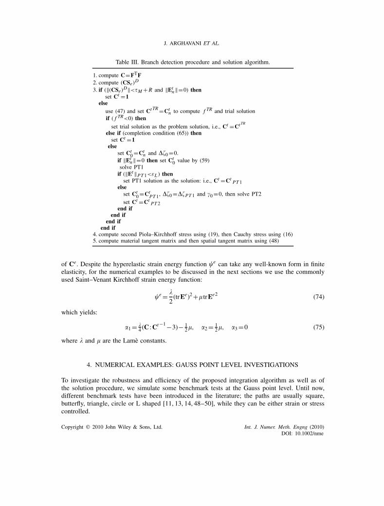
Table III finally presents the proposed solution algorithm based on the logarithmic form of thetime-discrete evolution equation (54) and a Nucleation–Consistent Completion (NC2) scheme.

Implementing the proposed solution procedure, we obtain a robust time integration algorithm; inthe next sections we test its robustness for different complicated stress–strain histories and variousboundary value problems.

RemarkUntil now, the relations have been derived in a completely general manner without specifyingthe form of the Helmholtz free energy �e, apart from the fact that it is an isotropic function


J. ARGHAVANI ET AL.

Table III. Branch detection procedure and solution algorithm.

1. compute C=FTF2. compute (CSe)D

3. if (‖(CSe)D‖<�M +R and ‖Etn‖=0) then

set Ct =1else

use (47) and set Ct TR=Ctn to compute f TR and trial solution

if ( f TR<0) thenset trial solution as the problem solution, i.e., Ct =CtTR

else if (completion condition (65)) thenset Ct =1

elseset Ct

0=Ctn and ��0=0.

if ‖Etn‖=0 then set Ct

0 value by (59)solve PT1if (‖Et‖PT 1<εL ) thenset PT1 solution as the solution: i.e., Ct =Ct

PT 1elseset Ct

0=CtPT 1, ��0=��PT 1 and �0=0, then solve PT2

set Ct =CtPT 2

end ifend if

end ifend if

4. compute second Piola–Kirchhoff stress using (19), then Cauchy stress using (16)5. compute material tangent matrix and then spatial tangent matrix using (48)

of Ce. Despite the hyperelastic strain energy function �e can take any well-known form in finiteelasticity, for the numerical examples to be discussed in the next sections we use the commonlyused Saint–Venant Kirchhoff strain energy function:

�e=

2(trEe)2+� trEe2 (74)

which yields:

�1= 4 (C :Ct−1−3)− 1

2�, �2= 12�, �3=0 (75)

where and � are the Lamè constants.

4. NUMERICAL EXAMPLES: GAUSS POINT LEVEL INVESTIGATIONS

To investigate the robustness and efficiency of the proposed integration algorithm as well as ofthe solution procedure, we simulate some benchmark tests at the Gauss point level. Until now,different benchmark tests have been introduced in the literature; the paths are usually square,butterfly, triangle, circle or L shaped [11, 13, 14, 48–50], while they can be either strain or stresscontrolled.



We first investigate the simple shear test, a well-known benchmark test for evaluating a finite-strain model. Then, we simulate some uniaxial stress-controlled tension-compression and torsiontests at three different temperatures, varying from PE to shape memory effect. Afterward, a(E11−E22)-controlled butterfly-shaped and a (E11−E12)-controlled square-shaped path are simu-lated. In each simulation we consider two different maximum values for controlling variables aswell as two different temperatures, one leading to PE and the other to shape memory effect. Finally,we present the response paths for stress-controlled butterfly- and square-shaped paths.††

In order to investigate the algorithm robustness, two different time step sizes are adopted in eachnumerical test. Moreover, we report the average number of iterations in PT1 and PT2 for differentselected cases to show the convergence behavior (as this information can somehow be related tothe algorithm robustness). Averages are computed by dividing the total number of iterations in atest by the total number of calls to the corresponding subroutine.

While we report the results for the logarithmic form of the evolution equation when a NC2scheme is adopted in the solution algorithm, we also investigate the convergence behavior forboth exponential and logarithmic forms of the evolution equation using both regularized (Reg) andNC2 schemes in the solution algorithm.‡‡ Using this approach, it is possible to compare the localconvergence behavior as well as the robustness of different algorithms.

The following material properties, typical of NiTi (see, e.g. [52]), are adopted in all the simu-lations of this paper:

E = 51700MPa, �=0.3, h=750MPa, εL =7.5%

� = 5.6MPaC−1, T0=−25◦C, R=140MPa, A f =0◦C, M f =−25◦C

where E and � are the elastic modulus and the Poisson ratio, respectively. Details on the materialparameters identification can be found in [53].

4.1. Simple shear test

We start simulating a loading-unloading simple shear test at two different temperatures: 37◦C forPE and −25◦C for shape memory effect (see Figure 1, left). The deformation gradient and theGreen–Lagrange strain tensors are expressed in terms of the shear amount as follows:

F=

⎡⎢⎣1 0

0 1 0

0 0 1

⎤⎥⎦ , E= 1

2

⎡⎢⎢⎣0 0

2 0

0 0 0

⎤⎥⎥⎦

Figure 1 (right) shows the results for two different time step sizes (0.02 s and 0.2 s denoted by theline and the circle symbols, respectively, while the total simulation time is 2 s). The results showthe algorithm accuracy as well as the robustness for large time step sizes. We also observe themodel capability of capturing PE as well as shape memory effect.

††We remark that, in this section, we use as a strain measure the Green–Lagrange strain tensor and as a stressmeasure the second Piola–Kirchhoff stress tensor. Moreover, we highlight that reported results are not physical aswe know that the selected measures are not physical measures (see for example [51]).

‡‡Following this procedure, we consider four different cases: a regularized scheme with exponential mapping(exp+Reg), a nucleation–completion scheme with exponential mapping (exp+NC2), a regularized scheme withlogarithmic mapping (log+Reg) and a nucleation–completion scheme with logarithmic mapping (log+NC2).


J. ARGHAVANI ET AL.

1

κ

0 2 4 6 8 10 12 14

0

100

200

300

400

500

κ [ % ]

S12

[ M

Pa

]

T = 37° C

° C

Figure 1. Simple shear test: shear deformation (left) and S12 component as a function of the shear amount (right). Lines denote dt=0.02s and the circles dt =0.2s.

4.2. Uniaxial tests

We now simulate tension-compression as well as torsion tests under stress control at three differenttemperatures, and in particular for T>A f , M f <T<A f , and T<M f . For the tests with T<A fwe also investigate shape recovery under temperature control. Moreover, we remark that since theterm �M uses Macaulay brackets, the predictions of any temperature equal to or below M f wouldbe the same.

Figure 2 reports the stress–strain response with a solid line and for the tests with T<A f , thestrain recovery with a dashed line. The results show the model capability of capturing PE andshape memory effect as well as the intermediate behavior.

To check the algorithm robustness, we perform the tests with two different stress increments perstep: in particular we consider stress increments equal to 150 and 15MPa in tension-compressiontests and equal to 100 and 10MPa in torsion tests. Points A and B in Figure 2, indicate that aload cutting is used in the global solution (equilibrium) to prevent its divergence as the stiffness isabruptly changing.§§ Table IV shows the convergence results for different formulations in tension-compression tests. We use letters f and c to distinguish the results for the fine and coarseincrements, respectively. For each case, a pair of numbers is reported corresponding to PT1 andPT2, respectively. As it is expected, using a NC2 scheme reduces the average number of iterations.It is interesting to note that using the logarithmic form reduces the number of iterations and thiscan be interpreted as the result of the reduced nonlinearity of the equations. We do not focus onthe efficiency comparison in this section and postpone it to Section 5, where we compare the CPUtime for different boundary value problems (BVPs).

4.3. Multiaxial tests

We now investigate two types of strain-controlled biaxial tests, the first consisting of a butterfly-shaped (E11−E22) input, and the second of a square-shaped (E11−E12) input. Figure 3 shows thestrain input as well as the stress output for the butterfly-shaped test. The plots on the left refer to astrain value of 6%, while a 10% strain value is used for plots on the right. The middle and lower

§§Similar to increment cutting technique, we can use load-cutting for a stress-controlled problem.



0 2 4 6 8 10

0

500

1000

1500

E11

[ % ]

S11

[ M

Pa

]A

B

T = 37° C

0 2 4 6 8

0

500

1000

E12

[ % ]

S12

[ M

Pa

]

B

B

T = 37° C

0 2 4 6 8 10

0

200

400

600

800

E11

[ % ]

S11

[ M

Pa

]

° C

B

A

0 2 4 6 8

0

125

250

375

500

E12

[ % ]

S12

[ M

Pa

]

° C

A

BA

0 2 4 6 8

0

200

400

600

E11

[ % ]

S11

[ M

Pa

]

° CA

A

0 2 4 6 8

0

100

200

300

400

E12

[ % ]

S12

[ M

Pa

]

° CA

A

Figure 2. Uniaxial tests: tension-compression tests (left) and torsion tests (right) under stresscontrol: T =37◦C (upper); T =−5◦C (center); T =−25◦C (lower). For T<A f strain recoveryinduced by heating is indicated with a dashed-dot line. Stress increment per step duringtension-compression tests: 15MPa (line) and 150MPa (circles). Stress increment per step

during torsion tests: 10MPa (line) and 100MPa (circles).

plots show the results at T =37◦C (PE) and T =−25◦C (shape memory effect), respectively. Allseries of tests are performed using two different time step sizes (0.02s and 0.2s, corresponding tothe solid line and the circle symbols, respectively), while the total time is 8s.

As we discussed in Section 3.2, the implemented algorithm, detects any divergence duringa solution process and automatically cuts the increment size. We use a label IC to indicate an


J. ARGHAVANI ET AL.

Table IV. Convergence results for tension-compression tests.

exp+Reg exp+NC2 log+Reg log+NC2

37◦C ( f ) 6 7 4 44 4 4 4

37◦C (c) 8 7 4 44 4 4 4

−5◦C ( f ) 8 4 4 45 4 4 4

−5◦C (c) 6 6 4 44 5 4 4

−25◦C ( f ) 6 5 4 44 4 4 4

−25◦ C (c) 5 4 4 44 4 4 4

increment in which cutting takes place and emphasize that the increment size is not the actualsize. We avoid reporting intermediate increment results to keep the figures as clear and simple aspossible.

We repeat with a similar approach the squared-shape test and report the results in Figure 4.Tables V and VI show the convergence results for the stain-controlled biaxial tests. For brevity, weonly report the results for the most critical cases, i.e. for 10% strain. It is observed that in termsof convergence, the NC2 scheme is preferred compared with the Reg scheme. As we expected,using a logarithmic form of the evolution equation improves the convergence behavior. Usingthe logarithmic form improves both the robustness and the efficiency by decreasing the equationnonlinearity and the number of increment cuttings, as well as the number of iterations.

We also repeat the above-mentioned tests under stress control. The stress values vary between±700MPa. At T =−25◦C, after applying the stress path, we increase the temperature up to A f ,such that the residual strain recovery takes place as shown in the lower part of Figure 5 (see thedotted line).

5. NUMERICAL EXAMPLES: BOUNDARY VALUE PROBLEMS

In this section, we solve four boundary value problems to validate the adopted model as well asthe proposed integration algorithm and the solution procedure. A helical spring and a medical stentare simulated at two different temperatures to show the model capability of capturing both thePE and shape memory effect. Moreover, we compare the CPU time for both the exponential andlogarithmic forms of the time-discrete evolution equation, as well as for Reg and NC2 schemes. Inall boundary value examples we use the same material properties as in Section 4. The temperaturein pseudo-elastic simulations is set to 37◦C while in shape memory effect simulations a temperatureof −25◦C is adopted.

For all simulations, we use the commercial nonlinear finite element software ABAQUS/Standard,implementing the described algorithm within a user-defined subroutine UMAT.



0 2 4 6

0

2

4

6

E11

[ % ]

E22

[ %

]

0 5 10

0

5

10

E11

[ % ]

E22

[ %

]

0 1000 2000

0

1000

2000

S11

[ MPa ]

S22

[ M

Pa

]

T = 37° C

0 2000 4000 6000

0

2000

4000

6000

S11

[ MPa ]

S22

[ M

Pa

]

T = 37° C

IC

0 1000 2000

0

1000

2000

S11

[ MPa ]

S22

[ M

Pa

]

° C

0 2000 4000 6000

0

2000

4000

6000

S11

[ MPa ]

S22

[ M

Pa

]

° C

IC

Figure 3. Biaxial butterfly-shaped input under strain control up to 6% (upper-left) and10% (upper-right); stress output at T =37◦C (center) and T =−25◦C (lower) for two

time step sizes: 0.02 s (line) and 0.2 s (circles).

5.1. Helical spring: pseudo-elastic test

A helical spring (with a wire diameter of 4mm, a spring external diameter of 24mm, a pitch sizeof 12mm and with two coils and an initial length of 28mm) is simulated using 9453 quadratictetrahedron (C3D10) elements and 15 764 nodes. An axial force of 1525N is applied to the oneend while the other end is completely fixed. The force is increased from zero to its maximumvalue and unloaded back to zero. Figure 6 shows the spring initial geometry, the adopted mesh andthe deformed shape under the maximum force. After unloading, the spring recovers its originalshape as it is expected in the pseudo-elastic regime. Figure 7 (left) shows the force–displacementdiagram. It is observed that the spring shape is fully recovered after load removal.


J. ARGHAVANI ET AL.

0 2 4 6

0

2

4

6

E11

[ % ]

E12

[ %

]

0 5 10

0

5

10

E11

[ % ]

E12

[ %

]

0 500 1000

0

500

1000

S11

[ MPa ]

S12

[ M

Pa

]

T = 37° C

0 1000 2000 3000

0

1000

2000

3000

S11

[ MPa ]

S12

[ M

Pa

]

ICIC

T = 37° C

ICIC

0 500 1000

0

500

1000

S11

[ MPa ]

S12

[ M

Pa

]

° C

0 1000 2000 3000

0

1000

2000

3000

S11

[ MPa ]

S12

[ M

Pa

]

° CIC

ICIC

IC

IC

Figure 4. Biaxial squared-shaped input under strain control up to 6% (upper-left) and10% (upper-right); stress output at T =37◦C (center) and T =−25◦C (lower) for two

time step sizes: 0.02 s (line) and 0.2 s (circles).

5.2. Helical spring: shape memory effect test

We also simulate the same spring of Section 5.1 in the case of shape memory effect. An axialforce of 427N is applied at T =−25◦C (Figure 8, top) and, after unloading, the spring does notrecover its initial shape (Figure 8, bottom). After heating, up to a temperature of 10◦C, the springrecovers its original shape. Figure 7 (right) shows the force–displacement–temperature behavior.According to Figure 7 (right), heating the spring leads to full recovery of the original shape atT = A f (0◦C) and subsequent heating does not change any more its shape.



Table V. Convergence results for the butterfly-shaped path: up to 10% strain.


37◦C ( f ) 8 8 6 611 11 10 10

37◦C (c) 11 8 10 79 10 9 10

−25◦C ( f ) 7 7 6 610 10 10 10

−25◦C (c) 7 7 7 710 9 10 9

Table VI. Convergence results for the squared-shaped path: up to 10% strain.


37◦C ( f ) 9 9 8 812 12 12 12

37◦C (c) 9 9 8 88 7 7 7

−25◦C ( f ) 13 13 9 914 14 12 11

−25◦C (c) 9 9 9 912 13 13 13

5.3. Crimping of a medical stent: pseudo-elastic test

In this example, the crimping of a pseudo-elastic medical stent is simulated. To this end a medicalstent with 0.216mm thickness and an initial outer diameter of 6.3mm (Figure 9, upper-left) iscrimped to an outer diameter of 1.5mm. Utilizing the ABAQUS/Standard contact module, thecontact between the catheter and the stent is considered in the simulation. A radial displacementis applied to the catheter and is then released to reach the initial diameter. In this process, the stentrecovers its original shape after unloading. Figure 9 (upper-right) shows the stent deformed shapewhen crimped.

5.4. Crimping of a medical stent: shape memory effect test

In this example, the same stent is crimped at a temperature of −25◦C as it is shown in Figure 9(center). Owing to the low temperature, while the catheter is expanded, the stent remains in adeformed state as shown in Figure 9 (lower). The initial shape is however recovered after heating.

5.5. Comparison of CPU times

We now compare the CPU times to show the efficiency gained by using logarithmic form as wellas a nucleation–completion scheme. We remark that we normalize all CPU times with respect tothe CPU time for the case of exponential form with a regularized scheme.


J. ARGHAVANI ET AL.

0 200 400 600 800

0

200

400

600

800

S11

[ MPa ]

S22

[ M

Pa

]

0 200 400 600 800

0

200

400

600

800

S11

[ MPa ]

S12

[ M

Pa

]

0 2 4 6 8

0

2

4

6

8

10

E11

[ % ]

E22

[ %

]

T = 37° C

0 2 4 6 8 10

0

2

4

6

8

E11

[ % ]

E12

[ %

] T = 37° C

0 2 4 6 8

0

2

4

6

8

10

E11

[ % ]

E22

[ %

]

° C

0 2 4 6 8 10

0

2

4

6

8

E11

[ % ]

E12

[ %

]

° C

Figure 5. Biaxial butterfly-shaped input (upper-left) and squared-shaped input (upper-right) under stresscontrol; strain output at T =37◦C (center) and T =−25◦C (lower); strain output (lower) with strain

recovery (dotted line) under temperature increment.

+6.156e+01+4.221e+02+7.827e+02+1.143e+03+1.504e+03+1.864e+03+2.225e+03+2.586e+03+2.946e+03+3.307e+03+3.667e+03+4.028e+03+4.388e+03

Figure 6. Pseudo-elastic spring: comparison of initial geometry and deformed configuration.



0 10 20 30 40 50 60 70 800

200

400

600

800

1000

1200

1400

1600

Displacement [ mm ]

For

ce

[ N ]

T = 37° C

020

4060

80

0510

0

100

200

300

400

500

Temperature [ °C ]Displacement [ mm ]

For

ce

[ N ]

Figure 7. Force–displacement diagram for the SMA spring: PE (left) and shape memory effect (right).

+2.640e+01+2.048e+02+3.832e+02+5.616e+02+7.400e+02+9.184e+02+1.097e+03+1.275e+03+1.454e+03+1.632e+03+1.810e+03+1.989e+03+2.167e+03

+1.272e-01+1.264e+02+2.527e+02+3.789e+02+5.052e+02+6.314e+02+7.577e+02+8.840e+02+1.010e+03+1.137e+03+1.263e+03+1.389e+03+1.515e+03

Figure 8. Shape memory effect in the simulated spring: deformed shape undermaximum load (top) and after unloading (bottom).

We first consider the CPU times for the SME simulations to study the effect of different time-discrete forms. Owing to the small-elastic regime than in the PE case, we expect approximately thesame CPU times for both Reg and NC2 schemes. Therefore, these tests give us an approximationof the gained efficiency due to the use of the logarithmic form of the time-discrete evolutionequation. Comparing the simulation CPU times for exponential and logarithmic forms for SMEcases reported in Table VII, we conclude that using the logarithmic form decreases CPU time ofapproximately 20% compared with the exponential form.

We now consider the CPU times for PE simulations. As it can be observed in Table VII, inall cases, using the NC2 scheme decreases the CPU time compared with the Reg scheme. Thisdecrease depends on the problem and for the simulated problems it varies from 6% (spring andlog form) to 21% (stent and log form).


J. ARGHAVANI ET AL.

(Avg: 75%)

+3.007e+01+3.190e+02+6.080e+02+8.970e+02+1.186e+03+1.475e+03+1.764e+03+2.053e+03+2.342e+03+2.631e+03+2.920e+03+3.209e+03+3.498e+03

+1.116e+01+1.933e+02+3.754e+02+5.575e+02+7.396e+02+9.217e+02+1.104e+03+1.286e+03+1.468e+03+1.650e+03+1.832e+03+2.014e+03+2.196e+03

+7.937e+00+9.015e+01+1.724e+02+2.546e+02+3.368e+02+4.190e+02+5.012e+02+5.834e+02+6.657e+02+7.479e+02+8.301e+02+9.123e+02+9.945e+02

Figure 9. Stent crimping: initial geometry (upper-left), crimped shape in PE case (upper-right), crimpedshape in SME case (center) and deformed shape in SME case after uncrimping (lower).



Table VII. CPU times comparison.


Stent (PE) 1.00 0.84 0.81 0.64Spring (PE) 1.00 0.89 0.74 0.70Stent (SME) 1.00 1.01 0.81 0.81Spring (SME) 1.00 1.02 0.79 0.77

We finally compare the CPU time of the proposed integration algorithm (log+NC2) with thepreviously proposed one (exp+Reg). Considering the first and last columns of Table VII, weobserve that the gained efficiency varies from 19% up to 36%.

6. SUMMARY AND CONCLUSIONS

In this paper, we investigate a 3D finite-strain constitutive model and propose a robust and efficienttime-integration algorithm. We introduce a well-defined form for model variables as well as anucleation–consistent completion scheme to avoid extensively used regularization schemes. Wealso discuss the choice of suitable initial guesses in the Newton–Raphson method.

Moreover, we introduce a logarithmic mapping and propose a new form of the time-discreteevolution equation. Studying different benchmark problems at the gauss point level, we showthe robustness of the proposed algorithm. Implementing the proposed integration algorithmwithin a user-defined subroutine (UMAT) in the commercial nonlinear finite element softwareABAQUS/Standard, we also solve different boundary value problems. Comparing the CPU times,we show the robustness as well as the efficiency (in the order of 25%) of the proposed timeintegration and solution algorithm.

APPENDIX A

In this Appendix, we present the linearized form of Equation (56). To this end, we define thefollowing second-order tensors:

U=Ut−1, C=Ct−1

, Q=��UAU, G=exp(Q), W=UCnU, H= log(W) (A1)

and the following fourth-order tensors:

U = �U�Ct

, U= �U�Ct

, C= �C�Ct

, S= �S�Ct

, X= �X�Ct

Y = �Y�Ct

, A= �A�Ct

, Q= �Q�Ct

, W= �W�Ct

, G= �G�Q

H = �H�W

, S= �S�C

, Y= �Y�C

, A= �A�C

(A2)


J. ARGHAVANI ET AL.

with components [54]:

Xijkl = 12hIijkl+ 1

2 (�M +�)Nijkl

Sijkl = 12CmnklCmnCij+2�1Cijkl+2�2CimklCmnCnj+2�2CimCmnCnjkl

Yijkl = CimSmjkl−Iimkl Xmj−CtimXmjkl

Aijkl = 2Zimpq(Ypqkl− 13Ynnklpq)C

tmj+2ZimImjkl

Qijkl = ��Uimkl AmnUnj+��UimAmnUnjkl+��UimAmnklUnj

Wijkl = Uirkl(Cn)rsUsm+Uir(Cn)rsUsjkl

Sijkl = 12CijCkl+2�2CimImnklCnj

Yijkl = CimSmjkl+IimklSmj

Aijkl = 2Zimpq(Ypqkl− 13Ynnklpq)C

tmj

(A3)

where,

N= 1

‖Et‖ (I−N⊗N), Z= 1

‖YD‖ (I−Z⊗ZT) (A4)

and

N= Et

‖Et‖ , Z= YD

‖YD‖ (A5)

We compute the components of tensors U, U, C, G, H as well as U, U, C, G and H throughspectral decomposition and refer the readers to [55] to see how it can be done. The componentsof the forth-order identity tensor I are defined as:

Iijkl= 12ikjl+ 1

2iljk (A6)

We now present the linearized form of Equations (56) as [54]:

(R11)ijkl = ��Aijkl

(R12)ijkl = UimklHmnUnj+UimHmnUnjkl+UimHmnklUnj+��Aijkl

(R13)ij = Aij

(R14)ij = −2��ZimpqCtmj(C

tpnNnq− 1

3CtklNklpq)

(R21)ij = ZnmYmnij, (R22)ij= ZnmYmnij, R23 =0, R24=−ZijCtimNmj

(R31)ij = 0, (R32)ij= 12Nij, R33=0, R34 =0

(A7)

where

R11 = Rt,C, R12=Rt

,Ct , R13=Rt,��, R14=Rt

,�

R21 = R�,C, R22= R�

,Ct , R23 = R�,��, R24 = R�

,�

R31 = R�,C, R32= R�

,Ct , R33 = R�,��, R34 = R�

,�

(A8)



In order to linearize the time-discrete evolution equation in the exponential form, we derive thelinearized form of Equation (52) as follows [54]:

(R11)ijkl = ��UimGmnpqArsklUnjUprUsq

(R12)ijkl = UimklGmnUnj+UimGmnklUnj+UimGmnUnjkl

(R13)ij = UimUmnUpqUrj AnpGqr

(R14)ij = −2��UimUnjGmnpqUprUsqZrmpqCtms(C

tpnNnq− 1

3CtklNklpq)

(A9)

ACKNOWLEDGEMENTS

J. Arghavani has been partially supported by Iranian Ministry of Science, Research and Technology, andpartially by Dipartimento di Meccanica Strutturale, Università degli Studi di Pavia.

F. Auricchio and A. Reali have been partially supported by the Cariplo Foundation through the projectnumber n.2009.2822; by the Ministero dell’Istruzione, dell’Università e della Ricerca through the projectn. 2008MRKXLX; and by the European Research Council through the Starting Independent ResearchGrant BioSMA: Mathematics for Shape Memory Technologies in Biomechanics.

REFERENCES

1. Otsuka K, Wayman CM. Shape Memory Materials. Cambridge University Press: Cambridge, 1998.2. Duerig TW, Melton KN, Stoekel D, Wayman CM. Engineering Aspects of Shape Memory Alloys. Butterworth-

Heinemann: London, 1990.3. Duerig T, Pelton A, Stöckel D. An overview of nitinol medical applications. Materials Science and Engineering

A 1999; 273–275:149–160.4. Kuribayashi K, Tsuchiya K, You Z, Tomus D, Umemoto M, Ito T, Sasaki M. Self-deployable origami stent

grafts as a biomedical application of Ni-rich TiNi shape memory alloy foil. Materials Science and Engineering:A 2006; 419(1–2):131–137.

5. Funakubo H. Shape Memory Alloys. Gordon and Breach Science Publishers: New York, 1987.6. Raniecki B, Lexcellent C. Rl-models of pseudoelasticity and their specifications for some shape memory solids.

European Journal of Mechanics—A/Solids 1994; 13:21–50.7. Raniecki B, Lexcellent C. Thermodynamics of isotropic pseudoelasticity in shape memory alloys. European

Journal of Mechanics—A/Solids 1998; 17(2):185–205.8. Panico M, Brinson L. A three-dimensional phenomenological model for martensite reorientation in shape memory

alloys. Journal of the Mechanics and Physics of Solids 2007; 55(11):2491–2511.9. Souza AC, Mamiya EN, Zouain N. Three-dimensional model for solids undergoing stress-induced phase

transformations. European Journal of Mechanics—A/Solids 1998; 17(5):789–806.10. Helm D, Haupt P. Shape memory behaviour: modelling within continuum thermomechanics. International Journal

of Solids and Structures 2003; 40(4):827–849.11. Helm D. Formgedächtnislegierungen–experimentelle untersuchung, phänomenologische modellierung und

numerische simulation der thermomechanischen materialeigenschaften. Ph.D. Thesis, UniversitatGesamthochschule Kassel, 2001.

12. Arghavani J, Auricchio F, Naghdabadi R, Reali A, Sohrabpour S. A 3-D phenomenological constitutive modelfor shape memory alloys under multiaxial loadings. International Journal of Plasticity 2010; 26:976–991.

13. Auricchio F, Petrini L. Improvements and algorithmical considerations on a recent three-dimensional modeldescribing stress-induced solid phase transformations. International Journal for Numerical Methods in Engineering2002; 55(11):1255–1284.

14. Auricchio F, Petrini L. A three-dimensional model describing stress-temperature induced solid phasetransformations: thermomechanical coupling and hybrid composite applications. International Journal forNumerical Methods in Engineering 2004; 61(5):716–737.


J. ARGHAVANI ET AL.

15. Auricchio F, Petrini L. A three-dimensional model describing stress-temperature induced solid phasetransformations: solution algorithm and boundary value problems. International Journal for Numerical Methodsin Engineering 2004; 61(6):807–836.

16. Thiebaud F, Lexcellent C, Collet M, Foltete E. Implementation of a model taking into account the asymmetrybetween tension and compression, the temperature effects in a finite element code for shape memory alloysstructures calculations. Computational Materials Science 2007; 41(2):208–221.

17. Helm D. Numerical simulation of martensitic phase transitions in shape memory alloys using an improvedintegration algorithm. International Journal for Numerical Methods in Engineering 2007; 69(11):1997–2035.

18. Bouvet C, Calloch S, Lexcellent C. A phenomenological model for pseudoelasticity of shape memory alloysunder multiaxial proportional and nonproportional loadings. European Journal of Mechanics—A/Solids 2004;23(1):37–61.

19. Qidwai MA, Lagoudas DC. On thermomechanics and transformation surfaces of polycrystalline niti shape memoryalloy material. International Journal of Plasticity 2000; 16(10–11):1309–1343.

20. Lagoudas DC, Entchev PB. Modeling of transformation-induced plasticity and its effect on the behavior ofporous shape memory alloys. Part I: constitutive model for fully dense smas. Mechanics of Materials 2004;36(9):865–892.

21. Auricchio F, Reali A, Stefanelli U. A three-dimensional model describing stress-induced solid phase transformationwith permanent inelasticity. International Journal of Plasticity 2007; 23(2):207–226.

22. Popov P, Lagoudas DC. A 3-D constitutive model for shape memory alloys incorporating pseudoelasticity anddetwinning of self-accommodated martensite. International Journal of Plasticity 2007; 23(10–11):1679–1720.

23. Moumni Z, Zaki W, Nguyen QS. Theoretical and numerical modeling of solid-solid phase change: applicationto the description of the thermomechanical behavior of shape memory alloys. International Journal of Plasticity2008; 24(4):614–645.

24. Auricchio F, Sacco E. Thermo-mechanical modelling of a superelastic shape-memory wire under cyclic stretching-bending loadings. International Journal of Solids and Structures 2001; 38(34–35):6123–6145.

25. Auricchio F, Taylor RL. Shape-memory alloys: modelling and numerical simulations of the finite-strain superelasticbehavior. Computer Methods in Applied Mechanics and Engineering 1997; 143(1–2):175–194.

26. Auricchio F. A robust integration-algorithm for a finite-strain shape-memory-alloy superelastic model. InternationalJournal of Plasticity 2001; 17(7):971–990.

27. Pethö A. Constitutive modelling of shape memory alloys at finite strain. Journal of Applied Mathematics andMechanics (ZAMM) 2001; 81(52):355–356.

28. Ziolkowski A. Three-dimensional phenomenological thermodynamic model of pseudoelasticity of shape memoryalloys at finite strains. Continuum Mechanics and Thermodynamics 2007; 19(6):379–398.

29. Helm D. Thermomechanics of martensitic phase transitions in shape memory alloys. Part i: constitutive theoriesfor small and large deformations. Journal of Mechanics of Materials and Structures 2007; 2(1):87–112.

30. Reese S, Christ D. Finite deformation pseudo-elasticity of shape memory alloys—constitutive modelling andfinite element implementation. International Journal of Plasticity 2008; 24(3):455–482.

31. Christ D, Reese S. A finite element model for shape memory alloys considering thermomechanical couplings atlarge strains. International Journal of Solids and Structures 2009; 46(20):3694–3709.

32. Evangelista V, Marfia S, Sacco E. A 3D SMA constitutive model in the framework of finite strain. InternationalJournal for Numerical Methods in Engineering 2009; DOI: 10.1002/nme.2717.

33. Thamburaja P. A finite-deformation-based phenomenological theory for shape-memory alloys. InternationalJournal of Plasticity 2010; DOI: 10.1016/j.ijplas.2009.12.004.

34. Arghavani J, Auricchio F, Naghdabadi R, Reali A, Sohrabpour S. A 3D finite strain phenomenological constitutivemodel for shape memory alloys considering martensite reorientation. Continuum Mechanics and Thermodynamics,DOI: 10.1007/s00161-010-0155-8.

35. Müller C, Bruhns O. A thermodynamic finite-strain model for pseudoelastic shape memory alloys. InternationalJournal of Plasticity 2006; 22(9):1658–1682.

36. Thamburaja P. Constitutive equations for martensitic reorientation and detwinning in shape-memory alloys. Journalof the Mechanics and Physics of Solids 2005; 53(4):825–856.

37. Stupkiewicz S, Petryk H. Finite-strain micromechanical model of stress-induced martensitic transformations inshape memory alloys. Materials Science and Engineering A 2006; 438–440:126–130.

38. Pan H, Thamburaja P, Chau F. Multi-axial behavior of shape-memory alloys undergoing martensitic reorientationand detwinning. International Journal of Plasticity 2007; 23(4):711–732.

39. Stein E, Sagar G. Theory and finite element computation of cyclic martensitic phase transformation with finitestrain. International Journal for Numerical Methods in Engineering 2008; 74:1–31.



40. Lubarda VA. Elastoplasticity Theory. CRC Press: Boca Raton, 2001.41. Haupt P. Continuum Mechanics and Theory of Materials. Springer: New York, 2002.42. Vladimirov IN, Pietryga MP, Reese S. On the modelling of non-linear kinematic hardening at finite strains

with application to springback-comparison of time integration algorithms. International Journal for NumericalMethods in Engineering 2008; 75(1):1–28.

43. Auricchio F, Reali A, Stefanelli U. A macroscopic 1D model for shape memory alloys including asymmetricbehaviors and transformation-dependent elastic properties. Computer Methods in Applied Mechanics andEngineering 2009; 198(17–20):1631–1637.

44. Belytschko T, Liu WK, Moran B. Nonlinear Finite Elements for Continua and Structures. Wiley: New York,2000.

45. Eterovic AL, Bathe KJ. A hyperelastic-based large strain elasto-plastic constitutive formulation with combinedisotropic-kinematic hardening using the logarithmic stress and strain measures. International Journal for NumericalMethods in Engineering 1990; 30(6):1099–1114.

46. Miehe C. Exponential map algorithm for stress updates in anisotropic multiplicative elastoplasticity for singlecrystals. International Journal for Numerical Methods in Engineering 1996; 39(19):3367–3390.

47. Vladimirov IN, Pietryga MP, Reese S. Anisotropic finite elastoplasticity with nonlinear kinematic andisotropic hardening and application to sheet metal forming. International Journal of Plasticity 2009; DOI:10.1016/j.ijplas.2009.09.008.

48. Lim TJ, McDowell DL. Mechanical behavior of an Ni–Ti shape memory alloy under axial-torsional proportionaland nonproportional loading. Journal of Engineering Materials and Technology 1999; 121:9–18.

49. Sittner P, Hara Y, Tokuda M. Experimental study on the thermoelastic martensitic transformation in shapememory alloy polycrystal induced by combined external forces. Metallurgical and Materials Transactions A1995; 26:2923–2935.

50. Grabe C, Bruhns O. Path dependence and multiaxial behavior of a polycrystalline niti alloy within the pseudoelasticand pseudoplastic temperature regimes. International Journal of Plasticity 2009; 25:513–545.

51. Pai PF, Palazotto AN, Greer Jr JM. Polar decomposition and appropriate strains and stresses for nonlinearstructural analyses. Computers and Structures 1998; 66(6):823–840.

52. URL Available from: www.shape-memory-alloys.com.53. Auricchio F, Coda A, Reali A, Urbano M. Sma numerical modeling versus experimental results: Parameter

identification and model prediction capabilities. Journal of Materials Engineering and Performance 2009;18(5–6):649–654.

54. Arghavani J. Thermomechanical behavior of shape memory alloys under nonproportional loading: constitutivemodelling and numerical inplementation in small and finite strains. Ph.D. Thesis, Sharif University of Technology,Iran, 2010.

55. de Souza Neto EA. On general isotropic tensor functions of one tensor. International Journal for NumericalMethods in Engineering 2004; 61:880–895.


on the robustness and efficiency of integration algorithms for a 3d

Documents