HAL Id: hal-03330337https://hal.archives-ouvertes.fr/hal-03330337

Submitted on 1 Sep 2021

HAL is a multi-disciplinary open accessarchive for the deposit and dissemination of sci-entific research documents, whether they are pub-lished or not. The documents may come fromteaching and research institutions in France orabroad, or from public or private research centers.

L’archive ouverte pluridisciplinaire HAL, estdestinée au dépôt et à la diffusion de documentsscientifiques de niveau recherche, publiés ou non,émanant des établissements d’enseignement et derecherche français ou étrangers, des laboratoirespublics ou privés.

On the relationship between battery power capacitysizing and solar variability scenarios for industrial

off-grid power plantsLouis Polleux, Thierry Schuhler, Gilles Guerassimoff, Jean-Paul Marmorat,

John Sandoval, Sami Ghazouani

To cite this version:Louis Polleux, Thierry Schuhler, Gilles Guerassimoff, Jean-Paul Marmorat, John Sandoval, et al.. Onthe relationship between battery power capacity sizing and solar variability scenarios for industrial off-grid power plants. Applied Energy, Elsevier, 2021, 302, pp.117553. �10.1016/j.apenergy.2021.117553�.�hal-03330337�

On the relationship between battery power capacity sizing and solar variability scenarios for industrial off-grid power

plants*

Authors: Louis Polleux1,2 , †

, Thierry Schuhler2

, Gilles Guerassimoff1

, Jean-Paul Marmorat1

, John Sandoval2

,

Sami Ghazouani2

1 Center for Applied Mathematics, Mines Paristech PSL, Sophia Antipolis, France

2 Research and Development, TOTAL, Paris, France

Abstract:

Due to its high short-term variability, solar-photovoltaic power in isolated industrial grids faces a challenge

of grid reliability. Storage systems can provide grid support but come at a high cost that requires carefully

evaluating power capacity needs. Battery sizing methodologies are now the focus of many studies, with a

global upward trend in detailed modelling and complex optimization. However, although solar variability

can be the source of uncertainties and battery oversizing, it rarely features as an input in scenarios. This

study proposes several solar variability scenarios thanks to the wavelet-variability model and two variability

metrics. These scenarios are employed as inputs in two sizing methodologies to compare the resulting

battery capacity and draw conclusions on the role of modelling complexity and scenario identification.

Results show that neglecting the photovoltaic power plant smoothing effect leads to an overestimation of

the battery power support of 51%. In the other hand, complex dynamic modelling may reduce the battery

power capacity by 25%. The economic analysis shows that a proper combination of variability scenario

and battery sizing methodology may reduce the levelized costs of electricity by 3%.

Highlights

• Modelling photovoltaic plant geographical smoothing avoids over-investments.

• Identifying variability scenarios is crucial to ensure continuity of supply.

• Combining ramp-detection and variability index spares the use of day-long timeseries.

Keywords

Solar variability, Storage systems, Industrial microgrid, Power quality, Wavelet variability model

Nomenclature

Abbreviations

WVM Wavelet Variability Model

PV Photovoltaic

RDA Ramp detection algorithm

VI Local variability index

GHI Global Horizontal Irradiance

CSI Clear sky irradiance

*

The short version of the paper was presented at ICAE2020, Dec 1-10, 2020. This paper is a substantial extension

of the short version of the conference paper. †

Corresponding author: Louis Polleux louis.polleux@mines-paristech.fr , CMA Mines Paristech, 1 Rue Claude

Daunesse, 06904 Sophia Antipolis

LCOE Levelized costs of electricity

CAPEX Capital expenditure

OPEX Operational expenditure

Symbols

𝑇𝑅 Time-period of PV drop

Δ𝑃𝑅 PV power loss within time interval

𝐿𝐺𝐻𝐼 Euclidean length of GHI curve

Δ𝑡 GHI data sampling interval

𝑃𝑃𝑉 PV power

𝑟𝑟𝑃𝑉 PV power ramp rate

𝑃𝑓𝑜𝑠𝑠𝑖𝑙 Fossil generation active power

𝑃𝐿 Electrical load active power

𝑃𝑢𝑛𝑚𝑒𝑡 𝑙𝑜𝑎𝑑 Unmet load power

𝑟𝑟𝑓𝑜𝑠𝑠𝑖𝑙 Fossil generation total ramp rate

𝑃𝑃𝑉𝑟𝑎𝑡𝑒𝑑 PV plant installed capacity

𝜂𝑃𝑉𝑖𝑛𝑣 PV inverter efficiency

Δ𝑓 Grid frequency shift

Δ𝑃𝑚𝑒𝑐 Mechanical power

𝑀 Inertia constant

D Damping constant

𝐾𝑝, 𝐾𝑖, 𝐾𝑑 Battery controller constants

𝐶𝑏𝑎𝑡 Battery power capacity

𝑃𝑏𝑎𝑡 Battery active power

𝑃𝑏𝑎𝑡∗ Battery power order

𝜂𝑖𝑛𝑣 , 𝜂𝑏𝑎𝑡 Battery and inverter efficiencies

𝑃𝑏𝑎𝑡𝑚𝑖𝑛, 𝑃𝑏𝑎𝑡

𝑚𝑎𝑥 Minimum and maximum battery power

𝐸𝑏𝑎𝑡 Battery energy

𝑆𝑂𝐶𝑚𝑖𝑛, 𝑆𝑂𝐶𝑚𝑎𝑥 Minimum and maximum battery state-of-charge

𝐸𝑏𝑎𝑡𝑚𝑎𝑥 Maximum battery energy

𝛿𝑡 Simulation solving interval

𝜈𝑋 Power quality function

𝛼𝑖 , 𝛽𝑖 Variables for battery dynamic sizing optimization

1 Introduction Recent climate change trajectories and increasing political pressure over carbon legislation have made the

establishment of an efficient low-carbon industry a priority. In its 2019 Outlook, the International Energy

Agency (IEA) highlighted that powering facilities with low-carbon electricity constitutes one the main levers

to achieve the industry’s sustainable transition (1).

In developing countries with unreliable grids or large off-grid areas, industrial facilities must rely on on-

site generation(2) and thus need to install their own renewable power plants to reduce their carbon

emissions (3). In these applications, large-scale industrial microgrids will therefore play a key role.

So far, the need for affordable, reliable electricity has motivated the use of conventional fossil generation

(gas-turbine or internal combustion engines) for electricity production. However, following the sharp drop

in renewable electricity production costs, hybrid power plants featuring fossil generation and renewable

resources are now drawing the attention of the scientific community since. Varying applications are found

in the literature, from industrial microgrids (4) to water-treatment plants (5) and even future oil and gas

platforms(6). Among the wide variety of renewable sources, solar PV is one of the most promising due to

its fast development.

1.1 Challenge of solar PV integration in off-grid industrial power plants The concept of industrial microgrids has not been extensively covered in the literature to date. The main

sectors requiring such systems are the mining industry (7), manufacturing industry (8,9), water treatment

(5) and upstream oil and gas (6). The main characteristics of such systems are:

- High power ratings compared to conventional microgrid systems (from hundreds of kW to several

hundreds of MW).

- Deterministic load profiles depending on the production schedule of the factory with a generally

low level of variability.

- Strict reliability specifications regarding electricity supply for economic and safety reasons.

- Centralized ownership and operation for all production units.

Large scale integration of solar PV power with high short-term variability raises questions about the

reliability and continuity of supply. As highlighted in (10), fossil-fuel generation lacks flexibility (long start-

up time, relatively low ramp-rate, etc.) and limits the renewable energy penetration rate. Additionally,

integration of renewable resources contributes to reduce the mechanical inertia of the system which may

lead to unstable grid and poor resilience to solar perturbation (11).

Storage systems are an effective way to compensate the lack of flexibility of fossil generation (12). Fast

response technologies are the most suited to provide grid support, with an advantage for lithium-ion

technologies considering recent projects and decreasing cost (13). However, storage systems significantly

impact a plant’s economic performance, which is why a deep understanding of solar variability is of

paramount importance to support the development of industrial power plants.

1.2 Assessment of solar variability and its impact on power system

Accurate assessment of solar resources is a topic of growing importance for autonomous energy systems

developers. Many software systems now use solar production profiles to determine optimal investments

in components (14). In (15) for example, the battery power capacity is calculated using hourly on-site

timeseries in order to compensate the lack of generation.

Since grid reliability is a key issue, a deeper analysis must be carried out (16). As frequency fluctuation

occurs at short timescales due to instant power imbalances (17), solar short-term ramps have a strong

impact on the system. Hence, defining solar variability scenarios is critical to determine the size of the

battery system.

The production variability of photovoltaic (PV) systems is a complex phenomenon that is still being

investigated by the scientific community to provide reliable metrics (18) and forecasts (19). Atmospheric

conditions affect clouds’ size, opacity and altitude, and also their horizontal and vertical movements. In

addition, a site’s characteristics, such as its orography, plays an important role in cloud dynamics (18). This

makes the adaptation of variability indexes from one site to another almost impossible. On the other hand,

high on-site resolution irradiance data are rarely available, making it necessary to conduct measurement

campaigns whenever possible.

PV system size also plays a role in the variability since clouds may cast partial shade on the surface of large

plants. In (20) it was shown that the power profile entirely follows the irradiance profile for time-ranges

greater than 10 minutes. As reported in (21), short-term variability is affected by the size, shape and

scattering of a plant. For plants of several megawatts, 1-s, 10-s, and 1-min ramps can be approximately

60%, 40%, and 10% smaller, respectively, than those measured by a pyranometer.

Based on the work of (22), it is possible to simulate the effect of a plant’s geometry on a single-sensor

timeseries thanks to the Wavelet Variability Model (WVM). The risk of solar power ramp can then be

evaluated with more accuracy.

Meanwhile, significant research has studied sizing technique and grid modelling with the aim of improving

and optimizing the sizing of components (23). Battery sizing techniques range from pure energy

compensation to maintain the power balance to a complex representation of the grid dynamics and

frequency fluctuations (24). On the other hand, (25) highlighted that the relevance of performing highly

detailed grid simulation can be challenging when the solar input scenarios have such high uncertainties.

To the best of the authors’ knowledge, no quantitative study has been performed to date to evaluate the

role of accurate solar variability scenarios and storage sizing complexity in final battery capacity

requirements. Additionally, the financial implications of such aspect remain unsettled in the literature.

To address this question, the paper is organized as follows. In section 2, we propose a methodology to

identify a solar variability scenario from a high-resolution irradiance dataset. Then, we apply the WVM to

simulate the smoothing effect of the PV power plant. Two metrics are proposed and combined to identify

day-long and isolated scenarios. In section 3, we present two battery sizing methodologies with a theoretical

background on power systems: power adequacy and dynamic modelling. These two methodologies are

then applied in section 4 using a case study to quantify the role of the variability scenario and sizing method

in the battery capacity requirement. Finally, we draw conclusions in section 5.

2 Addressing PV transients

2.1 Methodology and data

As stated in the introduction, it is always preferable and more accurate to conduct an on-site measurement

campaign. Yet, in the early stages of a project, the high costs and feasibility issues related to installing and

operating a network of sensors prevent developers from obtaining reliable data on-site. A less costly

approach is to use a worst-case referenced dataset. Thanks to the work carried out in (26), where solar

variability zones were evaluated from a set of measurements of nine power plants, the area of Hawaii was

found to be one of the most variable in the world in terms of solar irradiance. This is also confirmed by

the results presented in (27). Taking a worst-case study perspective, in this paper we propose to use the

data collected by NREL in Oahu (28) for variability analysis and battery sizing. Even though the

meteorological behavior cannot be generalized to all regions in the world, we believe that such highly

variable area like Hawaii can be an interesting benchmark for the scientific community.

Figure 1 shows the solar variability scenario identification procedure. After identifying a suitable dataset,

the WVM is applied to the 1-second irradiance profile to simulate the smoothing effect of a 50MW solar

power plant subject to a cloud speed of 20m/sec.

Then, daily variability indexes are calculated to identify the most variable day. In this paper, we propose

two indicators: the number of ramps detected using a ramp-detection algorithm (RDA) and the Variability

Index (VI) derived from the work of J. Stein et al. (29).

Finally, we extract solar input scenarios for battery sizing from the most variable day. For the sake of clarity

and simplicity, it is more convenient to consider solar variability events as typical solar drops (% of PV

power in a defined time interval) rather than using day-long timeseries. Thanks to the RDA, isolated ramp

events are extracted from the day-long timeseries and are used as alternative variability scenarios. The

uncertainties in the measurement of solar irradiance have been neglected since the information was not

made available by data provider.

Figure 1 Scenario identification process

2.2 Quantifying solar variability

2.2.1 Ramp detection algorithm (RDA) Identifying solar ramps is a key step in solar variability analysis. Numerous methods can be implemented

with varying levels of complexity. In (21), the solar profile 1-second derivative is used to evaluate the ramp

rate. This method can be extended to a larger fixed-time window, but this leads to neglect any change in

irradiance within the time interval. In this case, such a method cannot be implemented because the time-

scale of the solar ramp is expected to vary between raw pyranometer data and WVM filtered data. In (30),

a recognition method for irradiance transition was proposed based on moving averaged variations.

Similarly, in this paper we propose to detect solar ramps thanks to a gradient-based adaptative sliding

window.

The RDA detects each ramp with a higher gradient than the trigger value 𝐴 (in W.m-2

.s-1

). The detected

ramp, which is then labelled by its index 𝑅, has two attributes: 𝑇𝑅 the duration of the ramp and Δ𝑃𝑅 the

power loss within the interval. The algorithm is provided in annex.

2.2.2 Variability index (VI) In this study, we employ a variation of the variability index (VI) proposed by J. Stein et. al. in (29). The

original index is calculated following Eq. 1 and can be interpreted as the ratio of the pyranometer global

horizontal irradiance (GHI) measurement curve length over the clear-sky irradiance (CSI) curve length.

The VI calculation proposed in this paper (Eq. 2) is very similar as it only replaces clear-sky irradiance by

the hourly averaged GHI, with the aim of avoiding the use of clear-sky irradiance estimation models that

may introduce additional bias.

𝑉𝐼 =∑ √(𝐺𝐻𝐼𝑡+1 − 𝐺𝐻𝐼𝑡)2 + Δ𝑡2𝑡𝑓

𝑡=𝑡0

∑ √(𝐶𝑆𝐼𝑡+1 − 𝐶𝑆𝐼𝑡)2 + Δ𝑡2𝑡𝑓

𝑡=𝑡0

Eq. 1

𝑉𝐼 =

𝐿𝐺𝐻𝐼

𝐿𝐺𝐻𝐼 Eq. 2

𝐿𝐺𝐻𝐼 and 𝐿𝐺𝐻𝐼 are the euclidean dictance of the 1sec GHI timeseries and hourly averaged GHI timeseries

respectively.

𝐿𝐺𝐻𝐼 = ∑ √(𝐺𝐻𝐼𝑡+1 − 𝐺𝐻𝐼𝑡)2 + Δ𝑡2

𝑡𝑓

𝑡=𝑡0

Eq. 3

𝐿𝐺𝐻𝐼 = ∑ √(𝐺𝐻𝐼ℎ+1 − 𝐺𝐻𝐼ℎ

)2 + 36002

ℎ𝑓

ℎ=ℎ0

Eq. 4

Figure 2 shows three irradiance profiles from the dataset with a VI value and the number of detected

ramps. This shows that the number of ramps and VI in an RDA can give insight on the level of variability.

The value of the VI are different from the indexes processed by Stein et. al. in (29), which range from 0

to 15. This is due to the fact that 1-min resolution data are used in (29), whereas 1-second data are used

in this study, which obviously gives a longer GHI curve.

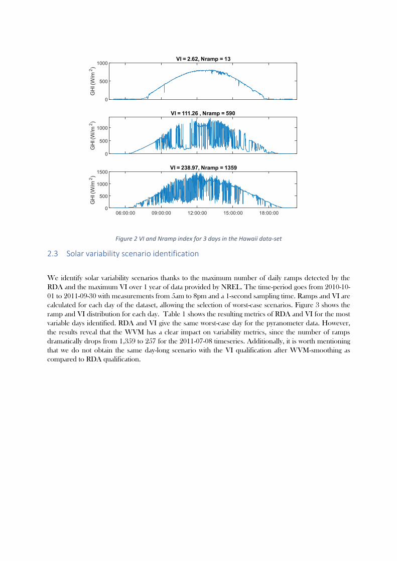
Figure 2 VI and Nramp index for 3 days in the Hawaii data-set

2.3 Solar variability scenario identification

We identify solar variability scenarios thanks to the maximum number of daily ramps detected by the

RDA and the maximum VI over 1 year of data provided by NREL. The time-period goes from 2010-10-

01 to 2011-09-30 with measurements from 5am to 8pm and a 1-second sampling time. Ramps and VI are

calculated for each day of the dataset, allowing the selection of worst-case scenarios. Figure 3 shows the

ramp and VI distribution for each day. Table 1 shows the resulting metrics of RDA and VI for the most

variable days identified. RDA and VI give the same worst-case day for the pyranometer data. However,

the results reveal that the WVM has a clear impact on variability metrics, since the number of ramps

dramatically drops from 1,359 to 257 for the 2011-07-08 timeseries. Additionally, it is worth mentioning

that we do not obtain the same day-long scenario with the VI qualification after WVM-smoothing as

compared to RDA qualification.

Figure 3 Scatter plot of detected ramp versus VI for all days between 2010-10-01 and 2011-09-30 using raw-pyranometer timeseries (up) and WVM smoothed timeseries (down). The two selected scenarios are highlighted in the figure.

Day-long variability scenarios are identified from these results, henceforth referred to as 𝐷𝑝𝑦𝑟𝑎𝑛𝑜, 𝐷𝑅𝐷𝐴𝑤𝑣𝑚

and 𝐷𝑉𝐼𝑤𝑣𝑚 (see Table 1).

Table 1 Solar variability indexes of the worst cases for pyranometer data and WVM-smoothed data

Qualification method RDA VI

Pyranometer data

Scenario name 𝐷𝑅𝐷𝐴𝑝𝑦𝑟𝑎𝑛𝑜

𝐷𝑉𝐼𝑝𝑦𝑟𝑎𝑛𝑜

Date of worst case 2011-07-08

VI 238.97

Number of ramps 1359

WVM filtered data

Scenario name 𝐷𝑅𝐷𝐴𝑤𝑣𝑚 𝐷𝑉𝐼

𝑤𝑣𝑚

Date of worst case 2011-07-08 2011-03-16

VI 52.13 74.60

Number of ramps 257 250

2.3.1 Isolated worst-case PV ramp scenarios For the sake of simplicity, it is more convenient to address solar variability as a single worst-case drop event

characterized by the power loss Δ𝑃𝑅 and the duration of loss 𝑇𝑅 (in seconds). The evolution of the PV

power is therefore expressed as:

𝑃𝑃𝑉(𝑡 ) = {𝑃𝑃𝑉(𝑡0) ∗ (1 − 𝑟𝑟𝑃𝑉 ∗ 𝑡) 𝑖𝑓 0 < 𝑡 < 𝑇𝑅

𝑃𝑃𝑉(𝑡0) − 𝑟𝑟𝑃𝑉 ∗ 𝑇𝑟 𝑖𝑓 𝑡 > 𝑇𝑟

Eq. 5

Where 𝑟𝑟𝑃𝑉 refers to the ramp rate given by:

𝑟𝑟𝑃𝑉 =Δ𝑃𝑅

𝑇𝑅

Eq. 6

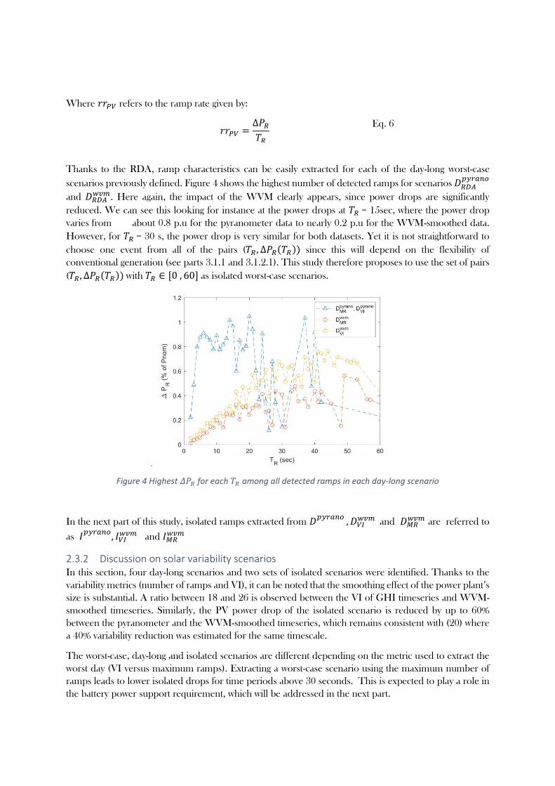
Thanks to the RDA, ramp characteristics can be easily extracted for each of the day-long worst-case

scenarios previously defined. Figure 4 shows the highest number of detected ramps for scenarios 𝐷𝑅𝐷𝐴𝑝𝑦𝑟𝑎𝑛𝑜

and 𝐷𝑅𝐷𝐴𝑤𝑣𝑚. Here again, the impact of the WVM clearly appears, since power drops are significantly

reduced. We can see this looking for instance at the power drops at 𝑇𝑅 = 15sec, where the power drop

varies from about 0.8 p.u for the pyranometer data to nearly 0.2 p.u for the WVM-smoothed data.

However, for 𝑇𝑅 = 30 s, the power drop is very similar for both datasets. Yet it is not straightforward to

choose one event from all of the pairs (𝑇𝑅 , Δ𝑃𝑅(𝑇𝑅)) since this will depend on the flexibility of

conventional generation (see parts 3.1.1 and 3.1.2.1). This study therefore proposes to use the set of pairs

(𝑇𝑅 , Δ𝑃𝑅(𝑇𝑅)) with 𝑇𝑅 ∈ [0 , 60] as isolated worst-case scenarios.

Figure 4 Highest 𝛥𝑃𝑅 for each 𝑇𝑅 among all detected ramps in each day-long scenario

In the next part of this study, isolated ramps extracted from 𝐷𝑝𝑦𝑟𝑎𝑛𝑜

, 𝐷𝑉𝐼𝑤𝑣𝑚 and 𝐷𝑀𝑅

𝑤𝑣𝑚 are referred to

as 𝐼𝑝𝑦𝑟𝑎𝑛𝑜

, 𝐼𝑉𝐼𝑤𝑣𝑚 and 𝐼𝑀𝑅

𝑤𝑣𝑚

2.3.2 Discussion on solar variability scenarios In this section, four day-long scenarios and two sets of isolated scenarios were identified. Thanks to the

variability metrics (number of ramps and VI), it can be noted that the smoothing effect of the power plant’s

size is substantial. A ratio between 18 and 26 is observed between the VI of GHI timeseries and WVM-

smoothed timeseries. Similarly, the PV power drop of the isolated scenario is reduced by up to 60%

between the pyranometer and the WVM-smoothed timeseries, which remains consistent with (20) where

a 40% variability reduction was estimated for the same timescale.

The worst-case, day-long and isolated scenarios are different depending on the metric used to extract the

worst day (VI versus maximum ramps). Extracting a worst-case scenario using the maximum number of

ramps leads to lower isolated drops for time periods above 30 seconds. This is expected to play a role in

the battery power support requirement, which will be addressed in the next part.

The isolated scenario extracted using the RDA shows ramp rates of between 2.25%/sec and 1.25%/sec

with a maximum 72% drop in nominal power within 42 seconds for the set 𝐼𝑉𝐼𝑤𝑣𝑚. This is a more

comprehensive way of characterizing solar variability than considering the entire timeseries since it reduces

it to a single drop event. However, the accuracy of the method needs to be proven by comparing the

batteries obtained in both day-long and isolated scenarios.

The next section will evaluate the battery power requirements for each of the six identified scenarios while

trying to determine the best way of addressing solar-PV variability.

3 Battery power capacity sizing It has been shown in the previous section that the variability scenario can be significantly altered by more

accurate modelling of the PV plant thanks to the WVM.

Similarly, a more detailed modelling of the power plant is expected to reduce the battery requirements for

off-grid systems. This section will evaluate the battery capacity needs for two variability scenarios and

compare the gain associated with an increase in model accuracy for the PV plant and the power system.

This will be compared with the gain obtained by smoothing out the solar variability as well as the

uncertainty introduced by the choice of variability scenarios.

3.1 Methodologies for hybrid sizing

3.1.1 Power adequacy battery sizing A comprehensive, effective methodology for determining battery capacity consists in detecting the

maximum power gap between the load and the generators. In (12), power adequacy battery sizing is used

to compensate solar ramps when generators have insufficient ramping capacity. Eq. 7 and Eq. 8 show how

the capacity is calculated while respecting the ramping constraint expressed by Eq. 9.

𝑃𝑢𝑛𝑚𝑒𝑡 𝑙𝑜𝑎𝑑(𝑡) = 𝑃𝐿 − 𝑃𝑓𝑜𝑠𝑠𝑖𝑙(𝑡) − 𝑃𝑃𝑉(𝑡) Eq. 7

𝐶𝑏𝑎𝑡 = 𝑚𝑎𝑥𝑡

(𝑃𝑢𝑛𝑚𝑒𝑡 𝑙𝑜𝑎𝑑(𝑡)) Eq. 8

𝑃𝑓𝑜𝑠𝑠𝑖𝑙 (𝑡 + 1) − 𝑃𝑓𝑜𝑠𝑠𝑖𝑙 (𝑡) < 𝑟𝑟𝑓𝑜𝑠𝑠𝑖𝑙 Eq. 9

Where 𝑃𝑃𝑉 is the PV power, 𝑃𝑓𝑜𝑠𝑠𝑖𝑙 is the power generated by fossil units, 𝑃𝐿 is the load demand and

𝑃𝑢𝑛𝑚𝑒𝑡 𝑙𝑜𝑎𝑑 is the amount of power that cannot be satisfied by the generating units. 𝐶𝑏𝑎𝑡 is the battery

power capacity obtained by filling the power gap 𝑃𝑢𝑛𝑚𝑒𝑡 𝑙𝑜𝑎𝑑 during the PV power loss.

The PV power 𝑃𝑃𝑉 is calculated from the PV plant’s rated capacity and GHI value. A large number of

advanced models exist to estimate PV plant performance based on optical and thermal simulation, such

as presented in (31), but require a detailed description of the power plant (module types, electrical layout,

etc.). In the context of variability analysis, the precise estimation of power absolute value is less important

than the power dynamics. Hence, a linear model is used in this study as shown in Eq. 10 (a constant value

of 0.97 is set for 𝜂𝑃𝑉𝑖𝑛𝑣).

𝑃𝑃𝑉(𝑡) =𝐺𝐻𝐼

1000𝑊/𝑚²∗ 𝑃𝑃𝑉

𝑟𝑎𝑡𝑒𝑑 ∗ 𝜂𝑃𝑉𝑖𝑛𝑣 Eq. 10

The main drawback of this methodology is the risk of capacity overestimation, as pointed out in (12,32).

The solution proposed by these papers was to allow ramp violation to prevent the sizing from being too

conservative. However, this method does not allow for fully robust sizing, as it can endanger the quality of

supply and even lead to electrical blackout for high renewable penetration rates.

3.1.2 Dynamic electrical modelling

3.1.2.1 Application of power system theory to hybrid systems As stated in the literature review, an increasing level of complexity is observed in battery sizing studies. As

a matter of fact, models with a low level of abstraction can evaluate power dynamics with more accuracy,

which may have the effect of reducing the battery power requirements during PV transients. Instead of

considering a perfect power equilibrium, dynamical studies aim to achieve power quality criteria at short

timescales thanks to primary reserves (fossil generators and battery systems) whilst ensuring the continuity

of load supply at longer timescales thanks to secondary and tertiary reserves (33). The role of energy

storage systems in the frequency regulation paradigm has been extensively studied for large systems (34)

as well as smaller isolated grids (35). In this study, only primary regulation is addressed.

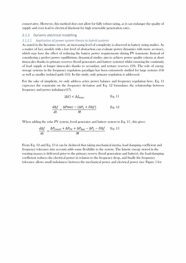
For the sake of simplicity, we only address active power balance and frequency regulation here. Eq. 11

expresses the constraint on the frequency deviation and Eq. 12 formulates the relationship between

frequency and power imbalance(17).

|Δ𝑓| < Δ𝑓𝑚𝑎𝑥 Eq. 11

𝑑Δ𝑓

𝑑𝑡=

Δ𝑃𝑚𝑒𝑐 − (Δ𝑃𝐿 + 𝐷Δ𝑓)

𝑀

Eq. 12

When adding the solar PV system, fossil generator and battery system to Eq. 13 , this gives:

𝑑Δ𝑓

𝑑𝑡 =

Δ𝑃𝑓𝑜𝑠𝑠𝑖𝑙 + Δ𝑃𝑃𝑉 + Δ𝑃𝑏𝑎𝑡 − Δ𝑃𝐿 − 𝐷Δ𝑓

𝑀

Eq. 13

From Eq. 12 and Eq. 13 it can be deduced that taking mechanical inertia, load damping coefficient and

frequency tolerance into account adds some flexibility to the system. The kinetic energy stored in the

rotating masses is delivered prior to the primary reserve (fossil generation and battery), the load-damping

coefficient reduces the electrical power in relation to the frequency drop, and finally the frequency

tolerance allows small imbalances between the mechanical power and electrical power (see Figure 5 for

graphical interpretation). This has the effect of reducing the primary reserve capacity requirement and

therefore the battery power capacity.

Figure 5 Evolution of frequency after a sudden load step (36).

3.1.2.2 Battery sizing procedure The frequency deviation can be simulated to evaluate the minimal battery capacity required to satisfy the

power quality criteria. This method is employed in several studies such as (37). Figure 6 shows the power

system model. PV and load profiles are injected as time-series in the model.

Figure 6 Power system and frequency regulation representation in the Laplacian domain

A proportional-integral derivative is used for the fossil generation contribution to frequency regulation

and is expressed in Eq. 14. The control signal 𝑃𝑓𝑜𝑠𝑠𝑖𝑙 ∗ then passes through ramping and power capacity

saturation blocks to obtain the power production 𝑃𝑓𝑜𝑠𝑠𝑖𝑙 .

𝑃𝑓𝑜𝑠𝑠𝑖𝑙 ∗ = 𝐾𝑝Δ𝑓 + 𝐾𝑖 ∫ Δ𝑓 + 𝐾𝑑

𝑑 Δ𝑓

𝑑𝑡 Eq. 14

An “energy-tank” model provides the storage dynamics as expressed in Eq. 17. Eq. 16 expresses the

inverter charging and discharging efficiencies, whilst Eq. 18 and Eq. 19 provide boundaries for energy

storage and power delivery. Values of 0.1 and 0.9 have been chosen for SOC boundaries similar to (38).

The final power 𝑃𝑏𝑎𝑡 delivered by the battery is integrated following Eq. 20.

𝑃𝑏𝑎𝑡∗ = 𝐾𝑏𝑎𝑡 ∗ Δ𝑓 Eq. 15

𝜂𝑆 =

1

𝜂𝑖𝑛𝑣𝜂𝑏𝑎𝑡 𝑖𝑓 𝑃𝑏𝑎𝑡

∗ < 0

𝜂𝑆 = 𝜂𝑖𝑛𝑣𝜂𝑏𝑎𝑡 𝑖𝑓 𝑃𝑏𝑎𝑡∗ ≥ 0

Eq. 16

𝐸𝑏𝑎𝑡(𝑡 + 1) = 𝐸𝑏𝑎𝑡(𝑡) + 𝜂𝑆𝑃𝑏𝑎𝑡∗ Δ𝑡 Eq. 17

𝑃𝑏𝑎𝑡𝑚𝑎𝑥 ≤ 𝑃𝑏𝑎𝑡

∗ ≤ 𝑃𝑏𝑎𝑡𝑚𝑖𝑛 Eq. 18

𝐸𝑏𝑎𝑡𝑚𝑎𝑥𝑆𝑂𝐶𝑚𝑖𝑛 ≤ 𝐸𝑏𝑎𝑡 ≤ 𝐸𝑏𝑎𝑡

𝑚𝑎𝑥𝑆𝑂𝐶𝑚𝑎𝑥 Eq. 19

𝑃𝑏𝑎𝑡 = Δ𝐸𝑏𝑎𝑡

𝛿𝑡 Eq. 20

Once the frequency timeseries has been simulated thanks to the dynamic model, an optimization method

is necessary to obtain the minimal battery capacity. Several methods may be used with varying levels of

complexity. For example, the authors in (39) implemented an analytic optimization with a fixed interval

and a particle swarm optimization procedure to reduce computational time. In this paper, a bisection

method is employed to evaluate the minimal battery requirements by running successive simulations and

varying storage capacity. This method can reduce the number of iterations as compared to fixed-interval

research. The searching interval is divided by 2 at each iteration until the final tolerance 𝜖 is reached. The

bisection method aims at minimizing the battery capacity 𝑃𝑏𝑎𝑡 by evaluating the power quality function

𝜈𝑃𝑏𝑎𝑡 defined by Eq. 21. Since 𝜈𝑋 is expected to monotonically decrease, more complex optimization

methods are not required to guarantee the convergence, although they may accelerate the solving time.

𝜈𝑋 = Δ𝑓𝑚𝑎𝑥 − min(𝛥𝑓𝑠𝑖𝑚 | 𝐶𝑏𝑎𝑡 = 𝑋) Eq. 21

Where 𝛥𝑓𝑠𝑖𝑚 is the frequency timeseries obtained by simulating the system with a battery power capacity

𝐶𝑏𝑎𝑡. The optimization procedure is shown in Annex. The searching interval is formed by [𝛼𝑖, β𝑖], while

𝛼0 and 𝛽0 are the lower and upper bounds for the optimization. The initial upper bound 𝛽0 = 𝐶0 is

given by the battery capacity calculated by the power adequacy method for the same scenario.

3.2 Conclusion on sizing methodologies Power adequacy and dynamic sizing procedures have been described previously in this section. Thanks

to the modelling of mechanical inertia and damping, as well as frequency shift tolerance, the battery

capacity requirement is expected to be lower for dynamic sizing than for power adequacy. This makes it

necessary to increase the level of complexity of sizing procedures and models. However, the scenarios

identified in section 2 show various levels of perturbation. The wrong choice of variability scenario may

eradicate the gains obtained by implementing a complex sizing strategy. In the next section, we employ

the six scenarios identified as input for both sizing methodologies and compare the resulting battery power

capacity. The overall process is shown in Figure 7.

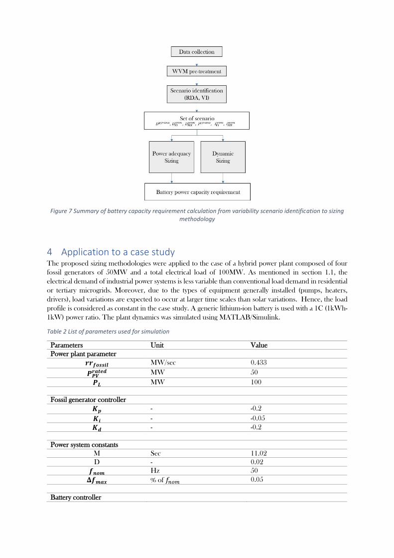
Figure 7 Summary of battery capacity requirement calculation from variability scenario identification to sizing methodology

4 Application to a case study The proposed sizing methodologies were applied to the case of a hybrid power plant composed of four

fossil generators of 50MW and a total electrical load of 100MW. As mentioned in section 1.1, the

electrical demand of industrial power systems is less variable than conventional load demand in residential

or tertiary microgrids. Moreover, due to the types of equipment generally installed (pumps, heaters,

drivers), load variations are expected to occur at larger time scales than solar variations. Hence, the load

profile is considered as constant in the case study. A generic lithium-ion battery is used with a 1C (1kWh-

1kW) power ratio. The plant dynamics was simulated using MATLAB/Simulink.

Table 2 List of parameters used for simulation

Parameters Unit Value

Power plant parameter

𝒓𝒓𝒇𝒐𝒔𝒔𝒊𝒍 MW/sec 0.433

𝑷𝑷𝑽𝒓𝒂𝒕𝒆𝒅 MW 50

𝑷𝑳 MW 100

Fossil generator controller

𝑲𝒑 - -0.2

𝑲𝒊 - -0.05

𝑲𝒅 - -0.2

Power system constants

M Sec 11.02

D - 0.02

𝒇𝒏𝒐𝒎 Hz 50

𝚫𝒇𝒎𝒂𝒙 % of 𝑓𝑛𝑜𝑚 0.05

Battery controller

𝑲𝒃𝒂𝒕 - 40

𝜼𝒊𝒏𝒗 - 0.98

𝜼𝒃𝒂𝒕 - 1

4.1.1 Power adequacy sizing The power adequacy sizing was applied to the scenarios presented in part 2.3.1. The set 𝐼𝑝𝑦𝑟𝑎𝑛𝑜 gave a

maximum power capacity requirement of 43.96MW which was found with the pair (𝑇𝑅 = 6𝑠, Δ𝑃𝑅 =0.93

p.u). The 𝐼𝑀𝑅𝑤𝑣𝑚 gave a power capacity requirement of 10.25 MW against 21.34 for 𝐼𝑉𝐼

𝑤𝑣𝑚 (see Table 3).

This results show that maximum battery capacity is not obtained with the same ramp duration, which

justifies the use of a whole set of ramps. The power dispatch is plotted in Figure 8 for two isolated

scenarios.

Table 3 Final battery capacity for isolated scenarios using power adequacy sizing

Set 𝑰𝒑𝒚𝒓𝒂𝒏𝒐 𝑰𝑴𝑹𝒘𝒗𝒎 𝑰𝑽𝑰

𝒘𝒗𝒎

Max battery power

requirement (MW)

43.96 10.25 21.34

Variability scenario

𝑻𝑹 (s) 6 24 29

𝚫𝑷𝑹 (p.u of Pnom) 0.93 0.41 0.67

Figure 8 Ramp events with the highest battery requirements from sets 𝐼𝑝𝑦𝑟𝑎𝑛𝑜 and 𝐼𝑀𝑅𝑤𝑣𝑚(method: power

adequacy sizing).

Results for day-long scenarios 𝐷𝑝𝑦𝑟𝑎𝑛𝑜

, 𝐷𝑀𝑅𝑤𝑣𝑚 and 𝐷𝑉𝐼

𝑤𝑣𝑚 give maximum battery power requirements of

44.7MW, 16.3MW and 25MW respectively.

4.1.2 Dynamic model sizing To initialize the first interval for the bisection method, the value 𝐶0 was set to the battery capacity found

in 4.1.1 for the same scenario. Figure 9 shows the power dispatch obtained with both the power adequacy

method and the dynamic simulation. The role of the frequency shift tolerance as a buffer clearly appears.

The battery peak power is reduced from 21.34MW to 15.23 MW with the dynamic model with a

frequency maintained above -0.05 p.u. This confirms the ability of the dynamical model to refine battery

requirements by taking the kinetic energy of rotors into account.

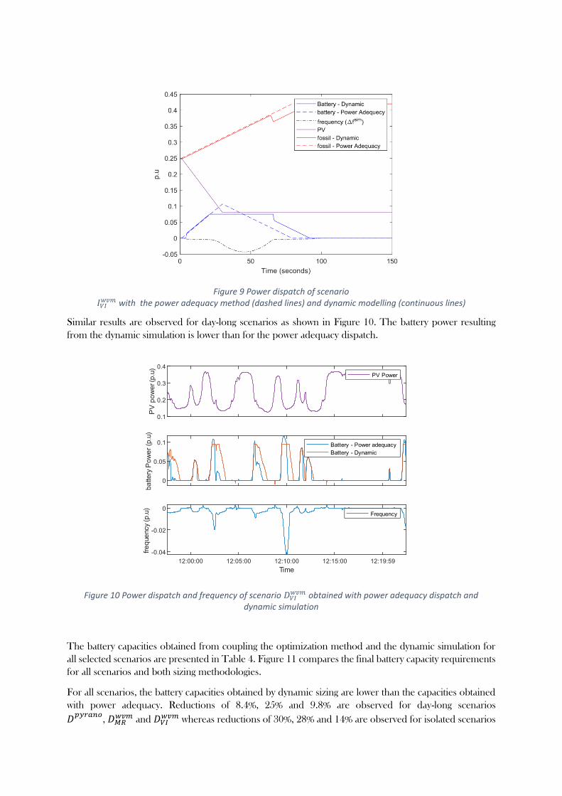
Figure 9 Power dispatch of scenario 𝐼𝑉𝐼

𝑤𝑣𝑚 with the power adequacy method (dashed lines) and dynamic modelling (continuous lines)

Similar results are observed for day-long scenarios as shown in Figure 10. The battery power resulting

from the dynamic simulation is lower than for the power adequacy dispatch.

Figure 10 Power dispatch and frequency of scenario 𝐷𝑉𝐼𝑤𝑣𝑚 obtained with power adequacy dispatch and

dynamic simulation

The battery capacities obtained from coupling the optimization method and the dynamic simulation for

all selected scenarios are presented in Table 4. Figure 11 compares the final battery capacity requirements

for all scenarios and both sizing methodologies.

For all scenarios, the battery capacities obtained by dynamic sizing are lower than the capacities obtained

with power adequacy. Reductions of 8.4%, 25% and 9.8% are observed for day-long scenarios

𝐷𝑝𝑦𝑟𝑎𝑛𝑜

, 𝐷𝑀𝑅𝑤𝑣𝑚 and 𝐷𝑉𝐼

𝑤𝑣𝑚 whereas reductions of 30%, 28% and 14% are observed for isolated scenarios

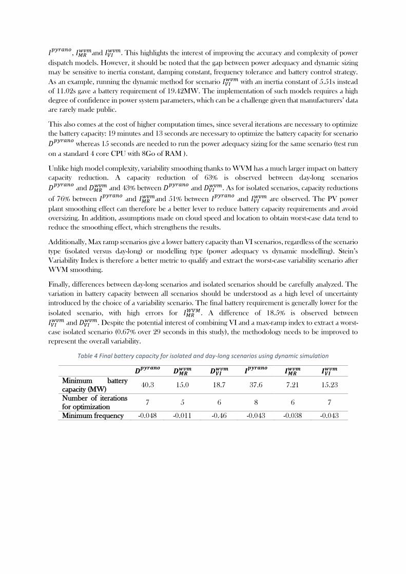
𝐼𝑝𝑦𝑟𝑎𝑛𝑜

, 𝐼𝑀𝑅𝑤𝑣𝑚and 𝐼𝑉𝐼

𝑤𝑣𝑚. This highlights the interest of improving the accuracy and complexity of power

dispatch models. However, it should be noted that the gap between power adequacy and dynamic sizing

may be sensitive to inertia constant, damping constant, frequency tolerance and battery control strategy.

As an example, running the dynamic method for scenario 𝐼𝑉𝐼𝑤𝑣𝑚 with an inertia constant of 5.51s instead

of 11.02s gave a battery requirement of 19.42MW. The implementation of such models requires a high

degree of confidence in power system parameters, which can be a challenge given that manufacturers’ data

are rarely made public.

This also comes at the cost of higher computation times, since several iterations are necessary to optimize

the battery capacity: 19 minutes and 13 seconds are necessary to optimize the battery capacity for scenario

𝐷𝑝𝑦𝑟𝑎𝑛𝑜

whereas 15 seconds are needed to run the power adequacy sizing for the same scenario (test run

on a standard 4 core CPU with 8Go of RAM ).

Unlike high model complexity, variability smoothing thanks to WVM has a much larger impact on battery

capacity reduction. A capacity reduction of 63% is observed between day-long scenarios

𝐷𝑝𝑦𝑟𝑎𝑛𝑜

and 𝐷𝑀𝑅𝑤𝑣𝑚 and 43% between 𝐷

𝑝𝑦𝑟𝑎𝑛𝑜 and 𝐷𝑉𝐼

𝑤𝑣𝑚. As for isolated scenarios, capacity reductions

of 76% between 𝐼𝑝𝑦𝑟𝑎𝑛𝑜

and 𝐼𝑀𝑅𝑤𝑣𝑚and 51% between 𝐼

𝑝𝑦𝑟𝑎𝑛𝑜 and 𝐼𝑉𝐼

𝑤𝑣𝑚 are observed. The PV power

plant smoothing effect can therefore be a better lever to reduce battery capacity requirements and avoid

oversizing. In addition, assumptions made on cloud speed and location to obtain worst-case data tend to

reduce the smoothing effect, which strengthens the results.

Additionally, Max ramp scenarios give a lower battery capacity than VI scenarios, regardless of the scenario

type (isolated versus day-long) or modelling type (power adequacy vs dynamic modelling). Stein’s

Variability Index is therefore a better metric to qualify and extract the worst-case variability scenario after

WVM smoothing.

Finally, differences between day-long scenarios and isolated scenarios should be carefully analyzed. The

variation in battery capacity between all scenarios should be understood as a high level of uncertainty

introduced by the choice of a variability scenario. The final battery requirement is generally lower for the

isolated scenario, with high errors for 𝐼𝑀𝑅𝑊𝑉𝑀. A difference of 18.5% is observed between

𝐼𝑉𝐼𝑤𝑣𝑚 and 𝐷𝑉𝐼

𝑤𝑣𝑚. Despite the potential interest of combining VI and a max-ramp index to extract a worst-

case isolated scenario (0.67% over 29 seconds in this study), the methodology needs to be improved to

represent the overall variability.

Table 4 Final battery capacity for isolated and day-long scenarios using dynamic simulation

𝑫𝒑𝒚𝒓𝒂𝒏𝒐

𝑫𝑴𝑹𝒘𝒗𝒎 𝑫𝑽𝑰

𝒘𝒗𝒎 𝑰𝒑𝒚𝒓𝒂𝒏𝒐

𝑰𝑴𝑹𝒘𝒗𝒎 𝑰𝑽𝑰

𝒘𝒗𝒎

Minimum battery

capacity (MW) 40.3 15.0 18.7 37.6 7.21 15.23

Number of iterations

for optimization 7 5 6 8 6 7

Minimum frequency -0.048 -0.011 -0.46 -0.043 -0.038 -0.043

Figure 11 Summary of battery power requirements for all selected scenarios (blue: dynamic modelling, red: power adequacy sizing)

4.1.3 Economic Analysis Bearing in mind the proposed microgrid configuration and the different battery solutions obtained after

applying the different methodologies, we present a basic economic analysis of the solutions, considering

two configurations:

• The first configuration (base case) is the fossil-based solution that provides a 100 MW power

supply during the 8,760 hours of the year.

• The second configuration considers the fossil-based power plant plus the 50 MWp solar

installation and a battery system with a capacity of 1C, with a size corresponding to that presented

in Table 4.

The approach is based in the analysis of the LCOE for both solutions, due to its acceptability in the

evaluation and a comparison of power plant configurations in different contexts (40). In this paper, the

following were considered: an inflation rate of 3%, a return rate of 7%, and a duration of 20 years for

computing the LCOE.

Table 5 shows the different values that were considered in the economic analysis for computing the fixed

and operational costs of the different components and fuel consumption. The information was extracted

from available documents and databases providing fuel prices (41) and microgrid components costs (42).

The chosen values allowed us to perform a relatively optimistic simulation in terms of battery prices, which

decrease considerably every year, whereas an average value for the gas price was considered, bearing in

mind the industrial contract that the plant operator might have for distribution.

Table 5 Selected prices for performing the economic analysis.

Interval

Selected

Value

Gas price ($ / kWh) 0.00 - 0.125 0.05

PV price ($ / kWp)* 0.50 - 1.10 0.88

PV OPEX ($ / MWp / yr) 250 - 1000 500

PV power degradation (% / yr) 0.1 – 1.0 0.5

Battery Price ($ / kWh) ** 350 – 600 495

Battery inverter ($ / kW)** 150 - 220 200

Battery system OPEX (% of CAPEX/yr) 0.1 - 0.5 0.5 *Includes Inverters, Cabling, Installation

**Includes Cabling, Installation

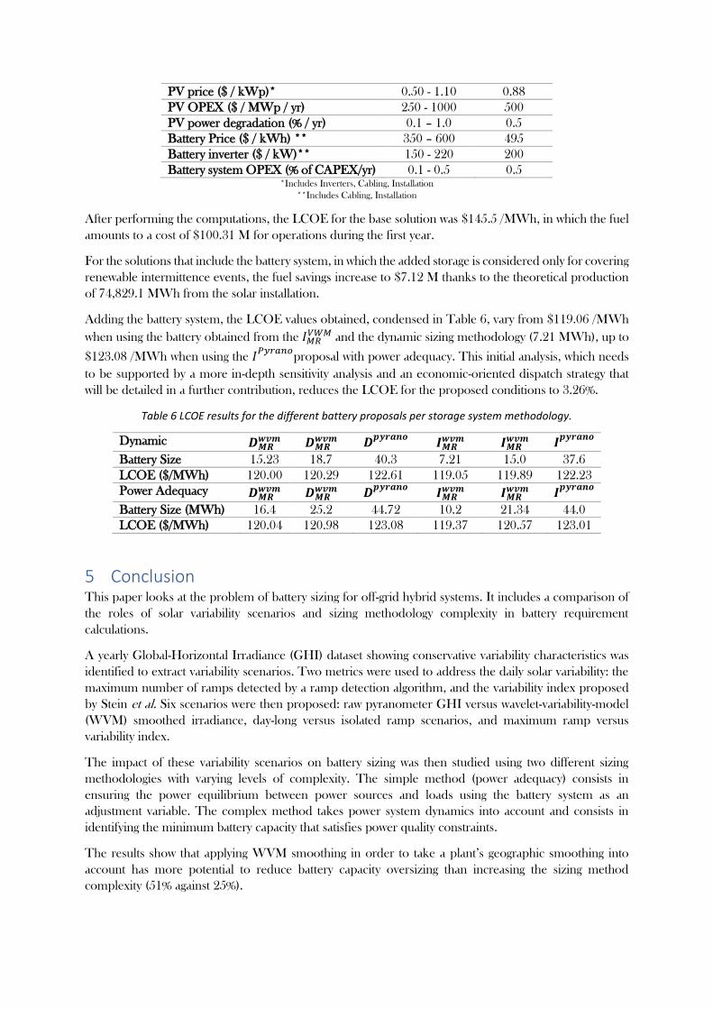
After performing the computations, the LCOE for the base solution was $145.5 /MWh, in which the fuel

amounts to a cost of $100.31 M for operations during the first year.

For the solutions that include the battery system, in which the added storage is considered only for covering

renewable intermittence events, the fuel savings increase to $7.12 M thanks to the theoretical production

of 74,829.1 MWh from the solar installation.

Adding the battery system, the LCOE values obtained, condensed in Table 6, vary from $119.06 /MWh

when using the battery obtained from the 𝐼𝑀𝑅𝑉𝑊𝑀 and the dynamic sizing methodology (7.21 MWh), up to

$123.08 /MWh when using the 𝐼𝑃𝑦𝑟𝑎𝑛𝑜

proposal with power adequacy. This initial analysis, which needs

to be supported by a more in-depth sensitivity analysis and an economic-oriented dispatch strategy that

will be detailed in a further contribution, reduces the LCOE for the proposed conditions to 3.26%.

Table 6 LCOE results for the different battery proposals per storage system methodology.

Dynamic 𝑫𝑴𝑹𝒘𝒗𝒎 𝑫𝑴𝑹

𝒘𝒗𝒎 𝑫𝒑𝒚𝒓𝒂𝒏𝒐

𝑰𝑴𝑹𝒘𝒗𝒎 𝑰𝑴𝑹

𝒘𝒗𝒎 𝑰𝒑𝒚𝒓𝒂𝒏𝒐

Battery Size 15.23 18.7 40.3 7.21 15.0 37.6

LCOE ($/MWh) 120.00 120.29 122.61 119.05 119.89 122.23

Power Adequacy 𝑫𝑴𝑹𝒘𝒗𝒎 𝑫𝑴𝑹

𝒘𝒗𝒎 𝑫𝒑𝒚𝒓𝒂𝒏𝒐

𝑰𝑴𝑹𝒘𝒗𝒎 𝑰𝑴𝑹

𝒘𝒗𝒎 𝑰𝒑𝒚𝒓𝒂𝒏𝒐

Battery Size (MWh) 16.4 25.2 44.72 10.2 21.34 44.0

LCOE ($/MWh) 120.04 120.98 123.08 119.37 120.57 123.01

5 Conclusion This paper looks at the problem of battery sizing for off-grid hybrid systems. It includes a comparison of

the roles of solar variability scenarios and sizing methodology complexity in battery requirement

calculations.

A yearly Global-Horizontal Irradiance (GHI) dataset showing conservative variability characteristics was

identified to extract variability scenarios. Two metrics were used to address the daily solar variability: the

maximum number of ramps detected by a ramp detection algorithm, and the variability index proposed

by Stein et al. Six scenarios were then proposed: raw pyranometer GHI versus wavelet-variability-model

(WVM) smoothed irradiance, day-long versus isolated ramp scenarios, and maximum ramp versus

variability index.

The impact of these variability scenarios on battery sizing was then studied using two different sizing

methodologies with varying levels of complexity. The simple method (power adequacy) consists in

ensuring the power equilibrium between power sources and loads using the battery system as an

adjustment variable. The complex method takes power system dynamics into account and consists in

identifying the minimum battery capacity that satisfies power quality constraints.

The results show that applying WVM smoothing in order to take a plant’s geographic smoothing into

account has more potential to reduce battery capacity oversizing than increasing the sizing method

complexity (51% against 25%).

This shows that the power plant smoothing effect and the proper variability scenario extracted are crucial

for estimating battery capacity and must not be neglected during hybrid power plant sizing. Neglecting the

power plant smoothing effect may lead to a significant over-estimation of the battery capacity, and therefore

higher electricity costs. On the other hand, a proper scenario identification method avoids battery under-

estimation and therefore prevents the degradation of power quality and grid reliability. This can be

illustrated by basic economic analysis of the hybrid solutions in which the battery system overestimation

will increase the levelized costs of electricity of the system, thus representing additional operational costs.

Lastly, the combination of VI and a ramp-detection algorithm to identify a worst-case isolated ramp

scenario led to an error of 18.5% as compared to the day-long simulation. One perspective to continue

with this work is to improve the isolated scenario generation to obtain a better match with worst-case day-

long scenarios and simplify battery sizing procedures.

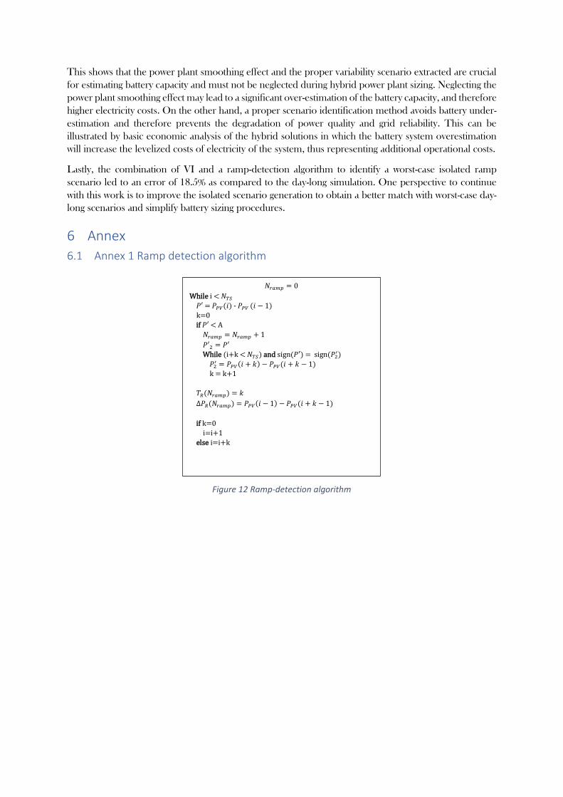
6 Annex

6.1 Annex 1 Ramp detection algorithm

Figure 12 Ramp-detection algorithm

𝑁𝑟𝑎𝑚𝑝 = 0

While i < 𝑁𝑇𝑆

𝑃′ = 𝑃𝑃𝑉(𝑖) - 𝑃𝑃𝑉 (𝑖 − 1)

k=0

if 𝑃′ < A

𝑁𝑟𝑎𝑚𝑝 = 𝑁𝑟𝑎𝑚𝑝 + 1

𝑃′2 = 𝑃′

While (i+k < 𝑁𝑇𝑆) and sign(𝑃′) = sign(𝑃2′)

𝑃2′ = 𝑃𝑃𝑉(𝑖 + 𝑘) − 𝑃𝑃𝑉(𝑖 + 𝑘 − 1)

k = k+1

𝑇𝑅(𝑁𝑟𝑎𝑚𝑝) = 𝑘

Δ𝑃𝑅(𝑁𝑟𝑎𝑚𝑝) = 𝑃𝑃𝑉(𝑖 − 1) − 𝑃𝑃𝑉(𝑖 + 𝑘 − 1)

if k=0

i=i+1

else i=i+k

6.2 Annex 2 Battery sizing optimization procedure

Figure 13 Battery optimization procedure

7 References

1. IEA. Tracking Industry [Internet]. Paris: IEA; 2019 May [cited 2019 Apr 23]. (Tracking report). Available from: https://www.iea.org/reports/tracking-industry

2. Alby P, Dethier J-J, Straub S. Firms Operating under Electricity Constraints in Developing Countries. The World Bank Economic Review. 2013;27(1):109–32.

3. Rissman J, Bataille C, Masanet E, Aden N, Morrow WR, Zhou N, et al. Technologies and policies to decarbonize global industry: Review and assessment of mitigation drivers through 2070. Applied Energy. 2020 May 15;266:114848.

4. Hamedani Golshan ME, Masoum MAS, Derakhshandeh SY. Profit-based unit commitment with security constraints and fair allocation of cost saving in industrial microgrids. IET Science, Measurement & Technology. 2013 Nov 1;7(6):315–25.

5. Soshinskaya M, Crijns-Graus WHJ, van der Meer J, Guerrero JM. Application of a microgrid with renewables for a water treatment plant. Applied Energy. 2014 Dec 1;134:20–34.

6. Riboldi L, Nord L. Offshore Power Plants Integrating a Wind Farm: Design Optimisation and Techno-Economic Assessment Based on Surrogate Modelling. Processes. 2018 Dec 4;6(12):249.

7. ARENA. Weipa solar farm - Australian Renewable Energy Agency (ARENA) [Internet]. Australian Renewable Energy Agency. [cited 2019 Apr 23]. Available from: https://arena.gov.au/projects/weipa-solar-farm/

8. Nosratabadi SM, Hooshmand R-A, Gholipour E, Rahimi S. Modeling and simulation of long term stochastic assessment in industrial microgrids proficiency considering renewable resources and load growth. Simulation Modelling Practice and Theory. 2017 Jun;75:77–95.

9. Subramanyam V, Jin T, Novoa C. Sizing a renewable microgrid for flow shop manufacturing using climate analytics. Journal of Cleaner Production. 2020 Apr 10;252:119829.

10. Kubik ML, Coker PJ, Barlow JF. Increasing thermal plant flexibility in a high renewables power system. Applied Energy. 2015 Sep;154:102–11.

11. Banjar-Nahor KM, Garbuio L, Debusschere V, Hadjsaid N, Pham T-T-H, Sinisuka N. Study on Renewable Penetration Limits in a Typical Indonesian Islanded Microgrid Considering the Impact of Variable Renewables Integration and the Empowering Flexibility on Grid Stability. In: 2018 IEEE PES Innovative Smart Grid Technologies Conference Europe (ISGT-Europe) [Internet]. Sarajevo, Bosnia and Herzegovina: IEEE; 2018 [cited 2019 Mar 7]. p. 1–6. Available from: https://ieeexplore.ieee.org/document/8571673/

12. Makibar A, Narvarte L, Lorenzo E. On the relation between battery size and PV power ramp rate limitation. Solar Energy. 2017 Jan 15;142:182–93.

13. Wilson M. Lazard’s Levelized Cost of Storage Analysis—Version 6.0. 2020;40.

14. Lian J, Zhang Y, Ma C, Yang Y, Chaima E. A review on recent sizing methodologies of hybrid renewable energy systems. Energy Conversion and Management. 2019 Nov 1;199:112027.

15. HOMER Energy. HOMER - Hybrid Renewable and Distributed Generation System Design Software [Internet]. [cited 2019 Mar 19]. Available from: https://www.homerenergy.com/

16. Mashayekh S, Stadler M, Cardoso G, Heleno M, Madathil SC, Nagarajan H, et al. Security-Constrained Design of Isolated Multi-Energy Microgrids. IEEE Trans Power Syst. 2018 May;33(3):2452–62.

17. Kundur PS. Power system stability and control. Indian edition. Balu NJ, Lauby MG, editors. Mc Graw Hill Education (India) Private Limited; 1994. 1176 p. (The EPRI power system engineering series).

18. Lauret P, Perez R, Mazorra Aguiar L, Tapachès E, Diagne HM, David M. Characterization of the intraday variability regime of solar irradiation of climatically distinct locations. Solar Energy. 2016 Feb 1;125:99–110.

19. Lappalainen K, Wang GC, Kleissl J. Estimation of the largest expected photovoltaic power ramp rates. Applied Energy. 2020 Nov 15;278:115636.

20. Mills A, Ahlstrom M, Brower M, Ellis A, George R, Hoff T, et al. Dark Shadows. IEEE Power and Energy Magazine. 2011 May;9(3):33–41.

21. Cormode D, Cronin AD, Richardson W, Lorenzo AT, Brooks AE, DellaGiustina DN. Comparing ramp rates from large and small PV systems, and selection of batteries for ramp rate control. In: 2013 IEEE 39th Photovoltaic Specialists Conference (PVSC) [Internet]. Tampa, FL, USA: IEEE; 2013 [cited 2019 Jul 18]. p. 1805–10. Available from: http://ieeexplore.ieee.org/document/6744493/

22. Lave M, Kleissl J, Stein JS. A Wavelet-Based Variability Model (WVM) for Solar PV Power Plants. IEEE Transactions on Sustainable Energy. 2013 Apr;4(2):501–9.

23. Hannan MA, Faisal M, Jern Ker P, Begum RA, Dong ZY, Zhang C. Review of optimal methods and algorithms for sizing energy storage systems to achieve decarbonization in microgrid applications. Renewable and Sustainable Energy Reviews. 2020 Oct 1;131:110022.

24. Anoune K, Bouya M, Astito A, Abdellah AB. Sizing methods and optimization techniques for PV-wind based hybrid renewable energy system: A review. Renewable and Sustainable Energy Reviews. 2018 Oct;93:652–73.

25. Jayashree S, Malarvizhi K. Methodologies for Optimal Sizing of Battery Energy Storage in Microgrids : A Comprehensive Review. In: 2020 International Conference on Computer Communication and Informatics (ICCCI). 2020. p. 1–5.

26. Lave M. Solar variability zones: Satellite-derived zones that represent high-frequency ground variability. Solar Energy. 2017;10.

27. Lave M, Reno MJ, Broderick RJ. Characterizing local high-frequency solar variability and its impact to distribution studies. Solar Energy. 2015 Aug 1;118:327–37.

28. Sengupta M, Andreas A. Oahu Solar Measurement Grid (1-Year Archive): 1-Second Solar Irradiance; Oahu, Hawaii (Data) [Internet]. 2010 [cited 2019 Mar 19]. Available from: http://www.osti.gov/servlets/purl/1052451/

29. Stein J, Hansen C, Reno MJ. The variability index: A new and novel metric for quantifying irradiance and PV output variability. Sandia National Laboratories; 2012.

30. Lappalainen K, Valkealahti S. Recognition and modelling of irradiance transitions caused by moving clouds. Solar Energy. 2015 Feb 1;112:55–67.

31. F. Holmgren W, W. Hansen C, A. Mikofski M. pvlib python: a python package for modeling solar energy systems. JOSS. 2018 Sep 7;3(29):884.

32. Jahromi AA, Majzoobi A, Khodaei A, Bahramirad S, Zhang L, Paaso A, et al. Battery Energy Storage Requirements for Mitigating PV Output Fluctuations. In: 2018 IEEE PES Innovative Smart Grid Technologies Conference Europe (ISGT-Europe). 2018. p. 1–5.

33. Farrokhabadi M, Cañizares CA, Simpson-Porco JW, Nasr E, Fan L, Mendoza-Araya PA, et al. Microgrid Stability Definitions, Analysis, and Examples. IEEE Transactions on Power Systems. 2020 Jan;35(1):13–29.

34. Greenwood DM, Lim KY, Patsios C, Lyons PF, Lim YS, Taylor PC. Frequency response services designed for energy storage. Applied Energy. 2017 Oct 1;203:115–27.

35. El-Bidairi KS, Nguyen HD, Mahmoud TS, Jayasinghe SDG, Guerrero JM. Optimal sizing of Battery Energy Storage Systems for dynamic frequency control in an islanded microgrid: A case study of Flinders Island, Australia. Energy. 2020 Mar 15;195:117059.

36. Fraisse J-L, Karsenti L. Raccordement de la production décentralisée aux réseaux de distribution - Conditions d’intégration. 2014;41.

37. Alves E, Sanchez S, Brandao D, Tedeschi E. Smart Load Management with Energy Storage for Power Quality Enhancement in Wind-Powered Oil and Gas Applications. Energies. 2019 Aug 2;12(15):2985.

38. Cominesi SR, Farina M, Giulioni L, Picasso B, Scattolini R. Two-layer predictive control of a micro-grid including stochastic energy sources. In: 2015 American Control Conference (ACC). 2015. p. 918–23.

39. Kerdphol T, Qudaih Y, Mitani Y. Battery energy storage system size optimization in microgrid using particle swarm optimization. In: IEEE PES Innovative Smart Grid Technologies, Europe. 2014. p. 1–6.

40. Pawel I. The Cost of Storage – How to Calculate the Levelized Cost of Stored Energy (LCOE) and Applications to Renewable Energy Generation. Energy Procedia. 2014 Jan 1;46:68–77.

41. Electricity prices around the world [Internet]. GlobalPetrolPrices.com. [cited 2021 Jun 30]. Available from: https://www.globalpetrolprices.com/electricity_prices/

42. IRENA. Utility-scale batteries – Innovation Landscape Brief [Internet]. 2019 p. 24. Available from: https://www.irena.org/-/media/Files/IRENA/Agency/Publication/2019/Sep/IRENA_Utility-scale-batteries_2019.pdf