On the Queue-Overflow Probability of Wireless Systems :

A New Approach Combining Large Deviations with

Lyapunov Functions

V. J. Venkataramanan and Xiaojun Lin

Center for Wireless Systems and Applications

School of Electrical and Computer Engineering,

Purdue University, West Lafayette, IN 47907, U.S.A.

Email: {vvenkat,linx}@ecn.purdue.edu.

Abstract

In this paper we study the problem of characterizing the queue-overflow probability of

wireless scheduling algorithms. In wireless networks operated under queue-length-based

wireless scheduling algorithms, there often exists a tight coupling between the service-rate

process, the system backlog process, the arrival process and the channel variations. Al-

though one can use sample-path large-deviation techniques to form an estimate of the

queue-overflow probability under a given offered load, the formulation leads to a multi-

dimensional calculus of variations problem that is often very difficult to solve. In this

paper, we present a new technique for addressing this complexity issue. Using ideas from

the Lyapunov function approach in control theory, this technique maps the complex multi-

dimensional calculus of variations problem to a one-dimensional calculus of variations prob-

lem, and the latter is often much easier to solve. Further, under appropriate conditions, we

1

show that when a scheduling algorithm minimizes the drift of the Lyapunov function, the

algorithm will be optimal in the sense that it maximizes the asymptotic decay-rate of the

probability that the Lyapunov function values exceed a given threshold. We believe that

these results can potentially be used to study the queue-overflow probability of a large class

of wireless scheduling algorithms.

1 Introduction

A wireless network may be modeled as a system of queues with time-varying service rates. The

variability in service rates is due to a number of factors. First, channel fading and mobility

can lead to variations in the link capacity even if the transmission power is fixed. Second, the

transmission power can vary over time according to the power control policy. Third, due to radio

interference, it is usually preferable to schedule only a subset of links to be active at each time,

and to alternate the subset of activated links over time. All of these factors lead to a variable

service rate at each link.

When we study the performance of any system that involves queues, the first question that we

can ask is whether the system is stable or not. Here, stability means that all queue backlog (or

equivalently, the delay experienced by the packets) remains finite. Conversely, we can ask the

question that, in order to maintain stability, what is the largest offered load that the system can

carry. For wireless networks, these questions have led to results on throughput-optimal scheduling

and routing algorithms for managing wireless network resources. Here, we use the term scheduling

in the broader sense, i.e., it can include various control mechanisms at the MAC/PHY layer, such

as link scheduling, power control, and adaptive coding/modulation. In addition, for multi-hop

wireless networks, the routing functionality determines the path that each packet traverses,

which also plays a key role in determining the capacity of the network. A scheduling and routing

algorithm is throughput-optimal if, for any offer load under which any other scheduling and

routing algorithm can stabilize the system, this algorithm can stabilize the system as well. For

2

example, one such throughput-optimal algorithm is the so-called “maximum-weight” and “back-

pressure” algorithm proposed in the seminal work by Tassiulas and Ephremides in [1]. This

algorithm chooses at each time, among all possible scheduling and routing decisions, the one

that maximizes the sum of the link rates weighted by the differential backlog. This algorithm

has been shown to be throughput-optimal, and it has been the basis for many other throughput-

optimal algorithms for both cellular and multihop wireless networks.

Once we know about stability, we are then tempted to ask further questions regarding the

distribution of queue length (or delay). For example, at a given offered load, what is the proba-

bility that the queue length at any link exceeds a given threshold (or, that the delay experienced

by a packet is greater than a given threshold)? Conversely, what is the largest offered load that

the system can support at a given queue-overflow or delay constraint? (In other words, what is

the effective capacity region of the system under such constraints?) Clearly, these question are

important for applications that require more stringent delay guarantees than just stability.

Such problems for characterizing the queue-overflow probability or delay-violation probability

in wireless networks can be difficult to solve. Here we draw a comparison to similar queueing

problems in wireline networks. In wireline networks, even though the exact queue distribution

can be difficult to obtain, there have been a large body of work, especially those using large-

deviation techniques, to obtain sharp estimates of the queue-overflow probability [2, 3, 4, 5, 6, 7].

Essentially, we can compute the asymptotic decay-rate with which the queue-overflow probability

approaches zero as the overflow threshold approaches infinity. We can then compare the queueing

performance of different systems by their corresponding asymptotic decay-rates, and we can ask

questions regarding the largest offered load subject to the constraint that the decay-rate must be

no smaller than a given threshold value. Most results along this line assume that the service rate

of the queue is fixed (i.e., time-invariant), and the packet arrival process is known. These results

enable us to define the notion of effective bandwidth of the arrival process based on its (known)

statistics [2,3,4,5,6,7], which can then be used to determine the traffic carrying capability of the

3

system at a given queue-overflow constraint. In contrast, in wireless networks, the service rate

is time-varying. If the service rate process is again known a priori, large-deviation techniques

can be used to compute the effective capacity of the service rate process [8,9], which is a notion

similar to the effective bandwidth of the arrival process. This effective capacity can again be used

to determine the traffic carrying capability of the system at a given constraint on the decay-

rate of the queue-overflow probability. Unfortunately, under many wireless resource-allocation

algorithms of interest, even the service rate process is unknown a priori. For example, for a

system operated under the throughput-optimal Tassiulas-Ephremides algorithm of [1], or any

queue-length based algorithms, the service rates depend on the queue length, which in turn

depend on the past history of the arrival process and the channel state. Hence, the statistics of

the service rate process is unknown a priori. In this case, even the computation of the asymptotic

decay-rate of the queue-overflow probability becomes a very difficult problem. For these systems,

although it is still possible to use sample-path large-deviation techniques to form an estimate of

the decay-rate of the queue-overflow probability [10,11,12], such a formulation leads to a multi-

dimensional calculus-of-variations problem. Due to the complex coupling between the service

rate, the queue length, the arrival process, and the channel state, this multi-dimensional calculus

of variations problem is known to be very difficult [10,11,12,13].

Motivated by the Lyapunov function approach for proving stability of complex systems, in this

paper we provide a technique that addresses the complexity of the multi-dimensional calculus-

of-variations problem that arises in sample-path large-deviation studies. In essense, through the

use of a Lyapunov function, we map the multi-dimensional calculus-of-variations problem into a

one-dimensional calculus-of-variations problem, and the latter is often much easier to solve. The

solution to the one-dimensional calculus-of-variations problem will then provide us with an lower-

bound estimate of the decay-rate of the queue-overflow probability, and consequently, a lower-

bound estimate of the effective capacity region of the system. For many practical applications,

the resulting effective capacity region is useful because the queue-overflow constraint is known

4

to be satisfied (in the large-deviation sense).

When this idea was first presented in our earlier work [14], we have assumed that a large-

deviation principle (LDP) holds for the queue backlog process. Unfortunately, for many wireless

systems, such an LDP by itself is often difficult to check. In this paper, we prove that, even

without assuming an LDP for the queue backlog process, our Lyapunov function approach will

provide a lower bound on the decay-rate of the queue-overflow probability. Further, we provide

a useful condition when this bound becomes tight. Specifically, we show that if the schedul-

ing and routing algorithm minimizes the drift of the Lyapunov function at each point of the

fluid sample path, then the bound obtained through the Lyapunov function approach is exactly

equal to the asymptotic decay-rate of the probability that the Lyapunov function value exceeds a

given threshold. When this happens, the algorithm is in fact optimal in maximizing the asymp-

totic decay-rate of the probability that the Lyapunov function value overflows. Note that many

throughput-optimal algorithms are derived by minimizing the drift of a corresponding Lyapunov

function. Hence, the above optimality condition is applicable to a large class of scheduling and

routing algorithms. For example, according to this result, the back-pressure algorithm [1] max-

imizes the asymptotic decay-rate of the probability that the sum of the squares of the queues

exceeds a given threshold. We also provide another example (which is a more general version

than the problems studied in existing work), and demonstrate how to use this approach to derive

the exact value of the asymptotic decay-rate of the queue-overflow probability, along with the

corresponding effective capacity region.

We believe that this marriage between sample-path large-deviations and Lyapunov functions

can develop into a powerful theory to characterize the queueing behavior of wireless systems

under sophisticated scheduling and routing algorithms. We can potentially lower the difficulty

level of the queueing problem to that of a stability problem. In other words, for any scheduling

and routing algorithm that is provably stable, which usually means that there exists a Lyapunov

function, we could then apply this theory and recover important properties of the corresponding

5

queueing performance.

In our prior work [15], we have also used Lyapunov functions to study the large-deviation

decay rate of the queue-overflow probability in the setting of a single cell in a cellular system.

Such setting is also studied in [13] using a different approach. This paper differs from [15] in

several aspects. Firstly, the results of this paper are established for a much larger class of wireless

networks (including multi-hop wireless networks), a much larger class of scheduling algorithms

(including, e.g., the back-pressure algorithm), and more general overflow metrics. In contrast,

the work in [15] focuses on a single cell model, the so-called α-algorithms and the max-queue

overflow metric. The emphasis there is to develop practical near-optimal scheduling algorithms

for that setting. Secondly, this paper provides a more thorough understanding of the Lyapunov

function approach than [15]. Specifically, in Proposition 3, we establish that the decay-rate of

the stationary over-flow probability is bounded by the minimum-cost-to-overflow. For this result

to hold, we only assume that the system has a Lyapunov function that satisfies Assumptions

1 and 2. In contrast, the technique in [15] uses additional structure of the system. Similarly,

in Proposition 8, we state the condition under which the scheduling algorithm is optimal. This

condition is again ony related to the Lyapunov functions and hence is more general than the result

in [15]. Lastly, in [15], since the focus is more on the practical aspect, we have not included the

detailed proof of the Freidlin-Wentzell construction. In this paper, we provide the proof (See

Propositions 3 and 4), again under very general conditions.

The rest of the paper is organized as follows. We present the network model in Section 2. In

Section 3, we provide a general lower bound for the asymptotic decay-rate of the queue-overflow

probability using sample-path large-deviation theory. However, this bound involves a difficult

multi-dimensional calculus-of-variations problem. Then, in Section 4, we provide a Lyapunov

function based approach to address the complexity issue, which provides an even simpler lower

bound on the asymptotic decay-rate of the queue-overflow probability. In Section 5, we provide

a condition under which this lower bound is tight. In Section 6, we provide examples to show

6

how such an approach can be applied to various network settings. Then we conclude.

Throughout the paper, we use x to denote real numbers and ~x to denote vectors. For con-

venience, when we refer to a vector-valued stochastic process ~x(t) over a certain time-interval,

we often drop the index t and denote it by a bold-face symbol x. In other words, ~x(t) denotes

the value of the stochastic process x at time t. Unless stated otherwise, we use right derivatives

throughout this paper, i.e., ddt

x(t) = limδ↓0+

x(t+δ)−x(t)δ

.

2 The System Model

We assume the following model for a wireless system with N nodes and L links.

2.1 The Channel

We assume that time is divided into time-slots of unit length. In order to model channel fading,

we assume that at any time-slot t the state of the wireless channel, denoted by C(t), can be in

one of S (channel) states j = 1, 2, ..., S. We assume that the channel states C(t), t = 1, 2, ... are

i.i.d. across time. Let pj = P[C(t) = j], j = 1, 2, ..., S. and ~p = [p1, ..., pS].

For a fixed B, define the scaled channel state process on the time interval [−T, 0] as

sBj (t) =

1

B

B(T+t)∑

τ=0

1{C(τ)=j}, (1)

for t = mB−T , m = 0, ..., BT , and by linear interpolation otherwise. The parameter B is a scaling

factor that scales in time and magnitude. To see this, note that (1) is of the form 1B

f(B(T + t)).

The quantity sBj (t) can be interpreted as the sum of the (scaled) time in [−T, t] that the system

is at channel state j. Further, it is easy to check that∑S

j=1 sBj (t) = t + T for all t ∈ [−T, 0]. Let

~sB(t) = [sB1 (t), ...sB

S (t)]. Further, let φBj (t) = d

dtsB

j (t). (Note again that we use right-derivatives,

and that the right-derivative of sBj (t) is well defined almost everywhere on [−T, 0] except when

t = m/B − T for some integer m.) Let ~φB(t) = [φB1 (t), ..., φB

S (t)]. Note that∑S

j=1 φBj (t) = 1 for

almost all t ∈ [−T, 0].

7

We will soon see that the scaled channel state process satisfies a large-deviation principle

(LDP). For any ~φ = [φj, j = 1, ..., S] ≥ 0 and∑S

j=1 φj = 1, define H(~φ||~p) =∑S

j=1 φj logφj

pj.

(Here we use the convention that 0 log 0 = 0.) Let Φs[−T, 0] denote the space of functions ~s(t)

on [−T, 0] that satisfy the following condition: ~s(t) is component-wise non-decreasing on [−T, 0],

~s(−T ) = 0, and∑S

j=1 sj(t) = t + T for all t. Let this space be equipped with the essential

supremum norm [16, p176,p352], denoted here by || · ||T∞ . The sequence of scaled channel-

state processes sB = (~sB(t), t ∈ [−T, 0]) are known to satisfy a sample-path large deviation

principle [16, p176] with large-deviation rate-function ITs (s) given as follows:

ITs (s) =

∫ 0

−T

H

(

d

dt~s(t)||~p

)

dt,

if s ∈ Φs[−T, 0] is absolute continuous. (Note that ddt

~s(t) is well defined almost everywhere on

[−T, 0] when s = (~s(t), t ∈ [−T, 0]) is absolute continuous.) Otherwise,

ITs (s) = +∞.

Such a large-deviation principle means that, for any set Γ of trajectories in Φs[−T, 0], the prob-

ability that the sequence of scaled channel state processes sB fall into Γ must satisfy

− infs∈Γo

ITs (s) ≤ lim inf

B→∞

1

Blog P[sB ∈ Γ] (2)

≤ lim supB→∞

1

Blog P[sB ∈ Γ] ≤ − inf

s∈ΓITs (s),

where Γo and Γ denote the interior and closure, respectively, of the set Γ. In addition, if Γ is a

continuity set [16, p5], equality is achieved and we then have,

limB→∞

1

Blog P[sB ∈ Γ] = − inf

s∈ΓITs (s). (3)

Remark: The large-deviation rate-function ITs (·) characterizes how rare the occurrence of each

trajectory is. Note that ITs (s) ≥ 0 for all trajectory s. The larger the value of IT

s (s) is, the

further the “empirical probability distribution” ddt

~s(t) deviates from the underlying probability

distribution ~p. Hence, it is less likely that trajectory s will occur. Equation (3) reflects the

8

well-known large-deviation philosophy that “rare events occur in the most-likely way.” Precisely,

when B is large, the probability that the scaled channel-state process sB falls into a set Γ is

determined by the trajectory in Γ that is most likely to occur, i.e., with the smallest ITs (s).

2.2 The Arrival

The system serves packets from multiple classes k = 1, ..., K. Each class k corresponds to a

set Dk of destination nodes. In other words, once the class-k packets arrive at any node in Dk,

they will leave the system. Let Aki (t) denote the number of class-k packets arriving at node i at

time-slot t. We assume that [Aki (t)] is i.i.d. across time∗, and independent across arriving nodes

and across classes. In addition, we assume that Aki (t) is bounded by M for all i, k and t. Let

λki = E[Ak

i (t)].

The above arrival process also satisfies a well-known sample-path LDP as follows. Similar to

(1), define the scaled arrival process as,

ak,Bi (t) =

1

B

B(T+t)∑

τ=0

Aki (τ) (4)

for t = mB− T , m = 0, ..., BT , and by linear interpolation otherwise. Let ~aB(t) = [ak,B

i (t), i =

1, ..., N, k = 1, ..., K] and ~fB(t) = ddt~aB(t).

Define

Lki (f) = sup

θ

(

θf − log E[exp(θAki (0)]

)

.

For any ~f = [fki , i = 1, ..., N, k = 1, ..., K], let L(~f) =

∑Ni=1

∑Kk=1 Lk

i (fki ). Further, let Φa[−T, 0]

be the space of component-wise non-decreasing functions ~a(t) on [−T, 0] with ~a(−T ) = 0. Let

this space also be equipped with the essential supremum norm [16, p176,p352], denoted here

by || · ||T∞. Since the arrivals [Aki (t)] are i.i.d. in time, the sequence of scaled arrival-processes

aB = (~aB(t), t ∈ [−T, 0]) also satisfies a sample-path large-deviation principle [16, p176] with

∗The results of this paper can also be generalized to the case with time-correlated arrivals under suitable

conditions [4]. The key requirement is that the arrivals satify a large deviations principle.

9

large-deviation rate-function ITa (a) given as follows:

ITa (a) =

∫ 0

−T

L

(

d

dt~a(t)

)

dt,

if a ∈ Φa[−T, 0] is absolute continuous. (Note that ddt~a(t) is well-defined almost everywhere on

[−T, 0] when a = (~a(t), t ∈ [−T, 0]) is absolute continuous.) Otherwise,

ITa (a) = +∞.

A similar interpretation as in Equations (2) and (3) holds for ITa (·) as well, where the set Γ, in

this case is chosen from the space Φa[−T, 0].

2.3 The Queue

Let Xki (t) denote the backlog of class-k packets at node i at time t, and let ~X(t) = [Xk

i (t), i =

1, ..., N, k = 1, ..., K]. Let b(l) and e(l) denote the source-node and end-node, respectively, of

link l. Each link l then corresponds to a server with time-varying service rate, which serves

packets at node b(l) and transfers them to node e(l). The service offered by link l is determined

by the scheduling and routing algorithm. In general, this service rate may depend on the global

system backlog and the global channel state, and hence may correlate with the service at other

links/nodes. Let Ekl (j, ~X) denote the service offered by link l to class-k packets at node b(l), when

the state of the system is j and the global backlog is ~X. We impose the additional constraint

that Ekl (j, ~X) ≤ Xk

b(l). (In other words, the service offered by link l to class-k packets is no

greater than the backlog of class-k packets at the source node b(l).) By definition of Dk (the set

of destination nodes of class-k), Xki (t) = 0 for all nodes i ∈ Dk. For a node i not in Dk, the

evolution of the class-k backlog is given by

Xki (t + 1) = Xk

i (t) + Aki (t)

−S∑

j=1

1{C(t)=j}

L∑

l=1

RilEkl (j, ~X(t)), (5)

10

for all nodes i /∈ Dk, where Ril denote the connectivity matrix, i.e.,

Ril =

1, if i = b(l)

−1, if i = e(l)

0, otherwise.

Let El(j, ~X) =∑K

k=1Ekl (j, ~X), which denotes the aggregate service offered by link l. We assume

that, for each state j, the service-rate vector [El(j, ~X), l = 1, ..., L] must belong to a set Ej of

feasible service-rate vectors. We assume that for all j, the convex hull of Ej, denoted Conv(Ej),

is closed and bounded, and contains the intersection of a neighborhood of the origin and the

positive quadrant.

2.4 The Performance Measure

Assume that the offered load ~λ = [λki , i = 1, ..., N, k = 1, .., K] is such that the system is

stationary and ergodic (in Section 3.2 we will introduce conditions on the Lyapunov function

that imply this stability). In this paper, we will focus on the stationary probability that some

chosen norm of the system backlog exceeds a certain threshold B. In particular, let ǫ denote our

target value of the overflow probability, we would like to ensure that

P[|| ~X(0)|| ≥ B] ≤ ǫ, (6)

where || · || is an appropriately chosen norm, and B is the overflow threshold. Unfortunately, the

problem of calculating the exact probability P[|| ~X(0)|| ≥ B] is often mathematically intractable.

Instead, we will be interested in the decay rate of the queue-overflow probability, which is defined

by

I0(~λ) , − limB→∞

1

Blog P[|| ~X(0)|| ≥ B], (7)

whenever the limit on the right-hand-side exists. Note that if (7) holds, then when B is large,

the overflow probability can be approximated by

P[|| ~X(0)|| ≥ B] ≈ exp(−BI0(~λ)).

11

Hence, we refer to I0(~λ) as the asymptotic decay-rate of the queue-overflow probability. Using

the above approximation, in order to (approximately) satisfy the constraint (6), we only need to

ensure that

I0(~λ) ≥ θ , −log ǫ

B. (8)

We can then define the effective capacity region as the set of arrival rates ~λ such that the above

inequality holds. In more general settings, the limit in (7) may not exist or may not be easily

computed. Still, we may be able to find a lower bound I ′0(

~λ) of the decay-rate of the overflow

probability such that

lim supB→∞

1

Blog P[|| ~X(0)|| ≥ B] ≤ −I ′

0(~λ). (9)

Then exp(−BI ′0(

~λ)) provides an (approximate) upper bound on the overflow probability P[|| ~X(0)|| ≥

B], and we can find a lower bound on the effective capacity region as the set of ~λ such that

I ′0(

~λ) ≥ θ , − log ǫB

. In this paper, our goal is to provide effective techniques to estimate I0(~λ)

and/or I ′0(

~λ).

2.5 Examples

Before we proceed, we provide a few examples to clarify the above system model.

2.5.1 Example 1: cellular or access-point based networks

Consider a single cell in a cellular network or an access-point based network. Each user com-

municates directly with the basestation. Further, only one user can be selected for service at a

time. Let us focus on the downlink from the basestation to the users (the uplink can be treated

analogously). Since this is a single-hop model, we identify each link l with a particular user/class,

and hence we can drop the index k for traffic class. In other words, we use Al(t) to denote the

packets generated for the user associated with link l at time slot t, and use Xl(t) to denote the

backlog of link l at time t. Let El(j, ~X) be the service offered to link l when the channel state is

j and the global backlog is ~X = [Xl, l = 1, ..., L]. Imposing the constraint that El(j, ~X) ≤ Xl,

12

the evolution of the queue-length is then given by

Xl(t + 1) = Xl(t) + Al(t) −S∑

j=1

1{C(t)=j}El(j, ~X(t)). (10)

Note that this equation is a simplified version of (5).

When the channel state is j, let rlj denote the capacity of link l if it is selected for transmission.

Then for each state j the service-rate vector [El(j, ~X), l = 1, ..., L] must belong to the set Ej given

by

Ej = {[tlrlj, l = 1, ..., L] : tl ∈ [0, 1]

for all l, and only one element of [tl] is non-zero}.

A Queue-Length-Based Scheduling Policy: One important class of policies for choosing

El(j, ~X) (often referred to as the max-weight policy in the literature [17, 1]), is to serve the link

l such that the weighted queue-length rljXl is the largest among all users (ties can be broken

arbitrarily). Let l∗ = argmaxl rljXl. The policy can then be written as:

El(j, ~X) =

min{rlj, Xl}, if l = l∗

0, otherwise,

It is well-known that this class of policies are throughput-optimal, i.e., they can stabilize the

system under the largest set of offered loads [17].

Remark: When the arrivals Al(t) are constant, i.e., Al(t) = λl for all t, the constraint in (6)

becomes equivalent to a constraint on the delay-violation probability. To see this, assume that

new packets always arrive at the begining of a time-slot, and define the delay of a packet as

the number of time-slots until it is completely served†. Let Dl(t) denote the delay experienced

by the last packet that arrives at time slot t. If we use the convention that Xl(t) denotes the

queue-length for link l at the begining of time slot t (before arrivals have occurred), then for any

†When the service rates are real numbers, we implicitly assume that the packet can be divided into arbitrarily

small elements, and these elements can be served over multiple time-slots.

13

delay bound dl, we have

Dl(0) ≥ dl

⇐⇒ Cumulative service over time [0, dl − 1] < Xl(0) + λl

⇐⇒

dl−1∑

t=0

S∑

j=1

1{C(t)=j}El(j, ~X(t)) < Xl(0) + λl

⇐⇒ Xl(dl) > λl(dl − 1).

Hence, the two types of constraints are related by (see [9, 11])

P[Dl(0) ≥ dl] = P[Xl(dl) > λl(dl − 1)]

= P[Xl(0) > λl(dl − 1)],

where the last equality follows from the stationary assumption.

2.5.2 Example 2: Multihop Ad Hoc Wireless Networks

The full model described earlier in this section is most suitable for multihop wireless networks,

where Xki (t) represents the backlog of class-k packets at node i at time t, and its evolution is

given by (5). Unlike in Example 1 where only one user/link can be selected at each time, in multi-

hop wireless networks it is often possible to activate multiple links simultaneously. However, the

activated links must satisfy certain interference constraints, and their rates depend on the power

and interference levels. As a result, the set of feasible service-rate vectors often becomes more

complicated to describe than Example 1. We give two cases.

Case 1: Assume that the scheduling policy can decide whether to activate or inactivate a link,

but cannot change the transmission power of a link. Let πl = 1 if link l is activated, and πl = 0,

otherwise. Let ~π = [πl, l = 1, ..., L], and let Π denote the set of feasible activation vectors ~π.

Let rlj(~π) denote the rate of link l if the activation vector ~π is applied at state j. Then at each

channel state j, The set Ej of feasible service-rate vectors can be written as:

Ej = {[rlj, l = 1, ..., L] : there exists ~π ∈ Π

such that rlj ≤ rlj(~π) for all links l}. (11)

14

Case 2: Assume that the scheduling policy can decide both the activation pattern and the

power assignments. Let πl denote the power assignment of link l. πl = 0 if the link is not

activated. Let ~π = [πl, l = 1, ..., L], and let Π denote the set of feasible power-assignment

vectors ~π. Then at each channel state j, each vector ~π can again be mapped to a rate-vector

[rlj(~π), l = 1, ..., L]. The set Ej of feasible service-rate vectors can also be written as in (11).

A Queue-Length-Based Scheduling and Routing Algorithm: For both cases, the

scheduling and routing algorithm proposed in [1] (which is often referred to as the “back-pressure”

algorithm) is known to be throughput-optimal. At each time-slot t, for each link l, first find the

class k∗l (t) with the maximum differential backlog, i.e.,

k∗l (t) = argmax

k(Xk

b(l)(t) − Xke(l)(t)).

Let the corresponding differential backlog be

wl(t) = max{0, Xk∗

l(t)

b(l) (t) − Xk∗

l(t)

e(l) (t)}.

Then, when the channel state at time t is j, compute the schedule ~π∗j (t) that maximizes the sum

of the rates weighted by wl(t), i.e.,

~π∗j (t) = argmax

~π∈Π

wl(t)rlj(~π).

The scheduling and routing decision is then given by the following: if the channel state at

time-slot t is j,

• Scheduling: use the activation vector ~π∗j (t).

• Routing: on each link l, only serve the packets belonging to class k∗l (t).

In other words, the service rate vector is given by

Ekl (j, ~X) =

min{Xkb(l)(t), rlj(~π

∗j (t))}, if k = k∗

l (t)

0 otherwise.

15

3 A General Lower Bound on the Decay-Rate of the Queue-

Overflow Probability

In this section, we first provide a lower bound I ′0(

~λ) on the decay-rate of the queue-overflow

probability as defined in (9). Prior work [10,11] has derived the decay-rate of the queue-overflow

probability as the cost of the most-likely-path to overflow. The approach there requires that the

limiting mapping from the scaled channel-state process to the scaled queue-backlog process, to

be defined later, is unique and continuous with respect to a suitably chosen topological space, so

that the contraction principle [16, p131] can be invoked to establish a sample-path LDP for the

queue-backlog process. However, for general wireless systems, the mapping from the channel-

state process to the queue-backlog process may not be continuous, and hence the approach

in [10, 11] can not be applied. Nonetheless, in this section we show that, for a large class of

wireless systems, the cost of the most-likely-path to overflow is a lower bound of the decay-rate

of the queue-overflow probability. Recall that such a lower bound implies that we can then use

exp(−BI ′0(

~λ)) as an (approximate) upper bound on the overflow probability P[|| ~X(0)|| ≥ B].

Similar to the large-deviation scaling used in Section 2.1 and Section 2.2, define the scaled

backlog process as,

xk,Bi (t) =

1

BXk

i (B(T + t)), (12)

for t = mB− T , m = 0, ..., BT , and by linear interpolation otherwise. Let ~xB(t) = [xk,B

i (t), i =

1, ..., N, k = 1, ..., K]. The lower bound I ′0(

~λ) in (9) can then be written as

lim supB→∞

1

Blog P[||~xB(0)|| ≥ 1] ≤ −I ′

0(~λ). (13)

Before we proceed, we need to define the notion of a Fluid Sample Path (FSP). Note that

according to (5), given an initial condition on ~xB(−T ), the scaled backlog process xB = (~xB(t), t ∈

[−T, 0]) is related to the scaled channel-state process sB = (~sB(t), t ∈ [−T, 0]) and the scaled

16

arrival process aB = (~aB(t), t ∈ [−T, 0]) by

xk,Bi (t + 1/B) − xk,B

i (t)

1/B(14)

=

[

ak,Bi (t) − ak,B

i (t − 1B

)

1/B

]

−S∑

j=1

L∑

l=1

RilEkl (j, B~xB(t))

[

sBj (t) − sB

j (t − 1B

)

1/B

]

,

for i /∈ Dk, t = mB− T , m = 0, ..., BT and by linear interpolation otherwise. Thus, given any

T and any initial condition ~xB(−T ), Equation (14) defines a mapping from the scaled channel-

state process sB and the scaled arrival process aB to the scaled backlog process xB over the

time-interval [−T, 0]. As B → ∞, take any sequence of sB and aB (which may come from

different sample paths). They map to a sequence of scaled backlog processes xB. Note that

sB, aB and xB are all Lipschitz-continuous. Hence, for any such sequence (sB, aB,xB), there

must exist a subsequence that converges to a limiting process (s, a,x) uniformly over compact

intervals. We define any such limiting process as a Fluid Sample Path, or an FSP, which we

denote as (s, a,x)T , where the subscript denotes the starting time −T . Such an FSP often

satisfies the following differential equation obtained by letting B → ∞ on Equation (14):

d

dtxk

i (t) =d

dtak

i (t) −S∑

j=1

d

dtsj(t)

L∑

l=1

Rilekl (j, ~x(t)). (15)

where ekl (j, ~x(t)) is some appropriately-chosen limiting value of Ek

l (j, B~xB(t)). In the rest of the

paper, we sometimes denote FSPs as (s, a,x), i.e., without the time subscript T . In doing so,

we mean that there is some finite time T such that (s, a,x)T is an FSP.

Let

I ′0(

~λ) =

infT≥0,s,a,x

∫ 0

−T

[

H

(

d

dt~s(t)||~p

)

+ L

(

d

dt~a(t)

)]

dt

subject to (s, a,x)T is an FSP

~x(−T ) = 0, ||~x(0)|| ≥ 1. (16)

17

Our goal in this section to establish that I ′0(

~λ) defined in (16) satisfies (13), i.e., it is a lower-

bound on the decay rate of the queue-overflow probability. The FSP that attains the infimum,

on the right-hand-side of (16) (if such an FSP exists) is usually called the “most-likely path to

overflow.” Hence, this result (to be proved soon) states that the cost of the most-likely path to

overflow is a lower bound on the decay-rate of the queue-overflow probability. We will derive the

result in two steps. First, we consider a system that starts at time 0, and derive a lower bound

in Section 3.1 on the decay rate of the overflow probability at time BT . Then, we let T → ∞

and derive a lower bound on the decay-rate of the stationary overflow probability in Section 3.3.

3.1 Bounds for a Finite Time System

As a step towards proving the result on the stationary overflow probability, we first consider the

probability of overflow at time BT , P(|| ~X(BT )|| ≥ B), for a system that starts from ~X(0) = 0.

Note that according to the transformation ~xB(t) = 1B

~X(B(T + t)), we have ~xB(−T ) = 0 and

||~xB(0)|| ≥ 1. Let PB,T0 denote the probability distribution conditioned on ~xB(−T ) = 0. We

have the following bound on the probability of overflow.

Proposition 1 Fix T > 0. The following holds,

lim supB→∞

1

Blog PB,T

0 [||~xB(0)|| ≥ 1]

≤ − infs,a,x

∫ 0

−T

[

H

(

d

dt~s(t)||~p

)

+ L

(

d

dt~a(t)

)]

dt

subject to (s, a,x)T is an FSP

~x(−T ) = 0 and ||~x(0)|| ≥ 1. (17)

Instead of proving Proposition 1, we will prove a generalized version in Proposition 2. The

extra effort will serve useful in proving the stationary overflow case.

Fix ~x0. For the more general version, consider a system that starts with ~X(0) = B~x0 at time 0

(i.e., ~xB(−T ) = ~x0). Let PB,T~x0

denote the probability distribution conditioned on ~xB(−T ) = ~x0.

Let Φx[−T, 0] denote the space of non-negative Lipschitz-continuous functions on the interval

18

[−T, 0], equipped with the essential supremum norm. We can then show the following result,

which is comparable to Theorem 7.1 of [13] for a refined LDP.

Proposition 2 Fix T > 0. Let X denote a closed set in ℜNK. Let Γ denote a closed set of

trajectories x = (~x(t), t ∈ [−T, 0]) from the topological space Φx[−T, 0] that satisfies ~x(−T ) ∈ X .

The following holds,

lim supB→∞

1

Blog sup

~x0∈X

PB,T~x0

[xB ∈ Γ]

≤ − infs,a,x

∫ 0

−T

[

H

(

d

dt~s(t)||~p

)

+ L

(

d

dt~a(t)

)]

dt

subject to (s, a,x)T is an FSP

x ∈ Γ. (18)

Proof: Note that xB is related to sB and aB according to Equation (14). Let ΓB denote the set

of (sB, aB) on the interval [−T, 0] such that there exists ~x0 ∈ X with which (sB, aB) maps to a

backlog process xB that starts from ~xB(−T ) = ~x0 and satisfies xB ∈ Γ. Then for every ~x0 ∈ X ,

PB,T~x0

[xB ∈ Γ] ≤ P[(sB, aB) ∈ ΓB].

Note that the right-hand-side does not depend on ~x0. Further, for any fixed n, ΓB ⊂ ∪∞B′=nΓB′

when B ≥ n. Hence, we have, for any fixed n,

lim supB→∞

1

Blog sup

~x0∈X

PB,T~x0

[xB ∈ Γ]

≤ lim supB→∞

1

Blog P[(sB, aB) ∈ ∪∞

B′=nΓB′

].

Using the sample-path LDP of sB and aB (see (2)) and the fact that they are independent, we

have

lim supB→∞

1

Blog P[(sB, aB) ∈ ∪∞

B′=nΓB′

]

≤ − inf(s,a)

∫ 0

−T

[

H

(

d

dt~s(t)||~p

)

+ L

(

d

dt~a(t)

)]

dt,

subject to (s, a) ∈ ∪∞B=nΓB

19

where ∪∞B=nΓB denotes the closure of the set ∪∞

B=nΓB. Note that this inequality holds for all n.

Further, since the set ∪∞B=nΓB is decreasing in n, the right-hand-side is decreasing in n as well.

Therefore, we tighten the bound by letting n → ∞. To simplify notation, for any (s, a), define

its cost by

JT (s, a) ,

∫ 0

−T

[

H

(

d

dt~s(t)||~p

)

+ L

(

d

dt~a(t)

)]

dt.

We then have,

lim supB→∞

1

Blog sup

~x0∈X

PB,T~x0

[xB ∈ Γ]

≤ − limn→∞

inf(s,a)∈∪∞

B=nΓB

JT (s, a).

Let

Y = limn→∞

inf(s,a)∈∪∞

B=nΓB

JT (s, a). (19)

It remains to show that

Y ≥ infs,a,x

JT (s, a)

subject to (s, a,x)T is an FSP

x ∈ Γ.

To see this, note that by (19), there must exist a sequence (sn, an), n = 1, 2, ... such that

(sn, an) ∈ ∪∞B=nΓB for all n,

and

limn→∞

JT (sn, an) = Y.

Since both sn and an are non-decreasing and Lipschitz-continuous, there must exist a further

subsequence that converges uniformly over compact intervals. Without loss of generality, we can

abuse notation and denote this subsequence also as (sn, an), and let (s, a) be the corresponding

limit. Then, due to the lower-semicontinuity of the large-deviation rate function JT (·, ·) [16, p4],

we must have

JT (s, a) ≤ Y.

20

We now show that we must then be able to find an FSP(s, a,x)T with x ∈ Γ. To see this, note

that by definition each (sn, an) also corresponds to a sequence (sn,m, an,m) such that (sn,m, an,m) ∈

∪∞B=nΓB for all m = 1, 2, ..., and (sn,m, an,m) converges to (sn, an) uniformly over compact inter-

vals. Assign any sequence ǫn > 0, n = 1, 2, ..., such that limn→∞ ǫn = 0. For each n, we can then

find an element (sBnn , aBn

n ) from the sequence (sn,m, an,m) such that

||~sBn

n (t) − ~sn(t)||∞ + ||~aBn

n (t) − ~an(t)||∞ ≤ ǫn,

and (sBnn , aBn

n ) ∈ ΓBn for some Bn ≥ n. Since the sequence (sn, an) converges to (s, a) uniformly

over compact intervals, we must have that (sBnn , aBn

n ) also converges to (s, a) uniformly over

compact intervals. Further, since each (sBnn , aBn

n ) ∈ ΓBn , there must exists a corresponding

backlog process xBnn such that xBn

n ∈ Γ. Take a further subsequence of (sBnn , aBn

n ) such that

the corresponding subsequence of xBnn converges uniformly over compact intervals to a limiting

backlog process x. Then, since the set Γ is closed, this limiting process x must also satisfy x ∈ Γ.

Hence, (s, a,x)T is an FSP, and it satisfies the constraints used to define the right hand side of

(18). We then have

Y ≥ JT (s, a) ≥ infs,a,x

JT (s, a)

subject to (s, a,x)T is an FSP

x ∈ Γ.

The result then follows. Q.E.D.

By setting X = {0}, and

Γ = {x : ~x(−T ) = 0 and ||~x(0)|| ≥ 1},

we then recover the result of Proposition 1.

Next, we let T → ∞. Intuitively, as the starting point of ~x(·), i.e., −T , tends to −∞, one

would expect that the distribution PB,T0 becomes closer and closer to the stationary distribution

21

P. We can then derive a lower bound similar to (16). In the literature, such a limiting argument

is carried out using the so-called Freidlin-Wentzell theory (see [18, Chapter 6] and [13]). Often, to

apply the Freidlin-Wentzell theory, one will need to impose additional restrictions on the system

model [18, p133]. In the next subsection, we provide a fairly general condition for this limiting

argument to hold. As readers will see soon, our condition essentially requires that there exists a

Lyapunov function, with respect to which the system is stable.

3.2 Lyapunov Functions

In this subsection, we introduce some fairly standard conditions on typical Lyapunov functions,

which will then be used in Section 3.3. We first introduce the notion of the fluid limit [19]. Take

the scaled queue-evolution equation (14), and take a sequence of (sB, aB,xB) with B → +∞.

For a large class of dynamic systems, one can show that, with probability 1, there must exist

a subsequence (sBn , aBn ,xBn) that converges uniformly over compact intervals. Let the last

component of this limit be denoted as x, which is called the fluid limit of the system [19]. This

fluid limit can often be written in the form

d

dtxk

i (t) = λki −

S∑

j=1

pj

L∑

l=1

Rilekl (j, ~x(t)). (20)

where ekl (j, ~x(t)) is some appropriate limit of Ek

l (j, ~X(t)).

Remark: Note the similarity between Equation (20) and Equation (15). We briefly comment

on the difference between a fluid limit and a fluid sample path (FSP). In essence, a fluid limit

is a fluid sample path with ddt

~s(t) = ~p and ddt~a(t) = ~λ for all t, which is why in Equation (20)

λki and pj replace d

dtak

i (t) and ddt

sj(t), respectively, from (15). This is the case because the fluid

limit is the almost sure limit of the scaled process, and hence a Law of Large Numbers type of

argument can be invoked. In other words, the fluid limit dynamics can be viewed as the mean

behavior of the system. In contrast, for an FSP we are interested in rare events, and hence the

values of ddt~a(t) and d

dt~s(t) can deviate from their mean values..

22

We say that the fluid limit model of the system is stable if there exists a T > 0 such that for

all fluid limits with ||x(−T )|| = 1, we must have x(0) = 0. The main result of [19] shows that, if

the fluid limit model of the system is stable, then the original system is also stable (in the sense

of Harris positive recurrence).

A standard technique to prove the stability of the fluid limit model of a dynamic system is to

use a Lyapunov function V (~x) and to show that it has a negative drift. Specifically, in the rest of

the paper, we assume that the system has a Lyapunov-function V (~x) that satisfies the following

properties.

Assumption 1 The Lyapunov function V (~x), defined for ~x ≥ 0, satisfies the following:

(a) V (~x) is a continuous function of ~x.

(b) V (~x) ≥ 0 for all ~x and V (~x) = 0 if and only if ~x = 0.

(c) V (~x) → ∞ if ||~x|| → ∞.

(d) min||~x||≥1 V (~x) ≥ 1. Further there exists a number C such that max||~x||≤1 V (~x) ≤ C.

(e) For any B > 0, there exists a constant L that may depend on B, such that for any ||~x1|| ≤ B

and ||~x2|| ≤ B,

|V (~x1) − V (~x2)| ≤ L||~x1 − ~x2||.

(f) Either of the following holds (for a fixed arrival rate ~λ and a fixed channel state distribution

~p assumed in the system model). For all fluid limits x,

d

dtV (~x(t)) ,

(

∂V

∂~x

)Td~x

dt≤ −ηV α(~x(t)), (21)

for almost all t such that V (~x(t)) > 0, where 0 < α < 1 and η is a positive constant. Or,

for all fluid limits x,

d

dtV (~x(t)) ,

(

∂V

∂~x

)Td~x

dt≤ −η (22)

for almost all t such that V (~x(t)) > 0, where η is a positive constant.

23

Remark: Parts (a)-(c) and (f) of the assumption are typical when one uses Lyapunov functions

to establish stability. Although Parts (d) and (e) are not standard, with a proper scaling of the

Lyapunov function they will hold for many Lyapunov functions that have been used for wireless

systems. Specifically, Part (d) holds (after proper scaling) when max||~x||≤C V (~x) is upper bounded

for some constant C > 0, and Part (e) holds when the Lyapunov function has bounded gradients

in any finite set. To see how these conditions imply the stability of the fluid limit, note that

starting from any initial ~x(−T ) with ||~x(−T )|| = 1, we must have ||V (~x(−T ))|| ≤ C from Part

(d) of the assumption. Then, using the drift condition (f), we can find a value of T such that

for all fluid limits with ||V (~x(−T ))|| ≤ C, we must have V (~x(0)) = 0. Using Part (b), this then

implies that ~x(0) = 0. Hence, the fluid limit model of the system is stable. By [19], it implies

that the original system is positive Harris recurrent. Note that the two drift conditions in (21)

and (22) are in fact equivalent. If V (·) satisfies (21), then U(~x) = V 1−α(~x)1−α

satisfies (22).

We now provide examples of Lyapunov functions for the examples discussed in Section 2.5.

Example 1 (Cellular or access-point-based networks):

V1(~x) =

√

√

√

√

L∑

l=1

x2l

is a Lyapunov function that applies to this system.

Example 2 (Ad-Hoc Wireless Networks): A Lyapunov function for the back-pressure algorithm

in Section 2.5.2 is

V2(~x) =

√

√

√

√

N∑

i=1

K∑

k=1

(xki )

2.

It is easy to see that these functions satisfies parts (a) to (e) of Assumption 1.

For part (f) we would like to point out a small but important difference between Lyapunov

functions for the original discrete-time systems and Lyapunov functions for fluid-limit models.

In part (f), we state the assumption using Lyapunov functions for the fluid-limit model. In the

literature, [1,20], the stability of the system is often established through a Lyapunov function for

the original discrete-time system, which are of the form in Example 1 and 2. For the scheduling

24

algorithms in Example 1 and 2, it is not difficult to show that part (f) holds for the Lyapunov

functions when applied to the fluid-limit model (see e.g. Proposition 5 of [15]). We also provide

another example in Proposition 10. However, we caution that, in general, part (f) may not be

satisfied by all Lyapunov functions used for the discrete-time system.

3.3 The Stationary Overflow Probability

We now use the Freidlin-Wentzell theory (see [18, Chapter 6] and [13]) to derive a lower bound

on the decay-rate of the stationary queue-overflow probability. We need slightly stronger con-

ditions on the Lyapunov functions than those stated in the previous subsection. Recall that

an FSP(s, a,x)T is the limit of some sequence of scaled processes (sB, aB,xB) over the interval

[−T, 0].

Assumption 2 If the Lyapunov function V (·) satisfies (21), then

(a) There exists ǫ > 0 such that for all FSP(s, a,x)T and for all time t such that V (~x(t)) > 0,

if || ddt

~s(t) − ~p|| ≤ ǫ and || ddt~a(t) − ~λ|| ≤ ǫ, the following holds:

d

dtV (~x(t)) ≤ −

η

2V α(~x(t)), (23)

where 0 < α < 1 and η > 0 are the same constants as in (21).

(b) For any δ > 0, there exists M1 ≥ 0 such that for all FSP(s, a,x)T and for all time t such

that V (~x(t)) > 0, if || ddt

~s(t) − ~p|| ≥ δ or || ddt~a(t) − ~λ|| ≥ δ, the following holds,

d

dtV (~x(t)) ≤ M1V

α(~x(t)). (24)

On the other hand, if the Lyapunov function V (·) satisfies (22), then

(a) There exists ǫ > 0 such that for all FSP(s, a,x)T and for all time t such that V (~x(t)) > 0,

if || ddt

~s(t) − ~p|| ≤ ǫ and || ddt~a(t) − ~λ|| ≤ ǫ, the following holds:

d

dtV (~x(t)) ≤ −

η

2, (25)

where η > 0 is the same constant as in (22).

25

(b) For any δ > 0, there exists M1 ≥ 0 such that for all FSP(s, a,x)T and for all time t such

that V (~x(t)) > 0, if || ddt

~s(t) − ~p|| ≥ δ or || ddt~a(t) − ~λ|| ≥ δ, the following holds,

d

dtV (~x(t)) ≤ M1. (26)

Remark: Although this additional set of assumptions are not used in typical definitions of

Lyapunov functions for stability, they do hold for most Lyapunov functions that we work with

in wireless systems, including the Lyapunov functions (V1(·) and V2(·)) in the examples in Sec-

tion 3.2. We will need these assumptions when we study the large-deviation properties of the

stationary queue-overflow proability. Essentially, they imply that the drift behaves nicely not

only for the fluid limits but also for FSPs . Specifically, (a) even if we perturbed the channel

distribution and the distribution of the arrival process slightly from (~p,~λ), the drift of the Lya-

punov function still remains negative; (b) if the perturbation is large, although the drift could

become positive, it is upper-bounded by a consant M1 (or this constant multiplied by V α(~x(t))).

Again, note that the two parts of Assumption 2 are also equivalent. If V (·) satisfies the first part

of the assumption, then U(~x) = V 1−α(~x)1−α

satisifies the latter part. We will provide an example in

Section 6 how these conditions can be easily verified.

We can now state the main result of the section.

Proposition 3 Assume that there exists a Lyapunov function V (·) that satisfies Assumptions 1

and 2. Then the following holds,

lim supB→∞

1

Blog P[||~xB(0)|| ≥ 1]

≤ − infT≥0,s,a,x

∫ 0

−T

[

H

(

d

dt~s(t)||~p

)

+ L

(

d

dt~a(t)

)]

dt

subject to (s, a,x)T is an FSP

~x(−T ) = 0, ||~x(0)|| ≥ 1. (27)

Note that the differences between (17) and (27) is that, the infimum in (17) is for a fixed T ,

while the infimum in (27) is taken over all T > 0.

26

The proof of Proposition 3 is very similar to the proof of Proposition 4 that follows. Hence,

in order to avoid repetition we omit its proof.

Proposition 4 Assume that there exists a Lyapunov function V (·) that satisfies both Assump-

tion 1 and Assumption 2. Then the following holds,

lim supB→∞

1

Blog P[V (~xB(0)) ≥ 1]

≤ − infT≥0,s,a,x

∫ 0

−T

[

H

(

d

dt~s(t)||~p

)

+ L

(

d

dt~a(t)

)]

dt

subject to (s, a,x)T is an FSP

~x(−T ) = 0, V (~x(0)) ≥ 1. (28)

Note that the statements of the two propositions are very similar. The difference is that

Proposition 3 considers the overflow event ||~xB(0)|| ≥ 1, whereas Proposition 4 considers the

overflow event V (~xB(0)) ≥ 1. The importance of Proposition 4 will become clear in the later

sections. Specifically, it is needed in the proof of Proposition 8.

The proof of Proposition 4 uses the Freidlin-Wentzell Theory. It is fairly technical and is

provided in the Appendix. We emphasize that Propositions 3 and 4 provide a lower bound on

the decay-rate of the stationary queue-overflow probability under very general assumptions.

4 Combining Large Deviations with Lyapunov Functions:

A Simpler Lower Bound on the Decay-Rate

In the previous section, we have derived a lower bound (Propositions 3 and 4) on the decay-rate of

the stationary queue-overflow probability for a wireless system under fairly general assumptions.

The infimum on the right-hand-side of (27) and (28) is often referred to as the “minimum-cost-

to-overflow,” and the fluid sample path (FSP) that attains the infimum (if such an FSP exists)

is referred to as the “most-likely path to overflow.” Unfortunately, searching for the most-likely

27

path to overflow is a multi-dimensional calculus-of-variations problem, which is usually very

difficult to solve. To view this difficulty in another way, suppose now we want to verify that

θ lower-bounds the minimum-cost-to-overflow (or, equivalently, the probability of overflow is

approximately upper bounded by exp(−Bθ) when B is large). We then need to ensure that

∫ 0

−T

[

H

(

d

dt~s(t)||~p

)

+ L

(

d

dt~a(t)

)]

dt ≥ θ (29)

for all FSPs (s, a,x)T that go from ~x(−T ) = 0 at some past time −T to ||~x(0)|| ≥ 1. For

advanced wireless resource-allocation algorithms like those in Examples 1 and 2 of Section 2.5,

the complexity of enumerating all such paths soon becomes prohibitive except for some restrictive

cases [11,10,12].

In this section, we develop a new technique to address this difficulty. Our new technique

combines the large-deviation lower bound in Proposition 4 with Lyapunov functions to derive

another simpler lower-bound on the decay-rate of the queue-overflow probability. The reason

that we seek help from a Lyapunov function approach is actually very simple and intuitive.

Note that this difficulty of evaluating all FSPs is in fact not unique. A similar scenario also

arises when we want to prove stability of a dynamic system. For example, recall that in the

fluid limit approach [19], in order to show that the fluid limit model of a system is stable, we

need to show that there exists a T > 0, such that for all fluid limits with ||~x(−T )|| = 1, we

must have ~x(0) = 0. Again, it would have been very difficult if one attempts to evaluate all

possible multi-dimensional fluid limits. The Lyapunov function approach is indeed developed

to address this complexity issue. The basic idea of a Lyapunov function approach is to map

each multi-dimensional path ~x(t) to a one-dimensional path V (~x(t)). Recall from part (d) of

Assumption 1 that such a function maps ||~x(−T )|| = 1 to V (~x(−T )) ≤ C. By establishing

that V (~x(t)) has a negative drift, we can show that V (~x(t)) must go from V (~x(−T )) ≤ C at

time −T to V (~x(0)) = 0 at time 0, which then implies that ~x(0) = 0. In other words, the key

idea of the Lyapunov function approach is this mapping from a multi-dimensional space to a

one-dimensional space, which greatly reduces the complexity for proving stability.

28

Can we use a similar Lyapunov function approach to characterize the queue-overflow proba-

bility of wireless resource-allocation algorithms? Indeed, Lyapunov functions have been used to

solve other calculus-of-variations problems in the control literature. We next demonstrate how

such an approach can be used to derive an even simpler lower bound on the minimum-cost-to-

overflow (i.e., the infimum given in Proposition 4). Recall that in Assumption 1, part (d), the

Lyapunov function V (·) is chosen such that ||~x|| ≥ 1 implies V (~x) ≥ 1. For any v ≥ 0 and w,

define

lV (v, w) , infs,a,x

H(~φ||~p) + L(~f)

subject to (s, a,x) is an FSP

such that for some t

d

dt~s(t) = ~φ

d

dt~a(t) = ~f

V (~x(t)) = v

d

dtV (~x(t)) = w. (30)

According to (21) (or (22), correspondingly), for any w > −ηV (~x(t)) (or w > −η, correspond-

ingly), the trajectory with ddt

V (~x(t)) = w becomes a “rare” event. The function lV (v, w) provides

a bound on the local rate-function [18, p71] for V (~x(t)), i.e., it bounds how rarely that, given

V (~x(t)) = v at some time t, the trajectory V (~x(t)) will move in the direction ddt

V (t) = w im-

mediately after t. Note that the infimum in (30) is taken over all possible FSPs such that the

corresponding trajectory V (~x(t)) passes through v with slope w.

For any FSP(s, a,x)T , since both the arrival rate and the service rate are bounded, the function

~x(t) must be Lipschitz-continuous. Further, ~x(t) must be bounded over any finite interval. Hence,

due to Part (e) of Assumption 1, the function V (~x(t)) must also be Lipschitz-continuous over

any finite interval, and thus it must be differentiable almost everywhere. Using the definition of

29

lV (·, ·), we then have the following inequality for any FSP(s, a,x)T :

∫ 0

−T

H

(

d

dt~s(t)||~p

)

+ L

(

d

dt~a(t)

)

dt (31)

≥

∫ 0

−T

lV (V (~x(t)),d

dtV (~x(t)))dt.

Let

θ0 = infT>0

∫ 0

−T

lV (V (t),d

dtV (t))dt

subject to V (t) is continuous and

almost-everywhere differentiable,

V (−T ) = 0 and V (0) ≥ 1. (32)

Remark: In (32), we are optimizing over all possible trajectories that the Lyapunov function can

take. Hence, we abuse notation and use V (t) to represent any continuous, a.e. differentiable

function with constraints as mentioned above.

We then obtain a lower bound for the calculus-of-variations problem in (28), as stated in the

following proposition.

Proposition 5 Assume that there exists a Lyapunov function V (·) that satisfies Assumption 1

and Assumption 2. Then θ0 in (32) is a lower bound on the decay-rate of the queue-overflow

probability. In other words,

lim supB→∞

1

Blog P[||~xB(0)|| ≥ 1] (33)

≤ lim supB→∞

1

Blog P[V (~xB(0)) ≥ 1] ≤ −θ0

Proof:

First, by Assumption 1, the following is true

P[||~xB(0)|| ≥ 1] ≤ P[V (~xB(0)) ≥ 1].

30

This proves the first inequality. To show the second inequality, by Proposition 4, we only need

to show that, for all FSP(s, a,x)T that goes from ~x(−T ) = 0 to V (~x(0)) ≥ 1, the following must

hold,∫ 0

−T

H

(

d

dt~s(t)||~p

)

+ L

(

d

dt~a(t)

)

dt ≥ θ0.

Using (31), it suffices to show that, for all such FSPs ,

∫ 0

−T

lV (V (~x(t)),d

dtV (~x(t))) ≥ θ0. (34)

Note that, for all FSP(s, a,x)T that goes from ~x(−T ) = 0 to V (~x(0)) ≥ 1, inequality (34) must

hold due to the definition of θ0 in (32). The result of the proposition then follows. Q.E.D.

It is also easy to see that a sufficient condition for all fluid samples paths to satisfy the

constraint (29) is to ensure that

∫ 0

−T

lV (V (t),d

dtV (t))dt ≥ θ (35)

for all one-dimensional paths V (t) that go from V (−T ) = 0 to V (0) = 1. Again, we have success-

fully reduced the original multi-dimensional calculus-of-variations problem to a one-dimensional

calculus-of-variations problem. The one-dimensional calculus-of-variations problem in (32) and

(35) is usually much easier to solve (Fig. 1).

Remark: Lyapunov functions have been used in the control literature to solve other calculus-of-

variations problems. Often, the key to success of such an approach is to find the right Lyapunov

function. The unique feature of the scheduling problem studied in this paper is that the Lyapunov

function for stability automatically becomes the suitable Lyapunov function for the calculus-

of-variations problem. Note that for any scheduling algorithm that is provably stable, which

usually means that there exists a Lyapunov function for stability, we may then apply the above

techniques to characterize the delay performance. In other words, the difficulty level of the

delay-characterization problem is reduced to that of a stability problem. Since (35) is a sufficient

condition to (29), we can obtain an upper bound on the overflow probability, and correspondingly,

31

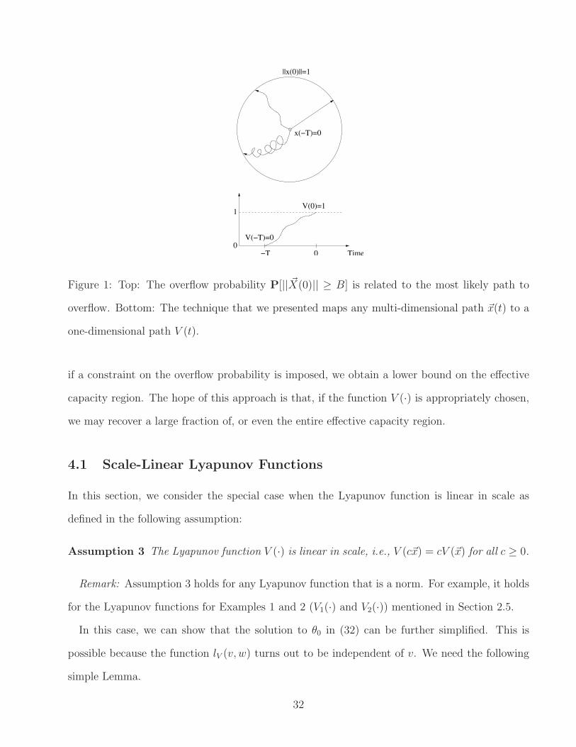
Figure 1: Top: The overflow probability P[|| ~X(0)|| ≥ B] is related to the most likely path to

overflow. Bottom: The technique that we presented maps any multi-dimensional path ~x(t) to a

one-dimensional path V (t).

if a constraint on the overflow probability is imposed, we obtain a lower bound on the effective

capacity region. The hope of this approach is that, if the function V (·) is appropriately chosen,

we may recover a large fraction of, or even the entire effective capacity region.

4.1 Scale-Linear Lyapunov Functions

In this section, we consider the special case when the Lyapunov function is linear in scale as

defined in the following assumption:

Assumption 3 The Lyapunov function V (·) is linear in scale, i.e., V (c~x) = cV (~x) for all c ≥ 0.

Remark: Assumption 3 holds for any Lyapunov function that is a norm. For example, it holds

for the Lyapunov functions for Examples 1 and 2 (V1(·) and V2(·)) mentioned in Section 2.5.

In this case, we can show that the solution to θ0 in (32) can be further simplified. This is

possible because the function lV (v, w) turns out to be independent of v. We need the following

simple Lemma.

32

Lemma 6 If (s, a,x)T is an FSP, then for any given t ∈ [−T, 0] and for any c ≥ 0, there exists

another FSP (s, a,x)cT such that

d

dt~s(t)

∣

∣

∣

∣

ct

=d

dt~s(t)

∣

∣

∣

∣

t

(36)

d

dt~a(t)

∣

∣

∣

∣

ct

=d

dt~a(t)

∣

∣

∣

∣

t

(37)

~x(ct) = c~x(t),d

dt~x(t)

∣

∣

∣

∣

ct

=d

dt~x(t)

∣

∣

∣

∣

t

(38)

Proof: Let 1B

SB(B(T + t)), 1B

AB(B(T + t)), 1B

XB(B(T + t)) be the sequence of processes that

converge to the FSP(s, a,x)T . Consider the new sequence ( 1B

SBc(B(cT + t)), 1B

ABc(B(cT +

t)), 1B

XBc(B(cT + t))) for t ∈ [−cT, 0]. In other words, we are choosing a sub-sequence from the

original sequence, and shift for a different amount of time. This new sequence can be rewritten

as c 1Bc

SBc(Bc(T + tc)), c 1

BcABc(Bc(T + t

c)), c 1

BcXBc(Bc(T + t

c)). Taking the limit as B → ∞, we

get the FSP(s, a,x)cT = (c~s( tc), c~a( t

c), c~x( t

c)). It is easy to verify that this satisfies the conditions

in (36),(37) and (38). Q.E.D.

Next we prove that under Assumption 3, lV (v, w) is independent of v.

Proposition 7 When Assumption 3 holds, the function lV (v, w) is independent of v, i.e.,

lV (v, w) = lV (cv, w)

for all c > 0.

33

Proof: Consider a fixed c > 0. According to definition (30),

lV (cv, w) = infs,a,x

H(~φ||~p) + L(~f)

subject to (s, a,x) is an FSP

such that for some t

d

dt~s(t) = ~φ

d

dt~a(t) = ~f

V (~x(t)) = cv

d

dtV (~x(t)) = w.

For any FSP(s, a,x)T and t ∈ [−T, 0] such that ddt

~s(t)∣

∣

t= ~φ, d

dt~a(t)

∣

∣

t= ~f , V (~x(t)) = v,

ddt

V (~x(t))∣

∣

t= w, according to Lemma 6, there must exist another FSP(s, a,x)cT such that

ddt~s(t)

∣

∣

ct= ~φ, d

dt~a(t)

∣

∣

ct= ~f , ~x(ct) = c~x(t), and d

dt~x(t)

∣

∣

ct= d

dt~x(t)

∣

∣

t. Using Assumption 3, we then

have

V (~x(ct)) = cv.

Further,

d

dtV (~x(t))

∣

∣

∣

∣

ct

= limτ→0

V (~x(ct + τ)) − V (~x(ct))

τ

= limτ→0

V(

~x(ct) +d~x(t)

dt

∣

∣

∣

ctτ)

− V (~x(ct))

τ

+V (~x(ct + τ)) − V

(

~x(ct) +d~x(t)

dt

∣

∣

∣

ctτ)

τ

.

34

According to Assumption 3, the first term is equal to

limτ→0

V(

~x(ct) +d~x(t)

dt

∣

∣

∣

ctτ)

− V (~x(ct))

τ

= limτ→0

V(

~x(t) + d~x(t)dt

∣

∣

∣

t

τc

)

− V (~x(t))

τ/c

=d

dtV (~x(t))

∣

∣

∣

∣

t

.

According to Assumption 1, the second term satisfies,

limτ→0

∣

∣

∣V(

~x(ct) + τ)

− V(

~x(ct) +d~x(t)

dt

∣

∣

∣

ctτ)∣

∣

∣

τ

≤ limτ→0

L0

∥

∥

∥~x(ct + τ) − ~x(ct) −

d~x(t)

dt

∣

∣

∣

ctτ∥

∥

∥

τ

= 0.

Hence, we have,

d

dtV (~x(t))

∣

∣

∣

∣

ct

=d

dtV (~x(t))

∣

∣

∣

∣

t

= w.

This implies that the FSP(s, a,x)cT satisfies the constraint in the definition of lV (cv, w). Hence,

lV (cv, w) ≤ lV (v, w)

A similar argument proves the opposite direction that lV (cv, w) ≥ lV (v, w). Since c > 0 is

arbitrary, the result then follows. Q.E.D.

35

When the function lV (v, w) is independent of v, the trajectory V (·) that attains the infimum

in (32) is in fact very easy to solve [18, p520], and the infimum is equal to infw>0lV (1,w)

w, i.e.,

θ0 = infw>0,s,a,x

1

w

[

H(~φ||~p) + L(~f)]

(39)

subject to (s, a,x) is an FSP

such that for some t

d

dt~s(t) = ~φ

d

dt~a(t) = ~f

V (~x(t)) = 1

dV (~x(t))

dt= w.

The value of θ0 has an intuitive interpretation. If we interpret w as the rate of increase of

the value of the Lyapunov function, then the objective function in (39) can be viewed as the

minimum per-unit cost to increase the Lyapunov function, where the minimization is taken over

all backlog levels ~x(t), channel states ~s(t), and arrivals ~a(t). In order to overflow, we must lift

the value of V (~x(t)) from zero to one. Hence, θ0 becomes a lower bound on the minimum cost

to overflow. According to Proposition 5, θ0 then corresponds to a lower bound on the decay rate

of the overflow probability.

5 A Condition For The Minimum-Cost-To-Overflow To

Be Exact

In the previous section, we have shown that θ0 is a lower bound on the decay rate of the queue

overflow probability (see Proposition 5). In this section, we provide a condition when the value

of θ0 becomes the exact decay-rate of the overflow probability.

Note that many scheduling policies are designed to minimize the drift of the respective Lya-

punov function, as stated in the following assumption. For any ~f, ~φ, let δki = fk

i −∑S

j=1 φj

L∑

l=1

Rileklj.

36

Define

V (τ, ~e|~x, ~φ, ~f) , V ([~x + ~δτ ]+). (40)

Then ∂∂τ

V (τ, ~e|~x, ~φ, ~f) can be viewed as the drift of the Lyapunov function from ~x(t) = ~x if

the service-rate vector is chosen as ~e, conditioned on the channel state being ~φ and ddt~a(t) = ~f .

Recall that throughout this paper, we use right-derivatives unless otherwise stated.

Assumption 4 For any FSP(s, a,x), the following holds for all t:

d

dtV (~x(t)) = min

eklj∈Conv(Ej)

∂

∂τV (τ, ~e|~x(t), ~φ(t), ~f(t)). (41)

where ~φ(t) = ddt

~s(t), ~f(t) = ddt~a(t).

This assumption states that at any point of the FSP(s, a,x), the scheduling algorithm mini-

mizes the drift of the Lyapunov function over all possible scheduling decisions.

Readers may refer to the example in Section 6 where it is shown that under a simplified version

of the cellular model of Section 2.5.1, the QLB policy minimizes the drift of the Lyapunov function

V (~x) = maxl xl.

In addition, we assume the following for the Lyapunov function.

Assumption 5 V (~x) is increasing in each component xi.

Assumption 6 V (~x1 + ~x2) ≤ V (~x1) + V (~x2) for any two vectors ~x1 ≥ 0 and ~x2 ≥ 0,

Note that Assumptions 3 and 6 combined implies that the Lyapunov function V (~x) almost

behaves as a norm except that it may not be defined for negative values of the variable ~x. We

are ready for the following proposition.

Proposition 8 Under Assumptions 1, 2, 3, 4, 5 and 6, the value of θ0 is the exact decay-rate

of the probability of overflow according to the Lyapunov function metric, i.e.,

limB→∞

1

Blog P[V (~xB(0)) ≥ 1] = −θ0. (42)

37

Further, the policy is optimal in minimizing this decay-rate. In other words, for any policy π we

must have

lim infB→∞

1

Blog Pπ[V (~xB(0)) ≥ 1] ≥ −θ0, (43)

where Pπ denote the stationary distribution under the policy π.

Remark: We will soon show that θ0 is the same as θ0 which is defined in Equation (44).

The proof of Proposition 8 contains two parts. First, we show that the decay rate of the

probability of overflow, in terms of the Lyapunov metric, is bounded from above for all scheduling

policies. Then we show that under the assumptions on the Lyapunov function, this bound

matches with the lower bound θ0.

Consider the following optimization problem:

w(~φ, ~f) = min~x

V (~x)

subject to xki = [fk

i −

S∑

j=1

φj

L∑

l=1

Rileklj]

+

[eklj] ∈ Conv(Ej) for all j.

The function w(~φ, ~f) can be viewed as the minimum rate of increase of the Lyapunov function

if the channel state is ~φ and the arrivals are ~f . Let

θ0 = inf{~φ,~f :w(~φ,~f)>0}

1

w(~φ, ~f)

[

H(~φ||~p) + L(~f)]

. (44)

We first show the following.

Proposition 9 For any policy π we must have

lim infB→∞

1

Blog Pπ[V (~xB(0)) ≥ 1] ≥ −θ0, (45)

where Pπ denotes the stationary distribution under the policy π.

Proof: By the definition of θ0, for any δ ∈ (0, 1) there exists ~φ0 and ~f0 such that

1

w(~φ0, ~f0)

[

H(~φ0||~p) + L(~f0)]

≤ θ0 + δ.

38

Further, it is easy to show that the function w(·, ·) is continuous with respect to ~φ and ~f . Hence,

there exists ǫ such that for any |~φ − ~φ0| ≤ ǫ and |~f − ~f0| ≤ ǫ, the following holds

w(~φ, ~f) ≥ w(~φ0, ~f0)(1 − δ). (46)

Let γ > 0 be a small number and let T = 1+γ

w(~φ0, ~f0)(1−δ). Define a channel-state process ~s0(·) and

an arrival process ~a0(·) on the interval [−T, 0] as follows:

~s0(t) = (t + T )~φ0 and ~a0(t) = (t + T )~f0.

Let BT (~s0(·)) denote an ǫ-ball around ~s0(·), i.e., it contains all ~s(·) such that ~s(−T ) = 0 and

||~s(t) − ~s0(t)||T∞ < ǫ.

Similarly, define an ǫ-ball BT (~a0(·)) around ~a0(·). We will now show that V (~xB(0)) ≥ 1 if

~sB(·) ∈ BT (~s0(·)) and ~aB(·) ∈ BT (~a0(·)).

From the mapping in (14), we have,

xk,Bi (0) − xk,B

i (−T +1

B) = ak,B

i (−1

B) − (47)

S∑

j=1

L∑

l=1

RilAklj

where we have used Aklj to denote

Ekl (j, B~xB(−

1

B))

[

sBj (−

1

B) − sB

j (−2

B)

]

+ . . . +

Ekl (j, B~xB(−T +

1

B))

[

sBj (−T +

1

B) − sB

j (−T )

]

.

We make the following observations to simplify (47).

xk,Bi (−T +

1

B) − xk,B

i (−T ) = O(1

B)

ak,Bi (−

1

B) − ak,B

i (0) = O(1

B)

sBj (−

1

B) − sB

j (0) = O(1

B).

39

Further, we can write Aklj =

[

sBj (− 1

B) − sB

j (−T )]

eklj where ek

lj ∈ Conv(Ej). This follows because

Ekl (j, B~xB(·)) is in the set Ej and the terms

sBj (− 1

B)−sB

j (− 2B

)

sBj (− 1

B)−sB

j (−T ), . . . ,

sBj (−T+ 1

B)−sB

j (−T )

sBj (− 1

B)−sB

j (−T )can be thought

of as weights that sum to 1. Since ~sB(−T ) = 0, we have Aklj = sB

j (− 1B

)eklj. (47) simplifies to

xk,Bi (0) − xk,B

i (−T ) = ak,Bi (0) −

S∑

j=1

L∑

l=1

RilsBj (0)ek

lj

+O(1

B).

Since xk,Bi (−T ) ≥ 0 and xk,B

i (0) ≥ 0, we can show that

xk,Bi (0) ≥

[

ak,Bi (0) −

S∑

j=1

L∑

l=1

RilsBj (0)ek

lj

]+

+ O(1

B),

Rewriting the equation using ~φ ,~sB(0)

Tand ~f ,

~aB(0)T

, we have

xk,Bi (0) + O(

1

B) ≥ T [fk

i −S∑

j=1

φj

L∑

l=1

Rileklj]

+

where eklj ∈ Conv(Ej).

Using Assumption 5 and Assumption 6 on this inequality, we obtain

V (~xB(0)) + V (O(1

B)) ≥ V (T~x)

where xki = [fk

i −S∑

j=1

φj

L∑

l=1

Rileklj]

+

This provides a bound on V (~xB(0)). However, this bound depends on the particular value of

eklj. To avoid this difficulty, we loosen the bound by allowing ek

lj to be any element of Conv(Ej).

Therefore,

V (~xB(0)) + V (O(1

B))

≥ T min V (~x)

subject to xki = [fk

i −S∑

j=1

φj

L∑

l=1

Rileklj]

+

[eklj] ∈ Conv(Ej) for all j.

40

This implies that

V (~xB(0)) + V (O(1

B)) ≥ Tw(~φ, ~f) ≥ 1 + γ,

where in the last step we have used the definition of T and the fact that (46) holds.

Therefore, there exists Bγ such that for all B > Bγ, if ~sB(·) ∈ BT (~s0(·)) and ~aB(·) ∈ BT (~a0(·))

then

V (~xB(0)) ≥ 1,

Now, using the LDP for ~sB(·) and ~aB(·), we complete the proof as follows,

lim infB→∞

1

Blog Pπ[V (~xB(0)) ≥ 1]

≥ lim infB→∞

1

B

{

log P[~sB(·) ∈ BT (~s0(·))]

+ log P[~aB(·) ∈ BT (~a0(·))]}

= − inf~s(·)∈BT (~s0(·))

∫ 0

−T

H(d

dt~s(t)||~p)dt

− inf~a(·)∈BT (~a0(·))

∫ 0

−T

L(d

dt~a(t))dt

≥ −

∫ 0

−T

H(d

dt~s0(t)||~p)dt −

∫ 0

−T

L(d

dt~a0(t))dt

= −T [H(~φ0||~p) + L(~f0)]

= −1 + γ

w(~φ0, ~f0)(1 − δ)

[

H(~φ0||~p) + L(~f0)]

≥ −1 + γ

1 − δ(θ0 + δ).

Since δ and γ can be arbitrarily small, we conclude that

lim infB→∞

1

Blog Pπ[V (~xB(0)) ≥ 1] ≥ −θ0. (48)

Q.E.D.

We are now ready to prove Proposition 8.

Proof of Proposition 8 : By Propostion 5,

lim supB→∞

1

Blog P[V (~xB(0)) ≥ 1] ≤ −θ0,

41

where θ0 is given by (39). By Proposition 9, we have

lim infB→∞

1

Blog Pπ[V (~xB(0)) ≥ 1] ≥ −θ0, (49)

for any policy π. Hence, to show Proposition 8, it only remains to show that θ0 ≥ θ0. Consider

any FSP(s, a,x) that satisfies the constraint in the definition of θ0 (see Equation (39)). Define

~φ , ddt

~s(t), ~f , ddt~a(t) and w ,

dV (~x(t))dt

. By Assumption 4, we must have

w ≤∂V (τ, ~e|~x(t), ~φ, ~f)

∂τ(50)

for any feasbile ~e.

Define ~δ = [δki , i = 1, ..., N, k = 1, ..., K], where δk

i = fki −

∑Sj=1 φj

L∑

l=1

Rileklj. We have

V (τ, ~e|~x(t), ~φ, ~f) − V (0, ~e|~x(t), ~φ, ~f)

= V ([~x(t) + ~δτ ]+) − V (~x(t))

Further, using Assumptions 3, 5 and 6, we have

V ([~x(t) + ~δτ ]+) − V (~x(t)) ≤ V (~x(t) + [~δ]+τ) − V (~x(t))

≤ V ([~δ]+τ) = τV ([~δ]+).

Hence, for any feasible ~e, by (50), we must have

w ≤ V ([~δ]+).

Minimizing the right-hand-side as in the definition of w(~φ, ~f), we have

w ≤ w(~φ, ~f).

from which we can conclude that {w > 0} ⊆ {w(~φ, ~f) > 0}. This leads to the following inequality

inf{w>0,s,a,x}

1

w

[

H(~φ||~p) + L(~f)]

≥ inf{~φ,~f :w(~φ,~f)>0}

1

w(~φ, ~f)

[

H(~φ||~p) + L(~f)]

.

42

Hence, by the definitions of θ0 (39) and θ0 (44), we have

θ0 ≥ θ0.

The result of the proposition then follows. Q.E.D.

Recall the examples discussed in Section 2.5. The Lyapunov functions V1(~x) =

√

L∑

l=1

x2l and

V2(~x) =√

∑Ni=1

∑Kk=1(x

ki )

2 mentioned in Section 3.2 can be shown to satisfy Assumptions 1, 2,

3, 4, 5 and 6. Hence, as a result of Proposition 8, we conclude that the max-weight policy is

optimal in minimizing the decay rate of P[V1(~xB(0)) ≥ 1] and that the back-pressure algorithm

is optimal in minimizing the decay rate of P[V2(~xB(0)) ≥ 1]. In the following section, we provide

another example (see Proposition 10).

6 Example

Now, we use an example to illustrate the application of the results from the previous sections.

Consider the model of a base-station serving N users described in Section 2.5.1(See Fig. 2). We

recall here the assumptions made on the arrival process and the channel model from Section 2,

and list some additional simplifying assumptions needed for our current purpose. Al(t) denotes

the number of packets generated by user l. We assume that Al(t) is i.i.d. across time and across

users. Let λl = E[Al(t)]. Only one user can be scheduled for transmission at any time. We

assume an ON-OFF channel between the base-station and the users. C(t) denotes the channel

state at time slot t and S denotes the set of all possible channel states. The probability that the

channel state C(t) at time t is j is pj. For any subset A ⊂ {1, 2, ...N}, S(A) denotes the set of

states j such that some user l ∈ A is ON. Let F denote the bandwidth of the system. Hence,

if a user’s channel is ON and it is scheduled for transmission, its service rate is F . (Remark:

The model is similar to the one in [11] although we do not assume identical arrival rates and

43

Figure 2: The scheduling problem in cellular networks under fading channel.

i.i.d. channel state distribution for the users.) The throughput-optimal Tassiulas-Ephremides

algorithm [1] in this case is the QLB (Queue-Length Based) algorithm as follows.

QLB-scheduling policy: At each time-slot t, the base-station schedules the ON user with the

largest backlog. If there are multiple ON-users that all have the largest backlog, the basestation

can schedule any one of these users.

We assume that the system is stable, which requires that there exists elj ≥ 0, l = 1, . . . , N ; j =

1, . . . , S such that∑N

l=1 elj = F for all j, and for some ǫ > 0,

λl(1 + ǫ) <∑

j∈S(l)

pjeljF for all users l = 1, . . . , N (51)

The interpretation of elj is the long-term fraction of system bandwidth given to user l in channel

state j.

In this section, we would like to charaterize the decay-rate of the tail probability of any user’s

backlog exceeding a given threshold B, i.e., the decay-rate of the probabilty

P[ maxl=1,...,N

Xl ≥ B] (52)

when B → ∞.

Define ~sB(t),~aB(t), ~xB(t) as in (1), (4) and (12), and define the fluid sample path (FSP)

accordingly. For any FSP(s, a,x), let I1(~x(t)) = {i|xi(t) = maxk xk(t)} be the set of users with

the (identically) largest queue at time t. Further, let I2(~x(t), ~x′(t)) = {i ∈ I1(~x(t))| ddt

xi(t) =

maxk∈I1(~x(t))

ddt

xk(t)}. That is, I2(~x(t), ~x′(t)) is the set of users that, among those users with the

44

largest queue at time t, also have the largest queue growth rate. In other words, these set of

users will have the largest queue immediately after time t. Then, immediately after time t, as long

as one user in I2(~x(t), ~x′(t)) is ON, according to the QLB-policy this group of users collectively

must receive the full service rate F . Therefore, we must have

∑

i∈I2(~x(t),~x′(t))

d

dtxi(t) =

∑

i∈I2(~x(t),~x′(t))

d

dtai(t) (53)

−F∑

j∈S(I2(~x(t),~x′(t)))

d

dtsj(t).

(Remark: Note that this is an example of Equation (15).)

Let V (~x) = maxl=1,...,N xl. Note that we have chosen the Lyapunov function to be the same as

the norm for the overflow metric (52). We now show the following properties of V (~x).

Proposition 10 The function V (~x) satisfies Assumptions 1, 2, 3, 4, 5 and 6.

Proof: Most of the conditions in the assumptions are easy to verify. Hence, we only provide

proofs of Assumption 1 part (f), Assumption 2 and Assumption 4.

We first show Assumption 2 part (a). Consider an FSP(s, a,x). Let ~φ(t) = ddt

~s(t) and let

~f(t) = ddt~a(t). According to the definition of I2(~x(t), ~x′(t)), the Lyapunov drift for the QLB

policy is given by

d

dtV (~x(t))

=1

|I2(~x(t), ~x′(t))|

∑

l∈I2(~x(t),~x′(t))

d

dtxl(t) (54)

=1

|I2(~x(t), ~x′(t))|

∑

l∈I2(~x(t),~x′(t))

fl(t) (55)

−F∑

j∈S(I2(~x(t),~x′(t)))

φj(t)

.

45

Let ǫ ≤ ǫminl=1,...,N λl

2(N+FS). Assume || d

dt~s(t) − ~p|| < ǫ and || d

dt~a(t) − ~λ|| < ǫ,

d

dtV (~x(t)) ≤

1

|I2(~x(t), ~x′(t))|

∑

l∈I2(~x(t),~x′(t))

λl (56)

−F∑

j∈S(I2(~x(t),~x′(t)))

pj

+ ǫ(N + FS).

By the stability condition (51), we have

∑

l∈I2(~x(t),~x′(t))

λl(1 + ǫ)

≤∑

l∈I2(~x(t),~x′(t))

∑

j∈S(l)

pjeljF

≤∑

j∈S(I2(~x(t),~x′(t)))

pjF.

Therefore, Equation (56) becomes

d

dtV (~x(t)) ≤

−ǫ

|I2(~x(t), ~x′(t))|

∑

l∈I2(~x(t),~x′(t))

λl

+ǫ(N + FS)

≤−ǫ minl=1,...,N λl

2.

This shows Assumption 2 part (a). Note that Assumption 1 part (f) can be shown with a similar

proof.

Now we show Assumption 2 part (b): By (55), and using the fact that the arrival process is

bounded by M , we have

d

dtV (~x(t)) ≤

1

|I2(~x(t), ~x′(t))|

∑

l∈I2(~x(t),~x′(t))

M

= M.

To show Assumption 4, we will first bound the Lyapunov drift for any scheduling policy and

show that the bound is in fact the drift for the QLB policy (55).

For any ~e, define δl = fl −∑S

j=1 φjelj. By definition in Equation (40),

V (τ, ~e|~x, ~φ, ~f) = V ([~x + ~δτ ]+)

= maxl=1,...,N

[xl + δlτ ]+,

46

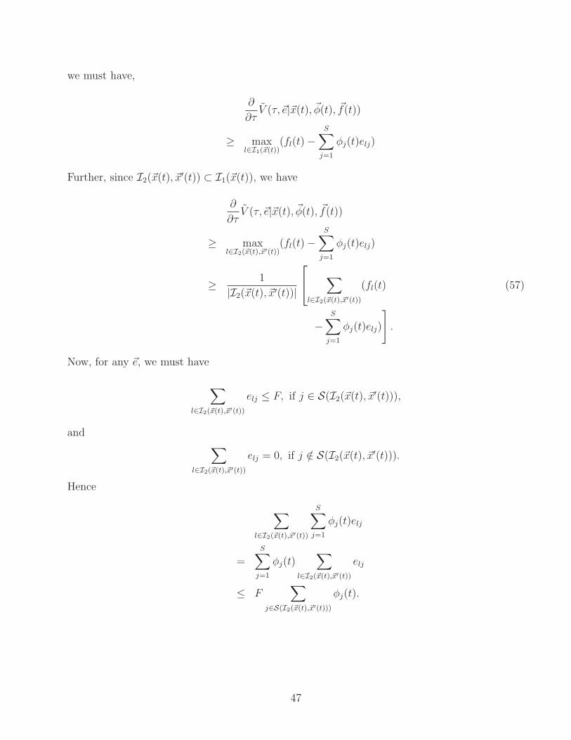
we must have,

∂

∂τV (τ, ~e|~x(t), ~φ(t), ~f(t))

≥ maxl∈I1(~x(t))

(fl(t) −S∑

j=1

φj(t)elj)

Further, since I2(~x(t), ~x′(t)) ⊂ I1(~x(t)), we have

∂

∂τV (τ, ~e|~x(t), ~φ(t), ~f(t))

≥ maxl∈I2(~x(t),~x′(t))

(fl(t) −S∑

j=1

φj(t)elj)

≥1

|I2(~x(t), ~x′(t))|

∑

l∈I2(~x(t),~x′(t))

(fl(t) (57)

−S∑

j=1

φj(t)elj)

]

.

Now, for any ~e, we must have

∑

l∈I2(~x(t),~x′(t))

elj ≤ F, if j ∈ S(I2(~x(t), ~x′(t))),

and∑

l∈I2(~x(t),~x′(t))

elj = 0, if j /∈ S(I2(~x(t), ~x′(t))).

Hence

∑

l∈I2(~x(t),~x′(t))

S∑

j=1

φj(t)elj

=S∑

j=1

φj(t)∑

l∈I2(~x(t),~x′(t))

elj

≤ F∑

j∈S(I2(~x(t),~x′(t)))

φj(t).

47

Therefore, inequality (57) reduces to

∂

∂τV (τ, ~e|~x(t), ~φ(t), ~f(t))

≥1

|I2(~x(t), ~x′(t))|

∑

l∈I2(~x(t),~x′(t))

fl(t)

−F∑

j∈S(I2(~x(t),~x′(t)))

φj(t)

where the right-hand-side is the drift of the QLB scheduler (55). The inequality (41) then follows.

The other assumptions are easily verified. Q.E.D.

By Proposition 8 and Proposition 10, we then have

limB→∞

1

Blog P[V (~xB(0)) ≥ 1] = −θ0.

where θ0 is given by

θ0 = inf{~φ,~f :w(~φ,~f)>0}

1

w(~φ, ~f)

[

H(~φ||~p) + L(~f)]

, (58)

where

w(~φ, ~f) = min[elj ]

maxl=1,...,N

xl

subject to xl = [fl −S∑

j=1

φjelj]+

[elj] ∈ Conv(Ej) for all j.

Unfortunately, (58) is not a convex program and thus not easy to solve. To derive a simpler

charaterization of θ0, we first introduce a decomposition. For any subset M ⊂ {1, 2, ..., N},

define

θ0(M) = infw>0,~φ, ~f

1

w

[

H(~φ||~p) + L(~f)]

(59)

subject to w =1

|M|

∑

l∈M

fl − F∑

j∈S(M)

φj

We then have the following results.

48

Lemma 11

θ0 = minM⊂{1,2,...,N}

θ0(M)

Proof: Fix a set M. For any ~φ, ~f , and w > 0 that satsify the constraints in (59), we automatically

have

1

|M|

∑

l∈M

fl − F∑

j∈S(M)

φj

= w.

Now, for any feasible ~e, we must have

maxl=1,...,N

[fl −S∑

j=1

φjelj]+

≥1

|M|

[

∑

l∈M

[fl −

S∑

j=1

φjelj]+

]

≥1

|M|

∑

l∈M

fl − F∑

j∈S(M)

φj

= w.

Hence, w(~φ, ~f) ≥ w, and

θ0 ≤1

w

[

H(~φ||~p) + L(~f)]

.

Since this is true for all ~φ, ~f and w > 0, we then have θ0 ≤ θ0(M). To show the other direction,

it is sufficient to show that for every ~φ and ~f , there is some M for which w = w(~φ, ~f) satisfies

the constraint (59).

Let w = w(~φ, ~f). By the definition of w(·, ·), there must exist ~e ∈ Conv(Ej) such that

maxl=1,...,N

[fl −S∑

j=1

φjelj]+ = w.

Let M be the set of l such that fl −∑S

j=1 φjelj = w. Note that we must have∑

j∈S(M) elj = F

for any state j ∈ S(M) because otherwise we should be able to further reduce maxl=1,...,N [fl −

∑Sj=1 φjelj]

+. Hence, we have

∑

l∈M

fl − F∑

j∈S(M)

φj = w|M|

49

This equation implies that ~φ, ~f and w satisfies the constraint in (59). Hence, we must have

θ0 ≥ θ0(M). The result of the lemma then follows. Q.E.D.

Next, consider the case when the arrivals are at a constant rate λl. In other words, Ll(fl) = +∞

except when fl = λl. In this case, we can use Lemma 11 to obtain the following characterization

of θ0. For any subset C of the possible channel states, let p(C) =∑

j∈C pj.

Proposition 12 When the arrivals are at a constant rate λl,

θ0 = minM⊂{1,...,N}

inf0≤u≤

P

i∈M

λiF

|M|DM(u||p)

(∑

i∈M λi) − uF

where

DM(u||p) = u logu

p(S(M))

+(1 − u) log(1 − u)

(1 − p(S(M))).

Proof: According to Lemma 11, it suffices to show that

θ0(M) = inf0≤u≤

P

i∈M

λiF

|M|

(∑

i∈M λi) − uFDM(u||p).

To see this, note that for any fixed w, θ0(M) defined in (59) corresponds to a convex program.

Associate a Lagrange multiplier η for the constraint of (59), and a Lagrange multiplier γ for the

constraint∑S

j=1 φj = 1. Ignoring the term L(~f) and letting fl = λl, we can then construct the

50

Lagrangian as

L(~φ, ~f, w, η, γ)

=S∑

j=1

φj logφj

pj

− η

[

∑

l∈M

λl

−F∑

j∈S(M)

φj − w|M|

+ γ

[

S∑

j=1

φj − 1

]

=

S∑

j=1

φj logφj

pj

+ ηF∑

j∈S(M)

φj + γφj

−η

[

∑

l∈M

λl − w|M|

]

.

It is easy to verify that, in order to minimize the Lagrangian over all ~φ, we must have

φj = pj exp[−(1 + ηF + γ)] if j ∈ S(M),

φj = pj exp[−(1 + γ)] if j /∈ S(M).

The optimal η and γ are such that the constraint of (59) and∑S

j=1 φj = 1 are both satisfied.

Hence, we must have

∑

j∈S(M)

φj = exp[−(1 + ηF + γ)]∑

j∈S(M)

pj

=

∑

l∈M λl − w|M|

F

Let u =P

l∈M λl−w|M|

F. We then have,

exp[−(1 + ηF + γ)] =u

p(S(M)).

and

φj = pju

p(S(M))if j ∈ S(M).

Similarly, we must have

∑

j /∈S(M)

φj = exp[−(1 + γ)]∑

j /∈S(M)

pj

= 1 −

∑

l∈M λl − w|M|

F= 1 − u.

51

Hence,

φj = pj(1 − u)

(1 − p(S(M)))if j /∈ S(M).

We thus have, for any fixed w, the minimum value of the objective function in (59) is equal to

1

w

S∑

j=1

φj logφj

pj

=1

w

[

u logu

p(S(M))+ (1 − u) log

(1 − u)

(1 − p(S(M)))

]

=

∑

l∈M λl − uF

|M|DM(u||p),

where in the last step we have used the definition of DM(u||p) and the assignment that u =P

l∈M λl−wM

F. Now, taking a minimum over w, or equivalently over u, the result then follows.

Q.E.D.

Remark: Readers can verify that when the channel states are i.i.d and when the arrivals from

all users are at a constant rate ~λ, Proposition 12 reduces to Theorem 5 in [11].

6.1 Effective Capacity

When the arrivals are time-varying, it is no longer possible to derive a simpler characterization

of θ0 as in Proposition 12. Instead, we can concentrate on the effective capacity region. Note

that for any θ > 0, if we would like to ensure that

limB→∞

1

Blog P[max

lXl(0) ≥ B] ≤ −θ

it is equivalent to require that θ ≤ θ0. We then have the following result. Let Ml(θ) =

log E[exp(θAl(t))], and let cl(θ) = Ml(θ)θ

. The quantity cl(θ) is typically referred to as the ef-

fective bandwidth of the system.

Proposition 13 θ ≤ θ0 is equivalent to the following condition:

∑

l∈M

|M|

θMl(

θ

|M|) ≤ −

|M|

θlog[p(S(M)) exp(−

θF

M)

+1 − p(S(M))]. (60)

52

for all M ⊂ {1, 2, ..., N}.

Remark: Given θ, Proposition 13 provides a necessary and sufficient condition on the arrival

process Al(t) for it to belong to the effective capacity region.

Proof: According to Lemma 11, we only need to show that (60) is equivalent to

θ ≤ infw>0

1

w

[

H(~φ||~p) + L(~f)]

(61)

where w =P

l∈M fl−FP

j∈S(M) φj

|M|. To see this, note that

Inequality (61)

⇔ θw ≤ H(~φ||~p) + L(~f) for all ~φ, ~f and

w =

∑

l∈M fl − F∑

j∈S(M) φj

|M|

⇔ H(~φ||~p) + L(~f) ≥θ

|M|

∑

l∈M

fl − F∑

j∈S(M)

φj

for all ~φ, ~f

⇔θ

|M|

∑

l∈M

fl − L(~f) ≤θF

|M|

∑

j∈S(M)

φj + H(~φ||~p)

for all ~φ, ~f

⇔ sup~f

θ

|M|

∑

l∈M

fl − L(~f)

≤ − sup~φ

−θF

|M|

∑

j∈S(M)

φj − H(~φ||~p)

.

Now, by definition Ll(fl) = supθ[θfl−Ml(θ)]. Using properties of Legendre transforms (Lemma 4.5.8

in [21, p152]), we have

sup~f

θ

|M|

∑

l∈M

fl − L(~f) =∑

l∈M

Ml(θ

|M|).

Similarly, by definition

H(~φ||~p) = sup~θ

{

S∑

j=1

θjφj − log E[exp(S∑

j=1

θjΦj(t))]

}

53

Hence, using the properties of Legendre transforms again, we have,

sup~φ

−θF

|M|

∑

j∈S(M)

φj − H(~φ||~p)

= log E[exp(−∑

j∈S(M)

θF

MΦj(t))]

= log[p(S(M)) exp(−θF

M) + (1 − p(S(M)))].

Hence, (61) is equivalent to

∑

l∈M

|M|

θMl(

θ

|M|) ≤

−|M|

θlog[p(S(M)) exp(−

θF

M)

+(1 − p(S(M)))].

Combining these conditions over all M, the result then follows. Q.E.D.

The quantity Ml(θ)θ

is typically refered to as the effective bandwidth of the system. The quantity

on the right-hand-side of (60) can be interpreted as the effective capacity avaiable to the users

in M. Proposition 13 then carries the intuitive explanation that the total effective bandwidth

of users in M must be no greater than the effective capacity available to them. Note that both

the effective bandwidth and effective capacity can be computed independent from each other for

any given set M.

Remark: Readers can verify that, when the channel states are i.i.d. and when arrivals from

all users are constant rate λ, Proposition 13 reduces to Corollary 6 in [11].

7 Conclusions

In this paper we study the problem of characterizing the queue-overflow probability of complex

wireless scheduling algorithms. We present a new technique for addressing the complexity issue of

the calculus-of-variations problem involved in the sample-path large deviation approach. Our new

technique combines sample-path large deviations with Lyapunov stability, which may develop

54

into a powerful approach to study a large class of scheduling algorithms. We also show that

when a scheduling algorithm minimizes the drift of the Lyapunov function, it is optimal in

maximizing the asymptotic decay-rate of the probability that the Lyapunov function values

exceed a threshold. We illustrate the potential of this approach through examples.

A Proof of Proposition 4

For ease of exposition, in this Appendix we will use the following scaling that does not involve a

shift in time (readers can compare with (1),(4) and (12)). Specifically, for t ≥ 0, let

sBj (t) =

1

B

Bt∑

τ=0

1{C(τ)=j},

ak,Bi (t) =

1

B

Bt∑

τ=0

Aki (τ),

xk,Bi (t) =

1

BXk

i (Bt),

if t = 0, 1B

, 2B

, ..., and by linear interpolation otherwise. Similarly, we define the fluid sample path

(s, a,x)T as the limit of some sequence of (sB, aB,xB) over the interval [0, T ], as B → ∞.

Pick any 0 < ρ < 1. Pick another two positive constants 0 < δ < ǫ < ρ. Let P denote the

stationary probability distribution of the system. Assume that each xB corresponds to a system

that has reached the stationary regime at time 0. We are interested in the following quantity

lim supB→∞

1

Blog P[V (~xB(0)) ≥ 1].

Let ⌈t⌉ denote the smallest integer that is greater than or equal to t. For each B, consider the

following sequence of stopping times defined on a sample path xB. (Here we use the notations

from [13].)

βB1 ,

⌈inf {t ≥ 0 : V (~xB(t)) ≤ δ}B⌉

B,

55

2B

3B

4B

5B

6B

7B

8B

9B

10B

12B

13B

δ

ρ

βB2

ηB1

βB1

ηB2

ηB,↑

V (~xB(t))

1

1B

11B

t

ǫ

Figure 3: An example of the trajectory of V (~xB(t)) and the different stopping times.

and

ηBn ,

⌈inf {t ≥ βBn : V (~xB(t)) ≥ ǫ}B⌉

B, n = 1, 2, . . .

βBn ,

⌈inf {t ≥ ηBn−1 : V (~xB(t)) ≤ δ}B⌉

B, n = 2, 3, . . .

Fig. 3 provides an example of these stopping times.

Consider the Markov chain ~xB(n) obtained by sampling ~xB(t) at the stopping times ηBn , i.e,.

~xB(n) = ~xB(ηBn ), n = 1, 2, ..., +∞. Since xB is stationary, there must also exist a stationary

distribution for the Markov chain ~xB(n). Denote this stationary distribution (of the Markov

chain ~xB(n)) by PB. Further, let ΘB denote the state space of the Markov chain ~xB(n). We can

then express the stationary distribution of ~xB(0) as (see [22, Lemma 10.1]):

P[V (~xB(0)) ≥ 1] (62)

=

∫

ΘB PB(d~x)E~x(∫ ηB

1

01{V (~xB(t))≥1}dt)

∫

ΘB PB(d~x)E~x(ηB1 )

where E~x(·) denotes the expectation conditioned on the event that ~xB(0) = ~x.

A.1 Bounding the Denominator of (62)

Consider first the denominator in (62). From (5) and the boundedness of both the arrival-

rate Aki (t) and the service-rate Ek

l (j, ~X(t)), there exists an upper bound M1 such that || ~X(t +

56

1) − ~X(t)|| ≤ M1 for all t. From Assumption 1, we have that V (~xB(ηB1 )) − V (~xB(βB

1 )) ≤

L||~xB(ηB1 ) − ~xB(βB

1 )||. Denote M0 , LM1. Hence, we must have,

V (~xB(ηB1 )) − V (~xB(βB

1 )) ≤ L||~xB(ηB1 ) − ~xB(βB

1 )||

≤ (ηB1 − βB

1 )M0.

Further, since ηB1 is the first time V (~xB(t)) exceeds ǫ, we must have

V (~xB(ηB1 )) ≥ ǫ −

M0

B.

Similarly, we have V (~xB(βB1 )) ≤ δ + M0

B. Therefore,

E~x(ηB1 ) ≥ E(ηB

1 − βB1 )

≥1

M0

(

ǫ − δ −2M0

B

)

.

Thus, there exists B1 > 0 such that for all B ≥ B1, the denominitor of (62) can be bounded

from below by

E~x(ηB1 ) ≥

ǫ − δ

2M0

. (63)

A.2 Bounding the Numerator of (62)

We next estimate the asymptotics of the numerator of (62). Recall that, by definition, each ηBn

is at most one 1B

time-unit after V (~xB(t)) just exceeds ǫ. Since ǫ < ρ, using the boundedness of

the arrival rates and the service-rates, we can conclude that there exists B2 > 0 (which depends

on ρ − ǫ), such that V (~xB(ηBn )) ≤ ρ for all B ≥ B2.

We next define the following additional stopping time (see Fig. 3 for an example):

ηB,↑ ,⌈inf {t ≥ 0 : V (~xB(t)) ≥ 1}B⌉

B.

Then, for any ~x ∈ ΘB, we must have,

E~x

[

∫ ηB1

0

1{V (~xB(t))≥1}dt

]

≤ E~x

[

1{ηB,↑≤βB1 }(β

B1 − ηB,↑)

]

.

57

The above inequality holds because: (a) if βB1 occurs before ηB,↑, then both sides will be zero;

and (b) if βB1 occurs after ηB,↑, then the amount of time V (~xB(t)) ≥ 1 must be no greater than

βB1 − ηB,↑. Let P~x denote the probability distribution conditioned on ~xB(0) = ~x. We then have

E~x

[

∫ ηB1

0

1{V (~xB(t))≥1}dt

]

≤ E~x

[

βB1 − ηB,↑|ηB,↑ ≤ βB

1

]

P~x(ηB,↑ ≤ βB

1 )

Now, E~x

[

βB1 − ηB,↑|ηB,↑ ≤ βB

1

]

is equal to E~x

{

E~x[βB1 − ηB,↑|~xB(ηB,↑), ηB,↑ ≤ βB

1 ]|ηB,↑ ≤ βB1

}

and,

due to the Markovian property of xB, we must have E~x[βB1 − ηB,↑|~xB(ηB,↑), ηB,↑ ≤ βB

1 ] =

E~xB(ηB,↑)(βB1 ). Hence,

E~x

[

∫ ηB1

0

1{V (~xB(t))≥1}dt

]

≤ E~x

[

E~xB(ηB,↑)(βB1 )|ηB,↑ ≤ βB

1

]

P~x(ηB,↑ ≤ βB

1 ).

Let C be a number that is slightly larger than 1. Using the boundedness of the arrival rates and

the service-rates again, we can find B3 > 0 such that for all B ≥ B3, V (~xB(ηB,↑)) ≤ C. Hence,

we can bound the above quantity by

E~x

[

∫ ηB1

0

1{V (~xB(t))≥1}dt

]

≤

[

sup{~y:V (~y)≤C}

E~y(βB1 )

]

P~x(ηB,↑ ≤ βB

1 ).

Let T be a positive number (which will be chosen later). Recall that V (~x) ≤ ρ for all ~x ∈ ΘB

when B ≥ B2. Hence, for any such ~x ∈ ΘB, we have,

E~x

[

∫ ηB1

0

1{V (~xB(t))≥1}dt

]

≤

[

sup{~y:V (~y)≤C}

E~y(βB1 )

]

[

P~x(ηB,↑ ≤ T )

+P~x(βB1 ≥ T )

]

≤

[

sup{~y:V (~y)≤C}

E~y(βB1 )

][

sup{~x:V (~x)≤ρ}

P~x(ηB,↑ ≤ T )

+ sup{~x:V (~x)≤ρ}

P~x(βB1 ≥ T ))

]

. (64)

58

Substituting (63) and (64) into (62), we then have, for all B ≥ max{B1, B2, B3},

P[V (~xB(0)) ≥ 1] (65)

≤2M0

ǫ − δ

[

sup{~y:V (~y)≤C}

E~y(βB1 )×

(

sup{~x:V (~x)≤ρ}

P~x(ηB,↑ ≤ T )

+ sup{~x:V (~x)≤ρ}

P~x(βB1 ≥ T )

)]

.

We next study the asymptotics for each term in the above inequality.

A.2.1 Bound for sup{~y:V (~y)≤C} E~y(βB1 )

We will show that sup{~y:V (~y)≤C} E~y(βB1 ) is bounded from above and hence does not affect the

asymptotics of (65). Due to the continuity of the Lyapunov function and the assumption that

V (~x) = 0 only if ||~x|| = 0, there exists a γ > 0 such that ||~x|| < γ implies V (~x) < δ. Further, we

can find a K > 0 such that V (~x) < C implies ||~x|| < K.

Consider the following additional stopping time

βB1 ,

⌈inf {t ≥ 0 : ||~xB(t)|| ≤ γ}B⌉

B.

It is easy to see that sup{~y:||~y||≤K} E~y(βB1 ) is an upper bound on sup{~y:V (~y)≤C} E~y(β

B1 ).

We now proceed to show that sup{~y:||~y||≤K} E~y(βB1 ) is bounded from above. From Assumption 1,

the fluid limit of the system satisfies either (21) or (22). For both cases, it follows that there

exists a constant t0 such that for all fluid limits x with ||~x(0)|| ≤ 1, we must have ||~x(t0)|| = 0.

This not only implies that the original system is stable (see [19, Theorem 4.2]), but also leads to

the following limit:

lim||~x||→∞

1

||~x||E[

~X(t0||~x||)∣

∣

∣

~X(0) = ~x]

= 0.

(See the proof of Theorem 4.2 in [19]). Then using the techniques in the proof of Theorem 3.1

in [19], there must exist numbers ǫ > 0, κ > 0, b ≥ 0, and a bounded set B , { ~X : || ~X|| ≤ κ}

59

such that for all ~x, conditioned on ~X(0) = ~x, the following holds,

E[τB(t0)| ~X(0) = ~x] ≤t0ǫ

(||~x|| + b),

where τB(t0) , inf{t ≥ t0 : ~X(t) ∈ B} is the first time after t0 when ~X(t) returns to the set B.

Recall the transformation ~xB(t) = 1B

~X(Bt), t = 0, 1B

, 2B

, .... For all B ≥ κγ, as long as

|| ~X(Bt)|| ≤ κ, it implies that ||~x(t)|| ≤ γ and thus βB1 ≤ t. Hence, for any ~y such that ||~y|| ≤ K

and for any B ≥ κγ, the following holds

E~y(βB1 ) ≤

1

BE[τB(t0)| ~X(0) = B~y]

≤t0ǫB

(B||~y|| + b).

Let B5 = max{κγ, b

K}. Then, for all B ≥ B5, we have,

sup{~y:V (~y)≤C}

E~y(βB1 ) ≤ sup

{~y:||~y||≤K}

E~y(βB1 ) ≤ 2

Kt0ǫ

. (66)

A.2.2 Asymptotics for sup{~x:V (~x)≤ρ} P~x(ηB,↑ ≤ T )

Let

Γ≤ρ , {x : V (~x(0)) ≤ ρ and V (~x(t)) ≥ 1

for some t ∈ (0, T ]}

Then, by Proposition 2, we have

lim supB→∞

1

Blog sup

{~x:V (~x)≤ρ}

P~x(ηB,↑ ≤ T )

= lim supB→∞

1

Blog sup

{~x:V (~x)≤ρ}

P~x(xB ∈ Γ≤ρ)

≤ − infall FSP(s,a,x)T :x∈Γ≤ρ

∫ T

0

[

H

(

d

dt~s(t)||~p

)

+ L

(

d

dt~a(t)

)]

dt. (67)

60

A.2.3 Asymptotics for sup{~x:V (~x)≤ρ} P~x[βB1 ≥ T ]

Let

Υ≤ρ , {x : V (~x(0)) ≤ ρ and V (~x(t)) > δ

for all t ∈ [0, T − 1]}.

Then, by Proposition 2, we have

lim supB→∞

1

Blog sup

{~x:V (~x)≤ρ}

P~x[βB1 ≥ T ]

≤ lim supB→∞

1

Blog sup

{~x:V (~x)≤ρ}

P~x[xB ∈ Υ≤ρ]

≤ − infall FSP(s,a,x)T :x∈Υ≤ρ

∫ T−1

0

[

H

(

d

dt~s(t)||~p

)

+ L

(

d

dt~a(t)

)]

dt. (68)

For any FSP (s, a,x)T such that x ∈ Υ≤ρ, we have

δ ≤ V (~x(0)) +

∫ T−1

0

d

dtV (~x(t))dt

≤ ρ +

∫ T−1

0

d

dtV (~x(t))dt.

We now need to use Assumption 2. Since the two parts in Assumption 2 are equivalent, in the

following we will assume the latter part holds‡. Let η be defined as in Assumptions 1 and 2.

Then, according to Assumption 2, there exists ǫ′ > 0 such that for all FSPs (s, a,x)T , if at any

time t we have || ddt

~s(t) − ~p|| ≤ ǫ′ and || ddt~a(t) − ~λ|| ≤ ǫ′, then the following holds

d

dtV (~x(t)) ≤ −η/2.

Further, there exists M1 ≥ 0 such that if at any time t we have || ddt

~s(t)−~p|| ≥ ǫ′ or || ddt~a(t)−~λ|| ≥

ǫ′, then the following holds

d

dtV (~x(t)) ≤ M1.

‡If the first part of Assumption 2 holds, the following proof can be easily modified by using the Lyapunov

function U(~x) = V1−α(~x)1−α

.

61

Let M denote the set of (~φ, ~f) such that ||~φ − ~p|| ≤ ǫ′ and ||~f − ~λ|| ≤ ǫ′. We then have,

δ ≤ ρ +

∫ T−1

0

[

−η

21{( d

dt~s(t), d

dt~a(t))∈M}

+M11{( ddt

~s(t), ddt

~a(t))/∈M}

]

dt.

Hence,

(

M1 +η

2

)

∫ T−1

0

1{( ddt

~s(t), ddt

~a(t))/∈M}dt

≥ (T − 1)η

2+ δ − ρ. (69)

Let

Jmin = min~φ,~f

J(~φ, ~f)

subject to ||~φ − ~p|| ≥ ǫ′ or ||~f − ~λ|| ≥ ǫ′.

It is easy to see that Jmin is positive. Thus, for any FSP (s, a,x)T such that x ∈ Υ≤ρ, we have

∫ T

0

[

H

(

d

dt~s(t)||~p

)

+ L

(

d

dt~a(t)

)]

dt (70)

≥

∫ T−1

0

Jmin1{( ddt

~s(t), ddt

~a(t))/∈M}dt

≥(T − 1)η

2+ δ − ρ

M1 + η/2Jmin.

where the last inequality follows from (69). Substituting into (68), we then have

lim supB→∞

1

Blog sup

{~x:V (~x)≤ρ}

P~x[βB1 ≥ T ] (71)

≤ −(T − 1)η

2+ δ − ρ

M1 + η/2Jmin.

Clearly, for fixed δ and ρ, by choosing large T , we can make the right-hand-side arbitrarily small.

62

A.3 Completing the Proof of Proposition 4

We are now ready to prove the statement of Proposition 4. Pick any FSP (s, a,x)T0 such that

~x(0) = 0, V (~x(T0)) ≥ 1. Suppose the cost of this FSP is J , i.e.

∫ T0

0

[

H

(

d

dt~s(t)||~p

)

+ L

(

d

dt~a(t)

)]

dt = J .

Clearly, for any T ≥ T0, the right-hand-side of (67) must be no smaller than −J . According to

(71), for fixed δ and ρ there must exist T1 > T0 (which is independent of ρ), such that for all

T ≥ T1, the right-hand-side of (71) is smaller than −J . Fix such a T ≥ T1. Substituting (66),

(67) and (71) into (65), and taking the appropriate limits, we then have,

lim supB→∞

1

Blog P[V (~xB(0)) ≥ 1]

≤ − infall FSP(s,a,x)T :x∈Γ≤ρ

∫ T

0

H

(

d

dt~s(t)||~p

)

+L

(

d

dt~a(t)

)

dt.

Note that the above inequality holds for all ρ > 0. Let Jρ denote the infimum on the right-hand-

side. As ρ → 0, let J∗ denote the limit, i.e., J∗ = limρ→0 Jρ. We then have

lim supB→∞

1

Blog P[V (~xB(0)) ≥ 1] ≤ −J∗.

Let

J0 = infall FSP(s,a,x)T :

~x(0)=0,V (~x(T ))≥1

∫ T

0

H

(

d

dt~s(t)||~p

)

+L

(

d

dt~a(t)

)

dt.

It only remains to show that J∗ ≥ J0. To see this, take a sequence ρn → 0. There must exist a

sequence of FSPs (sn, an,xn)T such that V (~xn(0)) ≤ ρn and V (~xn(T )) ≥ 1 for each n, and

limn→∞

∫ T

0

[

H

(

d

dt~sn(t)||~p

)

+ L

(

d

dt~an(t)

)]

dt = J∗.

63

Take a further subsequence that converges uniformly over compact intervals. Without loss of

generality, we can denote this subsequence also by (sn, an,xn)T , and let (s, a,x)T be the corre-

sponding limit. Then, using the lower-semicontinuity of the cost function, we must have

∫ T

0

H

(

d

dt~s(t)||~p

)

+ L

(

d

dt~a(t)

)

dt ≤ J∗.

Using a similar argument as in the proof of Propositon 2, we can show that (s, a,x)T is also an

FSP, and it satisfies the condition that x(0) = 0 and V (x(T )) ≥ 1. Hence, it belongs to the set

of FSP in the constraint set in (72). We thus have J0 ≤ J∗. In other words, we have shown that

for all T ≥ T1,

lim supB→∞

1

Blog P[V (~xB(0)) ≥ 1]

≤ − infall FSP(s,a,x)T :

~x(0)=0 and V (~x(T ))≥1

∫ T

0

H

(

d

dt~s(t)||~p

)

+L

(

d

dt~a(t)

)

dt.

Note that the above inequality is for a fixed T ≥ T1. Note that the infimum on the right-hand-

side decreases as T increases. Hence, taking another infimum over all T > 0, we must then

have

lim supB→∞

1

Blog P[V (~xB(0)) ≥ 1]

≤ − infall FSP(s,a,x)T ,T>0:

~x(0)=0 and V (~x(T ))≥1

∫ T

0

H

(

d

dt~s(t)||~p

)

+L

(

d

dt~a(t)

)

dt.

The result of the proposition then follows with a trivial change of the origin of time.

References

[1] L. Tassiulas and A. Ephremides, “Stability Properties of Constrained Queueing Systems

and Scheduling Policies for Maximum Throughput in Multihop Radio Networks,” IEEE

64

Transactions on Automatic Control, vol. 37, no. 12, pp. 1936–1948, December 1992.

[2] F. P. Kelly, “Effective Bandwidth in Multiclass Queues,” Queueing Systems, vol. 9, pp.

5–16, 1991.

[3] A. I. Elwalid and D. Mitra, “Effective Bandwidth of General Markovian Traffic Sources

and Admission Control of High Speed Networks,” IEEE/ACM Transactions on Networking,

vol. 1, no. 3, pp. 329–343, June 1993.

[4] G. Kesidis, J. Walrand, and C.-S. Chang, “Effective Bandwidth for Multiclass Markov

Fluids and other ATM Sources,” IEEE/ACM Transactions on Networking, vol. 1, no. 4, pp.

424–428, Aug. 1993.

[5] D. D. Botvich and N. G. Duffield, “Large Deviations, the Shape of the Loss Curve, and

Economies of Scale in Large Multiplexers,” Queueing Systems, vol. 20, pp. 293–320, 1995.

[6] N. G. Duffield and N. O’Connell, “Large deviations and overflow probabilities for the general

single server queue, with application,” Math. Proc. Cambr. Phil. Soc., vol. 118, pp. 363–374,

1995.

[7] C. Courcoubetis and R. Weber, “Buffer Overflow Asymptotics for a Buffer Handling Many

Traffic Sources,” Journal of Applied Probability, vol. 33, pp. 886–903, 1996.

[8] D. Wu and R. Negi, “Effective Capacity: A Wireless Link Model for Support of Quality of

Service,” IEEE Transactions on Wireless Communications, vol. 2, no. 4, pp. 630–643, July

2003.

[9] A. Eryilmaz and R. Srikant, “Scheduling with Quality of Service Constraints over Rayleigh

Fading Channels,” in Proceedings of the IEEE Conference on Decision and Control, Decem-

ber 2004.

65

[10] S. Shakkottai, “Effective Capacity and QoS for Wireless Scheduling,” IEEE Transactions

on Automatic Control, vol. 53, no. 3, April 2008.

[11] L. Ying, R. Srikant, A. Eryilmaz, and G. E. Dullerud, “A Large Deviations Analysis of

Scheduling in Wireless Networks,” IEEE Transactions on Information Theory, vol. 52,

no. 11, November 2006.

[12] D. Bertsimas, I. C. Paschalidis, and J. N. Tsitsiklis, “Asymptotic Buffer Overflow Proba-

bilities in Multiclass Multiplexers: An Optimal Control Approach,” IEEE Transactions on

Automatic Control, vol. 43, no. 3, pp. 315–335, March 1998.

[13] A. L. Stolyar, “Large Deviations of Queues Sharing a Randomly Time-varying Server,”

Queueing Systems, vol. To appear, 2008.

[14] X. Lin, “On Characterizing the Delay Performance of Wireless Scheduling Algorithms,” in

44th Annual Allerton Conference on Communication, Control, and Computing, Monticello,

IL, September 2006.

[15] V. J. Venkataramanan and X. Lin, “On Wireless Scheduling Algorithms for Minimizing the

Queue-Overflow Probability,” submitted to IEEE/ACM Trans. on Networking, 2008.

[16] A. Dembo and O. Zeitouni, Large Deviations Techniques and Applications, 2nd ed. New

York: Springer-Verlag, 1998.

[17] A. Eryilmaz, R. Srikant, and J. Perkins, “Stable Scheduling Policies for Fading Wireless

Channels,” IEEE/ACM Transactions on Networking, vol. 13, no. 2, pp. 411–424, April

2005.

[18] A. Shwartz and A. Weiss, Large Deviations for Performance Analysis: Queues, Communi-

cations, and Computing. London: Chapman & Hall, 1995.

66

[19] J. G. Dai, “On Positive Harris Recurrence of Multiclass Queueing Networks: A Unified

Approach via Fluid Limit Models,” Annals of Applied Probability, vol. 5, no. 1, pp. 49–77,

1995.

[20] M. J. Neely, E. Modiano, and C. E. Rohrs, “Dynamic Power Allocation and Routing for

Time Varying Wireless Networks,” IEEE Journal on Selected Areas in Communications,

Special Issue on Wireless Ad-Hoc Networks, vol. 23, no. 1, pp. 89–103, January 2005.

[21] A. Dembo and O. Zeitouni, Large Deviations Techniques and Applications. Boston: Jones

and Bartlett, 1993.

[22] A. L. Stolyar, “Control of End-to-End Delay Tails in a Multiclass Networks: LWDF Disci-

pline Optimality,” Annals of Applied Probability, vol. 13, no. 3, pp. 1151–1206, 2003.

67