on the quantum equivalence principle · physics b on the quantum equivalence principle ... only the...

Nuclear Physics B415 (1994) 243-261 North-Holland

NUCLEAR PHYSICS B

On the Quantum Equivalence Principle

Hermann Hessling Deutsches Elektronerdynchrotron (DESY), Notkestrasse 85, D-22603 Hamburg, Germany

Received 25 January 1993 Accepted for publication 3 November 1993

According to Galilei “all bodies fall with the same speed”. How can the idea, upon which Einstein’s explanation of this fact is founded, be transferred into quantum field theory? A formulation of a Quantum Equivalence Principle (QEP) is suggested here. It is applicable to linear quantum field theories but cannot be applied directly to interacting quantum fields. Equilibrium states of free quantum fields in the Rindler wedge are analyzed and it is shown that only the state with the Hawking-Bisognano-Wichmann temperature is admitted by the Quan- tum Equivalence Principle.

1. Introduction

Galilei was the first to realize that gravitational and inertial mass are equivalent. He discovered that gravity acts on all bodies in such way that they fall with the same speed. Other forces have been found but none of these show this behavior of equivalence. For example electrons and positrons in an electromagnetic field move in different directions.

Einstein gave a paradoxical explanation of the equivalence principle: “locally” there is no gravity.

Consider a classical pointlike testparticle in a gravitational field. In every point of the worldline it is possible to find a coordinate system (“local inertial system”) where the equation of motion looks trivial, i.e. does not differ from the equation of motion in the absence of gravitation. To observe gravitational effects the worldline has to be considered in some neighborhood of a point and not only in a single point. The influence of gravitation on other classical objects, e.g. classical fields, can also be transformed away pointwise by choosing a local inertial system.

It is not so clear how to describe the influence of gravitation on quantum fields because on the one hand the Equivalence Principle is a consequence of the small-distance behavior of the gravitational force but on the other hand the small-distance behavior of quantum fields is singular.

0550-3213/94/$07.00 8 1994 - Elsevier Science B.V. All rights reserved

244 H. Hessling / Quantum equivalence principle

The small-distance behavior of quantum field theories is related to the problem of characterizing “physically realizable states”. In quantum field theories in Minkowski spacetime energy plays an important role in describing physically realizable states. Since in experiments only a finite amount of energy is available, only those states have to be considered as physically realizable whose energy differs by a finite amount from the energy of the vacuum state. This suggests that all physically realizable states are locally quasi-equivalent * to the vacuum state 1141.

Because of its translation invariance and invariance under Lorentz transforma- tions the vacuum state is a distinguished state from a geometrical point of view. Moreover the vacuum state is (in its GNS representation) a ground state of the generator of the time evolution along the time axis of an inertial coordinate system. In curved spacetimes there exists no global inertial system. For that reason one cannot in general define a “vacuum state” in a curved spacetime. Is it possible to characterize physically realizable states without knowledge of a reference state? The Principle of Local Definiteness (PLD) of Haag, Namhofer and Stein [13] postulates: physically realizable states are locally quasi-equivalent. The physical content of this principle is that the expectation values (A), (A)’ of a field observable A in the physically realizable states ( >, ( >’ become indistinguishable as the localization region of A is contracted to a point. There are criteria in the case of linear quantum fields in the Robertson-Walker spacetime from which the PLD follows [1,17].

A general characterization of physically realizable states in curved spacetimes has not been given till now, but the concept of the scaling limit ofstates introduced by Fredenhagen and Haag [ll] is of great importance in this context. The scaling limit allows the formulation of a Principle of Locul Stability (PLS): the scaling limit of a state in a curved spacetime does not differ from the scaling limit of the vacuum state in Minkowski spacetime [13,11]. But local stability is not sufficient to fix the quasi-equivalence class of a state. A counterexample in connection with the Robertson-Walker spacetime has already been given in ref. [13]. Another counterexample in connection with the problem of the Hawking temperature will be discussed in sect. 3.

The general concepts just mentioned are well explained in the case of Hadamard states. Hadamard states are definable in linear quantum field theories and are

l Let (A) be the expectation value of a field observable A localized in a finite spacetime region. It is possible (via the GNS construction; e.g. ref. [14D to obtain a Hilbert space 2’ and in this Hilbert space X a representation 7~ of the field observables as linear operators r(A). A state ( )’ is locally quasie-equivalent to the state (> if it is representable by a density matrix p in the Hilbert space Z: (A)‘=Trprr(A).

H. Hessling / Quantum equivalence principle 24.5

quasifree states l with a specific singularity structure: the symmetric part of the two-point function is identical with Hadamard’s fundamental solution of the wave equation [lo]

((+(P’), &(P)})=u/u+u ln u+w. (1)

The functions U, U, w are regular in P and P’. The information about the state is contained in w; u and u are state-independent. In the limit where the localization points P, P’ of the quantum field C$ coincide (“scaling limit”) only the most singular term u/u contributes. According to the Principle of Local Stability the u/a term has to be compared with the most singular part of the vacuum state of the quantum field C$ in the Minkowski spacetime. This gives the right “ie prescription”, i.e. the interpretation of the l/a singularity in the sense of distributions. It was shown by Verch [21] that Hadamard states satisfy the PLD, i.e. Hadamard states are “physically realizable”.

There is a conjecture by Haag [14] that quasifree states fulfill the PLD, if the symmetric part of their two-point functions allows an expansion

({4(P’)> 4(P)D = -1 l 279 cr(P’, P) +Aw(P’, P) (2)

in which the leading singularity is proportional to the square of the geodesic distance CT between P’ and P, i.e. has a singularity of order two, and if Aw has a singularity of order less than one. Hadamard states fulfill the assumptions of Haag’s conjecture.

The motivation of Haag, Narnhofer and Stein [13] to introduce the PLD was to understand the Hawking temperature of black holes [15] from a fundamental point of view. They consider KMS states ** with respect to the timelike Killing vector field of a black hole and showed that the only KMS state, which fulfills the PLS, is the one with the Hawking temperature. But their derivation of the Hawking temperature has some shortcomings. They used a very singular scaling procedure, not in accordance with the prescription of ref. [ll], and put one point of the two-point function of the KMS state on the intersection of the past and future horizon of a static black hole. But a realistic black hole is the final state of a collapsed star and there is no past horizon. As we will show, the PLS is not sufficent, but the QEP is needed in the case of a realistic black hole in order to arrive at the Hawking temperature as the unique equilibrium temperature of a black hole.

In sect. 2 we attempt a formulation of the QEP. While this appears appropriate

l A state is called quasifree, if its truncated n-point functions vanish for n + 2. l * KMS = Kubo, Martin, Schwinger [16,18].

246 H. Hassling / Quantum equivalence principle

for linear fields it is not directly applicable in asymptotically free theories like QCD l .

In sect. 3 the QEP is applied to equilibrium states of Klein-Gordon and Dirac fields in the Rindler wedge to demonstrate that it leads to some interesting physical insights even for linear theories. Especially it is shown that only one equilibrium state is allowed by the QEP, the one with the Hawking-Bisognano- Wichmann temperature. The result for the Dirac field disproves a statement in ref. [191.

2. Quantum Equivalence Principle

In General Relativity the gravitational field is represented by the metric tensor. It is always possible to introduce coordinates Pp = (t, x, y, z) around an arbitrary point P, in spacetime in such a way that the components of the metric tensor grV in P, coincide with the components of the Minkowski metric vclV = diag(1, - 1, - 1, - 1) and the partial derivatives vanish,

g,,(P*) =77/L”) q&Lv(p*) =o* (3) Such a coordinate system is called a local inertial system around P, . The physical meaning of eqs. (3) is that the gravitational field can be transformed away in an infinitesimal neighborhood of P, . There is no gravitation “locally”. Gravitation is an effect of second order. This explains the experimentally very well tested Equivalence Principle: “All bodies fall with the same speed” (Galilei).

We want to transfer Einstein’s idea, that the influence of gravitation is observable only beyond the first order, to other interactions. Are there interactions which vanish at small length scales, comparable to the gravitational force? Since the other fundamental classical interaction, electromagnetism, does not show this behavior we have to got to the quantum level. If there should be an interaction with this short-distance behavior this would show that there is a QEP.

We first concentrate on the problem how to define quantum field theories which are “free up to first order”. This is a nontrivial task, because the short-distance behavior of quantum fields is singular even in the linear case.

To begin with, we remark that the content of eqs. (3) can be reformulated as follows: there is a coordinate system Pp = (t, x, y, z) around P, such that for all

l One of the referees of this paper mentioned that the term “Quantum Equivalence Principle” has already been introduced in the literature. This was not known to us. The definition presented in ref. [22] is interesting but differs from our notation. It is formulated as some differential conditions on a hypersurface. But a hypersurface is a global concept and exactly this global aspect does not fit into our understanding of the QEP as a principle which describes the behavior of nature at small distances like the Equivalence Principle.

H. Hessling / Quantum equivalence principle

points P in a small neighborhood around P,

where (with respect to this coordinate system)

(XhP)I’ = P”, + A( P” - P*F)

241

(4)

(5)

is a one-parametric scaling diffeomorphism with xlP = P and ,yoP = P,. In the limit A + 0 the point P is scaled into the point P, along the path defined by the diffeomorphism A*. The first equation in (4) gives the “value” of the metric tensor in the scaling point P, by a one-parametric scaling procedure. The second equation in (4) means that the metric tensor is “constant up to first order in A”.

A one-parametric scaling procedure is also customary to analyze the short-distance behavior of quantum fields. For simplicity we consider in this section the case of a scalar quantum field 4(P). We assume that the field 4 has been renormalized relative to the state ( >.

The one-parametric diffeomorphisms xA give rise to of an action (Y* on products of the quantum field l ,

(6)

In the limit A --) 0 the localization points P,, . . . , P,, of the product c$(P,). . . c$<P,,> move under the action of (Y* along the path ,Y~ into the point P, . In addition each field c#I<P$ is scaled by a function N(A). The scaling jimction N(h) is important to define the short-distance behavior of products of the quantum field.

The state ( ) has a scaling limit [ll] in the point P, if there is a scaling function N(A), which is monotonous and nonnegative for A > 0, such that for every n-point function (t#dP,). . . d(P,J) the limit

exists and is nonzero for some n. The right hand side of (7) can be considered as the “value” of the n-point

function in the scaling point P, . It was shown by Fredenhagen and Haag [ill that the scaling limit wP ,,,,,, P, (P,) is independent of the choice of the coordinate system, i.e. the special diffeomorphism ,yh may be replaced by a general contrac- tive one which has the point P, as a fixpoint.

l The existence of the products is to be understood in the sense of distributions, i.e. (6) has to be smeared out with test functions f(“XPI,. . ., P,,) with supports contained in d X . . . X U = d”, d being a region in spacetime.


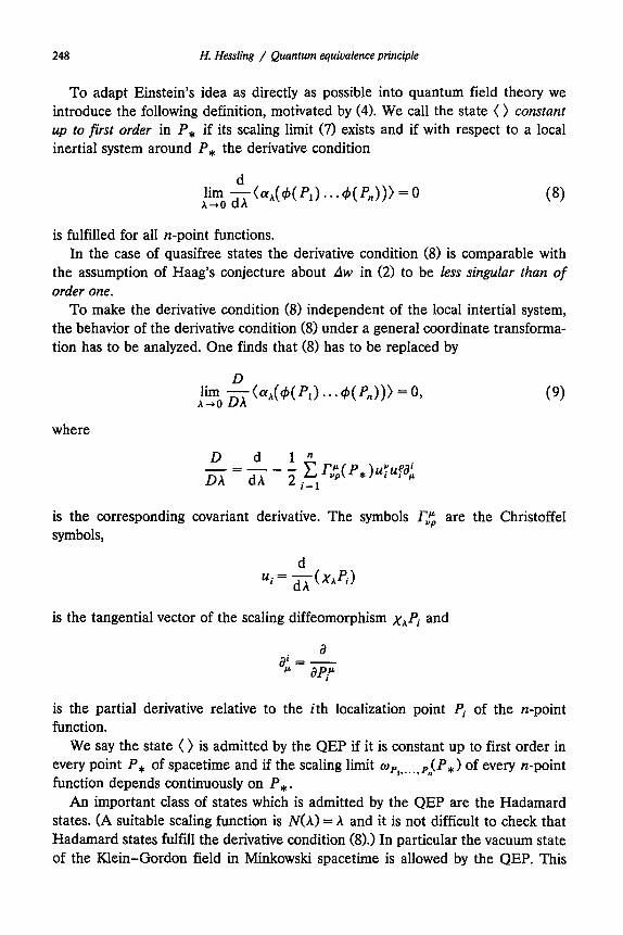
To adapt Einstein’s idea as directly as possible into quantum field theory we introduce the following definition, motivated by (4). We call the state ( > constunf up to first order in P, if its scaling limit (7) exists and if with respect to a local inertial system around P, the derivative condition

is fulfilled for all n-point functions. In the case of quasifree states the derivative condition (8) is comparable with

the assumption of Haag’s conjecture about Aw in (2) to be less singular than of order one.

To make the derivative condition (8) independent of the local intertial system, the behavior of the derivative condition (8) under a general coordinate transformation has to be analyzed. One finds that (8) has to be replaced by

where

D d 1” -=--- DA dh 2 c qxp*)GP;

i-l

is the corresponding symbols,

covariant derivative. The symbols ry”, are the Christoffel

is the tangential vector of the scaling diffeomorphism XhPi and

is the partial derivative relative to the ith localization point Pi of the n-point function.

We say the state ( > is admitted by the QEP if it is constant up to first order in every point P, of spacetime and if the scaling limit up,, . , pJP.+ > of every n-point function depends continuously on P, .

An important class of states which is admitted by the QEP are the Hadamard states. (A suitable scaling function is N(h) = A and it is not difficult to check that Hadamard states fulfill the derivative condition (81.1 In particular the vacuum state of the Klein-Gordon field in Minkowski spacetime is allowed by the QEP. This

H. Hessling / Quantum equivalence principle 249

shows that at least for linear quantum field theories the QEP can be a criterion which selects theories free up to first order (in A).

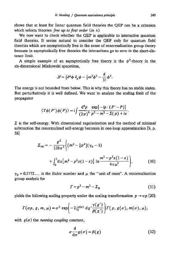
We now want to check whether the QEP is applicable to interactive quantum field theories. It seems natural to consider the QEP only for quantum field theories which are asymptotically free in the sense of renormalization group theory because in asymptotically free theories the interactions go to zero in the short-distance limit.

A simple example of an asymptotically free theory is the +3-theory in the six-dimensional Minkowski spacetime,

The energy is not bounded from below. This is why this theory has no stable states. But perturbatively it is well defined. We want to analyze the scaling limit of the propagator

d6p exp[-ip*(P’-P)] <zy(P’)4(P)) =q-

(&+ p2-m2-X(p) +iE *

S is the self-energy. With dimensional regularization and the method of minimal subtraction the renormalized self-energy becomes in one-loop approximation [9, p. 581

&= -$ i (m2 - ;P’)<rE - 1)

+j1dx[m2-p2x(1 -x)1 ln 0

yE = 0.5772. . . is the Euler number and ,u the “unit of mass”. A renormalization group analysis for

r=p2-m2-& (11)

yields the following scaling property under the scaling transformation p --) ap [20]:

r(ap, g, m, CL) =u2 exp qP9 g(4 m(a), A4

with g(a) the running coupling constant,

(12)


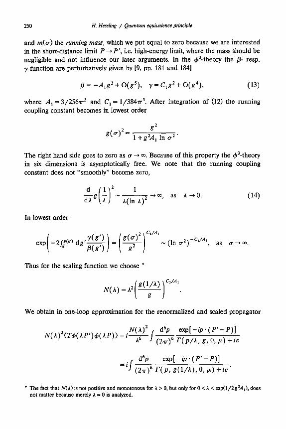
and m(a) the running muss, which we put equal to zero because we are interested in the short-distance limit P + P’, i.e. high-energy limit, where the mass should be negligible and not influence our later arguments. In the 43-theory the /3- resp. y-function are perturbatively given by [9, pp. 181 and 1841

p = -A,g3 + O(2), Y = Cl&? + O(g4), (13)

where A, = 3/256r3 and C, = 1/384rr3. After integration of (12) the running coupling constant becomes in lowest order

kw2 = g2 1 +g2A, In u2 ’

The right hand side goes to zero as u + 03. Because of this property the +3-theory in six dimensions is asymptotically free. We note that the running coupling constant does not “smoothly” become zero,

1

A(ln A)* --) m, as A+O. (14)

In lowest order

N (In u2) -c1'A1, as u-03.

Thus for the scaling function we choose *

We obtain in one-loop approximation for the renormalized and scaled propagator

NW2 d6p exp[-ip*(P’-P)] N(A)*(T~(AP’)$J(AP)> =i~/-

(2,# r( PA g, 0, CL) f is

. d% /

exp[-ip*(P’-P)] =z

(2~)~ r( P, g(l/A), 0, CL) + i& ’

l The fact that N(h) is not positive and monotonous for A > 0, but only for 0 <A < exp(l/2g2A,), does not matter because merely A = 0 is analyzed.

H. Hess&g / Quantum equivalence principle 2.51

If we differentiate with respect to A, we see by using (lo), (11) and (141, that the limit A + 0 diverges and the derivative condition (8) of the QEP is not fulfilled. This is due to the property of the running coupling constant g(l/h) that it does not smoothly become zero in the short-distance limit A + 0.

From the viewpoint of perturbation theory QCD is very similar to the 43-theory in six dimensions *. Therefore the QEP does not harmonize with QCD. This means that the derivative condition (8) has to be modified if one wants to formulate a QEP for interactive quantum field theories.

3. Equilibrium states in the Rindler wedge

In this section we calculate equilibrium states of a Klein-Gordon field 4(P) and a Dirac field e(P) in the Rindler wedge and investigate with the QEP which temperatures are physically allowed.

In quantum mechanics of finite degrees of freedom equilibrium states are characterized by

(A) = Tr( e-‘?A)

Tr e-flH ’ (15)

where H is the Hamilton operator and A an observable. They are equally well described by the KMS boundary condition

(A,N = OA,,,,). (16) A

7 = eiHrAe-iHr is the time translated observable A. In quantum field theory the right hand side of (15) does not exist. But the KMS

boundary condition (16) remains valid [12]. Therefore equilibrium states in quantum field theory are considered as KMS states:

Let r ‘-‘A, be the time evolution of a field observable A. A KMS state ( > with the temperature l//3 relative to this time evolution is characterized by the conditions that (&I,+,,> considered as a function in r + is is analytic in the strip 0 < E < p and that ( B,4,+i,) fulfills in the limit E + /3 the KMS boundary condition (16) [12,8,14].

We first consider the Klein-Gordon field and choose as the observable the field itself A = 4(P). The time evolution is defined via the one-parametric group of automorphisms

I- b-b 4,(P) = 4(A,P), (17)

l The p- and y-functions formaliy have the same perturbative expansions as (13).


where P, = A,P is the one-parametric group of diffeomorphisms defined by

P, describes a velocity transformation in the x-direction which leaves the Rindler wedge

W-={P@I Itl <xl

invariant. The coordinates (t, x, y, 2,) are the standard inertial coordinates of the Minkowski spacetime (ds* = dt2 - dx2 - dy2 - dz2). These coordinates are regular not only in the Rindler wedge W but also on the horizon I t 1 =x of the Rindler wedge.

By Fourier transforming the KMS boundary condition and by using their analytical properties KMS states are representable in terms of the commutator function. Assuming a vanishing one-point function ( c#A PI) one has for P’, P E W

=-+‘([$,.(P), ~(P’)])coth$(+r-k). (19

The crucial point is that in linear field theories the commutator function is state-independent. Thus equilibrium states of the Klein-Gordon field are com- putable via (19). For the nonequal time commutator of a massless Klein-Gordon field one finds

Lb(P), W’)l = & sign(t-t’)G(u(P, P’)), (20)

where

o(P, P’)=(t-tr)2-(X-x~)2 (21)

is the square of the geodesic distance between P, P’ and sign(t) the sign function


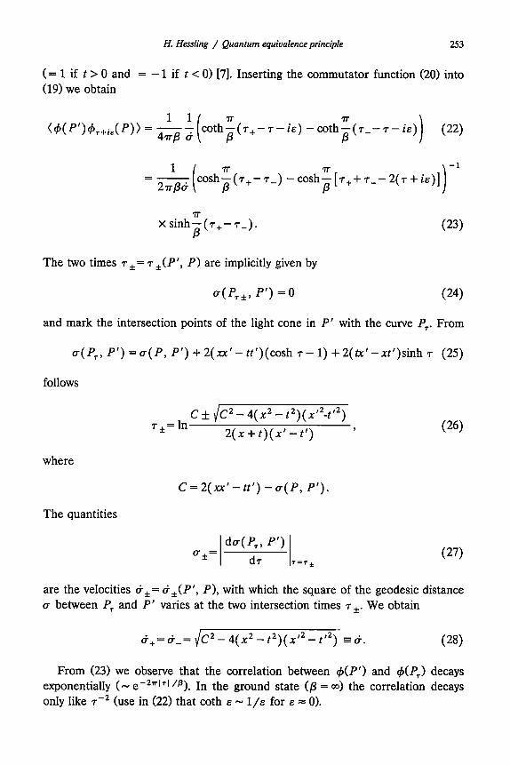
(= 1 if t > 0 and = - 1 if t < 0) [7]. Inserting the commutator function (20) into (19) we obtain

cothz(T+-A) -cothz(r-(7_-A) p P (22)

cosh;(T+-T-) -co~h~[~++7_--2(7+i&)] -1

xsinhy(r+-r-). P

(23)

The two times 7 *= 7 *(P’, P) are implicitly given by

a(P,*, P’) = 0 (24)

and mark the intersection points of the light cone in P’ with the curve PT. From

o(P7, P’) =m(P, P’) +2( xx’-ttt’)(cosh r- 1) +2(&‘-xt’)sinh r (25)

follows

r*=ln Cf\/C2- 4(x2 - t2)( d2-tt2)

2(x+t)(x’-t’) ’

where

C=2(xx’-tt’) -a(P, P’).

The quantities

(26)

(27)

are the velocities &*t= &,(P’, PI, with which the square of the geodesic distance (T between P, and P’ varies at the two intersection times T*. We obtain

&+=&-_z c”-4(g-p)(p-p) E&. (28)

From (23) we observe that the correlation between 4(P’) and c$(P,) decays exponentially ( - e- 2rr171/@). In the ground state (p = 03) the correlation decays only like rm2 (use in (22) that coth E - l/c for E J 0).


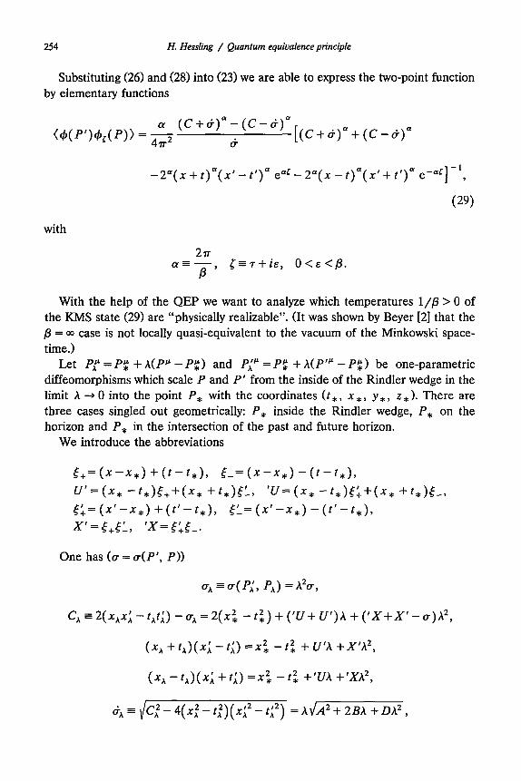
Substituting (26) and (28) into (23) we are able to express the two-point function by elementary functions

with

With the help of the QEP we want to analyze which temperatures l/p > 0 of the KMS state (29) are “physically realizable”. (It was shown by Beyer [2] that the p = co case is not locally quasi-equivalent to the vacuum of the Minkowski spacetime.)

Let Pf = P$ + A(P* - P$) and Pip = P$ + h(P” - P$) be one-parametric diffeomorphisms which scale P and P’ from the inside of the Rindler wedge in the limit A --) 0 into the point P, with the coordinates (t*, x *, y,, z, 1. There are three cases singled out geometrically: P, inside the Rindler wedge, P, on the horizon and P, in the intersection of the past and future horizon.

We introduce the abbreviations

5+=(x-x*)+(r-f*), s-=(x-x*>-(r-t*>> U’= (x* -t,)5++(~, +r*)tL, ‘U=(x* -b&5:+(x* +bX-y

g= (X)--X*) +(r’-r,), g= (x’-x*) - (r’-r*>, X’=[+c$L, ‘X=cQ-.

One has (a = dP’, PI>

u*=c-l(P,‘, P*) =A%,

CA = 2(x*x; - rhr;) - o;, = 2(x”, - r’*) + (‘U+ U’)A + (‘X+X’- 0)A2,

(xA+rA)(x;--r;) =x2, -r’, +U’h +X’h2,

(x* - rh)( x; + r;) =x: - r’, +‘UA +‘XA2,

&A~ Cf-4(x~-rj)(x;2-r;2) =A\lA2+2BA+DA2,

H. Hessling / Quantum equivalence principle

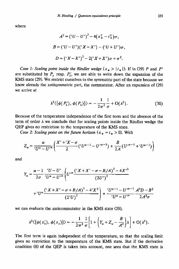
where

255

A2= (‘U- uy2 - 4(x2, -@a,

B = (‘U- U’)(‘X-X’) - (‘u+ U’)u,

D = (‘X-X’)” - 2(‘X+X’)a+a2.

Case 1: Scaling point inside the Rindler wedge (x * > 1 t * 1). If in (29) P and P’ are substituted by PA resp. Pi, we are able to write down the expansion of the Kh4S state (29). We restrict ourselves to the symmetric part of the state because we know already the antisymmetric part, the commutator. After an expansion of (29) we arrive at

~2({4(p,‘), WJ) = - ;; +0(ti2). (30)

Because of the temperature independence of the first term and the absence of the term of order h we conclude that for scaling points inside the Rindler wedge the QEP gives no restriction to the temperature of the KMS state.

Case 2: Scaling point on the future horizon (x * = t * > 0). With

z,= ff i X’+‘X-u

‘UU - U’” 2 px-l _ y-1) ; 2”, (p-l +‘u”-l))

and

a-l 'U-U' Y, = -

2a ‘LP- U’” i

u,“(~x+x’-cT-B/A)~-4x’z

(2u’)2

+,u~(‘x+x’-o.+B/A)~-4’x~ t,T,Ct-1 _ UN-1 A2D -82

(2’u)2 + ‘UU - u’* 2A2a

we can evaluate the anticommutator in the KMS state (291,

A2({4(x& 4(x*)}>= -g l+ y,+z.--$)A] +o(A2). 1 ( The first term is again independent of the temperature, so that the scaling limit gives no restriction to the temperature of the KMS state. But if the derivative condition (8) of the QEP is taken into account, one sees that the KMS state is

256 H. Hessling / Quantum equiualence principle

constant up to first order only if the coefficient of the term of order A vanishes for all P’, P in the Rindler wedge,

Y,+Z,-B/A2=0. (31)

This, in turn, is only possible if a! = 27r/P = 1, as we shall see immediately, and consequently the KMS state has the temperature l/p = 1/27r. This is the Hawk- ing-Bisognano-Wichmann temperature [l&3,4].

To solve eq. (31) is equivalent to determining cy, which solves the equation (E = (x + t - 2t*)/2t*, E’=W+t’-2t,)/2t,)

~[$A(cT+~AE$) .,A(,+E,$) +A;;;2 -B

CY-1 =-A(v2AE;) -,A(,-EA;) + A2&--B2 -B

2 (32)

for all P’, P in the Rindler wedge. Since this equation cannot be solved in closed form, we use the following trick. If the points P = (t, x0 + 5, y, z), P’ = (t’, x0 + [‘, y’, z’) are far away from the edge of the Rindler wedge, i.e. x0 z+ 15 1, 15’1, 1 t 1, 1 t’ I, we are able to bring down the exponent (Y in (32): (U’/ ‘UY = 1 + CYS with 161 = I(‘-t’-t+tl/ xc -=K 1. Thus, in the far away limit, (32) is reduced to (a - 116 + O(S2> = 0. From this follows a = 1, as claimed.

Case 3: Scaling point in the intersection of future and past horizon (x .+ = t * = 0). The scaled two-point function (29) is independent of the scaling parameter A,

A2+b(P,‘)> WA)))

a 1 (x~+‘x-u+~)“-(x’+‘x-u-~)a =-- 2a2 ti (X’+‘X-0.+~)m+(X’+‘X-u-&7)a-2aX~a-2a~X~*

According to the continuity part of the QEP the scaling limit of the right hand side has to connect continuously with the scaling limit inside the Rindler wedge. The right hand side has to be - 1/27r2a, the value given by (30). By repeating the trick of case 2 one can show that continuity is only possible if (Y = 1 resp. p = 2~.

Let use summarize: in the Rindler wedge only the KMS state with the Hawk- ing-Bisognano-Wichmann temperature is allowed by the QEP. If the scaling point is in the intersection of the future and past horizon it is sufficient to require that the scaling limit of the KMS state depends continuously on the scaling point P, in order to fix the temperature. This shows that in this case the PLS can be replaced by the continuity requirement of the QEP. If the scaling point is on the horizon a unique temperature is singled out only by the QEP and not by the PLS.


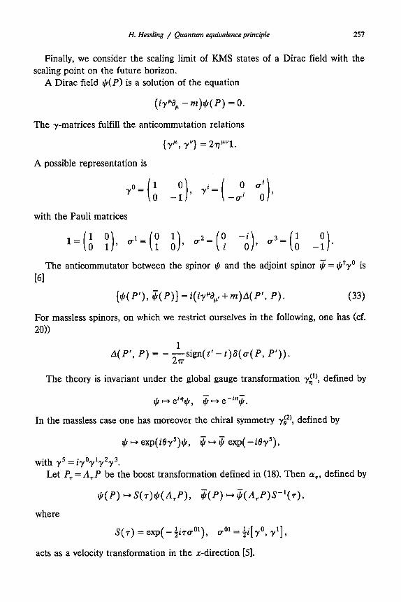
Finally, we consider the scaling limit of KMS states of a Dirac field with the scaling point on the future horizon.

A Dirac field t,NP) is a solution of the equation

(‘y”a, - m)l)( P) = 0.

The y-matrices fulfill the anticommutation relations

{y”, y”} = 27yl.

A possible representation is

with the Pauli matrices

The anticommutator between the spinor I/J and the adjoint spinor 3 = $+-y” is M

{$(P’), i.j(P)} =i(iy’“a,~+m)A(P’, P). (33)

For massless spinors, on which we restrict ourselves in the following, one has (cf. 20))

A(P’, P) = -&sign(t’-f)a(o(P, P’)).

The theory is invariant under the global gauge transformation rq), defined by

* H e’?*, $ +b e-‘“t-j.

In the massless case one has moreover the chiral symmetry yi2), defined by

J, H w(W)+, JI- $ exp( -W),

with y5 = iy”y’y2y3. Let P, = A,P be the boost transformation defined in (18). Then CY~, defined by

$(P) +qT)1(l(A,P), 6(P) +-44qw4,

where

S(T) = exp( - +aol), ~7’~ = $i[ y”, yl] ,

acts as a velocity transformation in the x-direction [S].

258 H. Hessiing / Quantum equivalence principle

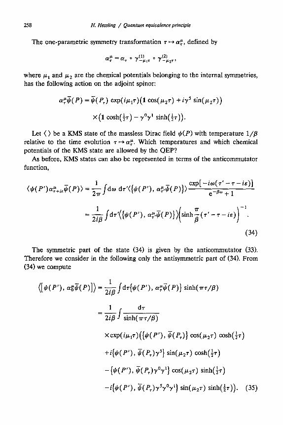
The one-parametric symmetry transformation r H CI$, defined by

where pu, and p2 are the chemical potentials belonging to the internal symmetries, has the following action on the adjoint spinor:

a)$( P) = ij( P,) exp( ipp)(l cos( p27) -I- iy’ sin( p27))

x (1 cosh( $r) - y”yl sinh( $)) .

Let ( > be a KMS state of the massless Dirac field I,@> with temperature l//3 relative to the time evolution r r--) (Y $‘. Which temperatures and which chemical potentials of the KMS state are allowed by the QEP?

As before, KMS states can also be represented in terms of the anticommutator function,

(+CP’laF+ie g(P)) = &Id, dT’({+( f”), c+?(P)}> exp[ -iw( 7’ - 7 - is)]

emPm + 1

= -&d’.({$(P.), n$$(P)})(sinhi(r’-r-k))-‘.

The symmetric part of the state (34) is given by the anticommutator (33). Therefore we consider in the following only the antisymmetric part of (34). From (34) we compute

cC$(P)} sinh(rT/P)

1 =-

/ dr

Z/3 sinh( rrr/p)

xexp(iw)({~(pr), Jlw} COS(W) =‘Sh(iT)

+i{$( P’), s( P,)y5} sin( p2T) cd($)

-{‘h(p’), ?(P,)Y”Y’} COs(k‘zT) sinh(;T)

-i{t,b(P’), $(P,)$r’r’} Sin(&T) sinh(+)). (35)


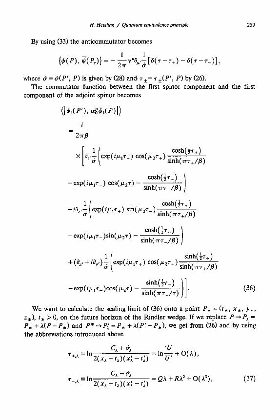
By using (33) the anticommutator becomes

where C? = N”, P) is given by (28) and 7 *= 7 *(P’, P) by (26). The commutator function between the first spinor component and the first

component of the adjoint spinor becomes

cosh( ;r+)

sinh( VT+/@)

- eXp( Zj.LIT-) cOS( &T) - cosh( +r-)

sinh( TT-//I)

cosh( $-+) sinh( ?rr+/p)

- exp( iw,r-)sin( p27) - cosh( $r-)

sinh( ?rr-/p)

sinh( $+) exp(i’lT+) COS(cL*‘+) sinh(~T+/P)

-exp( i&T-)cos( &T) - sinh( $-)

Sinh( ,T-/T) ’ (36)

We want to calculate the scaling limit of (36) onto a point P, = (t *, x *, y *, z * ), t, > 0, on the future horizon of the Rindler wedge. If we replace P + P,, = P, +A(P-P,) and P*-,P,‘=P, +A(P’-P,), we get from (26) and by using the abbreviations introduced above

c, + (;h 7 +,h = In

2(x, + t*)(xi - 0 =ln$+o(*),

c, - c;h T- ,* = In

2(x* +tn>(-d -a =Qh+Rh2+O(A3), (37)

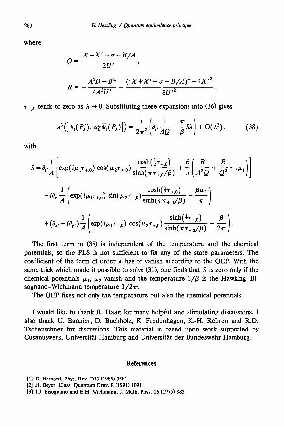
260 H. Hesling / Quantum equivalence principle

where

Q= ‘X-Xl-u-B/A

2U’ ’

A2D - B2 R=-

(‘X+X’-a-B/A)2-4X’2

4A3U’ - 8u’2

T-,~ tends to zero as A + 0. Substituting these expansions into (36) gives

h3([&(Ph)), &,(p,)]) = $(a,#& + is”) + W2). (38) with

eWlw+,ll) CO~(P27+,cl) coSh(h-+,o) +

sinW=+,dP)

- ia,.: exp(iw+.d sin(~2T+.o) i cosh(;T+.o) Pluz -- Sinh(vT+,dP) r

The first term in (38) is independent of the temperature and the chemical potentials, so the PIS is not sufficient to fix any of the state parameters. The coefficient of the term of order A has to vanish according to the QEP. With the same trick which made it possible to solve (311, one finds that S is zero only if the chemical potentials ,ur, p2 vanish and the temperature l/p is the Hawking-Bi- sognano-Wichrnann temperature 1/2~.

The QEP fixes not only the temperature but also the chemical potentials.

I would like to thank R. Haag for many helpful and stimulating discussions. I also thank U. Bannier, D. Buchholz, K. Fredenhagen, K.-H. Rehren and R.D. Tscheuschner for discussions. This material is based upon work supported by Cusanuswerk, Universitat Hamburg and Universitiit der Bundeswehr Hamburg.

References

[l] D. Bernard, Phys. Rev. D33 (1986) 3581 [2] H. Beyer, Class. Quantum Grav. 8 (1991) 1091 [3] J.J. Bisognano and E.H. Wichmann, J. Math. Phys. 16 (1975) 985

H. Hess&g / Quantum equivalence principle 261

[4] J.J. Bisognano and E.H. Wichmann, J. Math. Phys. 17 (1976) 303 [S] J.D. Bjorken and SD. Drell, Relativistic quantum mechanism (McGraw-Hill, New York, 1964) [6] J.D. Bjorken and SD. Drell, Relativistic quantum fields (McGraw-Hill, New York, 1965) [7] N.N. Bogolubov and D.V. Shirkov, Introduction to the theory of quantized fields (Interscience,

London, 1959) [S] 0. Bratteli and D.W. Robinson, Operator algebras and quantum statistical mechanics, Vol. II

(Springer, New York, 1981) [9] J.C. Collins, Renormalization (Cambridge U.P. Cambridge, 1984)

[lo] B.S. Dewitt and R.W. Brehme, Ann. Phys. 9 (1961) 220 [ll] K. Fredenhagen and R. Haag, Commun. Math. Phys. 108 (1987) 91 [12] R. Haag, N.M. Hugenholtz and M. Winnink, Commun. Math. Phys. 5 (1967) 215 [13] R. Haag, H. Namhofer and U. Stein, Commun. Math. Phys. 94 (1984) 219 [14] R. Haag, Local quantum physics (Springer, Berlin, 1992) [15] S.W. Hawking, Commun. Math. Phys. 43 (1975) 199 [16] R. Kubo, J. Math. Sot. Jpn 12 (1957) 570 1171 Ch. Lhders and J.E. Roberts, Commun. Math. Phys. 134 (1990) 29 [18] P.C. Martin and J. Schwinger, Phys. Rev. 115 (1959) 1342 [19] G. Mihalache, KMS states for Dirac quantum field in Rindler spacetime, preprint DESY 91-116

(1991) [20] L.H. Ryder, Quantum field theory (Cambridge U.P. Cambridge, 1985) [21] R. Verch, Local definiteness, primarity and quasiquivalence of quasifree Hadamard quantum

states in curved spacetime, Berlin preprint SFB-288-32 (19921, to appear in Commun. Math. Phys. [22] M. Castagnino, A. Foussats, R. Laura and 0. Zandron, Nuovo Cimento 60A (1980) 138

on the quantum equivalence principle · physics b on the quantum equivalence principle ... only the...

Documents