On the Plastic Wave Propagation Along the SpecimenLength in SHPB Test

Z.G. Wang & L.W. Meyer

Received: 20 May 2009 /Accepted: 7 September 2009 /Published online: 2 October 2009# The Author(s) 2009. This article is published with open access at Springerlink.com

Abstract To observe the plastic wave propagation, anexperimental setup is designed with a SHPB facility and ahigh speed digital camera. Two types of OFHC copper wereselected as specimen materials: in the cold work conditionand after total annealing, which represent non strainhardening and strain hardening material respectively. Therise time of incident impulse in the SHPB test is relevant tobar’s radius. A maximum allowable specimen length and amaximum allowable impact velocity (MAIV) of striker areproposed for the SHPB test. The propagation of plasticwaves is observed along specimen length at the beginningof specimen’s plastic deformation in SHPB test. However,for both types of material, no plastic wave motion is caughtalong specimen length for large plastic strain level. Sideconfinement effect of friction is found to be significant,even with lubricant in the experiment.

Keywords Split Hopkinson pressure bar (SHPB) .

Plastic wave . Equilibrium . Specimen’s geometry .

Impact velocity . OFHC copper

Introduction

It is becoming more and more important to understand themechanical behavior of materials under external high rateloading in industrial application and scientific research.

Experimentally, after Hopkinson and Kolsky’s early work[1–6], the Split Hopkinson pressure bar (SHPB) graduallybecame a widely accepted facility to test materials’mechanical properties under dynamic loading at the strainrate of 103–104/s in modern mechanical laboratory [7–12].The SHPB setup usually consists of striker, incident bar andtransmitted bars, which are all the same diameter cylindricalbars, made from hard materials. In the test, the specimen issandwiched between the incident and transmitted bars, thenthe striker hits the end of incident bar in the axial directionwith an initial velocity V. A trapezoidal incident stressimpulse is generated and propagates down the incident bar.When the length of striker is short compared with the totallength of incident bar and transmitted bar:

s i ¼ 1

2rbarcbarV ð1Þ

And the duration of the created stress impulse is:

Δt ¼ 2Lscbar

ð2Þ

Where ρbar is mass density of the bar; cbar ¼ffiffiffiffiffiffiffiffiffiffiffiffiffiffiffiffiffiffiEbar=rbar

pis the elastic longitudinal stress wave velocity in the bar;Ebar is the Young’s modulus of the bar; V is the velocity ofstriker; Ls is the length of the striker.

In laboratory application, if the Young’s modulus of thebar is known, experimenters usually can determine if thegenerated experimental incident impact pulse is goodquality or not, by calculating out the velocity and lengthof the striker from the recorded incident impulse. Thegenerated elastic stress pulse then propagates along theincident bar with the longitudinal elastic wave velocity.Transmitted and reflected stress pulses are generated and

Z.G. Wang (*) : L.W. MeyerInstitute of Material and Impact Engineering Laboratory,Faculty of Mechanical Engineering and Processing,Chemnitz University of Technology,09107 Chemnitz, Germanye-mail: wangzonggang@gmail.comURL: www.wsk.tu-chemnitz.de

Experimental Mechanics (2010) 50:1061–1074DOI 10.1007/s11340-009-9294-x

propagated in the transmitted bar and incident bar respec-tively, when the incident impulse loads the specimen. Whenthere is force equilibrium between the specimen’s incidentand transmitted sides (relationship of incident, reflected andtransmitted signals is equation (3)), the specimen isuniformly deformed, and the stress-strain curves of thematerial can be determined with one dimensional assumptionfrom equations (4) and (5):

"t ¼ "i þ "r ð3Þ

s ¼ AbarEbar"tAsp

ð4Þ

": ¼ 2cbar"r

Lð5Þ

where εt, εi and εr are the values of transmitted, incidentand reflected signals in the bars respectively; �" is theloading strain rate of the tested specimen; L is the initiallength of the tested specimen.

If there is no force equilibrium for the two sides ofspecimen in the SHPB test, it means the measurement isuncertain and no calculation can be done from the recordedsignals, using the above equations. So generally in theSHPB test, the specimen is dynamically and uniformlydeformed, the only difference between quasi-static test andso-called dynamic test in the SHPB test is deforming rate(i. e. strain rate).

The above classic analysis of SHPB test is widelyapplied by experimenters to determine the mechanicalbehavior of tested materials under dynamic loading.Scientists try to increase the striker’s velocity and reducethe specimen’s dimension, as far as they can, to get higherstrain rate loading on the specimen [13].

However, the above data processing method for theSHPB test is based on two assumptions: one is forceequilibrium on both sides of the specimen, the other is theone dimensional uniformly deformed specimen. About theforce equilibrium, to minimize experimental errors, one canimprove the recorded strain gage signals by applyingexperimental techniques, such as keeping good contactbetween bars and specimen, reducing the friction betweenbars and supporters, keeping bars well coaxial and so on.But is the specimen really one dimensional uniformlydeformed in SHPB test as a quasi-static test? In the quasi-static test, the specimen is deformed at a very low strainrate (10−3/s), so loading stress waves have sufficient time topass and reflect along the specimen length and the onedimensional assumption can be easily satisfied. On the

other hand, in SHPB test, no matter what the specimen’smaterial is and what the specimen geometry is, initially thestress waves will always travel along the specimen from theincident side to the transmitted side, at a velocitycomparable to that of the loading. As we know, the elasticlongitudinal wave velocity in solids is around 4,000–5,000 m/s, so for a specimen with 5–10 mm length, thestress wave can pass it in 1 μs or 2 μs, if the stress wavestravel along the specimen length with the elastic longitudinalwave velocity for the whole loading time. So comparing withthe hundred-microsecond loading time of the incidentimpulse, this passing time along specimen length of the stresswaves is sufficiently short, and the specimen can be uniformlyone dimensionally deformed as in the quasi-static test.

However, plastic wave theory was proposed and developedin 1950’s [14–16]. In the theory, stress waves propagate inthe medium with the velocity, which is related to the slope ofmaterial’s true stress-strain curve (modulus E) and massdensity. In equation (6), modulus E can be either the elasticYoung’s modulus or the plastic modulus respectively, whenthe material is elastically or plastically deformed:

E ¼ @s true

@"trueð6Þ

As shown in Fig. 1, for a specific material, the plasticmodulus is much smaller than the elastic modulus. Thus,when specimen undergoes plastic deformation, the stresswave velocity will be significantly slower, especially fornon strain hardening materials. So in an SHPB test, the timefor the stress wave passing and reflecting the specimenlength and building up force equilibrium maybe can’t be

0 0.02 0.04 0.06 0.08 0.10

0.5

1

1.5

2

2.5

3

3.5

4

4.5x 10

8

TRUE STRAIN

TR

UE

ST

RE

SS

[Pa

]

ELASTIC MODULUS Ee

PLASTIC MODULUS Ep

Fig. 1 A stress-strain diagram to show a material’s different Moduliin the elastic and plastic deformation domain

1062 Exp Mech (2010) 50:1061–1074

treated as short (compared with dynamic loading time),which might lead to a non-uniform deformation along thespecimen length and do not fulfill the equilibrium conditionat the beginning of specimen’s plastic deformation in theSHPB test.

Here, by taking account into plastic wave propagationeffect, we’ll investigate the data processing method of theSHPB test again and try to determine the technique andspecimen geometry limitations in the SHPB test. After-wards, an experimental setup is built with a SHPB systemand a high speed digital camera to experimentally observethe plastic wave propagation along specimen length duringdynamic loading. Then a virtual SHPB setup is numericallymodeled by commercial software to authenticate andexplain the theoretical results. In the end, discussion andconclusion are made to interpret newly developed results.

Theoretical Analysis

In SHPB test, when the striker hits the incident bar in theaxial direction, a trapezoidal stress impulse is generated andthen propagates along the incident bar (Fig. 2). From anelastic wave analysis point of view, what composes theincident impulse and what the strain gages on the bar canrecord are the stress wave components with a longitudeelastic velocity

ffiffiffiffiffiffiffiffiffiffiffiffiffiffiffiffiffiffiEbar=rbar

pin the axial direction. Kolsky

and Davies did full frequency analysis on elastic stresswave propagation in SHPB test by using the Pochhammerand Chree equations [17–21], which can successfullydescribe such wave motions in an elastic cylindricalmedium [2, 3]. They concluded that wave components,

which propagate along the bar with the elastic wavevelocity

ffiffiffiffiffiffiffiffiffiffiffiffiffiffiffiffiffiffiEbar=rbar

p, are only those with long wave lengths

r=Λ < 0:1 (i.e. lower frequencies. Λ is wave length; ris the radius of bar) [2, 3]. So when the incident stressimpulse travels along the elastic cylindrical bar, it’sdistorted and dissipated. Finally, what strain gages recordand what loads are applied to the specimen are only thosewave components with long wave lengths. All other wavecomponents with short wave lengths or high frequencies arefiltered out.

In addition, from linear frequency analysis theory, for astep signal with a rising time Tr and a duration time Δt(shown in Fig. 3), we have the following relationship:

Tr � Tmin=2 ð7Þ

Tmax � Δt=2 ð8Þ

where Tmin and Tmax are the minimum and maximumperiod of wave components in the signal respectively. So byapplying the above linear wave analysis result, the incidentimpulse has following properties:

Wave lengthwindow: 10r < Λ < 4Ls ð9Þ

Periodwindow:10r

cbar< T <

4Lscbar

ð10Þ

Frequencywindow:p2Ls

< w <p5r

ð11Þ

And the rise time of incident impulse is around:

Tr � 5r

cbarð12Þ

From equation (12), for the 19.7 mm diameter steelSHPB system in the Material and Impact EngineeringLaboratory of the Faculty of Mechanical EngineeringChemnitz University of Technology, the rise time of theincident impulse should be: Tr � 11ms. By contrast, atypical experimental incident signal recorded by straingages is shown in Fig. 4, of which Tr is about 12 μs. Theexperimental results match the theoretical analysis verywell.

It’s widely accepted that force equilibrium on thespecimen in SHPB test is established in this rising time

0 1 2 3 4

x 10-4

-0.05

0

0.05

0.1

0.15

0.2

0.25

0.3

TIME [S]

ST

RA

IN

t

Fig. 2 The incident stress impulse recorded by strain gages on theincident bar in SHPB test [the amplitude and time duration can becalculated by equations (1) and (2) respectively]

Exp Mech (2010) 50:1061–1074 1063

duration. So a maximum allowable specimen length isobtained:

Lmax ¼ 1

n

cspcbar

5r � 5r

nð13Þ

where csp is the elastic wave velocity in specimen; n is thenumber of times stress waves travel along the specimen’slength, to build the force equilibrium, which is believed tobe three or four times.

Once force equilibrium is established, equations (3), (4)and (5) are immediately valid. When the specimen’sdeformation is just passing the yield point of the specimen’smaterial, the following classic relationship is satisfied fromone dimensional Hooke’s law:

sy ¼ Esp"y ð14Þ

sy and Esp are the yield stress and Young’s modulus of thespecimen respectively.

At the yield point, if the strain rate �" is known, theloading time on the specimen can be calculated as:

ty ¼ sy

Esp�" ð15Þ

From Von Karman’s plastic wave theory, the velocity ofthe stress wave will immediately reduce from the elasticwave velocity to the plastic wave velocity, when thespecimen yields and starts plastically deforming. So inthe time duration ty, the stress wave at least has to pass thewhole specimen and reach the transmitted side of the

specimen. The specimen length should fulfill the followingequation:

L � cspty ð16Þ

Now applying the data processing method of SHPB andsubstituting equations (3), (5) and (15) into the aboveequation, we have:

cspsy

2cbarEsp "i � "tð Þ �L

L¼ 1 ð17Þ

From equation (4), when the specimen is yielding, thetransmitted signal obeys the following relationship:

"t ¼ Asp

AbarEbarsy ð18Þ

Furthermore, from one-dimensional Hooke’s law andequation (1), the strain of the incident impulse is:

"i ¼ rbarcbarV2Ebar

ð19Þ

Substituting equations (18), (19) into equation (17), anddoing simplification and rearrangement, we obtain:

V � 1

2

rbarcbarrspcsp

þ d2spd2bar

!2sy

rbarcbarð20Þ

where dsp and dbar are diameter of the specimen and barrespectively.

0.9 1 1.1 1.2 1.3 1.4

x 10-4

0

0.05

0.1

0.15

0.2

0.25

0.3

TIME [s]

ST

RA

IN F

RO

M S

TR

AIN

GA

GE

S

Tr

Fig. 4 An incident impulse measured by strain gages on the incidentbar of the 19.7 mm diameter SHPB facility in our laboratory

0 1 2 3 4 50

1

TIME

SIG

NA

L

Tr

t

Fig. 3 A step signal with a rising time Tr and a duration time Δt

1064 Exp Mech (2010) 50:1061–1074

Now in equation (20), there are only material constantsof specimen and bar in the right hand. Let

C1 ¼ 1

2

rbarcbarrspcsp

ð21Þ

C2 ¼d2spd2bar

ð22Þ

Finally we have:

V � C1 þ C2ð Þ 2sy

rbarcbarð23Þ

Equation (23) shows there is a maximum allowableimpact velocity (MAIV) of striker in the SHPB test. When

the striker’s velocity is lower than MAIV, the condition forbuilding up force equilibrium is fulfilled; so the specimencan be uniformly deformed in the SHPB test. On the otherhand, if the striker’s velocity is higher than MAIV, incidentside of specimen is always plastically deformed before thetransmitted side of specimen yields; i.e. the specimenundergoes non-uniform plastic deformation, which maylead to the SHPB experiment being invalid.

In equation (23), both C1 and C2 are dimensionlessparameters and have clear physical meaning. C1 representsthe relative material property ρc, and C2 is the square ofdiameter ratio of specimen and bar, which describes thespecimen’s relative geometrical dimension in one specificSHPB test. In addition, MAIV is proportional to the yieldstress of the specimen material, which means MAIV will berather low, if the test specimen’s yield stress is too low. Forfurther discussion, relevant mechanical properties of the19.7 mm diameter steel SHPB system in our Laboratory andseveral selected common engineering alloys are presented inTable 1.

Figure 5 shows the variation of MAIV as a function ofthe specimen’ normalized diameter by that of the bar dsp/dbar. Since normally the specimen’s diameter is smaller thanthat of the bar, the value of C2 should vary from zero to 1.In the figure, for soft materials (low yield and plastic flow

Material Young’s modulus[GPa]

Mass density[kg/m3]

Longitude wavevelocity [m/s]

Yieldingstress [MPa]

Steel 181.5 7970 4772 2000

Tungsten 380 19300 4437 1700

Ti6Al4V 113.8 4430 5068 970

Al6063 69 2700 5055 300

Mg AM50 45 1770 5042 110

OFHC copper 110 8960 3503 30/320

Table 1 Mechanical constantsof selected typical engineeringmaterials

0 0.2 0.4 0.6 0.8 10

10

20

30

40

50

60

70

80

NORMALIZED SPECIMEN DIAMETER BY BAR

MA

XIM

UM

ALL

OW

AB

LE V

ELO

CIT

Y [m

/s]

TungstenTi6Al4VAl6063

Mg AM50OFHC Copper aaOFHC Copper cwc

Fig. 5 MAIV changes as a function of normalized specimen’sdiameter, which is equal to dsp/dbar for several typical engineeringmaterials (OFHC copper aa means after annealing; OFHC copper cwcmeans in a cold work condition)

Fig. 6 An OFHC copper specimen with a white background andblack dot pigment surface before the test

Exp Mech (2010) 50:1061–1074 1065

stress compared with bar material): e. g. MgAM50, Al6063,and OFHC copper, MAIV isn’t sensitive to the variation ofspecimen diameter. Yield stress of the tested materialbecomes a dominant parameter, for example, the MAIVfor OFHC copper after total annealing is only around 1 m/sto 2 m/s, which corresponds to a rather low yield stress30 MPa. So it becomes quite understandable that very softmaterials aren’t suitable for SHPB test because of theirlow yield stresses, no matter what the specimen geometryis. On the other hand, for hard materials (comparedwith bar material): Tungsten and Ti6Al4V, for which thevalue of ρc is equivalent to hard steel, thus, relativegeometrical parameter becomes significant for MAIV.MAIV increases significantly with specimen diameter.MAIV varies from 20 m/s to 100 m/s for Tungsten andfrom 40 m /s to 90 m/s for Ti6Al4V. In such case specimendiameter becomes critical in the SHPB test and should becarefully chosen.

Experimental Observation

The 19.7 mm diameter SHPB in our laboratory was used toobserve plastic wave propagation along specimens using ahigh speed digital camera (REDLAKEHGK100), which has a50 µs frame rate and is assembled to focus on the specimen’shalf cylindrical surface during the test. According to the abovetheoretical analysis and because of its low plastic wavevelocity [16, 22, 23], OFHC copper was selected asexperimental specimen material. The specimen geometrywas chosen as 10–20 (mm) diameter-length cylinder. In thetest, the specimen cylindrical surface was covered by a thinlayer of white background and black dot pigments (shown inFig. 6).

Both the oscilloscope for the strain gages on the bars andthe camera are triggered by 5% increasing incident strainimpulse and a software post trigger was also designed forthe camera to enhance the camera’s frame resolution. Sohalf full cylindrical surface photographs of the experimentalspecimen can be recorded simultaneously with the strainsignals from the SHPB test, and half cylindrical strain fieldcan be obtained from the photographs afterwards by anoptical deformation and strain measurement software:ARAMIS V6.0.1-3, which is an optical technique tomeasure the deformation and strain of the surface ofspecimen and can recognize the surface structure of themeasuring object in digital camera images and allocatescoordinates to the image pixels.

The OFHC copper specimens are classified to two groups:as received in a cold work condition and after total annealingheat treatment. Static true stress-strain curves for these twotypes of OFHC copper specimens are shown in Fig. 7, andnecessary technique coefficients for specimen and trigger inthe experiment are shown in Table 2. For the OFHC copperspecimens in the cold work condition, yield stress is around300 M Pa and plastic stress almost remains constantregardless of plastic strain level, which is a typical non-

0 0.05 0.1 0.15 0.2 0.25 0.3 0.350

0.5

1

1.5

2

2.5

3

3.5x 10

8

TRUE STRAIN

TR

UE

ST

RE

SS

[Pa

]

IN A COLD WORK CONDITIONAFTER HEAT TREATMENT

Fig. 7 Static stress-strain curves of OFHC copper specimens in a coldwork condition and after total annealing

Specimen Material Diameter/length[mm/mm]

Triggerlevel [mV]

Post trigger timeof the camera [μs]

#1 Cold work condition 10/20 638 0

#2 Cold work condition 10/20 638 10

#3 Cold work condition 10/20 638 20

#4 Cold work condition 10/20 638 30

#5 Cold work condition 10/20 638 40

#6 After annealing 10/20 638 0

#7 After annealing 10/20 638 10

#8 After annealing 10/20 638 20

#9 After annealing 10/20 638 30

#10 After annealing 10/20 638 40

Table 2 Technique data ofOFHC copper specimens andtriggers in the SHPB test withcamera

1066 Exp Mech (2010) 50:1061–1074

strain hardening material and may lead to a very low plasticwave velocity (especially at the large plastic strain level)from Von Karman’s one dimensional plastic wave theory. Bycontrast, the OFHC copper specimens after total annealingheat treatment have a very low yield stress 30 M Pa andplastic stress increases with plastic strain level, which is atypical strain hardening material. The strain hardening effectis significant and plastic wave velocity reduces from theelastic value more moderately than OFHC copper specimensin the cold work condition, once specimen starts plasticdeformation. For these two types of OFHC copper, theoreticalplastic wave velocities, calculated from Von Karman’s theory,are shown in Fig. 8.

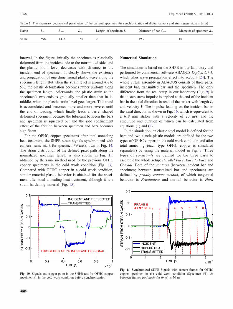
A schematic of the SHPB in our laboratory is shown inFig. 9 and necessary parameters are shown in Table 3 tosynchronize the photograph frames of the camera and thestrain gage signals. By keeping the camera time scale static,and moving the strain gage signals recorded from the bars,we can synchronize the results from the camera and straingage signals of the SHPB as:

Tincid ¼ Ttrig þ Lbar�2cbar � Tp trig ð24Þ

Trefl ¼ Ttrig � Lbar�2cbar � Tp trig ð25Þ

Ttrans ¼ Ttrig � Lsg�cbar � Tp trig � L

�csp ð26Þ

Where, Tincid, Trefl and Ttrans are the time duration to beshifted for those signals respectively; Tp_trig is the camera’spost trigger time. As an example, Figs. 10 and 11 show therecorded and shifted (with the mark of camera frames)SHPB signals of specimen #1 respectively. The halfcylindrical strain fields of specimen #1 are shown inFig. 12 with a 50 µs time step, which are obtained fromphotographs after imaging processing using softwareARAMIS V6.0.1-3. In the software, the half cylindricalsurface of the specimen is divided into 10 × 20 pixels, i. e.one pixel is approximately one square millimeter [Fig. 12(a)]. As the specimen is deformed, each pixel also movesand deforms. The software can track each pixel displace-ment, calculate the deformation, and display the whole halfcylindrical strain field of the specimen. However, in theexperiment some pixels in the strain field may be missed,especially for large plastic strain levels [Fig. 12(d), (e) and(f)], because part of the pigments on the cylindrical surfacesometimes fly away during dynamic loading. Since our aimis to observe the propagation of plastic waves along thespecimen length in an SHPB test and test Von Karman’sone-dimensional plastic wave theory, the variation of strainalong the specimen length is the most interesting result. Sothe pixel path along the specimen length in the middle ofthe half cylindrical strain field is selected to represent thestrain status of specimen, to minimize error from thecamera’s depth of field.

For the OFHC copper specimens in the cold workcondition, Fig. 13 shows the strain distribution of thedefined pixel path along its normalized length. Solid curvesare from frame 3 to frame 9 of specimen #3, whichcorresponds to the red dashed-dot line in Fig. 11. As thepost trigger is designed to increase the resolution of thecamera, the corresponding results (dashed lines) of speci-mens #1, #2, #4 and #5 are inserted between the curves offrame 3 and frame 4 of specimen #3 with a 10 µs time

0 0.05 0.1 0.150

200

400

600

800

1000

TRUE STRAIN

PLA

ST

ICE

WA

VE

VE

LOC

ITY

[m/s

]

IN A COLD WORK CONDITIONAFTER TOTAL ANNEALING

Fig. 8 Theoretical one dimensional plastic wave velocities as afunction of true strain for the two type OFHC copper specimens (inthe cold work condition and after total annealing), calculated from truestress-strain curves in Fig. 7

Fig. 9 Schematic of the SHPBsetup in our laboratory ofTU-Chemnitz

Exp Mech (2010) 50:1061–1074 1067

interval. In the figure, initially the specimen is plasticallydeformed from the incident side to the transmitted side, andthe plastic strain level decreases with distance to theincident end of specimen. It clearly shows the existenceand propagation of one dimensional plastic wave along thespecimen length. But when the strain level is around 4% to5%, the plastic deformation becomes rather uniform alongthe specimen length. Afterwards, the plastic strain at thespecimen’s two ends is gradually smaller than that in itsmiddle, when the plastic strain level goes larger. This trendis accumulated and becomes more and more severe, untilthe end of loading, which finally leads a barrel shapeddeformed specimen, because the lubricant between the barsand specimen is squeezed out and the side confinementeffect of the friction between specimen and bars becomessignificant.

For the OFHC copper specimens after total annealingheat treatment, the SHPB strain signals synchronized withcamera frame mark for specimen #9 are shown in Fig. 14.The strain distribution of the defined pixel path along thenormalized specimen length is also shown in Fig. 15,obtained by the same method used for the previous OFHCcopper specimens in the cold work condition (Fig. 13).Compared with OFHC copper in a cold work condition,similar material plastic behavior is obtained for the speci-mens after total annealing heat treatment, although it is astrain hardening material (Fig. 15).

Numerical Simulation

The simulation is based on the SHPB in our laboratory andperformed by commercial software ABAQUS Explicit 6.7-1,which takes wave propagation effect into account [24]. Thewhole virtual assembly in ABAQUS consists of three parts:incident bar, transmitted bar and the specimen. The onlydifference from the real setup in our laboratory (Fig. 9) isthat a step stress impulse is applied at the end of the incidentbar in the axial direction instead of the striker with length Lsand velocity V. The impulse loading on the incident bar inthe axial direction is shown in Fig. 16, which is equivalent toa 618 mm striker with a velocity of 20 m/s, and theamplitude and duration of which can be calculated fromequations (1) and (2).

In the simulation, an elastic steel model is defined for thebars and two elastic-plastic models are defined for the twotypes of OFHC copper: in the cold work condition and aftertotal annealing (each type OFHC copper is simulatedseparately) by using the material model in Fig. 7. Threetypes of constraints are defined for the three parts toassemble the whole setup: Parallel Face, Face to Face andCoaxial. Both of the contacts (between incident bar andspecimen; between transmitted bar and specimen) aredefined by penalty contact method, of which tangentialbehavior is Frictionless and normal behavior is Hard

Table 3 The necessary geometrical parameters of the bar and specimen for synchronization of digital camera and strain gage signals [mm]

Name Ls Lbar Lsg Length of specimen L Diameter of bar dbar Diameter of specimen dsp

Value 598 1475 150 20 19.7 10

0 0.2 0.4 0.6 0.8 1

x 10-3

-0.2

-0.1

0

0.1

0.2

0.3

TIME [s]

ST

RA

IN F

RO

M S

TR

AIN

GA

GE

S

INCIDENT AND REFLECTEDTRANSMITTED

TRIGGERED AT 5% INCREASE OF SIGNAL

Fig. 10 Signals and trigger point in the SHPB test for OFHC copperspecimen #1 in the cold work condition before synchronization

ST

RA

INF

RO

MS

TR

AIN

GA

GE

SS

TR

AIN

FR

OM

ST

RA

IN G

AG

ES

-0.

-0.

0.

0.

0.

0

2

1

0

1

2

3

FAFRAAT 9

INRETR

AM97.

1

NCIEFRA

E 0.38

DELE

ANS

08µs

ENTECTSMI

1

TTEDTT

2

DTED

2

T

D

TIM

3

ME 3[s]

4

]

5

4

6 77 8

5

x

8

10--4

Fig. 11 Synchronized SHPB Signals with camera frames for OFHCcopper specimen in the cold work condition (Specimen #1). Δtbetween frames (red dash-dot lines) is 50 µs

1068 Exp Mech (2010) 50:1061–1074

Contact. The dimensions and technique parameters in thesimulation are given in Table 4.

Since here our task is to investigate the specimen’s plasticdeformation and the effect of plastic wave propagation, failure

of specimen’s material model wasn’t considered in thesimulation (actually these two types of OFHC copper speci-mens do not fail in the real SHPB test). On the other hand,strain rate effects on material behavior of the specimens is also

(c) Frame 5, t=347.38µs

(a) Frame 3, t=247.38µs

(e) Frame 7, t=447.38µs

(b) Frame 4, t=297.38µs

(d) Frame 6, t=397.38µs

(f) Frame 8, t=497.38µs

Fig. 12 Half cylindrical strain field of the compression specimen #1 with a 50 µs time step

1

15

20

TR

UE

ST

RA

IN [

%]

00

5

NORMALIZED PIXELS BY SPECIMEN LENGTH

0.2 0.4 0.6 0.8 1

Impact

direction

Fig. 13 The strain distributionof the pixel path along specimenlength in the cold workcondition (x axis is the pixelsnormalized by specimen’slength, it’s always from 0 to 1nevertheless specimen’s plasticdeformation level). Solid curvesare results of frame 3 to frame 9for specimen #3, of which Δt is50 µs. Dashed curves are resultsof specimen #1, #2, #4 and #5,of which Δt is 10 µs

Exp Mech (2010) 50:1061–1074 1069

ignored; i.e. strain rate hardening was not included in materialmodel for the sake of constant nominal strain rate in the SHPBtest.

To compare with results from the digital camera, a nodalpoint path (shown in Fig. 17) is also defined along thespecimen length (z axis direction) for each simulation,which corresponds to the pixel path in the previousexperimental half cylindrical strain field. The historicalplastic strain distribution in the z axis direction is recordedand plotted as normalized specimen length in Figs. 18 and19 for these two types of OFHC copper specimens with a10 µs time interval. Since numerical simulation strictlyobeys Von Karman’s plastic wave theory, there is a verylow plastic wave velocity for OFHC copper specimens in

the cold work condition (Fig. 8). So in Fig. 18, thespecimen’s deformation is quite non-uniform along itslength and the plastic strain on the specimen incident sideis always larger than that in specimen transmitted side. Thisnon-uniform strain distribution becomes more and moresevere as the strain lever becomes larger, and finally thecross section of the specimen changes from a rectangularshape to a trapezoidal shape. By contrast, there is arelatively high plastic wave velocity (400 m/s to 600 m/s)for OFHC copper specimens after total annealing heattreatment. The propagation and reflection of plastic wavesalong the specimen length are clearly shown in Fig. 19,thus the plastic strain distribution along specimen length is

0 0.2 0.4 0.6 0.8 1

x 10-3

0

0.5

1

1.5

2

2.5

3

3.5

4x 10

8

SIMULATION TIME [S]

HIS

TO

RIC

AL

LO

AD

ING

ON

INC

IDE

NT

BA

R [P

a]

Fig. 16 Compression loading on the incident bar in the numericalsimulation (note: the value should be negative, if the loading directionis taken into account)

0 1 2 3 4 5

x 10-4

-0.2

-0.1

0

0.1

0.2

0.3

TIME [s]

ST

RA

IN F

RO

M S

TR

AIN

GA

GE

S

INCIDENTREFLECTEDTRANSMITTED

2FRAME 0AT 97.38µs 1 3 85 764

Fig. 14 Synchronized SHPB Signals with camera frames for OFHCcopper specimen after total annealing (Specimen #9). Δt betweenframes (red dash-dot lines) is 50 µs

0 0.2 0.4 0.6 0.8 10

5

10

15

20

NORMALIZED PIXELS BY SPECIMEN LENGTH

TR

UE

ST

RA

IN [%

]

Impactdirection

Fig. 15 The strain distributionof the pixel path along specimenlength after total annealing heattreatment (x axis is the pixelsnormalized by specimen length,it’s always from 0 to 1nevertheless specimen’s plasticdeformation level). Solid curvesare results of frame 3 to frame 9for specimen#9, of which Δt is50 µs. Dashed curves arecorresponding results ofspecimen #6, #7, #8 and #10, ofwhich Δt is 10 µs

1070 Exp Mech (2010) 50:1061–1074

much more uniform than that for OFHC copper in the coldwork condition.

Discussion

In the first part of this paper, the incident stress impulse wasinvestigated by elastic wave frequency analysis, since thewhole procedure of its generation and propagation alongthe axial direction of the bar is totally elastic. It was foundthat rise time of the incident stress impulse is related to theradius and elastic longitudinal wave velocity of the barfrom equation (12). In real experiments, there are differ-ences between the incident stress impulse shapes fromdifferent SHPB facilities. One may think this difference isonly due to the properties of the bar material or experi-mental conditions, but we clearly show that it’s alsodominated by bar radius, which determines the highestfrequency components of elastic waves propagating alongthe bar with the elastic longitudinal velocity [2, 3, 17–21].The shape of the incident stress impulse can be improved toa nearly perfect step impulse by reducing the bar radius.Furthermore, to build the force equilibrium in this timeduration, a maximum allowable specimen length is given asa technique criterion for the SHPB test. The discussion hereabout the specimen length can explain Duwez and Clark’sresults on specimen length very well [22].

Second, the data processing method of the SHPB test isre-examined by the introduction of Von Karman’s plasticwave theory. A maximum allowable impact velocity(MAIV) for a striker is obtained as another techniquecriterion in the SHPB test. From Fig. 5, for soft testingmaterial with a low yield stress, the effect of specimendiameter/radius is small on MAIV, but the value of MAIVis also very small. In addition, the experimental techniquefor soft materials (such as rubber, human tissue.) comparedwith metal was developed by Chen [11, 26]. A standardsteel SHPB with modified techniques had to be used toinvestigate rubber specimen’s dynamic mechanical proper-ties. Although the conception of elastic Young’s modulusand yield stress aren’t appropriate parameters for these softmaterials, the above conception of MAIV also has some-thing meaningful in explaining the difficulties of the SHPBtest. Compared with bar material, the plastic flow stress ofthe soft material is far less than that of steel. So the value ofMAIV is rather small, no matter what the specimengeometry is. The plastic deformation of the incident sideof specimen always takes place earlier than that of thetransmitted side. Auxiliary facility has to be introduced toovercome the difficulty [11, 26].

Although previous results are generally based on SHPBtests in compression, MAIV can also be extended to thetension and torsion cases. Especially the SHPB tension test,sometimes, the specimen necks near the incident side at thebeginning of the dynamic loading, which is called earlynecking, when the material of specimen is rather soft.MAIV can explain such phenomenon as being mainly dueto the low yield stress of the tested material and too high animpact velocity. Furthermore, for brittle materials such asceramics with a high yield stress [25], the specimengeometry becomes a key factor for validation of the SHPBtest as well as the striker’s impact velocity.

Third, an SHPB experiment with high speed camera wasdesigned to record the plastic wave propagation along aspecimen length by using two kinds of OFHC copperspecimens: (i) in the cold work condition and (ii) after totalannealing, and whose length was longer than the theoreticalmaximum allowable length, and for which impact velocityof the striker was higher than the MAIV. From Figs. 13 and15, for both kinds of material, plastic wave propagation

Fig. 17 Defined nodal point path on specimen cylindrical surface inthe numerical simulation, which is along specimen length during thedynamic loading

Table 4 Parameters of the numerical model in the simulation

Part Material Diameter[mm]

Length[mm]

Section Elementtype

Meshsides [mm]

Incident bar Maraging 19.7 1475 Bar 3D stress 0.8

Transmitted bar Maraging 19.7 1475 Bar 3D stress 0.8

Specimen 1 OFHC copper in the cold work condition 10 20 Specimen 3D stress 0.2

Specimen 2 OFHC copper after total annealing 10 20 Specimen 3D stress 0.2

Exp Mech (2010) 50:1061–1074 1071

along specimen length (the non-uniform plastic deforma-tion) can be observed when the specimens just beganplastic deformation. As the plastic strain level increased, theplastic strain along the specimen length was rather uniform,and no motion (propagation and reflection) of plastic wavewas detected either for the strain hardening material or forthe non strain hardening material. The above experimentalresults can verify previous researchers’ observation [30–32]. When the plastic strain level became more than 10%,side confinement effect of the friction between specimenand bars became evident, which has a significant influenceon material’s behavior under dynamic loading and failuremodel [27–29].

Fourth, numerical simulation showed the plastic straindistributions along the specimen length are quite differentfor OFHC copper specimens in the two conditions. Forstrain hardening material, i. e. OFHC copper after totalannealing heat treatment, the propagation and reflection of

plastic wave along specimen length obviously existed atlarge strain, as it has a relatively high plastic wave velocity.For non strain hardening material, i.e. OFHC copper in thecold work condition, the plastic strain was rather nonuniform along the specimen length; the incident side ofspecimen always had a larger plastic strain than on thetransmitted side. These differences between experimentaland numerical results call our attention to the validation ofplastic wave theory. In fact, the theory has two fundamentalsimplifying assumptions. First there is no strain rate effectin the stress-strain behavior of the material. The other is thatthe lateral or radial motion of the material can be neglected[33]. But in the experiment, with a large plastic strainspecimen, the radial motion of the specimen can’t beneglected, so the plastic wave theory can’t be applied anymore. This is why experimental results are different fromnumerical simulation. In addition, the side confinementeffect of friction in the SHPB test makes the one

0 0.2 0.4 0.6 0.8 10

0.05

0.1

0.15

0.2

NORMALIZED NODE POINTS BY SPECIMEN LENGTHP

LAS

TIC

ST

RA

IN

Impact

direction

Fig. 18 Historical plastic strainalong specimen length direction(the nodal point path defined inFig. 17) for OFHC copperspecimen in the cold workcondition from numericalsimulation (Time betweencurves is 10 µs)

0 0.2 0.4 0.6 0.8 10

0.05

0.1

0.15

0.2

0.25

NORMALIZED NODE POINTS BY SPECIMEN LENGTH

PLA

ST

IC S

TR

AIN

Impact

direction

Fig. 19 Historical plastic strainalong specimen length direction(the nodal point path defined inFig. 17) for OFHC copperspecimen after total annealingfrom numerical simulation(Time between curves is 10 µs)

1072 Exp Mech (2010) 50:1061–1074

dimensional assumption no longer valid, which may beanother reason that Von Karman’s theory does not hold.

Here we have to mention Klepaczko’s theory of criticalimpact velocity (CIV), which is the criterion of a material’sadiabatic thermal instability under dynamic loading [34].From the above analysis, the CIV maybe is not suitable forlarge failure strain materials, since the plastic wave theoryis no longer applicable.

One may think that the non-uniform plastic straindistribution along specimen’s length, which is observed inthe SHPB test, may be from the oscillations on the incidentimpulse. But from Figs. 11 and 14, for the frame 4, whenringing has really attenuated, there is still a non uniformstrain distribution along the specimen length (Figs. 13and 15).

Conclusion

The data processing method of SHPB test is re-investigatedby introduction of plastic wave theory. An experimentalsetup is designed with a SHPB facility and a high speeddigital camera by using OFHC copper specimens in twoconditions: in the cold work condition and after totalannealing heat treatment. Numerical simulation is also doneby commercial software ABAQUS Explicit 6.7-1 as anauxiliary method to compare with experimental results. Thefollowing conclusions can be drawn:

& The rise time of an incident impulse in SHPB test isrelated to the bar’s radius/diameter and elastic longitudinalvelocity, which can be shorter by reduction of the bar’sradius/diameter;

& The maximum allowable specimen length is given as atechnique criterion of the SHPB test;

& The maximum allowable impact velocity (MAIV) ofstriker can be considered as a technique criterion for aspecific material in SHPB test;

& The propagation of plastic wave is observed alongspecimen length at the beginning of specimen’s plasticdeformation in SHPB test. However, no more wavemotions can be experimentally caught at large plasticstrain levels, whether the specimen material strainhardens or not. Plastic wave theory is experimentallyproved to be only valid at low plastic strain level.

& Side confinement effect of friction between bars andspecimen may play an important role for material’sbehavior under dynamic loading in the case of largeplastic strain, even if lubricant is used.

Acknowledgements This work was supported by DFG through agrant ME 1457/12-3 to Prof. Dr. Dr. h.c. L. W. Meyer at ChemnitzUniversity of Technology.

Open Access This article is distributed under the terms of theCreative Commons Attribution Noncommercial License whichpermits any noncommercial use, distribution, and reproduction inany medium, provided the original author(s) and source arecredited.

References

1. Hopkinson B (1914) A method of measuring the pressureproduced in the detonation of high explosives or by the impactof bullets. Philos Trans R Soc 213:437–452

2. Kolsky H (1949) An investigation of the mechanical properties ofmaterials at very high rates of loading. Proc Phys Soc Section B62(11):676–700

3. Davies RM (1948) A critical study of the Hopkinson pressure bar.Phil Trans Roy Soc London 240:375–457

4. Taylor GI (1958) Plastic wave in a wire extended by an impactload, Scientific papers, Vol. 1 mechanics of solids. CambridgeUniversity Press, Cambridge, p 456

5. Davies ED, Hunter SC (1962) The dynamic compression testingof solids by the method of the split Hopkinson pressure bar. JMech Phys Solids 11:155–179

6. Lindholm US (1964) Some experiments with the split Hopkinsonpressure bar. J Mech Phys Solids 12:317–335

7. Follansbee PS (1985) The Hopkinson bar, mechanical testing,metals handbook. 8: 198–217

8. Nemat-Nasser S, Isaacs JB, Starrett JE (1991) Hopkinson techniquesfor dynamic recovery experiments. Proc R Soc A 435:371–391

9. Meyer LW, Staskewitsch E, Burblies A (1994) Adiabatic shearfailure under biaxial dynamic compression/shear loading. MechMater 17(2–3):203–214

10. Lennon AM, Ramesh KT (1998) A technique for measuring thedynamic behavior of materials at high temperatures. Int J Plast14:1279–1292

11. Chen WW, Lu F, Zhou B (2000) A quartz-crystal-embedded splitHopkinson press bar for soft materials. Exp Mech 10(1):1–6

12. Field JE, Walley SM, Proud WG, Goldrein HT, Siviour CR (2004)Review of experimental techniques for high rate deformation andshock studies. Int J Impact Eng 30:725–775

13. Jordan JL, Siviour CR, Foley JR, Brown EN (2007) Compressiveproperties of extruded polytetrafluoroethylene. Polymer 48:4184–4195

14. Karman T, Duwez P (1950) The propagation of plastic deforma-tion in solids. J Appl Phys 21:987–995

15. Conn AF (1965) On the use of thin wafers to study dynamicproperties of metals. J Mech Phys Solids 13:311–327

16. Wood ER, Phillips A (1967) On the theory of plastic wavepropagation in a bar. J Mech Phys Solids 15:241–254

17. Chree C (1886) Longitudinal vibrations of a circular bar. QuarterlyJournal of Pure and Applied Mathematics 21:287–298

18. Chree C (1889) The equations of an isotropic elastic solid in polarand cylindrical coordinates: their solution and application. Trans-actions of the Cambridge Philosophical Society 14:250–369

19. Chree C (1890) On the longitudinal vibrations of aelotropic bars withone axis of material symmetry longitudinal vibrations of a circularbar. Quarterly Journal of Pure and Applied Mathematics 24:340–359

20. Chree C (1890) Longitudinal vibrations in solid and hollowcylinders. Proc Phys Soc London 16:304–322

21. Pochhammer L (1876) Über Fortpflanzungsgeschwindigkeitenkleiner chwingungen in einem unbegrenzten isotropen Kreiszylinder.Journal für die Reine und Angewandte Mathematik 81:324–336

22. Duwez PE, Clark DS (1947) An experimental study of thepropagation of plastic deformation under conditions of longitudinalimpact. Process of ASTM 47:502–521

Exp Mech (2010) 50:1061–1074 1073

23. Armstrong RW, Walley SM (2008) High strain rate properties ofmetals and alloys. Int Mater Rev 53(3):105–128

24. User’s Manual of ABAQUS Explicit 6.7-1, SIMULIA (2007)25. Chen W (1995) Dynamic failure behavior of ceramics under

multi-axial compression. Ph. D. thesis, Caltech. http://etd.caltech.edu/etd/available/etd-11032003-101839/

26. Song B, Chen W (2004) Dynamic stress equilibration in splitHopkinson pressure bar tests on soft materials. Exp Mech 44(3):300–312

27. Walley SM, Field JE, Pope PH, Safford NA (1989) A study of therapid deformation behavior of a range of polymers. Philos Trans RSoc 328(1989):1–33

28. Rittel D, Hanina E, Ravichandran G (2008) A note on the directdetermination of the confining pressure of cylindrical specimens.Exp Mech 48(3):375–377

29. Rittel D, Brill A (2008) Dynamic flow and failure of confinedpolymethylmethacrylate. Journal of Mechanics and Physics ofSolids 56(4):1401–1416

30. GorhamDA (1979)Measurement of stress-strain properties of strongmetals at very high rates of strain. Inst Phys Conf Ser 47:16–24

31. Gilman JJ (1992) The plastic wave myth in Shock Compression ofCondensed Matter (ed) Schmidt SC et al. publication Elsevier, pp387–389

32. Siviour CR (2009) A measurement of wave propagation in thesplit Hopkinson pressure bar. Meas Sci Technol 20:065702

33. Hauser FE, Simmons JA, Dorn JE (1960) Strain rate effects inplastic wave propagation, response of metals to high velocitydeformation. Interscience, New York, pp 93–114

34. Klepaczko JR (2005) Review on critical impact velocities intension and shear. Int J Impact Eng 32:188–209

1074 Exp Mech (2010) 50:1061–1074