on the partial differential equations of electrostatic mems devices with effects of casimir force

Ann. Henri Poincare Online Firstc© 2014 Springer BaselDOI 10.1007/s00023-014-0322-8 Annales Henri Poincare

On the Partial Differential Equationsof Electrostatic MEMS Deviceswith Effects of Casimir Force

Baishun Lai

Abstract. We analyze pull-in instability of electrostatically actuatedmicroelectromechanical systems, and we find that as the device size isreduced, the effect of the Casimir force becomes more important. In theminiaturization process there is a minimum size for the device belowwhich the system spontaneously collapses with zero applied voltage.According to the mathematical analysis, we obtain a set U in the plane,such that elements of U correspond to minimal stable solutions of a two-parameter mathematical model. For points on the boundary Υ of U , thereexists weak solutions to this model, which are called extremal solutions.More refined properties of stable solutions—such as regularity, stability,uniqueness—are also established.

1. Introduction

Electrostatically actuated micro-electromechanical systems (MEMS) arebecoming increasing useful in many applications such as switches, micro-mirrors and micro-resonators. At the microscopic scale the electrostatic actua-tion may dominate over other kinds of actuation. Most of the electrostaticallyactuated systems are comprised of a conductive deformable plate suspendedover a rigid ground plate. An applied electric voltage between the two con-ductors results in the deflection of elastic plate and a consequent change inthe system capacitance. The applied electrostatic voltage has an upper limitbeyond which the two plates snap together and the device collapses. This phe-nomenon is called pull-in instability and the corresponding voltage the pull-involtage.

A mathematical model of the physical phenomena, leading to a partialdifferential equation for the dimensionless deflection of the membrane, wasderived and analyzed in [1–6]. In the damping-dominated limit, and using a

B. Lai Ann. Henri Poincare

narrow-gap asymptotic analysis, the dimensionless deflection u of the mem-brane on a bounded domain Ω in R

2 is found to satisfy the following ellipticequation:

⎧⎨

⎩

−Δu = λ(1−u)2 , x ∈ Ω

0 < u < 1, x ∈ Ω,u = 0, x ∈ ∂Ω.

(S)λ

The terms on the right-hand side of equation (S)λ equal the Coulomb forces,and Δ is the Laplacian operator. Parameters λ is defined in (1.1)

With the decrease in device dimensions from the micro to the nanoscaleadditional forces on nanoelectromechanical systems (NEMS), such as theCasimir force [8], should be considered. The Casimir force represents theattraction of two uncharged material bodies due to modification of the zero-point energy associated with the electromagnetic modes in the space betweenthem.

A mathematical model of the physical phenomena with Casimir force,leading to a partial differential equation for the dimensionless deflection of themembrane, was derived as follows (see [7,8]):

⎧⎨

⎩

−Δu = λ(1−u)2 + μ

(1−u)4 , x ∈ Ω0 < u < 1, x ∈ Ω,u = 0, x ∈ ∂Ω.

(S)λ,μ

The first and the second terms on the right-hand side of equation (S)λ,μ equalthe Coulomb and the Casimir forces, respectively, and Ω is a bounded domainin R

2. Parameters λ and μ are defined by

λ =ε0V

2L2

2σ0hg30

, μ =�cL2π2

240σ0hg50

, (1.1)

where σ0 is the tension in the membrane, g0 the undeflected gap size, h thethickness of the deformable plate, ε0 is the vacuum dielectric constant, Lthe length scale of the membrane and V the applied voltage. Note that theCoulomb force is in proportion to V 2 but the Casimir forces do not dependon V . As the voltage V increases, the parameter λ increases while μ staysconstant. Whereas λ is inversely proportional to g3

0 , μ is inversely propor-tional to g5

0 ; thus μ increases much faster than λ with a decrease in the devicedimensions.

In this paper, we, for the sake of the mathematics, consider the equation(Sλ,μ) with Ω ⊂ R

N . We first show that there is a limiting curve Υ of pairs(λ, μ) serving as the borderline for the existence of C2(Ω) solutions of (S)λ,μ,study the shape of Υ, which were observed numerically and show that thereare weak solutions corresponding to pairs (λ, μ) on Υ. The second purpose ofthis paper was to estimate the pull-in voltage λ∗ which depends not only onthe size and geometry of the domain, but also on the dimension of the ambi-ent space. Finally, we, by the energy estimates, show that the weak solutionscorresponding to pairs (λ, μ) on Υ are smooth.

The MEMS Equation with Casimir Force

The underlying idea behind the construction of Υ is to draw lines

Γσ = {λ > 0 : (λ, σλ) ∈ U}all over the set

U = {(λ, μ) ∈ Λ : (S)λ,μ admits a positive smooth solution},where Λ = {(λ, μ) ∈ R

2 : λ, μ > 0}. These lines start from (0, 0), for eachfixed slope σ > 0. We first show that Γσ is nonempty and then prove that it isbounded for each σ > 0. This allows us to define the curve Υ : (0,∞) → Λ byΥ(σ) = (λ∗(σ), μ∗(σ)) with components λ∗(σ) = sup Γσ and μ∗(σ) = σλ∗(σ).

In order to state our results, we now fix notation and some definitionsassociated with problem (S)λ,μ

Definition 1.1. Given a smooth solution u of (S)λ,μ, we say that u is a stable(resp. semi-stable) solution of (S)λ,μ if∫

Ω

(2λ

(1 − u)3+

4μ(1 − u)5

)

ϕ2dx <∫

Ω

|∇ϕ|2dx (resp. ≤) ∀ϕ ∈ C∞0 (Ω).

Definition 1.2. We say that a smooth solution u of (S)λ,μ is minimal providedu ≤ v a.e. in Ω for any solution v of (S)λ,μ

First, we analyze the effect of the Casimir and the Coulomb forces onthe pull-in parameters of NEMS for a large variety of common geometries,and we find there exists a corresponding monotone continuous curve Υ thatis a separating set with respect to the existence and nonexistence of positiveC2(Ω) solutions. Namely, for a pair (λ, μ) above Υ, the device collapses.

Theorem 1.1. Let the Ω be the bounded domain on the RN . Then the curve

Υ(σ)(σ ≥ 0) is well defined and separates Λ into two connected componentsU and V . For (λ, μ) ∈ U , (S)λ,μ has a minimal stable positive C2(Ω) solutionuλ,μ. Otherwise, if (λ, μ) ∈ V , no weak solution exists. More precisely,(a) Problem (S)λ,μ has a minimal stability positive C2(Ω) solution for all 0 <

λ < λ∗(σ) and μ = σλ;(b) Problem (S)λ,μ has no weak solution for any λ > λ∗(σ) and μ = σλ.(c) A semi-stable weak solution, called the extremal solution u∗ ∈ H1

0 (Ω) existsfor (S)λ∗,σλ∗ , indeed u∗ =: uλ∗,σλ∗ = limλ→λ∗ uλ,σλ is well defined semi-stable H1

0 (Ω)-weak solution of (S)λ∗,σλ∗ .(d) For any dimension 1 ≤ N ≤ 8, the extremal solution u∗ is regular, i.e.,

there exists a constant 0 ≤ C(N,σ) < 1 such that ‖u∗‖L∞ ≤ C(N,σ).(e) The following bounds on λ∗(σ), μ∗(σ) hold for any bounded domain Ω:

1‖φ‖L∞

× max0≤s≤1

s(1 − s)4

σ + (1 − s)2≤λ∗(σ)≤ 1

‖φ‖L∞× (

13

− σ + σ32 arctan(σ− 1

2 ))

and1

‖φ‖L∞× max

0≤s≤1

σs(1 − s)4

σ + (1 − s)2≤μ∗(σ)≤ 1

‖φ‖L∞× σ(

13−σ+σ

32 arctan(σ− 1

2 )),

where φ ∈ H10 (Ω) is the unique solution of −Δφ = 1 in Ω.


From this Theorem, we know that beyond a critical size μ∗, the pull-ininstability occurs at zero voltage. It also means that in the miniaturizationprocess there is a minimum size for the device beyond which the system col-lapses during the manufacturing process, and so the effect of the Casimir forcebecomes more important as the device size is reduced.

Now we give the shape of the Υ(σ):

Theorem 1.2. The curve Υ(σ) = (λ∗(σ), μ∗(σ)) has the following properties(a) Υ is continuous,(b) λ∗(σ) is nonincreasing and μ∗(σ) is nondecreasing,(c) λ∗(σ) → λ as σ → 0 and μ∗(σ) → μ as σ → +∞, where

λ = sup{λ > 0|(S)λ,0 possesses at least one solution},and

μ = sup{μ > 0|(S)0,μ possesses at least one solution}.It is well known that λ, μ are bounded, see [9].This paper is organized as follows. In Sect. 2, we mainly construct the

curve Υ(σ) and give a detailed description of Υ(σ). Besides, we obtain someestimates about the pull-in voltages and size of devices. In Sect. 3, we willdescribe the spectral properties of minimal solutions.Finally, we will obtainthe regularity and uniqueness of the extremal solutions.

2. Construction of Υ and Estimates of the Pull-in Voltagesand Critical Size of Devices

2.1. Construction of Υ(σ)In order to build the curve Υ(σ), we will show that each segment Γσ is non-empty. In fact, there is a neighborhood of (0, 0) in Λ contained in U (seeLemma 2.1 below). We begin with

Theorem 2.1. Let the Ω be the bounded domain on the RN , Then the curve

Υ(σ)(σ ≥ 0) is well defined and separates Λ into two connected componentsU and V . For (λ, μ) ∈ U , (S)λ,μ has a minimal positive C2(Ω) solution uλ,μ.Otherwise, if (λ, μ) ∈ V , no C2(Ω) solution exists. More precisely,(a) Problem (S)λ,μ has a minimal positive C2(Ω) solution for all 0 < λ <

λ∗(σ) and μ = σλ;(b) Problem (S)λ,μ has no positive solution for any λ > λ∗(σ) and μ = σλ.

Before proving the Theorem 2.1, we give the following lemma which showsthat Γσ is nonempty:

Lemma 2.1. The inclusion (Bε0(0)∩Λ) ⊂ U holds for sufficiently small ε0 > 0,where Bε0(0) is the open ball of radius ε0 centered at 0.

Proof. Let G(x, t,Ω) be the Green’s function of the Laplace operator withG(x, t,Ω) = 0 on ∂Ω. Let un ∈ C2(Ω) be the recursive sequence given byu1 = 0 and


{un(λ, μ;x) = λ

∫

ΩG(x,t,Ω)

(1−un−1)2dt+ μ

∫

ΩG(x,t,Ω)

(1−un−1)4dt, x ∈ Ω,

un(λ, μ;x) = 0, x ∈ ∂Ω.(2.1)

Choose ε0 > 0 such that

ε0

∫

Ω

(1

(1 − s0)2+

1(1 − s0)4

)

G(x, t,Ω)dt ≤ s0

for some fixed 0 < s0 < 1. Now let (λ, μ) ∈ Bε0(0) ∩ Λ, we have

u2(λ, μ;x) =∫

Ω

(λ

(1 − u1)2+

μ

(1 − u1)4

)

G(x, t,Ω)dt

≤ ε0

∫

Ω

(1

(1 − s0)2+

1(1 − s0)4

)

G(x, t,Ω)dt ≤ s0.

By elliptic estimates, the comparison principle and induction, we see that un

is well defined, monotone nondecreasing and bounded. Thus, by bootstrapargument, un converges in C2,α(Ω) to a positive solution uλ,μ of (S)λ,μ. Sothat (λ, μ) ∈ U .

The proof of Theorem 2.1. First, we claim that the set Γσ is bounded for eachslope σ > 0. Indeed, let φΩ be the first positive eigenfunction of the Laplacianoperator with Dirichlet boundary condition and such that

∫

ΩφΩdx = 1. Then

multiplying equation (S)λ,μ and integrating, we get

μΩ ≥ μΩ

∫

Ω

uφΩdx = λ(σ)∫

Ω

(φΩ

(1 − u)2+

σφΩ

(1 − u)4

)

dx

≥ λ(σ)(1 + σ)∫

Ω

φΩdx = λ(1 + σ). (2.2)

Thus, we have λ(σ) ≤ μΩ1+σ , then for each σ, Γσ is bounded. One immedi-

ately concludes that Υ is well defined. Besides, observe that if (λ0, σλ0) ∈ U ,then (λ, σλ) ∈ U for all 0 < λ < λ0, by the maximum principle, elliptic esti-mates and monotone iteration. Therefore, from the definition of λ∗, it followsthat

{(λ, σλ) : 0 < λ < λ∗(σ)} ⊂ U and {(λ, σλ) : λ > λ∗(σ)} ∩ U = ∅.

We also note that U is also the set of pairs (λ, μ) such that (S)λ,μ has a minimalpositive smooth solution. This fact follows from the above iterative scheme.Indeed, if z is a positive C2(Ω) solution, one can easily check by comparisonthat z ≥ un for every n, where un is defined by (2.1). The inequality remainsunchanged in the limit un → uλ,μ as n → +∞, i.e., uλ,μ ≤ z.

In the following, we give a detailed description of Υ(σ):

Theorem 2.2. The curve Υ(σ) = (λ∗(σ), μ∗(σ)) has the following properties:(a) Υ is continuous,(b) λ∗(σ) is nonincreasing and μ∗(σ) is nondecreasing,


(c) λ∗(σ) → λ as σ → 0 and μ∗(σ) → μ as σ → +∞, where

λ = sup{λ > 0|(S)λ,0 possesses at least one solution}and

μ = sup{μ > 0|(S)0,μ possesses at least one solution}.Proof. (a) If Υ is discontinuous at a point (λ∗(σ), μ∗(σ)), then there wouldexist an ε > 0 and a sequence σn → σ such that

|(λ∗(σn), μ∗(σn)) − (λ∗(σ), μ∗(σ))| ≥ ε.

There are two possibilities

λ∗(σn) < λ∗(σ) and σnλ∗(σn) < σλ∗(σ)

or

λ∗(σn) > λ∗(σ) and σnλ∗(σn) > σλ∗(σ)

for n sufficiently large in both situations and up to a subsequence. Assume thatthe first one holds. Take λ1 < λ2 in such a way that λ∗(σn) < λ1 < λ2 < λ∗(σ)and σnλ

∗(σn) < σnλ1 < σλ2 < σλ∗(σ) for n large enough. By the definitionof λ∗(σ), the equation

{−Δu = λ2(1−u)2 + σλ2

(1−u)4 in Ω,u = 0 in ∂Ω,

has a solution u that is a supersolution of (S)λ,μ corresponding to (λ1, σnλ1),namely

{−Δu ≥ λ1(1−u)2 + σnλ1

(1−u)4 in Ω,u = 0 in ∂Ω.

Hence, (S)λ,μ possesses a positive solution corresponding to (λ1, σnλ1), andthus λ1 ≤ λ∗(σn), a contradiction. The second case runs in a similar manner.

(b) Suppose, on the contrary, that λ∗(σ1) < λ∗(σ2) for some σ1 < σ2; thenσ1λ

∗(σ1) < σ2λ∗(σ2). Choose λ1 < λ2 satisfying λ∗(σ1) < λ1 < λ2 < λ∗(σ2)

and σ1λ∗(σ1) < σ1λ1 < σ2λ2 < σ2λ

∗(σ2). Using the same way of (a), we knowthat the equation

{−Δu = λ2(1−u)2 + σλ2

(1−u)4 in Ω,u = 0 in ∂Ω,

has a solution that is a supersolution of (S)λ,μ corresponding to (λ1, σ1λ1).Hence (S)λ,μ possesses a positive solution corresponding to (λ1, σ1λ1) and thusλ1 ≤ λ∗(σ1), a contradiction. Applying the same way, we can prove μ∗(σ) isnondecreasing.

(c) Since by (2.2), we have 0 < λ(σ) < μΩ1+σ , 0 < μ = σλ < σμΩ

1+σ . Andthen we immediately obtain the desired result by the monotonicity of λ∗(σ)and μ∗(σ).


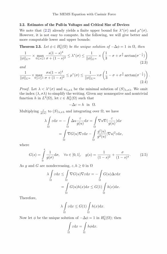
2.2. Estimates of the Pull-in Voltages and Critical Size of Devices

We note that (2.2) already yields a finite upper bound for λ∗(σ) and μ∗(σ).However, it is not easy to compute. In the following, we will give better andmore computable lower and upper bounds:

Theorem 2.3. Let φ ∈ H10 (Ω) be the unique solution of −Δφ = 1 in Ω, then

1‖φ‖L∞

× max0≤s≤1

s(1 − s)4

σ + (1 − s)2≤ λ∗(σ) ≤ 1

‖φ‖L∞×(

13


2 ))

(2.3)and

1‖φ‖L∞

× max0≤s≤1

σs(1 − s)4

σ + (1 − s)2≤ μ∗(σ) ≤ 1

‖φ‖L∞×σ(

13


2 ))

.

(2.4)

Proof. Let λ < λ∗(σ) and uλ,σλ be the minimal solution of (S)λ,σλ. We omitthe index (λ, σλ) to simplify the writing. Given any nonnegative and nontrivialfunction h in L2(Ω), let ε ∈ H1

0 (Ω) such that

−Δε = h in Ω.

Multiplying εg(u) to (S)λ,σλ and integrating over Ω, we have

λ

∫

Ω

εdx = −∫

Ω

Δuε

g(u)dx =

∫

Ω

∇u∇(ε

g(u))dx

=∫

Ω

∇G(u)∇εdx−∫

Ω

g′(u)g2(u)

|∇u|2εdx,

where

G(s) =

s∫

0

1g(σ)

dσ, ∀s ∈ [0, 1], g(s) =1

(1 − s)2+

σ

(1 − s)4. (2.5)

As g and G are nondecreasing, ε, h ≥ 0 in Ω

λ

∫

Ω

εdx ≤∫

Ω

∇G(u)∇εdx = −∫

Ω

G(u)Δεdx

=∫

Ω

G(u)h(x)dx ≤ G(1)∫

Ω

h(x)dx.

Therefore,

λ

∫

Ω

εdx ≤ G(1)∫

Ω

h(x)dx.

Now let φ be the unique solution of −Δφ = 1 in H10 (Ω); then

∫

Ω

εdx =∫

Ω

hφdx.


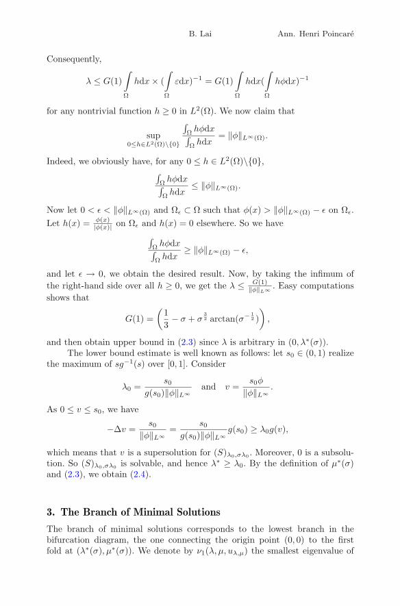
Consequently,

λ ≤ G(1)∫

Ω

hdx× (∫

Ω

εdx)−1 = G(1)∫

Ω

hdx(∫

Ω

hφdx)−1

for any nontrivial function h ≥ 0 in L2(Ω). We now claim that

sup0≤h∈L2(Ω)\{0}

∫

Ωhφdx

∫

Ωhdx

= ‖φ‖L∞(Ω).

Indeed, we obviously have, for any 0 ≤ h ∈ L2(Ω)\{0},∫

Ωhφdx

∫

Ωhdx

≤ ‖φ‖L∞(Ω).

Now let 0 < ε < ‖φ‖L∞(Ω) and Ωε ⊂ Ω such that φ(x) > ‖φ‖L∞(Ω) − ε on Ωε.Let h(x) = φ(x)

|φ(x)| on Ωε and h(x) = 0 elsewhere. So we have∫

Ωhφdx

∫

Ωhdx

≥ ‖φ‖L∞(Ω) − ε,

and let ε → 0, we obtain the desired result. Now, by taking the infimum ofthe right-hand side over all h ≥ 0, we get the λ ≤ G(1)

‖φ‖L∞ . Easy computationsshows that

G(1) =(

13


2 ))

,

and then obtain upper bound in (2.3) since λ is arbitrary in (0, λ∗(σ)).The lower bound estimate is well known as follows: let s0 ∈ (0, 1) realize

the maximum of sg−1(s) over [0, 1]. Consider

λ0 =s0

g(s0)‖φ‖L∞and v =

s0φ

‖φ‖L∞.

As 0 ≤ v ≤ s0, we have

−Δv =s0

‖φ‖L∞=

s0g(s0)‖φ‖L∞

g(s0) ≥ λ0g(v),

which means that v is a supersolution for (S)λ0,σλ0 . Moreover, 0 is a subsolu-tion. So (S)λ0,σλ0 is solvable, and hence λ∗ ≥ λ0. By the definition of μ∗(σ)and (2.3), we obtain (2.4).

3. The Branch of Minimal Solutions

The branch of minimal solutions corresponds to the lowest branch in thebifurcation diagram, the one connecting the origin point (0, 0) to the firstfold at (λ∗(σ), μ∗(σ)). We denote by ν1(λ, μ, uλ,μ) the smallest eigenvalue of


−Δ − 2λ(1−uλ,μ)3 − 4μ

(1−uλ,μ)5 , that is, the one corresponding to the followingDirichlet eigenvalue problem:

−Δϕ−(

2λ(1 − uλ,μ)3

+4μ

(1 − uλ,μ)5

)

ϕ = ν1(λ, μ, uλ,μ)ϕ, x ∈ Ω;

ϕ = 0, x ∈ ∂Ω.

In other words,

ν1(λ, μ, uλ,μ)

= infφ∈H1

0 (Ω)\{0}

∫

Ω

{|∇ϕ|2 − 2λ(1 − uλ,μ)−3ϕ2 − 4μ(1 − uλ,μ)−5ϕ2

}dx

∫

Ωϕ2dx

.

First, we give a Brezis–Vazquez type result, and refer the reader Brezis–Vazquez [10] or [[4], Lemma 4.1] for the proof of the following Lemma 3.1:

Lemma 3.1. Let f is C2 on [0, 1), positive, nondecreasing and convex such thatlimu→1−1 f(u) = ∞, and let Ω be a bounded domain in R

N . Suppose that u isa positive solution of

−Δu = λf(u), and 0 ≤ u < 1, x ∈ Ω;u = 0, x ∈ ∂Ω,

and consider any (classical) supersolution v of the above equation. If ν1(λ, u)> 0, then v ≥ u on Ω, and if ν1(λ, u) = 0, then v ≡ u on Ω.

Theorem 3.1. Now, consider the branch (λ, σλ) → uλ,σλ(x) of minimal solu-tions on (0, λ∗(σ)). Then the following hold:1. For each λ ∈ (0, λ∗(σ)), uλ,σλ(x) is a stable solution and λ → ν1(λ, σλ,uλ,σλ) is decreasing on (0, λ∗(σ)).

2. For each x ∈ Ω, the function λ → uλ,σλ(x) is differentiable and strictlyincreasing on (0, λ∗(σ)).

3. A semi-stable weak solution, called the extremal solution u∗(x) ∈ H10 (Ω)

exists for (S)λ∗,σλ∗ , indeed u∗(x) =: uλ∗,σλ∗(x) = limλ→λ∗ uλ,σλ(x) is welldefined semi-stable H1

0 (Ω)−weak solution of (S)λ∗,σλ∗ .4. No H1

0 (Ω)− weak solution exists for λ > λ∗(σ) and μ = σλ.

Proof. (1) Now we define

λ∗∗(σ) = sup{λ;uλ,σλ is a stable solution for (S)λ,σλ}.It is clear that λ∗∗ ≤ λ∗, and to show equality it suffices to prove that there isno minimal solution for (S)γ,σγ with γ > λ∗∗. For that, suppose ω is a minimalsolution of (S)λ∗∗+δ,σ(λ∗∗+δ) with δ > 0; then we would have, for λ ≤ λ∗∗(σ),

−Δω =λ∗∗ + δ

(1 − ω)2+σ(λ∗∗ + δ)(1 − ω)4

≥ λ

(1 − ω)2+

σλ

(1 − ω)4, x ∈ Ω.

Since for 0 < λ < λ∗∗(σ) the minimal solutions uλ,σλ are stable, it followsfrom Lemma 3.1 that 1 > ω ≥ uλ,σλ for all 0 < λ < λ∗∗(σ). Consequently,u = limλ↗λ∗∗ uλ,σλ exists in C2(Ω) and is a solution for (S)λ∗∗,σλ∗∗ . Now fromthe definition of λ∗∗(σ), we necessarily have ν1(λ∗∗, σλ∗∗, u) = 0; hence by


again applying Lemma 3.1, we obtain that u = ω and δ = 0 on Ω, which is acontradiction, and hence λ∗∗ = λ∗.

That λ → ν1(λ, σλ, uλ,σλ) is decreasing follows easily from the variationalcharacterization of ν1,λ,σλ, the monotonicity of λ → uλ,σλ, as well as themonotonicity of (1 − u)−3 + (1 − u)−5 with respect to u.

(2) Consider λ1 < λ2 < λ∗(σ), their corresponding minimal positivesolutions uλ1,σλ1 and uλ2,σλ2 , and let u be a positive solution for (S)λ2,σλ2 .For the monotone increasing series {un(λ1, σλ1;x)} defined in (2.1), we thenhave u > u1(λ1, σλ1;x) ≡ 0, and if un−1(λ1, σλ1;x) ≤ u in Ω, then{−Δ(u− un)=

[λ2

(1−u)2 + σλ2(1−u)4 )

]−[

λ1(1−un−1)2

+ σλ1(1−un−1)4

]≥ 0, x ∈ Ω

u− un = 0 x ∈ ∂Ω.

Then we, by maximum principle, have un(λ1, σλ1;x) ≤ u. Therefore,

uλ1,σλ1 = limn→∞un(λ1, σλ1;x) ≤ u

in Ω, and in particular uλ1,σλ1 ≤ uλ2,σλ2 in Ω. By the strong maximum prin-ciple, we have uλ1,σλ1 < uλ2,σλ2 in Ω.

Since each uλ,σλ are stable, then by setting

F (λ, uλ,σλ) := −Δuλ,σλ − λ

(1 − uλ,σλ)2− σλ

(1 − uλ,σλ)4,

we get that Fu(λ, uλ,σλ) is invertible for 0 < λ < λ∗(σ). It then follows fromthe Implicit Function Theorem that uλ,σλ is differentiable with respect to λ.

(3) Testing (S)λ,σλ on uλ,σλ ∈ H10 (Ω), we see that

∫

Ω

|∇uλ,σλ|2dx = λ

∫

Ω

(uλ,σλ

(1 − uλ,σλ)2+

σuλ,σλ

(1 − uλ,σλ)4

)

dx. (3.1)

Since by (1) uλ,σλ(x) is stable, we have

∫

Ω

|∇uλ,σλ|2dx ≥ λ

∫

Ω

(2u2

λ,σλ

(1 − uλ,σλ)3+

4σu2λ,σλ

(1 − uλ,σλ)5

)

dx.

And thus∫

u≥ 12

1(1 − uλ,σλ)5

≤ 4∫

u≥ 12

u2

(1 − uλ,σλ)5≤ C

∫

Ω

(1 − uλ,σλ)−4dx

≤ 12

∫

u≥ 12

1(1 − uλ,σλ)5

+ C,

by means of Young’s inequality, where the constant C is independent of λ.Since also

∫

u≤ 12

1(1−uλ,σλ)5 < C ′, for some C ′ > 0, we can deduce that for

every λ ∈ (0, λ∗(σ)),


∫

Ω

1(1 − uλ,σλ)5

< C,

for some C > 0 being independent of λ. By Holder’s inequality and (3.1), wehave

∫

Ω|∇uλ,σλ|2 < C for some C > 0. And so by the monotonicity lemma,

there exists a function u∗ := uλ∗,σλ∗ ∈ H10 (Ω) such that

∫

Ω

∇u∗∇ϕdx = λ

∫

Ω

(1

(1 − u∗)2+

σ

(1 − u∗)4

)

ϕdx for any ϕ ∈ H10 (Ω).

Moreover, by the monotonicity of the ν1(λ, σλ, uλ,σλ), we have ν1(λ∗, σλ∗, u∗)≥ 0, which means that u∗ is a semi-stable weak solution, even in the casewhere ‖u∗‖L∞ = 1.

(4) Let ω be a H10 (Ω)− weak solution of (S)λ,σλ, we first claim that for

any ψ ∈ C2([0, 1]) concave function so that ψ(0) = 0 we have that∫

Ω

∇ψ(ω)∇ϕ ≥ λ

∫

Ω

(1

(1 − ω)2+

σ

(1 − ω)4

)

ψ′(ω)ϕ (3.2)

for any ϕ ∈ H10 (Ω), ϕ ≥ 0. Indeed, by the concavity of ψ we get

∫

Ω

∇ψ(ω)∇ϕ =∫

Ω

ψ′(ω)∇ω∇ϕ =∫

Ω

∇ω∇(ψ′(ω)ϕ) −∫

Ω

ψ′′(ω)ϕ|∇ω|2

≥ λ

∫

Ω

(1

(1 − ω)2+

σ

(1 − ω)4

)

ψ′(ω)ϕ

for any ϕ ∈ C∞0 (Ω), ϕ ≥ 0, and by density we get (3.1) for any ϕ ∈ H1

0 (Ω),ϕ ≥ 0.

Inspired by [11], we define

h(ω) =

ω∫

0

dsg(s)

, h(ω) =

ω∫

0

ds(1 − ε)g(s)

,

for all 0 ≤ ω ≤ 1 and ε ∈ (0, 1). Where g(s) is defined in (2.5), i.e., g(s) =1

(1−s)2 + σ(1−s)4 . Now set Φ(ω) = h−1(h(ω)) for 0 ≤ ω ≤ 1. Obviously, we first

have Φ(0) = 0 and 0 < Φ(ω) < ω ≤ 1. By simple calculation, we also have

Φ′(ω) =(1 − ε)g(Φ(ω))

g(ω)< 1,

and

Φ′′(ω) =(1 − ε)[g(ω)g(Φ(ω))Φ′(ω) − g(Φ(ω))g′(ω)]

g2(ω)

=(1 − ε)g(Φ(ω))[(1 − ε)g′(Φ(ω)) − g′(ω)]

g2(ω)≤ 0.


And thus let ψ(ω) = Φ(ω), which satisfies∫

Ω

∇ψ(ω)∇ϕ ≥ (1 − ε)λ∫

Ω

g(ψ(ω))ϕ ∀ϕ ∈ H10 (Ω).

Hence, ψ(ω) is a H10 (Ω)-weak super-solution of (S)λ(1−ε),σλ(1−ε) so that 0 ≤

ψ(ω) < 1. Since 0 is a sub-solution for any λ > 0, we get the existence of aH1

0 (Ω)-weak solution vε of (S)λ(1−ε),σλ(1−ε) so that vε < 1. By standard ellipticregularity theory, vε is a classical solution. Since ε ∈ (0, 1) is arbitrary, we, bythe definition of λ∗(σ), get that there is no H1

0 (Ω) weak solution of (S)λ,μ forλ > λ∗(σ) and μ = σλ, which complete proof of (4).

4. Properties of the Extremal Solution on Υ(σ)

4.1. Regularity of the Extremal Solution

Lemma 4.1. Any weak solution u in H10 (Ω) of (S)λ,μ such that 1

1−u ∈ L52 N (Ω)

is a classical solution.

Proof. Suppose u is a weak solution such that 11−u ∈ L

52 N (Ω), which means

that 1(1−u)4 ∈ L

58 N (Ω). By Sobolev’s Theorem we can already deduce that

u ∈ C0,α(Ω) with α = 25 . To get more regularity, it suffices to show that u < 1

on Ω, but then if not, we consider x0 ∈ Ω such that u(x0) = ‖u‖C(Ω) = 1.Then, we have

|1 − u(x)| = |u(x0) − u(x)| ≤ C|x0 − x| 25 on Ω,

and then

+∞ >

∫

Ω

1(1 − u)

52 N

≥ C

∫

Ω

|x− x0|− 25 · 5

2 Ndx = +∞,

a contradiction, which implies that we must have u < 1.

Theorem 4.1. For any dimension 1 ≤ N ≤ 8, there exists a constant 0 ≤C(N,σ) < 1 independent of λ such that for any 0 < λ < λ∗ the minimalsolution uλ,μ satisfies ‖uλ,μ‖ < C(N,σ)

Consequently, u∗ = limλ→λ∗,σλ→σλ∗ uλ,σλ exists in the topology ofC2,α(Ω) with 0 < α < 1. It is the unique classical solution for (S)λ∗,σλ∗

and satisfies ν1(λ∗, σλ∗, u∗) = 0.

Proof. For simplicity, we denote uλ,μ by u. Since the minimal solutions arestable, we have

λ

∫

Ω

( 2(1 − u)3

+4σ

(1 − u)5)ω2dx <

∫

Ω

|∇ω|2dx for all 0 < λ < λ∗

and ω ∈ H10 (Ω). (4.1)

Now setting

ω = (1 − u)i − 1 > 0, where − 4 − 2√

5 < i < 0,


then (4.1) becomes

i2∫

Ω

(1 − u)2i−2|∇u|2dx > λ

⎛

⎝

∫

Ω

2[1 − (1 − u)i]2

(1 − u)3+∫

Ω

4σ[1 − (1 − u)i]2

(1 − u)5

⎞

⎠ .

(4.2)On the other hand, multiplying (Sλ,μ) by i2

1−2i [(1 − u)2i−1 − 1] and applyingintegration by parts yields that

i2∫

Ω

(1 − u)2i−2|∇u|2dx

= λi2

2i− 1

⎛

⎝

∫

Ω

{1 − (1 − u)2i−1

(1 − u)2+σ[1 − (1 − u)2i−1]

(1 − u)4

}

dx

⎞

⎠ . (4.3)

Hence (4.2) and (4.3) reduce to

σλ

[i2

2i− 1+ 4] ∫

Ω

1(1 − u)5−2i

dx

≤ λ

∫

Ω

{ i2

1 − 2i1

(1 − u)3−2i− i2

1 − 2i1

(1 − u)2− σi2

1 − 2i1

(1 − u)4

−2[1 − (1 − u)i]2

(1 − u)3− 4σ

(1 − u)5+

8σ(1 − u)5−i

}dx. (4.4)

From the choice of i we have i2

2i−1 + 4 > 0. So (4.3) and Holder’s inequalityimply that

∫

Ω

1(1 − u)5−2i

dx ≤ C

⎛

⎝

∫

Ω

dx(1 − u)3−2i

+∫

Ω

8σ(1 − u)5−i

dx

⎞

⎠

≤ C

⎛

⎝

∫

Ω

∣∣∣∣

1(1 − u)3−2i

∣∣∣∣

5−2i3−2i

⎞

⎠

3−2i5−2i

+

⎛

⎝

∫

Ω

∣∣∣∣

1(1 − u)5−i

∣∣∣∣

5−2i5−i

⎞

⎠

5−i5−2i

.(4.5)

Since 3−2i5−2i ,

5−i5−2i < 1, and then

∫

Ω1

(1−u)5−2i dx < C (−4 − 2√

5 < i < 0). From

Lemma 4.1, we have u∗ is a classical solution as long as 5N2 < 13+4

√5, which

happens when N ≤ 8. The uniqueness follows from Lemma 3.1.

4.2. Uniqueness of the Extremal Solution

We, from Theorem 4.1, first note that in the case N ≤ 9 the extremal solutionuλ∗,σλ∗ is the unique classical solution of equation (S)λ∗,σλ∗ for any σ > 0. Inthe following, we consider only the case that uλ∗,σλ∗ is a weak solution (i.e.,uλ∗,σλ∗ ∈ H1

0 (Ω)). Inspired by the ideas of [4,10–12], we establish the followinguseful characterization of the extremal solutions.

Theorem 4.2. For λ > 0, consider uλ,σλ ∈ H10 (Ω) to be a weak solution of

(S)λ,σλ such that ‖uλ,σλ‖L∞ = 1. Then the following assertions are equivalent:


1. ν1(λ, σλ, uλ,σλ) ≥ 0; that is, u satisfies∫

Ω|∇ϕ|2 ≥ ∫

Ω

(2λ

(1−uλ,σλ)3

+ 4σλ(1−uλ,σλ)5

)ϕ2 for all ϕ ∈ H1

0 (Ω);

2. λ = λ∗ and u = uλ∗,σλ∗ .

Theorem 4.2 can be easily obtained from the following lemma:

Lemma 4.2. Let u1, u2 be two H10 (Ω)-weak solutions of (S)λ,μ so that ν1(λ,

μ, ui) ≥ 0 for i = 1, 2. Then u1 = u2 almost everywhere in Ω.

Proof. Set g1(s) = λ(1−s)2 + μ

(1−s)4 , then g′′1 (s) > 0 for 0 ≤ s < 1. Now for any

θ ∈ [0, 1] and ϕ ∈ H10 (Ω), ϕ ≥ 0, we, by the convexity of g1(s), have that

Iθ,ϕ :=∫

Ω

∇(θu1 + (1 − θ)u2)∇ϕdx−∫

Ω

g1(θu1 + (1 − θ)u2)ϕdx

=∫

Ω

(θg1(u1) + (1 − θ)g1(u2) − g1(θu1 + (1 − θ)u2))ϕdx ≥ 0.

Since I0,ϕ = I1,ϕ = 0, the derivative of Iθ,ϕ at θ = 0, 1 provides∫

Ω

∇(u1 − u2)∇ϕ−∫

Ω

g′1(u2)(u1 − u2)ϕ ≥ 0,

∫

Ω

∇(u1 − u2)∇ϕ−∫

Ω

g′1(u1)(u1 − u2)ϕ ≤ 0,

for any ϕ ∈ H10 (Ω), ϕ ≥ 0. Testing the first inequality on ϕ = −(u1 − u2)−

and the second one on (u1 − u2)+, we get that∫

Ω

|∇(u1 − u2)−|2 −∫

Ω

g′1(u2)((u1 − u2)−)2dx ≤ 0

∫

Ω

|∇(u1 − u2)+|2 −∫

Ω

g′1(u1)((u1 − u2)+)2dx ≤ 0.

Since ν1(λ, μ, u1) ≥ 0, we have(1) either ν1(λ, μ, u1) > 0 and then u1 ≤ u2 a.e.,(2) or ν1(λ, μ, u1) = 0, which gives

∫

Ω

∇(u1 − u2)∇ϕ−∫

Ω

g′1(u1)(u1 − u2)ϕ = 0,

where ϕ = (u1 − u2)+. Since Iθ,ϕ ≥ 0 for any θ ∈ [0, 1] and I1,ϕ = ∂θI1,ϕ = 0,we get that

∂2θθI1,ϕ = −

∫

Ω

g′1(u1)((u1 − u2)+)3 ≥ 0,

we clearly have (u1 − u2)+ = 0 a.e., in Ω. Hence, u1 ≤ u2 a.e., in Ω. The sameargument applies to prove the reversed inequality, and the proof is complete.


Acknowledgements

The author thanks prof. Y. S., Yang for providing some valuable suggestionsand corresponding references. He also would like to express his sincere grati-tude to the referee for his careful review of the article. The research is supportedby NSFC (11201119, 11126155).

References

[1] Castorina, D., Esposito, P., Sciunzi, B.: Degenerate elliptic equations with sin-gular nonlinearities. Calc. Var. 34, 279–306 (2009)

[2] Flores, G., Mercado, G.A., Pelesko, J.A.: Dynamics and touchdown in electro-static MEMS. In: Proceeding of the 2003 International Conference on MEMS,Nano, and Smart Systems (ICMENS 2003) Banff, AB, 2003, IEEE ComputerSociety Press, Piscataway, 182–187

[3] Esposito, P., Ghoussoub, N., Guo, Y.: Mathematical analysis of partial differen-tial equations modeling electrostatic MEMS. Courant Lecture Notes in Mathe-matics, American Mathematical Society, vol. 20 (2010)

[4] Ghoussoub, N., Guo, Y.: On the partial differential equations of electrostaticMems devices: stationary case. Siam J. Appl. Math. 38, 1423–1449 (2007)

[5] Guo, Y., Pan, Z., Ward, M.J.: Touchdown and pull-in voltage behavior ofa MEMS device with varying dielectric properties. Siam J. Appl. Math. 66,309–338 (2005)

[6] Lin, F., Yang, Y.: Nonlinear non-local elliptic equation modelling electrostaticactuation. Proc. R. Soc. Lond., Ser. A Math. Phys. Eng. Sci. 463, 1323–1337(2007)

[7] Batra, R.C., Porfiri, M., Spinello, D.: Effects of casimir force on pull-in instabilityin micromembrances. Lett. J. Explor. Front. Phys. 77, 20010 (2007)

[8] Lamoreaux, S.K.: The Casimir force: background, experiments, and applica-tions. Rep. Progr. Phys. 68, 201–236 (2005)

[9] Mignot, F., Puel, J.P.: Sur une classe de problems non lineaires avec non linearitepositve, croissante, convex. Commun. Part. Differ. Equ. 8, 791–836 (1980)

[10] Brezis, H., Vazquez, J.L.: Blow-up solutions of some nonlinear elliptic problems.Rev. Mat. Univ. Complut. Madrid 10, 443–469 (1997)

[11] Brezis, H., Cazenave, T., Martel, Y., Ramiandrisoa, A.: Blow-up for ut − Δu =g(u) revisited. Adv. Part. Differ. Equ. 1, 73–90 (1996)

[12] Martel, Y.: Uniqueness of weak extremal solutions of nonlinear elliptic problems.Houst. J. Math. 23, 161–168 (1997)

Baishun LaiInstitute of Contemporary MathematicsHenan UniversityKaifeng 475004People’s Republic of Chinae-mail: [email protected]

Communicated by Nader Masmoudi.

Received: June 11, 2013.

Accepted: January 30, 2014.

on the partial differential equations of electrostatic mems devices with effects of casimir force

Documents