on the optimality of answer-copying indices: theory and...

On the optimality of answer-copying indices:

theory and practice∗

Mauricio Romero†‡

Alvaro Riascos §‡

Diego Jara‡

May 13, 2015

Abstract

Multiple-choice exams are frequently used as an efficient and objectivemethod to assess learning, but they are more vulnerable to answer copyingthan tests based on open questions. Several statistical tests (known asindices in the literature) have been proposed to detect cheating; however,to the best of our knowledge they all lack mathematical support thatguarantees optimality in any sense. We partially fill this void by derivingthe uniformly most powerful (UMP) test under the assumption that theresponse distribution is known. In practice, however, we must estimate abehavioral model that yields a response distribution for each question. Asan application, we calculate the empirical type I and type II error rates forseveral indices that assume different behavioral models using simulationsbased on real data from twelve nationwide multiple-choice exams taken by5th and 9th graders in Colombia. We find that the most powerful indexamong those studied, subject to the restriction of preserving the type Ierror, is one based on the work of Wollack (1997) and van der Linden andSotaridona (2006) and is superior to the indices studied and developed byWesolowsky (2000) and Frary, Tideman, and Watts (1977).

Keywords: ω Index , answer copying, false discovery rate, Neyman-PearsonLemma.∗Corresponding author: Mauricio Romero. E-mail: [email protected]. The authors

would like to thank the ICFES for financial support during the early stages of this project;the editor, Dan McCaffrey; two anonymous reviewers; Nicola Persico; Decio Coviello; andJulian Marino and his group of statisticians for their valuable comments and suggestions onprevious versions of the manuscript.†University of California - San Diego.‡Quantil | Matematicas Aplicadas§Universidad de los Andes and Quantil | Matematicas Aplicadas.

1

mailto:[email protected]

1 Introduction

Multiple-choice exams are frequently used, as they are considered by many tobe an efficient and objective way of evaluating knowledge. Nevertheless, theyare more vulnerable to answer copying than tests based on open questions.Answer-copy indices provide a statistical tool for detecting cheating by examin-ing suspiciously similar response patterns between two students. However, theseindices have three problems. First, similar answer patterns between a pair ofstudents may occur without answer copying. For example, two individuals withvery similar educational backgrounds are likely to provide similar answers. Thesecond problem is that a statistical test (an index) is by no means a conclusivebasis for accusing someone of copying, since it is impossible to completely elim-inate type I errors. In other words, it is possible that two individuals may sharethe same response pattern by chance. Finally, every index assumes responsesare stochastic. If the assumed probability distribution is incorrect, the indexcan lead to incorrect conclusions. Furthermore, all the indices in the literatureare ad hoc and there are no theoretical results that support the use of one indexover the other.

Wollack (2003) compares several indices using real data and finds that amongthose that preserve size (i.e., indices that have an empirical type I error ratebelow the theoretical one. That is, in practice they are less than or equallylikely to erroneously reject the null hypothesis than suggested by the size of thetest) the ω index (based on the work of Wollack (1997)) is the most powerfulone. However, the set of indices studied is not comprehensive and in particulardoes not include the index developed by Wesolowsky (2000).

Thus there are two gaps in the literature that this article seeks to fill. First,it provides theoretical foundations for validating the use of indices that rejectthe null hypothesis of no cheating for a large number of identical answers underthe assumption that student responses are stochastic.

Second, we calculate the empirical type I and type II error rates of tworefinements of the indices first developed by Frary et al. (1977), the ω and γindices based on the work of Wollack (1997) and Wesolowsky (2000) respectively.Using Monte Carlo simulations and data from the SABER tests taken by 5thand 9th graders in Colombia in May and October of 2009 we find that theconditional version of the standardized index first developed by Wollack (1997)is the most powerful among those that preserve size.

The article is organized as follows. The second section derives an opti-mal statistical test (index) to detect answer copying using the Neyman-Pearsonlemma. The third section presents two of the most widely used indices, whichare based on the work of Wollack (1997), Frary et al. (1977), Wesolowsky (2000),and van der Linden and Sotaridona (2006). The fourth section presents a briefsummary of the data used and is followed by a section that presents the method-ology of the Monte Carlo simulations used to find the empirical type I and typeII error rates (to test which behavioral model gives the best results) and itsresults. Finally, the sixth section concludes.

2

2 Applying the Neyman-Pearson lemma to an-swer copying

It is normal for two answer patterns to have similarities by chance. Answer-copying indices are used to detect similarities that are so unlikely to happennaturally that answer copying becomes a more natural explanation than chance.Most answer-copy indices are calculated by counting the number of identicalanswers between the test taker suspected of copying and the test taker suspectedof providing answers. For examples see van der Linden and Sotaridona (2004,2006); Sotaridona and Meijer (2003, 2002); Sotaridona, van der Linden, andMeijer (2006); Holland (1996); Frary et al. (1977); Cohen (1960); Bellezza andBellezza (1989); Angoff (1974); Wesolowsky (2000); Wollack (1997). In all theseindices the null hypothesis is the same: There is no cheating.

All these indices are ad hoc since they are not derived to be optimal inany sense. To the authors’ knowledge, this article presents the first effort torationalize the use of these indices to detect answer copying using the Neyman-Pearson lemma (NPL) (Neyman & Pearson, 1933) resulting in the uniformlymost powerful (UMP) test (index), assuming we know the underlying probabilitythat two individuals have the same answer in each question. However, we mustturn to empirical data to find the performance of each index since differentbehavioral models result in different response probability distributions.

First, we state the problem formally. Let us assume that there are N ques-tions and n alternatives for each question. We are interested in testing whetherthe individual who cheated (denoted by c) copied from the individual who sup-posedly provided the answers (denoted by s). Let γcs be the number of questionsthat c copied from s. The objective is to test the following hypotheses:

H0 : γcs = 0

H1 : γcs > 0

Let Icsi be equal to one when individuals c and s have the same answer toquestion i and zero otherwise. Then, the number of common answers betweenc and s can be expressed as:

Mcs =

N∑i=1

Icsi. (1)

Under the null hypothesisMcs is the sum ofN independent Bernoulli randomvariables, each with a different probability of success πi, equal to the probabilitythat individual c has the same answer as individual s in question i. The distri-bution of Mcs is known as a Poisson binomial distribution. Let B(π1, ..., πN ) bethat distribution and fN (x;π1, ..., πN ) be the probability mass function (pmf)

at x. Note that fN (x;π1, ..., πN ) =∑A∈Fx

(∏i∈A πi

) (∏j∈Ac(1− πj)

), where

Fx = {A : A ⊂ {1, ..., N}, |A| = x}. If π1 = π2 = ... = πN = π then the Poisson

3

binomial distribution reduces to a standard binomial distribution. Althoughcomputing fN can be computationally intensive, efficient algorithms have beenderived by Hong (2013).

Now, let A denote the set of questions that student c copied from s. Then if|A| = k, it means that γcs = k, and Mcs has the pmf fN (x;π1, ..., πN , A), where

we define fN (x;π1, ..., πN , A).= fN (x;π′1, .., π

′N ) such that

π′i =

{1 if i ∈ Aπi if i 6∈ A

For example, say that there are 50 questions and that the students copiedquestions 1, 10 and 50 (i.e., A = {1, 10, 50}) then

fN (x;π1, ..., πN , A) = fN (x; 1, π2, ..., π9, 1, π11, ..., π49, 1).

Before we continue let us state the Neyman-Pearson lemma::

Theorem 1. Neyman-Pearson lemma (Casella & Berger, 2002)Consider testing H0 : θ = θ0 against H1 : θ = θ1 where the pmf is f(x|θi),

i = 0, 1, using a statistical test (index) with rejection region R (and thereforeits complement, Rc, is the non-rejection region) that satisfies

x ∈ R if f(x|θ1) > f(x|θ0)δ

x ∈ Rc if f(x|θ1) < f(x|θ0)δ(2)

for some δ ≥ 0, and

α = PH0(X ∈ R) (3)

where PHi(X ∈ A) := P (X ∈ A) if θ = θi. Then

1. (Sufficiency) Any test (index) that satisfies equations 2 and 3 is a UMPlevel α test (index).

2. (Necessity) If there exists a test (index) satisfying equations 2 and 3 withδ > 0, then every UMP level α test (index) is a size α test (index) -satisfying 3 - and every UMP level α test (index) satisfies 2 except perhapson a set A such that PH0

(X ∈ A) = PH1(X ∈ A) = 0.

Notice that NPL implies that a likelihood ratio test is the uniformly mostpowerful test for simple hypothesis testing. Let us apply the NPL to the simplehypothesis test H0 : A = A0 and H1 : A = A1, where A0 = ∅ (i.e., there is nocheating) and A1 is a set of questions. If in the data we observe x questionsanswered equally by individuals c and s then the likelihood ratio test would be:

λA(x) =fN (x;π1, ..., πN , A1)

fN (x;π1, ..., πN , A0)=fN (x;π1, ..., πN , A1)

fN (x;π1, ..., πN )

4

Now we must find the critical value of the test. In other words, we need thegreatest value c such that under the null we have:

1− PH0

(fN (x;π1, ..., πN , A)

f(x;π1, ..., πN )< c

)= PH0

(fN (x;π1, ..., πN , A)

fN (x;π1, ..., πN )> c

)≤ α

For any given pair of simple hypotheses (H0 : A = A0 , H1 : A = A1) weknow how to find the UMP (by using the NPL) test. The following lemma willallow us to find the UMP test for more complex alternative hypothesis (e.g.,H1 : {A : |A| ≥ 1}) as it lets us exploit the fact that distribution families withthe monotone likelihood ratio property have a UMP that does not depend onthe alternative hypothesis (see Section 3.4 in Lehmann and Romano (2005)).

Lemma 1. λA(x) = fN (x;π1,...,πN ,A)fN (x;π1,...,πN ) is increasing in x ∈ {0, ..., N} for all A.

Before we present the proof we must first recall some useful results provedby Wang (1993).

Theorem 2 (Theorem 2 in Wang (1993)). The pmf of a Poisson binomialsatisfies the following inequality:

fN (x;π1, π2, ..., πN )2 > C(x)fN (x+ 1;π1, π2, ..., πN )fN (x− 1;π1, π2, ..., πN )

where C(x) = max(x+1x , N−x+1

N−x

)which has as an immediate corollary:

Corollary 1. The pmf of a Poisson binomial satisfies the following inequality:

fN (x;π1, π2, ..., πN )2 > fN (x+ 1;π1, π2, ..., πN )fN (x− 1;π1, π2, ..., πN )

Now we are ready to prove the lemma:

Proof of Lemma 1. The proof will be done by induction on the size of A.Base Case:First, consider the case |A| = 1. Without loss of generality, as the pmf

is invariant to permutations of the πi’s (Wang, 1993), assume A = {1}. Thenumerator in the lemma’s quotient is 0 for x = 0, so we proceed to provemonotonicity λA(x) in x for x ≥ 1. Likewise, the case N = 1 follows trivially,so we assume N > 1.

For simplicity, we call g(x) = fN−1(x;π2, . . . , πN ). First, note that

fN (x;π1, . . . , πN ;A) = g(x− 1).

Second, corollary 1 states that g(x − 1)g(x + 1) < g(x)2. Third, we can writefN (x;π1, π2, . . . , πN ) = π1g(x− 1) + (1− π1)g(x). With these observations we

5

have

fN (x;π1, . . . , πN ;A)

fN (x;π1, . . . , πN )=

g(x− 1)

π1g(x− 1) + (1− π1)g(x)× π1g(x) + (1− π1)g(x+ 1)

π1g(x) + (1− π1)g(x+ 1)

<π1g(x)g(x− 1) + (1− π1)g(x)2

[π1g(x− 1) + (1− π1)g(x)][π1g(x) + (1− π1)g(x+ 1)]

=g(x)

π1g(x) + (1− π1)g(x+ 1)

=fN (x+ 1;π1, . . . , πN ;A)

fN (x+ 1;π1, . . . , πN ).

Inductive Step:

Suppose λA(x) = fN (x;π1,...,πN ,A)fN (x;π1,...,πN ) is increasing in x ∈ {0, ..., N} for all A,

such that |A| = k. Without loss of generality, consider a set A such that 1 6∈ Aand |A| = k. Let A = A ∪ {1} (so |A| = k + 1). Then,

λA(x) =fN (x;π1, ..., πN , A)

fN (x;π1, ..., πN )

=fN (x; 1, .., πN , A)

fN (x;π1, ..., πN )

=fN (x; 1, .., πN , A)

fN (x; 1, ..., πN )× fN (x; 1, ..., πN )

fN (x;π1, ..., πN )

=fN (x; 1, .., πN , A)

fN (x; 1, ..., πN )× fN (x;π1, ..., πN , {1})

fN (x;π1, ..., πN )

<fN (x+ 1; 1, .., πN , A)

fN (x+ 1; 1, ..., πN )× fN (x+ 1;π1, ..., πN , {1})

fN (x+ 1;π1, ..., πN )

=fN (x+ 1;π1, .., πN , A)

fN (x+ 1;π1, ..., πN )

= λA(x+ 1)

Given that fN (x;π1,...,πN ;A)fN (x;π1,...,πN ) is increasing in x for all A then we have that for

every c there exists a k∗ such that PH0

(fN (x;π1,...,πN ,A)fN (x;π1,...,πN ) < c

)=∑k∗

w=0 fN (w;π1, ..., πN ).

The last equality also comes from the fact that PH0

(fN (x;π1,...,πN ;A)fN (x;π1,...,πN ) = a

)=

PH0 (Mcs = b) = fN (b;π1, ..., πN ), where b is such that fN (b;π1,...,πN ;A)fN (b;π1,...,πN ) = a.

Notice that b is unique due to the strict monotonicity of fN (x;π1,...,πN ;A)fN (x;π1,...,πN ) .

In particular for a given size α of the test we can find k∗ such that

1− PH0

(fN (x;π1, ..., πN , A)

f(x;π1, ..., πN )< c

)= 1−

k∗∑w=0

f(w;π1, ..., πN ) ≤ α

6

Then, if we reject the null hypothesis when Mcs > k∗, we get the UMP fora particular set A. However, the rejection region is the same for all A. Thus, ifwe reject the null hypothesis when Mcs > k∗, we get the UMP for all A suchthat |A| ≥ 1.

The previous derivation is the first, to the best of our knowledge, that guar-antees optimality of indices that reject the null hypothesis for large values ofMcs. In other words we have derived the most powerful index among thosewith size α and shown that this index is one that rejects the null hypothesisfor large values of Mcs. As many existing indices count the number of matchesand compare them to a critical value, this implies that they have the same func-tional form as the UMP. Indices that reject the null hypothesis for large valuesof identical incorrect answers (such as the K-index (Holland, 1996)) can only beUMP if we assume that correct answers are never the result of answer copying.

However, an underlying assumption we have used so far is that we observethe value of πi for all i. Instead, we observe the actual answers that individualsprovided to the questions in the exam and must infer the value of πi for all ifrom these observations. Therefore, we cannot actually achieve the UMP. Thecloser we are to correctly estimating the πi’s, the closer our index will be to theUMP.

Additionally, our theoretical result does not cover all possible answer-copyingindices. For example, in this article we only consider blind copying events andnot shift-copy events in which c copies answers to the next or previous (insteadof current) question by mistake. Notice that in the presence of shift-copy eventsthe number of common answers between c and s might be smaller than γcs.Additionally, Belov (2011) showed that in the presence of variable sections (testsoften have an “operational” section with identical questions for all students anda “variable” section with different questions for adjacent students) the model ofPoisson trials does not work because each πi becomes a discrete random variable.Belov (2011) develops an index (the VM-index) that considers shift-copy eventsand takes into account the presence of variable sections. Because of its natureour theoretical results do not speak to the optimality of the VM-index.

In a seminal article Frary et al. (1977) developed the first indices, known asg1 and g2, that reject the null hypothesis for large values of Mcs. Wollack (1997),van der Linden and Sotaridona (2006) and Wesolowsky (2000) have proposedfurther refinements of the methods of Frary et al. (1977) methods. The maindifference between these indices is how they estimate the πi’s. The next sectionoutlines a methodology to compare indices, in terms of their type I and type IIerror rate, using real data from multiple-choice exams. We present the resultof comparing the two widely used indices developed by Wesolowsky (2000) andWollack (1997), as they have never been compared in the literature before andthey both reject the null hypothesis for large values of Mcs (and therefore theiruse is justified by the results from this section).

7

3 Copy Indices

Let us assume that student j has a probability πjiv of answering option v onquestion i. The probability that two students have the same answer on questioni (πi) can be calculated in two ways. First, assuming independent answers, theprobability of obtaining the same answer is πi =

∑nv=1 π

civπ

siv.

Second, we could think of the answers of individual s as being fixed, as ifhe were the source of the answers and c the student who copies. In the absenceof cheating, conditional on the answers of s, the probability that individual chas the same answer as individual s in question i is πi = πcivs , where πcivs isthe probability that individual c answered option vs which was chosen by s inquestion i.

A discussion of these two approaches is given in Frary et al. (1977) andvan der Linden and Sotaridona (2006). The first is known as the unconditionalindex and is symmetric in the sense that the choice of who is s and who is cis irrelevant since πi is the same either way. The second is known as the con-ditional index and it is not symmetric, opening the possibility that the indexrejects the null hypothesis that student a copied from student b but not rejectingthe null hypothesis that b copied from a. The details of each situation deter-mine which approach is appropriate. If we believe students copied from eachother or answered the test jointly then a conditional index is undesirable, butif we believe that a student is the source (for whatever reason) of answers butdid not collaborate with the cheater, then a conditional index might be moreappropriate. We study both conditional and unconditional indices.

Indices vary along three dimensions. The first dimension is how they esti-mate πjiv. The second is whether they are a conditional or an unconditionalindex. Finally, they vary in how critical values are calculated. They either usethe exact distribution (a Poisson binomial distribution) or a normal distribution,by applying some version of the central limit theorem. This is common prac-tice as computing the pmf of a Poisson binomial is an NP-hard problem whichcan be computationally intensive and often requires summing a large numberof small quantities, which can lead to numerical errors.

In order to use the central limit theorem in this context, recall Mcs is the sumof N Bernoulli variables and has mean

∑Ni=1 πi and variance

∑Ni=1 πi(1 − πi).

ThusMcs−

∑Ni=1 πi√∑N

i=1 πi(1−πi)converges in distribution to a standard normal distribution

as N goes to infinity, as long as πi ∈ (0, 1) for all i. In practice this means thereis no question with an option that no student will choose (see section 2.7 ofLehmann (1999) for more details). There are two advantages to the normalapproximation. First, critical values are easier to calculate and more precise(computationally) and second, it allows for a finer choice of critical values.

As mentioned before, Frary et al. (1977) developed the first indices thatreject the null hypothesis for large values of Mcs. However, both Wesolowsky(2000) and Wollack (2003) show that variations of the original method proposedby Frary et al. (1977) yield superior results, and in this article we study theindices they developed. The first variation is the ω index developed by Wollack

8

(1997) that assumes there is an underlying nominal response model. The secondvariation is the γ index developed by Wesolowsky (2000).

3.1 ω index

The ω index (Wollack, 1997) assumes a nominal response model that allows theprobability of answering a given option to vary across questions and individuals.As before, let N be the number of questions and n the number of alternativesfor answering each question. Suppose that an individual with skill θj , who doesnot copy, has a probability πiv of choosing option v in response to question i.In other words:

πjiv ≡ πiv(θj) =eξiv+λivθj∑nh=1 e

ξih+λihθj, (4)

where ξiv y λiv are model parameters and are known as the intercept and slope,respectively. The intercept and slope can vary across questions. The parametersof the questions (ξiv and λiv) are estimated using marginal maximum likelihood,while ability is estimated using the Expected A Posteriori (EAP) method. Theestimation is performed using the rirt package in R (Germain, Abdous, & Valois,2014). The ability is estimated taking into account that a correct answer to a“difficult” question indicates a higher ability than a correct answer to a “simple”question. More information on marginal maximum likelihood and EAP can befound in van der Linden and Hambleton (1997) and Hambleton, Swaminathan,and Rogers (1991).

Let ω1 and ω2 be the unconditional and conditional (exact) versions of thisindex (following somewhat the g1 and g2 notation of Frary et al. (1977)) and letωs1 and ωs2 be the standardized versions (i.e., they use the normal distributionto find the critical values of the index). Specifically,

ω1 = Mcs ∼ B(π1, ..., πN )

ω2 = Mcs ∼ B(π′1, ..., π′N )

ωs1 =Mcs−

∑Ni=1 πi√∑N

i=1 πi(1−πi)∼ N (0, 1)

ωs2 =Mcs−

∑Ni=1 π

′i√∑N

i=1 π′i(1−π′i)

∼ N (0, 1) ,

where πi =∑nv=1 π

civπ

siv and πjiv is calculated using equation 4. Similarly,

π′i = πcivs = eξivs+λivsθc∑n

h=1 eξih+λihθc

, where vs is the answer of individual s to question i.

3.2 γ index

The indices developed by Wesolowsky (2000) assume that the probability thatstudent j has the correct answer (option v) in question i is given by:

πjiv = (1− (1− ri)aj )1/aj , (5)

9

where ri is the proportion of students that had the right answer to question i.The parameter aj is estimated by solving the equation∑N

i=1 πjiv

N= cj ,

where cj is the proportion of questions answered correctly by individual j. Fi-nally, we need the probability that student j chooses option v among those thatare incorrect, which is estimated as the proportion of students with an incorrectanswer that chose each incorrect option. Thus, we have an estimate πjiv forevery individual j, every question i and every option v. Let us denote by γ1and γ2 the unconditional and conditional version of this index and by γs1 andγs2 their standardized version, respectively. Specifically,

γ1 = Mcs ∼ B(π1, ..., πN )

γ2 = Mcs ∼ B(π′1, ..., π′N )

γs1 =Mcs−

∑Ni=1 πi√∑N

i=1 πi(1−πi)∼ N (0, 1)

γs2 =Mcs−

∑Ni=1 π

′i√∑N

i=1 π′i(1−π′i)

∼ N (0, 1) ,

where πi =∑nv=1 π

civπ

siv and πjiv is calculated using equation 5 if v is the correct

answer and if not, as the proportion of students with answer v among those thatchose any incorrect option. Finally, π′i = πcivs = (1− (1− ri)ac)1/ac if individuals chose the correct option; if individual s chose an incorrect answer then π′i isequal to the proportion of students with answer vs among those that chose anyincorrect option.

Before we compare how the different versions of the ω and the γ index farein practice, the following section presents the data used.

4 Data

In Colombia, all students enrolled in 5th, 9th and 11th grades, whether attend-ing a private or public school, are required to take a standardized, multiple-choice test known as SABER. These exams are intended to measure the perfor-mance of students and schools across several areas. The Instituto Colombianopara la Evaluacion de la Educacion (ICFES), a government institution, is incharge of developing, distributing and applying these exams. Scores on the testtaken in 11th grade are used by most universities in Colombia as an admissioncriterion, but there are no consequences for 5th and 9th graders based on theirtest performance. The ICFES also evaluates all university students during theirsenior year. In this article, we analyze all the 5th and 9th grade tests for 2009.Each grade (5th and 9th) takes three tests: science, mathematics and language.Students at schools whose academic year ends in December (both private and

10

public) take the exam in September, while students at schools whose academicyear ends in June (mainly private schools) take the exam in May. In total thereare two dates, two grades and three subjects, for a total of 12 exams. The fol-lowing codes are assigned by the ICFES to each exam: per grade, 5 for 5th and9 for 9th. Per area, 041 for mathematics, 042 for language and 043 for science.Per date, F1 for May and F2 for October. For example, exam 9041F2 is takenby 9th graders for mathematics in October. A brief overview of each test ispresented in Table 1.

The database contains the answers chosen by each individual to every ques-tion on all of the tests, as well as the examination room where the exam wastaken. The correct answers for each exam are also available.

Table 1: Summary statistics

Test Subject Grade Month Questions Students Examination Rooms5041F1 Math 5th May 48 60,099 3,4215041F2 Math 5th Oct 48 403,624 31,8275042F1 Language 5th May 36 60,455 3,4415042F2 Language 5th Oct 36 402,508 31,6425043F1 Science 5th May 48 60,404 3,4325043F2 Science 5th Oct 48 405,537 31,8339041F1 Math 9th May 54 44,577 1,1109041F2 Math 9th Oct 54 303,233 9,0599042F1 Language 9th May 54 44,876 1,1109042F2 Language 9th Oct 54 302,781 9,0449043F1 Science 9th May 54 44,820 1,1079043F2 Science 9th Oct 54 30,3723 9,053Source: ICFES. Calculations: Authors.

5 Index Comparison

In this section we compare the different versions of the ω and the γ indices.In order to do this we evaluate the type I and type II error rates by creatingsynthetic samples in which we control the level of cheating between individuals.

5.1 Methodology

To find the empirical type I error rate, individuals who could not have possiblycopied from one another are paired together and tested for cheating using a par-ticular index. This is done by pairing individuals who took the exam in differentrooms, thus eliminating the possibility of answer copying to some extent. Wecannot rule out the possibility that proctors give out the answers to students,

11

but as these are low-stakes exams for teachers and schools we do not believe thisis a first-order concern. Additionally, as the exam takes place at the same dateand time nationwide, we do not believe that students are able to share theiranswers with students in other examination rooms.

The empirical type I error rate is calculated as the proportion of pairs forwhich the index rejects the null hypothesis. To find the empirical type II errorrate, we take these answer-copy free pairs and simulate copying by forcing spe-cific answers to be the same. The proportion of pairs for which the index rejectsthe null hypothesis is the power of the index (recall that the power of the test isthe complement of the type II error rate, i.e., Power = 100%−Type II Error).

To make things clearer, let c denote the test taker suspected of cheating, sthe test taker believed to have served as the source of answers. The steps takento find the type I error rate and the power of each index are as follows:

1. 100,000 pairs are chosen in such a way that for each couple the individ-uals performed the exam in different examination rooms. Each pair isconstructed by randomly selecting two examination rooms, and then ran-domly selecting one student from each examination room. Then withineach pair the students are randomly ordered.The first student is labeleds (the source) and the second student is labeled c (the copier). This dis-tinction is only important for the conditional (subscript 2) version of theindices. The selection process is done with replacement.

2. The answer-copy methodology is applied to these pairs, and the proportionof pairs for which the index rejects the null hypothesis is the empirical typeI error rate estimator.

3. To calculate the power of the index, the answer pattern for individual c ischanged by replacing k of his answer to match those of individual s. Forexample, let us assume the answer pattern for s is ACBCDADCDAB,which means that there were 11 questions and that he/she answered A tothe first question, C to the second question, and so on. Also assume thatthe original answer pattern of c without copying is DCABCDAABCB.Let k be 5 and let us assume that the randomly selected questions were1,4,5,10,11. This means that the modified (with copying) answer patternsfor c will be ACACDDAABAB. Specifically,

(a) The level of copying k (the number of answers transferred from s toc) is set.

(b) k questions are selected randomly.

(c) Individual c’s answers for the k questions are changed to replicatethose of individual s. Answers that were originally identical count aspart of the k questions being changed.

4. We apply the answer-copy methodology to the pairs whose exams havebeen altered. The proportion of pairs accused of cheating is the power ofthe index for a copying level of k.

12

5.2 Results

Throughout the analysis a size (α) value of 0.1% is used and the power of theindex is calculated at copying levels (k) of 1, 5, 10, 15, 20, ..., N , where N is thenumber of questions in the exam. To make the results as comparable as possibleand reduce the noise generated by using different random draws, the 100,000pairs are picked first and then the different indices are applied to the same setof randomly generated pairs.

5.2.1 Type I error rate

As can be seen in tables 2 and 3 the γ2, γs2 , and ω2 indices have an empiricaltype I error rate that is consistently above the theoretical type I error rate ofone in one thousand and is also statistically significant. The γ1 index (which isthe exact index developed by Wesolowsky (2000)) empirical error rate is abovethe theoretical one in several cases.

Based on these results, we discard the γ2, γs2 and ω2 indices and restrict thesearch for the most powerful index to γ1, γs1 , ω1, ωs1 and ωs2.

13

Table 2: Type I error for the γ indices

Exam Subject Grade Month γ1 γ2 γs1 γs25041F1 Math 5th May 0.67 2.81∗∗∗ 0.43 0.74

(0.08) (0.17) (0.07) (0.09)5041F2 Math 5th October 1.02 3.17∗∗∗ 0.71 1.1

(0.1) (0.18) (0.08) (0.1)5042F1 Language 5th May 1.01 2.09∗∗∗ 0.63 1.04

(0.1) (0.14) (0.08) (0.1)5042F2 Language 5th October 1.4∗∗∗ 2.33∗∗∗ 1.02 1.45∗∗∗

(0.12) (0.15) (0.1) (0.12)5043F1 Science 5th May 1.01 2.33∗∗∗ 0.71 1.2∗∗

(0.1) (0.15) (0.08) (0.11)5043F2 Science 5th October 0.9 2.07∗∗∗ 0.74 1.38∗∗∗

(0.09) (0.14) (0.09) (0.12)9041F1 Math 9th May 1.68∗∗∗ 2.38∗∗∗ 1.29∗∗∗ 1.3∗∗∗

(0.13) (0.15) (0.11) (0.11)9041F2 Math 9th October 2.55∗∗∗ 2.33∗∗∗ 1.93∗∗∗ 1.59∗∗∗

(0.16) (0.15) (0.14) (0.13)9042F1 Language 9th May 0.69 1.86∗∗∗ 0.4 0.95

(0.08) (0.14) (0.06) (0.1)9042F2 Language 9th October 0.89 1.97∗∗∗ 0.54 1.2∗∗

(0.09) (0.14) (0.07) (0.11)9043F1 Science 9th May 1.67∗∗∗ 2.25∗∗∗ 1.27∗∗∗ 1.57∗∗∗

(0.13) (0.15) (0.11) (0.13)9043F2 Science 9th October 1.41∗∗∗ 2.11∗∗∗ 1.16∗ 1.72∗∗∗

(0.12) (0.15) (0.11) (0.13)Number of innocent pairs accused of copying (for every 1,000 pairs) at α = 0.1%. Standarderrors in parentheses. For each exam-index combination we test whether the empirical type Ierror rate (α) is greater than the theoretical one α = 0.1% (i.e., H0 : α ≤ 0.1% vs H1 = α >0.1%). The asterisks denote the level at which the null hypothesis can be rejected. ∗ p < 0.10,∗∗ p < 0.05, ∗∗∗ p < 0.01. Source: ICFES. Calculations: Authors.

14

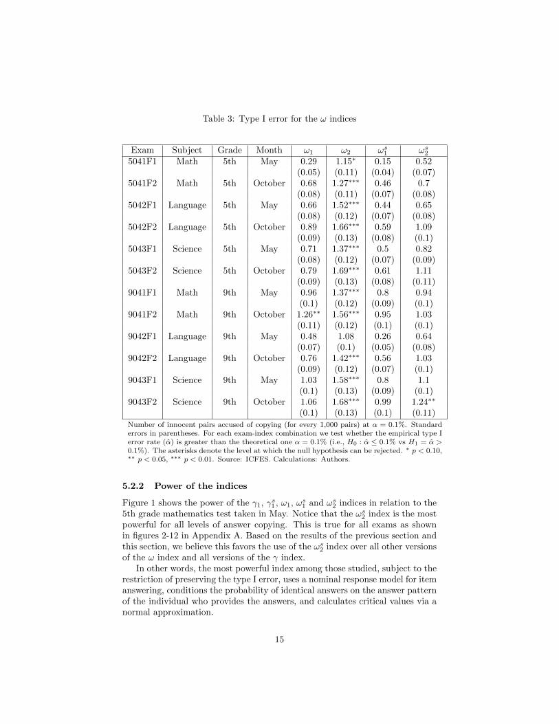
Table 3: Type I error for the ω indices

Exam Subject Grade Month ω1 ω2 ωs1 ωs25041F1 Math 5th May 0.29 1.15∗ 0.15 0.52

(0.05) (0.11) (0.04) (0.07)5041F2 Math 5th October 0.68 1.27∗∗∗ 0.46 0.7

(0.08) (0.11) (0.07) (0.08)5042F1 Language 5th May 0.66 1.52∗∗∗ 0.44 0.65

(0.08) (0.12) (0.07) (0.08)5042F2 Language 5th October 0.89 1.66∗∗∗ 0.59 1.09

(0.09) (0.13) (0.08) (0.1)5043F1 Science 5th May 0.71 1.37∗∗∗ 0.5 0.82

(0.08) (0.12) (0.07) (0.09)5043F2 Science 5th October 0.79 1.69∗∗∗ 0.61 1.11

(0.09) (0.13) (0.08) (0.11)9041F1 Math 9th May 0.96 1.37∗∗∗ 0.8 0.94

(0.1) (0.12) (0.09) (0.1)9041F2 Math 9th October 1.26∗∗ 1.56∗∗∗ 0.95 1.03

(0.11) (0.12) (0.1) (0.1)9042F1 Language 9th May 0.48 1.08 0.26 0.64


(0.09) (0.12) (0.07) (0.1)9043F1 Science 9th May 1.03 1.58∗∗∗ 0.8 1.1

(0.1) (0.13) (0.09) (0.1)9043F2 Science 9th October 1.06 1.68∗∗∗ 0.99 1.24∗∗


5.2.2 Power of the indices

Figure 1 shows the power of the γ1, γs1 , ω1, ωs1 and ωs2 indices in relation to the5th grade mathematics test taken in May. Notice that the ωs2 index is the mostpowerful for all levels of answer copying. This is true for all exams as shownin figures 2-12 in Appendix A. Based on the results of the previous section andthis section, we believe this favors the use of the ωs2 index over all other versionsof the ω index and all versions of the γ index.

In other words, the most powerful index among those studied, subject to therestriction of preserving the type I error, uses a nominal response model for itemanswering, conditions the probability of identical answers on the answer patternof the individual who provides the answers, and calculates critical values via anormal approximation.

15

An important caveat is that the ωs2 is superior in this data set (across allgrades, subjects and dates), but in other settings different indices could yieldbetter results as they might give better estimates for the πi’s. Additionally, theconditional index might work better simply because of our simulation design,where one student’s answers (c) were changed to another student’s answers(s), which resembles a setting where the cheater copied some answers from thesource instead of the source and the cheater collaborating to come up withanswers together.

Since different tests have different quantities of questions, this could po-tentially lead to different results since the standardized indices converge to anormal distribution as the number of questions goes to infinity. In Appendix Bwe randomly sample 36 questions (the minimum number of questions across all12 exams) from each exam and repeat the exercise outlined in this section. Theoverall qualitative results do not change as the same indices (γ2, γs2 , and theω2) have an empirical type I error rate that is consistently above the theoreticaltype I error rate, and the ωs2 index is the most powerful for all levels of answercopying.

16

Figure 1

● ● ●

●

●

●

●

●● ● ●

0.0 0.2 0.4 0.6 0.8

0.0

0.2

0.4

0.6

0.8

1.0

Exam 5041F1

Proportion of answers copied

Pow

er

● γ1

γ1s

ω1

ω1s

ω2s

Power in terms of the proportion of answers copied, for all the indices, in the 5thgrade mathematics test taken in May. Source: ICFES. Calculations: Authors.

6 Conclusions

In this article we justify the use of a variety of statistical tests (known as indices)found in the literature to detect answer copying in standardized tests. Wejustify the use of all indices that reject the null hypothesis for large values ofthe number of answers that pairs of students have in common. We do this byderiving the uniformly most powerful (UMP) test (index) using the Neyman-Pearson lemma under the assumption that the response distribution is known.We find that the UMP test rejects the null hypothesis for large values of the

17

number of common answers (Mcs). As many existing indices count the numberof matches and compare them to a critical value, this implies that they havethe same functional form as the UMP. Indices that reject the null hypothesisfor large values of identical incorrect answers (such as the K-index (Holland,1996)) can only be UMP if we assume that correct answers are never the resultof answer copying.

In practice, we do not observe the response distribution; instead, we observethe actual answers that individuals provided to the questions in the exam andmust infer the response distribution from these observations. The closer weare to correctly estimating the distribution, the closer our index will be to theUMP test. The main difference between indices (that reject H0 for large valuesof Mcs) is how they estimate this distribution.

Using data from the SABER 5th and 9th grade tests taken in May andOctober of 2009 in Colombia, we compare eight widely used indices that rejectthe null hypothesis for large values of the number of common answers (Mcs) andthat are based on the work of Frary et al. (1977); Wollack (1997); Wesolowsky(2000); van der Linden and Sotaridona (2006). Since all these indices estimatethe response distribution differently, in practice they will have different type Iand type II error rates. We first filter out the indices that do not meet thetheoretical type I error rate and then select most powerful index among them.We find that the most powerful index, of those that respect the type I error rate,is a conditional index that models student behavior using a nominal responsemodel, conditions the probability of identical answers on the answer pattern ofthe individual that provides answers, and relies on the central limit theorem tofind critical values (which we denote as ωs2).

An important caveat is that the ωs2 is superior in this data set (across allgrades, subjects and dates), but in other settings different indices could yieldbetter results as they might give better estimates for the πi’s. Additionally, theconditional index might work better simply because of our simulation designwhich resembles a setting where the cheater copied some answers from the sourceinstead of the source and the cheater collaborating to come up with answerstogether.

These results should have an impact on the academic development and ap-plication of these indices. First, it is our hope that future work will providetheoretical proof of the optimality of existing indices that our theoretical resultdoes not cover (e.g., indices that exploit the structure of the test, that considershift-copy events, that exploit the seating arrangement of the students, amongothers). Second, we hope that whenever indices are developed in the future, theyare accompanied by theoretical support for their optimality. Finally, since manyexisting indices count the number of matches and compare them to a criticalvalue (which we have proven is the UMP test under our assumptions), empiricalsimulations such as ours must be conducted n order to determine which behav-ioral model best approximates the true underlying response pattern, which inturn will indicate which index is best suited for each application.

18

References

Angoff, W. H. (1974). The development of statistical indices for detectingcheaters. Journal of the American Statistical Association, 69 (345), pp.44-49.

Bellezza, F. S., & Bellezza, S. F. (1989). Detection of cheating on multiple-choice tests by using error-similarity analysis. Teaching of Psychology ,16 (3), pp. 151-155.

Belov, D. I. (2011). Detection of answer copying based on the structure of ahigh-stakes test. Applied Psychological Measurement , 35 (7), 495-517.

Casella, G., & Berger, R. (2002). Statistical inference. Thomson Learning.Cohen, J. (1960). A coefficient of agreement for nominal scales. Educational

and Psychological Measurement , 20 (1), pp. 37-46.Frary, R. B., Tideman, T. N., & Watts, T. M. (1977). Indices of cheating on

multiple-choice tests. Journal of Educational Statistics, 2 (4), pp. 235-256.Germain, S., Abdous, B., & Valois, P. (2014). rirt: Item response theory sim-

ulation and estimation [Computer software manual]. (R package version1.3.0)

Hambleton, R. K., Swaminathan, H., & Rogers, H. J. (1991). Fundamentals ofitem response theory. SAGE Publications.

Holland, P. (1996). Assessing unusual agreement between the incorrect an-swers of two examinees using the k index: statistical theory and empirialsupport. ETS technical report .

Hong, Y. (2013). On computing the distribution function for the poisson bino-mial distribution. Computational Statistics & Data Analysis, 59 (0), 41 -51.

Lehmann, E. (1999). Elements of large-sample theory. Springer.Lehmann, E., & Romano, J. (2005). Testing statistical hypotheses. Springer.Neyman, J., & Pearson, E. S. (1933). On the problem of the most efficient tests

of statistical hypotheses. Philosophical Transactions of the Royal Societyof London. Series A, Containing Papers of a Mathematical or PhysicalCharacter , 231 , pp. 289-337.

Sotaridona, L. S., & Meijer, R. R. (2002). Statistical properties of the k-indexfor detecting answer copying. Journal of Educational Measurement , 39 (2),pp. 115-132.

Sotaridona, L. S., & Meijer, R. R. (2003). Two new statistics to detect answercopying. Journal of Educational Measurement , 40 (1), pp. 53-69.

Sotaridona, L. S., van der Linden, W. J., & Meijer, R. R. (2006). Detectinganswer copying using the kappa statistic. Applied Psychological Measure-ment , 30 (5), pp. 412-431.

van der Linden, W. J., & Hambleton, R. (1997). Handbook of modern itemresponse theory. Springer.

van der Linden, W. J., & Sotaridona, L. (2004). A statistical test for detectinganswer copying on multiple-choice tests. Journal of Educational Measure-ment , 41 (4), pp. 361-377.

19

van der Linden, W. J., & Sotaridona, L. (2006). Detecting answer copying whenthe regular response process follows a known response model. Journal ofEducational and Behavioral Statistics, 31 (3), pp. 283-304.

Wang, Y. H. (1993). On the number of successes in independent trials. StatisticaSinica, 3 , pp. 295-312.

Wesolowsky, G. (2000). Detecting excessive similarity in answers on multiplechoice exams. Journal of Applied Statistics, 27 (7), pp. 909-921.

Wollack, J. A. (1997). A nominal response model approach for detecting answercopying. Applied Psychological Measurement , 21 (4), pp. 307-320.

Wollack, J. A. (2003). Comparison of answer copying indices with real data.Journal of Educational Measurement , 40 (3), pp. 189-205.

20

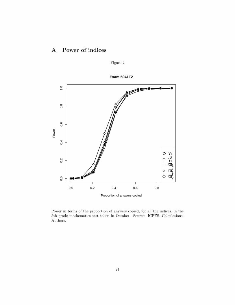
A Power of indices

Figure 2

● ● ●

●

●

●

●

●● ● ●

0.0 0.2 0.4 0.6 0.8

0.0

0.2

0.4

0.6

0.8

1.0

Exam 5041F2


Pow

er

● γ1

γ1s

ω1

ω1s

ω2s

Power in terms of the proportion of answers copied, for all the indices, in the5th grade mathematics test taken in October. Source: ICFES. Calculations:Authors.

21

Figure 3

● ●●

●

●

●

● ● ●

0.0 0.2 0.4 0.6 0.8 1.0

0.0

0.2

0.4

0.6

0.8

1.0

Exam 5042F1


Pow

er

● γ1

γ1s

ω1

ω1s

ω2s

Power in terms of the proportion of answers copied, for all the indices, in the5th grade language test taken in May. Source: ICFES. Calculations: Authors.

22

Figure 4

● ●●

●

●

●

● ● ●

0.0 0.2 0.4 0.6 0.8 1.0

0.0

0.2

0.4

0.6

0.8

1.0

Exam 5042F2


Pow

er

● γ1

γ1s

ω1

ω1s

ω2s

Power in terms of the proportion of answers copied, for all the indices, in the 5thgrade language test taken in October. Source: ICFES. Calculations: Authors.

23

Figure 5

● ● ●

●

●

●

●

● ● ● ●

0.0 0.2 0.4 0.6 0.8

0.0

0.2

0.4

0.6

0.8

1.0

Exam 5043F1


Pow

er

● γ1

γ1s

ω1

ω1s

ω2s

Power in terms of the proportion of answers copied, for all the indices, in the5th grade science test taken in May. Source: ICFES. Calculations: Authors.

24

Figure 6

● ● ●

●

●

●

●● ● ● ●

0.0 0.2 0.4 0.6 0.8

0.0

0.2

0.4

0.6

0.8

1.0

Exam 5043F2


Pow

er

● γ1

γ1s

ω1

ω1s

ω2s

Power in terms of the proportion of answers copied, for all the indices, in the5th grade science test taken in October. Source: ICFES. Calculations: Authors.

25

Figure 7

● ●●

●

●

●

●

● ● ● ● ●

0.0 0.2 0.4 0.6 0.8

0.0

0.2

0.4

0.6

0.8

1.0

Exam 9041F1


Pow

er

● γ1

γ1s

ω1

ω1s

ω2s


26

Figure 8

● ●●

●

●

●

●● ● ● ● ●

0.0 0.2 0.4 0.6 0.8

0.0

0.2

0.4

0.6

0.8

1.0

Exam 9041F2


Pow

er

● γ1

γ1s

ω1

ω1s

ω2s


27

Figure 9

● ● ●

●

●

●

●

●● ● ● ●

0.0 0.2 0.4 0.6 0.8

0.0

0.2

0.4

0.6

0.8

1.0

Exam 9042F1


Pow

er

● γ1

γ1s

ω1

ω1s

ω2s


28

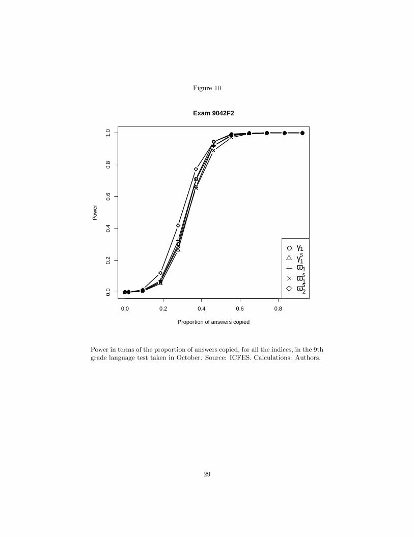
Figure 10

● ● ●

●

●

●

●

● ● ● ● ●

0.0 0.2 0.4 0.6 0.8

0.0

0.2

0.4

0.6

0.8

1.0

Exam 9042F2


Pow

er

● γ1

γ1s

ω1

ω1s

ω2s


29

Figure 11

● ●●

●

●

●

●

● ● ● ● ●

0.0 0.2 0.4 0.6 0.8

0.0

0.2

0.4

0.6

0.8

1.0

Exam 9043F1


Pow

er

● γ1

γ1s

ω1

ω1s

ω2s


30

Figure 12

● ●●

●

●

●

●● ● ● ● ●

0.0 0.2 0.4 0.6 0.8

0.0

0.2

0.4

0.6

0.8

1.0

Exam 9043F2


Pow

er

● γ1

γ1s

ω1

ω1s

ω2s


B Robustness to the number of questions

Since different tests have different quantities of questions, this could potentiallylead to different results since the standardized indices converge to a normaldistribution as the number of questions goes to infinity. In this section wepresent the results of randomly sampling 36 questions (the minimum numberof questions across all 12 exams) from each exam and repeating the exerciseoutline in Section 5. As before, a size (α) of 0.1% is used and the power of theindex is calculated at copying levels (k) of 1, 5, 10, 15, 20, ..., N , where N is thenumber of questions in the exam. To make the results as comparable as possible

31

and reduce the noise generated by using different random draws, the 100,000pairs are selected first and then the different indices are applied to the same setof randomly generated pairs.

B.1 Type I error rate

As can be seen in tables 4 and 5 the γ2, γs2 , and ω2 indices have an empiricaltype I error rate that is consistently above the theoretical type I error rate ofone in a thousand. The γ1 index (which is identical to the index developed byWesolowsky (2000)) empirical error rate is above the theoretical one in severalcases.

As before, the γ2, γs2 and ω2 indices consistently (for more than half of theexams) have an empirical type I error rate that exceeds the theoretical type Ierror rate of one in a thousand. We can also see that thee γ1 index (which isthe exact index developed by Wesolowsky (2000)) empirical error rate is abovethe theoretical one in several cases. In other words, the empirical type I errorrate results are not very sensitive to the length of the test.

32

Table 4: Type I error for the γ indices

Exam Subject Grade Month γ1 γ2 γs1 γs25041F1 Math 5th May 0.73 4.85∗∗∗ 0.4 0.87

(0.09) (0.22) (0.06) (0.09)5041F2 Math 5th October 0.97 3.88∗∗∗ 0.64 1.16∗

(0.1) (0.2) (0.08) (0.11)5042F1 Language 5th May 1.01 2.09∗∗∗ 0.63 1.04

(0.1) (0.14) (0.08) (0.1)5042F2 Language 5th October 1.4∗∗∗ 2.33∗∗∗ 1.02 1.45∗∗∗

(0.12) (0.15) (0.1) (0.12)5043F1 Science 5th May 1.52∗∗∗ 2.95∗∗∗ 1 1.6∗∗∗

(0.12) (0.17) (0.1) (0.13)5043F2 Science 5th October 0.8 1.93∗∗∗ 0.54 1.17∗

(0.09) (0.14) (0.07) (0.11)9041F1 Math 9th May 1.29∗∗∗ 2.5∗∗∗ 0.79 1.21∗∗

(0.11) (0.16) (0.09) (0.11)9041F2 Math 9th October 1.55∗∗∗ 2.21∗∗∗ 1.07 1.3∗∗∗

(0.12) (0.15) (0.1) (0.11)9042F1 Language 9th May 0.72 2.26∗∗∗ 0.34 0.97

(0.08) (0.15) (0.06) (0.1)9042F2 Language 9th October 0.81 2.1∗∗∗ 0.54 1.24∗∗

(0.09) (0.14) (0.07) (0.11)9043F1 Science 9th May 1.28∗∗∗ 2.27∗∗∗ 0.87 1.26∗∗

(0.11) (0.15) (0.09) (0.11)9043F2 Science 9th October 1.03 1.9∗∗∗ 0.65 1.21∗∗


33

Table 5: Type I error for the ω indices

Exam Subject Grade Month ω1 ω2 ωs1 ωs25041F1 Math 5th May 0.47 1.52∗∗∗ 0.2 0.62

(0.07) (0.12) (0.04) (0.08)5041F2 Math 5th October 0.84 1.51∗∗∗ 0.41 0.84

(0.09) (0.12) (0.06) (0.09)5042F1 Language 5th May 0.66 1.52∗∗∗ 0.44 0.65


(0.09) (0.13) (0.08) (0.1)5043F1 Science 5th May 0.9 1.93∗∗∗ 0.59 1.02


(0.08) (0.12) (0.07) (0.09)9041F1 Math 9th May 0.76 1.56∗∗∗ 0.43 0.93

(0.09) (0.12) (0.07) (0.1)9041F2 Math 9th October 0.93 1.37∗∗∗ 0.57 0.76

0.55 1.51∗∗∗ 0.22 0.739042F1 Language 9th May 0.55 1.51∗∗∗ 0.22 0.73


(0.09) (0.12) (0.06) (0.1)9043F1 Science 9th May 0.74 1.48∗∗∗ 0.44 0.78



B.2 Power of indices

The following figures show how powerful the γ1, γs1 , ω1, ωs1 and ωs2 indices are.Note that the ωs2 index is the most powerful for all levels of answer copying.This is true for all exams as shown in figures 13-24.

34

Figure 13

● ●●

●

●

●

●

● ●

0.0 0.2 0.4 0.6 0.8 1.0

0.0

0.2

0.4

0.6

0.8

1.0

Exam 5041F1


Pow

er

● γ1

γ1s

ω1

ω1s

ω2s


35

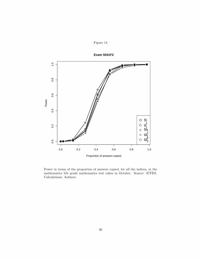
Figure 14

● ●●

●

●

●

●● ●

0.0 0.2 0.4 0.6 0.8 1.0

0.0

0.2

0.4

0.6

0.8

1.0

Exam 5041F2


Pow

er

● γ1

γ1s

ω1

ω1s

ω2s

Power in terms of the proportion of answers copied, for all the indices, in themathematics 5th grade mathematics test taken in October. Source: ICFES.Calculations: Authors.

36

Figure 15

● ●●

●

●

●

● ● ●

0.0 0.2 0.4 0.6 0.8 1.0

0.0

0.2

0.4

0.6

0.8

1.0

Exam 5042F1


Pow

er

● γ1

γ1s

ω1

ω1s

ω2s


37

Figure 16

● ●●

●

●

●

● ● ●

0.0 0.2 0.4 0.6 0.8 1.0

0.0

0.2

0.4

0.6

0.8

1.0

Exam 5042F2


Pow

er

● γ1

γ1s

ω1

ω1s

ω2s


38

Figure 17

● ●●

●

●

●

● ● ●

0.0 0.2 0.4 0.6 0.8 1.0

0.0

0.2

0.4

0.6

0.8

1.0

Exam 5043F1


Pow

er

● γ1

γ1s

ω1

ω1s

ω2s


39

Figure 18

● ●●

●

●

●

● ● ●

0.0 0.2 0.4 0.6 0.8 1.0

0.0

0.2

0.4

0.6

0.8

1.0

Exam 5043F2


Pow

er

● γ1

γ1s

ω1

ω1s

ω2s


40

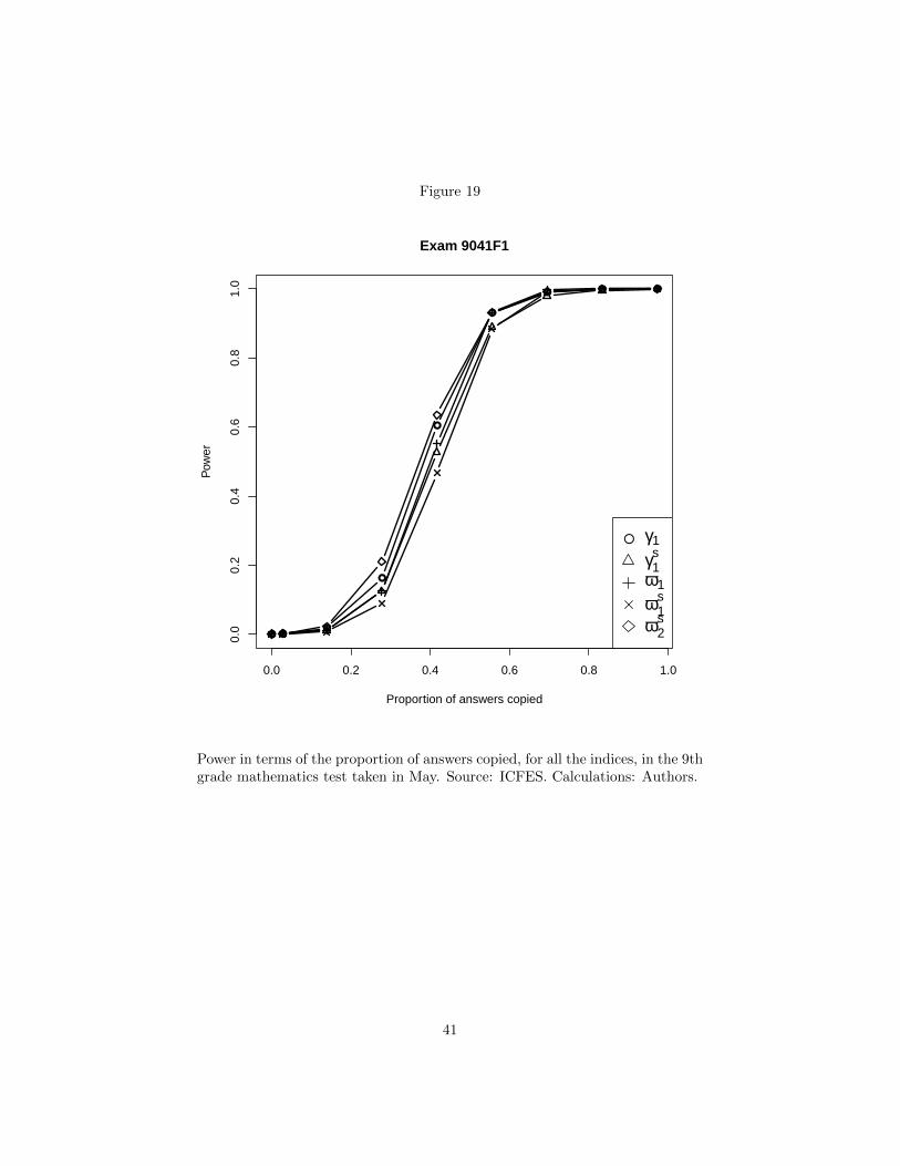
Figure 19

● ●●

●

●

●

● ● ●

0.0 0.2 0.4 0.6 0.8 1.0

0.0

0.2

0.4

0.6

0.8

1.0

Exam 9041F1


Pow

er

● γ1

γ1s

ω1

ω1s

ω2s


41

Figure 20

● ●●

●

●

●

● ● ●

0.0 0.2 0.4 0.6 0.8 1.0

0.0

0.2

0.4

0.6

0.8

1.0

Exam 9041F2


Pow

er

● γ1

γ1s

ω1

ω1s

ω2s


42

Figure 21

● ● ●

●

●

●

●● ●

0.0 0.2 0.4 0.6 0.8 1.0

0.0

0.2

0.4

0.6

0.8

1.0

Exam 9042F1


Pow

er

● γ1

γ1s

ω1

ω1s

ω2s


43

Figure 22

● ●●

●

●

●

● ● ●

0.0 0.2 0.4 0.6 0.8 1.0

0.0

0.2

0.4

0.6

0.8

1.0

Exam 9042F2


Pow

er

● γ1

γ1s

ω1

ω1s

ω2s


44

Figure 23

● ●●

●

●

●

● ● ●

0.0 0.2 0.4 0.6 0.8 1.0

0.0

0.2

0.4

0.6

0.8

1.0

Exam 9043F1


Pow

er

● γ1

γ1s

ω1

ω1s

ω2s


45

Figure 24

● ●●

●

●

●● ● ●

0.0 0.2 0.4 0.6 0.8 1.0

0.0

0.2

0.4

0.6

0.8

1.0

Exam 9043F2


Pow

er

● γ1

γ1s

ω1

ω1s

ω2s


46

on the optimality of answer-copying indices: theory and...

Documents