on the numerical simulation of unsteady solutions …nummeth/boussinesq/talk.pdf · on the...

On the Numerical Simulation of Unsteady Solutionsfor the 2D Boussinesq Paradigm Equation

Christo I. Christov

Dept. of Mathematics, University of Louisiana at Lafayette, USA

Natalia Kolkovska, Daniela VasilevaInstitute of Mathematics and Informatics, Bulgarian Academy of Sciences

1. Motivation

2. Numerical Method

3. Numerical Results

4. Conclusions and Future Work

Motivation

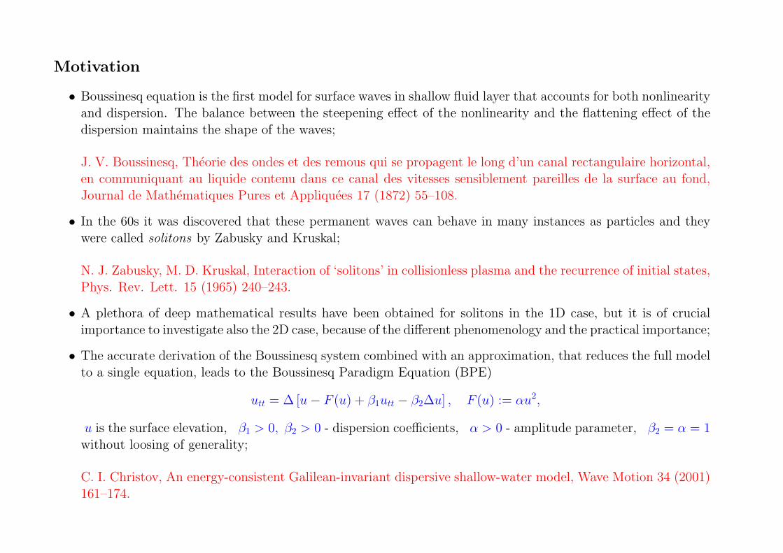
• Boussinesq equation is the first model for surface waves in shallow fluid layer that accounts for both nonlinearityand dispersion. The balance between the steepening effect of the nonlinearity and the flattening effect of thedispersion maintains the shape of the waves;

J. V. Boussinesq, Theorie des ondes et des remous qui se propagent le long d’un canal rectangulaire horizontal,en communiquant au liquide contenu dans ce canal des vitesses sensiblement pareilles de la surface au fond,Journal de Mathematiques Pures et Appliquees 17 (1872) 55–108.

• In the 60s it was discovered that these permanent waves can behave in many instances as particles and theywere called solitons by Zabusky and Kruskal;

N. J. Zabusky, M. D. Kruskal, Interaction of ‘solitons’ in collisionless plasma and the recurrence of initial states,Phys. Rev. Lett. 15 (1965) 240–243.

• A plethora of deep mathematical results have been obtained for solitons in the 1D case, but it is of crucialimportance to investigate also the 2D case, because of the different phenomenology and the practical importance;

• The accurate derivation of the Boussinesq system combined with an approximation, that reduces the full modelto a single equation, leads to the Boussinesq Paradigm Equation (BPE)

utt = ∆ [u− F (u) + β1utt − β2∆u] , F (u) := αu2,

u is the surface elevation, β1 > 0, β2 > 0 - dispersion coefficients, α > 0 - amplitude parameter, β2 = α = 1without loosing of generality;

C. I. Christov, An energy-consistent Galilean-invariant dispersive shallow-water model, Wave Motion 34 (2001)161–174.

• 2D BPE admits stationary translating soliton solutions, which can be constructed using either finite differences,perturbation technique, or Galerkin spectral method;

M. A. Christou, C. I. Christov, Fourier-Galerkin method for 2D solitons of Boussinesq equation, Math. Comput.Simul. 74 (2007) 82–92.

J. Choudhury, C. I. Christov, 2D solitary waves of Boussinesq equation, in: “ISIS International Symposiumon Interdisciplinary Science”, Natchitoches, October 6-8, 2004, APS Conference Proceedings 755, WashingtonD.C., 2005, pp. 85–90.

C. I. Christov, J. Choudhury, Perturbation solution for the 2D shallow-water waves, Mech. Res. Commun.Submitted.

C. I. Christov, Numerical implementation of the asymptotic boundary conditions for steadily propagating 2dsolitons of Boussinesq type equations, Math. Comp. Simulat. Accepted.

• Virtually nothing is known about the properties of these solutions when they are allowed to evolve in time andit is of utmost importance to answer the questions about their structural stability, i.e., what is their behaviourwhen used as initial conditions for time-dependent computations of the Boussinesq equation;

• To obtain reliable knowlegde about the time evolution of the stationary soliton solutions, it is imperative todevelop different techniques for solving of the unsteady 2D BPE;

• Some preliminary results in

A. Chertock, C. I. Christov, A. Kurganov, Central-upwind schemes for the Boussinesq paradigm equation,to appear in Proc. 4th Russian-German Advanced Research Workshop on Computational Science and HighPerformance Computing, 2010.

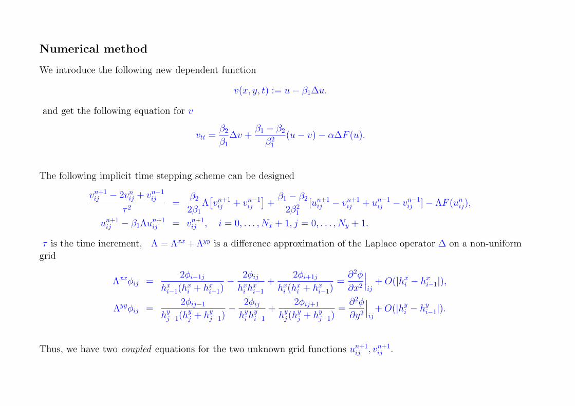
Numerical method

We introduce the following new dependent function

v(x, y, t) := u− β1∆u.

and get the following equation for v

vtt =β2

β1∆v +

β1 − β2

β21

(u− v)− α∆F (u).

The following implicit time stepping scheme can be designed

vn+1ij − 2vn

ij + vn−1ij

τ 2 =β2

2β1Λ

[vn+1

ij + vn−1ij

]+

β1 − β2

2β21

[un+1ij − vn+1

ij + un−1ij − vn−1

ij ]− ΛF (unij),

un+1ij − β1Λun+1

ij = vn+1ij , i = 0, . . . , Nx + 1, j = 0, . . . , Ny + 1.

τ is the time increment, Λ = Λxx + Λyy is a difference approximation of the Laplace operator ∆ on a non-uniformgrid

Λxxφij =2φi−1j

hxi−1(h

xi + hx

i−1)− 2φij

hxi h

xi−1

+2φi+1j

hxi (h

xi + hx

i−1)=

∂2φ

∂x2

∣∣∣ij

+ O(|hxi − hx

i−1|),

Λyyφij =2φij−1

hyj−1(h

yj + hy

j−1)− 2φij

hyi h

yi−1

+2φij+1

hyj(h

yj + hy

j−1)=

∂2φ

∂y2

∣∣∣ij

+ O(|hyi − hy

i−1|).

Thus, we have two coupled equations for the two unknown grid functions un+1ij , vn+1

ij .

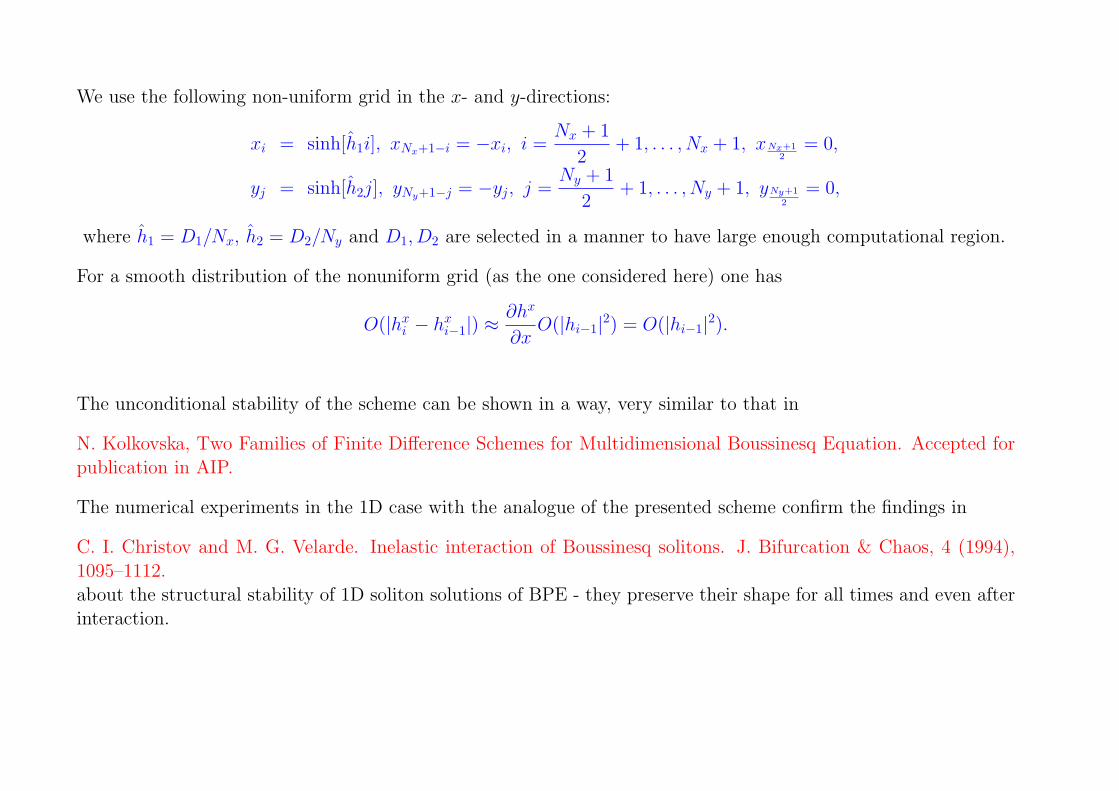
We use the following non-uniform grid in the x- and y-directions:

xi = sinh[h1i], xNx+1−i = −xi, i =Nx + 1

2+ 1, . . . , Nx + 1, xNx+1

2= 0,

yj = sinh[h2j], yNy+1−j = −yj, j =Ny + 1

2+ 1, . . . , Ny + 1, yNy+1

2= 0,

where h1 = D1/Nx, h2 = D2/Ny and D1, D2 are selected in a manner to have large enough computational region.

For a smooth distribution of the nonuniform grid (as the one considered here) one has

O(|hxi − hx

i−1|) ≈∂hx

∂xO(|hi−1|2) = O(|hi−1|2).

The unconditional stability of the scheme can be shown in a way, very similar to that in

N. Kolkovska, Two Families of Finite Difference Schemes for Multidimensional Boussinesq Equation. Accepted forpublication in AIP.

The numerical experiments in the 1D case with the analogue of the presented scheme confirm the findings in

C. I. Christov and M. G. Velarde. Inelastic interaction of Boussinesq solitons. J. Bifurcation & Chaos, 4 (1994),1095–1112.about the structural stability of 1D soliton solutions of BPE - they preserve their shape for all times and even afterinteraction.

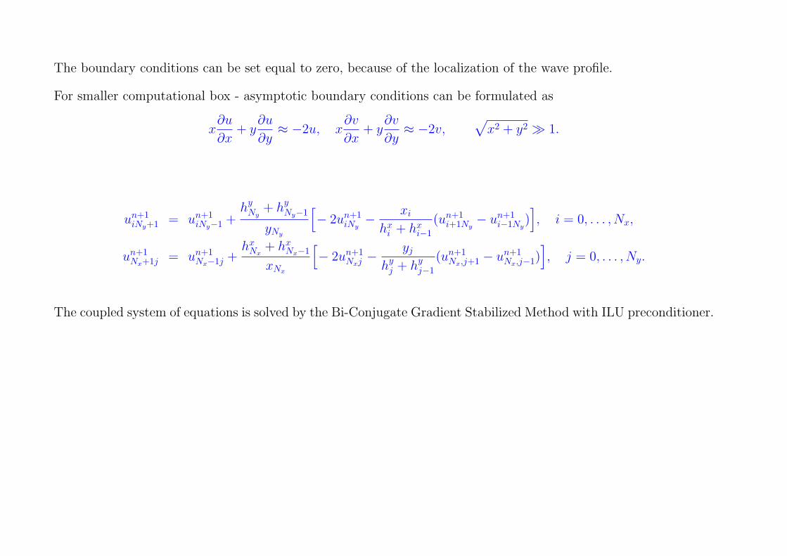
The boundary conditions can be set equal to zero, because of the localization of the wave profile.

For smaller computational box - asymptotic boundary conditions can be formulated as

x∂u

∂x+ y

∂u

∂y≈ −2u, x

∂v

∂x+ y

∂v

∂y≈ −2v,

√x2 + y2 � 1.

un+1iNy+1 = un+1

iNy−1 +hy

Ny+ hy

Ny−1

yNy

[− 2un+1

iNy− xi

hxi + hx

i−1(un+1

i+1Ny− un+1

i−1Ny)], i = 0, . . . , Nx,

un+1Nx+1j = un+1

Nx−1j +hx

Nx+ hx

Nx−1

xNx

[− 2un+1

Nxj −yj

hyj + hy

j−1(un+1

Nx,j+1 − un+1Nx,j−1)

], j = 0, . . . , Ny.

The coupled system of equations is solved by the Bi-Conjugate Gradient Stabilized Method with ILU preconditioner.

Numerical experiments

We use the following best fit approximation for the shape of the stationary propagating soliton with velocity c

C. I. Christov, J. Choudhury, Perturbation solution for the 2D shallow-water waves, Submitted to Mech. Res.Commun.

us(x, y; c) = f(x, y) + c2 [(1− β1)ga(x, y) + β1gb(x, y)] + c2 [(1− β1)h1(x, y) + β1h2(x, y)] cos(2 arctan(y/x).

f(x, y) =2.4(1 + 0.24r2)

cosh(r)(1 + 0.095r2)1.5 , ga(r) = − 1.2(1− 0.177r2.4)

cosh(r)(1 + 0.11r2.1), gb(r) = − 1.2(1 + 0.22r2)

cosh(r)(1 + 0.11r2.4),

hi(x, y) =air

2 + bir3 + cir

4 + vir6

1 + dir + eir2 + fir3 + gir4 + hir5 + qir6 + wir8 , r(x, y) =√

x2 + y2, θ(x, y) = arctan(y/x),

a1 = 1.03993, a2 = 31.2172, b1 = 6.80344, b2 = −10.0834, c1 = −0.22992, c2 = 3.97869, d1 = 12.6069, d2 = 77.9734,

e1 = 13.5074, e2 = −76.9199, f1 = 2.46495, f2 = 55.4646, g1 = 2.45953, g2 = −12.9335, h1 = 1.03734, h2 = 1.0351,

q1 = −0.0246084, q2 = 0.628801, v1 = 0.0201666, v2 = −0.0290619, w1 = 0.00408432, w2 = −0.00573272.

In the examples below us(x, y; c) for β1 = 3 is taken as initial data for t = 0 and the second initial condition maybe chosen as

∂u/∂t = −c ∂us/∂y, t = 0, or u(x, y,−τ) = us(x, y + cτ ; c).

The solutions are computed on 3 different grids in the region x, y ∈ [−50, 50] (with 161 × 161, 321 × 321 and641 × 641 grid points), with at least 3 different time steps (τ = 0.2, 0.1 and 0.05), with or without using somesymmetry conditions at x = 0 (and y = 0 for c = 0), and using zero or asymptotic boundary conditions.

Example 1. c = 0 – the profile of the initial condition is a standing soliton. The nonlinearity is not strong enoughand the solution transforms into a propagating cylindrical wave, similar to the one generated on a water surfacewhen an object is dropped into it. The behaviour of the solution is one and the same on all grids, for all times steps,and does not depend on the type of the boundary conditions used.

−10 −8 −6 −4 −2 0 2 4 6 8 10

0

0.5

1

1.5

2

2.5

y

u

cross section x=0

t=0t=4t=8t=12t=16t=20

0 2 4 6 8 10 12 14 16 18 200

0.5

1

1.5

2

2.5

t

u max

maximum of the solution

3212 grid points, τ=0.1





3212 grid points, τ=0.1,asympt.b.c.

Figure 1: Evolution of the solution for c = 0 – its shape for x = 0 and the values of the maximum

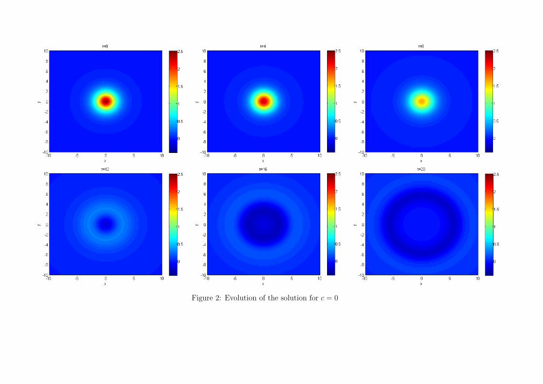
Figure 2: Evolution of the solution for c = 0

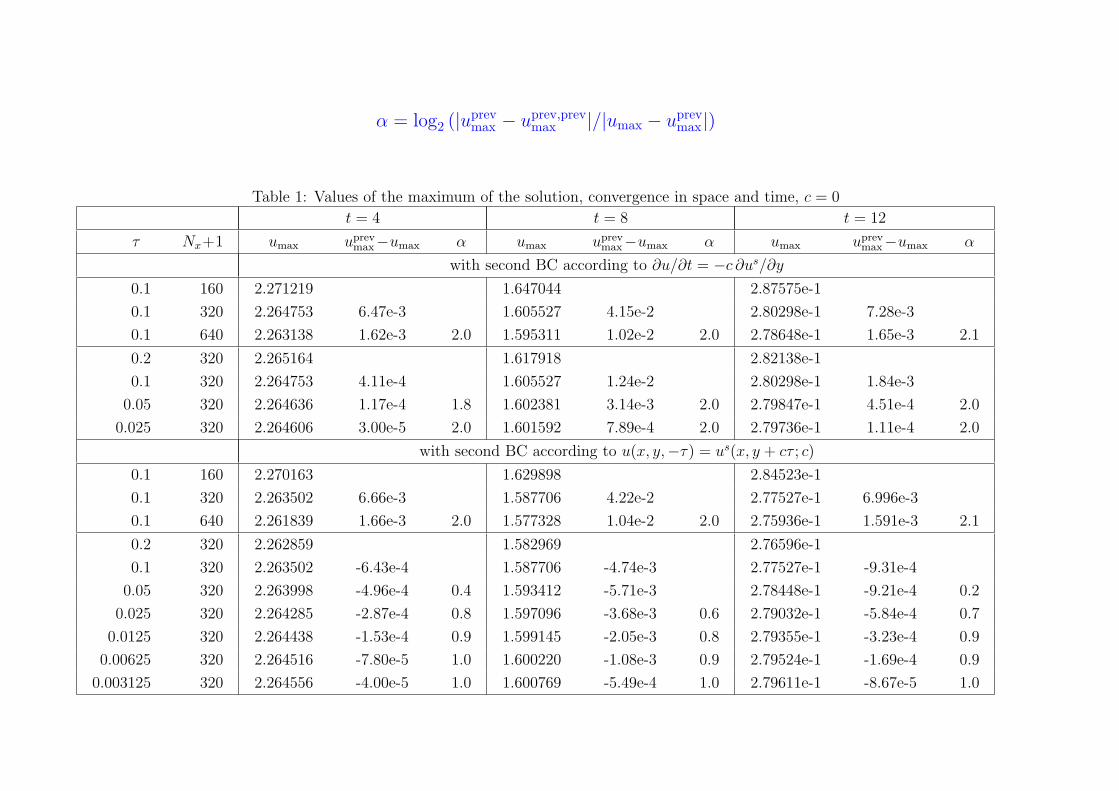
α = log2 (|uprevmax − uprev,prev

max |/|umax − uprevmax |)

Table 1: Values of the maximum of the solution, convergence in space and time, c = 0

t = 4 t = 8 t = 12

τ Nx+1 umax uprevmax−umax α umax uprev

max−umax α umax uprevmax−umax α

with second BC according to ∂u/∂t = −c ∂us/∂y

0.1 160 2.271219 1.647044 2.87575e-1

0.1 320 2.264753 6.47e-3 1.605527 4.15e-2 2.80298e-1 7.28e-3

0.1 640 2.263138 1.62e-3 2.0 1.595311 1.02e-2 2.0 2.78648e-1 1.65e-3 2.1

0.2 320 2.265164 1.617918 2.82138e-1

0.1 320 2.264753 4.11e-4 1.605527 1.24e-2 2.80298e-1 1.84e-3

0.05 320 2.264636 1.17e-4 1.8 1.602381 3.14e-3 2.0 2.79847e-1 4.51e-4 2.0

0.025 320 2.264606 3.00e-5 2.0 1.601592 7.89e-4 2.0 2.79736e-1 1.11e-4 2.0

with second BC according to u(x, y,−τ) = us(x, y + cτ ; c)

0.1 160 2.270163 1.629898 2.84523e-1

0.1 320 2.263502 6.66e-3 1.587706 4.22e-2 2.77527e-1 6.996e-3

0.1 640 2.261839 1.66e-3 2.0 1.577328 1.04e-2 2.0 2.75936e-1 1.591e-3 2.1

0.2 320 2.262859 1.582969 2.76596e-1

0.1 320 2.263502 -6.43e-4 1.587706 -4.74e-3 2.77527e-1 -9.31e-4

0.05 320 2.263998 -4.96e-4 0.4 1.593412 -5.71e-3 2.78448e-1 -9.21e-4 0.2

0.025 320 2.264285 -2.87e-4 0.8 1.597096 -3.68e-3 0.6 2.79032e-1 -5.84e-4 0.7

0.0125 320 2.264438 -1.53e-4 0.9 1.599145 -2.05e-3 0.8 2.79355e-1 -3.23e-4 0.9

0.00625 320 2.264516 -7.80e-5 1.0 1.600220 -1.08e-3 0.9 2.79524e-1 -1.69e-4 0.9

0.003125 320 2.264556 -4.00e-5 1.0 1.600769 -5.49e-4 1.0 2.79611e-1 -8.67e-5 1.0

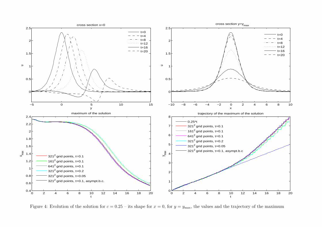
Example 2. The next case is for a phase speed c = 0.25. For t < 8 the soliton not only moves with a speed, closeto c = 0.25, but also behaves like a soliton, i.e., preserves its shape, although its maximum slightly decreases. Forlarger times the solution transforms into a diverging propagating wave, but without a cylindrical symmetry becauseof the propagation of the wave.

Figure 3: Evolution of the solution for c = 0.25

−5 0 5 10 15

0

0.5

1

1.5

2

2.5

y

ucross section x=0

t=0t=4t=8t=12t=16t=20

−10 −8 −6 −4 −2 0 2 4 6 8 10

0

0.5

1

1.5

2

2.5

x

u

cross section y=ymax

t=0t=4t=8t=12t=16t=20

0 2 4 6 8 10 12 14 16 18 200.4

0.6

0.8

1

1.2

1.4

1.6

1.8

2

2.2

2.4

t

u max







3212 grid points, τ=0.1, asympt.b.c.

0 2 4 6 8 10 12 14 16 18 200

1

2

3

4

5

6

7

8

t

y max

trajectory of the maximum of the solution

0.25*t






3212 grid points, τ=0.1, asympt.b.c

Figure 4: Evolution of the solution for c = 0.25 – its shape for x = 0, for y = ymax, the values and the trajectory of the maximum

Table 2: Values of the maximum of the solution, convergence in space and time, c = 0.25

t = 4 t = 8 t = 12




0.1 160 2.261156 2.191684 1.725273

0.1 320 2.257642 3.51e-3 2.165738 2.59e-2 1.639348 8.59e-2

0.1 640 2.256689 9.53e-4 1.9 2.158619 7.12e-3 1.9 1.619535 1.98e-2 2.1

0.2 320 2.268606 2.226354 1.848499

0.1 320 2.257642 1.10e-2 2.165738 6.06e-2 1.639348 2.09e-1

0.05 320 2.254871 2.77e-3 2.0 2.148196 1.75e-2 1.8 1.588800 5.05e-2 2.0

with second BC according to according to u(x, y,−τ) = us(x, y + cτ ; c)

0.1 160 2.261550 2.189987 1.718885

0.1 320 2.256804 4.75e-3 2.156155 3.38e-2 1.609205 1.10e-1

0.1 640 2.255469 1.34e-3 1.8 2.147008 9.15e-3 1.9 1.584249 2.50e-2 2.1

0.2 320 2.264348 2.195763 1.734455

0.1 320 2.256804 7.54e-3 2.156155 3.96e-2 1.609205 1.25e-1

0.05 320 2.254958 1.85e-3 2.0 2.146491 9.66e-3 2.0 1.583778 2.54e-2 2.3

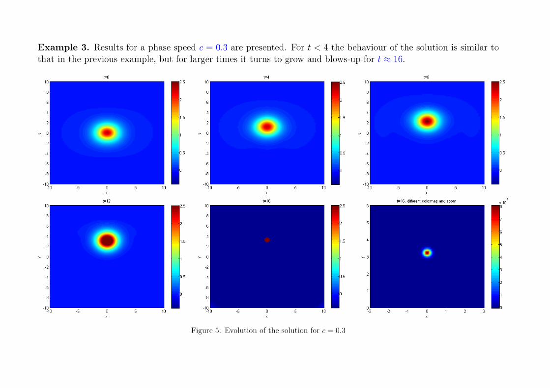
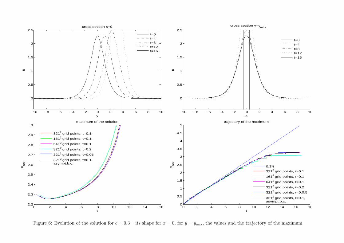
Example 3. Results for a phase speed c = 0.3 are presented. For t < 4 the behaviour of the solution is similar tothat in the previous example, but for larger times it turns to grow and blows-up for t ≈ 16.

Figure 5: Evolution of the solution for c = 0.3

−10 −8 −6 −4 −2 0 2 4 6 8 10

0

0.5

1

1.5

2

2.5

y

ucross section x=0

t=0t=4t=8t=12t=16

−10 −8 −6 −4 −2 0 2 4 6 8 10

0

0.5

1

1.5

2

2.5

x

u

cross section y=ymax

t=0t=4t=8t=12t=16

0 2 4 6 8 10 12 14 162.2

2.3

2.4

2.5

2.6

2.7

2.8

2.9

3

t

u max








0 2 4 6 8 10 12 14 16 180

0.5

1

1.5

2

2.5

3

3.5

4

4.5

5

t

y max

trajectory of the maximum

0.3*t





3212 grid points, τ=0.0.5


Figure 6: Evolution of the solution for c = 0.3 – its shape for x = 0, for y = ymax, the values and the trajectory of the maximum

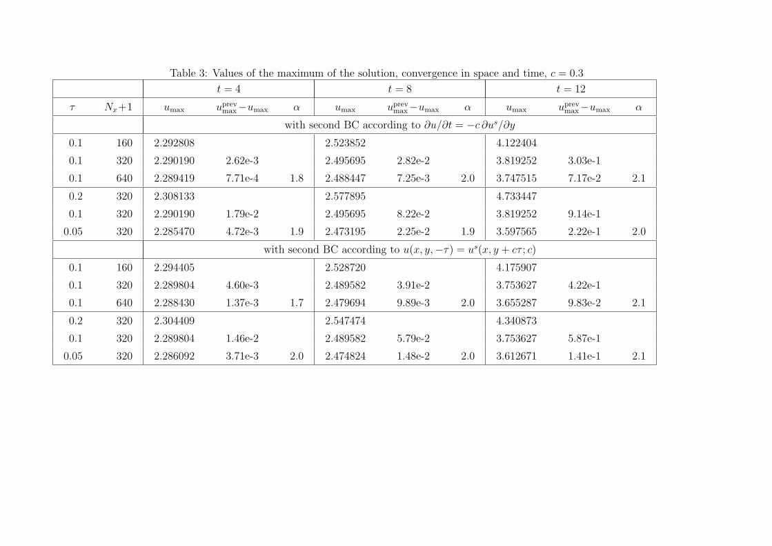
Table 3: Values of the maximum of the solution, convergence in space and time, c = 0.3

t = 4 t = 8 t = 12




0.1 160 2.292808 2.523852 4.122404

0.1 320 2.290190 2.62e-3 2.495695 2.82e-2 3.819252 3.03e-1

0.1 640 2.289419 7.71e-4 1.8 2.488447 7.25e-3 2.0 3.747515 7.17e-2 2.1

0.2 320 2.308133 2.577895 4.733447

0.1 320 2.290190 1.79e-2 2.495695 8.22e-2 3.819252 9.14e-1

0.05 320 2.285470 4.72e-3 1.9 2.473195 2.25e-2 1.9 3.597565 2.22e-1 2.0

with second BC according to u(x, y,−τ) = us(x, y + cτ ; c)

0.1 160 2.294405 2.528720 4.175907

0.1 320 2.289804 4.60e-3 2.489582 3.91e-2 3.753627 4.22e-1

0.1 640 2.288430 1.37e-3 1.7 2.479694 9.89e-3 2.0 3.655287 9.83e-2 2.1

0.2 320 2.304409 2.547474 4.340873

0.1 320 2.289804 1.46e-2 2.489582 5.79e-2 3.753627 5.87e-1

0.05 320 2.286092 3.71e-3 2.0 2.474824 1.48e-2 2.0 3.612671 1.41e-1 2.1

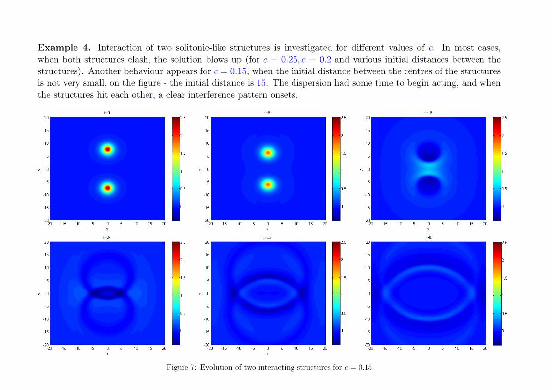
Example 4. Interaction of two solitonic-like structures is investigated for different values of c. In most cases,when both structures clash, the solution blows up (for c = 0.25, c = 0.2 and various initial distances between thestructures). Another behaviour appears for c = 0.15, when the initial distance between the centres of the structuresis not very small, on the figure - the initial distance is 15. The dispersion had some time to begin acting, and whenthe structures hit each other, a clear interference pattern onsets.

Figure 7: Evolution of two interacting structures for c = 0.15

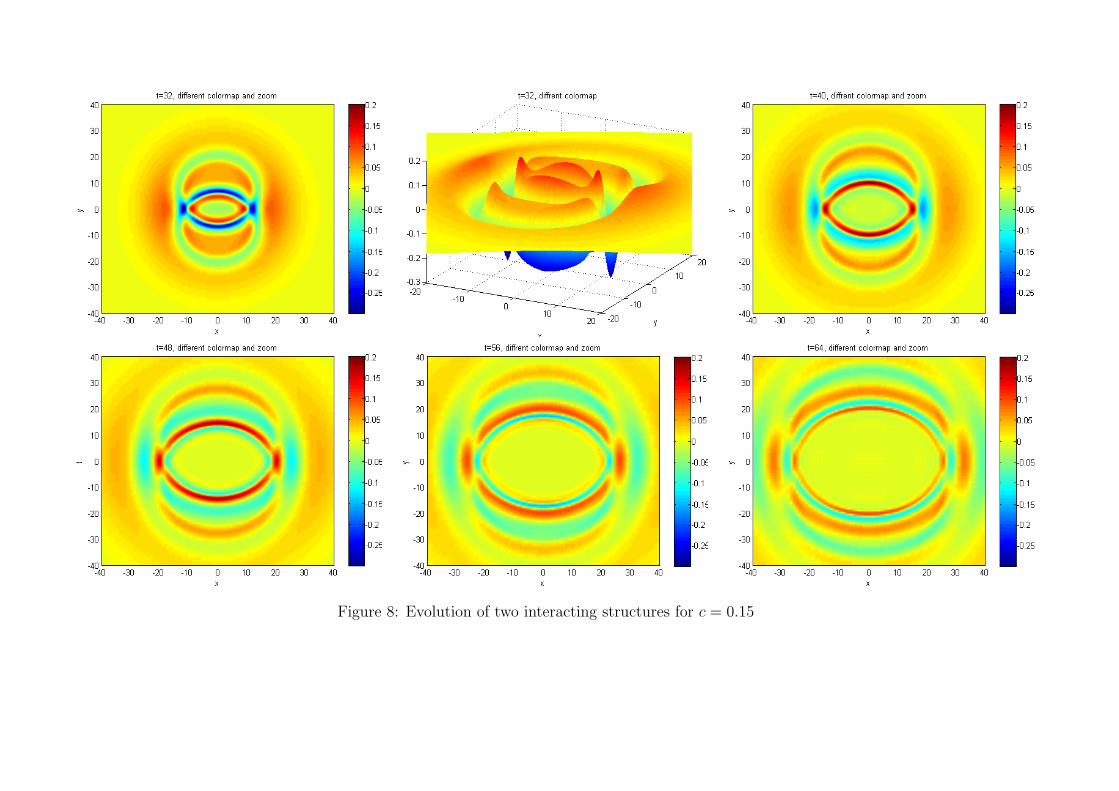
Figure 8: Evolution of two interacting structures for c = 0.15

Conclusion

• Our results are very close to the results of Chertock, Christov and Kurganov from

A. Chertock, C. I. Christov, A. Kurganov, Central-upwind schemes for the Boussinesq paradigm equation,to appear in Proc. 4th Russian-German Advanced Research Workshop on Computational Science and HighPerformance Computing, 2010.

and confirm the solitonic-like behaviour of the solutions for relatively small times.

• Unfortunately, the investigated solutions are not structurally stable and transform either in diverging propa-gating waves or blow-up.

• For c ≈ 0.3, an time interval exists in which the solution is virtually preserving its shape whils steadilytranslating means that 2D solitons could be found for equations from the class of the BPE. This means thatthe nonlinearity is strong enough to balance the dispersion which is now much stronger than in the 1D case.

• Probably, the quadratic nonlinearity in BPE is not enough for modeling permanent soliton-like waves. Ourfuture plans include experiments with different types of nonlinearities in the source term and in the coefficientsof the equation, as well as development of faster solvers for the linear systems, arising after the discretization.

on the numerical simulation of unsteady solutions …nummeth/boussinesq/talk.pdf · on the...

Documents