on the micrometeorology of the southern great plains 1: legacy relationships revisited

Boundary-Layer Meteorol (2014) 151:389–405DOI 10.1007/s10546-013-9902-2

ARTICLE

On the Micrometeorology of the Southern Great Plains 1:Legacy Relationships Revisited

B. B. Hicks · W. R. Pendergrass III · C. A. Vogel ·R. N. Keener Jr. · S. M. Leyton

Received: 30 July 2013 / Accepted: 23 December 2013 / Published online: 29 January 2014© Springer Science+Business Media Dordrecht 2014

Abstract Data from a 32-m tower located near Ocotillo, Texas (32.12050◦N; 101.37555◦W),provide an opportunity to examine the relevance of standard micrometeorological flux–gradient formulations to observations made in an area characteristic of a large portion ofthe central USA, within the Southern Great Plains. Comparison with data obtained at agreater height (80 m) reveals that the velocity distributions change substantially betweenthe lower set of observations and the upper, with the former being constrained at the lowwind-speed end. In the early morning, sensible heat-flux divergence correlates well with themeasured rate of change of temperature with time within the surface layer of air sampled bythe tower, but this association disappears when the depth of the mixed layer extends beyondthe reach of the tower. As in the case of all previous examinations of flux–gradient relation-ships, the overall dependence of the dimensionless wind and temperature gradients φm andφH on stability is characterized by considerable scatter, with the familiar relationships bestdescribing the average. For conditions of stable stratification, there is indeed the expectedclose proximity of φm and φH, however, describing either φm or φH in terms of the classicalstability index Z/L (where Z is the height above the zero plane and L is the Obukhov lengthscale of turbulence) then appears questionable because the dependence ofφm on the measuredsensible heat flux is not always single-valued, especially near the surface. For unstable strati-fication, support is found for the conclusions of early workers that free convection initiates atabout Z/L ≈ −0.03, and that the general behaviour is then compatible with the concept of amoving air mass from which momentum is continuously extracted, embedded within freely

B. B. Hicks (B)MetCorps, P. O. Box 1510, Norris, TN 37828, USAe-mail: [email protected]

W. R. Pendergrass III · C. A. VogelNOAA/ARL/ATDD, P. O. Box 2456, Oak Ridge, TN 37831, USA

C. A. VogelOak Ridge Associated Universities, P. O. Box 117, Oak Ridge, TN 37831, USA

R. N. Keener Jr. · S. M. LeytonDuke Energy, 26 South Church Street, Charlotte, NC 28202, USA

123

390 B. B. Hicks et al.

convective cells. It is concluded that legacy descriptions of the relationships between fluxesand gradients apply to averages that might occur rarely, that a dominant factor is likely thechaotic nature of the processes that control the variables considered in these relationships,and that the net consequence of the original randomness is that the levels of predictabilitytheoretically attainable might never be realized in practice.

Keywords Dimensional analysis · Fluxes · Normalization · Sunrise · Thermal stability ·Vertical gradients

1 Introduction

A central problem for micrometeorologists has been to relate air–surface exchange ratesof momentum, heat, water vapour, carbon dioxide and (increasingly) various pollutants toquantities that can be predicted with confidence or extracted from available data sources. Theflux–gradient formulations (involving the dependence on stability of the φ-functions, definedas φm = (∂u/∂Z)/(u∗/(k Z)) and φH = (∂θ/∂Z)/(H/(ρcpku∗)) are intended to facilitatethis process, with their application often making use of the height integrals of the φ-functions(the ψ-functions). Here u is the wind speed at height Z above the relevant zero plane, u∗is the friction velocity, k is the von Karman constant, θ is potential temperature, H is thesensible heat flux, ρ is air density, and cp is the specific heat of air at constant pressure (seeMonin and Obukhov 1954, and any of many text books such as Plate 1971, and Garratt 1992).Many different versions of these relationships are to be found in the published literature. Nomatter what form of the relationships might be used, their significance over any short periodof time is questionable because all of these relationships are expressions describing averages,and short-term applications should include an element (perhaps dominant) of randomness orof factors external to the local surface boundary layer. In many models, the details of the φ-functions are unimportant, since their practical relevance is limited to interpolation betweenthe wind speed aloft, as determined synoptically, and the surface. There are other applications,however, in which the formulations of these relationships have a greater importance, suchas in the assessment of air–surface exchange of quantities as varied as water, carbon dioxideand air pollutants.

The widely accepted φ-functions were initially based on observations made using sensorsof an earlier time. The functions were pragmatic approximations, derived by drawing curves“of convenience” through a limited number of data points that were highly scattered, evenwhen plotted in a log–log form. The scatter of early data was such that for conditions ofunstable stratification it was possible to describe curves as

φm = (1 − α1 Z/L)−1/4 (1)

andφH = (1 − α2 Z/L)−1/2 (2)

through the experimental results, with uncertainties such that an assumption α1 = α2 (andcommonly = 15 or 16) could be accepted. A convenient consequence was that for unstablestratification the gradient Richardson number would be numerically the same as Z/L . Sub-sequent experiments refined these early relationships, and several versions appear in modernapplications. In practice, the differences among them are not major.

For stable stratification, most workers accept a log-linear expression that originates as thefirst terms of a Taylor expansion, but with some remaining disagreement about the value ofthe constant α3 (≈6) in

123

On the Micrometeorology of the Southern Great Plains 1 391

φm = 1 + α3 Z/L . (3)

There is also general acceptance thatφH will be similar (even equal) toφm in stable conditions,there being no physical process that influences one without affecting the other until thelimiting effects of very strong stability become apparent (q.v. Mahrt 2010). This impliesequivalence of φH and φm at neutral, which result has been supported by many (but not all,e.g. Businger et al. 1971) field studies. It is obvious, however, that in stable stratificationthere remains a role for buoyancy, which will then work to damp vertical displacements.

The legacy relationships (1)–(3) were initially derived using developmental instrumen-tation deployed over carefully selected areas where time stationarity and horizontal homo-geneity of both the surface and the air passing over it could be assumed (e.g. Dyer and Hicks1970). Such outdoor laboratories are rare, and it remains unclear as to how well the resultsobtained in these special circumstances apply to the “real world.” Moreover, a major questionrelates to how randomness (or chaos) affects the relationships of interest. This matter is ofdirect relevance to modern prognostic numerical models of the atmosphere, which constructforecasts by assuming the applicability of relationships among averages without (usually)acknowledging that the lower atmosphere rarely maintains an average state. In the analysisthat follows, initial attention is given to a conventional analysis of the data, paralleling themethods used in the many early experiments upon which the relationships (1) (2) and (3) werebased. Following this initial examination, several aspects of the dataset are scrutinized moreclosely, with special attention to the validity (or appropriateness) of assumptions inherent inthe conventional approach.

2 Site Details and Instrumentation

The observations considered here were obtained using a 32-m micrometeorological towerlocated at 32.12050◦N; 101.37555◦W, near Ocotillo, Texas, within a field program conductedin collaboration with Duke Energy Generation, Inc. The site constitutes the upwind region ofDuke Energy’s Ocotillo wind farm, operating 28 Suzlon wind turbines each delivering up to2.1 MW. Figure 1 shows the meteorological tower viewed from the south, showing severaldownwind wind turbines and a larger meteorological tower used to obtain wind data at 80-mheight, this being the turbine hub height. The area is part of the Southern Great Plains (seethe inset in Fig. 1), and bears the expected varieties of vegetation—mostly native grasses anda few trees, mainly mesquite. Figure 2 illustrates the site layout; the terrain is generally level,with only slight changes in elevation. It is ∼ 840 m above mean sea level.

There are three distinct levels of plant canopy within the domain of present interest. Thelowest vegetation level is composed of grasses, dominated by buffalo grass, with the grasscanopy having a coverage of roughly 70 %, and typically 0.25–0.3 m tall. The second levelconsists primarily of cactus and smaller mesquite trees, generally about 1 m high. Thisvegetation, as can be seen in Fig. 1, is quite sparse, covering <5 % of the area. The thirdcanopy level consists of larger mesquite and juniper trees, roughly 2–3 m in height covering<1 % of the total area. The remainder of the surface is barren. Daytime temperatures are quitehigh (>40 ◦C) in the summer with a large diurnal range (typically 25–30 ◦C). Temperaturesfall below 0 ◦C in autumn with the last freezing temperatures usually in mid-April. Wintersare characterized by frequent cold periods followed by rapid warming, while frontal passagesgenerally occur every 3 days.

Micrometeorological data collection started in May 2010. The principal goal was to mon-itor basic atmospheric boundary-layer meteorological mean and turbulence variables of wind

123


Fig. 1 A view from the south of the Ocotillo micrometeorological site, showing wind turbines in the distance,the meteorological tower carrying wind sensors at 80-m height, and the micrometeorological 32-m towercarrying the instrumentation currently reported. The inset shows the geographic location of the present site(the star), showing its inclusion in the red shaded area of semi-arid and short-grass pasture classically referredto as the Southern Great Plains. There are several alternative depictions of the area known as the Great Plains,with many including the area of taller grasses to the east of that shown here

speed, wind direction, and temperature at multiple levels, so as to permit examination of dif-ferent methods for assessing wind energy potential. Three-dimensional sonic anemometersand aspirated thermometers were installed on booms to provide data for seven heights—2.99,8.5, 10.0, 14.75, 17.2, 20.99, and 27.39 m. Details of the installation are given by White et al.(2014). In brief, the anemometers were R. M. Young model 81000, thermometry employedplatinum resistance sensors (from Thermometrics, Inc.) in aspirated shields, and data acquisi-tion and archiving made use of Campbell Scientific CR 1000 dataloggers with real-time datalinkage to the NOAA Oak Ridge facility via a Sierra Wireless Airlink GX4409 4g modem.

In addition to sonic anemometer velocity measurements obtained using the 32-m microm-eteorological tower, data were also available from a mechanical wind vane system at 80 m(turbine hub height), mounted on the nearby meteorological tower (the larger tower seenin Fig. 1). These 80-m data provide an intriguing insight into the local wind climatology.Figure 3 presents histograms showing the distributions of wind-speed and direction at twolevels—from the micrometeorological tower at a height of 10 m and from the wind farmmeteorological tower at 80 m. Comparison of the wind-speed histograms in Fig. 3 is reveal-ing, in that the 80-m data are approximately normally distributed, whereas the 10-m dataare not. Roughly 60 % of the observations correspond to a 30◦ direction window, centred onabout 180◦ for the 10-m data and 170◦ for the 80-m data. In this analysis, all data are used,for the period April–August 2011. However, in the following illustrations where individualpoints are plotted only 2 % of the data are used: after ordering the dataset according to the

123


Fig. 2 The layout of the site, showing the locations of the micrometeorological tower (the red cross) and ofthree of the wind turbines to the north. There is an uncharacteristic fetch to the north-east. The present analysisuses wind directions from 080◦ through north to 280◦. Developed areas serviced by dirt roads are the sites ofproducing oil wells

abscissa, every 50th point is plotted. This procedure has been adopted to show the detailsof the dataset without obscuring such details by creating a cloud of points with no obviousinternal structure, while retaining a visual indication of the scatter involved. Note that winddirection data have been corrected for magnetic declination and indicate the wind directionrelative to true north.

3 Covariance and Gradient Data

Sonic anemometers reported winds at 10 Hz frequency for heights above the ground of 2.99,8.50, 10.00, 14.75, 17.20, 20.99, and 27.39 m, with temperature gradient data derived fromaspirated platinum resistance thermometers at each level. Logistical considerations associatedwith the tower construction prohibited adoption of the usual two-fold height intervals. In thefollowing analysis, w′T ′ has been computed using the fast response temperature signalsderived from the sonic systems.

123


Fig. 3 Histograms showing the distribution of wind speed and wind direction over a four month period, atheights of 10 and 80 m

The sonic anemometers impose a slight updraft due to their physical configuration, witha large bulk below the transducer array and none above. To correct for the presence of theartifact wind streamline deformation, coordinate rotation has been imposed in computationof the w′u′ covariance, so that both the average vertical and transverse velocities are zeroin the transformed coordinate system. In the case of w′T ′, it is assumed that buoyancy iscontrolled by gravity and hence the coordinates have not been rotated. Although the validityof this remains debatable, in practice there is little difference. Recent work has indicatedthat the configuration of the sonic anemometers used here imposes an additional effect onthe determination of fluctuations in the vertical velocity (Kochendorfer et al. 2012). Theerrors then arising in the eddy-flux determinations (after coordinate rotation) are typicallyin the range of 10–12 % underestimation, and such should be considered indicative of theuncertainty associated with any of the covariances reported here. However, any resultingcorrections, if applicable, should apply to every measurement height.

Data were gathered as 15-min runs, around the clock without interruption. These dataallow an examination of the constancy of fluxes with height in the atmospheric surfacelayer. To this end, the seven independent measurements of w′T ′ and w′u′ obtained for every

15-min run have been averaged linearly to yield overall tower averages w′T ′ and w′u′.Departures from these tower averages have then been computed for each level, and used toderive overall mean departures from the average tower covariances as a function of the timeof day. These mean values are plotted in Fig. 4, and although there is considerable scatter inthe results, some consistent variations are apparent. The plots show that for two of the levelsof measurement, 2.99 and 17.2 m, there are strong diurnal signals, with major departuresthat appear to correlate with the time of day (or with the magnitude of the convective flux orperhaps the daytime temperature regime). Regardless of whether such large departures aredue to some peculiarity of the instrumentation, to site imperfections of some kind, or to someother characteristic of the prevailing surface layer, it is clear that daytime covariances from

123


Fig. 4 An examination of the variation with height of the covariances: w′T ′ (the upper panel) and w′u′ (thelower panel). The lines represent the departures from averages across all levels, for each individual 15-minrun, sorted according to time of day and then averaged in 1-h increments

these levels fall outside the range that might best be associated with a “constant-flux layer.”To explore the matter of the diurnal cycle of flux divergence in more detail would requirespatial information (vertical, as well as horizontal) that is lacking, and would also requireconsideration of longer averaging times.

The small departures apparent for nighttime cases in Fig. 4 appear reassuring, but it shouldbe remembered that the actual fluxes at night are small and hence the values plotted are notnecessarily indicative of improved performance at night.

A familiar guideline concerning the constant-flux layer is that the lower bound is at aheight of about d + 10z0. Using the values obtained and discussed below (roughness lengthz0 ≈ 0.18 ± 0.02 m, displacement height d ≈ 0.8 ± 0.4 m), this would indicate a lower levelof about 2.6 m. Thus the 2.99-m data from the present tower should be considered with somecaution. Close examination of the data reveals that the wind speed and momentum flux dataare particularly affected by upwind irregularities or obstacles (as are obvious in Fig. 1), theconsequences of which become evident in a detailed study of variations with wind direction(which are not apparent in data from higher levels). The temperature covariance data are notso affected. There is no corresponding potential explanation for the behaviour of the 17.2 msystem, thus the cause is suspected to have been instrumental.

In Fig. 5, differences inw′T ′ from 2.99 to 27.39 m are plotted (as the quantity�w′T ′/�z)against the time of day relative to sunrise. Also plotted is an indicator of the heat storage rate

123


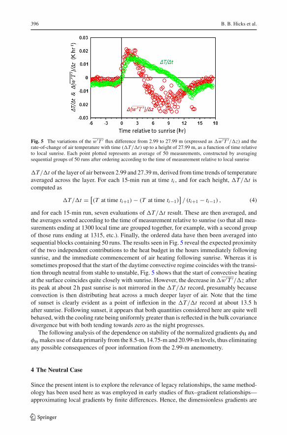
Fig. 5 The variations of the w′T ′ flux difference from 2.99 to 27.99 m (expressed as �w′T ′/�z) and therate-of-change of air temperature with time (�T/�t) up to a height of 27.99 m, as a function of time relativeto local sunrise. Each point plotted represents an average of 50 measurements, constructed by averagingsequential groups of 50 runs after ordering according to the time of measurement relative to local sunrise

�T/�t of the layer of air between 2.99 and 27.39 m, derived from time trends of temperatureaveraged across the layer. For each 15-min run at time ti , and for each height, �T/�t iscomputed as

�T/�t = [(T at time ti+1)− (T at time ti−1)

]/ (ti+1 − ti−1) , (4)

and for each 15-min run, seven evaluations of �T/�t result. These are then averaged, andthe averages sorted according to the time of measurement relative to sunrise (so that all mea-surements ending at 1300 local time are grouped together, for example, with a second groupof those runs ending at 1315, etc.). Finally, the ordered data have then been averaged intosequential blocks containing 50 runs. The results seen in Fig. 5 reveal the expected proximityof the two independent contributions to the heat budget in the hours immediately followingsunrise, and the immediate commencement of air heating following sunrise. Whereas it issometimes proposed that the start of the daytime convective regime coincides with the transi-tion through neutral from stable to unstable, Fig. 5 shows that the start of convective heatingat the surface coincides quite closely with sunrise. However, the decrease in�w′T ′/�z afterits peak at about 2 h past sunrise is not mirrored in the �T/�t record, presumably becauseconvection is then distributing heat across a much deeper layer of air. Note that the timeof sunset is clearly evident as a point of inflexion in the �T/�t record at about 13.5 hafter sunrise. Following sunset, it appears that both quantities considered here are quite wellbehaved, with the cooling rate being uniformly greater than is reflected in the bulk covariancedivergence but with both tending towards zero as the night progresses.

The following analysis of the dependence on stability of the normalized gradients φH andφm makes use of data primarily from the 8.5-m, 14.75-m and 20.99-m levels, thus eliminatingany possible consequences of poor information from the 2.99-m anemometry.

4 The Neutral Case

Since the present intent is to explore the relevance of legacy relationships, the same method-ology has been used here as was employed in early studies of flux–gradient relationships—approximating local gradients by finite differences. Hence, the dimensionless gradients are

123


quantified using finite differences between selected levels z1 and z2, with the resulting quan-tifications of φH and φm assumed to be relevant to a height determined by

Zeffective = (z2 − z1) / (ln (Z2) / (Z1)) . (5)

This assumption is exact for neutral conditions and a logarithmic wind profile, but it is anapproximation when conditions depart from neutral.

The basis for current micrometeorological understanding is the behaviour in neutral strati-fication. Hence, a first step in the examination of the relationship between fluxes and gradientshas been to derive a subset of data with near-zero heat flux and with time stationarity, so as todetermine the roughness length and displacement height of the area upwind of the tower. Tothis end, the dataset has been constrained to those runs with |w′T ′| < 0.005 K m s−1, thusimposing a near-neutrality constraint while avoiding consideration of the friction velocity,such as would be the case if reliance were, instead, placed on the quantification of Z/L .Within the low heat-flux dataset so defined, wind profiles closest to a logarithmic profilehave been identified—those yielding correlation coefficients exceeding 0.98 in a plot ofexp(ku/u∗) versus z. (In this analysis, k = 0.4. While in concept the present data shouldpermit a direct evaluation of k, extracting an average value results in a statistical error marginsuch that nothing new is contributed.) Finally, only those situations that have several consec-utive runs satisfying all of the above criteria have been considered near enough to true neutralto warrant further analysis. A total of fifty 15-min runs survive this selection process. Thesedata indicate that the average roughness length was z0 = 0.18 ± 0.02 m, and the averagedisplacement height was d = 0.8 ± 0.4 m. In the analysis to follow, these average valueswill be assumed as time independent and spatially uniform site characteristics, even thoughthe vegetation surrounding the tower was patchy and varied seasonally.

To compensate for the short sampling interval (15 min) of the original data, the followinganalysis makes use of data smoothed by application of a three-point running mean to all of thequantities originally measured. Note, however, that the data used in the above examinationof the neutral case were not subjected to this smoothing.

5 Flux–Gradient Relationships

Figure 6 presents the results, derived using the measurements at the three levels identifiedabove and using friction velocities and sensible heat fluxes computed as the tower averages ofthe reported covariances (but excluding data from the lowest and highest levels). To clarifythe presentation, data have been sorted according to increasing Z/L and then every 50thpoint has been plotted. The lines illustrate the familiar relationships (1)–(3), and all appear tofall well within the bounds described by the present data, although with two major modify-ing factors. First, the scatter is large. In early experiments, such scatter was often attributedto uncertainties in the specification of the friction velocity, arising from the acknowledgedlimitations of instrumentation then available. In the present case the availability of manydeterminations of u∗ at numerous heights and the agreement among them generates confi-dence in the u∗ evaluations. The scatter is now considered to be an indication of genuineatmospheric variability, occasioned by such factors as the local violation of the time station-arity or spatial inhomogeneity requirements, or the consequences of some synoptic influenceexternal to the surface layer (q.v. Hicks 1981; Nappo 1991; Klipp and Mahrt 2004). Second,close examination of the data reveals that there is some departure from the expected value(φm = 1) at neutral. It is possible that this is related to the underestimation of u∗ proposed byKochendorfer et al. (2012). For the present, this will be ignored because there is no capability

123


Fig. 6 φm and φH as functions of −Z/L , for the upper finite difference (14.75–20.99 m; plus) and for thelower (8.5–14.75 m; times). Z is the height above the zero plane, here taken to be at 0.8 m. The points plottedare not averages. Instead, every 50th point is plotted after a sorting of the entire dataset according to the timeafter sunrise. The lines represent legacy expectations (Eqs. 1–3)

to assess the role of such sensor limitations within the present dataset. As has been mentionedalready, an alternative explanation—that the value of the von Karman constant is differentfrom the present assumption (0.4)—cannot be tested.

While the plots of Fig. 6 largely confirm the applicability of the legacy flux–gradientrelationships, on the average, it is clear that the run-to-run scatter is considerable. For manyapplications (e.g. in modelling for weather forecasting) it might well be that an assumption ofthe applicability of the average might be misleading. At present, there is a general assumptionthat the atmosphere behaves always as described by the relationships (1)–(3), whereas thedata plotted indicate otherwise.

Figure 7 focusses on the data of the right-hand side of Fig. 6, in a linear format designedto show the agreement with Eq. 3. The lines drawn represent the results of a regressionanalysis, yielding an overall average of α3 ≈ 6. On the whole, and in both Figs. 6 and 7, it isseen that the scatter in φm decreases as neutrality is approached, whereas that in φH remainsabout the same or perhaps increases. The latter behaviour is expected, because as neutrality isapproached φH becomes increasingly determined as the ratio of two diminishing quantities.

Figure 8 focusses on the unstable data of Fig. 6, plotted in the same log–log format aswere data from early experiments (see Dyer 1974; Businger 1988). Although the legacy curvedrawn in Fig. 6 provides a good representation of the data, it is clear that a simple power-lawrelationship also works well. The φm data (the upper panel of Fig. 8) yield almost identicalpower-law regression results—with powers of −0.145 and −0.143 for the 8.5-m to 14.75-m

123


Fig. 7 For stable stratification, the variation of the dimensionless wind speed and temperature gradients onstability, using linear scales to emphasize the applicability of the familiar log-linear description of Eq. 3. Here(as in other plots), blue symbols represent the lower layer (8.5–14.75 m), red the upper (14.75–20.99 m). Thepoints plotted are not averages. Instead, every 50th point is plotted after a sorting of the entire dataset accordingto Z/L . The lines result from linear regressions, yielding values of α3 (in Eq. 3) −≈6.1 for the momentumcase and ≈5.9 for the heat

and 14.76-m to 20.99-m intervals, respectively. This is reminiscent of the power-law windprofiles advocated in the early years of micrometeorological studies, which generally agreedon a power-law exponent of about 1/7 in a plot of wind speed versus height. The φH dataof Fig. 8 also appear to be well described by a power law, in this case with exponents (asillustrated) of −0.29 and −0.37 for the upper and lower height intervals now considered,respectively. The free convection formulation of Priestley (1955) predicts a slope of −1/3,with applicability beyond about Z/L = −0.03 (see Webb 1965, for example). However, if thecontributing values of the friction velocity are randomized, then a plot looking much the sameas Fig. 8 results (although with somewhat increased scatter), with power-law exponents (forthe entire data set) of −0.33 and −0.32 for the upper and lower height intervals consideredhere, respectively. It does not matter how u∗ is entered into the analysis, and hence theagreement with free convection expectations does not depend on the role of u∗. This is inaccord with the basis of free convection thinking—that u∗ can be eliminated from the list ofrelevant properties (q.v. Priestley 1959).

Data for the two height intervals considered here, as illustrated in Fig. 8, yield aboutthe same estimate of the instability at which the free convection result becomes appropri-ate: Z/L ≈ −0.03. This was previously the conclusion drawn by Priestley (1955) andsubsequently supported by Webb (1965). Priestley observed that the transition from forced

123


Fig. 8 For unstable conditions, the variation of the dimensionless wind and temperature gradients on instability(−Z/L), using logarithmic scales (as were used in early presentations leading to the development of the legacyrelationships Eqs. 1 and 2. The straight lines are the results of regressions, yielding power law exponents ofabout −1/7 for the wind case and about −1/3 for the temperature. As in the case of Fig. 7, every 50th pointis plotted after a sorting of the data according to Z/L

convection to free convection occurred at Ri ≈ −0.03, equivalent to Z/L ≈ −0.03 if thecontemporary descriptions of flux–gradient relationships are accepted.

6 Some Conceptual Problems

The legacy relationships (1)–(3) express associations among average quantities, though inpractice there is considerable scatter about these averages. The assumption that every casecan be described adequately by such descriptions using averages will certainly introduceuncertainty in any resulting predictions. Some applications inappropriately assume the rele-vance of the classical relations (1)–(3) to very short term intervals, e.g. large-eddy simulationsand investigations of turbulence using optical path scintillometry. Further, the original rela-tionships were developed on the basis of experiments performed in “open-air laboratory”conditions, using carefully selected micrometeorological sites whose representativeness isquestionable. These sites were selected not because they were representative, but becausethey provided an opportunity to explore the basic processes involved in air–surface exchangeand surface-layer atmospheric physics. Finally, it is well understood that the relations centralto the present analysis, (1)–(3), are all susceptible to the shared variable syndrome as ear-lier addressed by Hicks (1978) and subsequently explored by many authors (e.g. Baas et al.

123


2006; Klipp and Mahrt 2004). The consequence of this is that the dependences might appearmore robust than is properly the case. To minimize the unwanted effects of this syndrome,it is sometimes preferred to consider φm and φH to be functions of an alternative stabil-ity index e.g. the gradient Richardson number, Ri. In practice, the situation is complicatedbecause

(a) A plot of φm versus Z/L is confounded by the roles of u∗ and the measurement heightas shared variables;

(b) A plot of φm versus Ri is affected by the ∂u/∂z serving as a shared variable;(c) A plot of φH versus Z/L involves the sensible heat flux, the friction velocity and the

height of observation on both sides; and(d) A plot of φH against Ri results in ∂θ/∂z being a shared variable.

Regardless of the conceptual problems identified above, it is commonly assumed thatthe relationships (1)–(3) are universally appropriate once d and z0 have been correctlydetermined. These aerodynamic descriptors of the surface might not necessarily be com-mon for all properties being transferred. For example, the value of z0 appropriate forthe exchange of sensible heat differs from that more familiarly associated with the trans-fer of momentum (Garratt and Hicks 1973). Dissimilarity in the appropriate values ofd has also been proposed. The dataset now being considered includes information onthe surface temperature (the radiometric temperature of the surface as it influences theatmosphere) but these data remain to be investigated. However, some of the assumptionsinherent in the derivations of Eqs. 1–3 lend themselves to further exploration using the datafrom Ocotillo—a site far from perfect but representative of much of the Southern GreatPlains.

In the following, the stable and unstable situations will be explored separately, usingOcotillo data constrained to sensible heat-flux regimes defining stable conditions on the onehand (w′T ′ < −0.005 K m s−1) and to unstable on the other (w′T ′ > 0.005 K m s−1).Such considerations are explored with recognition that the construction of dimensionlessquantities is intended to account for major physical dependences, thus improving the oppor-tunity to examine the role of secondary variables. For example, the question of how stabilityinfluences the vertical gradient of wind speed can best be considered by first accounting forthe expected proportionality, at any particular height in the surface layer, between ∂u/∂zand the friction velocity u∗, so that the ratio (∂u/∂z)/u∗ can be considered a major indica-tive quantity. Once the role of height is introduced, the departure from neutrality of thedimensionless wind gradient φm ≡ (∂u/∂z)/(u∗/(k Z)) arises as the quantity of first-orderinterest.

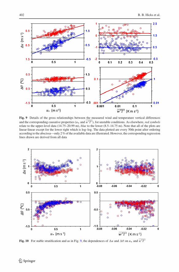
A first question concerns the strength of the physical cause-and-effect relationshipsbetween �u (and �θ ) and any of the variables included in conventional formulations. Fig-ure 9 addresses this question, presenting plots of the vertical finite differences �u (e.g.u20.99 − u14.75) and �θ versus u∗ and w′T ′ for the unstable case. It is seen that �θ is wellcorrelated with w′T ′(R = 0.83 and 0.85 for the higher and lower height intervals, respec-tively) but �u is not (R = 0.13 and 0.17). On the other hand, �u is well correlated with u∗(R = 0.84 and 0.85) whereas �θ is not (R = 0.31 and 0.27). The strength of the apparentrelationships is reassuring because it confirms much of the basis for the conventional rep-resentation of data in unstable stratification. The focus of micrometeorological research hastherefore appropriately been to relate the normalized wind gradient to properties known tobe influential—in this case the stability parameter Z/L .

Figure 10 extends the present considerations of linkages among causative variables to thestable case. An obvious conclusion from Fig. 10 is that there is no experimental basis (within

123


Fig. 9 Details of the gross relationships between the measured wind and temperature vertical differencesand the corresponding causative properties (u∗ andw′T ′), for unstable conditions. As elsewhere, red symbolsrelate to the upper-level data (14.75–20.99 m), blue to the lower (8.5–14.75 m). Note that all of the plots arelinear-linear except for the lower right which is log–log. The data plotted are every 50th point after orderingaccording to the abscissa—only 2 % of the available data are illustrated. However, the corresponding regressionlines drawn are derived from all data

Fig. 10 For stable stratification and as in Fig. 9, the dependences of �u and �θ on u∗ and w′T ′

123


Fig. 11 For conditions of stable stratification, the relationship between potential temperature differences andwind speed differences between levels about 6 m apart. The upper diagram is for the 14.75-m to 20.99-mheight interval, the lower for 8.5 m–14.75 m. The lines are drawn by eye to illustrate the appearance of twoseparate regimes that are more obvious in the lower levels

the present nighttime dataset made up of 15-min runs at a single location) for normalizing�uby u∗. These two quantities do not seem to be related. This generates uncertainty about thephysical relevance of the quantity φm and hence of the reasoning by which φm is considereda function of Z/L in stable conditions.

Nor is there an observational basis for including w′T ′ in the list of variables used toquantify�u in stable stratification. Note that these interpretations are not necessarily at oddswith conventional understanding, which relates to associations among averages and not to theindividual runs considered here. It should be remembered that the diagrams in Fig. 10 involvedata collected by two completely independent sensor systems—sonic anemometers for thevelocity differences and aspirated platinum resistance thermometers for the temperature dif-ferences. Figure 10 also shows no striking relationship between �θ and w′T ′, regardless ofthe strong expectations to the contrary.

Figure 11 extends consideration to the bulk differences alone. Notable in the two diagramsof Fig. 11 (especially in the case of the lower height interval) is the appearance of tworegimes, with one regime indicating a near-linear relationship between �θ and �u, and theother indicating near independence. Lines drawn by eye through the quasi-linear portions ofthe diagrams have the same slope—about 0.75 m s−1 difference per K difference—but it isclear that the relationship between�u and�θ cannot serve as the basis for a predictive tool,because the relationship is not single-valued.

123


7 Discussion and Conclusions

Most of the nighttime data considered here are influenced by a pervasive low-level jet (typ-ically at several hundred metres height, as has been well documented by Whiteman et al.(1997) for a site in nearby Oklahoma). This jet undoubtedly influences the wind field below it.It is thought that the present single-location 15-min averages do not address the full spectrumof transfer processes, there being a spatial component that is not captured. The three-pointrunning mean methodology adopted here was in response to this viewpoint. In this regard, itis of interest to note the summation by Panofsky et al. (1960)—“…theory and observationsagree well for near-neutral and unstable air; however, in stable air, factors not considered inthe similarity theory may become important.” They also mention that “The range of useful-ness of the log-linear wind profile is shown to be small,” a contention that is well supportedby the present finding, for stable conditions, of negligible dependence of vertical wind-speedgradients on u∗.

Scrutiny of the figures presented here shows that the transition between positive andnegative stability regimes is highly susceptible to the randomness generated by the non-linearities of the processes involved, and presumably to the spatial intermittence of the variouscontributing processes (q.v., Brooks 1961). For all but a few of the “neutral” cases, thesituation is transitional and therefore in violation of the stationarity assumption that underpinsmost considerations of neutral runs.

The Ocotillo data appear to indicate that free convection starts to influence near-surfacemicrometeorology soon after sunrise. Once sufficient surface heating is achieved (corre-sponding to Z/L ≈ −0.03), deep convection commences and thereafter dominates thesensible heat exchange process. Thus, the predictions of free convection are supported bythe unstable observations made using the Ocotillo tower over a wide range of instabilities.The picture then develops of a moving atmospheric medium with free convection embeddedwithin, with drag imposed by the surface, and with mechanically generated turbulence thatin turn is somewhat affected by buoyancy and convective interruption.

It is sometimes suggested that free convection can occur only in calm or nearly calmconditions. The data analyzed here support the opposite (and more conventional) view—that free convection can occur whenever the fiction velocity can be disregarded as a factorinfluencing the heat flux/gradient relationship.

The present analysis is of data collected as 15-min runs. In a subsequent but shorter inten-sive period, an additional sonic anemometer and thermometer system was installed at 5.5-mheight, to gain more detail for investigating alternative methods of evaluating local gradientsfrom point measurements. In this subsequent experimental period, data were collected at 60-min intervals, thus permitting a test of the adequacy of the 15-min datasets used in the presentanalysis. Comparison of the results indicates no cause for concern regarding the adequacy ofthe run length used here. The major differences lie in the increased uncertainties associatedwith the averages of the 60-min dataset, occasioned by the reduced number of runs withineach grouping of observations.

The present analysis unabashedly revisits ground that has been explored in detail previ-ously, and brings to question the relationships that are currently viewed as “given.” This re-analysis has been occasioned by the availability of copious data from a tower in surroundingsthat are seen as more representative of the Southern Great Plains than as a micrometeoro-logical outdoor laboratory. If the present results are found to be widely applicable, then therepercussions could be considerable since many numerical models assume the applicabilityof the legacy flux–gradient relations over short time intervals, whereas (a) it is found here

123


that the averages are rarely accurate descriptions of specific situations, and (b) the validityof the legacy relations is questionable.

Acknowledgments Mention of specific instrumentation does not constitute an endorsement; other systemscould work as well if not better. The data used here were collected as a part of an investigation of the planetaryboundary layer in support of the wind energy program of Duke Power, Inc. As part of the NOAA/DukeCooperative Research and Development Agreement, NOAA/ARL/ATDD and Duke Energy established aresearch station at Duke’s West Texas Ocotillo Wind Farm. The collaboration is with the Air ResourcesLaboratory of NOAA.

References

Baas P, Steeneveld GJ, van de Wiel BJH, Holtslag AAM (2006) Exploring self-correlation in flux–gradientrelationships for stably stratified conditions. J Atmos Sci 63:3045–3054

Brooks FA (1961) Need for measuring horizontal gradients in determining vertical eddy transfers of heat andmoisture. J Meteorol 18:589–596

Businger JA (1988) A note on the Businger–Dyer profiles. Boundary-Layer Meteorol 42:145–151Businger JA, Wyngaard JC, Izumi Y, Bradley EF (1971) Flux profile relationships in the atmospheric surface

layer. J Atmos Sci 28:181–189Dyer AJ (1974) A review of flux–profile relationships. Boundary-Layer Meteorol 7:363–372Dyer AJ, Hicks BB (1970) Flux–gradient relationships in the constant flux layer. Q J R Meteorol Soc 96:715–

721Garratt JR (1992) The atmospheric boundary layer. Cambridge University Press, UK, 316 ppGarratt JR, Hicks BB (1973) Momentum, heat and water vapour transfer to and from natural and artificial

surfaces. Q J R Meteorol Soc 99:680–687Hicks BB (1978) Some limitations of dimensional analysis and power laws. Boundary-Layer Meteorol

14:1451–1458Hicks BB (1981) An examination of turbulence statistics in the surface boundary layer. Boundary-Layer

Meteorol 21:389–402Klipp CL, Mahrt L (2004) Flux–gradient relationship, self-correlation and intermittency in the stable boundary

layer. Q J R Meteorol Soc 130:2087–2103Kochendorfer J, Meyers TP, Frank J, Massman WJ, Heuer MW (2012) How well can we measure the vertical

wind speed? Implications for fluxes of energy and mass. Boundary-Layer Meteorol 145:383–398Mahrt L (2010) Variability and maintenance of turbulence in the very stable boundary layer. Boundary-Layer

Meteorol 135:1–18Monin AS, Obukhov AM (1954) Basic relationships of turbulent mixing in the surface layer of the atmosphere.

Acad Nauk SSSR Trud Geofys Inst 24:163–187Panofsky HA, Blackadar AK, McVehil GE (1960) The diabatic wind profile. Q J R Meteorol Soc 86:390–398Plate EJ (1971) Aerodynamic characteristics of atmospheric boundary layers. US Atomic Energy Commission,

Springfield, VA, TID-25465, 190 ppPriestley CHB (1955) Free and forced convection in the atmosphere near the ground. Q J R Meteorol Soc

81:139–143Priestley CHB (1959) Turbulent transfer in the lower atmosphere. University of Chicago Press, Chicago,

130 ppWebb EK (1965) Aerial microclimate. Meteorol Monogr 6:27–58White R, Vogel CA, Pendergrass WR (2014) Flux Observations Ocotillo Texas (FOOT) Experiment. NOAA

Atmospheric Turbulence and Diffusion Division Technical Memorandum (in press)Whiteman CD, Bian X, Zhong S (1997) Low-level jet climatology from enhanced rawinsonde observations

at a site in the southern Great Plains. J Appl Meteorol 36:1363–1376

123

on the micrometeorology of the southern great plains 1: legacy relationships revisited

Documents