on the microeconomic theory of investment … theory of investment und… · *this paper is not a...

Chapter 13

ON THE M I C R O E C O N O M I C UNDER UNCERTAINTY*

ROBERT C. MERTON

Massachusetts Institute of Technology

T HEORY OF INVESTMENT

1. Introduct ion

Investment theory is the study of the individual behavior of households and economic organizations in the allocation of their resources to the available investment opportunities. For the purposes of investment theory, economic organizations are characterized as being members of one of two groups: "business firms" that hold as assets the physical means of production for the economy and finance their production decisions by issuing financial claims or securities; and "financial intermediaries" that hold financial claims as assets and finance these assets by issuing securities. Individuals or households are assumed to invest primarily in securities, and therefore invest only indirectly in physical assets. The markets in which these securities are traded are called the capital markets.

The natural starting point for the development of investment theory is to derive the investment behavior of individuals. It is traditional in economic theory to take the existence of households and their tastes as exogenous to the theory. However, this tradition does not extend to economic organizations and institutions. They are regarded as existing primarily because of the functions they serve instead of functioning primarily because they exist. Economic organizations are endogenous to the theory. To derive the functions of these economic organizations, therefore, the investment behavior of individuals must be derived first.

It is convenient to break the investment decision by individuals into two parts: (1) the "consumption-saving" choice where the individual decides how much of his

*This paper is not a survey of the economics and finance literature on investment theory which is already copious and whose rate of expansion has in recent years accelerated. Rather, the paper is designed to be a self-contained, but cryptic, introduction to some of the major problems in investment theory. In many cases, I have referenced excellent survey articles which themselves contain extensive bibliographies rather than attempt to reference all the important individual contributions to the subject. I gratefully acknowledge financial support from the National Science Foundation for this paper, and thank J. Cox and M. Latham for their helpful comments.

Handbook o f Mathematical Economics, voL 11, edited by K.J. Arrow and M.D. lntriligator North-Holland Publishing Company, 1982

602 R. C. Merton

wealth to allocate to current consumption and how much to invest for future consumption; and (2) the "portfolio selection" choice where he decides how to allocate his savings among the available investment opportunities. In general, the two decisions cannot be made independently. However, the format of the paper is to, first, solve the portfolio selection problem taking individual's consumption decisions and firms' production decisions as given, and to derive necessary conditions for financial equilibrium. Second, using these necessary conditions, the optimal production decision rules for firms are derived. Finally, the combined consumption and portfolio selection problem for individuals is solved.

It is, of course, not possible in a single paper to cover all the topics important to investment theory. However, two topics not covered here warrant special mention. First, while some necessary conditions for equilibrium are derived, I have not at tempted to integrate these conditions into a general equilibrium theory for the economy. Second, no at tempt has been made to make explicit how individuals and firms acquire the information needed to make their decisions, and in particular how they modify their behavior in environments where there are significant differences in the information available to various participants.

2. One-period portfolio selection

The basic investment choice problem for an individual is to determine the optimal allocation ol' his wealth among the available investment opportunities. The solution to the general problem of choosing the best investment mix is called portfolio selection theory. I begin the study of portfolio selection theory with its classic one-period formulation.

There are n different investment opportunities called securities and the random variable one-period return per dollar on security j is denoted by Zj ( j = 1 . . . . , n) where a "dollar" is the "unit of account". Any linear combination of these securities which has a positive market value is called a portfolio. It is assumed that the investor chooses at the beginning of a period that feasible portfolio allocation which maximizes the expected value of a v o n Neumann-Morgens te rn utility function 2 for end-of-period wealth. I denote this utility function by U(W), where

IAn important issue within this topic is the "information efficiency" of the stock market as derived in Fama (1965, 1970a) and Samuelson (1965, 1973). Grossman (1976) and Grossman and Stiglitz (1976) provide some additional insights. Hirshleifer (1973) has shown that, in the absence of production, private sector expenditures on information gathering may be "socially wasteful". More- over, ~ignificant further advances in general equilibrium theory will require explicit recognition of information production and its dissemination, and the development of such an integrated theory is just at its beginning.

2von Neumann and Morgenstem (1947). For an axiomatic description, see Herstein and Milnor (1953). Although the original axioms require that U be bounded, the continuity axiom can be extended to allow for unbounded functions. See Samuelson (1977) for a discussion of this and the St. Petersburg Paradox.

Ch. 13: Microeconomic Theory of Investment 603

W is the end-of-period value of the investor's wealth measured in dollars. It is further assumed that U is an increasing strictly concave function on the range of feasible values for W and that U is twice-continuously differentiable. 3 Because the criterion function for choice depends only on the distribution of end-of-period wealth, the only information about the securities that is relevant to the investor's decision is his subjective joint probability distribution for (Z 1 . . . . , Z n).

In addition, it is assumed that:

Assumption 1 ("Frictionless" markets)

There are no transactions costs or taxes, and all securities are perfectly divisible.

Assumption 2 ("Price taker")

The investor believes that his actions cannot affect the probability distribution of returns on the available securities. Hence, if w/is the fraction of the investor's initial wealth, W0, allocated to security j , then (w~ . . . . . wn) uniquely determines the probability distribution of his terminal wealth.

A riskless security is defined to be a security or feasible portfolio of securities whose return per dollar over the period is known with certainty.

Assumption 3 ("No-arbitrage opportunities")

All riskless securities must have the same return per dollar. This common return will be 'denoted by R.

Assumption 4 ("No-institutional" restrictions)

Short-sales of all securities, with full use of proceeds, is allowed without restriction. If there exists a riskless security, then the borrowing rate equals the lending rate. 4

Hence, the only restriction on the choice for the {wj} is the budget constraint that Y~nwj = 1.

Given these assumptions, the portfolio selection problem can be formally stated as

max E U ~.w/Z/Wo , (2.1) { wl ..... wn} 1

3The strict concavity assumption implies that investors are everywhere risk averse. While strictly convex or linear utility functions on the entire range imply behavior that is grossly at variance with observed behavior, the strict concavity assumption also rules out Friedman-Savage type utility functions whose behavioral implications are reasonable. The strict concavity also implies U ' (W)>0 which rules out individual satiation.

4The "borrowing rate" is the rate on riskless-in-terms-of-default loans. While virtually every individual loan involves some chance of default, the empirical "spread" in the rate on margin loans to individuals suggests that this assumption is not a "bad approximation" for portfolio selection analysis. An explicit analysis of risky loan evaluation is provided in Section 7.

604 R. C. Merton

subject to ~]~wj = 1, where E is the expecta t ion opera to r for the subjective jo in t p robabi l i ty distribution. I f (w~' . . . . . w*) is a solution to (2.1), then it will satisfy the first-order condit ions

E{U'(Z*Wo)Zj}=X, j = 1 ,2 , . . . , n, (2.2)

where the pr ime denotes derivative; Z * - Y,~wTZ j is the r a n d o m variable re turn per dollar on the opt imal portfol io; and X is the Lagrange mult ipl ier for the budget constraint . Together with the concavi ty assumpt ions on U, if the n × n va r i ance -cova r i ance matr ix of the returns (Z~ . . . . . Zn) is nonsingular and an interior solution exists, then the solution is unique. 5 This non-singular i ty condi- t ion on the returns distr ibution el iminates " r e d u n d a n t " securities (i.e. securities whose returns can be expressed as exact l inear combina t ions of the returns on other available securities). 6 It also rules out that any one of the securities is a riskless security.

I f a riskless security is added to the menu of available securities (call it the ( n + l ) s t security), then it is the convent ion to express (2.1) as the following uncons t ra ined maximiza t ion problem:

max E U ( Z j - R ) + R W o , (2.3) {W 1 . . . . . Wn} j

where the por t fol io allocations to the risky securities are uncons t ra ined because the fract ion allocated to the riskless security can always be chosen t o satisfy the budget constraint (i.e. w*+l = 1 - ] ~ wT). The f irst-order condi t ions can be wri t ten as

E { U ' ( Z * W o ) ( Z j - R ) } = O , j = l , 2 . . . . . n , (2.4)

n where Z* can be rewrit ten as ~,1 wj ( Z j - R ) + R . Again, if it is assumed that the va r i ance -cova r i ance matr ix of the returns on the r isky securities is non-s ingular and an interior solution exists, then the solution is unique.

SThe existence of an interior solution is assumed throughout the analyses in this paper. For a complete discussion of the necessary and sufficient conditions for the existence of an interior solution, see Lelsand (1972) and Bertsekas (1974).

6For a trivial example, shares of General Motors with odd serial numbers are technically different from shares of GM with even serial numbers, and are, therefore, technically different securities. However, because their returns are identical, they are perfect substitutes from the point of view of investors. In portfolio theory, securities are operationally defined by their return distributions, and therefore two securities with identical returns are indistinguishable.


In both (2.1) and (2.3), no explicit consideration has been given for the treatment of bankruptcy (i.e. Z * < 0 ) . To rule out bankruptcy, the additional constraint that the probability of Z * ) 0 be one could be imposed on the choices for (w~,...,w~*). 7 If the reason for this constraint is to reflect institutional restrictions designed to avoid individual bankruptcy, then it is too weak because the probability assessments on the (Zj} are subjective. A more realistic treatment would be to forbid borrowing and short-selling in conjunction with limited-liability securities where, by law, Zj/> 0. These rules can be formalized as restrictions on the allowable set of {N} such that w 7 ~>0, j= 1,2 . . . . , n + 1, and (2.1) or (2,3) can be solved using the methods of Kuhn and Tucker 8 for inequality constraints. However, since the creation of limited-liability securities is itself a bankruptcy rule and only one of many that might be proposed, such explicit restrictions will not be imposed. Rather, it is simply assumed that there exists a bankruptcy law which allows for U ( W ) to be defined for W < 0 and that this law is consistent with the continuity and concavity assumptions on U.

The optimal demand functions for risky securities, {wj*W0}, and the resulting probability distribution for the optimal portfolio will, of course, depend on the risk preferences of the investor, his initial wealth, and the joint distribution for the securities' returns. It is well known that the von Neumann-Morgens te rn utility function can only be determined up to a positive affine transformation. Hence, the preference orderings of all choices available to the investor are completely spedfied by the P ra t t -Ar row 9 absolute risk-aversion function which can be written as

-v"(w) A(W)=- U'(W) ' (2.5)

and the change in absolute risk aversion with respect to a change in wealth is, therefore, given by

V'"(W)V,,(W) ]" (2.6)

7If U is such that U'(0)= oo, and by extension, U'(W) = ~, W<0, then from (2.2) or (2.4), it is easy to show that the probability of Z*~<0 is a set of measure zero.

8Kuhn and Tucker (1951). The analysis of the "no short-sales" case is complicated and leads to virtually no theorems. Although in actual markets there are some restrictions on short sales, these restrictions may not be too important because limited liability securities (e.g. put options) can and have been created that provide essentially the same type of return as a short sale.

9The behavior associated with the utility function V(W)-~aU(W) + b, a>0, is indistinguishable from the behavior associated with U(W). Note: A(W) is invariant to any positive affine transformation of U(W). See Pratt (1964).

606 R. C. Merton

By the assumption that U(W) is increasing and strictly concave, A(W) is positive, and such investors are called risk-averse. An alternative, but related, measure of risk aversion is the relative risk-aversion function defined to be

v"(w)w 6-fl (w)= u'(w) =A(W)W, (2.7)

and its change with respect to a change in wealth is given by

~ ' ( W ) = A ' ( W ) W + A ( W ) . (2.8)

The certainty equivalent end-of-period wealth, W~, associated with a given portfolio for end-of-period wealth whose random variable value is denoted by W, is defined to be that value such that

(2.9)

i.e. W~ is the amount of money such that the investor is indifferent between having this amount of money for certain or the portfolio with random variable outcome W. The term "risk-averse" as applied to investors with concave utility functions is descriptive in the sense that the certainty equivalent end-of-period wealth is always less than the expected value of the associated portfolio, E{W}, for all such investors. The proof follows directly by Jensen's Inequality: if U is strictly concave, then

U(W ) } <U(E{ W } )

whenever W has positive dispersion, and, because U is a non-decreasing function of w, <E{W}.

The certainty-equivalent can be used to compare the risk-aversions of two investors. An investor is said to be more risk averse than a second investor if for every portfolio, the certainty-equivalent end-of-period wealth for the first investor is less than or equal to the certainty equivalent end-of-period wealth associated with the same portfolio for the second investor with strict inequality holding for at least one portfolio.

While the certainty equivalent provides a natural definition for comparing risk aversions across investors, Rothschild and Stiglitz 1° have attempted in a corresponding fashion to define the meaning of "increasing risk" for a security so that

l°Rothschild and Stiglitz (1970, 1971). There is an extensive literature, not discussed here, that uses this type of risk measure to determine when one portfolio "stochastically dominates" another. Cf. Hadar and Russell (1970, 1971), Hanoch and Levy (1969), and Bawa (1975).

Ch. I3: Microeconomic Theory of Investment 607

the "riskiness" of two securities or portfolios can be compared. In comparing two portfolios with the same expected values, the first portfolio with random variable outcome denoted by W l is said to be less risky than the second portfolio with random variable outcome denoted by W 2 if

E( U(W1) }>~E( U(W2) } (2.1o)

for all concave U with strict inequality holding for some concave U. They bolster their argument for this definition by showing its equivalence to the following two other definitions:

There exists a random variable Z such that W 2 has the same distribution as W l + Z where the conditional expectation of Z given the outcome on W 1 is zero (i.e. W 2 is equal in distribution to W l plus some "noise").

(2.11)

If the points of F and G, the distribution functions of W 1 and W 2 are confined to the closed interval [a, b], and T(y)~ fY[G(x)-F(x)]dx, then T(y)>O and T ( b ) = 0 (i.e. W 2 has more "weight in its tails" than w~).

(2.12)

A feasible portfolio with return per dollar Z will be called an efficient portfolio if there exists an increasing, strictly concave function V such that E(V'(Z)(Zj-R)}=0, j = 1,2,. . . , n. Using the Rothschild-Stiglitz definition of "less risky", a feasible portfolio will be an efficient portfolio only if there does not exist another feasible portfolio which is less risky than it is. All portfolios that are not efficient are called inefficient portfolios.

Proposition 2.1

If the set of available securities contain no redundant securities, then no two efficient portfolios have the same risk in the Rothschild-Stiglitz sense.

Proof Let Z~ and Z [ denote the random variable returns per dollar on two distinct efficient portfolios. Let E denote the expectation operator over their joint distribution. The proof goes by contradiction. If the two portfolios have the same risk, then E ( Z ~ ) = E ( Z 2) and E{U(Z~)}=E{U(Z2e)} for every concave U. Con- sider the following artificial security with return per dollar Z given by Z = YZ~e + (1 - Y)Z 2, where Y= 1 with probability 8 ( 0 < 8 < 1) and Y =0 with probability (1 -8 ) and Yis independent of Z 1 and Z 2. It follows that Ez(Z)=E(Z~)=E(Z~)

608 R. C. Merton

and Ez(U(Z)}=3EfU(Z~)}+(1-3)EfU(Z2))=EfU(Z~e)}=EfU(Z~)}, i.e. Z has the same risk as either Z 1 or Z 2. Define Z~ --Ey(Z)=3Z ~ + ( 1 - 3 ) Z 2. By the independence of Y and Jensen's Inequality, E(U(Z~)}~Ez(U(Z)} with equality holding if and only if Z=Z~ because U can be taken to be strictly concave. If the inequality holds, then Z~ is less risky than Z because E ( Z ~ ) = E z ( Z ). But Z~ is the random variable return on a feasible portfolio gotten by combining the two portfolios Z~ and Z~ with portfolio weights [3,(1-3)] . Hence, Z 8 is less risky than both Ze ~ and Z d. But this contradicts the hypothesis that these portfolios are efficient. Hence, Z=Z~, and this is possible if and only if Z~ = Z 2. If there are no redundant securities, then Z~ = Z 2 if and only if the two portfolios contain identical holdings, but this contradicts the hypothesis that the two portfolios are distinct.

Hence, from the definition of an efficient portfolio and Proposition 2.1, it follows that no two portfolios in the efficient set can be ordered with respect to one another. From (2.10), it follows immediately that every effident portfolio is a possible optimal portfolio, i.e. for each efficient portfolio there exists an increasing, concave U and an initial wealth W 0 such that the efficient portfolio is a solution to (2.1) or (2.3). Furthermore, from (2.10), all risk-averse investors will be indifferent between selecting their optimal portfolios from the set of all feasible portfolios or from the set of efficient portfolios. Hence, without loss of generality, I will assume that all optimal portfolios are efficient portfolios.

With thes6 general definitions established, I now turn to the analysis of the optimal demand functions for risky assets and their implications for the distributional characteristics of the underlying securities. A note on notation: the symbol Z e will be used to denote the random variable return per dollar on an efficient portfolio, and a bar over a random variable (e.g. Z) will denote the expected value of that random variable.

Theorem 2.1

If Z denotes the random variable return per dollar on any feasible portfolio and if (Z e - Z e) is riskier than ( Z - Z) in the Rothschild and Stiglitz sense, then Z~ > Z

Proof

By hypothesis, E{U([Z--Z]Wo)}>E{U([Z e --Ze]W0) }. If Z>~Z~, then trivially, E(U(ZWo)}>E(U(Z~Wo) }. But Z is a feasible portfolio and Ze is an efficient portfolio. Hence, by contradiction, Z e > Z

Corollary 2.1.a

If there exists a riskless security with return R, then Z~ ~>R with equality holding only if Z~ is a riskless security.


Proof

The riskless security is a feasible portfolio with expected return R_ If Z~ is risktess, then by Assumption 3, Z e =R . If Z e is not riskless, then (Z~ - Z e ) is riskier than ( R - R ) . Therefore, by Theorem 2.1, Z~ >R.

Theorem 2.2

The optimal portfolio for a non-satiated, risk-averse investor will be the riskless security (i.e. w*+t = 1, 9" = 0 , j = 1,2 . . . . . n) if and only if ~ = R for j = 1,2 . . . . , n.

Proof

From (2.4), {w? . . . . . w*} will satisfy E ( U ' ( Z * W o ) ( Z j - R ) } = O , j = l , 2 . . . . . n. If =R, j-= 1,2,. . . , n, then Z * = R will satisfy these first-order conditions. By the

strict concavity of U and the non-singularity of the variance-covariance matrix of returns, this solution is unique. This proves the "if" part. If Z* = R is an optimal solution, then we can rewrite (2.4) as U'(RWo)E(Z j - R ) = 0 . By the non-satiation assumption, U'(RWo)>O. Therefore, for Z * = R to be an optimal solution,

= R , j = 1,2 . . . . . n. This proves the "only if" part.

Hence, form Corollary 2.1.a and Theorem 2.2, if a risk-averse investor chooses a risky portfolio, then the expected return on that portfolio exceeds the riskless rate, and a risk-averse investor will choose a risky portfolio if, at least, one available security has an expected return different from the riskless rate.

Define the notation E(Y[ X 1 . . . . . Xq) to mean the conditional expectation of the random variable Y, conditional on knowing the realizations for the random variables ( X 1 . . . . . Xq).

Theorem 2.3

If there exists a feasible portfolio with return Zp such that for security s, Zs = Z p + e,, where E( e , )= E( es l Zp, Zj, j = 1,..., n, j=/= s )=O, then the fraction of every efficient portfolio allocated to security s is the same and equal to zero.

Proof

The proof follows by contradiction. Let Z e be the return on an efficient portfolio with fraction 6 s ~ 0 allocated to security s. Let Z be the return on a portfolio with the same fractional holdings as Z e except instead of security s, it holds the fraction 6s in feasible portfolio Zp. Hence, Z e = Z - ~ - r s ( Z s --Zp) or Z e = Z +6,e~. By hypothesis, Ze = Z and by construction, E(e~ [ Z ) = 0. Therefore, for 6, v ~ 0, Z~ is riskier than Z in the Rothschild-Stiglitz sense. But this contradicts the hypothesis that Z e is an efficient portfolio. Hence, 6, = 0 for every efficient portfolio.

610 R. C. Merton

Corollary 2.3. a

Let q~ denote the set of n securities with returns (Z l . . . . , Zs_ l, Z s, Zs+l , . . . , Zn) and q/ denote the same set of securities except Zs is replaced with Zs,. If Z s ,=Zs +e s and E(e~)=E(eslZ 1 . . . . . Z~_I, Z~, Z~+ 1 . . . . . Zn)=0, then all risk- averse investors would prefer to choose their optimal portfolios from + rather than +'.

The proof is essentially the same as the proof of Theorem 2.3 with Z~ replacing Zp. Unless the holdings of Z~ in every efficient portfolio are zero, ~b will be strictly preferred to +'.

Theorem 2.3 and its corollary demonstrate that all risk-averse investors would prefer any "unnecessary" uncertainty or "noise" to be eliminated. In particular, by this theorem the existence of lotteries is shown to be inconsistent with strict risk aversion on the part of all investors) 1 While the inconsistency of strict risk aversion with observed behavior such as betting on the numbers can be "explained" by treating lotteries as consumption goods, it is difficult to use this argument to explain other implicit lotteries such as callable, sinking fund bonds where the bonds to be redeemed are selected at random.

As illustrated by the partitioning of the feasible portfolio set in to its efficient and inefficient parts and the derived theorems, the Rothschild-Stiglitz definition of increasing risk is quite useful for studying the properties of optimal portfolios. However, it is important to emphasize that these theorems apply only to efficient portfolios and not to individual securities or inefficient portfolios. For example, if ( Z j - ~ ) is riskier than ( Z - Z ) in the Rothschild-Stiglitz sense and if security j is held in positive amounts in an efficient or o_ptimal portfolio (i.e. wj* >0), then it does not follow that ~ must equal or exceed Z. In particular, if w 7 > 0, it does not follow that ~ must equal or exceed R. Hence, to know that one security is riskier than a second security using the Rothschild-Stiglitz definition of increasing risk provides no normative restrictions on holdings of either security in an efficient portfolio. And because this definition of riskier imposes no restrictions on the optimal demands, it cannot be used to derive properties of individual securities' return distributions from observing their relative holdings in an efficient portfolio. To derive these properties, a second definition of risk is required. However, discussion of this measure is delayed until Section 3.

In closing this section, comparative statics results are derived for the optimal risky security demand in the special case of a single risky security and a riskless security (i.e. n = 1). Additional results for the general case of many risky securities can be found in Fisher (1972).

I lI believe that Christian von Weizs~icker proved a similar theorem in unpubfished notes some years ago. However, I do not have a reference.

\,\ Ch. 13: Mic/Oeconomic Theory of Investmem 611

Define g by

x--=-E{ U " ( W * ) ( Z - R ) 2 W o } >0 , (2.13)

where Z is the random variable return per dollar on the single risky security and W*=[w*(Z-R)+R]Wo is the random variable end-of-period wealth for the optimal allocation.

Applying the Implicit Function Theorem to (2.4), the change in the proportion of the optimal portfolio allocated to the risky security with respect to a change in initial wealth can be written as

Ow* _ -E(w*a2~(W*)U'(W*)(W*-RWo) } OWo (w,wo)~ ' , for w*¢O,

= 0 for w* =0,

where ~ is the relative risk-aversion function defined in (2.7). If U is such that is a constant, then Ow*/OW o = 0 because E(U'(W*)(W*-RWo)}=O from (2.4). By integrating (2.7) twice, the general class of concave utility functions that exhibit constant relative risk aversion can be written as

v(w)=c [ w,-1] 1[ V J "~-C2' (2.15)

where Ct and C 2 are any constants such that C t > 0 and y < 1. Because von Neumann-Morgenstern utility functions are unique only up to a positive affine transformation, all distinct members of this class are determined by the single parameter y. The relative risk-aversion function ~ equals (1 -~ , )>0 . Hence, for investors with utility functions in this class, a larger value of ~, implies a smaller value of relative risk aversion. Moreover, for all portfolios that can be ranked, Z2 it is straightforward to show that 0w*/0~{>0.

For each possible outcome for W*, we have by the Mean Value Theorem that there exists a number O=O(W*), 0~<0~< l, such that

~ ( w * ) = ~ (R Wo) + ~ ' ( , ) ( W * - R Wo), (2.16)

where ~=--RWo+O(W*-RWo) and ~ ' is defined in (2.8). Substituting from

~2Because the iso-elastic family is not well defined for W<0, portfolios with a positive probability of negative end-of-period wealth cannot be ranked.

612

(2.16) into (2.14) with w*v~0, (2.14) can be rewritten as

Ow* _ - E { w * ~ ' ( ~ I ) U ' ( W * ) ( W * - R W o ) 2 }

OWo ( w*Wo

R. C. Merton

(2.17)

From (2.17) a sufficient condition for the optimal proportion in the risky security to decline with an increase in initial wealth is that ~ 'w* >0. Similarly, a sufficient condition for the optimal proportion to increase is that ~ ' w * < 0 . Hence, for investors with strictly increasing (decreasing) relative risk aversion, an increase in initial wealth will induce a decrease (increase) in the absolute proportion of the optimal portfolio allocated to the risky security, I w*[.

From (2.14) the change in the dollar allocation to the risky security in the optimal portfolio with respect to a change in initial wealth can be written as

O(w*W o ) _ - - R E { w * A ( W * ) U ' ( W * ) ( W * - R W o ) } 0Wo (w . )2 , w* 0,

=0, w* =0, (2.18)

where A is the absolute risk-aversion function defined in (2.5). If U is such that A is a constants then ~(w*Wo) /~W o =0. By integrating (2.5) twice, the general class of concave utility functions that exhibit constant absolute risk aversion can be written as

U( W ) = C 2 - C,e -~,w, (2.19)

where C l and C 2 are any constants such that CI>0 and /~>0. All distinct members of this class are determined by the single parameter/~ which is equal to the absolute risk-aversion function, and O(w*W0)/3#<0.

Again, using the Mean Value Theorem, A(W*) can be written as

A(W*)=A( RWo)+A'(n)(W*-RWo). (2.20)

Substituting from (2.20) into (2.18) with w*=~ O, (2.18) can be rewritten as

O(w*Wo) _ - R E { w * A ' ( ~ I ) U ' ( W * ) ( W * - R W o ) 2 }

OWo (2.21)

From (2.21) a sufficient condition for the optimal dollar investment in the risky security to decline is that A'w* >0, and a sufficient condition for it to increase is

Ch. I3: Microeconomic Theory of Investment 613

that A'w* <0. Hence, for investors with strictly increasing (decreasing) absolute risk aversion, an increase in initial wealth will induce a decrease (increase) in the absolute dollar position in the risky security, I w*Wo [.

Although the direction of change in both the proportional and absolute dollar holdings of the risky security depends upon the sign of w*, the sign of w* is determined solely by the sign of (Z-R) . From Theorem 2.2, w* = 0 if and only if Z---R. If w*v~0, then Z*>R because an optimal portfolio is an efficient portfolio. But Z*=R+w*(Z-R). Hence, w*(Z--R)>O if w*v~0. Therefore, for any non-satiated, risk-averse investor, the sign of w* will equal the sign of (Z-R). Warning: this condition need not obtain with respect to an individual security when there is more than one risky security, i.e. the sign of w 7 need not equal the sign of ( ~ - R ) for n> 1.

From (2.14), the change in w* with respect to a change in the risky security's expected return Z can be written as

Ow* _ z{ u ' ( w * ) [ 1 - A ( w * ) ( w * - R Wo )] ) (2.22)

Inspection of (2.22) shows that the sign of Ow*/OZ is ambiguous. However, three sufficient conditions for Ow*/OZ to be positive are:

(i) w* =0;

o r

(ii) A ' (W)<0; (2.23)

o r

W (iii) ~ ( W ) _ < - W_RWo, for RW 0 < W~< W +,

where W + equals the maximum possible outcome for W*. Conditions (i) and (iii) follow directly from (2.22) and (ii) follows from the substitution for A(W*) from (2.20) into (2.22).

From (2.14) the change in w* with respect to a change in R can be written as

Ow* _ -E(U ' (W*)[ (w*)2+A(W*)w*(1- -w*) (W*--RWo)] ) (2.24)

OR

From (2.24), Ow*/OR can be either positive or negative. Two sufficient conditions

614 R. C. Merton

for Ow*/OR to be negative are:

(i) A'(W)>=O and w*(1-w*)>-_0

or

(ii) A'(W)<=O and w * ( 1 - w * ) < 0 .

(2.15)

These conditions follow from the substitution for A(W*) from (2.20) into (2.24). Rothschild and Stiglitz 13 have examined the effect on the optimal demand for

the risky security of an increase in that security's riskiness. As with the other comparative statics results derived here, they found that the change in the optimal demand can be either positive or negative. A sufficient condition for an increase in risk to decrease the demand for the risky security is that f (Z ) = (Z--R)U'([w*(Z--R)+R]Wo) be concave in Z. It is straightforward to show by differentiating f (Z ) twice with respect to Z that if relative risk aversion is less than or equal to R and non-decreasing and if absolute risk aversion is non- increasing, t h e n f ( Z ) is strictly concave for w* > 0 and strictly convex for w* <0.

In summary, even for the simplest case of one risky security and a riskless security, the sign of the change in the optimal demand for the risky security with respect to changes in its probability distribution is consistently ambiguous unless restrictions are placed on the class of utility functions or on the class of probability distributions for Z.

3. Risk measures for securities and portfolios in the one-period model

In the previous section the Rothschild-Stiglitz measure for the risk of a security was defined, and the comparative statics of an increase in a security's risk was analyzed in the special case of a single risky security and a riskless security. However, in the more-than-one risky security portfolio problem the Rothschild- Stiglitz measure is not a natural definition of risk for a security. In this section a second definition of increasing risk is introduced, and it is argued that this second measure is a more appropriate definition for the risk of a security. Although this second measure will not in general provide the same orderings as the Rothschild- Stiglitz measure, it is further argued that the two measures are not in conflict, and indeed, are complementary.

If Z e is the random variable return per dollar on an efficient portfolio with positive dispersion, then let V(Z e) denote an increasing, strictly concave function

J3Rothschild and Stiglitz (1971, pp. 70-74).

Ch. 13." Microeconomic Theory of Investment 615

such that

E{V'(Ze)(Zj--R))=O, j = l , 2 . . . . . n,

i.e. V is a concave utility function such that an investor with initial wealth W 0 = 1 and these preferences would select this efficient portfolio as his optimal portfolio. While such a function V will always exist, it will not be unique. If cov[x~, x2] is the functional notation for the covariance between the random variables x~ and x 2, then define the random variable, Y(Ze), by

V'(Ze)-E(V'(Ze)) (3.1)

Y(Ze) is well defined as long as Z~ has positive dispersion because cov[V'(Ze), Ze] <0.14 It is understood that in the following discussion "efficient portfolio" will mean "efficient portfolio with positive dispersion". Let Zp denote the random variable return per dollar on any feasible portfolio p.

Definition

The measure of risk of portfolio p relative to efficient portfolio K with random variable return Z~, b~, is defined by

Zp] and portfolio p is said to be riskier than portfolio p' relative to efficient portfolio K if h K > h K -p -p' .

Theorem 3.1

If Zp is the return on a feasible portfolio p and Zff is the return on efficient portfolio K, then Zp - R = bpr( Z~ - R).

Proof

From the definition of V(Zf ) , E ( V ' ( Z ~ ) ( Z j - R ) } = 0 , j = 1,2,. . . ,n. Let $j be the fraction of portfofio p allocated to security j. Then, Z e = ~ j ( Z j - R) + R, and ~$ jE(V ' (Ze ) (Z j -R ) )=E(V ' (Ze ) (Zp -R) }=O. by a similar argument, E{V'(Zf)(Ze x - R)) =0. Hence, cov[V'(Zf), Z f ] = ( R - Z~)E{V ' (Z f ) } and cov[V'(Zff), Zp]-=(R - Zp)E{V'(Z~K)). By Corollary 2.1.a, Z f f > R. Therefore, covtr(z , z p l - - ( R - -

"4For a proof, see Theorem 236 in Hardy, Littlewood, and Prlya (1959).

616 R. C. Merton

Hence, the expected excess return on portfolio p, Zp--R, is in direct proportion to its risk, and because Z f > R , the larger is its risk, the larger is its expected return. Thus, Theorem 3.1 provides the first argument why bp x is a natural measure of risk. for individual securities.

A second argument goes as follows. Consider an investor with utility function U and initial wealth W 0 who solves the portfolio selection problem

maxE( U([wZ. + (1-w)Z]Wo ) ), w L \ L J

where Z is the return on a portfolio of securities and Zj is the return on the securityj. The optimal mix, w*, will satisfy the first-order condition

E(U'([w% + (1-w*)Z] Wo)(Zj-Z))=0. (3.2)

If the original portfolio of securities chosen was this investor's optimal portfolio (i.e. Z=Z*) , then the solution to (3.2) is w* =0. However, an optimal portfolio is an efficient portfolio. Therefore, by Theorem 3.1, ~ - R = bj*(Z* - R). Hence, the "risk-return tradeoff" provided in Theorem 3.1 is a condition for personal portfolio equilibrium. Indeed, because securityj may be contained in the optimal portfolio, w*W 0 is similar to an excess demand function, b 7 measures the contribution of security j to the Rothschild-Stiglitz risk of the optimal portfolio in the sense that the investor is just indifferent to a marginal change in the holdings of security j provided that ~-R=bT(Z*--R ). Moreover, by the Implicit Function Theorem, we have from (3.2) that

Ow* _ w'WoE (u"(z-z j ) )-E(U') E(U"(z-zj) 2)

>0, atw*=O. (3.3)

Therefore, if ~ lies above the "risk-return" line in the (Z-b*)_plane, then the investor would prefer to increase his holdings in security j, and if Zs lies below the line, then he would prefer to reduce his holdings. If the risk of a security increases, then the risk-averse investor must be "compensated" by a corresponding increase in that security's expected return if his current holdings are to remain unchanged.

The Rothschild-Stiglitz measure of risk is clearly different from the bf measure here. The Rothschild-Stiglitz measure provides only for a partial ordering while the bf measure provides a complete ordering. Moreover, they can give different rankings. For example, suppose the return on security j is independent of the return on efficient portfolio K, then bf =0 and ~ =R. Trivially, b x =0

Ch. 13. Microeconomic Theory of Investment 617

for the riskless security. Therefore, by the bf measure, security j and the riskless security have equal risk. However, if security j is not riskless, then by the Rothschild-Stiglitz measure security j is more risky than the riskless security. Despite this, the two measures are not in conflict and, indeed, are complementary. The Rothschild-Stiglitz definition measures the "total risk" of a security in the sense that it compares the expected utility from holding a security alone with the expected utility from holding another security alone. Hence, it is the appropriate definition for identifying optimal portfolios and determining the efficient portfolio set. However, it is not useful for defining the risk of securities generally because it does not take into account that investors can mix securities together to form portfolios. The bf measure does take this into account because it measures the only part of an individual security's risk which is relevant to an investor: namely, the part that contributes to the total risk of his optimal portfolio. In contrast to the Rothschild-Stiglitz measure of total risk, the bf measures the "systematic risk" of a security (relative to efficient portfolio K). Of course, to determine the b F the efficient portfolio set must be determined. Because the Rothschild-Stiglitz measure does just that, the two measures are complementary.

Other properties of the bff measure of systematic risk are:

Property 1

If a feasible portfolio p has portfolio weights (81, 6 2 . . . . . ~n), then b~=Y~3jbf. The systematic risk of a portfolio is the weighted sum of the systematic risks of its component securities.

Property 1 follows directly from the linearity of the covariance operator, cov[xl, x2], with respect to the random variable x 2.

Let p and p' denote any two feasible portfolios and let K and L denote any two efficient portfolios.

Property 2

If be ~ = 0 for some efficient portfolio K, then bp c = 0 for any efficient portfolio L.

Property 2 follows from Theorem 3.1 and Corollary 2.1.a. If b x =0, then @ = R because Ze K > R. But if ~ = R and Ze r > R, then bp c =0.

Property 3 > 2>

b, if and only if b,

Property 3 follows from Property 2 if bp K = b~ = 0. Suppose bff v ~ 0, then Property 3 follows from Theorem 3.1 because

618 R. C. Merton

Property 3 provides a third argument why @: is a natural measure of risk for individual securities, namely the ordering of securities by their systematic risk relative to a given efficient portfolio will be identical to their ordering relative to any other efficient portfolio. Hence, given the set of available securities, there is an unambiguous meaning to the statement "security j is riskier than security i ".

Property 4

If portfolio p is an efficient portfolio (call it the Kth one with Zp = Z~X), then for any efficient portfolio L, @ > 0 and in particular, bff = 1. Hence, all efficient portfolios have positive systematic risk relative to any efficient portfolio.

Property 4 follows from Theorem (3.1) and Corollary 2.1.a.

Property 5

If the systematic risk of portfolio p is defined by its expected return_ Zp, and if portfolio p is said to be riskier than portfolio p' if and only if Zp > Zp,, then this measure of systematic risk is equivalent to the b~ measure.

Property 5 follows directly from Theorem (3.1), Corollary 2.1.a, and Property 3. Although the expected return of a security provides an equivalent ranking to its

bff measure, the bp K measure is not vacuous. There exist non-trivial information sets which allow )5; to be determined without knowledge of Zp. For example, consider a model in which all investors agree on the joint distribution of the returns on securities. Suppose we know the probability distribution of the optimal portfolio, Z*Wo, and the utility function U for some investor. From (3.1) we therefore know the distribution of Y(Z*). For security j, define the random variable ej = Z j - Z / . Suppose, furthermore, that we have enough information about the joint distribution of Y(Z*) and e/ to compute cov[Y(Z*), ej], but do not know ~.15 By the definition of covariance, cov[Y(Z*), ej]=cov[Y(Z*), Zj]=b 7. However, Theorem 3.1 is a necessary condition for equilibrium in the securities market. Hence, we can deduce the equilibrium expected return on securityj from

= R + b T ( Z * - R ) . An analysis of the necessary information sets required to deduce the equilibrium structure of security returns is an important part of portfolio theory, and further discussion of this topic is provided in Sections 4 and 5.

15A sufficient amount of information would be the joint distribution of Z* and ej. The necessary amount of information will depend upon_the functional form of U'. However, in no case will a necessary condition be knowledge of Zj.


4. Spanning, separation, and mutual fund theorems

Definition

A set of M feasible portfolios with random variable returns (X 1 . . . . , X~t ) are said to span the space of portfolios contained in set xt' if and only if for any portfolio in 't, with return denoted by Zp, there exists numbers (61 . . . . . 6~4), ~ 6 j = 1, such that Z p = ~ S j X j . If N is the number of securities available to generate the portfolios in ,I, and if M* denotes the smallest number of feasible portfolios that span the space of portfolios contained in q', then M* <_--N.

As was illustrated in Section 2, very little can be derived about the structure of optimal portfolio demand functions unless further restrictions are imposed on the class of investors' utility functions or the class of probability distributions for securities' returns. A particularly fruitful set of such restrictions is the one that provides for a non-trivial (i.e. M * < N ) spanning of the feasible portfolio set. Indeed, the spanning property leads to a collection of "mutual fund" or "separation" theorems that are the core of modern financial theory.

A mutual fund is a financial intermediary that holds as its assets a portfolio of securities and issues as liabilities shares against these assets. Unlike the portfolio of an individual investor, the portfolio of securities held by a mutual fund need not be an efficient portfolio. The connection between mutual funds and the spanning property can be seen in the following theorem:

Theorem 4.1

If there exist M mutual funds whose portfolios span the portfolio set 'I', then all investors will be indifferent between selecting their optimal portfolios from ,t' or from portfolio combinations of just the M mutual funds.

The proof of the theorem follows directly from the definition of spanning. If Z* denotes the return on an optimal portfolio selected from 't t and if ~ denotes the return on the j t h mutual fund's portfolio, then there exist portfolio weights (~ ..... 6~t ) such that Z*=~,~67X j. Hence, any investor would be indifferent between the portfolio with return Z* and the (6*t, . . . , 3~) combination of the mutual fund shares.

Although the theorem states "indifference", if there are information-gathering or other transactions costs and if there are economies of scale, then investors would prefer the mutual funds whenever M<N. By a similar argument, one would expect that investors would prefer to have the smallest number of funds necessary to span 't'. Therefore, the smallest number of such funds, M*, is a particularly important spanning set. Hence, the spanning property can be used to derive an endogenous theory for the existence of financial intermediaries with the

620 R.C. Merton

functional characteristics of a mutual fund. Moreover, from these functional characteristics a theory for their optimal management can be derived.

For the mutual fund theorems to have serious empirical content, the minimum number of funds required for spanning M* must be significantly smaller than the number of available securities, N. When such spanning obtains, the investor's portfolio selection problem can be separated into two steps: first, individual securities are mixed together to form the M* mutual funds; second, the investor allocates his wealth among the M* funds' shares. If the investor knows that the funds span the space of optimal portfolios, then he need only know the joint distribution of (X1,..., XM.) to determine his optimal portfolio. It is for this reason that the mutual fund theorems are also called "separation" theorems. However, if the M* funds can be constructed only if the fund managers know the preferences, endowments, and probability beliefs of each investor, then the formal separation property will have little operational significance.

In addition to providing an endogenous theory for mutual funds, the existence of a non-trivial spanning set can be used to deduce equilibrium properties of individual securities' returns and to derive optimal decision rules for business firms making physical investments. Moreover, in virtually every model of portfolio selection in which empirical implications beyond those presented in Sections 2 and 3 are derived, some non-trivial form of the spanning property obtains.

While the determination of conditions under which non-trivial spanning will obtain is, in a broad sense, a subset of the traditional economic theory of aggregation, the first rigorous contributions in portfolio theory were made by Arrow (1964), Markowitz (1959), and Tobin (1958). In each of these papers, and most subsequent papers, the spanning property is derived as an implication of the specific model examined, and therefore such derivations provide 0nly sufficient conditions. In two notable exceptions, Cass and Stiglitz (1970) and Ross (1978) "reverse" the process by deriving necessary conditions for non-trivial spanning to obtain. In this section necessary and sufficient conditions for spanning are developed along the lines of Cass and Stiglitz and Ross, leaving until Section 5 discussion of the specific models of Arrow, Markowitz, and Tobin.

Let xItf denote the set of all feasible portfolios that can be constructed from a riskless security with return R and n risky securities with a given joint probability distribution for their random variable returns (Z l .... , Zn). Let ~ denote the n × n variance-covariance matrix of the returns on the n risky assets.

Theorem 4.2

Necessary conditions for the M feasible portfolios with returns (X 1 .... , XM) to span the portfolio set ~x tf are (i) that the rank of f~<_-M and (ii) that there exists numbers (81,-.., 8M), ~lMSj = 1, such that the random variable Y~jXj has zero variance.


Proof

(i) The set of portfolios '~f defines a ( n + l ) dimensional vector space. By definition, if ( X I . . . . . XM) spans q'f, then each risky security's return can be represented as a linear combination of (X 1 . . . . , XM). Clearly, this is only possible if the rank of ~ < M .

(ii) The riskless security is contained in ~f. Therefore, if (Xt , . . . , XM) spans q'f, then there must exist a portfolio combination of (X1,... , XM) which is riskless.

Proposition 4.1

If Zp =]~ajZj +b is the return on some security or portfolio and if there are no "arbitrage opportunities" (Assumption 3), then (1) b = [ 1 - ~]'%]R and (2) Zp = R +E~aj(Zj - R ) .

Proof

Let Z t be the return on a portfolio with fraction 6] allocated to security j, n t j = 1,2 . . . . . n; 6p allocated to the security with return Zp; ( 1 - r p - ~ , 6 ) ) allocated

to the riskless security with return R. If 8] is chosen such that 6] = -rpaj , then Zt=R+rp(b-R[1--Y,~%]). Z t is a riskless security, and therefore, by Assump- tion 3, Z t = R . But 6p can be chosen arbitrarily. Therefore, b = [ 1 - ~ % ] R . Substituting for b, it follows directly that Zp = R + ]~aj ( Zj - R ).

As long as there are no arbitrage opportunities, from Theorem 4.2 and Proposi- tion 4.1, without loss of generality, it can be assumed that one of the portfolios in any candidate spanning set is the riskless security. If, by convention, X M = R , then in all subsequent analyses the notation ( X 1 . . . . . X m, R) will be used to denote an M-portfolio spanning set where m==-M-1 is the number of risky portfolios (together with the riskless security) that span '~f.

Theorem 4.3

A necessary and sufficient condition for ( X 1 . . . . . X m, R) to span 't "f is that there exist numbers (aij) such that Zj = R + ~ r ~ a i j ( X i - R ) , j = 1,2 . . . . . n.

Proof

If (X I . . . . , Arm, R) span 'I 'f, then there exist portfolio weights (r l j . . . . . 6,~j), Y~rij = 1, such that Z i = Y~rij X~. Noting that X M = R and substituting 6Mj = 1 -- Y~]"6~j, we have that Zj=R+]~'6~j (X~-R) . This proves necessity. If there exist numbers (a~j) such that Z j = R + ~ a i j ( X ~ - R ) , then pick the portfolio weights 8~j--aij for i = 1 . . . . . n, and 6mj = 1-~"6~j , from which it follows that Zj = ~tS~jX~. But every portfolio in '~f can be written as a portfolio combination

6 2 2 R. C. Merton

of ( Z 1 . . . . , Zn) and R. Hence, ( X 1 . . . . . X m, R) spans q,t and this proves sufficiency.

Let ~2 x be the m×m variance-covariance matrix of the returns on the m portfolios with returns (X1,. . . , X m)

Corollary 4.3.a

A necessary and sufficient condition for (X1,. . . , Xm, R) to be the smallest number of feasible portfolios that span (i.e. M * = m + l ) is that the rank of ~2 equals the rank of f~x = m .

Proof

If ( X 1 . . . . . Xm, R) span 'I pf and m is the smallest number of risky portfolios that does, then ( X l . . . . . X m) must be linearly independent, and therefore rank ~2 x = m. Hence, (XI,...,Xm) form a basis for the vector space of security returns (Z1, . . . , Zn). Therefore, the rank of f~ must equal ax . This proves necessity. If the rank of f t x = m , then (X 1 . . . . . Xm) are linearly independent. Moreover, ( X 1 . . . . . Xm) ~ 'I 'f. Hence, if the rank of f~ = m, then there exist numbers (a~j) such that - _ m -- Z j -- Z j - - 2 1 a i j ( X i -- Xi) f o r j = 1,2 . . . . . n. Therefore, Zj = bj + Y/~aijXi, where _ - m - - b j = Z , - Y ~ l a u X i. By the same argument used to prove Proposition 4.1, bj=[1-~agj]R. Therefore, Zj=R+Y, '~a i j (X i -R ). By Theorem 4.3, (XI,...,Xm, R) span 't 'f.

I t follows from Corollary 4.3.a that a necessary and sufficient condition for non-trivial spanning of 't ' f is that some of the risky securities are redundant securities. Note, however that this condition is sufficient only if securities are priced such that there are no arbitrage opportunities.

In all these derived theorems the only restriction on investors' preferences was that they prefer more to less. In particular, it was not assumed that investors are necessarily risk averse. Although 'I ' f was defined in terms of a known joint probabili ty distribution for ( Z 1 . . . . . Z,) , which implies homogeneous beliefs among investors, inspection of the proof of Theorem 4.3 shows that this condition can be weakened. If investors agree on a set of portfolios (X 1 ..... Xm, R) such that Zj = R + ~ l a i j ( S i - R ) , j = 1,2 . . . . . n, and if they agree on the numbers (aij), then by Theorem 4.3 (X1,..., X m, R) span ~ f even if investors do not agree on the joint distribution of ( X 1 . . . . . Xm). These appear to be the weakest restrictions on preferences and probabili ty beliefs that can produce non-trivial spanning and the corresponding mutual fund theorem. Hence, to derive additional theorems it is now further assumed that all investors are risk averse and that investors have homogeneous probabili ty beliefs.

Define 't 'e to be the set of all efficient portfolios contained in q~f.


Proposition 4.2

If Z e is the return on a portfolio contained in 't "e, then any portfolio that combines positive amounts of Z e with the riskless security is also contained in 't 'e.

Proof

Let Z = d ( Z e - R ) + R be the return on a portfolio with positive fraction 6 allocated to Z~ and fraction (1 - d ) allocated to the riskless security. Because Z~ is an efficient portfolio, there exists a strictly concave, increasing function V such that E(V'(Z~)(Zj - -R)) =0, j = 1,2 . . . . , n. Define U(W) = V(aW+b) , where a=-- 1 / 8 > 0 and b=-(6 - 1)R/& Because a>0 , U is a strictly concave and increasing function. Moreover, U'(Z)=aV'(Z¢) . Hence, E { U ' ( Z ) ( Z j - R ) ) = 0 , j = 1, 2, . . . , n. Therefore, there exists a utility function such that Z is an optimal portfolio, and thus Z is an efficient portfolio.

Hence, from Proposition 4.2, if ( X 1 . . . . , XM) are the returns on M portfolios that are candidates to span the space of efficient portfolios "I "e, then without loss of generality it can be assumed that one of the portfolios is the riskless security.

Theorem 4.4

If ( X 1 . . . . . X m, R) span xlte and if Zj =Zj +ej, where E(ej)=E(ej[X l . . . . , Xm)=0 ,

then ~ = R.

Proof

By hypothesis, (XI, . . . , X m, R) span ,I ,e and therefore, for each efficient portfolio Z{, there exists portfolio weights such that Z k e = R + ~ 8 f ( X , . - R ) . Hence, E(ej[Z~e )= 0 for every efficient portfolio. Therefore, the systematic risk of security j with respect to efficient portfolio k, b~ =0. By Theorem 3.1, ~. =R .

Hence, by Theorem 4.4, if in equilibrium the total source of variation in a security's return is noise relative to a set of portfolios that span 'I '¢, then risk-averse investors will be willing to hold the total quantity of that security outstanding even though they are not "compensated" by a positive expected excess return. Moreover, Theorem 4.4 suggests that the equilibrium expected return on a security will depend upon the joint distribution of its return with the set of spanning portfolios.

Theorem 4. 5

If ( X 1 . . . . . X m, R) span ~t '~ and if there exist numbers (aij) such that Z j = ~ + ~ ' ~ a u ( X , - ~ ) + e j , where E(ej)=E(e/]X~, . . . ,Xm)=O, then ~ = R +

m E 1 a i j (X i -- R).

624 R. C. Merton

Proof

Let Z t be the return on a portfolio with fraction 6~ allocated to portfolio Xi, m t i=1 . . . . . m; 8 allocated to security j ; and 1 - 6 - ~ 1 8 ~ allocated to the risk-

less security. If 6~ t is chosen such that 8 ~ = - 6 a i j , then Z t = R + 6 [ ~ - - R m -Y~. a~ (X~ - R ) ] + 6 e By Theorem 4.4, Z t = R . But 6 can be chosen arbitrarily. 1 J _ _ J ~ _ _

Therefore, Zj = R + Y~ 1 a ij ( Xi - R).

Hence, if the return on a security can be written in a linear form relative to the spanning portfolios (X~ . . . . . Xm, R), then its expected excess return is completely determined by the expected excess returns on the spanning portfolios and the weights a U.

The following theorem, first proved by Ross (1978) shows that the security returns can always be written in this linear form relative to a set of spanning portfolios.

Theorem 4. 6

A necessary and sufficient condition for ( X 1 . . . . . Xm, R ) to span the set of efficient portfolios ~,e is that there exist numbers (a~j) such that for j = 1 . . . . . n, Zj =R+~laij(X i --R)+ej, where E(ej)= E(ej[ X~ . . . . . Xm)--0.

Proof

The proof of sufficiency is straightforward. Let Zp be the return on a feasible portfolio with fraction 6j invested in security j , j = 1,2 . . . . . n and 1 -Z~6j invested • [ • • n • m tae rlskiess secunty. Then Z. = R + Y q 6 , ( Z , - R ) . By hypothesis, Z . can be rewritten as Zp =R+Y~8;(Xi--~R)+ep where 8/' =--~3ja~j and ep ~ - ~ e j . Con- sider the feasible portfolio with return Zp constructed by allocating fraction 6; to portfolio X i and fraction 1-]~ '6 , ' to the riskless security. By construction, Zp =Zp +ep where E(ep)=E(ep[Z'p)=O. Hence, for ep ~0 , Zp is riskier than Zp in the Rothschild-Stiglitz sense, and hence, Zp cannot be an efficient portfolio. Therefore, all efficient portfolios can be generated by a portfolio combination of ( X 1 .... , X m, R). The proof of necessity is not presented here because it is long and not constructive. The interested reader can find the proof in Ross (1978).

Since 't 'e is contained in 't 'f , any properties proved for portfolios that span 't '~ must be properties of portfolios that span ~t 'f. From Theorems 4.3 and 4.6, the essential difference is that to span the efficient portfolio set it is not necessary that linear combinations of the spanning portfolios exactly replicate the return on each available security. Hence, it is not necessary that there exist redundant securities for non-trivial spanning of 't 'e to obtain. Of course, both theorems are empty of any empirical content if the size of the smallest spanning set M* is equal to ( n + 1).


As discussed in the introduction to this section, all the important models of portfolio selection exhibit the non-trivial spanning property for the efficient portfolio set. Therefore, for all such models that do not restrict the class of admissible utility functions beyond that of risk aversion, the distribution of individual security returns must be such that Z~ = R + ~'~aq( X~ -- R ) + ej, where E(ejl X I . . . . , Xm)=0 for j = 1,..., n. Moreover, given some knowledge of the joint distribution of a set of portfolios that span ~,e with ( Z j - ~ ) , there exists a method for determining the aij and ~ .

Proposition 4.3

If (X 1 ..... X m, R) span ~,e with ( X l . . . . . Xm) linearly independent with finite variances and if the return on security j, Zj, has a finite variance, then the (aq), i= 1,2 .... , m in Theorem 4.6 are given by

m

= v ,+ov[ 1

where Vik is the i - k t h element of ~'~X 1.

The proof of Proposition 4.3 follows directly from the condition that E(ej[ X~)= 0, which implies that cov[ej, Xk]=0, k = 1 .... , m. The condition that (X1,..., Xm) be linearly independent is trivial in the sense that knowing the joint distribution of a spanning set one can always choose a linearly independent subset. The only properties of the joint distributions required to compute the ai/are the variances and covariances of the X1 .... __,X m and the covariances between Zj and X1,..., Xm. In particular, knowledge of Zj is not required because cov[ Xk, Zj]= cov[ Xk, Z j - Zj]. Hence, for m < n (and especially so for m<<n), there exists a non-trivial information set which allows the ai / to be determined without knowledge of ~ . If X~,..., -Ym are known, then Zj can be computed by the formula in Theorem 4.5. By comparison with the ex_ample at the end of Section 3, the information set required there to determine Z/was a utility function and the joint distribution of its associated optimal portfolio with ( Z / - ~ ) . Here, we must know a complete set of portfolios that span "I re. However, here only the second-moment properties of the joint distribution need be known, and no utility function information other than risk aversion is required.

A special case of no little interest is when a single risky portfolio and the riskless security span the space of efficient portfolios. Indeed, the classic model of Markowitz and Tobin, which is discussed in Section 5, exhibits this strong form of separation. Moreover, most macroeconomic models have highly aggregated financial sectors where investors' portfolio choices are limited to simple combinations of two securities: "bonds" and "stocks". The rigorous microeconomic

626 R. C. Merton

foundation for such aggregation is precisely that 't 'e is spanned by a single risky portfolio and the riskless security.

If X denotes the random variable return on a risky portfolio such that (X, R) spans ,Ire, then the return on any efficient portfolio, Ze, can be written as if it had been chosen by combining the risky portfolio with return X with the riskless security. Namely, Z~ = 6 ( X - R ) + R, where 3 is the fraction allocated to the risky portfolio and ( 1 - 6) is the fraction allocated to the riskless security. By Corollary 2.1.a, the sign of 8 will be the same for every efficient portfolio, and therefore all efficient portfohos will be perfectly positively correlated. If X > R , then by Proposition 4.2 X will be an efficient portfolio and 8>0 for every efficient portfolio.

Proposition 4.4

If (Z 1 . . . . . Zn) contain no redundant securities, if 6j denotes the fraction of portfolio X allocated to security j , and ~* denotes the fraction of any risk-averse investor's optimal portfolio allocated to security j , j = 1,.. . , n, then for every such risk-averse investor,

* 8 k ' Wk j , k = l , 2 . . . . . n.

The proof follows immediately because every optimal portfolio is an efficient portfolio, and the holdings of risky securities in every efficient portfolio are proportional to the holdings in X. Hence, the relative holdings of risky securities will be the same for all risk-averse investors. Whenever Proposition 4.4 holds and if there exist numbers 6j* such that 67/8~ =Sj/Sk, j , k = 1 . . . . , n and ~ V = 1, then the portfolio with proportions (61 . . . . . 6") is called the Optimal Combination of Risky Assets. If such a portfolio exists, then without loss of generality it can

tt . always be assumed that X = ]~16j Zj.

Proposition 4. 5

If (X, R) spans ~e, then q,e is a convex set.

Proof

Let Ze l and Z 2 denote the returns on two distinct efficient portfolios. Because (X, R) spans q,e, Z 1 = 81( X _ R ) + R and Z 2 = 6 2 ( X - R )+ R. Because they are distinct, 8 t ~ 82, and so assume 8 l va0. Let Z ------ XZ~ +(1 - X)Z 2 denote the return on a portfolio which allocates fraction X to Z~ and (1 - X ) to Ze 2, where 0~<X~ < 1. By substitution, the expression for Z can be rewritten as Z = 6 ( Z 2 - R ) + R , where 8 ~- [ X + (82/81)(1 - X)]. Because Ze 1 and Z~ are efficient portfolios, the sign of 61 is the same as the sign of 82. Hence, 8>/0. Therefore, by Proposition 4.2, Z is


an efficient portfolio It follows by induction that for any integer k and numbers )~isuchthat0~<)~ i ~ < l , i = l , . . . , k a n d y ~ ) ~ 1, k-- k = Z ----Yl)~Z~ is the return on an efficient portfolio, hence, ~ is a convex set.

Definition

A market portfolio is defined as a portfolio that holds all available securities in proportion to their market values. To avoid the problems of "double counting" caused by financial intermediaries and inter-household issues of securities, the equilibrium market value of a security for this purpose is defined to be the equilibrium value of the aggregate demand by individuals for the security. In models where all physical assets are held by business firms and business firms hold no financial assets, an equivalent definition is that the market value of a security equals the equilibrium value of the aggregate amount of that security issued by business firms. If Vj denotes the market value of security j and V R denotes the value of the riskless security, then

Vj - - , j---- 1,2, . . . , n,

1

where 6ff is the fraction of securityj held in a market portfolio.

Theorem 4. 7

If 'I "e is a convex set, and if the securities' market is in equilibrium, then a market portfolio is an efficient portfolio.

Proof

Let there be K risk-averse investors in the economy with the initial wealth of investor k denoted by Wo k. Define Z k ~ R + ~ w j k ( Z j - - R ) to be the return per dollar on investor k 's optimal portfolio, where W~ is the fraction allocated to security j. In equilibrium, YffwjkWo~--~, j - -1 ,Z , . . . , n , and ~]~Wok--=W~ -- ~ V j + V R. Define )~k=--Wok/Wo, k----1 . . . . . K. Clearly, 0~<)~k~<l and Z~)~k --1. By definition of a market portfolio, ~ , ~ k ) ~ - - 6 y , j - -1 ,2 . . . . . n. Multi- plying by (Z i - R ) and summing over j , it follows that ~ x h k ~ W / : ( Z j --R)=- Y/( )~k(Zk- - t~)=~6y(Zj - -R)=ZM--R, where Z M is defined to be the return per dollar on the market portfolio. Because ~ ) ~ k -- 1, Z M =~I()~kZk. But every optimal portfolio is an efficient portfolio. Hence, Z M is a convex combination of the returns on K efficient portfolios. Therefore, if q'~ is convex, then the market portfolio is contained in q'L

Because a market portfolio can be constructed without the knowledge of preferences, the distribution of wealth, or the joint probability distribution for the

628 R. C. Merton

outstanding securities, models in which the market portfolio can be shown to be efficient are more likely to produce testable hypotheses. In addition, the efficiency of the market portfolio provides a rigorous microeconomic justification for the use of a "representative man" in aggregated economic models, i.e. if the market portfolio is efficient, then there exists a concave utility function such that maximization of its expected value with initial wealth equal to national wealth, would lead to the market portfolio as the optimal portfolio. Moreover, it is currently fashionable in the real world to advise "passive" investment strategies that simply mix the market portfolio with the riskless security. Provided that the market portfolio is efficient, by Proposition 4.2 no investor following such strategies could ever be convicted of "inefficiency". Unfortunately, necessary and sufficient conditions for the market portfolio to be efficient have not as yet been derived.16

However, even if the market portfolio were not efficient, it does have the following important property:

Proposition 4. 6

In all portfolio models with homogeneous beliefs and risk-averse investors, the equilibrium expected return on the market portfolio exceeds the return on the riskless security.

The proof follows directly from the proof of Theorem 4.7 and Corollary 2.1.a. Clearly, ZM--R=Y~Xk(Zk--R) . By Corollary 2.1.a, Zk>~R for k = l .. . . . K, with strict inequality holding if Z k is risky. But, X k ~>0. Hence, ZM > R if any risky securities are held by any investor. Note that using no information other than market prices and quantities of securities outstanding, the market portfolio (and combinations of the market portfolio and the riskless security) is the only risky portfolio where the sign of its equilibrium expected excess return can always be predicted.

Returning to the special case where @e is spanned by a single risky portfolio and the riskless security, it follows immediately from Proposition 4.5 and Theo- rem 4.7 that the market portfolio is efficient. Because all efficient portfolios are perfectly positively correlated, it follows that the risky spanning portfolio can always be chosen to be the market portfolio (i.e. X = ZM). Therefore, every efficient portfolio (and hence, every optimal portfolio) can be represented as a simple portfolio combination of the market portfolio and the riskless security with a positive fraction allocated to the market portfolio. If all investors want to hold risky securities in the same relative proportions, then the only way in which

16In some unpubfished research, C. Baldwin and E. P. Jones, M.I.T., have shown that the market portfolio is efficient for the Arrow-Debreu model and for models with three-fund spanning and a riskless security. S. Ross, Yale, has produced an example where the market portfolio is inefficient.

Ch. 13.. Microeconomic Theory of Investment 629

this is possible is if these relative proportions are identical to those in the market portfolio. Indeed, if there were one best investment strategy, and if this "best" strategy were widely known, then whatever the original statement of the strategy, it must lead to simply this imperative: "hold the market portfolio".

Because for every security 8M>--0, it follows from Proposition 4.4, that in equilibrium, every investor will hold non-negative quantities of risky securities, and therefore, it is never optimal to short-sell risky securities. Hence, in models where m = 1, the introduction of restrictions against short-sales will not affect the equilibrium.

Theorem 4. 8

If (ZM, R) span 'I 'e, then the equilibrium expected return on security j , can be written as

where

cov[zj, zM] flj -= var(Z M)

The proof follows directly from Theorem 4.6 and Proposition 4.3. This relationship, called the Security Market Line, was first derived by Sharpe (1964) as a necessary condition for equilibrium in the mean-variance model of Markowitz and Tobin when investors have homogenous beliefs. This relationship has been central to the vast majority of empirical studies of securities' returns published during the last decade. Indeed, the switch in notation from aij to flj in this special case reflects the almost universal adoption of the term "the 'beta' of a security" to mean the covariance of that security's return with the market portfolio divided by the variance of the return on the market portfolio.

In the special case of Theorem 4.8, flj measures the systematic risk of securityj relative to the efficient portfolio Z M (i.e. flj = b M as defined in Section 3), and therefore beta provides a complete ordering of the risk of individual securities. As is often the case in research, useful concepts are derived in a special model first. The term "systematic risk" was first coined by Sharpe and was measured by beta. The definition in Section 3 is a natural generalization. Moreover, unlike the general risk measure of Section 3, flj can be computed from a simple covariance between Zj and Z M. Securities whose returns are positively correlated with the market are called pro-cyclical, and will be priced to have positive equilibrium expected excess returns. Securities whose returns are negatively correlated are called counter-cyclical, and will have negative equilibrium expected excess returns.

630 R. C. Merton

In general, the sign of by cannot be determined by the sign of the correlation coefficient between Zj and Ze ~. However, because ~Y(Z{)/OZke>O for each realization of Z~, by >0 does imply a generalized positive "association" between the return on Zj and Z{. Similarly, by <0 implies a negative "association".

Let 'I'm~ n denote the set of portfolios contained in "t ' f such that there exists no other portfolio in 't ' f with the same expected return and a smaller variance. Let Z(/~) denote the return on a portfolio contained in ~ttrnin such that Z(/~)=/~, and let 6~ denote the fraction of this portfolio allocated to security j, j = 1,..., n.

Theorem 4.9

If (Z 1 . . . . . Z , ) contain no redundant securities, then (a) for each value /~, 8~, j = 1 . . . . , n are unique; (b) there exists a portfolio contained in 't'mi n with return X such that (X,R) span ~t'mi & (c) ~ - R = a f l X - R ) , where aj---=cov(Zj, X ) / var(X), j = 1,2,. . . , n.

Proof

Let o~j denote the i-jth element of f~ and because (Z~ . . . . . Z~) contain no redundant securities, f~ is non-singular. Hence, let v~j denote the i-jth element of f~-~. All portfolios in 't'mi ~ with expected return/~ must have portfolio weights that are solutions to the problem: minimize ~,~Y~8~Sjo~j subject to the constraint Z(/~)=/z. Trivially, if ~ = R, then Z ( R ) = R and 8~ =0, j = 1,2 . . . . . n. Consider the case when/~ v ~ R. The n first-order conditions are

n

i=1,2 . . . . . . ,

1

where X~ is the Lagrange multiplier for the constraint. Multiplying by 6¢ and summing, we have that X~ =var[Z(l~)]/(l~--R). By definition of q'~n, X~ must be the same for all Z(/~). Because ~ is non-singular, the set of linear equations has the unique solution

n

8~-=X~Evi j (~-R) , i = 1,2, . . . , n. 1

This proves (a). From this solution, 8~/8~, j, k = 1,2 ..... n, are the same for every value of /~. Hence, all portfolios in ~t'mi" with /~¢R are perfectly correlated. Hence, pick any portfolio in 'I'mi n w i t h / ~ ¢ R and call its return X. Then every Z(/Q can be written in the form Z(IQ=8~(X--R)+R. Hence, (X, R) span q'~n which proves (b), and from Theorem 4.6 and Proposition 4.3 (c) follows directly.

From Theorem 4.9, a k will be equivalent to b~ as a measure of a security's systematic risk provided that the Z(/~) chosen for X is such that /~>R. Like ilk,


the only information required to compute a k are the joint second moments of Z k, and X. Which of the two equivalent measures will be more useful obviously depends upon the information set that is available. However, as the following theorem demonstrates, the a~ measure is the natural choice in the case when there exists a spanning set for q,e with m = 1.

Theorem 4.10

If (X, R) span 't "e and if X has a finite variance, then q'¢ is contained in 't'~n.

Proof

Let Z e be the return on any efficient portfolio. By Theorem 4.6, Z e can be written as Z e - - R + a e ( X - R ). Let Zp be the return on any portfolio in 't 'f such that Z~ =Zp. By Theorem 4.6, Zp can be written asZp =R+ap(X--R)+ep, where E(ep)=E(_eplX)=0. Therefore, a p = a e if Zp=Ze; var(Zp)=a2var(X)+ var(ep)>a2var(X)=var(Z~). Hence, Ze is contained in 't'mi n. Moreover, 't '~ will be the set of all portfolios in 't'mi n such that/z~>R.

Thus, whenever there exists a spanning set for q'~ with r e = l , the means, variances, and covariances of (Z 1 . . . . . Zn) are sufficient statistics to completely determine all efficient portfolios. Such a strong set of conclusions suggests that the class of joint probability distributions for (Z~,. . . , Zn) which admit a two-fund separation theorem will be highly specialized. However, as the following theorems demonstrate, the class is not empty.

Theorem 4.11

If (Zl , . . . , Zn) have a joint normal probability distribution, then there exists a portfolio with return X such that (X, R) span q'~.

Proof

Using the procedure applied in the proof of Theorem 4.9, construct a risky portfolio contained in q'min, and call its return X. Define the random variables, e k ==-Zk-R--ak(X-R), k= 1 . . . . . n. By part (c) of that theorem, E(~k)=0, and by construction, cov[ek, X]=0. Because Z z . . . . , Z n are normally distributed, X will be normally distributed. Hence, e k is normally distributed, and because cov[e~, X] = 0, e~ and X are independent. Therefore, E(e k) = E(e k [ X) = 0. From Theorem 4.6, it follows that (X, R) span ~I '¢.

It is straightforward to prove that if (Z1, . . . ,Zn) can have arbitrary means, variances, and covariances, then a necessary condition for there to exist a portfolio with return X such that (X, R) span q,e is that (ZI . . . . . Z , ) be joint normally distributed. However, it is important to emphasize the word "arbitrary". For example, the joint probability density function, p(Z1,. . . , Zn) is called a

632 R. C. Merton

symmetric function if for each set of admissible outcomes for (Z1, . . . , Zn), p(Z~ .. . . . Zn) remains unchanged when any two arguments o f p are interchanged.

Theorem 4.12

If p(Z~ . . . . . Z~) is a symmetric function with respect to all its arguments, then there exists a portfolio with return X such that (X, R) spans "I 'e.

Proof

By hypothesis, p( Z1,..., Z~,..., Z , )=p( Z i .... , Z1,..., Zn) for each set of given values (Z 1 . . . . . Z,) . Therefore, from the first-order conditions for portfolio selection, (2.4), every risk-averse investor will choose w] ~ = w 7. But, this is true for i = 1 . . . . . n. Hence, all investors will hold all risky securities in the same relative proportions. Therefore, if X is the return on a portfolio with an equal dollar investment in each risky security, then (X, R) will span 't 'e.

Samuelson (1967) was the first to examine this class of density functions in a portfolio context. An obvious example of such a joint distribution is when Z~ . . . . . Z~ are independently and identically distributed which implies that p( Z 1 .. . . . Zn) is of the f o r m p ( Z l ) . . , p( Z~).

A second example comes from the Linear-Factor model developed by Ross (1976). Suppose the returns on securities are generated by

m

Z / = ~ + E a i / Y i + e / , j = l . . . . . n, (4.1) 1

where E(e j )=E(e / [Y 1 . . . . . Ym)=0 and without loss of generality, E(Y~)=0 and cov[Y~, Y;.] =0, i~j . The random variables {Y~} represent common factors that are likely to affect the returns on a significant number of securities. If it is possible to construct a set of m portfolios with returns (X 1 . . . . . X m) such that X, and Yg are perfectly correlated, i = 1,2 . . . . , m, then the conditions of Theorem 4.6 will be satisfied and (X I . . . . . Xm, R) will span 't 'e.

Although in general it will not be possible to construct such a set, by imposing some mild additional restrictions on {e;}, Ross (1976) has derived an asymptotic spanning theorem as the number of available securities, n, becomes large. While the rigorous derivation is rather tedious, a rough description goes as follows: let Zp be the return on a portfolio with fraction 8j allocated to security j , j = 1,2 . . . . . n. From (4.1), Zp can be written as

m

Z p = @ + EaipY~ + 5 , (4.2) l

where Zp = R + ~7~j (~ --R); a~p =- ~,7~/aij; ep =-- Y~6je/. Consider the set of port-


folios (called well-diversified portfolios) that have the property 8j ~--uj/n, where Iujl~<Mj < oo and Mj is independent of n, j = 1 . . . . , n. Virtually by the definition of a common factor it is reasonable to assume that for every n>>m, a significantly positive fraction of all securities, Xi, have ai] re0, and this will be true for each common factor i, i = l , . . . , m. Similarly, because the (eJ denotes the variations in securities' returns not explained by common factors, it is also reasonable to assume for large n that for each j , ej is uncorrelated with virtually all other securities' returns. Hence, if the number of common factors, m, is fixed, then it should be possible to construct a set of well-diversified portfolios (Xk) such that for X k, aik =0, i= 1 . . . . . m, ivak and akk 4=0 for all n>>m. It follows from (4.2), that X~ can be written as

, - a _ . . . . . m . /l

1

But lull is bounded, independently of n, and virtually all the~j are uncorrelated. Therefore, by the Law of Large Numbers, as n ~ ~ , X k - o X k + a k ~ Y k. So, as n becomes very large, X k and Y~ become perfectly correlated, and by Theorem 4.6, asymptotically (X1,..., X m, R) will span q~e In particular, if m = 1, then asymptotically two-fund separation will obtain independent of any other distributional characteristics of ]'1 or the {ej}.

It is interesting to' note that empirical studies of stock market securities' returns have rarely found more than two or three statistically significant common factors. ~7 Given that there are tens of thousands of different corporate liabilities traded in U.S. securities markets, the assumptions used by Ross are not without some empirical foundation. Indeed, whenever non-trivial spanning of 't 'e obtains and the set of risky spanning portfolios can be identified, much of the structure of individual securities returns can be empirically estimated. For example, if (X~ .. . . . X~, R) span 'I "e, then by Theorem 4.6 and Proposition 4.3, ordinary least squares regression of the realized excess returns on security ], Z j - - R , on the realized excess returns of the spanning portfolios, ( X I - - R . . . . . X m - - R ), will always give unbiased estimates of the ais. Of course, for these estimators to be efficient, further restrictions on the {eJ are required to satisfy the Gauss-Markov Theorem.

Although the analyses derived here have been expressed in terms of restrictions on the joint distribution of security returns without explicitly mentioning security

J7Cf. King (1966), Livingston (1977), Farrar (1962), Feeney and Hester (1967), and Farrell (1974). Unlike standard "factor analysis", the number of common factors here does not depend upon the fraction of total variation in an individual security's return that can be "explained". Rather, what is important is the number of factors necessary to "explain" the covariation between pairs of individual securities.

634 R. C. Merton

prices, it is obvious that these derived restrictions impose restrictions on prices through the identity that Zj--= Vj/Vj0, where Vj is the random variable, end-of- period aggregate value of security j and Vj0 is its initial value. Hence, given the characteristics of any two of these variables, the characteristics of the third are uniquely determined. For the study of equilibrium pricing, the usual format is to derive the equilibrium Vj0 given the distribution of Vj.

Theorem 4.13

If (X 1 ..... X m, R) span 'I 'e, M*---m+ 1, and all securities have finite variances, then a necessary condition for equilibrium in the securities' market is that

Vjo= 1 1 .., (4.3) R , j = l , . n,

where ~)ik is the i-k th element of ~-1.

Proof

Because M* = m + 1, f~x is non-singular. From the identity Vj = ZjVj0 and Theo- rem 4.6, Vj=Vjo[R+ETai,(X~-R)+e,], where E(ej[X1,.. . ,Xm)=E(o)=O.

- - J m J - -

Taking expectations Vj = Vj0[R +Y~I aij(X ~ - R)]. Noting that cov[Xk, Vj]= Vj0cov[Xk, Zjl, we have from Proposition 4.3, that Vjoaij =~1V,kCov[Xk, Vj]. By substituting for aij in the ~ expression and rearranging terms, the theorem is proved.

Hence, from Theorem 4.13 a sufficient set of information to determine the equilibrium value of security j is the first and second moments for the joint distribution of (X 1 .... , Xm, Vj). Moreover, the valuation formula has the following important "linearity" properties:

Corollary 4.13.a

If the hypothesized conditions of Theorem 4.13 hold and if the end-of-period value of some security is given by V=Y~XjVj, then in equilibrium

v0 = E xjb0. 1

The proof of the corollary follows by substitution for V in formula (4.3). This property of formula (4.3) is called "value-additivity".

Corollary 4.13.b

If the hypothesized conditions of Theorem 4.13 hold and if the end-of-period value of some security is given by V=qVj +u, where E(u)=E(u[ X1,..., Xm)=ff


and E(q)=E(q] X 1 .. . . . X m, ~)=7/, then in equilibrium

v0 = vj0

The proof follows by substitution for V in formula (4.3) and by applying the hypothesized conditional expectation conditions to show that cov[Xk, V]= ~cov[Xk, Vii. Hence, to value two securities whose end-of-period values differ only by multiplicative or additive "noise", we can simply substitute the expected values of the noise terms. As will be shown later, both corollaries are central to the theory of investment by business firms.

If non-trivial spanning of 't "e is to obtain, the joint probability distribution for securities' returns cannot be arbitrary. How restrictive these conditions are cannot be answered in the abstract. First, the introduction of general equilibrium pricing conditions on securities will impose some restrictions on the joint distribution of returns. Second, the discussed benefits to individuals from having a set of spanning mutual funds may induce the creation of financial intermediaries or additional financial securities which together with pre-existing securities will satisfy the conditions of Theorem 4.6. An important example of the latter is the Arrow model discussed in Section 5.

An alternative approach to the development of non-trivial spanning theorems is to derive a class of utility functions for investors such that for arbitrary joint probability distributions for the available securities, investors within the class can generate their optimal portfolios from the spanning portfolios. Let ,pu denote the set of optimal portfolios selected from 'I "f by investors with strictly concave Von Neumann-Morgenstern utility functions U~. Cass and Stiglitz (1970) have proved the following theorem:

Theorem 4.14

There exists a portfolio with return X such that (X, R) span 't 'u if and only if A i ( W ) = l / ( a i + b W ) > O , where A i is the absolute risk aversion function for investor i in 't'u. ~8

The family of utility functions whose absolute risk-aversion functions can be written as 1 / ( a + b W ) > O is called the "HARA" (Hyperbolic Absolute Risk Aversion) family. 19 By appropriate choices for a and b, various members of the family will exhibit increasing, decreasing, or constant absolute and relative risk aversion. Hence, if each investor's utility function could be approximated by some member of the HARA family, then it might appear that this alternative

lSFor this family of utility functions, the probability distribution for securities cannot be completely arbitrary without violating the von Neumann-Morgenstern axioms. For example, it is required that for every realization of W, W > - a / b for b>0 and W < - a / b for b<0. The latter condition is especially restrictive.

19Many authors have studied the properties of this family. See Merton (1971, p. 389) for references.

636 R. C. Merton

approach would be fruitful. However, it should be emphasized that the b in the statement of Theorem 4.14 does not have a subscript i, and therefore, for separation to obtain, all investors in 't 'u must have virtually the same utility function. 2° Moreover, they must agree on the joint probability distribution for ( Z 1 . . . . . Z,) . Hence, the only significant way in which investors can differ is in their endowments of initial wealth.

Cass and Stiglitz also examine the possibilities for general non-trivial spanning (1 <<-re<n) by restricting the class of utility functions and conclude, " . . . i t is the requirement that there be any mutual funds, and not the limitation on the number of mutual funds which is the restrictive feature of the property of separability". 2I Hence, the Cass and Stiglitz analysis is essentially a negative report on this approach to developing spanning theorems.

In closing this section, two further points should be made. First, although virtually all the spanning theorems require the generally implausible assumption that all investors agree upon the joint probability distribution for securities, it is not so unreasonable when applied to the theory of financial intermediation and mutual fund management. In a world where the economic concepts of "division of labor" and "comparative advantage" have content, then it is quite reasonable to expect that an efficient allocation of resources would lead to some individuals (the "fund managers") gathering data and actively estimating the joint probability distributions and the rest either buying this information directly or delegating their investment decisions by "agreeing to agree" with the fund managers' estimates. If the distribution of returns is such that non-trivial spanning of q,e does not obtain, then there are no gains to financial intermediation over the direct sale of the distribution estimates. However, if non-trivial spanning does obtain and the number of risky spanning portfolios, m, is small, then a significant reduction in redundant information processing and transactions can be produced by the introduction of mutual funds. If a significant coalition of individuals can agree upon a common source for the estimates and if they know that, based on this source, a group of mutual funds offered spans 't 'e, then they need only be provided with the joint distribution for these mutual funds to form their optimal portfolios. On the supply side, if the characteristics of a set of spanning portfolios can be identified, then the mutual fund managers will know how to structure the portfolios of the funds they offer.

The second point concerns the riskless security. It has been assumed throughout that there exists a risldess security. Although some of the specifications will change slightly, virtually all the derived theorems can be shown to be valid in the

2°As discussed in footnote 18, the range of values for a i cannot be arbitrary for a given b. Moreover, the sign of b uniquely determines the sign of A'(W).

21Cass and Stiglitz (1970, p. 144).


absence of a riskless security. 22 However, the existence of a riskless security vastly simplifies many of the proofs.

5. Two special models of one-period portfolio selection

The two most cited models in the literature of portfolio selection are the Time-State Preference model of Arrow (1964) and Debreu (1959) and the Mean- Variance model of Markowitz (1959) and Tobin (1958). Because these models have been central to the development of the microeconomic theory of investment, there are already many review and survey articles devoted just to each of these modelsfl 3 Hence, only a cursory description of each model is presented here with specific emphasis on how each model fits within the framework of the analyses presented in the other sections. Moreover, while, under appropriate conditions, both models can be interpreted as multiperiod, intertemporal portfolio selection models, such an interpretation will be delayed until Section 7.

The structure of the Arrow-Debreu model is described as follows. Consider an economy where all possible configurations for the economy at the end of the period can be described in terms of M possible states of nature. The states are mutually exclusive and exhaustive. It is assumed that there are N risk-averse individuals with initial wealth Wo k and a v o n Neumann-Morgenstern utility function Uk(W) for investor k, k = 1 . . . . , N. Each individual acts on the basis of subjective probabilities for the states of nature denoted by I I , (0) , 0 = 1 . . . . . M. While these subjective probabilities can differ across investors, it is assumed for each investor that 0 < H ~ ( 0 ) < 1, 0 = 1,. . . , M. As was assumed in Section 2, there are n risky securities with returns per dollar Zj and initial market value, Vj0, j = 1 . . . . . n, and the "perfect market" assumptions of that section, Assumptions 1-4, are assumed here as well. Moreover, if state 0 obtains, then the return on securi tyj will be Z/(O), and all investors agree on the functions Zj(O). Because the set of states is exhaustive, [Z/(1), . . . , Z/(M)] describe all the possible outcomes for the returns on security j . In addition, there are available M "pure" securities with the properties that, i = 1 . . . . , M, one unit (share) of pure security i will be worth $1 at the end of the period if state i obtains and will be worthless if state i does not obtain. If P~ denotes the price per share of pure security i and if X t denotes its return per dollar, then for i = 1 . . . . . M, X i as a function of the states of nature can be written as Xi(O)= 1/P i if O=i and X~(O)=O if O=/=i. All investors agree on the functions {X/(O)}, i, O= 1,. . . , M.

22Cf. Ross (1978) for spanning proofs in the absence of a riskless security. Black (1972) and Merton (1972) derive the two-fund theorem for the mean-variance model with no riskless security.

23For the Arrow-Debreu model, see Hirshleifer (1965, 1966, 1970), Myers (1968), and Radner (1970). For the mean-variance model, see Jensen (1972), Jensen, Ed. (1972), and Sharpe (1970).

638 R. C. Merton

Let Z=Z(Nt , . . . , NM) denote the return per dollar on a portfolio of pure securities that holds Nj shares of pure security j , j = 1 . . . . . M. If Vo(N t .... , NM) = -- Y,~Nj Pj denotes the initial value of this portfolio, then the return per dollar on the portfolio, as a fimction of the states of nature, can be written as Z(O)=No/V o, 0 = 1 . . . . ,M.

Proposition 5.1

There exists a riskless security, and its return per dollar R equals 1 / ( ~ P j ).

Proof

Consider the pure-security portfolio that holds one share of each pure security (N i = 1 , j = 1,. . . , M). The return per dollar Z is the same in every state of nature and equals l/V0(1 , . . . . 1). Hence, there exists a riskless security and by Assump- tion 3 its return R is given by 1 / (Y~P j ).

Proposition 5.2

For each securityj with return Zj, there exists a portfolio of pure securities whose return per dollar exactly replicates Zj.

Proof

Let ZJ - -Z(Zj(1) . . . . . Zj(M)) denote the return on a portfolio of pure securities with N o =Zj(0) , 0=1 . . . . . M. It follows that V0(Zj(1 ) . . . . . Z j ( M ) ) = ~ P i Z j ( i ) and Zs(O)=Zj(O)/V o, O= 1 .. . . . M. Consider a three-security portfolio with return Zp where fraction V o is invested in Z J; fraction - 1 is invested in Zfi and fraction 1 - V 0 - ( - 1)= ( 2 - V0) is invested in the riskless security. The return per dollar on this portfolio as a function of the states of nature can be written as

Zp( O ) = ( 2 - Vo )R + VoZJ( O ) - Zj( O )= ( 2 - Vo )R,

which is the same for all states. Hence, Zp is a riskless security, and by Assumption 3 Zp(O)=R. Therefore, V o = 1, and ZJ(O)=Zj(O), O= 1,..., M.

Proposition 5.3

The set of pure securities with returns (X 1 . . . . . XM) span the set of all feasible portfolios that can be constructed from the M pure securities and the n other securities.

The proof follows immediately from Propositions 5.1 and 5.2. Hence, whenever a complete set of pure securities exists or can be constructed from the available securities, then every feasible portfolio can be replicated by a portfolio of pure securities. Models in which such a set of pure securities exists are called "complete markets" models in the sense that any additional securities or markets would be


redundant. Necessary and sufficient conditions for such a set to be constructed from the available n risky securities alone and therefore, for markets to be complete, are that: n>~M: a risldess asset can be created and Assumption 3 holds; and the rank of the variance-covariance matrix of returns, ~2, equals M-- 1.

The connection between the pure securities of the Arrow-Debreu model and the mutual fund theorems of Section 4 is obvious. To put this model in comparable form, we can choose the alternative spanning set (X1,..., X m, R) where m = M - 1 . From Theorem 4.3, the returns on the risky securities can be written as

M

Zj=R+ ~ a i j ( X i - R ) , j = l , . . . , m , (5.1) 1

where the numbers (aij) are given by Proposition 4.3. Note that no where in the derivation were the subjective probability assess-

ments of the individual investors required. Hence, individual investors need not agree on the joint distribution for (X l . . . . . X,,,). However, by Theorem 4.3, investors cannot have arbitrary beliefs in the sense that they must agree on the (aij) in (5.1).

Proposition 5. 4

If Vj(0) deno~tes the end-of-period value of security j if state 0 obtains, then a necessary condition for equilibrium in the securities' market is that

M

b0 = j = l , . . . , n . 1

The proof follows immediately from the proof of Proposition 5.2. It was shown there that V 0 =]~PkZj(k)= 1. Multiplying both sides by V~ 0 and noting the identity Vj(k)~ VjoZj(k ), it follows that Vj0 =]~P~Vj(k) .

However, by Theorem 4.3 and Proposition 5.3, it follows that the (Vj.o) can also be written as

Vj ° = l I j = 1 . . . . n, (5.2) R ' '

where vik is the i-kth element of f~x ~. Hence, from (5.2) and Proposition 5.4, it follows that the aij in (5.1) can be written as

aij=[Z)(i)--R]/[1/Pi--R], i = l , . . . , m ; j = l , . . . , n . (5.3)

640 R. C Merton

From (5.3), given the prices of the securities (Pi} and (Vj0}, the {aij } will be agreed upon by all investors if and only if they agree upon the {Vj(i)) functions.

While it is commonly believed that the Arrow-Debreu model is completely general with respect to assumptions about investors' beliefs, the assumption that all investors agree on the {Vj(i)) functions can impose non-trivial restrictions on these beliefs. In particular, when there is production, it will in general be inappropriate to define the states, tautologically, by the end-of-period values of the securities, and therefore, investors will at least have to agree on the technologies specified for each firm. 24 However, as discussed in Section 4, it is unlikely that a model without some degree of homogeneity in beliefs (other than agreement on currently observed variables) can produce testable restrictions. Among models that do produce such testable restrictions, the assumptions about investors' beliefs in the Arrow-Debreu model are probably the most general.

Finally, for the purposes of portfolio theory, the Arrow-Debreu model is a special case of the spanning models of Section 4 which serves to illustrate the generality of the linear structure of those models.

The most elementary type of portfolio selection model in which all securities are not perfect substitutes is one where every portfolio can be characterized by two numbers: its "risk" and its "return". The mean-variance portfolio selection model of Markowitz (1959) and Tobin (1958) is such a model. In this model, each investor chooses his optimal portfolio so as to maximize a utility function of the form H[E(W),var(W)], subject to his budget constraint, where W is his random variable end-of-period wealth. The investor is said to be "risk averse in a mean-variance sense" if H 1 >0; H a <0; H11 <0; //22 <0, and H11H22 --H~2 >0, where subscripts denote partial derivatives.

In an analogous fashion to the general definition of an efficient portfolio in Section 2, a feasible portfolio will be called a mean-variance efficient portfolio if there exists a risk-averse mean-variance utility function such that this feasible portfolio would be preferred to all other feasible portfolios. Let 't'~v denote the set of mean-variance efficient portfolios. As defined in Section 4, 't'mi ~ is the set of feasible portfolios such that there exists no other portfolio with the same expected return and a smaller variance. For a given initial wealth W 0' every risk-averse

24If the states are defined in terms of end-of-period values of the firm in addition to "environmental" factors, then the firms' production decisions will, in general, alter the state space description which violates the assumptions of the model. Moreover, I see no obvious reason why individuals are any more likely to agree upon the (Vj(i)) function than upon the probability distributions for the environmental factors. If sufficient information is available to partition the states into fine enough categories to produce agreement on the (Vj(i)) functions, then, given this information, it is difficult to imagine how rational individuals would have heterogeneous beliefs about the probability distributions for these states. As with the standard certainty model, agreement on the technologies is necessary for Pareto optimality in this model. However, as Peter Diamond has pointed out to me, it is not sufficient. Sufficiency demands the stronger requirement that everyone be "right" in their assessment of the technologies.


investor would prefer the portfolio with the smallest variance among those portfolios with the same expected return. Hence, q~m~v is contained in q'mi~"

Proposition 5.5

If (Z l . . . . , Z , ) are the returns on the available risky securities, then there exists a portfolio contained in ~ v with return X such that (X, R) span qre v and

- R = a j ( X - R ) , where aj =-- cov(Zj, X ) / v a r ( X ) , j = 1,2 . . . . , m.

The proof follows immediately from Theorem 4.9. 25 Hence, all the properties derived in the special case of two-fund spanning ( rn= 1) in Section 4 apply to the mean-variance model. Indeed, because all such investors would prefer a higher expected return for the same variance of return, q~v is the set of all portfolios contained in ~I'mi ~ such that their expected returns are equal to or exceed R. Hence, the mean-variance model is also a special case of the spanning models developed in Section 4.

If investors have homogeneous beliefs, then the equilibrium version of the mean-variance model is called the Capital Asset Pricing Model. a6 It follows from Proposition 4.5, and Theorem 4.7 that, in equilibrium, the market portfolio can be chosen as the risky spanning portfolio. From Theorem 4.8, the equilibrium structure of expected returns must satisfy the Security Market Line.

Because of the mean-variance model's attractive simplicity and its strong empirical implications, a number of authors 27 have studied the conditions under which such' a criterion function is consistent with the expected utility maxim. Like the studies of general spanning properties cited in Section 4, these studies examined the question in two parts. (i) What is the class of probability distributions such that the expected value of an arbitrary concave utility function can be written solely as a function of mean and variance? (ii) What is the class of strictly concave von Neumann-Morgenstern utility functions whose expected value can be written solely as a function of mean and variance for arbitrary distributions? Since the class of distributions in (i) was shown in Section 4 to be equivalent to the class of finite variance distributions that admit two-fund spanning of the efficient set, the analysis will not be repeated here. To answer (ii), it is straightforward to show that a necessary condition is that U be of the form, W - bW 2, with b>0 . This member of the HARA family is called the quadratic, and will satisfy the von Neumann axioms only if W<~l/2b, for all possible outcomes for W. Even if U is defined to be m a x [ W - bW z, 1/4b] so that U satisfies the axioms for all W, for general distributions its expected value can be written as a function of

aSIn particular, the optimal portfolio demand functions are of the form derived in the proof of Theorem 4.9. For a complete analytic derivation, see Merton (1972).

:6Sharpe (1964), Lintner (1965), and Mossin (1966) are generally credited with independent derivations of the model. Black (1972) extended the model to include the case of no riskless security.

27Cf. Botch (1969), Feldstein (1969), Tobin (1969), and Samuelson (1967).

642 R. C. Merton

just E(W) and var(W) only if the maximum possible outcome for W is less than 1 /2b .

Although both the Arrow-Debreu and Markowitz-Tobin models were shown to be special cases of the spanning models in Section 4, they deserve special attention because they are unquestionably the genesis of these general models.

6. Investment theory for the firm

In the preceding section the portfolio selection problem for individuals was solved and a set of necessary conditions for financial equilibrium were derived. Neither the current consumption-saving choice by individuals nor the allocation of resources for physical production were explicitly considered. Hence, the preceding analyses are best viewed as a partial equilibrium study of the financial markets taking current consumption and production plans as fixed. In this section the theory of optimal investment in physical assets is presented, and the connection between production theory and the financial markets is made explicit. However, the optimal choice of current consumption by individuals is still taken as given leaving until Section 7 its explicit examination.

There are two essential differences between the portfolio selection problem and the optimal allocation of physical investment problem. First, because it was assumed that °individuals behave "competitively" with respect to the securities market (i.e. Assumption 2 in Section 2), only linear allocations of resources are allowed among the available investments in the portfolio selection problem. In general, physical production technologies can be non-linear functions of their inputs. Also, because the available investments in the portfolio problem are securities, it is possible for an individual to invest negative amounts in specific investments. For production technologies, the amount of physical investment must be non-negative.

Second, in developed market economies, most of the physical production is carried on by business firms where the production decisions are made by managers who are generally not the (sole) owners of the firm. Hence, it is important to know the conditions under which an efficient allocation of resources among the available production technologies will obtain when there exists an institutional separation between the owners of the resources and the managers of these resources. In essence, does there exist a set of investment decision rules such that if firm managers follow these rules, the firm will operate "as if" the owners of the firm had made the production decisions directly. Hence, unlike the utility function of an individual which is taken to be exogenous in the portfolio selection problem, the criterion function for production decisions by the firm is derived, and is therefore endogenous.


It is well known in the theory of production under certainty that if firms are competitive and make their production decisions so as to maximize the market value of the finn, then a competitive equilibrium is a Pareto optimum. Arrow (1964) and Debreu (1959) extended these results to uncertainty within the framework of their "complete markets" model. However, the extent to which these results carry over to "incomplete markets" has not as yet been determined. Diamond (1967) and more recently Leland (1974), Eckern and Wilson (1974), Radner (1974), and Hart (1975) have derived conditions under which stockholders will unanimously agree on a production decision. However, the "derived" criterion function for the firm will not, in general, be "to maximize market value". While the non-optimality of the value maximization rule is not surprising when firms do not behave competitively, Jensen and Long (1972), Fama (1972), and Stiglitz (1972) claim that it can be non-optimal even when firms are competitive. Merton and Subrahmanyam (1974) argue that the posited firm behavior in the Jensen-Fama-Stiglitz models is not competitive and, therefore, the findings using their models are not inconsistent with those proven for complete markets. While these issues have not yet been resolved and will not be here, it is hoped that the analysis of this section will shed some light on the controversy.

A firm is defined by the single production technology it owns, and let there be n production technologies where the random variable end-of-period value of firm j, Vj(/j,; 0/), can be written as a function of the initial investment in its technology,/j, and an exogenously specified random variable 0/. Suppose there exists a set of portfolios with random variable returns per dollar (X~,..., X,,, R) that span the efficient portfolio set. Let Vi0(Ij) be the equilibrium initial value of firm j after I /has been invested in its technology. Therefore, Vj0(I/) will satisfy the formula (4.3) in Theorem 4.13.

Consider a risk-averse individual with utility function U(W). Prior to investment and trading, his initial endowment contains ?~/fractional ownership o__f firm j, j - 1 .... , n, in addition to other exogenous assets with market value W 0. His initial wealth, W0, can be written as

W0(I , .... , I n ) = ~ ~j[Vj0(/ j)- / j ] + W 0. (6.1) 1

Consider the expanded portfolio selection problem where the investor chooses his optimal portfolio allocation and the amount of initial investment allocated to those firms in which he has some positive initial ownership. As a natural extension of Assumption 2 in the standard portfolio problem of Section 2, it is assumed that the investor believes that his actions (including his choices for/s) cannot affect the probability distribution of returns on the set of spanning portfolios (X 1 .... , X,~, R).

644 R. (2. Merton

By hypothesis, (X 1 . . . . . Xm, R) span q~e. Hence, without loss of generality, we can formulate the problem as

t} (6.2)

where wi is the fraction of his initial wealth allocated to spanning portfolio X,, i = 1 , . . . , m; (1-Y,~wi) is the fraction allocated to the riskless security; W 0 is given by (6.1); and E denotes the expectation operator over his subjective probability distribution for ( X 1 . . . . . X m).

Define W* = [ Y ~ r ~ w * ( X i - R ) + R ] [Y~Xj[Vj0( I j* ) - I j* ]+ W0], where (w{ ~ . . . . . w*) are his optimal portfolio weights and ( I 1 . . . . . I.") are his optimal choices for initial investment in the n firms. For an interior solution, the optimal choices will satisfy the first-order conditions

E{W(W*)(Xi-R))=0, i=1 . . . . . m (6.3)

and

E { v ' ( w * ) x j z * [ V ; o ( i ; ) - l ] } = o , S = l . . . . . , , (6.4)

where Z* is the return per dollar on his optimal portfolio and V}o(Ij)=OV/o/OIj. By the first-order conditions (6.3), E{U'(W*)Z*)=RE{U'(W*))>O by non- satiation. Hence, for all firms where the individual has positive initial ownership ()~j >0), the first-order conditions (6.4) can be rewritten as

Vj'o(Ij*)- 1 =0 . (6.5)

From (6.1), optimality conditions (6.5) simply imply that for a given distribution of the spanning portfolios, the investor would prefer the allocation of physical investment across firms to be the one that maximizes his initial wealth. But the initial wealth function in (6.1) does not depend upon the investor's utility function. Hence, every investor with a positive ownership of f i rmj will agree that the amount of physical investment in firm j should be chosen so as to maximize its market value. And if the investors agree on the Vjo(Ij) function, then they will agree on the optimal choice for Ij. Note: This latter condition can be satisfied even if investors do not have homogeneous beliefs about the probability distribution for (X 1 . . . . . X m). For example, for the Arrow-Debreu model in Section 5, it was shown that all investors will agree on the valuation formula (4.3), even though they have heterogeneous beliefs about the probability distribution for the states.

Ch. 13: Microeconomic Theory of lnvestment 645

In general, with heterogeneous beliefs, investors will disagree on the amount of investment that the firm should take to maximize its market value. However, as long as each shareholder perceives changes in the firm's investment as having no effect on the return distributions of the efficient set, they will agree that any change in investment which increases the market value of the firm will be preferred to ones that do not.

Theorem 6.1

If changes in the investment made by f i rmj do not change the distribution of the efficient portfolio set, then all shareholders of f i rmj will agree that its investment should be chosen to maximize its market value. In addition, if all such shareholders agree on the valuation function Vjo(Ij), then the value-maximizing firm will operate "as if" the owners of the firm had made the investment decision directly.

Of course, the critical issue is under what conditions will the hypothesis of Theorem 6.1 obtain? One clear example is if, for every choice Ij, the resulting equilibrium random variable return on firm j is such that it is a "redundant" security (as defined in Sections 2 and 4), then changes in the investment made by firmj will not affect the equilibrium distribution of the efficient portfolio set. This condition will occur whenever, from the point of view of investors, there exist other securities that are perfect substitutes for security j. While "perfect substitutability" is sufficient, it is not necessary as the following analysis demonstrates.

Consider the same risk-averse individual as in the previous analysis, but for simplicity it is assumed that he has an initial endowment of positive fractional ownership of firm j only. Assume that (X1,..., Xm, Zj, R) span the efficient portfolio set. The investor believes that his actions cannot affect the distribution of returns for (X1,..., Xm, R), and he can only affect the distribution of Zj through his choice of lj. Expression (6.2) can be reformulated as

(6.6)

where w,,+l is the fraction of his initial wealth allocated to firmj. The first-order conditions for an interior solution can be written as

E(U ' (W*) (X , . -R ) }=O,

E(U ' (W*) (Z j - -R)}=O,

i = 1 . . . . . m (6.7)

646 R. C. Merton

and

E ( U'( W*)[ ( V]o( I~ ) - I )XjZ* + W~w*+,Zj ( Ij ) ] }=O, (6.8)

where W~=Xj[Vjo(If)-ITI+Wo and Z)(Is) is shorthand Vjo(/j)]/OI j for each given value of the random variable Os.

Using (6.7), (6.8) can be rewritten as

for 0[~(I j ; 0j) /

XjRE(U'(W*))(V]o(I~)-I)+W*m+,W~E(U'(W*)Zj(I~)}=O. (6.9)

Hence, without further conditions on the distribution of the marginal return on security j, Zj(IT), the value-maximizing choice for Ij, will not be optimal. Of course, if the post-investment holdings of security j by the investor are zero, (w*+l =0), then the value-maximizing choice is optimal for him, but this will not sustain a post-investment equilibrium unless all investors would choose w* +1 = 0.

However, if the random variable marginal return can be written in the form Z)(Ij*)=Tj + ~Tl~ij(X~ -R)+~j(Zj -R)+ej, where E(ej)=E(ej[ X~ .... , Xm, Zj) =0, then using (6.7), (6.9) can be rewritten as

AjR ( Vj'o( I~ ) - 1) + w*+ ,W~Tj =O. (6.10)

If 7j = 0, then value maximization is again optimal. Even if 7j ¢ 0, if the condition is imposed tlaat I 7 be chosen such that post-investment investors in f i rmj would not want to change it, then XjVj0(I ) )-w,~+lW0*, and (6.10) can berewri t ten as

R(V}o ( Iff ) - 1 ) + TjV]o (IJ*)=0. (6.11)

Hence, if the firm chooses its investment so as to satisfy (6.11), then all (pre- and post-investment) stockholders will agree on the investment chosen by the firms. Eq. (6.11) is an example of stockholder unanimity, and the conditions imposed on Zj are the same (except for our including es) as in the proposition proved by Eckern and Wilson (1974, p. 175).

If the available technologies exhibit stochastic constant returns [as in the model of Diamond (1967)] and if the technologies are freely available, then a necessary condition for equilibrium is that the value of f i rmj be no larger than the value of its factor inputs. In our notation, Vjo(IT)<~I 7. If the investment process is "reversible" or if ex ante investment decisions are agreed upon by ex post stockholders, then V}o(IT)=I]*. But stochastic constant returns imply that V}(Ij; Oj)=IjOj and therefore Zj(I~)=Oj. Hence, Z j ( I ; ) = 0 , and from (6.9) value maximization is optimal.

In summary, if the choice of investment for each firm taken individually is perceived as having no impact on the return distribution of the efficient portfolio


set, then value maximization will produce the same investment allocation as would have been chosen by the stockholders of the firms if they had made the decision directly.

There appears to be a connection between this condition and the conditions for a competitive securities market. Since a change in a firm's investment choice will change its market value and can change its own return distribution, the traditional definition of a competitive market as one in which no single participant's action can affect prices in that market makes no sense for a securities market. However, it seems to me that a reasonable condition for a securities market to be competitive is that no single participant's action can affect the distribution of returns on any set of portfolios that span the efficient portfolio set. In the case of a certainty world, this condition implies that no single participant's actions can change the interest rate. In the Arrow-Debreu model this condition implies that no single participant's actions can affect the prices of the pure securities (P1 . . . . . PM). In the Capital Asset Pricing model it implies that no single participant's actions can affect the return distribution for either the market portfolio or the interest rate. Like the traditional definition, this condition implies that no single participant's actions can affect anything "that matters" to everyone.

While this condition is appealing, there are a number of issues that must be resolved before it could be accepted as a definition. First, unlike prices, return distributions are not observable. In models with homogeneous expectations, this is not a problem because, given a set of prices, the return distributions are unambiguously defined. However, in incomplete markets models with heterogeneous beliefs, there are obvious complications. Second, the definition, existence, and optimality properties of a "competitive" equilibrium would require derivation. Third, while it is already a standard assumption of portfolio theory that the actions of a single individual or financial institution will not affect the distribution of returns on securities, the case for individual firms investment decisions is more subtle. In discussing the value-maximization criterion in incomplete markets, Radner notes that with the exception of the Diamond model: "I have not seen a formulation of this hypothesis that enables the producer to act as a price-taker; i.e., that does not imply that the producer is able to calculate the effect of his actions on the equilibrium prices. ''2s In general, his comment would also apply to the assumption that producers take the distribution of the efficient set as given. While this issue merits careful study, my suspicion is that if significant non-trivial spanning of the efficient set obtains, then a producer might not be able to calculate the effect of his actions on the equilibrium return distribution for the efficient set. [See Fama (1972) and Fama and Laffer (1972) for just such a formulation.] If these issues can be satisfactorily decided then much of the current

28Radner (1970, p. 460).

648 R. C. Merton

controversy surrounding the theory of the firm with incomplete securities markets will be settled.

In discussing the investment decision by firms, it was assumed that each firm had a single production technology and the investment decision was to choose the intensity at which the technology is operated. However, firms can also make investments by buying other firms' technologies. To examine the effects of this type of investment, suppose that the first k technologies are owned by a single firm and so, instead of n, there are only n - k + 1 firms. If there are no economies of scale in such a consolidation (i.e. no "synergy"), then the end-of-period value for the consolidated firm can be written as

k

V(I , , . . . , Ik; 01 . . . . , e ~ ) ~ E vj.(/j; oj). (6.12) 1

Theorem 6.2

Suppose (X 1 . . . . , X m, R) span the efficient portfolio set and (6.12) holds. If the return distribution for (XI . . . . , X m, R) remains the same as it was prior to consolidation, then, post-consolidation, the initial value of the consolidated firm is given by

k

v0 = E v,0(Ij). 1

The proof follows immediately from the "value additivity" property derived in Corollary 4.13.a. Indeed, if the investment decision of any single firm (including the consolidated firm) cannot affect the distribution of (X l . . . . . Xm, R) (6.12) holds, and firms make their investment decision according to the value maximization rule, then from Theorem 6.2 the investment allocation chosen by the consolidated firm will be identical to the allocation that would have been chosen by the k individual firms. In this case, consolidation of firms has no effect on individual welfare because both the initial wealth of each individual and the return distribution on his optimal portfolio will remain unchanged. Indeed, if (6.12) holds and the (pre-consolidation) allocation of investment is optimal, then individuals cannot be any better off after consolidation. However, it is possible that, post-consolidation, investors could be worse off. For example, suppose there do not exist "perfect substitute" securities for at least some of the individual firms and pre-consolidation, not all investors chose to hold these k firms in proportion to their market values. Since, post-consolidation, investors can only hold these k firms in the same relative proportions, some pre-consolidation optimal portfolios


will not be feasible after consolidation, and therefore some individuals could be worse off.

In an analogous fashion to the individual's portfolio selection behavior, it has been argued that firms acquire other firms to reduce risk. However, unless an acquisition provides a production opportunity otherwise unavailable or unless the acquired firm was not operating its technology efficiently, diversification by the firm cannot improve the welfare of individuals, and in some cases it can reduce it. This result serves as a warning against the indiscriminate use of models that treat firms "like" individuals and ascribe to the firms exogenously given utility functions rather than deriving endogenous criterion functions for ranking their choices.

In the discussion of the investment decision by firms, the method of financing these investments was not made explicit. Implicitly, it was assumed that firms used internally available funds or issued additional financial securities where all financial claims against the firm were of a single type called equity. Of course, it is well known that, in addition to equity, firms also issue other types of financial claims (e.g. debt, preferred stock, and convertible bonds). The choice of the menu of financial liabilities is called the firm's financing decision. Although, in general, the optimal investment and financing decisions by a firm are determined simulta- neously, it is useful to study the financing decision by taking the investment decision as given.

Consider f~m j with random variable end-of-period value VJ and q different financial claims. The k th such financial claim is defined by the function fk[V j] which describes how the holders of this security will share in the end-of-period value of the firm. The production technology and choice of investment intensity, Vj(Ij; Oj) and lj, are taken as given. If it is assumed that the end-of-period value of the firm is independent of its choice of financial liabilities, 29 then V j = Vj(Ij; 0j), and ~qfk ~ Vj(Ij; 0j) for every outcome 0j.

Suppose when f i rmj is all equity financed there exists an equilibrium such that the initial value of f i rmj is given by Vj0(/j).

Theorem 6.3

If firm j is financed by q different claims defined by the functions fk(VJ), k = 1 . . . . . q, and if there exists an equilibrium such that the return distributions of the efficient portfolio set remains unchanged from the equilibrium in which f i rmj

29By this assumption, I have formally ruled out financial securities that alter the tax liabilities of the firm (e.g. interest deductions) or ones that can induce "outside" costs (e.g. bankruptcy costs). However, by redefining Vj(Ij; Oj) as the pre-tax and bankruptcy value of the firm and letting one of the fk represent the government's (tax) claim and another the lawyers' (bankruptcy) claim, then the analysis in the text will be valid for these extended securities as well.

650 R. C. Merton

was all equity financed, then

q

2 f~o = Vjo( ij ), 1

where fkO is the equilibrium initial value of financial claim k.

Proof

In the equilibrium in which firmj is all equity financed, the end-of-period random variable value of firm j is Vj(Ij; 0j) and the initial value, bo(Ij), is given by formula (4.3) where ( X 1 . . . . . X m, R) span the efficient set. Consider now that firm j is financed by the q different claims. The random variable end-of-period value of firm j, ~,qfk, is still given by Vj(Ij; 0j). By hypothesis, there exists an equilibrium such that the distribution of the efficient portfolio set remains unchanged, and therefore the distribution of (X 1 .... , X m, R) remains unchanged. By inspection of formula (4.3), the initial value of f i rmj will remain unchanged, and therefore ~]qfk0 = Vjo(Ij)"

Hence, for a given investment policy, the way in which the firm finances this investment will not affect the market value of the firm unless the choice of financial instruments changes the return distributions of the efficient portfolio set. Theorem 6.3 is representative of a class of theorems that describe the impact of financing policy on the market value of a firm when the investment decision is held fixed, and this class is generally referred to as Modigliani-Miller Theorems after the pioneering work in this direction by Modigliani and Miller. 3°

Clearly, a sufficient condition for Theorem 6.3 to obtain is that each of the financial claims issued by the firm are "redundant securities" (as defined in Sections 2 and 4). This condition will be satisfied by the subclass of financial securities that provide for linear sharing rules, i . e fk (V)=akV+bk, where ~qa~ = 1 and Yqb k =0. They are redundant securities because the investor can replicate exactly the payoff structure of each claim by a portfolio combination of the (all-equity) firm and the riskless security. Hence, in this case Theorem 6.3 will obtain as a special case of Proposition 4.1. Indeed, an example of this subclass is in the original Modigliani-Miller paper where they examined the effect on firm values of borrowing by firms under the assumption that borrowing (either by firms or individuals) is riskless and there is no bankruptcy.

It should be pointed out that the linear structure for firm borrowings only applies if there is no chance of default on the debt. Consider the case of a single homogeneous debt issue where the firm promises to pay B dollars at the end of the period and in the event the firm does not pay (i.e. defaults), then ownership of

3°Miller and Modigliani (1958). See also Stiglitz (1969, 1974), Fama (1978), and Miller (1977).


the firm is transferred to the debtholders. If the equity of the firm has limited liability, then the payoff function to the debt, fl, can be written as

fx(VJ)=min[ VJ, B ] (6.13)

and the payoff function to the equity, f2, can be written as

fz(W )=max[O, V J - B ]. (6.14)

Hence, fl and f2 will have a linear sharing-rule structure only if the probability that V j < B is zero.

While the linearity of the sharing rules is sufficient, it is not a necessary condition for Theorem 6.3 to obtain as Stiglitz (1969, 1974) has shown for the Arrow-Debreu and Capital Asset Pricing Models, and as will be demonstrated in Section 7.

7. Intertemporal consumption and portfolio selection theory

As with the preceding analyses here most papers on investment theory under uncertainty have assumed that individuals act so as to maximize the expected utility of end-of-period wealth and that intra-period revisions are not allowed. Therefore, all events which take place after next period are irrelevant to their decisions. Of course, individuals, and therefore firms, do care about events beyond "next period", and they can review their allocations periodically. Hence, the one-period, static analyses will only be valid under those conditions such that an intertemporally-maximizing individual acts, each period, as if he were a one-period, expected utility-of-wealth maximizer. In this section the lifetime consumption-portfolio selection problem is solved, and conditions are derived under which the one-period static portfolio problem will be an appropriate "surrogate" for the dynamic, multi-period portfolio problem.

As in the early contributions by Hakansson (1970), Samuelson (1969), and Merton (1969), the problem of choosing optimal portfolio and consumption rules for an individual who lives T years is formulated as follows. The individual chooses his consumption and portfolio allocation for each period so as to maximize 31

} Eo E U[C(t) , tJ+B[W(T) ,T] , (7.1) o

31The additivity of the utility function and the single-consumption-good assumptions are made for analytical simplicity and because the principal topic of this paper is investment allocation and not the individual consumption choice. Fama (1970b) analyzes the problem for non-additive utilities. Al- though T is treated as known in the text, the analysis is essentially the same for an uncertain lifetime with T a random variable. Cf. Richard (1975) and Merton (1971).

652 R. C. Merton

where C(t) is c o n s u m p t i o n chosen at age t; W(t) is wea l th at age t; E t is the cond i t iona l expec ta t ion ope ra to r cond i t iona l on knowing all re levant i n fo rma t ion avai lable as of t ime t; the ut i l i ty funct ion (dur ing life) U is a ssumed to be str ict ly concave in C; and the "beques t " func t ion B is also a s sumed to be concave in W.

I t is assumed that there are n r isky securi t ies wi th r a n d o m var iable re turns be tween t ime t and t + 1 deno ted by Zl(t+ 1) . . . . . Z~(t+ 1), and there is a r iskless securi ty whose re turn be tween t and t + 1, R(t), will be k n o w n with cer ta in ty as of t ime t. 32 W h e n the ind iv idua l "ar r ives" at da t e t, he will know the value of his por t fo l io , W(t). H e chooses how much to consume, C(t), and then real locates the ba lance of his weal th, W(t ) -C( t ) , among the avai lab le securit ies. Hence, the accumula t ion equa t ion be tween t and t + 1 can be wr i t t en as 33

I n ] W ( t + l ) = • w j ( t ) [ Z j ( t + l ) - - R ( t ) ] + R ( t ) [W( t ) - -C( t ) ] , 1

(7.2)

where wj(t) is the f rac t ion of his por t fo l io a l loca ted to securi ty j at da t e t, j = 1 . . . . . n. Because the f rac t ion a l loca ted to the r iskless securi ty can always be chosen to equal 1 - - ] ~ w j ( t ) , the choices for wl(t ) ..... wn(t ) are uncons t ra ined .

I t is assumed that there exist m state var iables , (Sk( t )} , such tha t the s tochast ic processes for { Z l ( t + 1) . . . . . Zn(t+ 1), Sl(t+ 1) . . . . . Sin(t+ 1)} are M a r k o v with respect to Sl(t ) ..... Sin(t), and S(t) will deno te the m-vec tor of s tate var iable values at t ime t . 34

The me thod of s tochast ic dynamic p r o g r a m m i n g is used to der ive the op t ima l c o n s u m p t i o n and por t fo l io rules. Def ine the funct ion J[W(t), S(t), t] b y

} J[W( t ) ,S ( t ) , t ]=-maxEt U[C(~-) , "r]+B[W(T),T] . (7.3)

J , therefore, is the (ut i l i ty) value of the ba l ance of the ind iv idua l ' s op t ima l c o n s u m p t i o n - i n v e s t m e n t p r o g r a m f rom da te t forward, and, in this context , is

32This definition of a riskless security is purely technical and without normative significance. For example, investing solely in the riskless security will not allow for a certain consumption stream because R(t) will vary stochastically over time. On the other hand, a T-period, riskless-in-terms-of- default coupon bond which allows for a certain consumption stream is not a riskless security because its one-period return is uncertain. For further discussion, see Merton (1973b).

33It is assumed that all income comes from investment in securities. The analysis would be the same with wage income provided that investors can sell shares against future income. However, because institutionally this cannot be done, the "non-marketability" of wage income will cause systematic effects on the portfolio and consumption decisions.

34Many non-Markov stochastic processes can be transformed to fit the Markov format by expanding the number of state variables. Cf. Cox and Miller (1968, pp. 16-18). To avoid including "surplus" state variables, it is assumed that {S(t)} represent the minimum number of variables necessary to make {Zj(t-k 1)} Markov.


called the "derived" utility of wealth function. By the Principle of Optimality, (7.3) can be rewritten as

J[W(t) ,S( t ) , t ]=max( U[C(t),t]+E,( J[W(t+ l ) ,S( t+ l) , t+ l]) ),

(7.4)

where "max" is over the current decision variables [C(t),wl(t ) . . . . ,wn(t)]. Sub- stituting for W(t + 1) in (7.4) from (7.2) and differentiating with respect to each of the decision variables, we can write the n + 1 first-order conditions for a regular interior maximum as 35

0=vc[c*(t),t]-e, Jw[w(t+l),S(t+l),t+l] 2w;(Zj-R)+R 1

(7.5) and

O=Et{Jw[W(t+I) ,S( t+I) , t+I](Zj - -R)} , j = 1,2, . . . , n, (7.6)

where U c --SU/8C; Jw--SJ/8W; and (C*,wT) are the optimum values for the decision variables. Henceforth, except where needed for clarity, the time indices will be dropped. Using (7.6), (7.5) can be rewritten as

0= t:c [ c*, t ]-RE,(Jw}. (7.7)

To solve for the complete optimal program, one first solves (7.6) and (7.7) for C* and w* as functions of W(t) and S(t) when t = T - 1 . This can be done because J[W(T), S(T), T ] = B[W(T), T], a given function. Substituting the solutions for C*(T- 1) and w*(T-- 1) in the right-hand side of (7.4), (7.4) becomes an equation and therefore one has J[W(T-- 1), S(T-- 1), T - - 1]. Using (7.6), (7.7), and (7.4), one can proceed to solve for the optimal rules in earlier periods in the usual "backwards" recursive fashion of dynamic programming. Having done so, one will have a complete schedule of optimal consumption and portfolio rules for each date expressed as functions of the (then) known state variables W(t), S(t), and t. Moreover, as Samuelson (1969) has shown, the optimal consumption rules will satisfy the "envelope condition" expressed as

Jw[ W( t ), S( t ), t] = Uc[ C*( t ), t], (7.8)

35Sufficient conditions for existence are described in Bertsekas (1974). Uniqueness of the solutions are guaranteed by: (1) strict concavity of U and B; (2) no redundant securities; and (3) no arbitrage opportunities. Cf. Dreyfus (1965) for the dynamic programming technique.

654 R. C. Merton

i.e. at the optimum, the marginal utility of wealth (future consumption) will just equal the marginal utility of (current) consumption. Moreover, from (7.8) it is straightforward to show that Jww<O because Ucc <0. Hence, J is a strictly concave function of wealth.

A comparison of the first-order conditions for the static portfolio selection problem, (2.4) in Section 2, with the corresponding conditions (7.6) for the dynamic problem will show that they are formally quite similar. Of course, they do differ in that, for the former case, the utility function of wealth is taken to be exogenous while, in the latter, it is derived. However, the more fundamental difference in terms of derived portfolio selection behavior is that J is not only a function of W but also a function of S. The analogous condition in the static case would be that the end-of-period utility function of wealth is also state dependent.

To see that this difference is not trivial, consider the Rothschild-Stiglitz definition of "riskier" that was used in the one-period analysis to partition the feasible portfolio set into its efficient and inefficient parts. Let W 1 and W 2 be the random variable, end-of-period values of two portfolios with identical expected values. If W 2 is equal in distribution to W 1 + Z, where E(Z[W l) = 0, then from (2.10) and (2.11), W 2 is riskier than W 1 and every risk-averse maximizer of the expected utility of end-of-period wealth would prefer W L to W 2. However, consider an intertemporal maximizer with a strictly concave, derived utility function J. It will not, in general, be true that Et{J[W1, S( t+ 1), t+ 1]}>Et(J.[W2, S(t+ 1), t + 1]}. Therefore, although the intertemporal maximizer selects his portfolio for only one period at a time, the optimal portfolio selected may be one that would never be chosen by any risk-averse, one-period maximizer. Hence, the portfolio selection behavior of an intertemporal maximizer will, in general, be operationally distinguishable from the behavior of a static maximizer.

To adapt the Rothschild-Stiglitz definition to the intertemporal case, a stronger condition is required, namely if W 2 is equal in distribution to W 1 + Z, where E [ Z [ W 1 , S( t + 1)] = 0, then every risk-averse intertemporal maximizer would prefer to hold W~ rather than W 2 in the period t to t + 1. The proof follows immediately from the concavity of J and Jensen's Inequality. Namely, Et(J[W2, S(t + 1), t + 1]} = Et(E(J[W2, S(t + 1), t + 1][ W~, S(t + 1))}. By Jensen's Inequality, E(J[Wz, S(t + 1),t + lllW. S(t + 1))<J[E(W2IW~, S(t +1)), S ( t + l ) , t + l l - - J[W~, S(t + 1), t + 1], and, therefore, E,(J[W2, S(t + 1), t + ll) < E~{J[WI, S(t + 1), t + 1]}. Hence, "noise" as denoted by Z must not only be noise relative to W~ but noise relative to the state variables S~(t + 1) . . . . ,Sm(t + 1). All the analyses of the preceeding sections can be formally adapted to the intertemporal framework by simply requiring that the "noise" terms there, e, have the additional property that E,(e[S(t + 1))= Et(e ) = 0. Hence, in the absence of further restrictions on the distributions, the resulting efficient portfolio set for intertemporal maximizers will be larger than in the static case.


However, under certain conditions, 36 the portfolio selection behavior of intertemporal maximizers will be "as if" they were one-period maximizers. For example, if Et[Zj(t+ 1)]------~(t+ 1)=Et[Zj(t+ 1)IS(t+ 1)], j = 1,2 .... , n, then the additional requirement that Et(e [ S(t + 1)) = 0 will automatically be satisfied for any feasible portfolio, and the original Rothschild-Stigfitz "static" definition will be valid. Indeed, in the cited papers by Hakansson, Samuelson, and Merton, it is assumed that the security returns (Zl(t) . . . . . Z,(t)} are serially independent and identically distributed in time which clearly satisfies this condition. Define the investment opportunity set at time t to be the joint distribution for {Zl( t+l ) . . . . . Zn(t+l)} and the return on the riskless security, R(t). The Hankansson et al. papers assume that the investment opportunity set is constant through time. The condition Zj(t+ 1)=Et[Zj(t+ 1)IS(t+ 1)], j = 1 . . . . . n, will also be satisfied if changes in the investment opportunity set are either completely random or time dependent in a non-stochastic fashion. Moreover, with the possible exception of a few perverse cases, these are the only conditions on the investment opportunity set under which ~ ( t + 1)=Et[Zj(t+ 1)IS(t+ 1)], j = 1 . . . . . n. Hence, for arbitrary concave utility functions, the one-period analysis will be a valid surrogate for the intertemporal analysis only if changes in the investment opportunity set satisfy these conditions.

Of course, by inspection of (7.6), if J were of the form V[W(t), t]+H[S(t), t] so that Jw = Vw is only a function of wealth and time, then for arbitrary investment opportunity sets such an intertemporal investor will act "as if" he is a one-period maximizer. Unfortunately, the only concave utility function that will produce such a J function and satisfy the additivity specification in (7.1) is U[C, t]=a(t)log[C] and B[W, T]=b(T)log[W], where either a = 0 and b>0 or a>0 and b~>0. While some have argued that this utility function is of special normative significance, 3v any model whose results depend singularly upon all individuals having the same utility function and where, in addition, the utility function must have a specific form, can only be viewed as an example, and not the basis for a theory.

Hence, in general, the one-period, static analysis will not be rich enough to describe the investment behavior of individuals in an intertemporal framework. Indeed, without additional assumptions, the only derived restrictions on optimal demand functions and equilibrium security returns are the ones that rule out arbitrage. Hence, to deduce additional properties, further assumptions about the dynamics of the investment opportunity set will be needed. However, before these assumptions are introduced, I make a brief digression. 38

36See Fama (1970b) for a general discussion of these conditions. 37See Latan6 (1959), Markowitz (1976), and Rubinstein (1976) for arguments in favor of this view,

and Samuelson (1971), Goldman (1974), and Merton and Samuelson (1974) for arguments in opposition to this view.

3SThis digression is adapted from Merton (1975a, pp. 662-663).

656 R. C. Merton

There are three time intervals or horizons involved in the consumption-portfolio problem. First, there is the trading horizon which is the minimum length of time between which successive transactions by economic agents can be made in the market. In a sequence-of-markets analysis it is the length of time between successive market openings, and is therefore part of the specification of the structure of markets in the economy. While this structure will depend upon the tradeoff between the costs of operating the market and its benefits, this time scale is not determined by the individual investor, and is the same for all investors in the economy. Second, there is the decision horizon which is the length of time between which the investor makes successive decisions, and it is the minimum time between which he would take any action. For example, an investor with a fixed decision interval of one month, who makes a consumption decision and portfolio allocation today, will under no conditions make any new decisions or take any action prior to one month from now. This time scale is determined by the costs to the individual of processing information and making decisions, and is chosen by the individual. Third, there is the planning horizon which is the maximum length of time for which the investor gives any weight in his utility function. Typically, this time scale would correspond to the balance of his lifetime and is denoted by T in the formulation (7.1).

The static approach to portfolio selection implicitly assumes that the individual's decision and planning horizons are the same: "one period". While the intertemporal approach distinguishes between the two, when individual demands are aggregated to determine market equilibrium relationships, it is implicitly assumed in both approaches that the decision interval is the same for all investors, and therefore corresponds to the trading interval. If h denotes the length of time in the trading interval, then every solution derived has, as an implicit argument, h. Clearly, if one were to change h, then the derived behavior of investors would change, as indeed would any deduced equilibrium relationships. 39 I might mention, somewhat parenthetically, that empirical researchers almost uniformly ne- glect to recognize that h is part of a model's specification. For example, in Theorem 4.6 the returns on securities were shown to have a linear relationship to the returns on a set of spanning portfolios. However, because the n-period return on a security is the product (and not the sum) of the one-period returns, this linear relationship can only obtain for the single time interval, h. If we define a fourth time interval, the observation horizon, to be the length of time between successive observations of the data by the researcher, then the usual empirical practice is implicitly to assume that the decision and trading intervals are equal to the observation interval. This is done whether the observation interval is daily, weekly, monthly, or annually!

39If investor behavior were invariant to h, then investors would choose the same portfolio if they were "frozen" into their investments for ten years as they would if they could revise their portfolios every day.


If the "frictionless" markets assumption (Assumption 1) is extended to include no costs of information processing or of operating the markets, then it follows that all investors would prefer to have h as small as physically possible. Indeed, the aforementioned general assumption that all investors have the same decision interval will, in general, only be valid if all such costs are zero. This said, it is natural to consider the limiting case when h tends to zero and trading takes place continuously in time.

Returning from this digression on time scales, consider an economy where the trading interval, h, is sufficiently small such that the state description of the economy can change only "locally" during the interval (t, t+h). Formally, the Markov stochastic processes for the state variables, S(t) are assumed to satisfy the property that one-step transitions are permitted only to the nearest neighboring states. The analogous condition in the limiting case of continuous time is that the sample paths for S(t) are continuous functions of time, i.e. for every realization of S( t+h) except possibly on a set of measure zero, limh+o[Sk(t +h)--Sk(t)]=O, k = 1 . . . . . m. If, however, in the continuous limit the uncertainty of "end-of-period" returns is to be preserved, then an additional requirement is that l imh+o[Sk( t+h)-Sk( t )] /h exists almost nowhere, i.e. even though the sample paths are continuous, the increments to the states are not, and therefore, in particular, "end-of-period" rates of return will not be "predictable" even in the continuous time limit. The class of stochastic processes that satisfy these conditions are called diffusion processes, k°

Although such processes are almost nowhere differentiable in the usual sense, under some mild regularity conditions there is a generalized theory of stochastic differential equations which allows their instantaneous dynamics to be expressed as the solution to the system of equations: 41

d S i ( t ) = G i ( S , t ) d t + H i ( S , t ) d q i ( t ) , i = l , . . . , m , (7.9)

where G~(S, t) is the instantaneous expected change in Si(t ) per unit time at time t ; / / 2 is the instantaneous variance of the change in St(t), where it is understood that these statistics are conditional on S(t) = S. The d qi(t) are Weiner processes with the instantaneous correlation coefficient per unit of time between dq,( t ) and dqj( t) given by the function ~/,j(S, t), i, j = 1 . . . . . m . 42 Moreover, the functions

4°See Feller (1966), It6 and McKean (1964), and Cox and Miller (1968). 41(7.9) is a short-hand expression for the stochastic integral

Si(t)=Si(Ol+ fotGi(S, r)dr+ fotHi(S, r)dqi,

where Si(t ) is the solution to (7.9) with probability one. For a general discussion and proofs, see It6 and McKean (1964) McKean (1969), and MeShane (1974).

42f~dqi =qi(t)-qi(O ) will be normally distributed with a zero mean and variance equal to t.

658 R. C. Merton

{Gi, Hi, ~iy, i , j = 1 . . . . . m} comple te ly descr ibe the t rans i t ion p robab i l i t i e s for S( t ) between any two dates. 43

U n d e r the a s sumpt ion tha t the re turns on securi t ies can be descr ibed by dif fus ion processes, M e r t o n (1971) has solved the con t inuous - t ime analog to the d iscre te - t ime fo rmula t ion in (7.1), name ly

maxEo{fo~u[c(t),t]dt+B[W(T),T]}. (7.10)

A d a p t i n g the no t a t i on in that paper , 44 the ra te of re turn dynamics on the securi ty j can be wr i t ten as

- - d l " y = a j ( S , t ) d t + o j ( S , t ) d Z j , j -=l . . . . , n , (7.11)

where as. is the ins tan taneous cond i t iona l expected ra te of re turn pe r uni t t ime; oj 2 is i ts ins tan taneous cond i t iona l var iance per uni t t ime; and d Z j are Weine r processes wi th the ins tan taneous cor re la t ion coeff ic ient pe r uni t t ime be tween d Z j ( t ) and d Z k ( t ) given b y the funct ion pjk(S, t), j , k = 1 . . . . , n. In add i t i on to the n r isky securities, there is a f iskless securi ty whose ins t an taneous ra te of re turn per uni t t ime is the in teres t ra te r ( t ) . 4s To comple te the mode l ' s dynamics descr ipt ion, def ine the funct ions i~ij(S, t) to be the ins t an taneous cor re la t ion coefficients pe r uni t t ime be tween dq i ( t ) and dZj ( t ) , i = 1 . . . . , m; j = 1 . . . . , n. 46

If J is defilaed b y

J[W(t),S(t),t]--maxE,{ fmu[c('r),~]d'r+B[W(T),T] }, (7.12)

then the con t inuous - t ime analog to (7.4) can be wr i t ten as 47

O = m a x v [ c , tl+4+s W--C + Y 40, 1 1

1 n ~ ~ rn ~ n W} q- g J w w ~ wiwj°ij W2 -q- 1 ~ JijHiHjrlij q- E JiwwjojHilzij ,

1 1 1 1 1 1

43See Feller (1966, pp. 320-321); Cox and Miller (1968, p. 215). The transition probabilities will satisfy the Kolmogrov or Fokker-Planck partial differential equations.

44Merton (1971, p. 377). d P j / ~ in continuous time corresponds to Zj(t + 1)- 1 in the discrete time analysis.

45r(t) corresponds to R( t ) - 1 in the discrete time analysis, and is the "force of interest", continuous rate. While the rate earned between t and (t +dt), r(t), is known with certainty as of time t, r(t) can vary stochastically over time.

46Unlike in the Arrow-Debreu model, for example, it is not assumed here that the returns are necessarily completely described by the changes in the state variables, dSi, i = 1 .... . m, i.e. the dZ i need not be instantaneously perfectly correlated with some linear combination of dql,...,dqm. Rather, it is only assumed that (d Pi/P1 ..... d P,/P,, d S1 ..... d Sm) is Markov in S(t).

47See Merton (1971, p. 381) and Kushner (1967, Ch. IV, Theorem 7).


where the subscripts t, W, and i on J denote partial derivatives with respect to the arguments t, W, and S~, ( i= 1 . . . . . m) of J, respectively, and oij --oiojOij is the instantaneous covariance of the returns of security i with security j , i, j = 1,..., n. As was the case in (7.4), the "max" in (7.13) is over the current decision variables [C(t),wl(t),...,wn(t)]. If C* and w* are the optimum rules, then the ( n + l ) first-order conditions for (7.13) can be written as

O = U c [ C * , t ] - J w [ W , S , t ] (7.14)

and

n m

0 = J w ( - j - r ) + J w w E w?o,jw+ E 4wojHi ,j, 1 1

j = l . . . . . n. (7.15)

Eq. (7.14) is identical to the "envelope condition", (7.8), in the discrete time analysis. However, unlike (7.6) in the discrete time analysis, (7.15) is a system of equations which is linear in the optimal demands for risky securities. Hence, if none of the risky securities is redundant, then (7.15) can be solved explicitly for the optimal demand functions using standard matrix inversion, i.e.

n m

wT(t)W(t)----KEvkj(a k - r ) + ~,Bi~ij, 1 1

j = l . . . . ,n , (7.16)

where v~j is the k - j t h element of the inverse of the instantaneous variance- covariance matrix of returns [aij];

?t

~ij ~ ~ l)kjOkHi~ik; K=-- - -Jw/Jww; and B i = - J i w / J w w , i= 1 . . . . . m. 1

As an immediate consequence of (7.16), we have the following mutual fund theorem:

Theorem 7.1

If the returns dynamics are described by (7.9) and (7.11), then there exist (m + 2) mutual funds constructed from linear combinations of the available securities such that, independent of preferences, wealth distribution, or planning horizon, individuals will be indifferent between choosing from linear combinations of just these (m + 2) funds or linear combinations of all n risky securities and the riskless security.

Proof

Let mutual fund # 1 be the riskless security; let mutual fund # 2 hold fraction, 6j-=Y~Vkj(ak--r), in security j , j = 1 . . . . . n, and the balance ( 1 - ] ~ 6 j ) in the

660 R. C. Merton

riskless security; let mutual fund # ( 2 + 0 hold fraction (rj =~ij) in security j , j = l , . . . , n and the balance ( 1 - ] ~ j ) in the riskless security for i = 1 , . . . , m. Consider a portfolio of these mutual funds which allocates dz(t)=K dollars to fund #2 ; dz+i(t)=B i dollars to fund ( # 2 + i ) , i = 1 . . . . . m; and d l ( t ) = W(t)- ~22+mdi(t ) dollars to fund # 1. By inspection of (7.16), this portfolio of funds exactly replicates the optimal portfolio holdings chosen from among the original n risky securities and the riskless security. However, the fractional holdings of these securities by the ( m + 2 ) funds do not depend upon the preferences, wealth, or planning horizon of the individuals investing in the funds. Hence, every investor can replicate his optimal portfolio by investing in the (m + 2) funds.

Of course, as with the mutual fund theorems of Section 4, Theorem 7.1 is vacuous if m>~n+l. However, for m<<n, the (m+2) portfolios provide for a non-trivial spanning of the efficient portfolio set, and it is straightforward to show that the instantaneous returns on individual securities will satisfy the same linear specification relative to these spanning portfolios as was derived in Theo- rem 4.6 for the one-period analysis.

It was shown in the discrete-time analysis that if Et[Zj(t+ 1)lS(t)]=~(t+ 1), j = 1,..., n, then the intertemporal maximizer will act "as if" he were a static maximizer of the expected utility of end-of-period wealth. The corresponding condition in the continuous-time case translates into /~ij=0, i=1 . . . . . m, and j = 1 . . . . . n. Under these conditions the optimal demand functions in (7.16) can be rewritten as

n

wj*(t)W(t)=K~vjk(alc-r), j = l . . . . . n. (7.17) 1

From inspection of (7.17) the relative holdings of risky securities, wf'(t)/w*(t), will be the same for all investors and, hence, the efficient portfolio set will be spanned by just two funds: a single risky fund and the riskless security. Moreover, by the procedure used to prove Theorem 4.9 and Theorem 4.10 in the static analysis, the efficient portfolio set here can be shown to be generated by the set of portfolios with minimum (instantaneous) variance for a given expected rate of return. Hence, under these conditions the continuous-time intertemporal maximizer will act "as if" he were a static, Markowitz-Tobin mean-variance maximizer. Although the demand functions are formally identical to those derived from the mean-variance model, the continuous-time analysis is valid for any concave utility function and does not assume that security returns are normally distributed. Indeed, if, for example, the investment opportunity set {a j, r, o~j, i, j = l . . . . . n} is constant through time, then from (7.11) the return on each risky security will be lognormally distributed, which implies that all securities will have limited liability. 48

48See Merton (1971, p. 384-488). It is also shown there that the return will be long-normal on the risky fund which, together with the riskless security, spans the efficient portfolio set.


In the general case described in Theorem 7.1, the qualitative behavioral differences between an intertemporal maximizer and a static maximizer can be clarified further by analyzing the characteristics of the derived spanning portfolios.

As already shown, fund # 1 and fund # 2 are the "usual" portfolios that would be mixed to provide an optimal portfolio for a static maximizer. Hence, the intertemporal behavioral differences are characterized by funds # ( 2 + i ) , i = 1,..., m. At the level of demand functions, the "differential demand" for risky security j , A D f , is defined to be the difference between the demand for that security by an intertemporal maximizer at time t and the demand for that security by a static maximizer of the expected utility of "end-of-period" wealth where the absolute risk aversion and current wealth of the two maximizers are the same. Noting that K=- - J w / J w w is the reciprocal of the absolute risk aversion of the derived utility of wealth function, from (7.16) we have that

AD~ = ~ Bifij , j = 1 . . . . , n. (7.18) I

Lemma 7.1

Define

The set of portfolio weights {~f} that minimize the (instantaneous) variance of d~ are given by ~] = f u , j = 1 . . . . . n and i= 1 . . . . . m.

Proof

The instantaneous variance of dY, is equal to [H/2 --2~,~rfIt~oflzij + Y ~ l 6]6~Ojk]"

Hence, the minimizing set of {6]} will satisfy 0 = --Hiojl~ij + ~ 6~Ojk,j= 1 . . . . , n. By matrix inversion, 6~ = fij.

The instantaneous rate of return on fund # (2 + i) is exactly [ r d t + ~ ~fij(d P j /P j - r d t ) ] . Hence, fund # ( 2 + i ) can be described as that feasible portfolio whose rate of return most closely replicates the stochastic part of the instantaneous change in state variable S~(t), and this is true for i = 1,.. . , m.

Consider the special case where there exist securities that are instantaneously perfectly correlated with changes in each of the state variables. Without loss of generality, assume that the first m securities are the securities such that d P ~ / P i is perfectly positively correlated with dSi, i = 1 . . . . . m. In this case 49 the demand

49TI~s case is similar in spirit to the Arrow-Debreu complete markets model.

662 R. C. Merton

functions (7.16) can be rewritten in the form

n

w * ( t ) W ( t ) = K ~ V i k ( a k - - r ) + B i H i / o i , i = l . . . . . m , 1 n

= K ~ V i k ( O t k - - r ) , i = m + l , . . . , n . l

(7.19)

Hence, the relative holdings of securities m + 1 through n will be the same for all investors, and the differential demand functions can be rewritten as

AD* ~-BiHi//oi, i = 1 , . . . , m,

-----0, i = r n + 1 . . . . . n. (7.20)

The composition of fund # (2 + i) reduces to a simple combination of security i and the risldess security.

The behavior implied by the demand functions in (7.16) can be more easily interpreted if they are rewritten in terms of the direct utility and optimal consumption functions. The optimal consumption function has the form C*( t )= C*(W, S, t), and from (7.14) it follows immediately that

K = - Uc[ C* , t ] / ( Ucc[ C* , t ] a C * / ~ W ), (7.21)

B~ = - ( ~ C * / ~ S i ) / ( ~ C * / ~ W ) , i = 1 . . . . . m . (7.22)

Because OC*/OW>O, it follows that the sign of B i equals the sign of (-OC*/OSi). An unanticipated change in a state variable is said to be unfavorable if, ceteris paribus, such a change would reduce current optimal consumption, e.g. an unanticipated increase in S i would be unfavorable if OC*/OSi <0. Inspection of (7.20), for example, shows that for such an individual, the differential demand for security i (which is perfectly positively correlated with changes in S~) will be positive. If there is an unanticipated increase in S~, then, ceteris paribus, there will be an unanticipated increase in his wealth. Because OC*/OW>O, this increase in wealth will tend to offset the negative impact on C* caused by the increase in Si, and therefore the unanticipated variation in C* will be reduced. In effect, by holding more of this security, he expects to be "compensated" by larger wealth in the event that Sg changes in the unfavorable direction. Of course, if OC*/OS~ >0, then he will take a differentially short position. However, in all cases investors will allocate their wealth to the funds # ( 2 + i), i = 1,..., m, so as to "hedge" against unfavorable changes in the state variables S( t ) . 5°

5°This behavior will obtain even when the return on fund ~ (2 + i) is not instantaneously perfectly correlated with dS i.


In the usual static model, such hedging behavior will not be observed because the utility function depends only upon end-of-period wealth, and such a formulation implicitly assumes that OC*/OS i =0, i = 1 . . . . , m. Thus, in the intertemporal model, securities have, in addition to their manifest function of providing an "efficient" r isk-return tradeoff for end-of-period wealth, a latent function of allowing consumers to "hedge" against other uncertainties. 5~

It was shown in Section 4 that a necessary and sufficient condition for a set of portfolios to span the efficient portfolio set is that the returns on every security can be written as a linear function of the returns on the spanning portfolios plus noise. Moreover, for the spanning property to have operational significance, the size of the minimum spanning set, M*, must be very much smaller than the number of available securities, n + 1. This linearity requirement would appear virtually to rule out non-trivial spanning unless the markets are already complete in the Arrow-Debreu sense. To see this consider the following: suppose there exists a non-trivial spanning set (X1,. . . , Xm, R) and the return on all-eqnity financed firm j satisfies the linearity condition. Suppose firm j changes its liabilities structure by issuing debt and retiring some equity where the end-of- period values of the two claims are given by (6.13) and (6.14) in Section 6. Although the payoffs to these claims are perfectly functionally related to the end-of-period value of the firm, this functional relationship is non-linear if there is a positive probability of default. Hence, the returns on either of these claims will not,~ in general, be expressible as a linear function of the returns on the spanning portfolios plus noise. Therefore, upon such a change in f i rm j ' s liability structure, the size of the spanning set would, in general, have to increase. In effect, because the payoff to these liabilities cannot be replicated by a portfolio combination of the previously existing securities, there are no "perfect substitutes" for the created liabilities among these securities. While "perfect substitutability" is not a necessary, condition for the spanning set to remain unchanged, without it, it is unlikely that this set will remain unchanged. Because firms can and do issue many different liabilities, it is therefore unlikely that the size of the minimum spanning set will differ significantly from the number of securities outstanding in incomplete market models with arbitrary concave utility functions.

While the issuing of liabilities with non-linear payoffs has this effect in the static and discrete time dynamic models, it does not for the continuous time model described here. To illustrate, consider the following example which uses a type of analysis first presented by Black and Scholes (1973) in the context of option pricing. Let V be the value of some security whose return dynamics are

51For further discussion of this analysis, descriptions of specific sources of uncertainty, and extensions to discrete time examples, see Merton (1973b, 1975a, 1975b). In the case of multiple consumption goods with uncertain relative prices, similar behavior obtains. However, C* is a vector and Jw is the "shadow" price of the "composite" consumption bundle. Hence, the corresponding derived "hedging" behavior is to minimize the unanticipated variations in Jw.

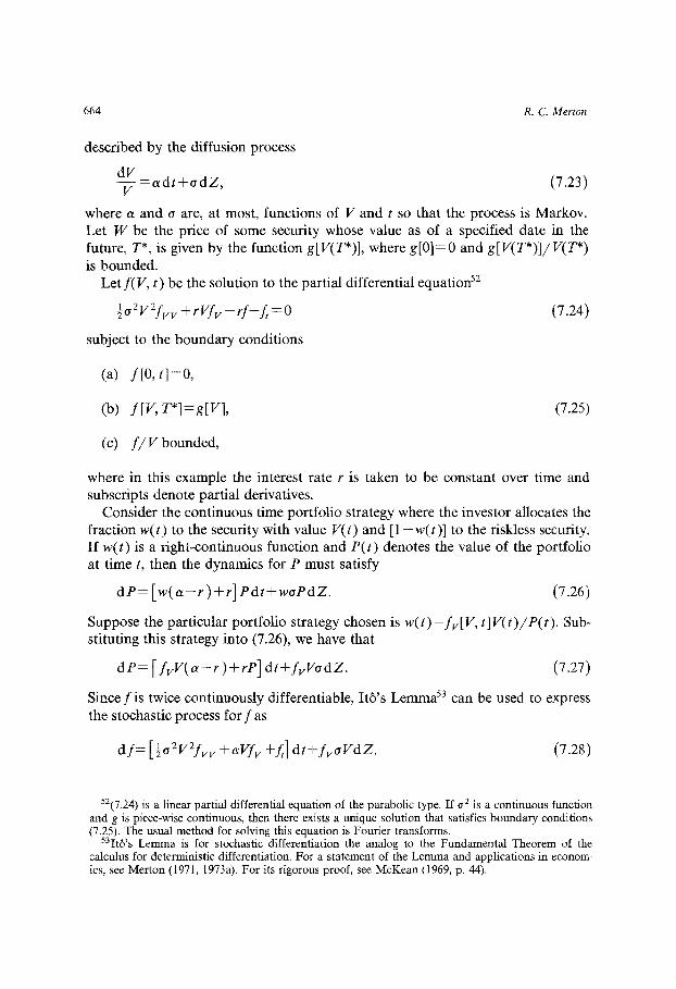
664 R. C. Merton

described by the diffusion process

dV V - a d t + c r d Z , (7.23)

where a and o are, at most, functions of V and t so that the process is Markov. Let W be the price of some security whose value as of a specified date in the future, T*, is given by the function g[V(T*)], where g [0 ]=0 and g[V(T*)]/V(T*) is bounded.

Let f(V, t) be the solution to the partial differential equation 52

l o z V 2 f v V q- rVfv - rf + ft = 0 (7.24)

subject to the boundary conditions

(a) f [O, t ]=O,

(lo) f[V, T*]=g[V], (7.25)

(c) f /Vbounded,

where in this example the interest rate r is taken to be constant over time and subscripts denote partial derivatives.

Consider the continuous time portfolio strategy where the investor allocates the fraction w(t) to the security with value V(t) and [1 - w ( t ) ] to the riskless security. If w(t) is a right-continuous function and P(t) denotes the value of the portfolio at time t, then the dynamics for P must satisfy

d P = [ w ( a - r ) + r ] P d t + w o P d Z . (7.26)

Suppose the particular portfolio strategy chosen is w(t)=fv[V, t]V(t)/P(t). Sub- stituting this strategy into (7.26), we have that

d P = [ f v V ( a - r ) + rP] dt+fvVodZ. (7.27)

Since f is twice continuously differentiable, It6's Lemma 53 can be used to express the stochastic process for f as

d f = [½o2V2fv V +aVfv +ft] dt+fvoVdZ. (7.28)

52(7.24) is a linear partial differential equation of the parabolic type. If o 2 is a continuous function and g is piece-wise continuous, then there exists a unique solution that satisfies boundary conditions (7.25). The usual method for solving this equation is Fourier transforms.

53Itr's Lemma is for stochastic differentiation the analog to the Fundamental Theorem of the calculus for deterministic differentiation. For a statement of the Lemma and applications in economics, see Merton (1971, 1973a). For its rigorous proof, see McKean (1969, p. 44).


But f satisfies (7.24), and therefore (7.28) can be rewritten as

d f = [ fvV(a-r)+rf] dt+fvVodZ. (7.29)

Comparing (7.29) with (7.27), if the initial investment in the portfolio, P(0), is chosen such that P(O)=f[V(O),O], then P(t)=f[V, t] for all V and t<~T *. But P(t) is the value of a feasible portfolio strategy at time t with the properties that P ( t ) = 0 if V( t )=0 and P(T*)=g[V(T*)]. Hence, if the value of the other security, W(t), does not equal P(t) for each t, then there will exist an arbitrage opportunity. Therefore, W( t)----f[V(t), t].

Since g can be a non-linear function, it has been shown that there exists a dynamic portfolio strategy that will exactly replicate the payoff to a non-linear function of the price of the security. The application of this procedure to the debt-equi ty case of (6.13) and (6.14) is immediate. If V denotes the value of the firm, then the debt issue will satisfy (6.24) with g[V]=min[V, B] and the equity will satisfy the same equation but with g[ V] = max[0, V - B ] . In addition, this type of analysis can be used to show that the Modigliani-Miller Theorem (Theorem 6.3) will obtain for non-linear sharing rules) 4 Finally, inspection of (7.24) shows that knowledge of the expected return on V, a, is not required to solve for the values of the various claims, and indeed the only non-observable input required is the variance rate, 0 2 . Moreover, (7.24) often yields closed-form solutions and in those cases where it does not, there exist efficient numerical solution techniques. Hence, this type of analysis has led to a copious theoretical and empirical literature on the pricing of corporate liabilities and contingent claims generally. 55

In summary, the combined assumptions of continuous trading and local state variable changes substantially simplifies the analysis required in the discrete time case. Under these conditions, the crucial non-trivial spanning properties will obtain, and the creation of firm-contingent liabilities will not, in general, affect the equilibrium. An in-depth discussion of the mathematical and economic assumptions required for the valid application of the continuous time analysis is beyond the scope of this paper. However, the required assumptions are rather mild when applied in the context of a securities market. 56 Although continuous trading is only a theoretical proposition, the continuous trading solutions will be an asymptotically valid approximation to the discrete time solution as the trading

54For a proof and extensions to general contingent claim securities, see Merton (1977). 55The literature based on the Black-Scholes type analysis has grown so rapidly that no attempt has

been made here to provide a complete set of references. An excellent survey article is Smith (1976). In addition to the pricing of corporate liabilities, it has been applied to the pricing of loan guarantees, insurance contracts, "dual" funds, term-structure bonds, and even tenure for university professors.

56Merton (forthcoming) discusses in great detail the economic assumptions required for the continuous time methodology. Moreover, all the necessary mathematical tools for manipulation of these models are derived using only elementary probability theory and the calculus.

666 R. C. Merton

interval h becomes small. 57 Indeed, actual securities markets are open virtuaUy every day, and hence the assumption that h is small is not without empirical foundation. In the intertemporal version of the Arrow-Debreu model with complete markets, it is well known that the market need only be open "once" because individuals will have no need for further trade. The continuous trading model is, of course, the opposite extreme. However, the continuous time model appears to have many of the properties of the Arrow-Debreu model without nearly so many securities. Hence, it may be that a good substitute for having so many markets and securities is to have fewer markets and securities but the existing markets open more frequently. The study of this possibility will be left as a topic for future research.

References

Arrow, K. J. (1964), "The role of securities in the optimal allocation of risk bearing", Review of Economic Studies, 31:91-96.

Bawa, V. S. (1975), "Optimal rules for ordering uncertain prospects", Journal of Financial Economics, 2:95-121.

Bertsekas, D. P. (1974), "Necessary and sufficient conditions for existence of an optimal portfolio", Journal of Economic Theory, 8:235-247.

Black, F. (1972), "Capital market equilibrium with restricted borrowing", Journal of Business, 45:444-455. °

Black, F. and M. Scholes (1973), "The pricing of options and corporate liabilities", Journal of Political Economy 81:637-654.

Borch, K. (1969), "A note on uncertainty and indifference curves", Review of Economic Studies, 36:1-4.

Cass, D. and J. E. Stiglitz (1970), "The structure of investor preferences and asset returns, and separability in portfolio allocation: A contribution to the pure theory of mutual funds", Journal of Economic Theory, 2:122-160.

Cox, D. A. and H. D. Miller (1968), The theory of stochastic processes. New York: John Wiley & Sons, Inc.

Debreu, G. (1959), Theory of value. New York: John Wiley & Sons, Inc. Diamond, P. (1967), "The role of a stock market in a general equilibrium model with technological

uncertainty", American Economic Review, 57:759-776. Dreyfus, S. E. (1965), Dynamic programming and the calculus of variations. New York: Academic

Press. Eckeru, S. and R. Wilson (1974), "On the theory of the firm in an economy with incomplete markets",

Bell Journal of Economics and Management Science, 5:171-180. Fama, E. (1965), "The behavior of stock market prices", Journal of Business 38:34-105. Fama, E. (1970a), "Efficient capital markets: A review of theory and empirical work", Journal of

Finance, 25:383-417. Fama, E. (1970b), "Multiperiod consumption-investment decisions", American Economic Review,

60:163-174.

57See Samuelson (1970) and Merton and Samuelson (1974). In Merton (1975a, p. 663) there is a brief discussion of the special cases in which the limiting discrete time solutions do not approach the continuous time solutions.


Fama, E. (1972), "Perfect competition and optimal production decisions under uncertainty", Bell Journal of Economics and Management Science, 3:509-530.

Fama, E. (1978), "The effects of a firm's investment and financing decisions on the welfare of its securityholders', American Economic Review, 68.

Fama, E. and A. B. Laffer (1972), "The number of firms and competition", American Economic Review, 62:670-674.

Farrar, D. E. (1962), The investment decision under uncertainty. Englewood Cliffs, New Jersey: Prentice Hall,

Farrell, J. L. (1974), "Analyzing covariation of returns to determine homogeneous stock groupings", Journal of Business, 47:186-207.

Feeney, G. J., and D. Hester (1967), "Stock market indices: A principal components analysis", in: D. Hester and J. Tobin, eds., Risk aversion and portfolio choice. New York: John Wiley & Sons, Inc.

Feldstein, M. S. (1969), "Mean-variance analysis in the theory of liquidity preference and portfolio selection", Review of Economic Studies, 36:5- l 2.

Feller, W. (1966), An introduction to probability theory and its applications, Vol. 2. New York: John Wiley & Sons, Inc.

Fischer, S. (1972), "Assets, contingent commodities, and the Slutsky equations", Econometrica, 40:371-385.

Friend, I. and J. Bicksler (eds.) (1975), Studies in risk and return, Vols. I & II. Cambridge, Mass: Ballinger.

Goldman, M. B. (1974), "A negative report on the 'near-optimality' of the max-expected-log policy as applied to bounded utilities for long-lived programs", Journal of Financial Economics, 1:97-103.

Grossman, S. (1976), "On the efficiency of competitive stock markets where traders have diverse information", Journal of Finance, 31:573-585.

Grossman, S. and J. E. Stiglitz (1976), "Information and competitive price systems", American Economic Review, 66:246-253.

Hadar, J. and W. R. Russell (1969), "Rules for ordering uncertain prospects", American Economic Review, 59:25-34.

Hadar, J. a~d W. R. Russell (1971), "Stochastic dominance and diversification", Journal of Economic Theory, 3:288-305.

Hakansson, N. (1970), "Optimal investment and consumption strategies under risk for a class of utility functions", Econometrica, 38:587-607.

Hanoch, G, and H. Levy (1969), "The efficiency analysis of choices involving risk", Review of Economic Studies, 36:335-346.

Hardy, G. H., J. E. Littlewood, and G. P~51ya. (1959), Inequalities. Cambridge: Cambridge University Press.

Hart, O. (1975), "On the optimality of equilibrium when the market structure is incomplete", Journal of Economic Theory, 11:418-443.

Hcrstein, I. and J. Milnor. (1953), "An axiomatic approach to measurable utility", Econometrica, 21:291-297.

Hirshleifer, J. (1965), "Investment decision under uncertainty: Choice-theoretic approaches", Quarterly Journal of Economics 79:509-536.

Hirshleifer, J. (1966), "Investment decisions under uncertainty: Applications of the state-preference approach", Quarterly Journal of Economics, 80:252-277.

Hirshleifer, J. (1970), Investment, interest and capital. Englewood Cliffs, New Jersey: Prentice-Hall. Hirschleifer, J. (1973), "Where are we in the theory of information", American Economic Review,

63:31-39. It6, K. and H. P. McKean, Jr. (1964), Diffusion processes and their sample paths. New York:

Academic Press. Jensen, M. C. (ed.). (1972), Studies in the theory of capital markets. New York: Praeger Publishers. Jensen, M. C. (ed.). (1972), "Capital markets: Theory and evidence", Bell Journal of Economics and

Management Science, 3:357-398. Jensen, M. C. (ed.) and J. B. Long, Jr. (1972), "Corporate investment under uncertainty and Pareto

optimality in the capital markets", Bell Journal of Economics and Management Science, 3:15 I - 174. King, B. R. (1966), "Market and industry factors in stock price behavior", Journal of Business, 39

Supplement: 139-190.

668 R. C. Merton

Ktthn, H. W. and A. W. Tucker. (1951), "Nonlinear programming", in: J. Neyman, ed., Proceedings of the Second Berkeley Symposium of mathematical statistics and probability. Berkeley: University of California Press.

Kushner, H. J. (1967), Stochastic stability and control. New York: Academic Press. Latane, H. (1959), "Criteria for choice among risky ventures", Journal of Political Economy,

67:144-155. Leland, H. (1972), "On the existence of optimal policies under uncertainty", Journal of Economic

Theory, 4:35-44. Leland, H. (1974), "Production theory and the stock market", Bell Journal of Economics and

Management Science, 5:125-144. Lintner, J. (1965), "The valuation of risk assets and the selection of risky investments in stock

portfolios and capital budgets", Review of Economics and Statistics, 47:13-37. Livingston, M. (1977), "Industry movements of common stocks", Journal of Finance, 32:861-874. Markowitz, H. (1959), Portfolio selection: Efficient diversification of investment. New York: John

Wiley & Sons, Inc. Markowitz, H. (1976), "Investment for the long run: New evidence for an old rule", Journal of

Finance, 31 : 1273-1286. McKean, Jr., H. P. (1969), Stochastic integrals. New York: Academic Press. McShane, E. J. (1974), Stochastic calculus and stochastic models. New York: Academic Press. Merton, R. C. (1969), "Lifetime portfolio selection under uncertainty: The continuous-time case",

Review of Economics and Statistics, 51:247-257. Merton, R. C. (1971), "Optimum consumption and portfolio rules in a continuous time model",

Journal of Economic Theory, 3:373-413. Merton, R. C. (1972), "An analytic derivation of the efficient portfolio frontier", Journal of Financial

and Quantitative Analysis, 7:185 l - 1872. Merton, R. C. (1973a) "Theory of rational option pricing", Bell Journal of Economics and Manage-

ment Science, 4:141-183. Merton, R. C. (1973b), "An intertemporal capital asset pricing model", Econometrica, 41:867-887. Merton, R. C. (L975a), "Theory of finance from the perspective of continuous time", Journal of

Financial and Quantitative Analysis, 10:659-674. Merton, R. C. (1975b), "A reexamination of the capital asset pricing model", in: Friend and Bicksler,

eds. (1975). Merton, R. C. (1977), "On the pricing of contingent claims and the Modigliani-Miller theorem",

Journal of Financial Economics, 5:241-249. Merton, R. C. (forthcoming), "On the mathematics and economic assumptions of continuous-time

financial models", in: W. F. Sharpe, ed., Financial Economics: Essays in Honor of Paul Cootner. Englewood Cliffs: Prentice Hall Inc.

Merton, R. C. and P. A. Samuelson (1974), "Fallacy of the log-normal approximation to optimal portfolio decision making over many periods", Journal of Financial Economics, 1:67-94.

Merton, R. C. and M. G. Subrahmanyam (1974), "The optimality of a competitive stock market", Bell Journal of Economics and Management Science, 5:145-170.

Miller, M. H. (1977), "Debt and taxes", Journal of Finance, 32:261-276. Miller, M. H. and F. Modigliani (1958), "The cost of capital, corporation finance, and the theory of

investment", American Economic Review, 48:261-297. Mossin, J. (1966), "Equilibrium in a capital asset market", Econometrica, 35:768-783. Myers, S. C. (1968), "A lime-state-preference model of security valuation", Journal of Financial and

Quantitative Analysis, 3: l - 33. Pratt, J. W. (1964), "Risk aversion in the small and in the large", Econometrica, 32:122-136. Radner, R. (1970), "Problems in the theory of markets under uncertainty", American Economic

Review, 60:454-460. Radner, R. (1974), "A note on the unanimity of stockholders' preferences among alternative

production plans: A reformulation of the Eckern-Wilson model", Bell Journal of Economics and Management Science, 5:181 - 186.

Richard, S. (1975), "Optimal consumption, portfolio, and life insurance rules for an uncertain lived individual in a continuous-time model", Journal of Financial Economics. 2:187-204.


Ross, S. (1976), "Arbitrage theory of capital asset pricing", Journal of Economic Theory 13: 341 - 360. Ross, S. (1978), "Mutual fund separation in financial theory: The separating distributions", Journal of

Economic Theory. 17:254- 286. Rothschild, M. and J. E. Stiglitz (1970), "Increasing risk I: A definition", Journal of Economic

Theory, 2:225-243. Rothschild, M. and J. E. Stiglitz (1971), "Increasing risk II: Its economic consequences", Journal of

Economic Theory, 3:66- 84. Rubinstein, M. (1976), "The strong case for the generalized logarithmic utility model as the premier

model of financial markets", Journal of Finance, 31:551-572. Samuelson, P. A. (1965), "Proof that properly anticipated prices fluctuate randomly", Industrial

Management Review, 6:41-49. Reprinted in Samuelson (1972). Samuelson, P. A. (1967), "General proof that diversification pays", Journal of Financial and

Quantitative Analysis, 2:1-13. Reprinted in Samuelson (1972). Samuelson, P. A. (1969), "Lifetime portfolio selection by dynamic stochastic programming", Review

of Economics and Statistics, 51:239-246. Reprinted in Samuelson (1972). Samuelson, P. A. (1970), "The fundamental approximation theory of portfolio analysis in terms of

means, variances, and higher moments", Review of Economic Studies, 37:537-542. Reprinted in Samuelson (1972).

Samuelson, P. A. (1971), "The 'fallacy' of maximizing the geometric mean in long sequences of investing or gambling", Proceedings of the National Academy of Sciences, 68:2493-2496. Re- printed in Samuelson (1972).

Samuelson, P. A. (1972), in: R. C. Merton, ed., The collected scientific papers of Paul A. Sameulson, Vol III. Cambridge: M.I.T. Press.

Samuelson, P. A. (1973), "Proof that properly discounted present values of assets vibrate randomly", Bell Journal of Economics and Management Science, 4:369-374.

Samuelson, P. A. (1977), "St. Petersburg paradoxes: Deranged, dissected, and historically described", Journal of Economic Literature, 15:24- 55.

Sharpe, W. (1964), "Capital asset prices: A theory of market equilibrium under conditions of risk", Journal of Finance, 19:425 - 442.

Sharpe, W. (1970), Portfolio theory and capital markets. New York: McGraw-Hill. Smith, Jr., C. W. (1976), "Option pricing: A review", Journal of Financial Economics, 3:3-52. Stiglitz, J. E. (1969), "A re-examination of the Modigliani-Miller theorem", American Economic

Review, 59:78-93. Stiglitz, J. E. (1972), "On the optimality of the stock market allocation of investment", Quarterly

Journal of Economics, 86:25-60. Stiglitz, J. E. (1974), "On the irrelevance of corporate financial policy", American Economic Review,

64:851-866. Tobin, J. (1958), "Liquidity preference as behavior towards risk", Review of Economic Studies,

25:68-85. Tobin, J. (1969), "'Comment on Borch and Feldstein", Review of Economic Studies, 36:13-14. Von Neumann, J. and O. Morgenstern (1947), Theory of games and economic behavior, 2nd edn.

Princeton: Princeton University Press.

on the microeconomic theory of investment … theory of investment und… · *this paper is not a...

Documents