on the maxima of heterogeneous gamma variables with different shape and scale parameters

MetrikaDOI 10.1007/s00184-013-0466-4

On the maxima of heterogeneous gamma variableswith different shape and scale parameters

Peng Zhao · Yiying Zhang

Received: 1 December 2012© Springer-Verlag Berlin Heidelberg 2013

Abstract In this article, we study the stochastic properties of the maxima from twoindependent heterogeneous gamma random variables with different both shape para-meters and scale parameters. Our main purpose is to address how the heterogeneity ofa random sample of size 2 affects the magnitude, skewness and dispersion of the max-ima in the sense of various stochastic orderings. Let X1 and X2 be two independentgamma random variables with Xi having shape parameter ri > 0 and scale parameterλi , i = 1, 2, and let X∗

1 and X∗2 be another set of independent gamma random variables

with X∗i having shape parameter r∗

i > 0 and scale parameter λ∗i , i = 1, 2. Denote

by X2:2 and X∗2:2 the corresponding maxima, respectively. It is proved that, among

others, if (r1, r2)majorize (r∗1 , r

∗2 ) and (λ1, λ2)weakly majorize (λ∗

1, λ∗2), then X2:2 is

stochastically larger that X∗2:2 in the sense of the likelihood ratio order. We also study

the skewness according to the star order for which a very general sufficient conditionis provided, using which some useful consequences can be obtained. The new resultsestablished here strengthen and generalize some of the results known in the literature.

Keywords Gamma distribution · Likelihood ratio order · Hazard rate order ·Dispersive order · Star order · Majorization · p-Larger order · Parallel system

This work was supported by National Natural Science Foundation of China (11001112), the FundamentalResearch Funds for the Central Universities (lzujbky-2011-122), and A Project Funded by the PriorityAcademic Program Development of Jiangsu Higher Education Institutions.

P. Zhao (B)School of Mathematics and Statistics, Jiangsu Normal University,Xuzhou 221116, Chinae-mail: [email protected]

Y. ZhangSchool of Mathematics and Statistics, Lanzhou University,Lanzhou 730000, China

123

P. Zhao, Y. Zhang

1 Introduction

In the literature, order statistics play a prominent role in statistical inference, reliabilitytheory, life testing, operations research, and many other areas. It is well known thatthe k-th order statistic Xk:n from sample X1, . . . , Xn corresponds to the lifetime of a(n − k + 1)-out-of-n system, which is a very popular structure of redundancy in fault-tolerant systems that have been studied extensively. In particular, Xn:n and X1:n denotethe lifetimes of parallel and series systems, respectively. There are large amountsof papers appeared on various aspects of order statistics when the observations areindependent and identically distributed (i.i.d.), but for the case when observations arenon-i.i.d., not too much work is available in the literature due to the complexity of thedistribution theory; see, for example, David and Nagaraja (2003), Balakrishnan andRao (1998a,b) and Balakrishnan (2007) for comprehensive discussions on this topic.

Pledger and Proschan (1971) may be the first to stochastically compare the order sta-tistics arising from heterogeneous exponential variables. After that, many researchershave paid their attentions to this topic, including Proschan and Sethuraman (1976),Kochar and Rojo (1996), Dykstra et al. (1997), Khaledi and Kochar (2000), Bon andPaltanea (2006), Kochar and Xu (2007), Kochar and Xu (2011), Paltanea (2008), Zhaoand Balakrishnan (2009a), Zhao and Balakrishnan (2011a,b), Zhao et al. (2009), Jooand Mi (2010), Mao and Hu (2010), Khaledi et al. (2011), and references therein. LetX1, . . . , Xn be independent exponential random variables with Xi having hazard rateλi , i = 1, . . . , n. Let X∗

1, . . . , X∗n be another set of independent exponential random

variables with X∗i having hazard rate λ∗

i . Then, Pledger and Proschan (1971) showed,for 1 ≤ k ≤ n, that

(λ1, . . . , λn)m� (λ∗

1, . . . , λ∗n) �⇒ Xk:n ≥st X∗

k:n . (1)

Formal definitions of stochastic orderings will be given in the next section. Proschanand Sethuraman (1976) strengthened this result from componentwise stochastic order-ing to multivariate stochastic ordering, and Khaledi and Kochar (2000) partiallyimproved (1) under a weaker condition as

(λ1, . . . , λn)p� (λ∗

1, . . . , λ∗n) �⇒ Xn:n ≥st X∗

n:n . (2)

Moreover, Khaledi et al. (2011) extended the result in (2) to the scale model whichincludes gamma as its special case.

With the help of a counterexample, Boland et al. (1994) showed that (1) can not bestrengthened from the usual stochastic order to the hazard rate order when n > 2; butfor the case when n = 2, they proved that

(λ1, λ2)m� (λ∗

1, λ∗2) �⇒ X2:2 ≥hr X∗

2:2. (3)

Dykstra et al. (1997) further improved (3) from the hazard rate order to the likelihoodratio order as

123

On the maxima of heterogeneous gamma variables

(λ1, λ2)m� (λ∗

1, λ∗2) �⇒ X2:2 ≥lr X∗

2:2. (4)

Under the condition λ1 ≤ λ∗1 ≤ λ∗

2 ≤ λ2, Joo and Mi (2010) proved that

(λ1, λ2)w� (λ∗

1, λ∗2) �⇒ X2:2 ≥hr X∗

2:2. (5)

Zhao and Balakrishnan (2011a,b) further strengthened all the results above in (3)–(5)and obtained two characterization results, i.e., under the conditionλ1 ≤ λ∗

1 ≤ λ∗2 ≤ λ2,

that

(λ1, λ2)w� (λ∗

1, λ∗2) ⇐⇒ X2:2 ≥lr X∗

2:2 (6)

and

(λ1, λ2)p� (λ∗

1, λ∗2) ⇐⇒ X2:2 ≥hr X∗

2:2. (7)

Gamma distribution is one of the most commonly used distributions in reliabilityand life testing. If X is a gamma random variable with shape parameter r and scaleparameter λ, in its standard form X has the probability density function

f (x; r, λ) = λr

�(r)xr−1e−λx , x > 0.

It is an extremely flexible family of distributions with decreasing, constant, and increas-ing failure rates when 0 < r < 1, r = 1 and r > 1, respectively. In this paper, we willfocus our attentions on the maximum order statistic from two gamma observations,i.e., the lifetime of a parallel system consisting of two independent heterogeneousgamma components with different both shape and scale parameters. First, we providean example to illustrate potential application of this research.

Consider a typical scenario in the context of reliability theory. Now we havea parallel system with two components wherein each component is subject toshocks occurred at times in accordance with a Poisson process with rate 1. Everyshock affects only one of the components and it affects components i with proba-bility pi (p1 + p2 = 1). For any component i , it can endure at most ri −1 shocksbefore failing (one possibility being that with probability pi a shock knocks outthe component for position i in which there are ri − 1 standby redundancies).Let Ti (i = 1, 2) denote the failure time of component i , and then the Ti ’s areindependent gamma random variables with Ti having its shape parameter ri andscale parameter pi . As a result, T = max{T1, T2}, the maximum from inde-pendent gamma random variables T1 and T2, is the lifetime of such a parallelsystem. It would be of great interest for a reliability engineer to investigate thestochastic properties of T .

Let X1, X2 be independent gamma random variables with Xi having shape para-meter ri and scale parameter λi , i = 1, 2, and X∗

1, X∗2 be another set of independent

123

P. Zhao, Y. Zhang

gamma random variables with X∗i having shape parameter r∗

i and scale parameter λ∗i ,

i = 1, 2. Suppose r1 ≥ r2, r∗1 ≥ r∗

2 and λ1 ≤ λ∗1 ≤ λ∗

2 ≤ λ2. It is showed that

(r1, r2)m� (r∗

1 , r∗2 ), (λ1, λ2)

w� (λ∗1, λ

∗2) �⇒ X2:2 ≥lr X∗

2:2. (8)

We also study the skewness according to the star order (see Definition 2.3 in Sect. 2)which reveals the departure of a distribution from symmetry wherein one tail of thedensity is more stretched out than the other. It is proved that, if r1 ≥ r2, λ1 ≤ λ2 andλ∗

1 ≤ λ∗2, then

λ2

λ1≥ λ∗

2

λ∗1

�⇒ X2:2 ≥� X∗2:2. (9)

With the help of (9), it is proved, if r2 ≤ r1 and λ1 ≤ λ∗1 ≤ λ∗

2 ≤ λ2, then,

(λ1, λ2)w� (λ∗

1, λ∗2) �⇒ X2:2 ≥disp X∗

2:2. (10)

These new results in (8)–(10) generalize and strengthen all the results in (3)–(6)established earlier in the literature for the exponential case. It should be also metionedthat Zhao (2011) and Zhao and Balakrishnan (2012b) established some results similarto those in (8) and (10) for the special case when having same shape parameters.

2 Definitions

In this section, we recall some notions of stochastic orders, and majorization andrelated orders. Throughout this paper, the term increasing is used for monotone non-decreasing and decreasing is used for monotone non-increasing.

2.1 Stochastic orders

Definition 2.1 For two random variables X and Y with densities fX and fY , anddistribution functions FX and FY , respectively, let F X = 1 − FX and FY = 1 − FY

be the corresponding survival functions. Then, X is said to be smaller than Y in

(i) the likelihood ratio order (denoted by X ≤lr Y ) if fY (x)/ fX (x) is increasing inx ;

(ii) the hazard rate order (denoted by X ≤hr Y ) if FY (x)/F X (x) is increasing in x ;(iii) the reversed hazard rate order (denoted by X ≤rh Y ) if FY (x)/FX (x) is increasing

in x ;(iv) the stochastic order (denoted by X ≤st Y ) if FY (x) ≥ F X (x).

For comprehensive discussions and applications on various stochastic orders above,one may refer to Shaked and Shanthikumar (2007) and Müller and Stoyan (2002). Oneof the basic criteria for comparing variability in probability distributions is dispersiveorder.

123


Definition 2.2 A random variable X is said to be less dispersed than another randomvariable Y (denoted by X ≤disp Y ) if

F−1(v)− F−1(u) ≤ G−1(v)− G−1(u)

for 0 ≤ u ≤ v ≤ 1, where F−1 and G−1 are the right continuous inverses of thedistribution functions F and G of X and Y , respectively.

Definition 2.3 X is said to be smaller than Y in the star order (denoted by X ≤� Y )if G−1 F(x)/x is increasing in x on the support of X .

The star order is also called the more IFRA (increasing failure rate in average) orderin reliability theory and is one of the partial orders which are scale invariant.

The function

L X (u) = 1

EX

F−1(u)∫

−∞xdF(x)

is called Lorenz curve in the economic literature, which is often used to describe theinequality in incomes. Based on Lorenz curve, the Lorenz order has been proposed ineconomics to compare income inequalities.

Definition 2.4 X is said to smaller than Y in the Lorenz order (denoted byX ≤Lorenz Y ) if

1

EX

F−1(u)∫

−∞xdF(x) ≤ 1

EY

G−1(u)∫

−∞xdG(x), u ∈ (0, 1].

It is known from Marshall and Olkin (2007) that

X ≤� Y �⇒ X ≤Lorenz Y.

Detailed discussions of the star order and the Lorenz order can be found in Barlowand Proschan (1975) and Marshall and Olkin (2007).

2.2 Majorization and related orders

The notion of majorization is quite useful in establishing various inequalities. Letx(1) ≤ · · · ≤ x(n) be the increasing arrangement of the components of the vectorx = (x1, . . . , xn).

123

P. Zhao, Y. Zhang

Definition 2.5 (i) A vector x = (x1, . . . , xn) ∈ �n is said to majorize another vector

y = (y1, . . . , yn) ∈ �n (written as xm� y) if

j∑i=1

x(i) ≤j∑

i=1

y(i) for j = 1, . . . , n − 1,

and∑n

i=1 x(i) = ∑ni=1 y(i);

(ii) A vector x ∈ �n is said to weakly supermajorize another vector y ∈ �n (written

as xw� y) if

j∑i=1

x(i) ≤j∑

i=1

y(i) for j = 1, . . . , n;

(iii) A vector x ∈ �n+ is said to be p-larger than another vector y ∈ �n+ (written as

xp� y) if

j∏i=1

x(i) ≤j∏

i=1

y(i) for j = 1, . . . , n;

(iv) A vector x ∈ �n+ is said to reciprocal majorize another vector y ∈ �n+ (written

as xrm� y) if

j∑i=1

1

x(i)≥

j∑i=1

1

y(i)for j = 1, . . . , n.

It is evident that xm� y implies x

w� y, and xp� y is equivalent to log(x)

w� log(y),where log(x) is the vector of logarithms of the coordinates of x. It is well known that

xw� y �⇒ x

p� y �⇒ xrm� y

for any two non-negative vectors x and y. For more details on majorization, p-largerand reciprocal majorization orders and their applications, one may refer to Marshallet al. (2011), Bon and Paltanea (1999), and Zhao and Balakrishnan (2009b).

3 Likelihood ratio ordering

We first present several lemmas that will be used to establish the principal results inthis section. The first one turns out to be a useful tool for showing the monotonicityof a fraction whose numerator and denominator are integrals or summations.

123


Lemma 3.1 (Misra and Meulen 2003) Let � be a subset of a real line and U be anonnegative random variable having a cumulative distribution function (c.d.f) belong-ing to a stochastically ordered family P = {H(·|θ), θ ∈ �}; that is, for θ1, θ2 ∈ �,H(·|θ1) ≤st [≥st]H(·|θ2)whenever θ1 < θ2. Suppose a real functionψ(u, θ) on �·�is measurable in u for each θ such that Eθ [ψ(U, θ)] exists. Then the following hold:

(i) Eθ [ψ(U, θ)] is increasing in θ if ψ(u, θ) is increasing in θ and increasing[decreasing] in u;

(ii) Eθ [ψ(U, θ)] is decreasing in θ if ψ(u, θ) is decreasing in θ and decreasing[increasing] in u.

Lemma 3.2 (Zhao 2011) For r > 0 and y ∈ �+, the function

f (x) = x + yr−1e−xy∫ y

0ur−1e−xudu

is increasing in x ∈ �+.

The technical details of the proofs of following Lemmas 3.3–3.5 are deferred toAppendix.

Lemma 3.3 For λ > 0 and t ∈ �+, the function

g(r) = r − tr e−λt

∫ t

0ur−1e−λudu

is increasing in r ∈ �+.

Lemma 3.4 Suppose 0 < λ1 ≤ λ2, 0 < λ∗1 ≤ λ∗

2 and a ≥ 0. If (λ1, λ2)m� (λ∗

1, λ∗2),

then the function

ϕ(y, t) = e−λ1 yt + (1 − y)ae−λ2 yt

e−λ∗1 yt + (1 − y)ae−λ∗

2 yt

is increasing in both t ∈ �+ and y ∈ (0, 1).

Lemma 3.5 Suppose 0 < r2 ≤ r1, 0 < r∗2 ≤ r∗

1 and b ≥ 0. If (r1, r2)m� (r∗

1 , r∗2 ),

then the function

ζ(y, t) = yr2 eb(1−y)t + yr1

yr∗2 eb(1−y)t + yr∗

1

is increasing in t ∈ �+ while is decreasing in y ∈ (0, 1).

We are now ready to present the main results of this section.

123

P. Zhao, Y. Zhang

Theorem 3.6 Let (X1, X2) be a vector of independent gamma random variables withrespective shape parameters r1 and r2 and respective scale parameters λ1 and λ, andlet (Y1,Y2) be another vector of independent gamma random variables with respectiveshape parameters r1 and r2 and respective scale parameters λ2 and λ. Suppose r1 ≥ r2and λ ≥ λ2 ≥ λ1. Then, it holds that X2:2 ≥lr Y2:2.

Proof Denote by fi [gi ] and Fi [Gi ] the density and distribution functions of Xi [Yi ],respectively, and denote by rX2:2 and rY2:2 the reversed hazard rate functions of X2:2 andY2:2, respectively. To reach the desired result, we will show that X2:2 ≥rh Y2:2 and theratio of their reversed hazard rate function (i.e., φ(t) = rX2:2(t)/rY2:2(t)) is increasingin t ∈ �+ in accordance with Theorem 1.C.4(b) of Shaked and Shanthikumar (2007).We first notice that

rX2:2(t) = rX1(t)+ rX2(t) and rY2:2(t) = rY1(t)+ rY2(t).

Since rX2(t) = rY2(t) and λ2 ≥ λ1 implies that X1 ≥rh Y1 (i.e., rX1(t) ≥ rY1(t)), wehave rX2:2(t) ≥ rY2:2(t). In what follows we need to show that the function

φ(t) =

⎛⎜⎜⎝ tr1−r2 e−λ1t

∫ t

0ur1−1e−λ1udu

+ e−λt

∫ t

0ur2−1e−λudu

⎞⎟⎟⎠

×

⎛⎜⎜⎝ tr1−r2 e−λ2t

∫ t

0ur1−1e−λ2udu

+ e−λt

∫ t

0ur2−1e−λudu

⎞⎟⎟⎠

−1

is increasing in t ∈ �+. Taking the the derivative of φ(t) with respect to t gives riseto

φ′(t)

⎛⎜⎜⎝ tr1−r2 e−λ2t

∫ t

0ur1−1e−λ2udu

+ e−λt

∫ t

0ur2−1e−λudu

⎞⎟⎟⎠

2

=

⎡⎢⎢⎣−

⎛⎜⎜⎝λ1 − r1 − r2

t+ tr1−1e−λ1t

∫ t

0ur1−1e−λ1udu

⎞⎟⎟⎠ tr1−r2 e−λ1t

∫ t

0ur1−1e−λ1udu

−

⎛⎜⎜⎝λ+ tr2−1e−λt

∫ t

0ur2−1e−λudu

⎞⎟⎟⎠ e−λt

∫ t

0ur2−1e−λudu

⎤⎥⎥⎦

×

⎛⎜⎜⎝ tr1−r2 e−λ2t

∫ t

0ur1−1e−λ2udu

+ e−λt

∫ t

0ur2−1e−λudu

⎞⎟⎟⎠

123


−

⎡⎢⎢⎣−

⎛⎜⎜⎝λ2 − r1 − r2

t+ tr1−1e−λ2t

∫ t

0ur1−1e−λ2udu

⎞⎟⎟⎠ tr1−r2 e−λ2t

∫ t

0ur1−1e−λ2udu

−

⎛⎜⎜⎝λ+ tr2−1e−λt

∫ t

0ur2−1e−λudu

⎞⎟⎟⎠ e−λt

∫ t

0ur2−1e−λudu

⎤⎥⎥⎦

×

⎛⎜⎜⎝ tr1−r2 e−λ1t

∫ t

0ur1−1e−λ1udu

+ e−λt

∫ t

0ur2−1e−λudu

⎞⎟⎟⎠ = A + B, say,

where

A =

⎛⎜⎜⎝λ2 + tr1−1e−λ2t

∫ t

0ur1−1e−λ2udu

− λ1 − tr1−1e−λ1t

∫ t

0ur1−1e−λ1udu

⎞⎟⎟⎠

× t2(r1−r2)e−(λ1+λ2)t∫ t

0ur1−1e−λ1udu

∫ t

0ur1−1e−λ2udu

and

B =

⎡⎢⎢⎣

⎛⎜⎜⎝λ+ tr2−1e−λt

∫ t

0ur2−1e−λudu

+ r1 − r2

t− λ1 − tr1−1e−λ1t

∫ t

0ur1−1e−λ1udu

⎞⎟⎟⎠

× tr1−r2 e−(λ1+λ)t∫ t

0ur1−1e−λ1udu

∫ t

0ur2−1e−λudu

⎤⎥⎥⎦

+

⎡⎢⎢⎣

⎛⎜⎜⎝λ2 + tr1−1e−λ2t

∫ t

0ur1−1e−λ2udu

− r1 − r2

t− λ− tr2−1e−λt

∫ t

0ur2−1e−λudu

⎞⎟⎟⎠

× tr1−r2 e−(λ2+λ)t∫ t

0ur1−1e−λ2udu

∫ t

0ur2−1e−λudu

⎤⎥⎥⎦ .

From Lemma 3.2, we have A ≥ 0. We next show that B ≥ 0. Since

123

P. Zhao, Y. Zhang

e−λt

∫ t

0ur−1e−λudu

is decreasing in λ, it follows that

e−(λ1+λ)t∫ t

0ur1−1e−λ1udu

∫ t

0ur2−1e−λudu

≥ e−(λ2+λ)t∫ t

0ur1−1e−λ2udu

∫ t

0ur2−1e−λudu

. (11)

On the other hand, upon applying Lemmas 3.2 and 3.3, respectively, we have thefollowing two inequalities:

λ+ tr1−1e−λt

∫ t

0ur1−1e−λudu

≥ λ1 + tr1−1e−λ1t

∫ t

0ur1−1e−λ1udu

(12)

and

r1 − tr1 e−λt

∫ t

0ur1−1e−λudu

≥ r2 − tr2 e−λt

∫ t

0ur2−1e−λudu

. (13)

Combining inequalities (12) and (13), we now have

λ+ tr2−1e−λt

∫ t

0ur2−1e−λudu

+ r1 − r2

t− λ1 − tr1−1e−λ1t

∫ t

0ur1−1e−λ1udu

=

⎡⎢⎢⎣λ+ tr1−1e−λt

∫ t

0ur1−1e−λudu

−

⎛⎜⎜⎝λ1 + tr1−1e−λ1t

∫ t

0ur1−1e−λ1udu

⎞⎟⎟⎠

⎤⎥⎥⎦

+1

t

⎡⎢⎢⎣r1 − tr1e−λt

∫ t

0ur1−1e−λudu

−

⎛⎜⎜⎝r2 − tr2 e−λt

∫ t

0ur2−1e−λudu

⎞⎟⎟⎠

⎤⎥⎥⎦ ≥ 0.

123


Then, it holds from (11) and (12) that

B ≥

⎡⎢⎢⎣

⎛⎜⎜⎝λ+ tr2−1e−λt

∫ t

0ur2−1e−λudu

+ r1 − r2

t− λ1 − tr1−1e−λ1t

∫ t

0ur1−1e−λ1udu

⎞⎟⎟⎠

× tr1−r2 e−(λ2+λ)t∫ t

0ur1−1e−λ2udu

∫ t

0ur2−1e−λudu

⎤⎥⎥⎦

+

⎡⎢⎢⎣

⎛⎜⎜⎝λ2 + tr1−1e−λ2t

∫ t

0ur1−1e−λ2udu

− r1 − r2

t− λ− tr2−1e−λt

∫ t

0ur2−1e−λudu

⎞⎟⎟⎠

× tr1−r2 e−(λ2+λ)t∫ t

0ur1−1e−λ2udu

∫ t

0ur2−1e−λudu

⎤⎥⎥⎦

sgn=λ2 + tr1−1e−λ2t

∫ t

0ur1−1e−λ2udu

− λ1 − tr1−1e−λ1t

∫ t

0ur1−1e−λ1udu

≥ 0,

which means that φ′(t) ≥ 0, i.e., φ(t) is increasing in t ∈ �+. Hence, the proof iscompleted. �Theorem 3.7 Let (X1, X2) be a vector of independent gamma random variables withrespective shape parameters r1 and r2 and respective scale parameters λ1 and λ2,and let (X∗

1, X∗2) be another vector of independent gamma random variables with

respective shape parameters r1 and r2 and respective scale parameters λ∗1 and λ∗

2.Suppose r1 ≥ r2, λ2 ≥ λ1 and λ∗

2 ≥ λ∗1. Then,

(λ1, λ2)m� (λ∗

1, λ∗2) �⇒ X2:2 ≥lr X∗

2:2.

Proof Denote by fX2:2(t) [ fX∗2:2(t)] the density function of X2:2 [X∗

2:2]. It suffices toprove that �(t) = fX2:2(t)/ fX∗

2:2(t) is increasing in t ∈ �+. Note that

�(t)=λ

r11

�(r1)tr1−1e−λ1t

∫ t

0

λr22

�(r2)ur2−1e−λ2udu+ λ

r22

�(r2)tr2−1e−λ2t

∫ t

0

λr11

�(r1)ur1−1e−λ1udu

(λ∗1)

r1

�(r1)tr1−1e−λ∗

1 t∫ t

0

(λ∗2)

r2

�(r2)ur2−1e−λ∗

2udu+ (λ∗2)

r2

�(r2)tr2−1e−λ∗

2 t∫ t

0

(λ∗1)

r1

�(r1)ur1−1e−λ∗

1udu

∝

∫ 1

0

[yr2−1e−(λ1+λ2 y)t + yr1−1e−(λ2+λ1 y)t

]dy

∫ 1

0

[yr2−1e−(λ∗

1+λ∗2 y)t + yr1−1e−(λ∗

2+λ∗1 y)t

]dy

123

P. Zhao, Y. Zhang

=1∫

0

yr2−1e−(λ1+λ2 y)t + yr1−1e−(λ2+λ1 y)t

∫ 1

0

[yr2−1e−(λ∗

1+λ∗2 y)t + yr1−1e−(λ∗

2+λ∗1 y)t

]dy

dy

=1∫

0

c(t)[

yr2−1e−(λ∗1+λ∗

2 y)t + yr1−1e−(λ∗2+λ∗

1 y)t]

× yr2−1e−(λ1+λ2 y)t + yr1−1e−(λ2+λ1 y)t

yr2−1e−(λ∗1+λ∗

2 y)t + yr1−1e−(λ∗2+λ∗

1 y)tdy

=1∫

0

h(y|t)ψ(y, t)dy

= Etψ(Y, t),

where

c(t) = 1∫ 1

0

[yr2−1e−(λ∗

1+λ∗2 y)t + yr1−1e−(λ∗

2+λ∗1 y)t

]dy

and

ψ(y, t) = yr2−1e−(λ1+λ2 y)t + yr1−1e−(λ2+λ1 y)t

yr2−1e−(λ∗1+λ∗

2 y)t + yr1−1e−(λ∗2+λ∗

1 y)t

for y ∈ (0, 1). Here, the distribution function of the random variable Y belongs to thefamily P = {H(·|t), t ∈ �+} with densities

h(y|t) = c(t)[yr2−1e−(λ∗1+λ∗

2 y)t + yr1−1e−(λ∗2+λ∗

1 y)t ],

and then one may see that c(t) is a normalizing constant such that∫ 1

0 h(y|t)dy = 1.Observe that

ψ(y, t) = e−λ1(1−y)t + yr1−r2 e−λ2(1−y)t

e−λ∗1(1−y)t + yr1−r2 e−λ∗

2(1−y)t

is increasing in t ∈ �+ while is decreasing in y ∈ (0, 1) due to Lemma 3.4. Moreover,for t2 ≥ t1 ≥ 0 and a = r1 − r2 ≥ 0, the function

ω(y) = h(y|t2)h(y|t1)

∝ yr2−1e−(λ∗1+λ∗

2 y)t2 + yr1−1e−(λ∗2+λ∗

1 y)t2

yr2−1e−(λ∗1+λ∗

2 y)t1 + yr1−1e−(λ∗2+λ∗

1 y)t1

∝ eλ∗2t2(1−y) + yaeλ

∗1t2(1−y)

eλ∗2 t1(1−y) + yaeλ

∗1t1(1−y)

123


is decreasing in y ∈ (0, 1) by checking that

ω′(y) sgn=[λ∗

2t1eλ∗2t1(1−y) +

(λ∗

1t1 − a

y

)yaeλ

∗1 t1(1−y)

]×

[eλ

∗2t2(1−y) + yaeλ

∗1t2(1−y)

]

−[λ∗

2t2eλ∗2 t2(1−y)+

(λ∗

1t2− a

y

)yaeλ

∗1t2(1−y)

]×

[eλ

∗2t1(1−y)+yaeλ

∗1t1(1−y)

]

= λ∗2(t1 − t2)e

λ∗2(t1+t2)(1−y) + ya

(λ∗

2t1 − λ∗1t2 + a

y

)e(λ

∗2t1+λ∗

1t2)(1−y)

+ya(λ∗

1t1 − λ∗2t2 − a

y

)e(λ

∗1t1+λ∗

2t2)(1−y) + y2aλ∗1(t1 − t2)e

λ∗1(t1+t2)(1−y)

≤ λ∗2(t1 − t2)e

λ∗2(t1+t2)(1−y) + ya

(λ∗

2t1 − λ∗1t2 + a

y

)e(λ

∗2t1+λ∗

1t2)(1−y)

+ya(λ∗

1t1 − λ∗2t2 − a

y

)e(λ

∗2t1+λ∗

1t2)(1−y) + y2aλ∗1(t1 − t2)e

λ∗1(t1+t2)(1−y)

= λ∗2(t1 − t2)e

λ∗2(t1+t2)(1−y) + y2aλ∗

1(t1 − t2)eλ∗

1(t1+t2)(1−y)

+ya(λ∗1 + λ∗

2)(t1 − t2)e(λ∗

2t1+λ∗1t2)(1−y) ≤ 0.

Thus, we have H(·|t1) ≥lr H(·|t2), which, in turn, implies that H(·|t1) ≥st H(·|t2)whenever t2 ≥ t1 ≥ 0. Upon using Lemma 3.1, we conclude that Etψ(Y, t) is increas-ing in t ∈ (0,∞) and, Hence the theorem. �

Upon using Theorems 3.6 and 3.7 and an argument quite similar to the proof ofTheorem 3.6 of Zhao (2011), we can reach the following more general result.

Theorem 3.8 Let (X1, X2) be a vector of independent gamma random variables withrespective shape parameters r1 and r2 and respective scale parameters λ1 and λ2,and let (X∗



2.Suppose r1 ≥ r2 and λ1 ≤ λ∗

1 ≤ λ∗2 ≤ λ2. Then,

(λ1, λ2)w� (λ∗

1, λ∗2) �⇒ X2:2 ≥lr X∗

2:2.

The following corollary is a direct consequence of Theorem 3.8 and provides alower bound for the maximum of two gamma random variables with different bothshape and scales parameters in the sense of the likelihood ratio order.

Corollary 3.9 Let (X1, X2) be a vector of independent gamma random variables withrespective shape parameters r1 and r2 and respective scale parameters λ1 and λ2. Let(Y1,Y2) be another vector of independent gamma random variables with respectiveshape parameters r1 and r2 and common scale parametersλ. Suppose r1 ≥ r2,λ1 ≤ λ2and λ ≤ λ2. Then,

λ ≥ λ1 + λ2

2�⇒ X2:2 ≥lr Y2:2.

123

P. Zhao, Y. Zhang

Theorem 3.10 Let (X1, X2) be a vector of independent gamma random variableswith respective shape parameters r1 and r2 and respective scale parameters λ1 andλ2, and let (X∗


respective shape parameters r∗1 and r∗

2 and respective scale parameters λ1 and λ2.Suppose λ1 ≤ λ2, r1 ≥ r2 and r∗

1 ≥ r∗2 . Then,

(r1, r2)m� (r∗

1 , r∗2 ) �⇒ X2:2 ≥lr X∗

2:2.

Proof Denote by fX2:2(t) and fX∗2:2(t) the density functions of X2:2 and X∗

2:2, respec-tively. It suffices to prove that η(t) = fX2:2(t)/ fX∗

2:2(t) is increasing in t ∈ �+. It canbe seen that

η(t) =λ

r11 λ

r22 tr1+r2−1

�(r1)�(r2)

{∫ 1

0

[yr2−1e−(λ1+λ2 y)t + yr1−1e−(λ2+λ1 y)t

]dy

}

λr∗

11 λ

r∗2

2 tr∗1 +r∗

2 −1

�(r∗1 )�(r

∗2 )

{∫ 1

0

[yr∗

2 −1e−(λ1+λ2 y)t + yr∗1 −1e−(λ2+λ1 y)t

]dy

}

∝

∫ 1

0

[yr2−1e−(λ1+λ2 y)t + yr1−1e−(λ2+λ1 y)t

]dy

∫ 1

0

[yr∗

2 −1e−(λ1+λ2 y)t + yr∗1 −1e−(λ2+λ1 y)t

]dy

= Etν(Y, t),

where

ν(y, t) = yr2−1e−(λ1+λ2 y)t + yr1−1e−(λ2+λ1 y)t

yr∗2 −1e−(λ1+λ2 y)t + yr∗

1 −1e−(λ2+λ1 y)t

for y ∈ (0, 1). Here, the distribution function of the random variable Y belongs to thefamily P1 = {H1(·|t), t ∈ �+} with densities

h1(y|t) = c1(t)[yr∗2 −1e−(λ1+λ2 y)t + yr∗

1 −1e−(λ2+λ1 y)t ]

and a normalizing constant c1(t) such that∫ 1

0 h1(y|t)dy = 1. Note that

ν(y, t) = yr2 et (λ2−λ1)(1−y) + yr1

yr∗2 et (λ2−λ1)(1−y) + yr∗

1

is increasing in t ∈ �+ while is decreasing in y ∈ (0, 1) from Lemma 3.5. On theother hand, for t2 ≥ t1 ≥ 0 and a = r∗

1 − r∗2 ≥ 0, we have

123


ϑ(y) = h1(y|t2)h1(y|t1)

∝ yr∗2 −1e−(λ1+λ2 y)t2 + yr∗

1 −1e−(λ2+λ1 y)t2

yr∗2 −1e−(λ1+λ2 y)t1 + yr∗

1 −1e−(λ2+λ1 y)t1

∝ eλ2t2(1−y) + yaeλ1t2(1−y)

eλ2t1(1−y) + yaeλ1t1(1−y)

is decreasing in y ∈ (0, 1) because

ϑ ′(y) sgn=[λ2t1eλ2t1(1−y) +

(λ1t1 − a

y

)yaeλ1t1(1−y)

]

×[eλ2t2(1−y) + yaeλ1t2(1−y)

]

−[λ2t2eλ2t2(1−y) +

(λ1t2 − a

y

)yaeλ1t2(1−y)

]

×[eλ2t1(1−y) + yaeλ1t1(1−y)

]

= λ2(t1 − t2)eλ2(t1+t2)(1−y) +

(λ2t1 − λ1t2 + a

y

)yae(λ2t1+λ1t2)(1−y)

+(λ1t1 − λ2t2 − a

y

)yae(λ1t1+λ2t2)(1−y) + λ1(t1 − t2)e

λ1(t1+t2)(1−y)

≤ λ2(t1 − t2)eλ2(t1+t2)(1−y) +

(λ2t1 − λ1t2 + a

y

)yae(λ2t1+λ1t2)(1−y)

+(λ1t1 − λ2t2 − a

y

)yae(λ2t1+λ1t2)(1−y) + λ1(t1 − t2)e

λ1(t1+t2)(1−y)

= (t1 − t2)[λ2eλ2(t1+t2)(1−y) + λ1eλ1(t1+t2)(1−y)

]

+(λ1 + λ2)(t1 − t2)yae(λ2t1+λ1t2)(1−y) ≤ 0.

Thus, we have H1(·|t1) ≥lr H1(·|t2), which, in turn, implies that H1(·|t1) ≥st H1(·|t2)whenever t2 ≥ t1. Upon using Lemma 3.1 once again, we conclude that Etν(Y, t) isincreasing in t ∈ (0,∞), which completes the proof. �Theorem 3.11 Let (X1, X2) be a vector of independent gamma random variableswith respective shape parameters r1 and r2 and respective scale parameters λ1 andλ2, and let (X∗


respective shape parameters r∗1 and r∗

2 and respective scale parameters λ∗1 and λ∗

2. Ifr1 ≥ r2, r∗

1 ≥ r∗2 and λ1 ≤ λ∗

1 ≤ λ∗2 ≤ λ2, then

(r1, r2)m� (r∗

1 , r∗2 ), (λ1, λ2)

w� (λ∗1, λ

∗2) �⇒ X2:2 ≥lr X∗

2:2.

Proof Let Z2:2 be the lifetime of a parallel system consisting of two independentgamma components with respective shape parameters r1 and r2 and respective scale

123

P. Zhao, Y. Zhang

0 1 2 3 4 5 6

0

100

200

300

400

500

600

700

800

900

1000

fX

2:2

/fX

*

2:2

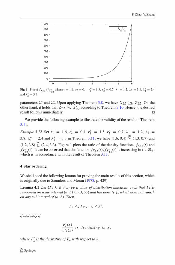
Fig. 1 Plot of fX2:2/ fX∗2:2 when r1 = 1.6, r2 = 0.4, r∗

1 = 1.3, r∗2 = 0.7, λ1 = 1.2, λ2 = 3.8, λ∗

1 = 2.4

and λ∗2 = 3.3

parameters λ∗1 and λ∗

2. Upon applying Theorem 3.8, we have X2:2 ≥lr Z2:2. On theother hand, it holds that Z2:2 ≥lr X∗

2:2 according to Theorem 3.10. Hence, the desiredresult follows immediately. �

We provide the following example to illustrate the validity of the result in Theorem3.11.

Example 3.12 Set r1 = 1.6, r2 = 0.4, r∗1 = 1.3, r∗

2 = 0.7, λ1 = 1.2, λ2 =3.8, λ∗

1 = 2.4 and λ∗2 = 3.3 in Theorem 3.11, we have (1.6, 0.4)

m� (1.3, 0.7) and

(1.2, 3.8)w� (2.4, 3.3). Figure 1 plots the ratio of the density functions fX2:2(t) and

fX∗2:2(t). It can be observed that the function fX2:2(t)/ fX∗

2:2(t) is increasing in t ∈ �+,which is in accordance with the result of Theorem 3.11.

4 Star ordering

We shall need the following lemma for proving the main results of this section, whichis originally due to Saunders and Moran (1978, p. 429).

Lemma 4.1 Let {Fλ|λ ∈ �+} be a class of distribution functions, such that Fλ issupported on some interval (a, b) ⊆ (0,∞) and has density fλ which does not vanishon any subinterval of (a, b). Then,

Fλ ≤� Fλ∗ , λ ≤ λ∗,

if and only if

F ′λ(x)

x fλ(x)is decreasing in x,

where F ′λ is the derivative of Fλ with respect to λ.

123





2. Ifr1 ≥ r2, λ1 ≤ λ2 and λ∗

1 ≤ λ∗2, then

λ2

λ1≥ λ∗

2

λ∗1

�⇒ X2:2 ≥� X∗2:2.

Proof Case 1: λ1 + λ2 = λ∗1 + λ∗

2Without loss of generality, suppose that λ1 + λ2 = λ∗

1 + λ∗2 = 1. In this case, we

have

(λ1, λ2)m� (λ∗

1, λ∗2).

Denote λ = λ2 and λ∗ = λ∗2, and it is known that λ ≥ λ∗ and λ ∈ [1/2, 1). In virtue

of Lemma 4.1, it suffices to prove that

F ′λ(t)

t fλ(t)

is decreasing in t ∈ �+ for λ ∈ [1/2, 1).The distribution function of X2:2 can be written as

Fλ(t) =t∫

0

(1 − λ)r1

�(r1)ur1−1e−(1−λ)udu

t∫

0

λr2

�(r2)ur2−1e−λudu, t > 0

with its density function as

fλ(t) = (1 − λ)r1

�(r1)tr1−1e−(1−λ)t

t∫

0

λr2

�(r2)ur2−1e−λudu

+ λr2

�(r2)tr2−1e−λt

t∫

0

(1 − λ)r1

�(r1)ur1−1e−(1−λ)udu, t > 0.

Taking the derivative to Fλ(t) with respect to λ yields that

F ′λ(t) =

⎡⎣−r1

t∫

0

(1 − λ)r1−1

�(r1)ur1−1e−(1−λ)udu +

t∫

0

(1 − λ)r1

�(r1)ur1 e−(1−λ)udu

⎤⎦

×t∫

0

λr2


123

P. Zhao, Y. Zhang

+⎡⎣r2

t∫

0

λr2−1

�(r2)ur2−1e−λudu −

t∫

0

λr2

�(r2)ur2 e−λudu

⎤⎦

×t∫

0

(1 − λ)r1

�(r1)ur1−1e−(1−λ)udu. (14)

Upon using integration by parts, one has

r

t∫

0

λr−1

�(r)ur−1e−λudu = λr−1

�(r)tr e−λt +

t∫

0

λr

�(r)ur e−λudu,

and then (14) can be reduced to

F ′λ(t) = − (1 − λ)r1−1

�(r1)tr1e−(1−λ)t

t∫

0

λr2


+λr2−1

�(r2)tr2 e−λt

t∫

0

(1 − λ)r1

�(r1)ur1−1e−(1−λ)udu, t > 0.

Thus, we can write

F ′λ(t)

t fλ(t)=

−λtr1 e−(1−λ)t∫ t

0ur2−1e−λudu + (1 − λ)tr2 e−λt

∫ t

0ur1−1e−(1−λ)udu

λ(1 − λ)tr1 e−(1−λ)t∫ t

0ur2−1e−λudu + λ(1 − λ)tr2 e−λt

∫ t

0ur1−1e−(1−λ)udu

∝−λe(2λ−1)t

∫ 1

0yr2−1e−λyt dy + (1 − λ)

∫ 1

0yr1−1e−(1−λ)yt dy

e(2λ−1)t∫ 1

0yr2−1e−λyt dy +

∫ 1


= −λ+

∫ 1


∫ 1

0

[yr1−1e−(1−λ)yt + yr2−1e(2λ−1−λy)t

]dy

,

and it is enough to prove the function

�(t) =

∫ 1


∫ 1

0

[yr1−1e−(1−λ)yt + yr2−1e(2λ−1−λy)t

]dy

= Etκ(Y, t)

123


is decreasing in t ∈ �+ for λ ∈ [1/2, 1), and where

κ(y, t) = yr1−1e−(1−λ)yt

yr1−1e−(1−λ)yt + yr2−1e(2λ−1−λy)t

for y ∈ (0, 1). Here, the distribution function of the random variable Y belongs to thefamily P2 = {H2(·|t), t ∈ �+} with densities

h2(y|t) = c2(t)[yr1−1e−(1−λ)yt + yr2−1e(2λ−1−λy)t ]

and a normalizing constant c2(t) such that∫ 1

0 h2(y|t)dy = 1. It is easy to see that

κ(y, t) = 1

1 + yr2−r1 e(2λ−1)(1−y)t

is decreasing in t ∈ �+ while is increasing in y ∈ (0, 1). On the other hand, fort2 ≥ t1 ≥ 0 and a = r1 − r2 ≥ 0, the function

ι(y) = h(y|t2)h(y|t1)

= yr1−1e−(1−λ)t2 y + yr2−1e(2λ−1−λy)t2

yr1−1e−(1−λ)t1 y + yr2−1e(2λ−1−λy)t2

= yae−(1−λ)t2 y + e(2λ−1−λy)t2

yae−(1−λ)t1 y + e(2λ−1−λy)t1

is decreasing in y ∈ (0, 1) by noting that

ι′(y) sgn=[(

a

y− (1 − λ)t2

)yae−(1−λ)t2 y − λt2e(2λ−1−λy)t2

]

×[

yae−(1−λ)t1 y + e(2λ−1−λy)t1]

−[(

a

y− (1 − λ)t1

)yae−(1−λ)t1 y − λt1e(2λ−1−λy)t1

]

×[

yae−(1−λ)t2 y + e(2λ−1−λy)t2]

= (1 − λ)(t1 − t2)y2ae−(1−λ)(t1+t2)y

+[(1 − λ)t1 − λt2 − a

y

]yae−(1−λ)t1 ye(2λ−1−λy)t2

+[

a

y− (1 − λ)t2 + λt1

]yae−(1−λ)t2 ye(2λ−1−λy)t1 (15)

+λ(t1 − t2)e(2λ−1−λy)(t1+t2)

≤ (1 − λ)(t1 − t2)y2ae−(1−λ)(t1+t2)y

123

P. Zhao, Y. Zhang

+[(1 − λ)t1 − λt2 − a

y


+[

a

y− (1 − λ)t2 + λt1


+λ(t1 − t2)e(2λ−1−λy)(t1+t2)

= (1 − λ)(t1 − t2)y2ae−(1−λ)(t1+t2)y + (t1 − t2)y

ae−(1−λ)t2 ye(2λ−1−λy)t1

+λ(t1 − t2)e(2λ−1−λy)(t1+t2) ≤ 0,

where the inequality in (15) holds due to

(1 − λ)t1 − λt2 − a

y≤ (1 − 2λ)t2 − a

y≤ 0

and

−(1 − λ)t1 y + (2λ− 1 − λy)t2 ≥ −(1 − λ)t2 y + (2λ− 1 − λy)t1.

Hence, we have H2(·|t1) ≥lr H2(·|t2), which in turn implies that H2(·|t1) ≥st H2(·|t2)whenever t2 ≥ t1. Upon using Lemma 3.1 once again, we conclude that Etκ(Y, t) isdecreasing in t ∈ (0,∞) for λ ∈ [1/2, 1), which completes the proof of this part.

Case 2: λ1 + λ2 �= λ∗1 + λ∗

2Without loss of generality, assume that λ1 + λ2 = c(λ∗

1 + λ∗2), where c is a scalar.

It then holds that

(λ1, λ2)m� (cλ∗

1, cλ∗2).

Let Y2:2 be the lifetime of a parallel system consisting of two independent gammacomponents with respective shape parameters r1 and r2 and respective scale parameterscλ∗

1 and cλ∗2. From the result of Case 1, we have

X2:2 ≥� Y2:2.

On the other hand, since the star order is scale invariant, it follows that

X2:2 ≥� X∗2:2.

�Note that the condition in Theorem 4.2 is very general which includes many special

cases (see Kochar and Xu 2011). Since the star order implies the Lorenz order, wehave the following result which is of great interest in economics.

Corollary 4.3 Let (X1, X2) be a vector of independent gamma random variableswith respective shape parameters r1 and r2 and respective scale parameters λ1 andλ2, and let (X∗



2. Ifr1 ≥ r2, λ1 ≤ λ2 and λ∗

1 ≤ λ∗2, then

123


λ2

λ1≥ λ∗

2

λ∗1

�⇒ X2:2 ≥Lorenz X∗2:2.

As an immediate consequence of Theorem 4.2, we also have the following corollary.

Corollary 4.4 Let (X1, X2) be a vector of independent gamma random variableswith respective shape parameters r1 and r2 and respective scale parameters λ1 andλ2, and let (X∗


respective shape parameters r1 and r2 and common scale parameter λ. If r1 ≥ r2 andλ1 ≤ λ2, then

X2:2 ≥� X∗2:2.

Finally, we present a result for the dispersive order.




2.Suppose r2 ≤ r1 and λ1 ≤ λ∗

1 ≤ λ∗2 ≤ λ2. Then,

(λ1, λ2)w� (λ∗

1, λ∗2) �⇒ X2:2 ≥disp X∗

2:2.

Proof From Theorem 3.8, it follows that

(λ1, λ2)w� (λ∗

1, λ∗2) �⇒ X2:2 ≥lr X∗

2:2 �⇒ X2:2 ≥st X∗2:2.

Since the assumption satisfies the condition in Theorem 4.2, we have

X2:2 ≥� X∗2:2.

On the other hand, for two continuous random X and Y , if X ≤� Y , then X ≤st Y �⇒X ≤disp Y (see Ahmed et al. 1986). We now can conclude that

X2:2 ≥disp X∗2:2.

�

5 Discussion and concluding remarks

Let X1, X2 be independent gamma random variables with Xi having shape parameterri and scale parameter λi , i = 1, 2, and X∗

1, X∗2 be another set of independent gamma

random variables with X∗i having shape parameter r∗

i and scale parameter λ∗i , i = 1, 2.

Suppose r1 ≥ r2, r∗1 ≥ r∗

2 and λ1 ≤ λ∗1 ≤ λ∗

2 ≤ λ2. It is showed that

(r1, r2)m� (r∗

1 , r∗2 ), (λ1, λ2)

w� (λ∗1, λ

∗2) �⇒ X2:2 ≥lr X∗

2:2.

123

P. Zhao, Y. Zhang

It is also proved that, if r1 ≥ r2, λ1 ≤ λ2 and λ∗1 ≤ λ∗

2, then

λ2

λ1≥ λ∗

2

λ∗1

�⇒ X2:2 ≥� X∗2:2.

With the help of these two results above, it is showed, if r2 ≤ r1 and λ1 ≤ λ∗1 ≤ λ∗

2 ≤λ2, then,

(λ1, λ2)w� (λ∗

1, λ∗2) �⇒ X2:2 ≥disp X∗

2:2.

These results have generalized and extended the results for the exponential case andthe results for the special case when having same shape parameters established earlier.Along the line of likelihood ratio order handled in the above result, it would also be ofinterest to check whether, under the condition r1 ≥ r2, r∗

1 ≥ r∗2 and λ1 ≤ λ∗

1 ≤ λ∗2 ≤

λ2,

(r1, r2)m� (r∗

1 , r∗2 ), (λ1, λ2)

p� (λ∗1, λ

∗2) �⇒ X2:2 ≥hr X∗

2:2 (16)

and

(r1, r2)m� (r∗

1 , r∗2 ), (λ1, λ2)

rm� (λ∗1, λ

∗2) �⇒ X2:2 ≥mrl X∗

2:2

hold. These remain open. We are currently working on these problems and hope toreport these findings in a future paper. The following example supports the conjecturein (16).

Example 5.1 Set r1 = 0.8, r2 = 0.5, r∗1 = 0.7, r∗

2 = 0.6, λ1 = 2, λ2 = 4, λ∗1 =

2.8 and λ∗2 = 3.4, we have (0.8, 0.5)

m� (0.7, 0.6) and (2, 4)p� (2.8, 3.4). Figure 2

0 0.5 1 1.5 2 2.5 3 3.5 4 4.5 51

1.5

2

2.5

3

3.5

hX

2:2

(t)

hX

*

2:2

(t)

Fig. 2 Plot of the hazard rate functions h X2:2 (t) and h X∗2:2 (t) when r1 = 0.8, r2 = 0.5, r∗

1 = 0.7, r∗2 =

0.6, λ1 = 2, λ2 = 4, λ∗1 = 2.8 and λ∗

2 = 3.4

123


plots the hazard rate functions h X2:2(t) and h X∗2:2(t). It can be seen that the function

h X2:2(t) is always smaller than h X∗2:2(t) in t ∈ �+.

Acknowledgments The authors would like to thank two anonymous reviewers for their valuable com-ments and suggestions on an earlier version of this manuscript which resulted in this improved version.

Appendix

Proof of Lemma 3.3 Upon using integration by parts, one gets

r

t∫

0

ur−1e−λudu = tr e−λt + λ

t∫

0

ur e−λudu.

It follows that

g(r) =r∫ t

0ur−1e−λudu − tr e−λt

∫ t

0ur−1e−λudu

=λ

∫ t

0ur e−λudu

∫ t

0ur−1e−λudu

is increasing in r ∈ �+ by a simple application of Lemma 3.1. �Proof of Lemma 3.4 According to the assumption, we have 0 < λ1 ≤ λ∗

1 ≤ λ∗2 ≤ λ2

and λ1 + λ2 = λ∗1 + λ∗

2. We first prove that, for each fixed y ∈ (0, 1), the functionϕ(y, t) is increasing in t ∈ �+ and, it suffices to prove that, forω ∈ (0, 1], the function

ϕ1(t) = e−λ1t + ωe−λ2t

e−λ∗1t + ωe−λ∗

2t

is increasing in t ∈ �+. Taking the the derivative of ϕ1(t) with respect to t gives riseto

ϕ′1(t)

sgn= (−λ1e−λ1t − ωλ2e−λ2t) ×(

e−λ∗1t + ωe−λ∗

2 t)

+(λ∗

1e−λ∗1 t + ωλ∗

2e−λ∗2 t)

× (e−λ1t + ωe−λ2t)

= (λ∗1 − λ1)e

−(λ1+λ∗1)t + ω(λ∗

1 − λ2)e−(λ∗

1+λ2)t

+ω(λ∗2 − λ1)e

−(λ1+λ∗2)t + ω2(λ∗

2 − λ2)e−(λ2+λ∗

2)t

≥ (λ∗1 − λ1)e

−(λ1+λ∗1)t + ω(λ∗

1 − λ2)e−(λ∗

1+λ2)t

+ω(λ∗2 − λ1)e

−(λ∗1+λ2)t + (λ∗

2 − λ2)e−(λ2+λ∗

2)t

123

P. Zhao, Y. Zhang

≥ (λ∗1 + λ∗

2 − λ1 − λ2)e−(λ2+λ∗

2)t + ω(λ∗1 + λ∗

2 − λ1 − λ2)e−(λ∗

1+λ2)t = 0,

which implies that ϕ1(t) is increasing in t ∈ �+, and thus the desired result follows.We next prove that, for each fixed t ∈ �+, the function ϕ(y, t) is also increasing

in y ∈ (0, 1), which is actually equivalent to showing that the function

ϕ2(y) = e−λ1 y + (1 − y)ae−λ2 y

e−λ∗1 y + (1 − y)ae−λ∗

2 y

is increasing in y ∈ (0, 1). Notice that

ϕ′2(y)

sgn=[λ∗

1e−λ∗1 y +

(a

1 − y+ λ∗

2

)(1 − y)ae−λ∗

2 y]

× [e−λ1 y + (1 − y)ae−λ2 y]

−[λ1e−λ1 y +

(a

1 − y+ λ2

)(1 − y)ae−λ2 y

]

×[e−λ∗

1 y + (1 − y)ae−λ∗2 y

]

= (λ∗1 − λ1)e

−(λ1+λ∗1)y +

(λ∗

1 − λ2 − a

1 − y

)(1 − y)ae−(λ∗

1+λ2)y

+(λ∗

2 − λ1 + a

1 − y

)(1 − y)ae−(λ1+λ∗

2)y

+(λ∗2 − λ2)(1 − y)2ae−(λ2+λ∗

2)y

≥ (λ∗1 − λ1)e

−(λ1+λ∗1)y +

(λ∗

1 − λ2 − a

1 − y

)(1 − y)ae−(λ∗

1+λ2)y

+(λ∗

2 − λ1 + a

1 − y

)(1 − y)ae−(λ∗

1+λ2)y + (λ∗2 − λ2)e

−(λ2+λ∗2)y

≥ (λ∗1 + λ∗

2 − λ1 − λ2)e−(λ2+λ∗

2)y + (λ∗1

+λ∗2 − λ1 − λ2)(1 − y)ae−(λ∗

1+λ2)y = 0,

which means that ϕ2(y) is increasing in y ∈ (0, 1), and the entire proof is completed. �

Proof of Lemma 3.5 It is known from the assumption that r2 ≤ r∗2 ≤ r∗

1 ≤ r1 andr1 + r2 = r∗

1 + r∗2 . Taking the the derivative of ζ(y, t) with respect to t gives rise to

∂

∂tζ(y, t)

sgn= b(1 − y)yr2 eb(1−y)t[

yr∗2 eb(1−y)t + yr∗

1

]

− b(1 − y)yr∗2 eb(1−y)t

[yr2 eb(1−y)t + yr1

]sgn= yr∗

1 +r2 − yr1+r∗2

sgn= r1 + r∗2 − r∗

1 − r2 ≥ 0,

123


which implies that ζ(y, t) is increasing in t ∈ �+. On the other hand, it is easy tocheck that, for fixed t > 0,

∂

∂yζ(y, t)

sgn=[r2 yr2−1ebt (1−y) − btyr2 ebt (1−y) + r1 yr1−1

]×

[yr∗

2 eb(1−y)t + yr∗1

]

−[r∗

2 yr∗2 −1ebt (1−y) − btyr∗

2 ebt (1−y) + r∗1 yr∗

1 −1]

×[

yr2 eb(1−y)t + yr1]

= (r2 − r∗2 )y

r2+r∗2 −1e2bt (1−y) + (r2 − bty − r∗

1 )yr∗

1 +r2−1ebt (1−y)

+(r1 + bty − r∗2 )y

r1+r∗2 −1ebt (1−y) + (r1 − r∗

1 )yr1+r∗

1 −1

≤ (r1 + r2 − r∗1 − r∗

2 )yr2+r∗

2 −1 + (r1 + r2 − r∗1 − r∗

2 )yr∗

1 +r2−1ebt (1−y)

= 0,

which implies that ζ(y, t) is decreasing in y ∈ (0, 1). �

References

Ahmed AN, Alzaid A, Bartoszewicz J, Kochar SC (1986) Dispersive and superadditive ordering. Adv ApplProbab 18:1019–1022

Balakrishnan N (2007) Permanents, order statistics, outliers, and robustness. Revista Matemática Com-plutense 20:7–107

Balakrishnan N, Rao CR (1998a) Handbook of statistics. Order statistics: theory and methods, vol 16.Elsevier, Amsterdam

Balakrishnan N, Rao CR (1998b) Handbook of statistics. Order statistics: applications, vol 17. Elsevier,Amsterdam

Barlow RE, Proschan F (1975) Statistical theory of reliability and life testing: probability models. To BeginWith, Silver Spring

Boland PJ, EL-Neweihi E, Proschan F (1994) Applications of the hazard rate ordering in reliability andorder statistics. J Appl Probab 31:180–192

Bon JL, Paltanea E (1999) Ordering properties of convolutions of exponential random variables. LifetimeData Anal 5:185–192

Bon JL, Paltanea E (2006) Comparisons of order statistics in a random sequence to the same statistics withi.i.d. variables. ESAIM Probab Stat 10:1–10

David HA, Nagaraja HN (2003) Order statistics, 3rd edn. Wiley, HobokenDykstra R, Kochar SC, Rojo J (1997) Stochastic comparisons of parallel systems of heterogeneous expo-

nential components. J Stat Plan Inference 65:203–211Joo S, Mi J (2010) Some properties of hazard rate functions of systems with two components. J Stat Plan

Inference 140:444–453Khaledi B-E, Kochar SC (2000) Some new results on stochastic comparisons of parallel systems. J Appl

Probab 37:283–291Khaledi B-E, Farsinezhad S, Kochar SC (2011) Stochastic comparisons of order statistics in the scale

models. J Stat Plan Inference 141:276–286Kochar SC, Rojo J (1996) Some new results on stochastic comparisons of spacings from heterogeneous

exponential distributions. J Multivar Anal 59:272–281Kochar SC, Xu M (2007) Stochastic comparisons of parallel systems when components have proportional

hazard rates. Probab Eng Inf Sci 21:597–609Kochar SC, Xu M (2011) On the skewness of order statistics in the mutiple-outlier models. J Appl Probab

48:271–284Mao T, Hu T (2010) Equivalent characteriztions on orderings of order statistics and sample ranges. Probab

Eng Inf Sci 24:245–262Marshall AW, Olkin I (2007) Life distributions. Springer, New YorkMarshall AW, Olkin I, Arnold BC (2011) Inequalities: theory of majorization and its applications, 2nd edn.

Springer, New York

123

P. Zhao, Y. Zhang

Misra N, van der Meulen EC (2003) On stochastic properties of m-spacings. J Stat Plan Inference 115:683–697

Müller A, Stoyan D (2002) Comparison methods for stochastic models and risks. Wiley, New YorkPaltanea E (2008) On the comparison in hazard rate ordering of fail–safe systems. J Stat Plan Inference

138:1993–1997Pledger P, Proschan F (1971) Comparisons of order statistics and of spacings from heterogeneous distrib-

utions. In: Rustagi JS (ed) Optimizing methods in statistics. Academic Press, New York, pp 89–113Proschan F, Sethuraman J (1976) Stochastic comparisons of order statistics from heterogeneous populations,

with applications in reliability. J Multivar Anal 6:608–616Saunders IW, Moran PA (1978) On the quantiles of the gamma and F distributions. J Appl Probab 15:

426–432Shaked M, Shanthikumar JG (2007) Stochastic orders. Springer, New YorkZhao P (2011) On parallel systems with heterogeneous gamma components. Probab Eng Inf Sci 25:369–391Zhao P, Balakrishnan N (2009a) Characterization of MRL order of fail–safe systems with heterogeneous

exponentially distributed components. J Stat Plan Inf 139:3027–3037Zhao P, Balakrishnan N (2009b) Mean residual life order of convolutions of heterogeneous exponential

random variables. J Multivar Anal 100:1792–1801Zhao P, Balakrishnan N (2011a) Some characterization results for parallel systems with two heterogeneous

exponential components. Statistics 45:593–604Zhao P, Balakrishnan N (2011b) New results on comparisons of parallel systems with heterogeneous gamma

components. Stat Probab Lett 81:36–44Zhao P, Li X, Balakrishnan N (2009) Likelihood ratio order of the second order statistic from independent

heterogeneous exponential random variables. J Multivar Anal 100:952–962

123

on the maxima of heterogeneous gamma variables with different shape and scale parameters

Documents