on the limit set of root systems of coxeter groups acting on lorentzian spaces
TRANSCRIPT

ON THE LIMIT SET OF ROOT SYSTEMS
OF COXETER GROUPS ACTING ON LORENTZIAN SPACES
CHRISTOPHE HOHLWEG, JEAN-PHILIPPE PREAUX, AND VIVIEN RIPOLL
Abstract. The notion of limit roots of a Coxeter group W was recently in-
troduced: they are the accumulation points of directions of roots of a root
system for W . In the case where the root system lives in a Lorentzian spaceW admits a faithful representation as a discrete reflection group of isometries
on a hyperbolic space; the accumulation set of any of its orbits is then classi-
cally called the limit set of W . In this article we show that the limit roots ofa Coxeter group W acting on a Lorentzian space is equal to the limit set of
W seen as a discrete reflection group of hyperbolic isometries. We aim for this
article to be as self-contained as possible in order to be accessible to the com-munity familiar with reflection groups and root systems and to the community
familiar with discrete subgroups of isometries in hyperbolic geometry.
1. Introduction
Coxeter groups acting on a Euclidean vector space as a linear reflection group areprecisely finite reflection groups [Bou68, Hum90]. In this case, the relation betweenreflection hyperplanes and the set of their normal vectors called root system is wellunderstood and their interplay is the main tool to study those groups. Surprisingly,the duality roots/reflection hyperplanes is not very well exploited to study othercases of Coxeter groups. That is the case for instance for Coxeter groups seenas discrete groups generated by reflections on hyperbolic spaces. This article wasmotivated by the recent series of papers [HLR11, DHR13] in which some examplesof the limit roots associated to a Coxeter group, acting as a discrete reflectiongroups on a Lorentzian space, looked like the limit set of a Kleinian group; see forinstance the Apollonian circles in Figure 1 obtained as limit set of a root system.
On one hand, any Coxeter group W has a representation as a discrete reflectionsubgroup of the orthogonal group OB(V ), where V is a finite dimensional vectorspace and B is a symmetric bilinear form. With such a representation of W arisesa natural set of vectors Φ called a root system, which are unit B-normal vectors ofthe reflection hyperplanes associated to reflections in W . The root system Φ has an
empty set of accumulation points, but the projective version Φ of Φ, represented onan affine hyperplane H, has an interesting set of accumulation points E(Φ) (see forinstance Figure 1). The set E(Φ) is called the set of limit roots of Φ and its studywas initiated in [HLR11] and continued in [DHR13]. Among other properties, it was
Date: July 31, 2013.Key words and phrases. Root system, Coxeter group, limit roots, limit set of discrete group,
Lorentzian space, discrete reflection group, Apollonian gasket, hyperbolic Coxeter group, hyper-
bolic isometries, Kleinian groups.The first author is supported by a NSERC grant and the third author is supported by a
postdoctoral fellowship from LaCIM. This collaboration was also made possible with the support
of the UMI CNRS-CRM.
1
arX
iv:1
305.
0052
v2 [
mat
h.G
R]
30
Jul 2
013
2 C. HOHLWEG, J.-P. PREAUX, AND V. RIPOLL
sβ sα∞
sδ
∞ ∞
sγ
∞ ∞
∞
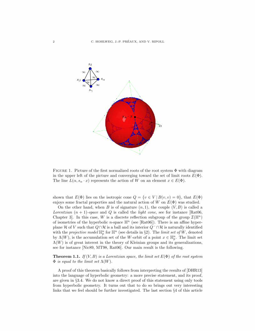
Figure 1. Picture of the first normalized roots of the root system Φ with diagramin the upper left of the picture and converging toward the set of limit roots E(Φ).The line L(α, sα · x) represents the action of W on an element x ∈ E(Φ).
shown that E(Φ) lies on the isotropic cone Q = {v ∈ V |B(v, v) = 0}, that E(Φ)enjoys some fractal properties and the natural action of W on E(Φ) was studied.
On the other hand, when B is of signature (n, 1), the couple (V,B) is called aLorentzian (n + 1)-space and Q is called the light cone, see for instance [Rat06,Chapter 3]. In this case, W is a discrete reflection subgroup of the group I(Hn)of isometries of the hyperbolic n-space Hn (see [Rat06]). There is an affine hyper-plane H of V such that Q∩H is a ball and its interior Q−∩H is naturally identifiedwith the projective model Hnp for Hn (see details in §2). The limit set of W , denotedby Λ(W ), is the accumulation set of the W -orbit of a point x ∈ Hnp . The limit setΛ(W ) is of great interest in the theory of Kleinian groups and its generalizations,see for instance [Nic89, MT98, Rat06]. Our main result is the following.
Theorem 1.1. If (V,B) is a Lorentzian space, the limit set E(Φ) of the root systemΦ is equal to the limit set Λ(W ).
A proof of this theorem basically follows from interpreting the results of [DHR13]into the language of hyperbolic geometry: a more precise statement, and its proof,are given in §3.4. We do not know a direct proof of this statement using only toolsfrom hyperbolic geometry. It turns out that to do so brings out very interestinglinks that we feel should be further investigated. The last section §4 of this article

LIMIT SET OF ROOT SYSTEMS OF COXETER GROUPS ON LORENTZIAN SPACES 3
is devoted to describe precisely the example in Figure 1 together with its relationwith Apollonian gaskets.
We aim for this article to be accessible to the community familiar with reflectiongroups and root system and to the community familiar with discrete subgroups ofisometries in hyperbolic geometry, so we will make a point to properly survey theobjects and constructions mentioned above. In particular, in §3.5.1, we discuss andmake precise the different occurrences of the word ‘hyperbolic’ in the context ofCoxeter groups.
Acknowledgments. The authors wish to thank Jean-Philippe Labbe who madethe first version of the Sage and TikZ functions used to compute and draw thenormalized roots. The second author wishes to thank Pierre de la Harpe for hisinvitation to come to Geneva in June 2013 and for his comments on this article.The third author is grateful to Pierre Py for fruitful discussions in Strasbourg inNovember 2012. We also acknowledge the participation of Nadia Lafreniere andJonathan Durand Burcombe to a LaCIM undergrad summer research award onthis theme during the summer 2012.
2. Lorentzian and hyperbolic spaces
The aim of this section is to survey the background we need on hyperbolic geom-etry. The presentation of the materials in this section is mostly based on [Rat06,Chapter 3 and §6.1], see also [BP92, Chapter A], [AVS93] and [Dav08, Chapter 6].
Let V be a real vector space of dimension n + 1 equipped with a symmetricbilinear form B. We will denote by q(·) = B(·, ·) the quadratic form associatedto B and by Q := {x ∈ V | q(x) = 0} the isotropic cone of B, or equivalently, of q.
2.1. Lorentzian spaces. Suppose from now on that the signature of B is (n, 1).The couple (V,B) is then called a Lorentzian (n+ 1)-space and Q is called the lightcone. Moreover, the elements in the set Q− := {v ∈ V | q(v) < 0} are said to betime-like, while the elements in Q+ := {v ∈ V | q(v) > 0} are space-like1; see thetop picture in Figure 2 for an illustration.
A Lorentzian transformation2 is a map on V that preserves B. So, in particular,a Lorentz transformation preserves Q, Q+ and Q−. It turns out that Lorentziantransformations are linear isomorphisms on V (by the Mazur-Ulam theorem). Wedenote by OB(V ) the set of Lorentzian transformations of V :
OB(V ) := {f ∈ GL(V ) |B(f(u), f(v)) = B(u, v), ∀u, v ∈ V }.
The well-known Cartan-Dieudonne Theorem states that, since B is non-degenerate,an element of OB(V ) is a product of at most (n+1) B-reflections: for a non-isotropicvector α ∈ V \ Q, the B-reflection associated to α (or simply reflection since B isclear) is defined by the equation3
(1) sα(v) = v − 2B(α, v)
B(α, α)α, for any v ∈ V.
1This vocabulary is borrowed from the theory of relativity, where n = 4.2Lorentzian transformations are called B-isometries in [HLR11, DHR13], since in these articles
B does not have necessarily (n, 1) for signature.3Observe that if B was a scalar product, this equation would be the usual formula for an
Euclidean reflection.

4 C. HOHLWEG, J.-P. PREAUX, AND V. RIPOLL
We denote by Hα := {v ∈ V |B(α, v) = 0} the orthogonal of the line Rα for theform B. Since B(α, α) 6= 0, we have Hα ⊕ Rα = V . It is straightforward to checkthat sα fixes Hα pointwise and that sα(α) = −α.
2.2. Hyperbolic spaces. We fix a basis B = (e1, . . . , en+1) of V such that q(v) =x2
1 + x22 + . . . x2
n − x2n+1, for any v ∈ V with coordinates (x1, . . . , xn+1) in the
basis B. With this basis, V is often denoted by Rn,1. The quadratic hyper-surface{v ∈ V | q(v) = −1}, called the hyperboloid, consists in time-like vectors and hastwo sheets. It is interesting to note that it is a differentiable surface (as the preimageof a regular value by the differentiable map q : V −→ R) and is naturally endowedwith a Riemannian metric because B(., .) restricted to the tangent spaces of eachsheet is definite positive. A vector v is positive if xn+1 > 0; the positive sheet,
Hn := {v ∈ V | q(v) = −1 and xn+1 > 0}
turns out to be a simply connected complete Riemannian manifold with constantsectional curvature equal to −1 (cf. [BP92, Theorem A.6.7]). This is the hyperboloidmodel of the hyperbolic n-space, see Figure 2. The distance function d on Hn satisfiesthe equation cosh d(x, y) = −B(x, y).
2.2.1. Group of isometries. Observe that the group OB(V ) acts on the quadratichyper-surface {v ∈ V | q(v) = −1}. A Lorentz transformation is a positive Lorentztransformation if it maps time-like positive vectors to time-like positive vectors. Sothe group O+
B(V ) of positive Lorentz transformations preserves Hn and its distance,
and the group of isometries I(Hn) of Hn is isomorphic to O+B(V ): any isometry
of Hn is the restriction to Hn of a positive Lorentz transformation. Moreover, itis well known that I(Hn) is generated by hyperbolic reflections across hyperbolichyperplanes, of which we now recall the definition.
2.2.2. Hyperbolic reflections. A linear subspace F of V is said to be time-like ifF ∩Q− 6= ∅, otherwise it is space-like. An hyperbolic hyperplane is the intersectionof Hn with a time-like hyperplane of V . Let H be a linear hyperplane in V andα ∈ V be a normal vector to H for the form B. Since H ⊕ Rα = V , we havenecessarily that H is time-like if and only if α ∈ V is a space-like vector. Areflection sα ∈ OB(V ) is an hyperbolic reflection if α⊥ = H is a time-like hyperplaneor, equivalently, if α is a space-like vector of V . In this case, sα ∈ O+
B(V ) and itrestricts to an isometry of Hn.
Remark 2.1. The fact that sα ∈ O+B(V ) for a space-like vector α follows from
the fact that a reflection sα is continuous and that it exchanges the two sheets (i.e.connected components) of the quadratic surface {v ∈ V | q(v) = −1} if and only ifHα is space-like, i.e., if and only if α is a time-like vector.
2.3. The projective model. To make clear the link between hyperbolic geometryand the results of [HLR11, DHR13], we need to introduce another model for Hn.Consider the unit open (Euclidean) n-ball embedded in the affine hyperplane Rn×{1} of V :
Dn1 = {v ∈ V |xn+1 = 1 and x2
1 + · · ·+ x2n < 1}
and the map p from Dn1 to Hn, called the radial projection
p : Dn1 → Hn

LIMIT SET OF ROOT SYSTEMS OF COXETER GROUPS ON LORENTZIAN SPACES 5
where p(v) is the intersection point of the line Rv with Hn (see Figure 2). A simplecalculation shows that
p(v) =v√|q(v)|
.
The unit ball Dn1 endowed with the pullback metric with respect to p, i.e. which
makes p an isometry, is a (non conformal) model Hnp for Hn called the projective
ball model4, see [Rat06, §6.1].First, observe that using the equation for q in the basis B, we have that Dn
1 ⊆ Q−.Let H be the affine hyperplane directed by span(e1, . . . , en) and passing throughthe point en+1, then we get
Dn1 = Q− ∩H,
with boundary Q ∩ H. The next proposition follows from the previous discussionand [Rat06, Equation (6.1.2)].
Proposition 2.2. The projective model Hnp has underlying space Dn1 = Q− ∩ H
and its boundary ∂Hnp is Q ∩ H. Moreover, p : Hnp → Hn is an isometry whoseinverse is
p−1(v) =v
xn+1= (x1/xn+1, . . . , xn/xn+1, 1).
This proposition is illustrated for n+ 1 = 2 and n+ 1 = 3 in Figure 2.
2.3.1. Hyperplanes, reflections and isometries. The projective model gives us aneasy description of hyperplanes: an hyperbolic hyperplane in Hnp is simply the in-tersection of a time-like linear hyperplane of V with Hnp . Let I(Hnp ) be the groupof isometries of Hnp .
Corollary 2.3. The conjugation by p is an isomorphism from I(Hn) to I(Hnp ): for
ϕ ∈ I(Hn) and a point v ∈ Hnp , ϕ · v := p−1 ◦ ϕ ◦ p(v) defines the isometric actionof ϕ on Hnp . Moreover ϕ · v is the intersection point of the linear line Rϕ(v) withthe ball Dn
1 .In particular, if α ∈ V is a space-like vector, then sα · v = p−1 ◦ sα ◦ p(v) is the
hyperbolic reflection in I(Hnp ) of v across the time-like hyperplane α⊥.
Proof. This result follows immediately from Proposition 2.2” Let us detail the“moreover part”. Let (x1, . . . , xn+1) be the coordinates of v, and (y1, . . . , yn+1)the coordinates of ϕ(v), in the basis B. Since v ∈ Dn
1 and ϕ ∈ O+B(V ), we have that
xn+1 = 1 and yn+1 > 0. Therefore, ϕ(v) ∈ Q− and ϕ(v)/yn+1 ∈ Q− ∩ H = Dn1 is
the intersection point of Rϕ(v) with the ball Dn1 . Now remember the formula for
p−1 in Proposition 2.2: we have
ϕ · v = p−1 ◦ ϕ ◦ p(v) = p−1 ◦ ϕ
(v√|q(v)|
)
= p−1
(1√|q(v)|
ϕ(v)
)= p−1(ϕ(v)) =
ϕ(v)
yn+1.
�
4This model is also sometimes called the Beltrami-Klein model in the literature.
6 C. HOHLWEG, J.-P. PREAUX, AND V. RIPOLL
p(v)
Q+
Q−
Q
ve2
H1
n + 1 = 2
H1p
p(v)
H2p
n + 1 = 3
v
Q
H2
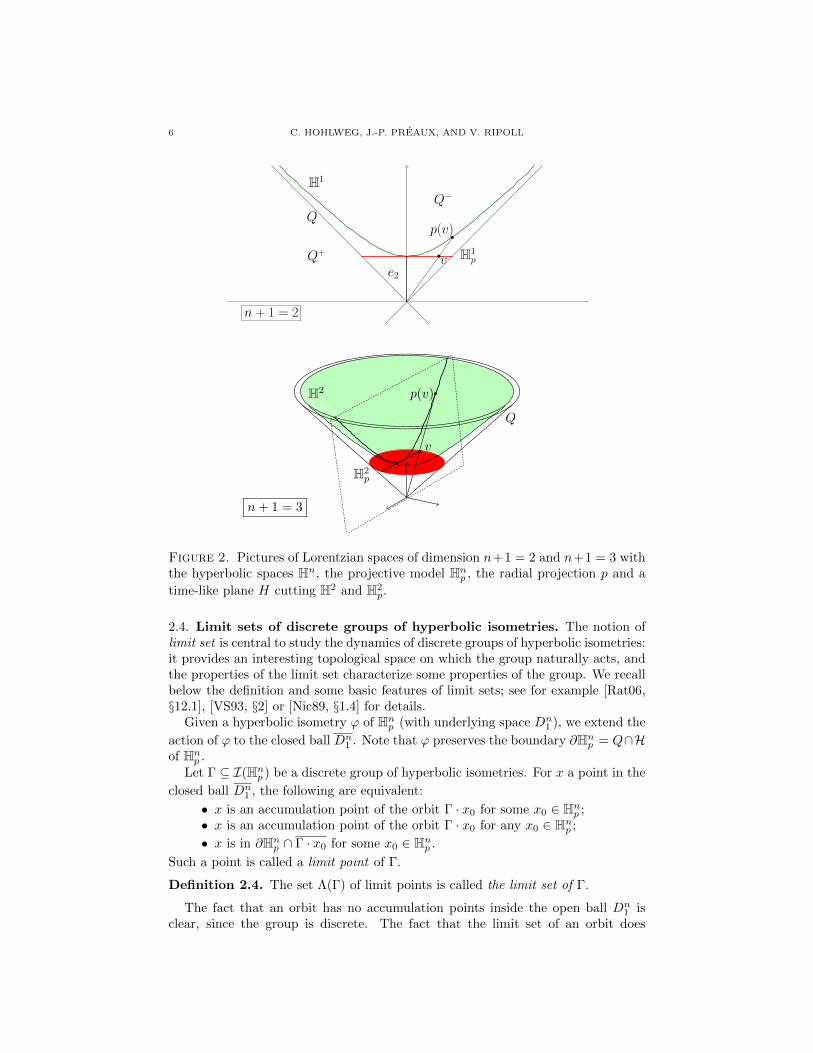
Figure 2. Pictures of Lorentzian spaces of dimension n+1 = 2 and n+1 = 3 withthe hyperbolic spaces Hn, the projective model Hnp , the radial projection p and a
time-like plane H cutting H2 and H2p.
2.4. Limit sets of discrete groups of hyperbolic isometries. The notion oflimit set is central to study the dynamics of discrete groups of hyperbolic isometries:it provides an interesting topological space on which the group naturally acts, andthe properties of the limit set characterize some properties of the group. We recallbelow the definition and some basic features of limit sets; see for example [Rat06,§12.1], [VS93, §2] or [Nic89, §1.4] for details.
Given a hyperbolic isometry ϕ of Hnp (with underlying space Dn1 ), we extend the
action of ϕ to the closed ball Dn1 . Note that ϕ preserves the boundary ∂Hnp = Q∩H
of Hnp .Let Γ ⊆ I(Hnp ) be a discrete group of hyperbolic isometries. For x a point in the
closed ball Dn1 , the following are equivalent:
• x is an accumulation point of the orbit Γ · x0 for some x0 ∈ Hnp ;• x is an accumulation point of the orbit Γ · x0 for any x0 ∈ Hnp ;
• x is in ∂Hnp ∩ Γ · x0 for some x0 ∈ Hnp .
Such a point is called a limit point of Γ.
Definition 2.4. The set Λ(Γ) of limit points is called the limit set of Γ.
The fact that an orbit has no accumulation points inside the open ball Dn1 is
clear, since the group is discrete. The fact that the limit set of an orbit does

LIMIT SET OF ROOT SYSTEMS OF COXETER GROUPS ON LORENTZIAN SPACES 7
not depend on the chosen point follows from the relation between hyperbolic andEuclidean distances, see [Rat06, Theorem 12.1.2].
The limit set Λ(Γ) is clearly closed and Γ-stable. Many general properties areknown for limit sets of discrete groups of hyperbolic isometries. For example, eitherΛ(Γ) is finite, in which case |Λ(Γ)| ≤ 2 and Γ has a finite orbit in the closed ballDn
1 , see [Rat06, Theorem 12.2.1], or Λ(Γ) is uncountable and the action of Γ onΛ(Γ) is minimal. In [DHR13], the authors show an analogous property for the setof limit roots of a root system, which we will define below.
3. Coxeter groups and hyperbolic geometry
The aim of this section is to present constructions and results related to rootsystems, and that are taken out from [Dye12, HLR11, DHR13], into the languageof hyperbolic geometry. This naturally leads to a proof of Theorem 1.1.
Recall that a Coxeter system (W,S) is such that S ⊆ W is a set of generatorsfor the Coxeter group W , subject only to relations of the form (st)ms,t = 1, wherems,t ∈ N∗ ∪ {∞} is attached to each pair of generators s, t ∈ S, with ms,s = 1 andms,t ≥ 2 for s 6= t. We write ms,t = ∞ if the product st is of infinite order. Inthe following, we always suppose that the set of generators S is finite. If all thems,t =∞ then we say that W is a universal Coxeter group.
It turns out that any Coxeter group can be represented as a discrete reflectionsubgroup of OB(V ) for a certain pair (V,B): Coxeter groups are the discrete re-flection groups associated to based root systems [Vin71, Theorem 2] (see [Kra09, §1and Theorem 1.2.2] for a recent exposition of this result).
From now on, we fix (V,B) to be a Lorentzian (n + 1)-space. Note that mostof the results from [Dye12, HLR11, DHR13] we recall in the two next sections arevalid for arbitrary (V,B).
3.1. Based root systems and geometric representations. Let us cover thebasis on based root systems (see for instance [HLR11, §1] for more details). Asimple system ∆ is a finite subset of V such that:
(i) ∆ is positively independent: if∑α∈∆ λαα = 0 with all λα ≥ 0, then all
λα = 0;
(ii) for all α, β ∈ ∆, with α 6= β, B(α, β) ∈ ]−∞,−1] ∪ {− cos(πk
), k ∈ Z≥2};
(iii) for all α ∈ ∆, B(α, α) = 1.
Denote by S := {sα |α ∈ ∆} the set of B-reflections associated to elements in ∆.Let W be the subgroup of OB(V ) generated by S, and Φ = W (∆) be the orbitof ∆ under the action of W .
The pair (Φ,∆) is called a based root system in (V,B), for simplification we willoften use the term root system instead of based root system; Φ+ = cone(∆) ∩ Φ isits set of positive roots; its rank is the cardinality of ∆, i.e., the cardinality of S.Vinberg [Vin71, Theorem 2] shows that (W,S) is always a Coxeter system and Wis a discrete reflection group in OB(V ). Such a representation of a Coxeter groupis called a geometric representation. Conversely, it is well known that any (finitelygenerated) Coxeter group can be geometrically represented with a root system, seefor instance [Hum90, Chapter 5].

8 C. HOHLWEG, J.-P. PREAUX, AND V. RIPOLL
3.2. Representations as discrete reflection groups of hyperbolic isome-tries. A geometric representation of a Coxeter group W as a discrete subgroupof OB(V ) in a Lorentzian (n + 1)-space yields a faithful representation of W as adiscrete subgroup of isometries of Hn that is generated by hyperbolic reflections;and therefore, by conjugation by the radial projection (Corollary 2.3), it also pro-vides a faithful representation of W as a discrete subgroup of I(Hnp ) generated byreflections.
The key is to observe that W ⊆ OB(V ) is in fact a subgroup of O+B(V ), the
group of positive Lorentz transformations: from §2.2.1, we know that O+B(V ) is
isomorphic to I(Hn) by restriction to Hn.
Proposition 3.1. Let (Φ,∆) be a based root system in the Lorentzian (n + 1)-space (V,B) with associated Coxeter system (W,S). Then W ⊆ O+
B(V ) and thisgeometric action of W on the (n+ 1)-Lorentzian space preserves Hn. This yields arestricted representation of W on I(Hn) that is faithful and discrete. Consequently,the projective action5 of W on Hnp is also faithful and discrete.
Moreover, the action of W on Hn (resp. Hnp ) is generated by reflections across
the hyperbolic hyperplanes α⊥ ∩Hn (resp. α⊥ ∩Hnp ) for all α ∈ ∆.
Proof. Since ∆ is a constituted of space-like vectors, the hyperplanes α⊥ are time-like. From §2.2.2 we know therefore that sα ∈ O+
B(V ) for all α ∈ ∆. Since W is
generated by S = {sα |α ∈ ∆}, we have necessarily that W ⊆ O+B(V ). �
Remark 3.2. The relative position between two hyperbolic hyperplanes has a nicecharacterization using their“normal vectors”. Let α and β be two space-like linearlyindependent vectors such that B(α, α) = B(β, β) = 1. So we know that α⊥ and β⊥
are time-like hyperplanes; moreover, denote by Hα = α⊥ ∩Hn and Hβ = β⊥ ∩Hn,then:
(i) Hα and Hβ intersect if and only if B(α, β) ∈]−1, 1[, and in which case theirdihedral angle is arccos |B(α, β)|,
(ii) Hα and Hβ are parallel if and only if B(α, β) = ±1,(iii) Hα and Hβ are ultra-parallel if and only if |B(α, β)| > 1 and in such case
their distance in Hn is cosh−1 (|B(α, β)|).(The statement (i) follows from Theorem 3.2.6 (see also the discussion that followsin §3.2 and §6.4) of [Rat06]; the statement (ii) follows from Theorem 3.2.9 of [Rat06]and the statement (iii) from Theorems 3.2.7 and 3.2.8 of [Rat06].)
3.3. Limits of roots. From now on, we fix a based root system (Φ,∆) in theLorentzian (n+1)-space (V,B) with associated Coxeter system (W,S). We assume6
that span(∆) = V ; such a root system is infinite and called a weakly hyperbolic rootsystem.
The norm of any injective sequence of roots goes to infinity, so Φ does not haveaccumulation points (see [HLR11, Theorem 2.7]). We rather look at accumulationpoints of the directions of the roots. In order to do this, we will cut those directionsby an hyperplane transverse to Φ+, i.e. an affine hyperplane that intersects all the
5From Corollary 2.3.6Otherwise we could restrict our study to the subspace span(∆), in which Φ could be finite,
affine or weakly hyperbolic, depending of the signature of the restriction of B to this subspace,see [DHR13] for more details.

LIMIT SET OF ROOT SYSTEMS OF COXETER GROUPS ON LORENTZIAN SPACES 9
directions of the roots. So we get points that are representatives of those directions,see for instance 3.
Q−
α = ρ1β = ρ′1
ρ2ρ′2
ρ3ρ′3
ρ4ρ′4
V1
V1
α = ρ1β = ρ′1 ρ2ρ′2 · · ·
Q−
sα sβ∞(−1.01)
Figure 3. The isotropic cone Q and the first positive roots and normalizedroots of an infinite based root system of rank 2 with B(α, β) = 1, 01 in aLorentzian 2-space.
The discussion in §2 depends heavily on the basis B of §2.2. By [DHR13, Proposi-tion 4.13], we can fix B = (e1, . . . , en+1) such that H is transverse to Φ+. Moreover,B and H have the following properties:
(1) B(en+1, α) < 0 for all α ∈ ∆.(2) Denote by H the linear hyperplane directing H, and for v ∈ V \H, denote
by v the intersection point of the line Rv with H (we also use the analog
notation P for a subset P of V \H), see [HLR11, §2.1 and §5.2] for moredetails. With these notations we have:(a) Hnp = Q− = Q− ∩ H and its boundary is ∂Hnp = Q ∩ H = Q, by
Proposition 2.2;
(b) for any x ∈ Hnp and w ∈W , w · x = w(x), by Corollary 2.3.
Our main objects of study are:
• The set of normalized roots Φ := {β |β ∈ Φ}, which is contained in the
convex hull of the normalized simple roots α in ∆, seen as points in V1,the affine hyperplane xn+1 = 1. The normalized roots are representativesof the directions of the roots, or in other words, of the roots seen in theprojective space PV . In Figure 1, normalized roots are in blue, while the
edges of the polytope conv(∆) are in green.
• The set E(Φ) of accumulation points of Φ, to which tends the blue shapein Figure 1. For short, we call the elements of E(Φ), which are limit pointsof normalized roots, the limit roots of Φ.
• The action of W on conv(E(Φ)) t Φ defined by w · x = w(x), see [DHR13,§2.3]. Since the root system is weakly hyperbolic W acts faithfully on E(Φ)by [DHR13, Theorem 6.1].

10 C. HOHLWEG, J.-P. PREAUX, AND V. RIPOLL
The set E(Φ) also enjoys some fractal properties as shown in [DHR13, §4], seealso [HMN12]. It was those fractal properties that led us to exhibit the link withlimit sets of discrete groups generated by hyperbolic reflections (Theorem 1.1).
3.4. Imaginary convex set and proof of Theorem 1.1. We prove here Theo-rem 1.1 from the introduction, whose precise statement is given below.
Theorem 3.3. Let (Φ,∆) be a weakly hyperbolic root system in a Lorentzian space(V,B), and W ⊆ I(Hnp ) its associated Coxeter group. Then the limit set Λ(W )of W is equal to the set E(Φ) of limit roots of Φ.
Since to study the limit set of W we may choose any point in Hnp , see §2.4, wewill actually consider a particular subset that intersects Hnp : the imaginary convexset, see [DHR13, §2]. The imaginary convex set is the projective version of theimaginary cone that has been first introduced by Kac (see [Kac90, Ch. 5]) in thecontext of Weyl groups of Kac-Moody Lie algebras; this notion has been generalizedafterwards to arbitrary Coxeter groups, first by Hee [Hee93], then by Dyer [Dye12](see also Edgar’s thesis [Edg09] or Fu’s article [Fu11]). The definition we use hereapplies to any finitely generated Coxeter group, and is illustrated in Figure 4.
Definition 3.4. The imaginary convex set Z(Φ) is the W -orbit of the polytope
K := {v ∈ conv(∆) |B(v, α) ≤ 0, ∀α ∈ ∆}.
The imaginary convex set is intimately linked with the set of limit roots, see [DHR13,§2]:
conv(E(Φ)) = Z ⊆ {v ∈ H |B(v, v) ≤ 0} ⊆ Q−.Moreover, since (Φ,∆) is weakly hyperbolic, we know by [DHR13, Lemma 2.4] that
the polytope K has non-empty interior. In particular K and Z intersect Hnp = Q−.Therefore, W acts on the non-empty set Z ∩Hnp with the action of Corollary 2.3.
Now, the limit set of W is independent of the choice of the initial chosen pointin Hnp , see §2.4. Thus, for any v ∈ Z ∩Hnp , the limit set of W :
Λ(W ) = Acc(W · v).
Still using the assumption that (Φ,∆) is weakly hyperbolic, we have by [DHR13,Corollary 6.15(c)]:
(2) E(Φ) = Acc(W · v), for v ∈ ZThis proves Theorem 3.3 and therefore Theorem 1.1.
Remark 3.5. It is shown in [DHR13, Theorem 4.10], since the root system isweakly hyperbolic, that E(Φ) can be recovered easily from Z: E(Φ) = Z ∩Q. Thisproperty is the key to prove Equation (2). Whether these two properties are true ornot for root systems, when (V,B) is not a Lorentzian or Euclidean space, is an openquestion, see [DHR13, Question 4.9] and the proof of [DHR13, Corollary 6.15(c)].
3.5. Discrete groups generated by hyperbolic reflections and Coxetergroups. The word“hyperbolic”is often attached to the expression“Coxeter groups”in the literature. In the same vein, the relation between “discrete groups gen-erated by hyperbolic reflections” and “hyperbolic Coxeter groups” is not alwaysclearly transparent. It does not always seem to mean the same thing. For in-stance, in the article of Krammer [Kra09], “hyperbolic Coxeter group” means aCoxeter group attached to a weakly hyperbolic root system, whereas in Humphreys’

LIMIT SET OF ROOT SYSTEMS OF COXETER GROUPS ON LORENTZIAN SPACES 11
α β
γ
sα sβ-1.2
sγ
-1.2 -1.2
K
sα ·K
Figure 4. Picture in rank 3 of the first 9 normalized roots for the weakly hyperbolic
root system with diagram in the upper left of the picture. In red is Q = ∂H2p and
in green is the boundary of conv(∆). Some reflections hyperplanes for W , K andsome of its images through reflections are also represented in shaded yellow.
book [Hum90] this means a strict subclasses of Coxeter groups attached to a weaklyhyperbolic root system. See also the difference in the use of these expressions be-tween [Dav08, Rat06, AB08] or [Dol08]. We end this section by clarifying therelation between those terms.
3.5.1. Discrete reflection groups of hyperbolic isometries. A discrete reflection groupon Hn is a discrete subgroup of hyperbolic isometries Γ ⊆ I(Hn) generated by(finitely many) hyperbolic reflections, see [VS93, Chapter 5, §1.2]. We explainedbefore how a Coxeter group with a root system in a Lorentzian space has a repre-sentation as a discrete reflection group, see propositon 3.1. Conversely, we have thefollowing theorem.
Theorem 3.6 (Vinberg [Vin71, VS93]). Discrete reflection groups on Hn are Cox-eter groups that are associated to based root systems in Lorentzian spaces.
This result due to Vinberg completes for spaces of constant curvature the classicalresult of Coxeter [Cox34] that shows that: (1) discrete reflection groups on thesphere (i.e. Euclidean vector space) are finite and are Coxeter groups; (2) discretereflection groups on affine Euclidean space are Coxeter groups. Moreover, Coxeterclassified those groups in the case of the sphere and of the affine Euclidean space,see [Hum90]. Such a classification is still unknown for Coxeter groups that arise asdiscrete reflection groups on Hn. Only the subclass of hyperbolic reflection groupsis classified, see below for more details.
Remark 3.7 (Remark on the proof). To show that a discrete reflection group Γon Hn is a Coxeter group is a bit more complicated than in the case of the sphere andof the affine Euclidean space, but the main steps are the same. To our knowledge,the theorem above is never stated precisely in these terms, but is clearly apparentin [VS93, Chapter 5, §1.1 and §1.2].
12 C. HOHLWEG, J.-P. PREAUX, AND V. RIPOLL
First, consider the hyperplane arrangement associated to Γ, i.e., the set of hy-perplanes of the reflections in Γ. This hyperplane arrangement is locally finite andtherefore decomposes Hn into (hyperbolic) convex polyhedra (each of these is aDirichlet domain, see [VS93] or [Rat06, §6.6]). Pick one of these to be the funda-mental chamber7 P , which is a convex polyhedron. Then this fundamental chamberis a fundamental domain for the action of Γ on Hn and the angles between the facetsthat intersect8 are submultiples of π, see [VS93, Chapter 5, §1.1 and Proposition1.4] or [Dol08, Theorem 2.1]. Then, by [Vin71, Theorem 2], we know that theexterior unitary (for B) normal vector in V associated to the facets of P form asimple system ∆ and its orbit Φ is a root system. Finally, by denoting S the setof reflections across the facets of P , one deduces that (Γ, S) is a Coxeter systemassociated to the based root system (Φ,∆) (see also [Kra09, Theorem 1.2.2]).
3.5.2. Fundamental polyhedron of discrete reflection groups of hyperbolic isometries.Let W ⊆ I(Hn) be a discrete reflection group on Hn, with associated root system(Φ,∆) in (V,B). A fundamental convex polyhedron P , i.e., a fundamental chamberas in the remark above, can be easily described with the help of the Tits cone. SinceB is non-degenerate, we associate V and its dual. So
C := {v ∈ V |B(v, α) ≥ 0, ∀α ∈ ∆}is a fundamental domain for the action of W on the Tits cone U , which is the unionof the W -orbit W (C); we call C the fundamental chamber.
Remark 3.8. Observe that with Definition 3.4, K = (−C) ∩ conv(∆), and theimaginary convex set Z is contained in the negative of the Tits cone −U , see Fig-ure 5.
The following proposition is mostly a reinterpretation of classical results, see forinstance [Kra09].
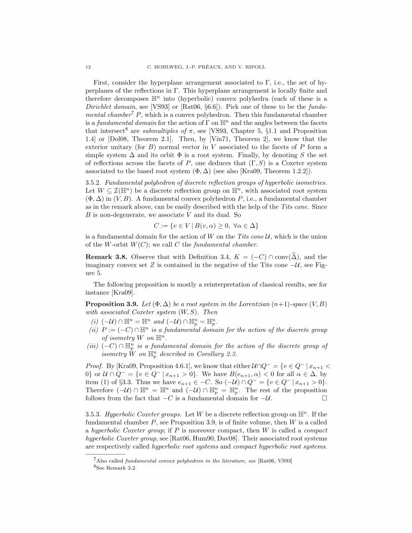
Proposition 3.9. Let (Φ,∆) be a root system in the Lorentzian (n+1)-space (V,B)with associated Coxeter system (W,S). Then
(i) (−U) ∩Hn = Hn and (−U) ∩Hnp = Hnp .(ii) P := (−C)∩Hn is a fundamental domain for the action of the discrete group
of isometry W on Hn.(iii) (−C) ∩ Hnp is a fundamental domain for the action of the discrete group of
isometry W on Hnp described in Corollary 2.3.
Proof. By [Kra09, Proposition 4.6.1], we know that either U∩Q− = {v ∈ Q− |xn+1 <0} or U ∩ Q− = {v ∈ Q− |xn+1 > 0}. We have B(en+1, α) < 0 for all α ∈ ∆, byitem (1) of §3.3. Thus we have en+1 ∈ −C. So (−U) ∩Q− = {v ∈ Q− |xn+1 > 0}.Therefore (−U) ∩ Hn = Hn and (−U) ∩ Hnp = Hnp . The rest of the propositionfollows from the fact that −C is a fundamental domain for −U . �
3.5.3. Hyperbolic Coxeter groups. Let W be a discrete reflection group on Hn. If thefundamental chamber P , see Proposition 3.9, is of finite volume, then W is a calleda hyperbolic Coxeter group; if P is moreover compact, then W is called a compacthyperbolic Coxeter group, see [Rat06, Hum90, Dav08]. Their associated root systemsare respectively called hyperbolic root systems and compact hyperbolic root systems.
7Also called fundamental convex polyhedron in the literature, see [Rat06, VS93]8See Remark 3.2.

LIMIT SET OF ROOT SYSTEMS OF COXETER GROUPS ON LORENTZIAN SPACES 13
α β
γ
sα sβ∞
sγ
∞ ∞
K
sα ·K
Figure 5. A hyperbolic root system. Picture in rank 3 of the first normalized rootconverging toward the set of limits of roots E(Φ) for the root system with diagram
in the upper left of the picture. In red is Q = ∂H2p. Reflections hyperplanes for W
and K are also represented. Note that here K ∩H2p = −C ∩H2
p is not compact but
has a finite volume in H2p, see §3.5.3.
These two classes of root systems can be characterized as strict subclasses of weaklyhyperbolic root systems, see for instance [Dye12, §9] or [DHR13, §4.1]. Let (Φ,∆)be a weakly hyperbolic root system, then
• (Φ, δ) is hyperbolic if and only if B restricts to a positive form on each proper
faces of cone(∆), i.e. −C ⊆ conv(∆); an example is given in Figure 5• (Φ,∆) is compact hyperbolic if and only if B restricts to a positive definite
form on each proper faces of cone(∆), i.e. −C ⊆ int(conv(∆)); an exampleis given in Figure 6. In particular, a compact hyperbolic Coxeter groupcannot have a relation of the form ms,t =∞.
The example in Figure 4 is neither compact hyperbolic nor hyperbolic, andK ∩H2
p ( −C ∩H2p.
Remark 3.10. We should be careful with the terminology here, because the prop-erties studied often depend on the geometry, i.e., on W as a discrete reflection groupon Hn and not only as an abstract Coxeter group.
(1) For this reason, we do not say that a Coxeter group associated to a weaklyhyperbolic root system is a“weakly hyperbolic Coxeter group”: for example,the universal Coxeter group of rank 4 admits a representation with a weaklyhyperbolic root system, but it also admits a representation with a rootsystem of signature (2, 2), which is therefore not weakly hyperbolic, see[DHR13, Remark 4.3 and Figure 5].
(2) In the case of rank 3 Coxeter groups, we should avoid using the terminology“hyperbolic Coxeter groups”. Indeed, for instance, the universal Coxetergroup of rank 3 admits a geometric representation attached to a weaklyhyperbolic, non hyperbolic, root system (see Figure 4), and a geometricrepresentation attached to a hyperbolic root system (see Figure 5). This
14 C. HOHLWEG, J.-P. PREAUX, AND V. RIPOLL
α β
γ
sα sβ4
sγ
4 4
K
sα ·K
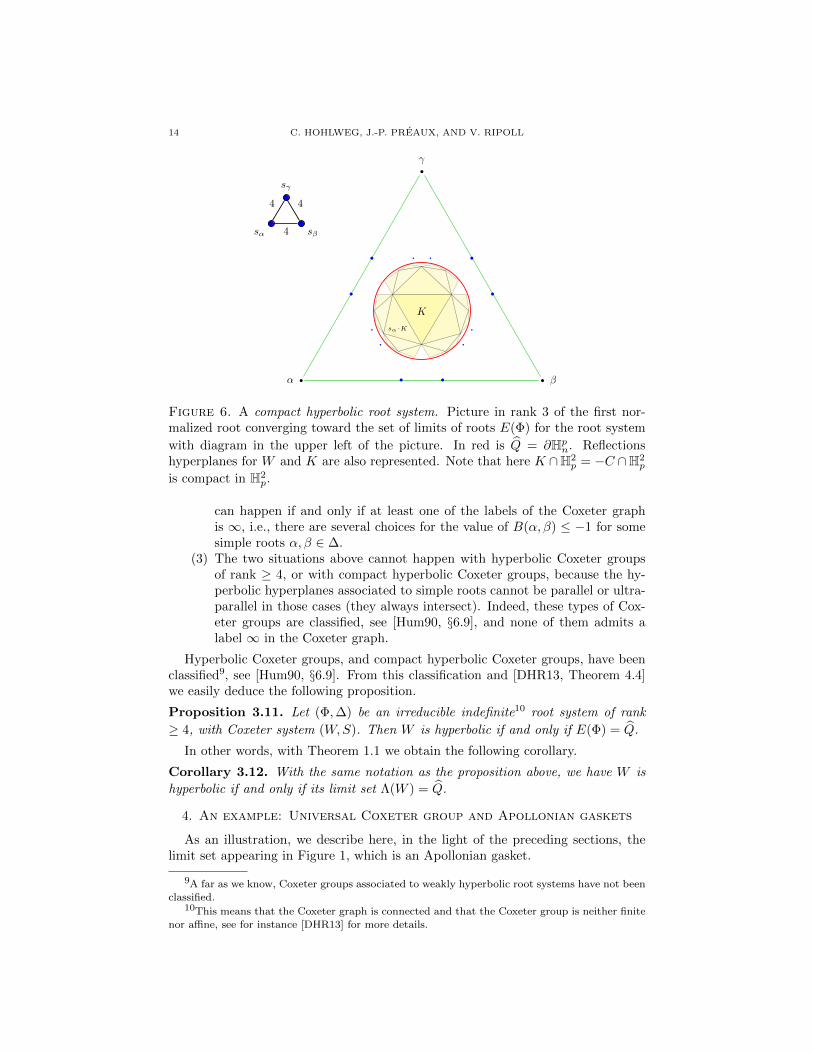
Figure 6. A compact hyperbolic root system. Picture in rank 3 of the first nor-malized root converging toward the set of limits of roots E(Φ) for the root system
with diagram in the upper left of the picture. In red is Q = ∂Hpn. Reflectionshyperplanes for W and K are also represented. Note that here K ∩H2
p = −C ∩H2p
is compact in H2p.
can happen if and only if at least one of the labels of the Coxeter graphis ∞, i.e., there are several choices for the value of B(α, β) ≤ −1 for somesimple roots α, β ∈ ∆.
(3) The two situations above cannot happen with hyperbolic Coxeter groupsof rank ≥ 4, or with compact hyperbolic Coxeter groups, because the hy-perbolic hyperplanes associated to simple roots cannot be parallel or ultra-parallel in those cases (they always intersect). Indeed, these types of Cox-eter groups are classified, see [Hum90, §6.9], and none of them admits alabel ∞ in the Coxeter graph.
Hyperbolic Coxeter groups, and compact hyperbolic Coxeter groups, have beenclassified9, see [Hum90, §6.9]. From this classification and [DHR13, Theorem 4.4]we easily deduce the following proposition.
Proposition 3.11. Let (Φ,∆) be an irreducible indefinite10 root system of rank
≥ 4, with Coxeter system (W,S). Then W is hyperbolic if and only if E(Φ) = Q.
In other words, with Theorem 1.1 we obtain the following corollary.
Corollary 3.12. With the same notation as the proposition above, we have W is
hyperbolic if and only if its limit set Λ(W ) = Q.
4. An example: Universal Coxeter group and Apollonian gaskets
As an illustration, we describe here, in the light of the preceding sections, thelimit set appearing in Figure 1, which is an Apollonian gasket.
9A far as we know, Coxeter groups associated to weakly hyperbolic root systems have not beenclassified.
10This means that the Coxeter graph is connected and that the Coxeter group is neither finitenor affine, see for instance [DHR13] for more details.

LIMIT SET OF ROOT SYSTEMS OF COXETER GROUPS ON LORENTZIAN SPACES 15
4.1. Conformal models of the hyperbolic space. We now introduce two con-formal models of the hyperbolic space, the conformal ball model and the upperhalfspace model that turn out to be more practical to deal with the geometry be-cause their isometries are Mobius transformations. For details we refer the readerto [Rat06, Chapter 4] and [BP92, Chapter A]. We use the notation ‖.‖ for theEuclidean norm of Rn.
4.1.1. Inversions and the Mobius group. In the Euclidean space Rn endowed withits standard scalar product, let S(a, r) denotes a sphere with center a and radiusr. The inversion with respect to S(a, r) is the map:
ia,r : Rn \ {a} −→ Rn \ {a}x 7−→ a+ r2. x−a
‖x−a‖2
It is an involutive diffeomorphism that is conformal and changes spheres intospheres. It extends to an involution Ia,r of the one point compactification Rn =Rn ∪ {∞} by setting Ia,r(a) = ∞ and Ia,r(∞) = a, which is a conformal invo-
lutive diffeomorphism once Rn is given its standard diffeomorphic and conformalstructures. Then Ia,r changes spheres/hyperplanes into spheres/hyperplanes. Itsset of fixed points is the whole sphere S(a, r), and conformality implies that asphere/hyperplane H is stable under Ia,r if and only if H intersects S(a, r) or-thogonally. Whenever Ia,r changes the sphere Sb,ρ into an hyperplane H thenIa,r ◦ Ib,ρ ◦ I−1
a,r is the Euclidean (orthogonal) reflection with respect to H. The
Mobius group of Rn (or Rn) is defined as the group generated by all inversions andreflections in Rn.
4.1.2. The Conformal Ball Model Hnc . Consider the open unit ball embedded in thehyperplane Rn × {0} of V :
Dn = {(x1, . . . , xn+1) ∈ V |xn+1 = 0 and x21 + · · ·+ x2
n = 1}
and the stereographic projection c with respect to −en+1 of Rn×R∗+ onto Rn×{0}:
c : Rn × R∗+ −→ Rn × {0}(x1, . . . , xn+1) 7−→ (x1,...,xn,0)
1+xn+1
One verifies that c restricted to the hyperboloid model Hn is a diffeomorphismonto Dn (cf. [Rat06, BP92]). Once Dn is endowed with the pull-back metric(the Riemannian metric ds = dx
1−‖x‖2 ) one obtains the conformal ball model of the
hyperbolic space, that we denote by Hnc (cf. Figure 7).The (hyperbolic) hyperplanes in Hnc are the intersections with Dn of the Eu-
clidean spheres and hyperplanes in Rn × {0} that are perpendicular to the bound-ary sphere ∂Hnc := ∂Dn. The hyperbolic reflection with axis the hyperplane H isthe restriction of the inversion with respect to the Euclidean sphere or hyperplanein Rn × {0} containing H. It turns out that the group of isometries I(Hnc ) is thesubgroup of the Mobius group of Rn × {0} that leaves invariant Dn or, equiva-lently, generated by inversions/reflections with respect to hyperplanes/spheres thatare perpendicular to the boundary. The model is conformal: the hyperbolic andEuclidean angles are the same.
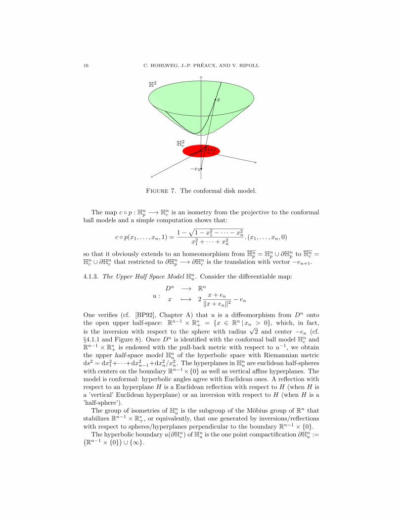
16 C. HOHLWEG, J.-P. PREAUX, AND V. RIPOLL
−e3
c(x)
x
H2c
H2
Figure 7. The conformal disk model.
The map c ◦ p : Hnp −→ Hnc is an isometry from the projective to the conformalball models and a simple computation shows that:
c ◦ p(x1, . . . , xn, 1) =1−
√1− x2
1 − · · · − x2n
x21 + · · ·+ x2
n
. (x1, . . . , xn, 0)
so that it obviously extends to an homeomorphism from Hnp = Hnp ∪ ∂Hnp to Hnc =Hnc ∪ ∂Hnc that restricted to ∂Hnp −→ ∂Hnc is the translation with vector −en+1.
4.1.3. The Upper Half Space Model Hnu. Consider the differentiable map:
u :Dn −→ Rn
x 7−→ 2x+ en‖x+ en‖2
− en
One verifies (cf. [BP92], Chapter A) that u is a diffeomorphism from Dn ontothe open upper half-space: Rn−1 × R∗+ = {x ∈ Rn |xn > 0}, which, in fact,
is the inversion with respect to the sphere with radius√
2 and center −en (cf.§4.1.1 and Figure 8). Once Dn is identified with the conformal ball model Hnc andRn−1 × R∗+ is endowed with the pull-back metric with respect to u−1, we obtainthe upper half-space model Hnu of the hyperbolic space with Riemannian metricds2 = dx2
1+· · ·+dx2n−1+dx2
n/x2n. The hyperplanes in Hnu are euclidean half-spheres
with centers on the boundary Rn−1×{0} as well as vertical affine hyperplanes. Themodel is conformal: hyperbolic angles agree with Euclidean ones. A reflection withrespect to an hyperplane H is a Euclidean reflection with respect to H (when H isa ’vertical’ Euclidean hyperplane) or an inversion with respect to H (when H is a’half-sphere’).
The group of isometries of Hnu is the subgroup of the Mobius group of Rn thatstabilizes Rn−1 × R∗+, or equivalently, that one generated by inversions/reflectionswith respect to spheres/hyperplanes perpendicular to the boundary Rn−1 × {0}.
The hyperbolic boundary u(∂Hnc ) of Hnu is the one point compactification ∂Hnu :=(Rn−1 × {0}
)∪ {∞}.
LIMIT SET OF ROOT SYSTEMS OF COXETER GROUPS ON LORENTZIAN SPACES 17
H2c
R × R∗+
(ab)
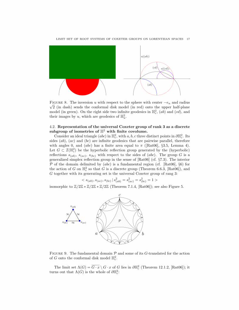
u((ab))
u((cd))(cd)
Figure 8. The inversion u with respect to the sphere with center −en and radius√2 (in dash) sends the conformal disk model (in red) onto the upper half-plane
model (in green). On the right side two infinite geodesics in H2c , (ab) and (cd), and
their images by u, which are geodesics of H2u.
4.2. Representation of the universal Coxeter group of rank 3 as a discretesubgroup of isometries of H2 with finite covolume.
Consider an ideal triangle (abc) in H2c , with a, b, c three distinct points in ∂H2
c . Itssides (ab), (ac) and (bc) are infinite geodesics that are pairwise parallel, thereforewith angles 0, and (abc) has a finite area equal to π ([Rat06], §3.5, Lemma 4).Let G ⊂ I(H2
c) be the hyperbolic reflection group generated by the (hyperbolic)reflections s(ab), s(ac), s(bc) with respect to the sides of (abc). The group G is ageneralized simplex reflection group in the sense of [Rat06] (cf. §7.3). The interiorP of the domain delimited by (abc) is a fundamental region (cf. [Rat06], §6) forthe action of G on H2
c so that G is a discrete group (Theorem 6.6.3, [Rat06]), andG together with its generating set is the universal Coxeter group of rang 3:
< s(ab), s(ac), s(bc) | s2(ab) = s2
(ac) = s2(bc) = 1 >
isomorphic to Z/2Z ∗ Z/2Z ∗ Z/2Z (Theorem 7.1.4, [Rat06]); see also Figure 5.
s(ac)
∞∞
ba
s(ab)
c
∞s(bc) P
Figure 9. The fundamental domain P and some of its G-translated for the actionof G onto the conformal disk model H2
c .
The limit set Λ(G) = G · x \G · x of G lies in ∂H2c (Theorem 12.1.2, [Rat06]); it
turns out that Λ(G) is the whole of ∂H2c :
18 C. HOHLWEG, J.-P. PREAUX, AND V. RIPOLL
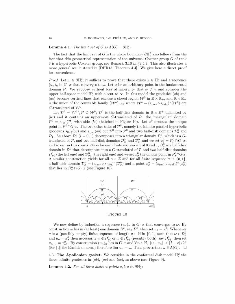
Lemma 4.1. The limit set of G is Λ(G) = ∂H2c.
The fact that the limit set of G is the whole boundary ∂H2c also follows from the
fact that this geometrical representation of the universal Coxeter group G of rank3 is a hyperbolic Coxeter group, see Remark 3.10 in §3.5.3. This also illustrates amore general result stated in [DHR13, Theorem 4.4]. We give here a direct prooffor convenience.
Proof. Let ω ∈ ∂H2c ; it suffices to prove that there exists x ∈ H2
c and a sequence(un)n in G · x that converges to ω. Let x be an arbitrary point in the fundamentaldomain P. We suppose without loss of generality that ω 6= a and consider theupper half-space model H2
u with a sent to ∞. In this model the geodesics (ab) and(ac) become vertical lines that enclose a closed region W0 in R× R+, and R× R+
is the union of the countable family (Wn)n∈Z where Wn = (s(ac) ◦ s(ab))n(W0) are
G-translated of W0.Let D0 = W0 \ P ⊂ W0; D0 is the half-disk domain in R × R+ delimited by
(bc) and it contains an uppermost G-translated of P: the ”triangular” domainP0 = s(bc)(P) with side (bc) (hatched in Figure 10). Let x0 denotes the unique
point in P0∩G·x. The two other sides of P0, namely the infinite parallel hyperbolicgeodesics s(bc)(ac) and s(bc)(ab) cut D0 into P0 and two half-disk domains D0
0 and
D01. As above D0
i (i = 0, 1) decomposes into a triangular domain P0i , which is a G-
translated of P, and two half-disk domains D0i0 and D0
i1 and we set x0i = P0
i ∩G ·x,and so on: in this construction for each finite sequence σ of 0 and 1, D0
σ is a half-diskdomain in D0 that decomposes into a G-translated of P and two half-disk domainsD0σ0 (the left one) andD0
σ1 (the right one) and we set x0σ the unique point in P0
σ∩G·x.A similar construction yields for all n ∈ Z and for all finite sequence σ in {0, 1},a half-disk domain Dnσ = (s(ac) ◦ s(ab))
n(D0σ) and a point xnσ = (s(ac) ◦ s(ab))
n(x0σ)
that lies in Dnσ ∩G · x (see Figure 10).
D0
∂H2u
D00
W0
D1
D01
W1
D000 D0
01
D10
D011D0
10
D11
D100 D1
01 D110 D1
11
b c
P0
P
Figure 10
We now define by induction a sequence (un)n in G · x that converges to ω. Byconstruction ω lies in (at least) one domain Dk, say D0, then set u0 = x0. Wheneverσ is a (possibly empty) finite sequence of length n ∈ N in {0, 1} such that ω ∈ D0
σ
and un = x0σ then necessarily ω ∈ D0
σ0 or ω ∈ D0σ1 (possibly both), say D0
σ1, then setun+1 = x0
σ1. By construction (un)n lies in G ·x and ∀n ∈ N, ‖ω−un‖ < ‖b− c‖/2n(for ‖.‖ the Euclidean norm) therefore lim un = ω. That proves that ω ∈ Λ(G). �
4.3. The Apollonian gasket. We consider in the conformal disk model H2c the
three infinite geodesics in (ab), (ac) and (bc), as above (see Figure 9).
Lemma 4.2. For all three distinct points a, b, c in ∂H2c:

LIMIT SET OF ROOT SYSTEMS OF COXETER GROUPS ON LORENTZIAN SPACES 19
(i) there exists unique horocycles ha, hb, hc with limit points a, b, c that arepairwise tangent.
(ii) (ab) intersects ha and hb perpendiculary onto the point ha ∩ hb.(iii) There exists a unique circle C passing through the intersection points ha∩hb,
ha ∩ hc and hb ∩ hc; moreover C is tangent to the three geodesics (ab), (ac)and (bc).
Proof. In the upper half space model H2u with c sent to ∞ (see Figure 11) the
horocycle hc becomes the horizontal line y = 2r, ha and hb become circles tangentto the boundary R×{0} respectively in a and b; therefore the horocycles are pairwisetangent if and only if ha, hb both have radius r and 2r = ‖a− b‖. This proves (i).The geodesics (ac) and (bc) become vertical lines x = a and x = b while (ab) is a
ha
(ac)
hb
a b
(bc)
hc
(ab)
C
H2u
Figure 11
half-circle with diameter the segment [a, b]. One obtains (ii).The three tangency points are not aligned, hence there exists a unique circle C
passing through them; it has diameter the segment with extremities ha ∩ hc andhb∩hc, radius r, and is perpendicular to the three horocycles; with (ii), C is tangentto the three geodesics. This proves (iii). �
a b
c
hc
ha
hb
a b
c
hc
ha
hb
C
Figure 12. The geodesics (ab), (ac), (ab), horocycles ha, hb, hc and the circle Cin the conformal disk model.

20 C. HOHLWEG, J.-P. PREAUX, AND V. RIPOLL
In the conformal disk model H2c the three geodesics (ab), (ac) and (bc) lie into
three unique circles, respectively C(ab), C(ac) and C(bc) of the Euclidean plane. Let
G be the subgroup of the Mobius group of R2 generated by the inversions withrespect to C(ab), C(ac), C(bc), and the circle C given by Lemma 11. The group Gof § 4.2 identifies with the subgroup generated by the inversions across C(ab), C(ac),and C(bc) and accordingly G is generated by s(ab), s(ac), s(bc) and the inversion sCwith respect to C.
Since the inversion with respect to C preserves a circle/line if and only if C in-tersects the circle/line with right angles (cf. §4.1.1), Lemma 4.2 implies that sCpreserves each of the horocycles ha, hb, hc; each one of the hyperbolic reflectionss(ab), s(ac) and s(bc) preserves the two horocycles that intersect their axis (respec-tively ha, hb, ha, hc and hb, hc) and moves the remaining one (respectively hc, hband ha) to an horocycle that remains tangent to the two others. The orbit of thethree horocycles ha, hb, hc and of ∂Hnc under the action of G yields a configura-
tion of pairwise tangent or disjoint circles in H2
c , see Figure 13. This configurationis called an Apollonian gasket A and is widely studied in the literature, see forinstance [Hir67, Max82, Gr+05, KH11, Kir13].
Figure 13. On the left (respectively right) some of the orbit of the three horocycles(respectively and of the boundary circle) under the action of G (respectively G).The complete orbit on the right figure yields the Apollonian gasket.
4.4. Discrete representation in I(H3) of the universal Coxeter group withrank 4. Consider the universal Coxeter group of rank 4 and its representation as adiscrete subgroup of OB(V ) with (V,B) = R3,1 and simple system ∆ = {α, β, γ, δ}such that for all distinct χ, ξ ∈ ∆, B(χ, ξ) = −1. In Figures 1 and 14 are represented
the polytope conv(∆) and the unit ball D31 = Q− that we identify here with H3
p.As discussed in § 3 that makes the Coxeter group Γ act on the projective ball
model by isometry (the action is given in Corollary 2.3), yielding a discrete faithfulrepresentation of Γ in I(H3
p).A direct computation shows that the reflection sα acts as the hyperbolic reflection
across the hyperbolic plane Hα = α⊥∩H3p passing through the middles of the three
edges issued from the vertex α of the tetrahedron; indeed, for example, B(α, α+β2 ) =
12 (B(α, α) + B(α, β)) = 1
2 (1 − 1) = 0 and the same computation shows that the
middles of the three edges issued from α lie in α⊥. Consider also the reflectionplanes Hβ , Hγ , Hδ (in red in Figure 14) respectively associated to sβ , sγ and sδ,

LIMIT SET OF ROOT SYSTEMS OF COXETER GROUPS ON LORENTZIAN SPACES 21
∞∞
α
∞
β
∞
∞sβ ∞
δ
γ
sδ
sα
sγ
Hδ
Figure 14. The unit ball D31 with interior identified with the projective disk model
H3p; conv(∆) is a regular tetrahedron such that the unit sphere ∂D3
1 passes through
the middles of its edges. In blue the circles on which ∂D31 intersects conv(∆). In
red the plane Hδ in H3p passing through 3 of these points.
passing through the middles of the edges adjacent respectively to the vertices β, γand δ. They are pairwise parallel and non ultra-parallel (they meet on the boundary∂H3
p), which can also be seen by cosh d(Hα,Hβ) = |B(α, β)| = 1.
The boundary sphere ∂H3p intersects the faces of the tetrahedron onto circles;
for χ = α, β, γ, δ let us denote by hχ the intersection circle on the face of thetetrahedron opposite to the vertex χ (in blue in Figure 14).
In the upper half-space model, the planes Hα, Hβ Hγ and Hδ yield a configurationof 4 half-spheres that are pairwise tangent, see Figure 15. The action of Γ restrictson ∂H3
u as the action of the subgroup G of the Mobius group on the plane (see§4.3).
∂H 3u
hγ
hβ
∂Hβ
hδ
∂Hγ
∂Hα
hα
∂Hδ
Figure 15. On the left picture: in red the four hyperbolic planes Hα, Hβ , Hγ and
Hδ (the small one in between) in the upper half-space model H3u, and in blue the
four circles hα, hβ , hγ and hδ in ∂H3u. On the right picture their intersections with
∂H3u.

22 C. HOHLWEG, J.-P. PREAUX, AND V. RIPOLL
Proposition 4.3. The limit set Λ(Γ) of Γ in H3u is the closure in ∂H3
u of theApollonian gasket A.
Proof. The two hyperplanes Hα and Hδ are parallel so denote by x0 ∈ ∂H3u their
asymptotic point. Hence the composite of the two reflections with respect to Hα andHδ is a transformation of parabolic type with limit point x0 ∈ ∂H3
u (cf. PropositionsA.5.12 and A.5.14 of [BP92]). According to Theorem 12.1.1 of [Rat06], x0 ∈ Λ(Γ).Note that x0 lies in the interior disk of R2 ≈ ∂H3
u \ {∞} delimited by the circle hδ.
The action of Γ on H3u naturally extends to a conformal action on H3
u that isthe Poincare extension of the action of the subgroup G of the Mobius group on∂H3
u ≈ R2 (cf. §4.1.3 as well as Theorem 4.4.1 of [Rat06]). As in §4.3 denote byG the subgroup of G generated by the three inversions with respect to the spheres∂Hα, ∂Hβ and ∂Hγ ; G acts on the interior of the disk delimited by ∂Hδ as the
group G of §4.2 acts on H2c . In particular Λ(Γ) contains G · x0 \G · x0 that equals
hδ (Proposition 4.1).After conjugating Γ by the reflection with respect to Hα (respectively Hβ , Hγ)
the same argument applies to show that Λ(Γ) contains also hα (respectively hβ , hγ).Hence the Apollonian gasket A, as seen in §4.3, which is the orbit of hα∪hb∪hγ∪hδunder the action of G, is a Γ-invariant subset of Λ(Γ); since Λ(Γ) is closed in∂H3
u (Theorem 12.1.2, Corollary 1 of [Rat06]) the closure A of A in ∂H3u is a
closed Γ-invariant subset of ∂H3u contained in Λ(Γ). Since Λ(Γ) is infinite, Γ is non
elementary (cf. Theorem 12.2.1 of [Rat06]) and therefore any closed Γ-invariantsubset of ∂H3
u contains Λ(Γ) (Theorem 12.1.3 of [Rat06]). Hence Λ(Γ) equals A. �
Figure 16. The Apollonian gasket in ∂H3u whose closure is the limit set of Γ. In
both the conformal and projective ball models one obtains as limit set the Apollo-nian packing of the sphere as in Figure 1.
The closure A of A is the complement in the closed external disk (delimited byhδ) of the union of the interiors of disks delimited by the circles of the gasket.

LIMIT SET OF ROOT SYSTEMS OF COXETER GROUPS ON LORENTZIAN SPACES 23
References
[AB08] P. Abramenko and K. S. Brown. Buildings, Theory and Applications, volume 248 ofGTM. Springer, New York, 2008.
[AVS93] D. V. Alekseevskij, E. B. Vinberg, and A. S. Solodovnikov. Geometry of spaces of
constant curvature. In Geometry, II, volume 29 of Encyclopaedia Math. Sci., pages1–138. Springer, Berlin, 1993.
[BP92] R. Benedetti and C. Petronio. Lectures on hyperbolic geometry. Universitext,
Springer, 1992.[Bou68] N. Bourbaki. Groupes et algebres de Lie, Chapitres IV–VI. Actualites Scientifiques
et Industrielles, No. 1337. Hermann, Paris, 1968.
[Cox34] H. S. M. Coxeter. Discrete groups generated by reflections. Ann. of Math., 35:588–621, 1934.
[Dav08] M. W. Davis. The Geometry and Topology of Coxeter Groups, volume 32. London
Mathematical Society Monographs, 2008.[Dol08] Igor V. Dolgachev. Reflection groups in algebraic geometry. Bull. Amer. Math. Soc.
(N.S.), 45(1):1–60, 2008.[DHR13] M. Dyer, C. Hohlweg, and V. Ripoll. Imaginary cones and limit roots of infinite
Coxeter groups. 2013. arxiv.org/abs/1303.6710.
[Dye12] M. Dyer. Imaginary cone and reflection subgroups of Coxeter groups. 2012. arXiv:1210.5206.
[Edg09] T. Edgar. Dominance and regularity in coxeter groups. PhD Thesis, University of
Notre Dame, 2009. http://etd.nd.edu/ETD-db/.[Fu11] X. Fu. Coxeter groups, imaginary cones and dominance. 2011.
http://arxiv.org/abs/1108.5232.
[Gr+05] R.L. Graham, L.J. Lagarias, C.L. Mallows, A.R. Wilks, C.H. Yan. Apollonian circlepackings: geometry and group theory. I. The Apollonian group. Discrete Comput.
Geom. 34(4) (2005): 547-585.
[Hee93] J.-T. Hee. Sur la torsion de Steinberg-Ree des groupes de Chevalley et des groupesde Kac-Moody. PhD Thesis, Universite Paris-Sud, Orsay of Notre Dame, 1993.
[HMN12] Akihiro Higashitani, Ryosuke Mineyama, and Norihiro Nakashima. A metric analysis
of infinite Coxeter groups : the case of type (n − 1, 1) Coxeter matrices. PreprintarXiv:1212.6617 http://arxiv.org/abs/1212.6617, last revised April 2013.
[Hir67] K.E. Hirst. The Apollonian packing of circles. J. London Math. Soc. 42 (1967): 281-291.
[HLR11] C. Hohlweg, J.-P. Labbe, and V. Ripoll. Asymptotical behaviour of roots of infinite
Coxeter groups. 2011. http://arxiv.org/abs/1112.5415.[Hum90] J. E. Humphreys. Reflection groups and Coxeter groups, volume 29. Cambridge Uni-
versity Press, Cambridge, 1990.
[Kac90] V. G. Kac. Infinite-dimensional Lie algebras. Cambridge University Press, Cam-bridge, third edition, 1990. http://dx.doi.org/10.1017/CBO9780511626234.
[Kir13] A.A. Kirillov. A tale of two fractals. Birkhauser Boston Inc. 2013.
[KH11] A. Kontorovich and Hee Oh. Apollonian circle packings and closed horospheres onhyperbolic 3-manifolds. J. Amer. Soc. 24 (2011): 603-648.
[Kra09] D. Krammer. The conjugacy problem for Coxeter groups. Groups Geom. Dyn.,3(1):71–171, 2009. http://dx.doi.org/10.4171/GGD/52.
[MT98] Katsuhiko Matsuzaki and Masahiko Taniguchi. Hyperbolic manifolds and Kleiniangroups. Oxford Mathematical Monographs. The Clarendon Press Oxford UniversityPress, New York, 1998. Oxford Science Publications.
[Max82] G. Maxwell. Sphere packing and hyperbolic reflection groups. J. of Algebra 79 (1982):
78-97.[Nic89] Peter J. Nicholls. The ergodic theory of discrete groups, volume 143 of London Math-
ematical Society Lecture Note Series. Cambridge University Press, Cambridge, 1989.[Rat06] John G. Ratcliffe. Foundations of hyperbolic manifolds, volume 149 of Graduate
Texts in Mathematics. Springer, New York, second edition, 2006.
[S+11] William A. Stein et al. Sage Mathematics Software (Version 4.7.2). The Sage De-
velopment Team, 2011. http://www.sagemath.org.

24 C. HOHLWEG, J.-P. PREAUX, AND V. RIPOLL
[Vin71] E. B. Vinberg. Discrete linear groups that are generated by reflections. Izv. Akad.
Nauk SSSR Ser. Mat., 35:1072–1112, 1971. Translation by P. Flor, IOP Science.
[VS93] E. B. Vinberg and O. V. Shvartsman. Discrete groups of motions of spaces of constant
curvature. In Geometry, II, volume 29 of Encyclopaedia Math. Sci., pages 139–248.Springer, Berlin, 1993.
(Christophe Hohlweg) Universite du Quebec a Montreal, LaCIM et Departement de
Mathematiques, CP 8888 Succ. Centre-Ville, Montreal, Quebec, H3C 3P8, CanadaE-mail address: [email protected]
URL: http://hohlweg.math.uqam.ca
(Jean-Philippe Preaux) Laboratoire d’Analyse, Topologie et Probabilites, UMR CNRS
7353, 39 rue Joliot-Curie, 13453 Marseille cedex, France
E-mail address: [email protected]
URL: http://www.cmi.univ-mrs.fr/~preaux
(Vivien Ripoll) Universite du Quebec a Montreal, LaCIM et Departement de Mathe-matiques, CP 8888 Succ. Centre-Ville, Montreal, Quebec, H3C 3P8, Canada
E-mail address: [email protected]