on the inverse problem of constructing - citeseer
TRANSCRIPT
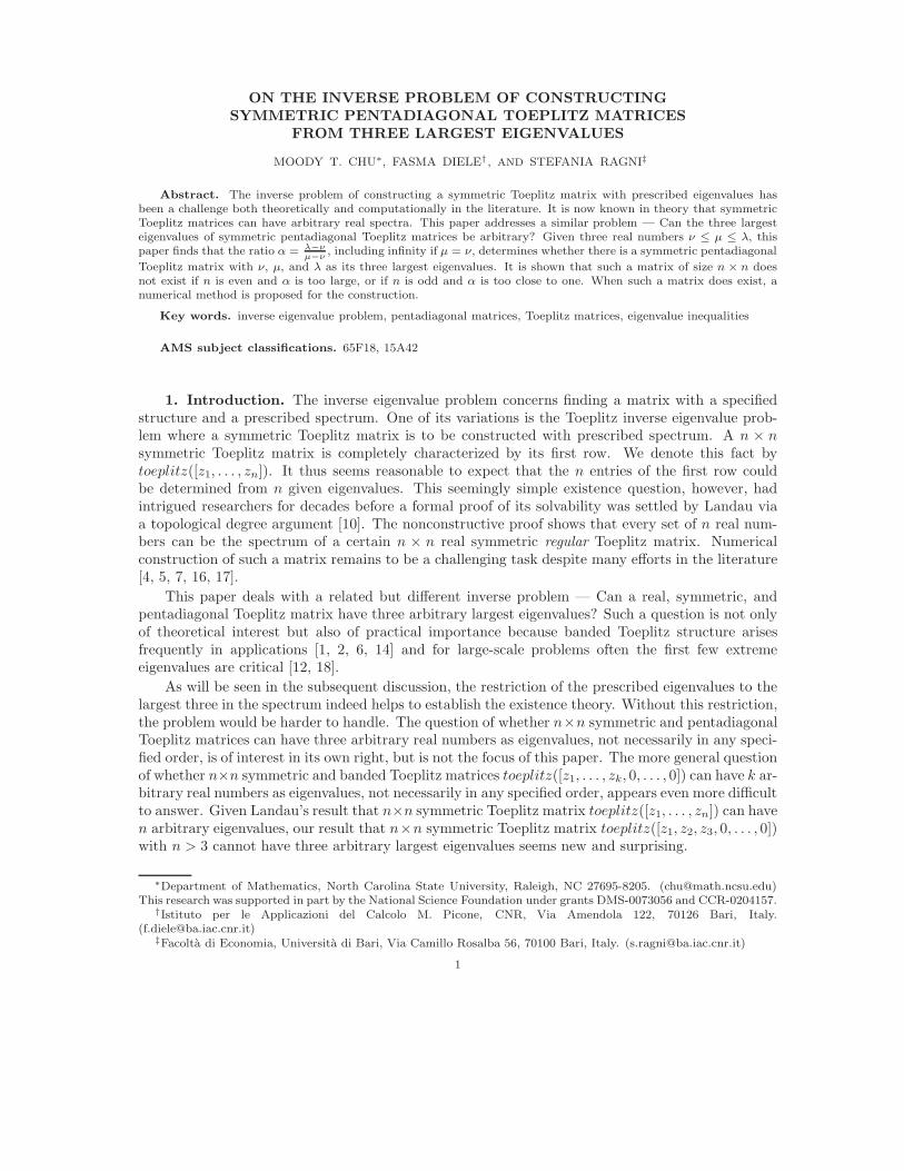
ON THE INVERSE PROBLEM OF CONSTRUCTING
SYMMETRIC PENTADIAGONAL TOEPLITZ MATRICES
FROM THREE LARGEST EIGENVALUES
MOODY T. CHU∗, FASMA DIELE† , AND STEFANIA RAGNI‡
Abstract. The inverse problem of constructing a symmetric Toeplitz matrix with prescribed eigenvalues hasbeen a challenge both theoretically and computationally in the literature. It is now known in theory that symmetricToeplitz matrices can have arbitrary real spectra. This paper addresses a similar problem — Can the three largesteigenvalues of symmetric pentadiagonal Toeplitz matrices be arbitrary? Given three real numbers ν ≤ µ ≤ λ, thispaper finds that the ratio α = λ−ν
µ−ν, including infinity if µ = ν, determines whether there is a symmetric pentadiagonal
Toeplitz matrix with ν, µ, and λ as its three largest eigenvalues. It is shown that such a matrix of size n × n doesnot exist if n is even and α is too large, or if n is odd and α is too close to one. When such a matrix does exist, anumerical method is proposed for the construction.
Key words. inverse eigenvalue problem, pentadiagonal matrices, Toeplitz matrices, eigenvalue inequalities
AMS subject classifications. 65F18, 15A42
1. Introduction. The inverse eigenvalue problem concerns finding a matrix with a specifiedstructure and a prescribed spectrum. One of its variations is the Toeplitz inverse eigenvalue prob-lem where a symmetric Toeplitz matrix is to be constructed with prescribed spectrum. A n × nsymmetric Toeplitz matrix is completely characterized by its first row. We denote this fact bytoeplitz([z1, . . . , zn]). It thus seems reasonable to expect that the n entries of the first row couldbe determined from n given eigenvalues. This seemingly simple existence question, however, hadintrigued researchers for decades before a formal proof of its solvability was settled by Landau viaa topological degree argument [10]. The nonconstructive proof shows that every set of n real num-bers can be the spectrum of a certain n × n real symmetric regular Toeplitz matrix. Numericalconstruction of such a matrix remains to be a challenging task despite many efforts in the literature[4, 5, 7, 16, 17].
This paper deals with a related but different inverse problem — Can a real, symmetric, andpentadiagonal Toeplitz matrix have three arbitrary largest eigenvalues? Such a question is not onlyof theoretical interest but also of practical importance because banded Toeplitz structure arisesfrequently in applications [1, 2, 6, 14] and for large-scale problems often the first few extremeeigenvalues are critical [12, 18].
As will be seen in the subsequent discussion, the restriction of the prescribed eigenvalues to thelargest three in the spectrum indeed helps to establish the existence theory. Without this restriction,the problem would be harder to handle. The question of whether n×n symmetric and pentadiagonalToeplitz matrices can have three arbitrary real numbers as eigenvalues, not necessarily in any speci-fied order, is of interest in its own right, but is not the focus of this paper. The more general questionof whether n×n symmetric and banded Toeplitz matrices toeplitz([z1, . . . , zk, 0, . . . , 0]) can have k ar-bitrary real numbers as eigenvalues, not necessarily in any specified order, appears even more difficultto answer. Given Landau’s result that n×n symmetric Toeplitz matrix toeplitz([z1, . . . , zn]) can haven arbitrary eigenvalues, our result that n×n symmetric Toeplitz matrix toeplitz([z1, z2, z3, 0, . . . , 0])with n > 3 cannot have three arbitrary largest eigenvalues seems new and surprising.
∗Department of Mathematics, North Carolina State University, Raleigh, NC 27695-8205. ([email protected])This research was supported in part by the National Science Foundation under grants DMS-0073056 and CCR-0204157.
†Istituto per le Applicazioni del Calcolo M. Picone, CNR, Via Amendola 122, 70126 Bari, Italy.([email protected])
‡Facolta di Economia, Universita di Bari, Via Camillo Rosalba 56, 70100 Bari, Italy. ([email protected])
1

It is well known that the spectrum of the n × n symmetric and tridiagonal Toeplitz matrixtoeplitz([a, b, 0, . . .0]) consists of values
µn+1−k = a + 2b coskπ
n + 1, k = 1, . . . n. (1.1)
Given any two arbitrary real values µn−1 < µn, it is clear that, because the cosine function is strictlydecreasing over the interval (0, π), values a and b can be found so that toeplitz([a, b, 0, . . .0]) hasµn−1, µn as its first two largest eigenvalues. Once a and b are fixed, the third largest eigenvalueµn−2 is necessarily determined.
Throughout this note, let An := An(a, b, c) denote the n × n symmetric and pentadiagonalToeplitz matrix
An(a, b, c) := toeplitz([a, b, c, 0, ..., 0]). (1.2)
Without loss of generality, we shall rule out the case c = 0. For reasons that will become clear later,we shall also assume temporarily that c > 0. Let Bn = Bn(γ) denote the associate matrix,
Bn(γ) := toeplitz([0, γ, 1, 0, ..., 0]), (1.3)
where γ := b/c. Assume that all eigenvalues are arranged in ascending order, that is, λ1(An) ≤ . . . ≤λn(An) and so on. It is obvious that eigenvalues λi(An) of An are related to eigenvalues λi(Bn) viathe relationship
a + cλi(Bn) = λi(An). (1.4)
It follows that, from given any two sets of eigenvalues λi(An), λj(An) and λi(Bn), λj(Bn), wecan solve
a =λj(Bn)λi(An) − λi(Bn)λj(An)
λj(Bn) − λi(Bn), (1.5)
c =λj(An) − λi(An)
λj(Bn) − λi(Bn), (1.6)
provided λj(Bn) 6= λi(Bn). Plugging in a and c for any other λk(Bn), we see that
λk(Bn) = αλj(Bn) + (1 − α)λi(Bn), (1.7)
with
α =λk(An) − λi(An)
λj(An) − λi(An). (1.8)
The inverse eigenvalue problem for the symmetric and pentadiagonal Toeplitz matrix An thereforecan be reformulated as follows:
Given three (largest) eigenvalues λi(An) < λj(An) < λk(An) of An, find the scalar γ suchthat Bn(γ) has three eigenvalues λi(Bn) < λj(Bn) < λk(Bn) = αλj(Bn) + (1 − α)λi(Bn)with α defined by (1.8).
We shall refer to this problem as the inverse problem for the matrix Bn(γ).The difference quotient relationship,
λk(An) − λi(An)
λj(An) − λi(An)=
λk(Bn) − λi(Bn)
λj(Bn) − λi(Bn)= α, (1.9)
between three ordered eigenvalues of An and Bn follows from (1.7). Observe the clear advantagethat there is only one free parameter γ involved in the matrix Bn(γ). Our understanding about thespectrum of the simpler Bn(γ) will shed considerable insights into the inverse eigenvalue problemfor the An by using the relationship (1.9) as we explain below.
2

2. Preliminaries. While the spectra of B2n(γ) and B2n−1(γ) share many similar properties,the even or odd dimensionality does have different effect on the solvability of the inverse problem.To prepare for the investigation, we first introduce some fundamental facts about the spectrum ofBn(γ) in general. A series of results that eventually build up the answer to the question of solvabilityfor the inverse problem of pentadiagonal Toeplitz matrix with three prescribed largest eigenvalueswill be derived in the sequel. We believe that some of the results presented in this section are newand are of interest in their own right.
By writing Bn(γ)γ
= toeplitz([0, 1, 1/γ, 0, . . . , 0]) and using (1.1), the following asymptotic be-havior is clear.
Lemma 2.1. Let the eigenvalues λ1(Bn(γ)) ≤ . . . ≤ λn(Bn(γ)) be arranged in increasing order.Then
limγ→±∞
λn+1−k(Bn(γ))
γ= ±2 cos
kπ
n + 1, k = 1, . . . , n. (2.1)
There is a recursive relation for the determinant of a pentadiagonal matrix [15]. In particular,denote the characteristic polynomial of Ak by
ρk = ρk(λ; a, b, c) := det(Ak − λI), (2.2)
then the following fact can be derived.Theorem 2.2. Define ρ−1 := 0, ρ0 := 1, ρ1 := a − λ, ρ2 := (a − λ)2 − b2, and ρ3 :=
(a − λ)3−2 (a − λ) b2 +2cb2− (a − λ) c2. Then for k = 4, 5, . . ., the polynomial ρk satisfies a 6-term
recursion relationship
ρk := (a − λ − c) ρk−1 −(
b2 − (a − λ) c)
ρk−2 −(
(a − λ) c2 − b2c)
ρk−3
+c2(
c2 − (a − λ) c)
ρk−4 + c5ρk−5. (2.3)
Let the characteristic polynomial of Bk(γ) be noted by
k = k(λ; γ) = det(Bk − λI).
With −1 := 0, 0 := 1, 1 := −λ, 2 := λ2 − γ2, and 3 := −λ3 + 2λγ2 + 2γ2 + λ, we see from theabove theorem that for k ≥ 4, k is given recursively by
k = − (1 + λ) k−1 −(
γ2 + λ)
k−2 +(
γ2 + λ)
k−3 + (1 + λ) k−4 + k−5,
which clearly is an even function in γ.Corollary 2.3. Both Bn(γ) and Bn(−γ) have the same characteristic polynomial and, hence,
the same set of eigenvalues.Additional symmetry on the eigenvalues of Bn(γ) can be obtained from exploiting its centrosym-
metric structure. We shall demonstrate the case for B2n only. A similar argument can be carriedout for B2n−1(γ). Let Ξn = [ξij ] denote the n × n standard involution permutation matrix, that is,the perdiagonal matrix whose entries are defined by
ξij =
1 if i = n + 1 − j,0 otherwise.
Any 2n× 2n centrosymmetric matrix M2n is of the form [3]
M2n =
[
Xn Y ⊤n
Yn ΞnXnΞn
]
,
3

where Xn, Yn ∈ Rn×n and Xn is symmetric. Define the orthogonal matrix
K2n :=1√2
[
In −Ξn
In Ξn
]
,
where In is the n × n identity matrix. It is not difficult to see that
K2nM2nKT2n =
[
Xn − ΞnYn 00 Xn + ΞnYn
]
.
The spectra of Xn ∓ ΞnYn are known as eigenvalues of M2n with odd and even parity, respectively.Upon applying the same orthogonal similarity transformation to M2n = B2n(γ) of size 2n× 2n, weobserve the structure where the corresponding n× n matrices Xn ∓ΞnYn of B2n(γ) are of the form
0 γ 1 0 . . . 0γ 0 γ 1 01 γ 0 γ
. . .
. . .
γ 1 0γ 0 γ 1
0 1 γ 0 γ ∓ 10 0 0 0 1 γ ∓ 1 ∓γ
, (2.4)
respectively. Let
f(λ; γ) := det(Xn − ΞnYn − λI),
g(λ; γ) := det(Xn + ΞnYn − λI),
denote the characteristic polynomials of Xn∓ΞnYn, respectively. Then it is easy to see that f(λ; γ) =g(λ;−γ). A similar argument can be applied to B2n−1(γ). We therefore have proved another spectralproperty of Bn.
Lemma 2.4. The very same eigenvalue of B2n(γ) and B2n(−γ) has opposite parity whereas thevery same eigenvalue of B2n−1(γ) and B2n−1(−γ) maintains the same parity.
By the symmetry described in Corollary 2.3 and Lemma 2.4, it suffices to consider for our inverseproblem the case γ ≥ 0 only. The inverse problem is solvable for some γ if and only if it is solvablefor some γ ≥ 0 and, in this case, it is also solvable for −γ. Furthermore, the eigenstructure of thematrix Bn(0) for the special case of γ = 0 is easy. Indeed, let the Gauss brackets ⌈·⌉ and ⌊·⌋ denotethe smallest integer greater than and the largest integer not greater than the number they embrace,respectively. Then Bn(0) can be effectively reduced by permutations to two tridiagonal Toeplitzmatrices toeplitz([0, 1, 0, . . . , 0]) of size ⌈n/2⌉ and ⌊n/2⌋, respectively, whose eigenvalues are knownaccording to (1.1).
Lemma 2.5. The eigenvalues of B2n−1(0) are all simple and, if listed in ascending order,alternate the parities with the largest eigenvalue even. Each eigenvalue of B2n(0) is always a doubleeigenvalue.
Henceforth, we shall limit our attention to the case γ > 0 only. Immediately, we find that thelargest eigenvalue has the following characteristics.
Theorem 2.6. If γ > 0, then the largest eigenvalue of Bn(γ) is positive, simple, and has aneven parity.
Proof. Since γ > 0, the matrix Bn(γ) is irreducible and nonnegative. The well-known Perron-Frobenius Theorem [8, Theorem 8.4.4] asserts that the spectral radius of Bn(γ) is precisely the
4

largest eigenvalue λn(Bn(γ)) of Bn(γ) and that λn(Bn(γ)) is simple. The corresponding eigenvectoris necessarily of one sign and, hence, must be an even vector.
For later reference, we recall a special case of the well-known Courant-Fischer Theorem. Thecondition where equalities hold is of particular importance to us.
Theorem 2.7. Let P ∈ Rn×m be such that P⊤P = Im. Let S ∈ R
n×n be symmetric and defineT := P⊤SP . Let the spectra of S and T be denoted as θ1 ≤ . . . ≤ θn and τ1 ≤ . . . ≤ τm, respectively.Then the interlacing property
θj ≤ τj ≤ θn−m+j
holds for 1 ≤ j ≤ m. If θj = τj for some j, then there exists a vector v ∈ Rm such that
Tv = τjv,
SPv = θjPv.
Proof. The fact that the spectra of S and T interlace with each other can be found in manyreferences. See, for example, [8, Theorem 4.2.1]. For completion, however, we briefly outline theproof with emphasis on the case when one of the equalities hold.
Let u1, . . . ,un be an orthonormal basis of eigenvectors of S and let v1, . . . ,vm be such abasis for T . Denote the invariant subspaces spanned by u1, . . . ,ui and by v1, . . . ,vj by Ui andVj , respectively. It is clear that, given any u ∈ U⊥
j−1 and v ∈ Vj ,
v⊤Tv ≤ τjv⊤v, (2.5)
u⊤Su ≥ θju⊤u. (2.6)
Suppose that the equality in (2.5) holds. Write v =∑j
i=1 ξivi. Then
τj
j∑
i=1
ξ2i = v⊤Tv =
j∑
i=1
ξ2i τi ≤ τj−1
j−1∑
i=1
ξ2i + τjξ
2j .
It follows that either∑j−1
i=1 ξ2i = 0 or τj = τj−1. In the former, v is parallel to vj and, hence, is an
eigenvector. In the latter, we can replace the inequality by
τj
j∑
i=1
ξ2i = v⊤Tv =
j∑
i=1
ξ2i τi ≤ τj−2
j−2∑
i=1
ξ2i + τjξ
2j−1 + τjξ
2j .
We thus conclude that either v belongs to the eigenspace spanned by vj−1,vj or τj = τj−1 = τj−2.The process can be continued and must terminate in finitely many steps. In all cases, v is aneigenvector corresponding to the eigenvalue τj . Similarly, if the equality in (2.6) holds, then u mustbe an eigenvector corresponding to the eigenvalue θj .
It is clear that the subspace Vj
⋂
(P⊤Uj−1)⊥ ⊂ R
m is of dimension at least one. Let v be anonzero vector in Vj
⋂
(P⊤Uj−1)⊥. Then it must be the case that Pv ∈ U⊥
j−1. It follows that
θj ≤ v⊤P⊤SPv
v⊤P⊤Pv=
v⊤Tv
v⊤v≤ τj .
In the event that θj = τj for some j, we see that the vector v ∈ Vj
⋂
(P⊤Uj−1)⊥ is an eigenvector
of T with eigenvalue τj and Pv is an eigenvector of S with eigenvalue θj .
5

By applying a similar argument, the other inequality can be established. In particular, thereexists a nonzero vector v ∈ V ⊥
j−1
⋂
(P⊤U⊥n−m+j)
⊥ such that
τj ≤ v⊤Tv
v⊤v=
v⊤P⊤SPv
v⊤P⊤Pv≤ θn−m+j .
If θn−m+j = τj for some j, we see that the vector v ∈ V ⊥j−1
⋂
(P⊤U⊥n−m+j)
⊥ is an eigenvector of Twith eigenvalue τj and Pv ∈ Un−m+j is an eigenvector of S with eigenvalue θn−m+j .
It is not difficult to calculate that the second largest eigenvalue of B4(γ) is given by
λ3(B4(γ)) =
√
5γ2 − 8γ + 4 − γ
2.
By the interlacing property, we know that λk−1(Bk(γ)) ≥ λ3(B4(γ)) for all k ≥ 4. We thus confirmthe nonnegativity of the second largest eigenvalue.
Lemma 2.8. For k ≥ 4, the second largest eigenvalue λk−1(Bk(γ)) is always nonnegative.We next address the algebraic multiplicity of eigenvalues of Bn(γ).Theorem 2.9. If γ > 0, then any eigenvalue of the matrix Bn(γ) can have multiplicity at most
two.
Proof. We shall prove the result by induction. Eigenvalues of B3(γ) are −1 and1±
√1+8γ2
2 . Itis clear that any eigenvalue can have multiplicity at most two.
Assume that the assertion is true for Bℓ(γ). Let u1, . . . ,uℓ+1 be an orthonormal basis ofeigenvectors corresponding to eigenvalues θ1, . . . , θℓ+1 of Bℓ+1. Likewise, let v1, . . . ,vℓ be sucha basis for Bℓ with eigenvalues τ1, . . . , τℓ. Denote the invariant subspaces spanned by u1, . . . ,uiand by v1, . . . ,vj by Ui and Vj , respectively. By Theorem 2.7, the interlacing relationship
θj−1 ≤ τj−1 ≤ θj ≤ τj ≤ θj+1
holds for all 1 ≤ j ≤ ℓ.Suppose that for some j, θj−1 = θj = θj+1. Then using arguments given in the proof of
Theorem 2.7, we are certain that there exist eigenvectors x,y ∈ Rℓ of Bℓ(γ) from the subspaces
x ∈ Vj−1
⋂
(P⊤Uj−2)⊥,
y ∈ V ⊥
j−1
⋂
(P⊤U⊥
j+1)⊥,
respectively, such that [x⊤, 0]⊤, [y⊤, 0]⊤ ∈ Rℓ+1 are eigenvectors of Bℓ+1(γ). It follows that x ⊥ y
and, hence, are linearly independent. By assumption, any other eigenvector of Bℓ(γ) with eigenvalueτj must be a linear combination of x and y, and vice versa. In particular, Ξℓx and Ξℓy are alsoeigenvectors of Bℓ(γ). Without loss of generality, we may now assume that x is an even vector andy is an odd vector. It then follows that both x and y have nonzero first entries.
Recall that Ξℓ+1Bℓ+1(γ)Ξℓ+1 = Bℓ+1(γ). It follows that all four vectors
[
x
0
]
,
[
0x
]
,
[
y
0
]
,
[
0−y
]
,
are eigenvectors of Bℓ+1. With the fact that x ⊥ y, it is not difficult to check that these four vectorsare necessarily independent, implying that θj is of multiplicity at least four. By the interlacingproperty, it would imply that τj is of multiplicity at least three, contradicting with the assumptionin the induction.
Note that the family of matrices Bn(γ) depends analytically on the parameter γ, it is a classicalresult that Bn(γ) enjoys an analytic Schur decomposition [9, 13]. In particular, at any simple
6

eigenvalue λ0 of Bn(γ0) there exists a neighborhood of γ0 in which both the eigenvalue λ(γ) andthe corresponding unit eigenvector v(γ) are analytic in γ. It is easy to see that the eigenvalue curveλ(γ) satisfies the initial value problem
dλ(γ)
dγ= v(γ)⊤Cv(γ), λ(γ0) = λ0 (2.7)
where C := toeplitz([0, 1, 0, . . . , 0]). This differential equation relationship remains valid even if λ0
is a multiple eigenvalue. Indeed, if ǫm is a sequence of nonzero real numbers tending to 0 for whichlimm→∞ v(γ0 + ǫm) = u(γ0) exists, then the limit
limm→∞
λ(γ0 + ǫm) − λ(γ0)
ǫm
= µ(γ0)
also exists [13, Page 45]. In this case, it can be proved that Bn(γ0)u(γ0) = λ0u(γ0) and µ(γ0) =u(γ0)
⊤Cu(γ0). We claim that these eigenvalue curves intersect transversally at multiple eigenvaluesin the following sense.
Theorem 2.10. If x and y are two orthonormal eigenvectors of Bn(γ0) corresponding to thesame eigenvalue λ0, then x⊤Cx 6= y⊤Cy.
Proof. By Theorem 2.9, x and y form the basis of the eigenspace Ω corresponding to λ0 forBn(γ0). That is, Ω is of dimension two.
Assume that x⊤Cx = y⊤Cy = α Then w⊤Cw = α for every unit vector w in Ω. Note thatBn(γ) = γC + E where E := toeplitz([0, 0, 1, 0, . . . , 0]). From the fact that λ0 = x⊤Bn(γ0)x =y⊤Bn(γ0)y, we must have x⊤Ex = y⊤Ey = β. This would imply that at every γ ∈ R it is alwaysthe case that w⊤Bn(γ)w ≡ γα + β for every unit vector w ∈ Ω, which is not possible .
For any fixed γ0 ∈ R, denote
a := v(γ0)⊤Cv(γ0),
b := v(γ0)⊤Ev(γ0),
where v(γ0) is the unit eigenvector of Bn(γ0) corresponding to the largest eigenvalue λn(Bn(γ0)).Since
u⊤Bn(γ)u = γu⊤Cu + u⊤Eu ≤ λn(Bn(γ))
for all unit vectors u ∈ Rn, it follows that
aγ + b ≤ λn(Bn(γ)) (2.8)
for all γ ∈ R. This inequality (2.8) together with its equality at γ0 shows that largest eigenvaluecurve λn(Bn(γ)) of Bn(γ) is being supported below by the straight line y = aγ + b at γ0. Indeed,such a support exists at every γ0. This shows the convexity of λn(Bn(γ)). A similar argument canbe given for the smallest eigenvalue curve which we summarize as follows [13, Page 42].
Lemma 2.11. The largest eigenvalue λn(Bn(γ)) is a convex function of γ while the smallesteigenvalue λ1(Bn(γ)) is a concave function of γ.
3. Solvability. The recursive formula (2.3) can be employed as a numerical means to constructa symmetric and pentadiagonal Toeplitz matrix with three prescribed eigenvalues. We will discusslater how the recursion can be compacted into matrix form which facilitates the computation. Beforesuch an endeavor, however, a more fundamental question is whether the inverse problem is solvable.Toward that end, for fixed indices i, j and k, define the subset Rijk of real numbers by
Rijk :=
λk(Bn) − λi(Bn)
λj(Bn) − λi(Bn)|γ ∈ R
. (3.1)
7

The range of Rijk plays a critical role in the solvability according to the following observation.
Theorem 3.1. The inverse eigenvalue problem for An is solvable for any eigenvalues λi(An) <λj(An) < λk(An) if and only if Rijk = [1,∞). If Rijk is bounded in the interval [ζ, η], then theinverse eigenvalue problem is not solvable if
λk(An) − λi(An)
λj(An) − λi(An)> η, or
λk(An) − λi(An)
λj(An) − λi(An)< ζ.
Proof. The given ordered triplet λi(An) < λj(An) < λk(An) determines a value for α accordingto (1.8). In the meantime, by (1.9), α is a function of γ. Any value of α in the range of Rijk
corresponds to at least one value of γ which, in turn, determines the ordered triplet λi(Bn) <λj(Bn) < λk(bn). Finally, values of a and c are determined from equations (1.4) and b = cγ.
A simple numerical experiment with the case n = 4 illustrates the significance of Theorem 3.1.In Figure 3.1, the eigenvalues of B4(γ) = toeplitz([0, γ, 1, 0]) are plotted against γ ∈ [−20, 20].Many of the properties described earlier are manifested in this figure. The ratio α defined in (1.9)
−20 −15 −10 −5 0 5 10 15 20−40
−30
−20
−10
0
10
20
30
40
γ
λ(B
)
Eigenvalues of toeplitz([0,γ,1,0])
Fig. 3.1. Distribution of eigenvalues of toeplitz([0, γ, 1, 0]).
by the three largest eigenvalues of B4(γ) is plotted in the left drawing in Figure 3.2. It appears thatthe set R234 should be bounded. A test of 500 matrices A4 = toeplitz([a, b, c, 0]) with entries a, band c randomly generated from the standard normal distribution, depicted in the right drawing ofFigure 3.2, seems to reaffirm this observation. Although Landau’s result asserts that 1, 2, 6 is thespectrum of a certain 3 × 3 symmetric Toeplitz matrix toeplitz([a, b, c]), this experiment seems tosuggest that no symmetric Toeplitz matrix toeplitz([a, b, c, 0]) can have 1, 2, 6 as its three largesteigenvalues because the ratio α = 5 is too large. We shall investigate the general case in more details.We separate discussion into two cases.
3.1. Even Dimension. Trivially, the difference quotient α of the three largest eigenvalues ofany (symmetric) matrix is at least 1. We know by Lemma 2.5 that this minimal ratio for B2n(γ)is attainable at γ = 0. Numerical experiments suggest that the ratio α from the three largesteigenvalues of B2n(γ) is always bounded above. If this is true, then it would imply that the three
8

−20 −15 −10 −5 0 5 10 15 2010
0
γ
α =
(λ
n(B
)−λ
n−
2(B
))/(
λn
−1(B
)−λ
n−
2(B
))
Range of α
0 50 100 150 200 250 300 350 400 450 500
100.1
100.2
100.3
100.4
100.5
number of random test
α =
(λ
n(B
)−λ
n−
2(B
))/(
λn
−1(B
)−λ
n−
2(B
))
Distribution of Ratio α from 500 Random toeplitz([a,b,c,0])
Fig. 3.2. Attainable ratio α from γ and from 500 random tests.
largest eigenvalues of pentadiagonal Toeplitz matrices cannot be arbitrarily assigned. In this sectionour goal is to prove the following theorem.
Theorem 3.2. Assume that n is even. The inverse problem of constructing a n×n symmetricpentadiagonal Toeplitz matrix with three given real numbers as its largest eigenvalues is not solvableif the ratio α determined by the three given numbers is too large.
For convenience, denote the even dimensionality by 2n. Let P ∈ R2n×(2n−1) be the matrix
by deleting the last column of the identity matrix I2n. Then B2n−1 = P⊤B2nP . The interlacingbetween the largest few eigenvalues of B2n−1(γ) and B2n(γ) is stated as
λ2n−2(B2n) ≤ λ2n−2(B2n−1) ≤ λ2n−1(B2n) ≤ λ2n−1(B2n−1) ≤ λ2n(B2n). (3.2)
Furthermore, observe that Xn−1 ∓Ξn−1Yn−1 are principal submatrices of Xn ∓ ΞnYn, respectively.By the interlacing eigenvalues theorem for bordered matrices [8], the odd and even eigenvalues ofB2n(γ) interlace with the odd and even eigenvalues of B2(n−1)(γ), respectively. Such a relationshipbetween B4(γ) and B6(γ) is illustrated in Figure 3.3.
We have already proved in Theorem 2.6 that the largest eigenvalue of Bn(γ) is simple, positive,and even for every n. We also know from Lemma 2.8 that the second largest eigenvalue of Bn(γ) isalways nonnegative, if n ≥ 4. We now address the parity of λ2n−1(B2n).
Lemma 3.3. If γ > 0, then the second largest eigenvalue of B2n(γ) is odd unless it has multi-plicity greater than one.
Proof. We know that the even and odd eigenvalues of B2n correspond to eigenvalues of Xn+ΞnYn
and Xn − ΞnYn, respectively. By Theorem 2.6, the largest eigenvalue of B2n(γ) is λn(Xn + ΞnYn).So we only need to compare the second largest eigenvalue λn−1(Xn + ΞnYn) of Xn + ΞnYn with the
9

−4 −3 −2 −1 0 1 2 3 4−6
−4
−2
0
2
4
6
8
10
Interlacing between X2−Ξ
2Y
2 and X
3−Ξ
3Y
3
γ
λ
Fig. 3.3. The interlacing between eigenvalues of X2 − Ξ2Y2 (boldfaced solid line) and X3 − Ξ3Y3 (boldfaceddashed line). The interlacing of even eigenvalues of B4(γ) and B6(γ) are mirror images drawn in thinner lines.
largest eigenvalue λn(Xn − ΞnYn) of Xn − ΞnYn. From (2.4), we see that
C := (Xn + ΞnYn) − (Xn − ΞnYn) =
0 0 00...
. . .
0 0 0 20 2 2γ
,
which has eigenvalues γ −√
γ2 + 4, 0, . . . , 0, γ +√
γ2 + 4. By the Weyl theorem [8, Theorem 4.3.1],we know that
λn−1(Xn + ΞnYn) ≤ λn(Xn − ΞnYn) + λn−1(C).
The second largest eigenvalue of B2n(γ) therefore is λn(Xn − ΞnYn) because λn−1(C) = 0.
We are now ready to prove the key result.
Theorem 3.4. The second largest eigenvalue of B2n(γ) is always strictly greater than the secondlargest eigenvalue of B2n−1(γ), that is, λ2n−2(B2n−1(γ)) < λ2n−1(B2n(γ)) for all γ.
Proof. We shall prove by contradiction. Assume at a certain γ0 > 0,
λ2n−2(B2n−1(γ0)) = λ2n−1(B2n(γ0)) = ν.
Denote orthonormal bases of eigenvectors of B2n(γ0) and B2n−1(γ0), respectively, by u1, . . . ,u2nand v1, . . . ,vℓ. We may further assume, according to [3], that these eigenvectors are either even orodd. Let the invariant subspaces spanned by eigenvectors u1, . . . ,ui and v1, . . . ,vj be denotedby Ui and Vj , respectively. It follows that there exist a vector y ∈ R
2n−1 of B2n−1 from the subspaces
y ∈ V ⊥
2n−3
⋂
(P⊤U⊥
2n−1)⊥,
10

such that
B2n−1(γ0)y = νy,
B2n(γ0)
[
y
0
]
= ν
[
y
0
]
.
By Theorem 2.6, the eigenvalue λ2n−1(B2n−1(γ0)) is necessarily distinct from λ2n−2(B2n−1(γ0)).The vector y therefore can only be in the space spanned by v2n−2 and, hence, y must be either evenor odd.
If ν is simple, then by Lemma 3.3 the second eigenvector [y⊤, 0]⊤ of B2n must be an odd vector.If follows that y1 = 0 and, hence, y = 0. This contradicts with the fact that y is an eigenvector ofB2n−1. Thus ν must be a double eigenvalue. That is,
λ2n−2(B2n(γ0)) = λ2n−2(B2n−1(γ0)) = λ2n−1(B2n(γ0)) = ν.
By Theorem 2.10, the eigenvalue curves λ2n−2(B2n(γ)) and λ2n−1(B2n(γ)) must intersect transver-sally at γ0. We know by Lemma 2.1 that the eigenvalue λ2n−2(B2n(γ) is even for large enough γ.It thus follows that nearby γ0 the parity of λ2n−1(B2n(γ)) must be changed. This contradicts withthe result in Lemma 3.3.
By Theorem 3.4, the second and the third eigenvalues of B2n(γ) are effectively separated ac-cording to (3.2). The following result together with the continuity and the asymptotic property ofeigenvalue curves assert the statement made in Theorem 3.2.
Corollary 3.5. There is always a gap between the second eigenvalue and the third eigenvalueof B2n(γ).
We find it illuminating to demonstrate the interlacing relationship between eigenvalues of B4(γ),B5(γ), and B6(γ) in Figure 3.4. On the right margin we identify eigenvalue curves of B6(γ) by the
−4 −3 −2 −1 0 1 2 3 4−6
−4
−2
0
2
4
6
8
10
γ
λ(B
)
Eigenvalues of B6(γ) (solid), B
5(γ) (dashed), and B
4(γ) (dotted)
G6 R5
B4
G5
R4
B3
G4
R3
G3
B2
R2 G2 B1 R1 G1
Fig. 3.4. Interlacing between eigenvalues of B4(γ) (dotted line), B5(γ) (dashed line), and B6(γ) (solid line).
prefixes “G” followed by its ordering. Similarly marked are the prefix “R” for the eigenvalues of
11

B5(γ) and “B” for B4(γ). Be aware of the gap between G5 and R4 as asserted by Theorem 3.4 andthe separation of G5 and G4.
3.2. Odd Dimension. In contrast to the preceding discussion, our numerical experimentssuggest that the ratio α from the three largest eigenvalues of B2n−1(γ) is always bounded away from1 and has no upper bound. Our goal in this section is to establish the following result.
Theorem 3.6. Assume that n is odd. The inverse problem of constructing a n × n symmetricpentadiagonal Toeplitz matrix with three given real numbers as its largest eigenvalues is not solvableif the ratio α determined by the three given numbers is too close to 1.
To establish Theorem 3.6, we first argue that the ratio α has no upper bound by showing thatthe denominator in (1.8) vanishes at some point. For convenience, we denote the odd dimensionalityby 2n − 1.
Theorem 3.7. The curves of the second and the third largest eigenvalues of B2n−1(γ) mustintersect at some γ0 > 0.
Proof. It is easy to check that the second largest eigenvalue of B2n−1(0) is given by
λ2n−2(B2n−1(0)) = 2 cosπ
n
and has even parity. On the other hand, by Lemma 2.1, the eigenstructure of B2n−1(γ) behaveslike that toeplitz([0, 1, 0, . . . , 0]) when γ is sufficiently large. In particular, as γ goes to infinity, thesecond largest eigenvalue of B2n−1(γ) is asymptotically given by
limγ→∞
λ2n−2(B2n−1(γ))
γ= 2 cos
π
n
which has odd parity. We have pointed out earlier in (2.7) the analyticity of eigenvalue curves.Consequently, each ordered eigenvalue curve must be at least continuous. The only possibility forthe second largest eigenvalue curve to change its parity is at an intersection with the third largesteigenvalue curve which has the even parity at infinity. (See, for example, the eigenvalue curves R4and R3 in Figure 3.4 for B5(γ).)
The fact that the ratio α of the three largest eigenvalues of B2n−1(γ) is bounded away from 1can be illustrated by the simple case B3(γ). It is not difficult to check that the ratio
α =3 +
√
1 + 8 γ2
3 −√
1 + 8 γ2
attains it minimal value αmin = 2 at γ = 0. To see the general case, we write
α =λ2n−1(B2n−1(γ)) − λ2n−3(B2n−1(γ))
λ2n−2(B2n−1(γ)) − λ2n−3(B2n−1(γ))= 1 +
λ2n−1(B2n−1(γ)) − λ2n−2(B2n−1(γ))
λ2n−2(B2n−1(γ)) − λ2n−3(B2n−1(γ)). (3.3)
By Lemma 2.1, we know that
limγ→∞
λ2n−1(B2n−1(γ)) − λ2n−2(B2n−1(γ))
λ2n−2(B2n−1(γ)) − λ2n−3(B2n−1(γ))=
cos π2n
− cos 2π2n
cos 2π2n
− cos 3π2n
> 0.
Thus for γ large enough, there is a positive lower bound for the second term in (3.3). On theother hand, note that the difference λ2n−1(B2n−1(γ)) − λ2n−2(B2n−1(γ)) is never zero, because thelargest eigenvalue λ2n−1(B2n−1(γ) is always simple. By the continuity of the eigenvalue curves, overany fixed finite interval of γ there exist a positive minimal value, say δ1, of λ2n−1(B2n−1(γ)) −λ2n−2(B2n−1(γ)) and positive maximal value, say δ2, of λ2n−2(B2n−1(γ)) − λ2n−3(B2n−1(γ)). It
12

follows that the second term in (3.3) is bounded away from δ1
δ2
over this finite interval. Together,there is a positive lower bound for the second term in (3.3) over the interval [0,∞).
Lemma 3.8. For each given n, there exists a positive number δ such that ratio from the threelargest eigenvalues of B2n−1(γ) is at least 1 + δ for all γ.
We conjecture that the minimal ratio αmin occurs at γ = 0 with the value
αmin =cos π
n+1 − cos 2πn+1
cos πn− cos 2π
n+1
which converges to 1 as n goes to infinity. We do not have a proof of the conjecture yet, butTheorem 3.7 and Lemma 3.8 are sufficient to establish Theorem 3.6.
4. Computation. In the preceding section, our emphasis has been on the theoretical issue ofsolvability. In particular, we have shown that the three largest eigenvalues of symmetric pentadiag-onal Toeplitz matrix cannot be arbitrarily assigned. More specifically, if n is even and if the ratio αis too large, or if n is odd and if the ratio α is too close to 1, then inverse eigenvalue problem is notsolvable. In this section, we describe how the solution, if exists, can be found numerically by usingthe recursive formula (2.3).
The basic idea is to apply the Newton method to iterate on the parameters a, b, and c. Thatis, given three values λi < λj < λk whose ratio α is known a priori to be in the range of Rijk, wesolve the system of equations,
f(a, b, c) :=
ρn(λi; a, b, c)ρn(λj ; a, b, c)ρn(λk; a, b, c)
= 0, (4.1)
by the standard scheme
a(ℓ+1)
b(ℓ+1)
c(ℓ+1)
=
a(ℓ)
b(ℓ)
c(ℓ)
−
∇⊤ρn(λi; a(ℓ), b(ℓ), c(ℓ))
∇⊤ρn(λj ; a(ℓ), b(ℓ), c(ℓ))
∇⊤ρn(λk; a(ℓ), b(ℓ), c(ℓ))
−1
f(a(ℓ), b(ℓ), c(ℓ)). (4.2)
The derivative information can be obtained effectively from the following recursive algorithm.Algorithm 4.1. Given a value λ, the evaluation of ρn(λ; a, b, c) and its gradient with respect
to the three parameters (a, b, c) can be obtained from the following recursive formula:1. Define the 4 × 5 matrix Φ by
Φ :=
c5 c4 − (a − λ)c3 b2c − (a − λ)c2 (a − λ)c − b2 (a − λ) − c0 −c3 −c2 c 10 0 2bc −2b 0
5c4 4c3 − 3(a − λ)c2 b2 − 2c(a − λ) (a − λ) −1
.
2. Initiate the 4 × 5 matrix Ψ by defining
Ψ :=
0 1 (a − λ) (a − λ)2 − b2 (a − λ)3 − (a − λ)(2b2 + c2) + 2cb2
0 0 1 2(a − λ) 3(a − λ)2 − (2b2 + c2)0 0 0 −2b −4(a − λ)b + 4bc0 0 0 0 −2(a − λ)c + 2b2
.
3. Repeat the following process n − 3 times.(a) Compute the 4 × 1 vector
u := Φ(1, :)Ψ⊤ + Ψ(1, :)Φ⊤.
13

n 3 4 5 6 7 8 9 10 11 12
a 6.6667 5.2882 3.7546 2.1118 0.4342 -1.1864 -2.6445 -3.8231 -4.5979 -4.8510b 1.7638 2.4237 3.1520 3.9107 4.6446 5.2893 5.7715 6.0107 5.9212 5.4209c -0.3333 -0.2370 -0.1842 -0.1172 -0.0110 0.1551 0.4020 0.7521 1.2289 1.8557
13 14 15 16 17 18 19 20 21 22
-4.5142 -3.7345 -3.2927 -3.7167 -4.9640 -6.0918 -7.5683 -8.9302 -10.5078 -12.03854.4599 3.1353 1.9940 1.4224 1.4181 1.2690 1.3386 1.2656 1.3099 1.26302.6482 3.5828 4.5026 5.2854 5.9116 6.6236 7.2908 8.0439 8.7873 9.5988
23 24 25 26 27 28 29 30 31 32
-13.7343 -15.4168 -17.2375 -19.0650 -21.0142 -22.9833 -25.0629 -27.1718 -29.3829 -31.63031.2949 1.2611 1.2855 1.2595 1.2791 1.2583 1.2744 1.2572 1.2709 1.2564
10.4141 11.2886 12.1739 13.1132 14.0676 15.0727 16.0959 17.1672 18.2588 19.3967
Table 4.1
Pentadiagonal Toeplitz matrices of size n = 3, . . . , 32 with dominant eigenvalues 4, 7, 9.
(b) Update the matrix Ψ by defining
Ψ :=
u1
2u2
Ψ(:, 2 : 5) u3
u4
.
4. Retrieve the values
ρn(λ; a, b, c) = Ψ(1, 5),
∇ρn(λ; a, b, c) = Ψ(2 : 4, 5).
It should be noted that upon convergence, the limit point of the iteration will satisfy the equation(4.1). Such a bearing, however, only guarantees that the triplet λi, λj , λk is a portion in thespectrum of the corresponding toeplitz([a, b, c, 0, . . .]). It does not secure that each of the giveneigenvalues, say, λk, maintains its order, say, the k-th largest, in the spectrum. Clearly, in orderto keep the given order, the initial value for the iteration scheme must be carefully selected. Aninteresting discussion about the importance of initial approximation to the full regular Toeplitzmatrix considered by Landau [10] can be found in [11].
We are particularly interested in constructing a pentadiagonal Toeplitz matrix with three pre-scribed largest eigenvalues λn−2 ≤ λn−1 ≤ λn. In our experiments, we choose to start with thetridiagonal Toeplitz matrix toeplitz([a0, b0, 0, . . .]) whose first two largest eigenvalues are λn−1 andλn (See (1.1)). It appears that whenever there exists a solution, the iteration from this initial valuealways converges satisfactorily. We still do not fully understand the reason yet.
We present one numerical example. Suppose 4, 7, 9 are the desirable three largest eigenvalueswith the ratio α = 5
3 . Presented in Table 4.1 are the values of a, b, c (up to four decimal digits)in the pentadiagonal Toeplitz matrices toeplitz([a, b, c, 0, . . .]) of sizes n = 3, . . . 32. It turns out allthese 30 matrices in this table have the same 4, 7, 9 as their largest three eigenvalues.
5. Conclusion and Future Work. For the pentadiagonal Toeplitz matrices, we have discov-ered a surprising but interesting result. The difference quotient α of the largest three eigenvalues,defined by (1.8), plays a critical role. When n is even, this ratio can be as small as one, but cannotbe too large. When n is odd, this ratio can be arbitrarily large, but cannot be too close to one.This necessary and sufficient condition is innovative. It also provides a theoretical ground to answerthe inverse eigenvalue problem under the pentadiagonal Toeplitz structure. A Newton-type iterativemethod can be employed to construct such a matrix numerically.
14

What has not been studied in this paper is to derive the threshold of α above which or belowwhich the inverse eigenvalue problem is not solvable. In view of the example demonstrated inTable 4.1, it would be interesting to see whether a least upper bound or a greatest lower boundexists and is independent of the size n. It would be of practical importance to justify why ourproposed tridiagonal initial value always works.
REFERENCES
[1] D. Bini. Structured matrices and toeplitz computations. Technical report, University of Pisa, 2005. List ofreferences available at http://www.dm.unipi.it/~ananum/toeplitz.html.
[2] A. Bottcher and B. Silbermann. Introduction to large truncated Toeplitz matrices. Universitext. Springer-Verlag,New York, 1999.
[3] A. Cantoni and F. Bulter. Eigenvalues and eigenvectors of symmetric centrosymmetric matrices. Linear AlgebraAppl., 13:275–288, 1976.
[4] M. T. Chu. On a differential equation dXdt
= [x, k(x)] where k is a Toeplitz annihilator. available athttp://www4.ncsu.edu/~mtchu, 1993.
[5] M. T. Chu. On the refinement of a Newton method for the inverse Toeplitz eigenvalue problem. available athttp://www4.ncsu.edu/~mtchu, 1994.
[6] M. T. Chu and G. H. Golub. Structured inverse eigenvalue problems. Acta Numerica, pages 1–71, 2002.[7] F. Diele and I. Sgura. Isospectral flows and the inverse eigenvalue problem for Toeplitz matrices. J. Comput.
Appl. Math., 110(1):25–43, 1999.[8] R. A. Horn and C. R. Johnson. Matrix Analysis. Cambridge University Press, New York, 1991.[9] T. Kato. Perturbation theory for linear operators. Springer-Verlag New York, Inc., New York, 1966.
[10] H. J. Landau. The inverse eigenvalue problem for real symmetric Toeplitz matrices. J. Amer. Math. Soc.,7(3):749–767, 1994.
[11] D. Laurie. Initial values for the inverse Toeplitz eigenvalue problem. SIAM J. Sci. Comput., 22(6):2239–2255(electronic), 2000.
[12] A. Melman. Extreme eigenvalues of real symmetric Toeplitz matrices. Math. Comp., 70(234):649–669 (elec-tronic), 2001.
[13] F. Rellich. Perturbation theory of eigenvalue problems. Assisted by J. Berkowitz. With a preface by Jacob T.Schwartz. Gordon and Breach Science Publishers, New York, 1969.
[14] P. Schmidt and F. Spitzer. The Toeplitz matrices of an arbitrary Laurent polynomial. Math. Scand., 8:15–38,1960.
[15] R. A. Sweet. A recursive relation for the determinant of a pentadiagonal matrix. Comm. ACM, 12:330–332,1969.
[16] W. F. Trench. Numerical solution of the eigenvalue problem for Hermitian Toeplitz matrices. SIAM J. MatrixAnal. Appl., 10(2):135–146, 1989.
[17] W. F. Trench. Numerical solution of the inverse eigenvalue problem for real symmetric Toeplitz matrices. SIAMJ. Sci. Comput., 18(6):1722–1736, 1997.
[18] H. Widom. On the spectrum of a Toeplitz operator. Pacific J. Math., 14:365–375, 1964.
15