On the (Im)possibility of Obfuscating Programs∗

Boaz Barak† Oded Goldreich‡ Russell Impagliazzo§ Steven Rudich¶

Amit Sahai‖ Salil Vadhan∗∗ Ke Yang††

December 30, 2007

Abstract

Informally, an obfuscator O is an (efficient, probabilistic) “compiler” that takes as input aprogram (or circuit) P and produces a new program O(P ) that has the same functionality asP yet is “unintelligible” in some sense. Obfuscators, if they exist, would have a wide varietyof cryptographic and complexity-theoretic applications, ranging from software protection tohomomorphic encryption to complexity-theoretic analogues of Rice’s theorem. Most of theseapplications are based on an interpretation of the “unintelligibility” condition in obfuscationas meaning that O(P ) is a “virtual black box,” in the sense that anything one can efficientlycompute given O(P ), one could also efficiently compute given oracle access to P .

In this work, we initiate a theoretical investigation of obfuscation. Our main result is that,even under very weak formalizations of the above intuition, obfuscation is impossible. We provethis by constructing a family of efficient programs P that are unobfuscatable in the sense that(a) given any efficient program P ′ that computes the same function as a program P ∈ P, the“source code” P can be efficiently reconstructed, yet (b) given oracle access to a (randomlyselected) program P ∈ P, no efficient algorithm can reconstruct P (or even distinguish a certainbit in the code from random) except with negligible probability.

We extend our impossibility result in a number of ways, including even obfuscators that(a) are not necessarily computable in polynomial time, (b) only approximately preserve thefunctionality, and (c) only need to work for very restricted models of computation (TC0). Wealso rule out several potential applications of obfuscators, by constructing “unobfuscatable”signature schemes, encryption schemes, and pseudorandom function families.

Keywords: cryptography, complexity theory, software protection, homomorphic encryption, Rice’s The-orem, software watermarking, pseudorandom functions, statistical zero knowledge

∗Preliminary version of this paper have appeared as [BGI+].†Department of Computer Science, Princeton University, NJ 08540. E-mail: boaz@cs.princeton.edu‡Department of Computer Science, Weizmann Institute of Science, Rehovot, ISRAEL. E-mail:

oded.goldreich@weizmann.ac.il§Department of Computer Science and Engineering, University of California, San Diego, La Jolla, CA 92093-0114.

E-mail: russell@cs.ucsd.edu¶Computer Science Department, Carnegie Mellon University, 5000 Forbes Ave. Pittsburgh, PA 15213. E-mail:

rudich@cs.cmu.edu‖Department of Computer Science, UCLA, Los Angeles, CA 90095. Email: sahai@cs.ucla.edu

∗∗School of Engineering and Applied Sciences, Harvard University, 33 Oxford Street, Cambridge, MA 02138. E-mail: salil@eecs.harvard.edu

††Google Inc., Moutain View, CA 94043. E-mail: yangke@gmail.com

1

Contents

1 Introduction 21.1 Some Applications of Obfuscators . . . . . . . . . . . . . . . . . . . . . . . . . . . . . 21.2 Our Main Results . . . . . . . . . . . . . . . . . . . . . . . . . . . . . . . . . . . . . . 41.3 Discussion . . . . . . . . . . . . . . . . . . . . . . . . . . . . . . . . . . . . . . . . . . 51.4 Related work . . . . . . . . . . . . . . . . . . . . . . . . . . . . . . . . . . . . . . . . 61.5 Organization of the Paper . . . . . . . . . . . . . . . . . . . . . . . . . . . . . . . . . 6

2 Definitions 72.1 Preliminaries . . . . . . . . . . . . . . . . . . . . . . . . . . . . . . . . . . . . . . . . 72.2 Obfuscators . . . . . . . . . . . . . . . . . . . . . . . . . . . . . . . . . . . . . . . . . 8

3 The Main Impossibility Result 103.1 Obfuscating two TMs/circuits . . . . . . . . . . . . . . . . . . . . . . . . . . . . . . . 113.2 Obfuscating one TM/circuit . . . . . . . . . . . . . . . . . . . . . . . . . . . . . . . . 13

4 Extensions 184.1 Approximate obfuscators . . . . . . . . . . . . . . . . . . . . . . . . . . . . . . . . . . 184.2 Impossibility of the applications . . . . . . . . . . . . . . . . . . . . . . . . . . . . . . 224.3 Obfuscating restricted circuit classes . . . . . . . . . . . . . . . . . . . . . . . . . . . 244.4 Relativization . . . . . . . . . . . . . . . . . . . . . . . . . . . . . . . . . . . . . . . . 25

5 On a Complexity Analogue of Rice’s Theorem 27

6 Obfuscating Sampling Algorithms 29

7 Weaker Notions of Obfuscation 31

8 Watermarking and Obfuscation 33

9 Research Directions and Subsequent Work 35

A Generalizing Rice’s Theorem to Promise Problems. 40

B Pseudorandom Oracles 43

1

1 Introduction

The past two decades of cryptography research has had amazing success in putting most of the clas-sical cryptographic problems — encryption, authentication, protocols — on complexity-theoreticfoundations. However, there still remain several important problems in cryptography about whichtheory has had little or nothing to say. One such problem is that of program obfuscation. Roughlyspeaking, the goal of (program) obfuscation is to make a program “unintelligible” while preservingits functionality. Ideally, an obfuscated program should be a “virtual black box,” in the sense thatanything one can compute from it one could also compute from the input-output behavior of theprogram.

The hope that some form of obfuscation is possible arises from the fact that analyzing programsexpressed in rich enough formalisms is hard. Indeed, any programmer knows that total unintel-ligibility is the natural state of computer programs (and one must work hard in order to keep aprogram from deteriorating into this state). Theoretically, results such as Rice’s Theorem and thehardness of the Halting Problem and Satisfiability all seem to imply that the only usefulthing that one can do with a program or circuit is to run it (on inputs of one’s choice). However,this informal statement is, of course, highly speculative, and the existence of obfuscators requiresits own investigation.

To be a bit more clear (though still informal), an obfuscator O is an (efficient, probabilistic)“compiler” that takes as input a program (or circuit) P and produces a new programO(P ) satisfyingthe following two conditions:

• (functionality) O(P ) computes the same function as P .

• (“virtual black box” property) “Anything that can be efficiently computed from O(P ) can beefficiently computed given oracle access to P .”

While there are heuristic approaches to obfuscation in practice (cf., Figure 1 and [CT]), therehas been little theoretical work on this problem. This is unfortunate, since obfuscation, if it werepossible, would have a wide variety of cryptographic and complexity-theoretic applications.

In this work, we initiate a theoretical investigation of obfuscation. We examine various formal-izations of the notion, in an attempt to understand what we can and cannot hope to achieve. Ourmain result is a negative one, showing that obfuscation (as it is typically understood) is impossible.Before describing this result and others in more detail, we outline some of the potential applicationsof obfuscators, both for motivation and to clarify the notion.

1.1 Some Applications of Obfuscators

Software Protection. The most direct applications of obfuscators are for various forms of soft-ware protection. By definition, obfuscating a program protects it against reverse engineering. Forexample, if one party, Alice, discovers a more efficient algorithm for factoring integers, she may wishto sell another party, Bob, a program for apparently weaker tasks (such as breaking the RSA cryp-tosystem) that use the factoring algorithm as a subroutine without actually giving Bob a factoringalgorithm. Alice could hope to achieve this by obfuscating the program she gives to Bob.

Intuitively, obfuscators would also be useful in watermarking software (cf., [CT, NSS]). Asoftware vendor could modify a program’s behavior in a way that uniquely identifies the person towhom it is sold, and then obfuscate the program to guarantee that this “watermark” is difficult toremove.

2

#include<stdio.h> #include<string.h>main()char*O,l[999]="’‘acgo\177~|xp .-\0R^8)NJ6%K4O+A2M(*0ID57$3G1FBL";while(O=fgets(l+45,954,stdin))*l=O[strlen(O)[O-1]=0,strspn(O,l+11)];while(*O)switch((*l&&isalnum(*O))-!*l)case-1:char*I=(O+=strspn(O,l+12)+1)-2,O=34;while(*I&3&&(O=(O-16<<1)+*I---’-’)<80);putchar(O&93?*I&8||!( I=memchr( l , O , 44 ) ) ?’?’:I-l+47:32); break; case 1: ;*l=(*O&31)[l-15+(*O>61)*32];while(putchar(45+*l%2),(*l=*l+32>>1)>35); case 0:putchar((++O ,32));putchar(10);

Figure 1: The winning entry of the 1998 International Obfuscated C Code Contest, an ASCII/Morsecode translator by Frans van Dorsselaer [vD] (adapted for this paper).

Homomorphic Encryption. A long-standing open problem in cryptography is whether homo-morphic encryption schemes exist (cf., [RAD, FM, DDN, BL, SYY]). That is, we seek a securepublic-key cryptosystem for which, given encryptions of two bits (and the public key), one cancompute an encryption of any binary Boolean operation of those bits. Obfuscators would allow oneto convert any public-key cryptosystem into a homomorphic one: use the secret key to constructan algorithm that performs the required computations (by decrypting, applying the Boolean oper-ation, and encrypting the result), and publish an obfuscation of this algorithm together with thepublic key.1

Removing Random Oracles. The Random Oracle Model [BR] is an idealized cryptographicsetting in which all parties have access to a truly random function. It is (heuristically) hopedthat protocols designed in this model will remain secure when implemented using an efficient,publicly computable cryptographic hash function in place of the random function. While it is knownthat this is not true in general [CGH], it is unknown whether there exist efficiently computablefunctions with strong enough properties to be securely used in place of the random function invarious specific protocols One might hope to obtain such functions by obfuscating a family ofpseudorandom functions [GGM], whose input-output behavior is by definition indistinguishablefrom that of a truly random function.

Transforming Private-Key Encryption into Public-Key Encryption. Obfuscation canalso be used to create new public-key encryption schemes by obfuscating a private-key encryption

1There is a subtlety here, caused by the fact that encryption algorithms must be probabilistic to be semanticallysecure in the usual sense [GM]. However, both the “functionality” and “virtual black box” properties of obfusca-tors become more complex for probabilistic algorithms, so in this work, we restrict our attention to obfuscatingdeterministic algorithms(except in Section 6). This restriction only makes our main (impossibility) result stronger.

3

scheme. Given a secret key K of a private-key encryption scheme, one can publish an obfuscationof the encryption algorithm EncK .2 This allows everyone to encrypt, yet only one possessing thesecret key K should be able to decrypt.

Interestingly, in the original paper of Diffie and Hellman [DH], the above was the reason given tobelieve that public-key cryptosystems might exist even though there were no candidates known yet.That is, they suggested that it might be possible to obfuscate a private-key encryption scheme.3

1.2 Our Main Results

The Basic Impossibility Result. Most of the above applications rely on the intuition that anobfuscated program is a “virtual black box.” That is, anything one can efficiently compute fromthe obfuscated program, one should be able to efficiently compute given just oracle access to theprogram. Our main result shows that it is impossible to achieve this notion of obfuscation. We provethis by constructing (from any one-way function) a family P of efficient programs (equivalently,boolean circuits) that is unobfuscatable in the sense that

• Given any efficient program P ′ that computes the same function as a program P ∈ P, the“source code” P can be reconstructed very efficiently (in time nearly quadratic in the runningtime of P ′).

• Yet, given oracle access to a (randomly selected) program P ∈ P, no efficient algorithmcan reconstruct P (or even distinguish a certain bit in the code from random) except withnegligible probability.

Thus, there is no way of obfuscating the programs that compute these functions, even if (a) theobfuscator itself has unbounded computation time, and (b) the obfuscation is meant to hide onlyone bit of information about the function.

We believe that the existence of such functions shows that the “virtual black box” paradigm forgeneral-purpose obfuscators is inherently flawed. Any hope for positive results about obfuscator-like objects must abandon this viewpoint, or at least be reconciled with the existence of functionsas above.

Approximate Obfuscators. The basic impossibility result as described above applies to ob-fuscators O for which we require that the obfuscated program O(P ) computes exactly the same

2This application involves the same subtlety pointed out in Footnote 1. Thus, our results regarding the(un)obfuscatability of private-key encryption schemes (described later) refer to a relaxed notion of security in whichmultiple encryptions of the same message are not allowed (which is consistent with a deterministic encryption algo-rithm).

3From [DH]: “A more practical approach to finding a pair of easily computed inverse algorithms E and D; suchthat D is hard to infer from E, makes use of the difficulty of analyzing programs in low level languages. Anyone whohas tried to determine what operation is accomplished by someone else’s machine language program knows that Eitself (i.e. what E does) can be hard to infer from an algorithm for E. If the program were to be made purposefullyconfusing through the addition of unneeded variables and statements, then determining an inverse algorithm could bemade very difficult. Of course, E must be complicated enough to prevent its identification from input-output pairs.

Essentially what is required is a one-way compiler: one that takes an easily understood program written in ahigh level language and translates it into an incomprehensible program in some machine language. The compiler isone-way because it must be feasible to do the compilation, but infeasible to reverse the process. Since efficiency insize of program and run time are not crucial in this application, such compilers may be possible if the structure ofthe machine language can be optimized to assist in the confusion.”

4

function as the original program P . However, for some applications it may suffice that, for everyinput x, the programs O(P ) and P agree on x with high probability (over the coin tosses of O).Using some additional ideas, our impossibility result extends to such approximate obfuscators.

Impossibility of Applications. To give further evidence that our impossibility result is not anartifact of definitional choices, but rather is inherent in the “virtual black box” idea, we also demon-strate that several of the applications of obfuscators are impossible. We do this by constructingunobfuscatable signature schemes, encryption schemes, and pseudorandom functions. These are ob-jects satisfying the standard definitions of security (except for the subtlety noted in Footnote 2), butfor which one can efficiently compute the secret key K from any program that signs (or encrypts orevaluates the pseudorandom function, resp.) relative to K. Hence handing out “obfuscated forms”of these keyed-algorithms is highly insecure.

In particular, we complement Canetti et. al.’s critique of the Random Oracle Methodology [CGH].They show that there exist (contrived) protocols that are secure in the idealized Random OracleModel (of [BR]), but are insecure when the random oracle is replaced with any (efficiently com-putable) function. Our results imply that for even for natural protocols that are secure in therandom oracle model,there exist (contrived) pseudorandom functions, such that these protocolsare insecure when the random oracle is replaced with any program that computes the (contrived)pseudorandom function.

Obfuscating restricted complexity classes. Even though obfuscation of general programs/circuitsis impossible, one may hope that it is possible to obfuscate more restricted classes of computations.However, using the pseudorandom functions of [NR] in our construction, we can show that theimpossibility result holds even when the input program P is a constant-depth threshold circuit(i.e., is in TC0), under widely believed complexity assumptions (e.g., the hardness of factoring).

Obfuscating Sampling Algorithms. Another way in which the notion of obfuscators can beweakened is by changing the functionality requirement. Up to now, we have considered programsin terms of the functions they compute, but sometimes one is interested in other kinds of behavior.For example, one sometimes considers sampling algorithms; That is, probabilistic programs thattake no input (other than, say, a length parameter) and produce an output according to somedesired distribution. We consider two natural definitions of obfuscators for sampling algorithms,and prove that the stronger definition is impossible to meet. We also observe that the weakerdefinition implies the nontriviality of statistical zero knowledge.

Software Watermarking. As mentioned earlier, there appears to be some connection betweenthe problems of software watermarking and code obfuscation. We consider a couple of formalizationsof the watermarking problem and explore their relationship to our results on obfuscation.

1.3 Discussion

Our work rules out the standard, “virtual black box” notion of obfuscators as impossible, alongwith several of its applications. However, it does not mean that there is no method of makingprograms “unintelligible” in some meaningful and precise sense. Such a method could still proveuseful for software protection.

5

Thus, we consider it to be both important and interesting to understand whether there arealternative senses (or models) in which some form of obfuscation is possible. Toward this end,we suggest two weaker definitions of obfuscators that avoid the “virtual black box” paradigm (andhence are not ruled out by our impossibility proof). These definitions could be the subject of futureinvestigations, but we hope that other alternatives will also be proposed and examined.

As is usually the case with impossibility results and lower bounds, we show that obfuscators(in the “virtual black box” sense) do not exist by presenting a somewhat contrived counterexampleof a function ensemble that cannot be obfuscated. It is interesting whether obfuscation is possiblefor a restricted class of algorithms, which nonetheless contains some “useful” algorithms. Thisrestriction should not be confined to the computational complexity of the algorithms: if we try torestrict the algorithms by their computational complexity, then there’s not much hope for obfusca-tion. Indeed, as mentioned above, we show that (under widely believed complexity assumptions)our counterexample can be placed in TC0. In general, the complexity of our counterexample isessentially the same as the complexity of pseudorandom functions, and so a complexity class thatdoes not contain our example will also not contain many cryptographically useful algorithms. Anontechnical discussion and interpretation of our results can be found at [Bar].

1.4 Related work

There are a number of heuristic approaches to obfuscation and software watermarking in the lit-erature, as described in the survey of Collberg and Thomborson [CT]. A theoretical study ofsoftware protection was previously conducted by Goldreich and Ostrovsky [GO], who consideredhardware-based solutions.

Hada [Had] gave some definitions for code obfuscators that are stronger than the definitions weconsider in this paper, and showed some implications of the existence of such obfuscators. (Ourresult rules out also the existence of obfuscators according to the definitions of [Had].)

Canetti, Goldreich and Halevi [CGH] showed another setting in cryptography where gettinga function’s description is provably more powerful than black-box access. As mentioned above,they have shown that there exist protocols that are secure when executed with black-box accessto a random function, but insecure when instead the parties are given a description of any explicitfunction.

1.5 Organization of the Paper

In Section 2, we give some basic definitions along with (very weak) definitions of obfuscators (withinthe virtual black box paradigm). In Section 3, we prove the impossibility of obfuscators by con-structing an unobfuscatable family of programs. In Section 4, we give a number of extensions ofour impossibility result, including impossibility results for obfuscators that only need to approxi-mately preserve functionality, for obfuscators computable in low circuit classes, and for some of theapplications of obfuscators. We also show that our main impossibility result does not relativize. InSection 5, we discuss some conjectural complexity-theoretic analogues of Rice’s Theorem, and useour techniques to show that one of these is false. In Section 6, we examine notions of obfuscatorsfor sampling algorithms. In Section 7, we propose weaker notions of obfuscation that are not ruledout by our impossibility results. In Section 8, we discuss the problem of software watermarkingand its relation to obfuscation. Finally, in Section 9, we mention some directions for further workin this area, as well as progress subsequent to the original versions of our paper [BGI+].

6

2 Definitions

2.1 Preliminaries

In addition to the notation mentioned below, we refer to numerous standard concepts from cryp-tography and complexity theory. These can be found in [Gol1, Gol2] and [Sip], respectively.

Standard computational notation. TM is shorthand for Turing machine. PPT is shorthandfor probabilistic polynomial-time Turing machine. By circuit we refer to a standard boolean circuitwith AND,OR and NOT gates. If C is a circuit with n inputs and m outputs, and x ∈ 0, 1nthen by C(x) we denote the result of applying C on input x. We say that C computes a functionf : 0, 1n → 0, 1m if for any x ∈ 0, 1n, C(x) = f(x). If A is a probabilistic Turing machinethen by A(x; r) we refer to the result of running A on input x and random tape r. By A(x) we referto the distribution induced by choosing r uniformly and running A(x; r). We will identify Turingmachines and circuits with their canonical representations as strings in 0, 1∗.

Additional computational notation. For algorithms A and M and a string x, we denote byAM (x) the output of A when executed on input x and oracle access to M . When M is a circuit,this carries the standard meaning (on answer to oracle query x, A receives M(x)). When M is aTM, this means that A can make oracle queries of the form (x, 1t) and receive in response eitherthe output of M on input x (if M halts within t steps on x), or ⊥ (if M does not halt within tsteps on x).4

Other notation. Indeed, if M is a TM then we denote by 〈M〉 the function 〈M〉 : 1∗×0, 1∗ →0, 1∗ given by:

〈M〉(1t, x) def=

y M(x) halts with output y after at most t steps⊥ otherwise

If C is a circuit then we denote by [C] the function it computes. Similarly if M is a TM then wedenote by [M ] the (possibly partial) function it computes.

Probabilistic notation. If D is a distribution then by xR←D we mean that x is a random variable

distributed according to D. If S is a set then by xR←S we mean that x is a random variable that is

distributed uniformly over the elements of S. Supp(D) denotes the support of distribution D, i.e.the set of points that have nonzero probability under D. A function µ : N→ N is called negligible ifit grows slower than the inverse of any polynomial. That is, for any positive polynomial p(·) thereexists N ∈ N such that µ(n) < 1/p(n) for any n > N . We’ll sometimes use neg(·) to denote anunspecified negligible function.

4In typical cases (i.e., when the running time is a priori bounded), this convention makes our definitions ofobfuscator even weaker since it allows A to learn the actual running-time of M on particular inputs. This seems thenatural choice because a machine given the code of M can definitely learn its actual running-time on inputs of itsown choice.

7

2.2 Obfuscators

In this section, we aim to formalize the notion of obfuscators based on the “virtual black box”property as described in the introduction. Recall that this property requires that “anything thatan adversary can compute from an obfuscation O(P ) of a program P , it could also compute givenjust oracle access to P .” We shall define what it means for the adversary to successfully computesomething in this setting, and there are several choices for this (in decreasing order of generality):

• (computational indistinguishability) The most general choice is not to restrict the nature ofwhat the adversary is trying to compute, and merely require that it is possible, given justoracle access to P , to produce an output distribution that is computationally indistinguishablefrom what the adversary computes when given O(P ).

• (satisfying a relation) An alternative is to consider the adversary as trying to produce an out-put that satisfies an arbitrary (possibly polynomial-time) relation with the original programP , and require that it is possible, given just oracle access to P , to succeed with roughly thesame probability as the adversary does when given O(P ).

• (computing a function) A weaker requirement is to restrict the previous requirement to re-lations that are functions; that is, the adversary is trying to compute some function of theoriginal program.

• (computing a predicate) The weakest is to restrict the previous requirement to 0, 1-valuedfunctions; that is, the adversary is trying to decide some property of the original program.

Since we will be proving impossibility results, our results are strongest when we adopt theweakest requirement (i.e., the last one). This yields two definitions for obfuscators, one for programsdefined by Turing machines and one for programs defined by circuits.

Definition 2.1 (TM obfuscator) A probabilistic algorithm O is a TM obfuscator if the followingthree conditions hold:

• (functionality) For every TM M , the string O(M) describes a TM that computes the samefunction as M .

• (polynomial slowdown) The description length and running time of O(M) are at most poly-nomially larger than that of M . That is, there is a polynomial p such that for every TM M ,|O(M)| ≤ p(|M |), and if M halts in t steps on some input x, then O(M) halts within p(t)steps on x.

• (“virtual black box” property) For any PPT A, there is a PPT S and a negligible function αsuch that for all TMs M∣∣∣Pr [A(O(M)) = 1]− Pr

[S〈M〉(1|M |) = 1

]∣∣∣ ≤ α(|M |).

We say that O is efficient if it runs in polynomial time.

Definition 2.2 (circuit obfuscator) A probabilistic algorithm O is a (circuit) obfuscator if thefollowing three conditions hold:

8

• (functionality) For every circuit C, the string O(C) describes a circuit that computes the samefunction as C.

• (polynomial slowdown) There is a polynomial p such that for every circuit C, |O(C)| ≤ p(|C|).

• (“virtual black box” property) For any PPT A, there is a PPT S and a negligible function αsuch that for all circuits C∣∣∣Pr [A(O(C)) = 1]− Pr

[SC(1|C|) = 1

]∣∣∣ ≤ α(|C|).

We say that O is efficient if it runs in polynomial time.

We call the first two requirements (functionality and polynomial slowdown) the syntactic re-quirements of obfuscation, as they do not address the issue of security at all.

There are a couple of other natural formulations of the “virtual black box” property. Thefirst, which more closely follows the informal discussion above, asks that for every predicate π, theprobability that A(O(C)) = π(C) is at most the probability that SC(1|C|) = π(C) plus a negligibleterm. It is easy to see that this requirement is equivalent to the one above. Another formulationrefers to the distinguishability between obfuscations of two TMs/circuits: ask that for every C1

and C2, |Pr [A(O(C1)) = 1]−Pr [A(O(C2))] | is approximately equal to |Pr[SC1(1|C1|, 1|C2|) = 1

]−

Pr[SC2(1|C1|, 1|C2)

]|. This definition appears to be slightly weaker than the ones above, but our

impossibility proof also rules it out.Note that in both definitions, we have chosen to simplify the definition by using the size of

the TM/circuit to be obfuscated as a security parameter. One can always increase this length bypadding to obtain higher security.

The main difference between the circuit and TM obfuscators is that a circuit computes a functionwith finite domain (all the inputs of a particular length) while a TM computes a function withinfinite domain. Note that if we had not restricted the size of the obfuscated circuit O(C), then the(exponential size) list of all the values of the circuit would be a valid obfuscation (provided we allowS running time poly(|O(C)|) rather than poly(|C|)). For Turing machines, it is not clear how toconstruct such an obfuscation, even if we are allowed an exponential slowdown. Hence obfuscatingTMs is intuitively harder. Indeed, it is relatively easy to prove:

Proposition 2.3 If a TM obfuscator exists, then a circuit obfuscator exists.

Thus, when we prove our impossibility result for circuit obfuscators, the impossibility of TM ob-fuscators will follow. However, considering TM obfuscators will be useful as motivation for theproof.

We note that, from the perspective of applications, Definitions 2.1 and 2.2 are already too weakto have the wide applicability discussed in the introduction, cf. [HMS, HRSV]. The point is thatthey are nevertheless impossible to satisfy (as we will prove).5

5These definitions or even weaker ones, may still be useful when considering obfuscation as an end in itself, withthe goal of protecting software against reverse-engineering, cf. [GR].

9

3 The Main Impossibility Result

To state our main result we introduce the notion of an unobfuscatable circuit ensemble.

Definition 3.1 An unobfuscatable circuit ensemble6 is an ensemble Hkk∈N of distributions Hk

on circuits (from, say, 0, 1lin(k) to 0, 1lout(k)) satisfying:

• (efficient computability) Every circuit C ∈ Supp(Hk) is of size poly(k). Moreover, CR←

Supp(Hk) can be sampled uniformly in time poly(k).

• (unobfuscatability) There exists a polynomial-time computable function π :⋃

k∈N Supp(Hk)→0, 1∗, such that

1. π(C) is pseudorandom given black-box access to C: For any PPT S∣∣∣∣∣ PrC

R←Hk

[SC(π(C)) = 1]− PrC

R←Hk,zR←0,1k

[SC(z) = 1]

∣∣∣∣∣ ≤ neg(k)

2. C is easy to reconstruct given any equivalent circuit: There exists a polynomial-timealgorithm A such that for every C ∈

⋃k Supp(Hk) and every circuit C ′ that computes

the same function as C it holds that A(C ′) = C.

Informally, Item 2 says that the source code C can be completely reverse-engineered givenany program computing the same function. On the other hand Item 1 (and the fact that π ispolynomial-time computable) implies that it is infeasible to reverse-engineer the source code givenonly black-box access to C. Putting the two items together, it follows that, when given only black-box access to C, it is hard to find any circuit computing the same function as C. In the language oflearning theory (see [KV]), this says that an unobfuscatable circuit ensemble constitutes a conceptclass that is hard to exactly learn with queries. Indeed, any concept class that can be exactly learnedwith queries is trivially obfuscatable (according to even the strongest definitions of obfuscation),because we can view the output of the learning algorithm when given oracle access to a functionC in the class as an obfuscation of C.

We prove in Theorem 3.11 that, assuming one-way functions exist, there exists an unobfus-catable circuit ensemble. This implies that, under the same assumption, there is no obfuscatorthat satisfies Definition 2.2 (actually we prove the latter fact directly in Theorem 3.8). Since theexistence of an efficient obfuscator implies the existence of one-way functions (Lemma 3.9), weconclude that efficient obfuscators do not exist (unconditionally).

However, the existence of unobfuscatable circuit ensemble has even stronger implications. Asmentioned in the introduction, these programs cannot be obfuscated even if we allow the followingrelaxations to the obfuscator:

1. The obfuscator does not have to run in polynomial time — it can be any random process.

2. The obfuscator has only to work for programs in Supp(Hk) and only for a nonnegligiblefraction of these programs under the distributions Hk.

3. The obfuscator has only to hide an a priori fixed property (e.g. the first bit of π(C)) froman a priori fixed adversary A.

6In the preliminary version of our paper [BGI+], this is referred to as a totally unobfuscatable function ensemble.

10

Structure of the Proof of the Main Impossibility Result. We shall prove our result byfirst defining obfuscators that are secure also when applied to several (e.g., two) algorithms andproving that they do not exist. Then we shall modify the construction in this proof to provethat TM obfuscators in the sense of Definition 2.1 do not exist. After that, using an additionalconstruction (which requires one-way functions), we will prove that a circuit obfuscator as definedin Definition 2.2 does not exist if one-way functions exist. We will then observe that our proofactually yields an unobfuscatable circuit ensemble (Theorem 3.11).

3.1 Obfuscating two TMs/circuits

Obfuscators as defined in the previous section provide a “virtual black box” property when asingle program is obfuscated, but the definitions do not say anything about what happens whenthe adversary can inspect more than one obfuscated program. In this section, we will considerextensions of those definitions to obfuscating two programs, and prove that they are impossible tomeet. The proofs will provide useful motivation for the impossibility of the original one-programdefinitions.

Definition 3.2 (2-TM obfuscator) A 2-TM obfuscator is defined in the same way as a TMobfuscator, except that the “virtual black box” property is strengthened as follows:

• (“virtual black box” property) For any PPT A, there is a PPT S and a negligible function αsuch that for all TMs M,N∣∣∣Pr [A(O(M),O(N)) = 1]− Pr

[S〈M〉,〈N〉(1|M |+|N |) = 1

]∣∣∣ ≤ α(min|M |, |N |)

Definition 3.3 (2-circuit obfuscator) A 2-circuit obfuscator is defined in the same way as acircuit obfuscator, except that the “virtual black box” property is replaced with the following:

• (“virtual black box” property) For any PPT A, there is a PPT S and a negligible function αsuch that for all circuits C,D∣∣∣Pr [A(O(C),O(D)) = 1]− Pr

[SC,D(1|C|+|D|) = 1

]∣∣∣ ≤ α(min|C|, |D|)

Proposition 3.4 Neither 2-TM nor 2-circuit obfuscators exist.

Proof: We begin by showing that 2-TM obfuscators do not exist. Suppose, for sake of con-tradiction, that there exists a 2-TM obfuscator O. The essence of this proof, and in fact of allthe impossibility proofs in this paper, is that there is a fundamental difference between gettingblack-box access to a function and getting a program that computes it, no matter how obfuscated:A program is a succinct description of the function, on which one can perform computations (orrun other programs). Of course, if the function is (exactly) learnable via oracle queries (i.e., onecan acquire a program that computes the function by querying it at a few locations), then thisdifference disappears. Hence, to get our counterexample, we will use a function that cannot beexactly learned with oracle queries. A very simple example of such an unlearnable function follows.For strings α, β ∈ 0, 1k, define the Turing machine

Cα,β(x) def=

β x = α0k otherwise

11

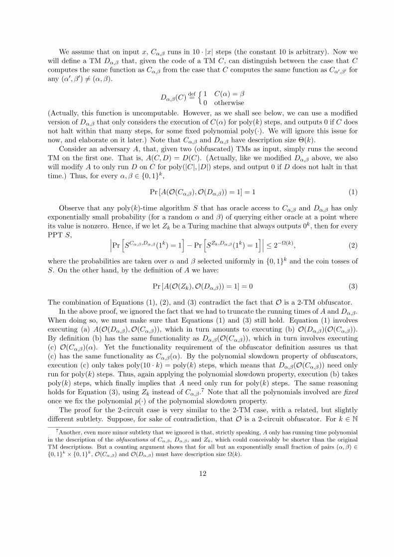
We assume that on input x, Cα,β runs in 10 · |x| steps (the constant 10 is arbitrary). Now wewill define a TM Dα,β that, given the code of a TM C, can distinguish between the case that Ccomputes the same function as Cα,β from the case that C computes the same function as Cα′,β′ forany (α′, β′) 6= (α, β).

Dα,β(C) def=

1 C(α) = β0 otherwise

(Actually, this function is uncomputable. However, as we shall see below, we can use a modifiedversion of Dα,β that only considers the execution of C(α) for poly(k) steps, and outputs 0 if C doesnot halt within that many steps, for some fixed polynomial poly(·). We will ignore this issue fornow, and elaborate on it later.) Note that Cα,β and Dα,β have description size Θ(k).

Consider an adversary A, that, given two (obfuscated) TMs as input, simply runs the secondTM on the first one. That is, A(C,D) = D(C). (Actually, like we modified Dα,β above, we alsowill modify A to only run D on C for poly(|C|, |D|) steps, and output 0 if D does not halt in thattime.) Thus, for every α, β ∈ 0, 1k,

Pr [A(O(Cα,β),O(Dα,β)) = 1] = 1 (1)

Observe that any poly(k)-time algorithm S that has oracle access to Cα,β and Dα,β has onlyexponentially small probability (for a random α and β) of querying either oracle at a point whereits value is nonzero. Hence, if we let Zk be a Turing machine that always outputs 0k, then for everyPPT S, ∣∣∣Pr

[SCα,β ,Dα,β (1k) = 1

]− Pr

[SZk,Dα,β (1k) = 1

]∣∣∣ ≤ 2−Ω(k), (2)

where the probabilities are taken over α and β selected uniformly in 0, 1k and the coin tosses ofS. On the other hand, by the definition of A we have:

Pr [A(O(Zk),O(Dα,β)) = 1] = 0 (3)

The combination of Equations (1), (2), and (3) contradict the fact that O is a 2-TM obfuscator.In the above proof, we ignored the fact that we had to truncate the running times of A and Dα,β.

When doing so, we must make sure that Equations (1) and (3) still hold. Equation (1) involvesexecuting (a) A(O(Dα,β),O(Cα,β)), which in turn amounts to executing (b) O(Dα,β)(O(Cα,β)).By definition (b) has the same functionality as Dα,β(O(Cα,β)), which in turn involves executing(c) O(Cα,β)(α). Yet the functionality requirement of the obfuscator definition assures us that(c) has the same functionality as Cα,β(α). By the polynomial slowdown property of obfuscators,execution (c) only takes poly(10 · k) = poly(k) steps, which means that Dα,β(O(Cα,β)) need onlyrun for poly(k) steps. Thus, again applying the polynomial slowdown property, execution (b) takespoly(k) steps, which finally implies that A need only run for poly(k) steps. The same reasoningholds for Equation (3), using Zk instead of Cα,β.7 Note that all the polynomials involved are fixedonce we fix the polynomial p(·) of the polynomial slowdown property.

The proof for the 2-circuit case is very similar to the 2-TM case, with a related, but slightlydifferent subtlety. Suppose, for sake of contradiction, that O is a 2-circuit obfuscator. For k ∈ N

7Another, even more minor subtlety that we ignored is that, strictly speaking, A only has running time polynomialin the description of the obfuscations of Cα,β , Dα,β , and Zk, which could conceivably be shorter than the originalTM descriptions. But a counting argument shows that for all but an exponentially small fraction of pairs (α, β) ∈0, 1k × 0, 1k, O(Cα,β) and O(Dα,β) must have description size Ω(k).

12

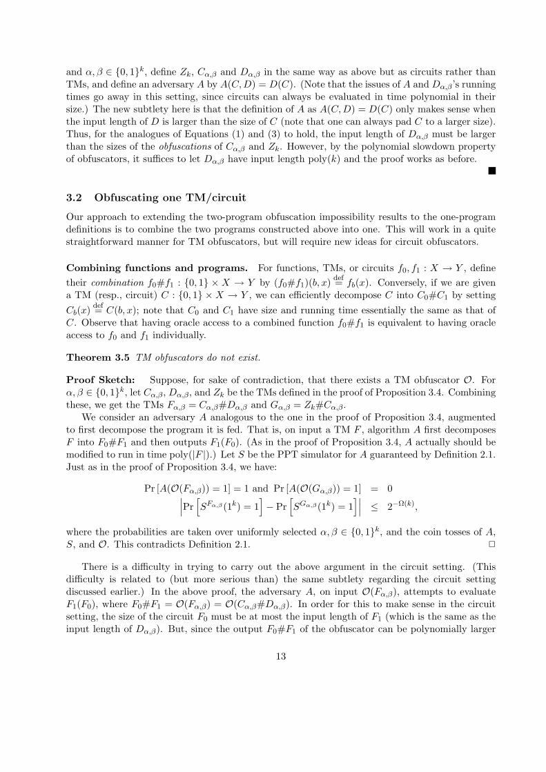
and α, β ∈ 0, 1k, define Zk, Cα,β and Dα,β in the same way as above but as circuits rather thanTMs, and define an adversary A by A(C,D) = D(C). (Note that the issues of A and Dα,β’s runningtimes go away in this setting, since circuits can always be evaluated in time polynomial in theirsize.) The new subtlety here is that the definition of A as A(C,D) = D(C) only makes sense whenthe input length of D is larger than the size of C (note that one can always pad C to a larger size).Thus, for the analogues of Equations (1) and (3) to hold, the input length of Dα,β must be largerthan the sizes of the obfuscations of Cα,β and Zk. However, by the polynomial slowdown propertyof obfuscators, it suffices to let Dα,β have input length poly(k) and the proof works as before.

3.2 Obfuscating one TM/circuit

Our approach to extending the two-program obfuscation impossibility results to the one-programdefinitions is to combine the two programs constructed above into one. This will work in a quitestraightforward manner for TM obfuscators, but will require new ideas for circuit obfuscators.

Combining functions and programs. For functions, TMs, or circuits f0, f1 : X → Y , definetheir combination f0#f1 : 0, 1 × X → Y by (f0#f1)(b, x) def= fb(x). Conversely, if we are givena TM (resp., circuit) C : 0, 1 ×X → Y , we can efficiently decompose C into C0#C1 by settingCb(x) def= C(b, x); note that C0 and C1 have size and running time essentially the same as that ofC. Observe that having oracle access to a combined function f0#f1 is equivalent to having oracleaccess to f0 and f1 individually.

Theorem 3.5 TM obfuscators do not exist.

Proof Sketch: Suppose, for sake of contradiction, that there exists a TM obfuscator O. Forα, β ∈ 0, 1k, let Cα,β, Dα,β, and Zk be the TMs defined in the proof of Proposition 3.4. Combiningthese, we get the TMs Fα,β = Cα,β#Dα,β and Gα,β = Zk#Cα,β.

We consider an adversary A analogous to the one in the proof of Proposition 3.4, augmentedto first decompose the program it is fed. That is, on input a TM F , algorithm A first decomposesF into F0#F1 and then outputs F1(F0). (As in the proof of Proposition 3.4, A actually should bemodified to run in time poly(|F |).) Let S be the PPT simulator for A guaranteed by Definition 2.1.Just as in the proof of Proposition 3.4, we have:

Pr [A(O(Fα,β)) = 1] = 1 and Pr [A(O(Gα,β)) = 1] = 0∣∣∣Pr[SFα,β (1k) = 1

]− Pr

[SGα,β (1k) = 1

]∣∣∣ ≤ 2−Ω(k),

where the probabilities are taken over uniformly selected α, β ∈ 0, 1k, and the coin tosses of A,S, and O. This contradicts Definition 2.1. 2

There is a difficulty in trying to carry out the above argument in the circuit setting. (Thisdifficulty is related to (but more serious than) the same subtlety regarding the circuit settingdiscussed earlier.) In the above proof, the adversary A, on input O(Fα,β), attempts to evaluateF1(F0), where F0#F1 = O(Fα,β) = O(Cα,β#Dα,β). In order for this to make sense in the circuitsetting, the size of the circuit F0 must be at most the input length of F1 (which is the same as theinput length of Dα,β). But, since the output F0#F1 of the obfuscator can be polynomially larger

13

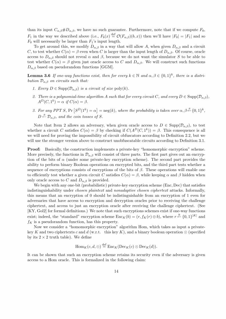
than its input Cα,β#Dα,β, we have no such guarantee. Furthermore, note that if we compute F0,

F1 in the way we described above (i.e., Fb(x) def= O(Fα,β)(b, x)) then we’ll have |F0| = |F1| and soF0 will necessarily be larger than F1’s input length.

To get around this, we modify Dα,β in a way that will allow A, when given Dα,β and a circuitC, to test whether C(α) = β even when C is larger than the input length of Dα,β. Of course, oracleaccess to Dα,β should not reveal α and β, because we do not want the simulator S to be able totest whether C(α) = β given just oracle access to C and Dα,β. We will construct such functionsDα,β based on pseudorandom functions [GGM].

Lemma 3.6 If one-way functions exist, then for every k ∈ N and α, β ∈ 0, 1k, there is a distri-bution Dα,β on circuits such that:

1. Every D ∈ Supp(Dα,β) is a circuit of size poly(k).

2. There is a polynomial-time algorithm A such that for every circuit C, and every D ∈ Supp(Dα,β),AD(C, 1k) = α if C(α) = β.

3. For any PPT S, Pr[SD(1k) = α

]= neg(k), where the probability is taken over α, β

R←0, 1k,D

R←Dα,β, and the coin tosses of S.

Note that Item 2 allows an adversary, when given oracle access to D ∈ Supp(Dα,β), to testwhether a circuit C satisfies C(α) = β by checking if C(AD(C, 1k)) = β. This consequence is allwe will need for proving the impossibility of circuit obfuscators according to Definition 2.2, but wewill use the stronger version above to construct unobfuscatable circuits according to Definition 3.1.

Proof: Basically, the construction implements a private-key “homomorphic encryption” scheme.More precisely, the functions in Dα,β will consist of three parts. The first part gives out an encryp-tion of the bits of α (under some private-key encryption scheme). The second part provides theability to perform binary Boolean operations on encrypted bits, and the third part tests whether asequence of encryptions consists of encryptions of the bits of β. These operations will enable oneto efficiently test whether a given circuit C satisfies C(α) = β, while keeping α and β hidden whenonly oracle access to C and Dα,β is provided.

We begin with any one-bit (probabilistic) private-key encryption scheme (Enc,Dec) that satisfiesindistinguishability under chosen plaintext and nonadaptive chosen ciphertext attacks. Informally,this means that an encryption of 0 should be indistinguishable from an encryption of 1 even foradversaries that have access to encryption and decryption oracles prior to receiving the challengeciphertext, and access to just an encryption oracle after receiving the challenge ciphertext. (See[KY, Gol2] for formal definitions.) We note that such encryptions schemes exist if one-way functionsexist; indeed, the “standard” encryption scheme EncK(b) = (r, fK(r)⊕ b), where r

R←0, 1|K| andfK is a pseudorandom function, has this property.

Now we consider a “homomorphic encryption” algorithm Hom, which takes as input a private-key K and two ciphertexts c and d (w.r.t. this key K), and a binary boolean operation (specifiedby its 2× 2 truth table). We define

HomK(c, d,) def= EncK(DecK(c)DecK(d)).

It can be shown that such an encryption scheme retains its security even if the adversary is givenaccess to a Hom oracle. This is formalized in the following claim:

14

Claim 3.7 For every PPT A,∣∣Pr[AHomK ,EncK (EncK(0)) = 1

]− Pr

[AHomK ,EncK (EncK(1)) = 1

]∣∣ ≤ neg(k).

Proof of claim: Suppose there were a PPT A violating the claim. First, we argue thatwe can replace the responses to all of A’s HomK-oracle queries with encryptions of 0 withonly a negligible effect on A’s distinguishing gap. This follows from indistinguishabilityunder chosen plaintext and ciphertext attacks and a hybrid argument: Consider hybridswhere the first i oracle queries are answered according to HomK and the rest withencryptions of 0. Any advantage in distinguishing two adjacent hybrids must be due todistinguishing an encryption of 1 from an encryption of 0. The resulting distinguishercan be implemented using oracle access to encryption and decryption oracles prior toreceiving the challenge ciphertext (and an encryption oracle afterward).

Once we have replaced the HomK-oracle responses with encryptions of 0, we have anadversary that can distinguish an encryption of 0 from an encryption of 1 when givenaccess to just an encryption oracle. This contradicts indistinguishability under chosenplaintext attack. 2

Now we return to the construction of our circuit family Dα,β. For a key K, let EK,α be analgorithm that, on input i outputs EncK(αi), where αi is the i’th bit of α. Let BK,α,β be analgorithm that when fed a k-tuple of ciphertexts (c1, . . . , ck) outputs α if for all i, DecK(ci) = βi,where β1, . . . , βk are the bits of β. A random circuit from Dα,β will essentially be the algorithm

DK,α,βdef= EK,α#HomK#BK,α,β

(for a uniformly selected key K). One minor complication is that DK,α,β is actually a probabilisticalgorithm, since EK,α and HomK employ probabilistic encryption, whereas the lemma requiresdeterministic functions. This can be solved in the usual way, by using pseudorandom functions.Let q = q(k) be the input length of DK,α,β and m = m(k) the maximum number of random bitsused by DK,α,β on any input. We can select a pseudorandom function fK′ : 0, 1q → 0, 1m, andlet D′K,α,β,K′ be the (deterministic) algorithm, that on input x ∈ 0, 1q evaluates DK,α,β(x) usingrandomness fK′(x).

Define the distribution Dα,β to be D′K,α,β,K′ , over uniformly selected keys K and K ′. We arguethat this distribution has the properties stated in the lemma. By construction, each D′K,α,β,K′ iscomputable by circuit of size poly(k), so Property 1 is satisfied.

For Property 2, consider an algorithm A that on input C and oracle access to D′K,α,β,K′ (which,as usual, we can view as access to (deterministic versions of) the three separate oracles EK,α,HomK , and BK,α,β), proceeds as follows: First, with k oracle queries to the EK,α oracle, A obtainsencryptions of each of the bits of α. Then, A uses the HomK oracle to do a gate-by-gate emulationof the computation of C(α), in which A obtains encryptions of the values at each gate of C. Inparticular, A obtains encryptions of the values at each output gate of C (on input α). It then feedsthese output encryptions to DK,α,β , and outputs the response to this oracle query. By construction,A outputs α if C(α) = β.

Finally, we verify Property 3. Let S be any PPT algorithm. We must show that S has only anegligible probability of outputting α when given oracle access to D′K,α,β,K′ (over the choice of K,α, β, K ′, and the coin tosses of S). By the pseudorandomness of fK′ , we can replace oracle access to

15

the function D′K,α,β,K′ with oracle access to the probabilistic algorithm DK,α,β with only a negligibleeffect on S’s success probability. Oracle access to DK,α,β is equivalent to oracle access to EK,α,HomK , and BK,α,β . Since β is independent of α and K, the probability that S queries BK,α,β at apoint where its value is nonzero (i.e., at a sequence of encryptions of the bits of β) is exponentiallysmall, so we can remove S’s queries to BK,α,β with only a negligible effect on the success probability.Oracle access to EK,α is equivalent to giving S polynomially many encryptions of each of the bitsof α. Thus, we must argue that S cannot compute α with nonnegligible probability from theseencryptions and oracle access to HomK . This follows from the fact that the encryption schemeremains secure in the presence of a HomK oracle (Claim 3.7) and a hybrid argument.

Now we can prove the impossibility of circuit obfuscators.

Theorem 3.8 If one-way functions exist, then circuit obfuscators do not exist.

Proof: Suppose, for sake of contradiction, that there exists a circuit obfuscator O. For k ∈ Nand α, β ∈ 0, 1k, let Zk and Cα,β be the circuits defined in the proof of Proposition 3.4, and letDα,β be the distribution on circuits given by Lemma 3.6. For each k ∈ N, consider the followingtwo distributions on circuits of size poly(k):

Fk: Choose α and β uniformly in 0, 1k, DR←Dα,β. Output Cα,β#D.

Gk: Choose α and β uniformly in 0, 1k, DR←Dα,β. Output Zk#D.

Let A be the PPT algorithm guaranteed by Property 2 in Lemma 3.6, and consider a PPT A′

that, on input a circuit F , decomposes F = F0#F1 and outputs 1 if F1(AF1(F0, 1k)) = β, wherek is the input length of F0. Thus, when fed a circuit from O(Fk) (resp., O(Gk)), A′ is evaluatingC(AD(C, 1k)) where D computes the same function as some circuit from Dα,β and C computes thesame function as Cα,β (resp., Zk). Therefore, by Property 2 in Lemma 3.6, we have:

Pr[A′(O(Fk)) = 1

]= 1, and

Pr[A′(O(Gk)) = 1

]= 0.

We now argue that for any PPT algorithm S∣∣∣Pr[SFk(1k) = 1

]− Pr

[SGk(1k) = 1

]∣∣∣ ≤ 2−Ω(k),

which will contradict the definition of circuit obfuscators. Having oracle access to a circuit fromFk (respectively, Gk) is equivalent to having oracle access to Cα,β (resp., Zk) and D

R←Dα,β, whereα, β are selected uniformly in 0, 1k. Property 3 of Lemma 3.6 implies that the probability thatS queries the first oracle at α is negligible, and hence S cannot distinguish that oracle being Cα,β

from it being Zk.

We can remove the assumption that one-way functions exist for efficient circuit obfuscators viathe following (easy) lemma.

Lemma 3.9 If efficient obfuscators exist, then one-way functions exist.

16

Proof Sketch: Suppose that O is an efficient obfuscator as per Definition 2.2. For α ∈ 0, 1kand b ∈ 0, 1, let Cα,b : 0, 1k → 0, 1 be the circuit defined by

Cα,b(x) def=

b x = α0 otherwise.

Now define fk(α, b, r) def= O(Cα,b; r), i.e. the obfuscation of Cα,b using coin tosses r. We will arguethat f =

⋃k∈N fk is a one-way function. Clearly fk can be evaluated in time poly(k). Since the

bit b is information-theoretically determined by fk(α, b, r), to show that f is one-way it suffices toshow that b is a hardcore bit of f . To prove this, we first observe that for any PPT S,

Prα,b

[SCα,b(1k) = b

]≤ 1

2+ neg(k).

By the virtual black box property of O, it follows that for any PPT A,

Prα,b,r

[A(f(α, b, r)) = b] = Prα,b,r

[A(O(Cα,b; r)) = b] ≤ 12

+ neg(k).

This demonstrates that b is indeed a hard-core bit of f , and hence that f is one-way. 2

Corollary 3.10 Efficient circuit obfuscators do not exist (unconditionally).

We now strengthen our result to not only rule out circuit obfuscators, but actually yield unob-fuscatable programs.

Theorem 3.11 (unobfuscatable programs) If one-way functions exist, then there exists a un-obfuscatable circuit ensemble.

Proof: Our unobfuscatable circuit ensemble Hk is defined as follows.

Hk: Choose α, β, γ uniformly in 0, 1k, DR←Dα,β. Output Cα,β#D#Cα,(D,γ).8

(Above, Cα,(D,γ) is the circuit that on input α outputs (D, γ), and on all other inputs outputs0|(D,γ)|.)

Efficiency is clearly satisfied. For unobfuscatability, we define π(Cα,β#D#Cα,(D,γ)) = γ. Let’sverify that γ is pseudorandom given oracle access. That is, for every PPT S,∣∣∣∣∣ Pr

CR←Hk

[SC(π(C)) = 1]− PrC

R←Hk,zR←0,1k

[SC(z) = 1]

∣∣∣∣∣ ≤ neg(k)

Having oracle access to a circuit from Hk is equivalent to having oracle access to Cα,β, Cα,(D,γ), andD

R←Dα,β, where α, β, and γ are selected uniformly in 0, 1k. Property 3 of Lemma 3.6 impliesthat the probability that any PPT S queries either of the Cα,·-oracles at α and thus gets a nonzeroresponse is negligible. Note that this holds even if the PPT S is given γ as input, because the

8Actually it would be equivalent to use Cα,(β,D,γ)#D, but it will be notationally convenient in the proof to splitthe C circuit into two parts.

17

probabilities in Lemma 3.6 are taken over only α, β, and DR←Dα,β, so we can view S as choosing

γ on its own. Thus,

Prf

R←Hk

[Sf (π(f)) = 1] = Prα,β,γ

R←0,1k,DR←Dα,β

[SCα,β#D#Cα,(D,γ)(γ) = 1]

= Prα,β,γ,γ′

R←0,1k,DR←Dα,β

[SCα,β#D#Cα,(D,γ′)(γ) = 1]± neg(k)

= Prf

R←Hk,zR←0,1k

[Sf (z) = 1]± neg(k).

Finally, let’s show that given any circuit C ′ computing the same function as Cα,β#D#Cα,(D,γ),we can reconstruct the latter circuit. First, we can decompose C ′ = C1#D′#C2. Since D′ computesthe same function as D and C1(α) = β, we have AD′

(C1) = α, where A is the algorithm fromProperty 2 of Lemma 3.6. Given α, we can obtain β = C1(α) and (D, γ) = C2(α), which allows usto reconstruct Cα,β#D#Cα,(D,γ).

4 Extensions

4.1 Approximate obfuscators

One of the most reasonable ways to weaken the definition of obfuscators, is to relax the conditionthat the obfuscated circuit must compute exactly the same function as the original circuit. Rather,we can allow the obfuscated circuit to only approximate the original circuit.

We must be careful in defining “approximation”. We do not want to lose the notion of anobfuscator as a general purpose scrambling algorithm and therefore we want a definition of approx-imation that will be strong enough to guarantee that the obfuscated circuit can still be used inthe place of the original circuit in any application. Consider the case of a signature verificationalgorithm VK . A polynomial-time algorithm cannot find an input on which VK does not output0 (without knowing the signature key). However, we clearly do not want this to mean that theconstant zero function is an approximation of VK .

4.1.1 Definition and Impossibility Result

In order to avoid the above pitfalls we choose a definition of approximation that allows the obfus-cated circuit to deviate on a particular input from the original circuit only with negligible probabilityand allows this event to depend on only the coin tosses of the obfuscating algorithm (rather thanover the choice of a randomly chosen input).

Definition 4.1 For any function f : 0, 1n → 0, 1k, ε > 0, the random variable D is called anε-approximate implementation of f if the following holds:

1. D ranges over circuits from 0, 1n to 0, 1k

2. For any x ∈ 0, 1n , PrD[D(x) = f(x)] ≥ 1− ε

We then define a strongly unobfuscatable circuit ensemble to be an unobfuscatable circuitensemble where the original circuit C can be reconstructed not only from any circuit that computesthe same function as C but also from any approximate implementation of C.

18

Definition 4.2 A strongly unobfuscatable circuit ensemble Hkk∈N is defined in the same wayas an unobfuscatable condition ensemble, except that Part 2 of the “unobfuscatability” condition isstrengthened as follows:

2. C is easy to reconstruct given an approximate implementation: There exists a PPT A and apolynomial p(·) such that for every C ∈

⋃k∈N Supp(Hk) and for any random variable C ′ that

is an ε-approximate implementation of the function computed by C

Pr[A(C ′) = C] ≥ 1− ε · p(k)

Our main theorem in this section is the following:

Theorem 4.3 If one-way functions exist, then there exists a strongly unobfuscatable circuit en-semble.

Similarly to the way that Theorem 3.11 implies Theorem 3.8, Theorem 4.3 implies that, assum-ing the existence of one-way functions, an even weaker definition of circuit obfuscators (one thatallows the obfuscated circuit to only approximate the original circuit) is impossible to meet. Wenote that it some (but not all) applications of obfuscators, a weaker notion of approximation mightsuffice. Specifically, in some cases it suffices for the obfuscator to only approximately preservefunctionality with respect to a particular distribution on inputs, such as the uniform distribution.(This is implied, but apparently weaker, than the requirement of Definition 4.1 — if C is an ε-approximate implementation of f , then for any fixed distribution D on inputs, C and f agree ona 1 −

√ε fraction of D with probability at least 1 −

√ε.) We do not know whether approximate

obfuscators with respect to this weaker notion exist, and leave it as an open problem.We shall prove this theorem in the following stages. First we will see why the proof of Theo-

rem 3.11 does not apply directly to the case of approximate implementations. Then we shall definea construct called invoker-randomizable pseudorandom functions, which will help us modify theoriginal proof to hold in this case.

4.1.2 Generalizing the Proof of Theorem 3.11 to the Approximate Case

The first question is whether the proof of Theorem 3.11 already shows that the ensemble Hkk∈Ndefined there is actually a strongly unobfuscatable circuit ensemble. As we explain below, theanswer is no.

To see why, let us recall the definition of the ensemble Hkk∈N that is defined there. Thedistribution Hk The distribution Hk is defined by choosing α, β, γ

R←0, 1k , a function DR←Dα,β

and outputting Cα,β#D#Cα,(D,γ).That proof gave an algorithm A′ that reconstructs C ∈ H given any circuit that computes

exactly the same function as C. Let us see why A′ might fail when given only an approximateimplementation of C. On input a circuit F , A′ works as follows: It decomposes F into two circuitsF = F1#F2#F3. F2 and F3 are used only in a black-box manner, but the queries A′ makes toF2 depend on the gate structure of the circuit F1. The problem is that a vicious approximateimplementation for a function Cα,β#D#Cα,(D,γ) ∈ Supp(Hk) may work in the following way:choose a random circuit F1 out of some set C of exponentially many circuits that compute Cα,β,take F2 that computes D, and F3 that computes Cα,(D,γ). Then see at which points A′ queries

19

F2 when given F1#F2#F3 as input.9 As these places depend on F1, it is possible that for eachF1 ∈ C, there is a point x(F1) such that A′ will query F2 at the point x(F1), but x(F1) 6= x(F ′1) forany F ′1 ∈ C \ F1. If the approximate implementation changes the value of F2 at x(F1), then A′’scomputation on F1#F2#F3 is corrupted.

One way to solve this problem would be to make the queries that A′ makes to F2 independent ofthe structure of F1. (This already holds for F3, which is only queried at α in a correct computation.)If A′ had this property, then given an ε-approximate implementation of Cα,β#D#Cα,(D,γ), eachquery of A′ would have only an ε chance to get an incorrect answer and overall A′ would succeedwith probability 1−ε ·p(k) for some polynomial p(·). (Note that the probability that F1(α) changesis at most ε.)

We will not be able to achieve this, but something slightly weaker that still suffices. Let’s lookmore closely at the structure of Dα,β that is defined in the proof of Lemma 3.6. We defined therethe algorithm

DK,α,βdef= EK,α#HomK#BK,α,β

and turned it into a deterministic function by using a pseudorandom function f ′K and definingD′K,α,β,K′ to be the deterministic algorithm that on input x ∈ 0, 1q evaluates DK,α,β(x) us-ing randomness fK′(x). We then defined Dα,β to be D′K,α,β,K′ = E′K,α,K′#Hom′K,K′#BK,α,β foruniformly selected private key K and seed K ′.

Now our algorithm A′ (that uses the algorithm A defined in Lemma 3.6) treats F2 as threeoracles: E, H, and B , where if F2 computes D = E′K,α,K′#Hom′K,K′#BK,α,β then E is the oracleto E′K,α,K′ , H is the oracle to Hom′K,K′ and B is the oracle to BK,α,β . The queries to E are at theplaces 1, . . . , k and so are independent of the structure of F1. The queries that A makes to the Horacle, however, do depend on the structure of F1.

Recall that any query A′ makes to the H oracle are of the form (c, d,) where c and d areciphertexts of some bits, and is a 4-bit description of a binary boolean function. Just formotivation, suppose that A′ has the following ability: given an encryption c, A′ can generate arandom encryption of the same bit (i.e., distributed according to EncK(DecK(c), r) for uniformlyselected r). For instance, this would be true if the encryption scheme were “random self-reducible.”Suppose now that, before querying the H oracle with (c, d,), A′ generates c′, d′ that are randomencryptions of the same bits as c, d and query the oracle with (c′, d′,) instead. We claim thatif F2 is an ε-approximate implementation of D, then for any such query, there is at most a 64εprobability for the answer to be wrong even if (c, d,) depend on the circuit F . The reason is thatthe distribution of the modified query (c′, d′,) depends only on (DecK(c),DecK(d),), and thereare only 2 · 2 · 24 = 64 possibilities for the latter. For each of the 64 possibilities, the probabilityof an incorrect answer (over the choice of F ) is at most ε. Choosing (DecK(c),DecK(d),) after Fto maximize the probability of an incorrect answer multiplies this probability by at most 64.

We shall now use this motivation to fix the function D so that A′ will essentially have thisdesired ability of randomly self-reducing any encryption to a random encryption of the same bit.Recall that Hom′K,K′(c, d,) = EncK(DecK(c)DecK(d); fK′(c, d,)). Now, a naive approach toensure that any query returns a random encryption of DecK(c)DecK(d) would be to change thedefinition of Hom′ to the following: Hom′K,K′(c, d,, r) = EncK(DecK(c) DecK(d); r). Then wechange A′ to an algorithm A′′ that chooses a uniform r ∈ 0, 1n and thereby ensures that the

9Recall that A′ is not some given algorithm that we must treat as a black-box but rather a specific algorithm thatwe defined ourselves.

20

result is a random encryption of DecK(c)DecK(d). The problem is that this construction wouldno longer satisfy Property 3 of Lemma 3.6 (security against a simulator with oracle access). Thisis because the simulator could now control the random coins of the encryption scheme and use thisto break it. Our solution will be to redefine Hom′ in the following way:

Hom′K,K′(c, d,, r) = EncK(DecK(c)DecK(d); fK′(c, d,, r))

but require an additional special property from the pseudorandom function fK′ .

4.1.3 Invoker-Randomizable Pseudorandom Functions

The property we would like the pseudorandom function fK′ to possess is the following:

Definition 4.4 A function ensemble fK′K′∈0,1∗ (fK′ : 0, 1q+n → 0, 1n , where n and q arepolynomially related to |K ′|) is called an invoker-randomizable pseudorandom function ensemble ifthe following holds:

1. fK′K′∈0,1∗ is a pseudorandom function ensemble

2. For any x ∈ 0, 1q , if r is chosen uniformly in 0, 1n then fK′(x, r) is distributed uniformly(and so independently of x) in 0, 1n.

Fortunately, we can prove the following lemma:

Lemma 4.5 If pseudorandom functions exist then there exist invoker-randomizable pseudorandomfunctions.

Proof Sketch: Suppose that gK′K′∈0,1∗ is a pseudorandom function ensemble and thatpSS∈0,1∗ is a pseudorandom function ensemble in which for any S ∈ 0, 1∗ , pS is a permutation(the existence of such ensembles is implied by the existence of ordinary pseudorandom functionensembles [LR]).

We define the function ensemble fK′K′∈0,1∗ in the following way:

fK′(x, r) def= pgK′ (x)(r)

It is clear that this ensemble satisfies Property 2 of Definition 4.4 as for any x, the functionr 7→ fK′(x, r) is a permutation.

What needs to be shown is that it is a pseudorandom function ensemble. We do this by showingthat for any PPT D, the following probabilities are identical up to a negligible term.

1. PrK′ [DfK′ (1k) = 1] (where k = |K ′|).

2. PrG[D(x,R) 7→pG(x)(R)(1k) = 1], where G is a true random function.

3. PrP1,...,Pt [DP1,...,Pt(1k) = 1], where t = t(k) is a bound on the number of queries that D makesand each time D makes a query with a new value of x we use a new random function Pi.(This requires a hybrid argument).

4. PrF [DF (1k) = 1], where F is a truly random function.

2

21

4.1.4 Finishing the Proof of Theorem 4.3

Now, suppose we use a pseudorandom function fK′ that is invoker-randomizable, and modify thealgorithm A′ so that all its queries (c, d,) to the H oracle are augmented to be of the form(c, d,, r), where r is chosen uniformly and independently for each query. Then the result of eachsuch query is a random encryption of DecK(c)DecK(d). Therefore, as argued above, A′ never getsa wrong answer from the H oracle with probability at least 1− p(k) · ε, for some polynomial p(·).Indeed, this holds because aside from the first queries which are fixed and therefore independentof the gate structure of F1, all other queries are of the form (c, d,, r) where c and d are uniformlydistributed and independent encryptions of some bits a and b, and r is uniformly distributed. Only(a, b,) depend on the gate structure of F1, and there are only 64 possibilities for them. AssumingA′ never gets an incorrect answer from the H oracle, its last query to the B oracle will be auniformly distributed encryption of β1, . . . , βk, which is independent of the structure of F1, and sohas only an ε probability to be incorrect. This completes the proof.

One point to note is that we have converted our deterministic algorithm A′ of Theorem 3.11into a probabilistic algorithm.

4.2 Impossibility of the applications

So far, we have only proved impossibility of some natural and arguably minimalistic definitions forobfuscation. Yet it might seem that there’s still hope for a different definition of obfuscation, onethat will not be impossible to meet but would still be useful for some intended applications. We’llshow now that this is not the case for many of the applications we described in the introduction.Rather, any definition of obfuscator that would be strong enough to provide them, will be impossibleto meet.

Note that we do not prove that the applications themselves are impossible to meet, but ratherthat there does not exist an obfuscator (i.e., an algorithm satisfying the syntactic requirements ofDefinition 2.2) that can be used to achieve them in the ways that are described in Section 1.1. Ourresults in the section also extend to approximate obfuscators.

Consider, for example, the application to transforming private-key encryption to public-keyones. The circuit Ek in the following definition can be viewed as an encryption-key in the corre-sponding public-key encryption scheme.

Definition 4.6 A private-key encryption scheme (G, E,D) is called unobfuscatable if there existsa PPT A such that

PrK

R←G(1k)

[A(EK) = K] ≥ 1− neg(k)

where EK is any circuit that computes the encryption function with private key K.

Note that an unobfuscatable encryption scheme is unobfuscatable in a very strong sense. Anadversary is able to completely break the system given any circuit that computes the encryptionalgorithm.

We prove in Theorem 4.10 that if encryption schemes exist, then so do unobfuscatable encryp-tion schemes that satisfy the same security requirements.10 This means that any definition of an

10Recall that, for simplicity, we only consider deterministic encryption schemes here and relaxed notions of securitythat are consistent with them (cf., Footnote 2).

22

obfuscators that will be strong enough to allow the conversion of private-key encryption schemesinto public-key encryption schemes mentioned in Section 1.1, would be impossible to meet (becausethere exist unobfuscatable encryption schemes). Of course, this does not mean that public-key en-cryption schemes do not exist, nor that there do not exist private-key encryption schemes whereone can give the adversary a circuit that computes the encryption algorithm without loss of security(indeed, any public-key encryption scheme is in particular such a private-key encryption). Whatthis means is that there exists no general purpose way to transform a private key encryption schemeinto a public key encryption by obfuscating the encryption algorithm.

We present analogous definitions for unobfuscatable signature schemes, MACs, and pseudoran-dom functions.

Definition 4.7 A signature scheme (G, S, V ) is called unobfuscatable if there exists a PPT A suchthat

Pr(SK ,VK )

R←G(1k)

[A(SSK ) = SK ] ≥ 1− neg(k)

where SSK is any circuit that computes the signature function with signing key SK .

Definition 4.8 A message authentication scheme (G, S, V ) is called unobfuscatable if there existsa PPT A such that

PrK

R←G(1k)

[A(SK) = K] ≥ 1− neg(k)

where SK is any circuit that computes the tagging function with tagging key K.

Definition 4.9 A pseudorandom function ensemble hKK∈0,1∗ is called unobfuscatable if thereexists a p.p.t A such that

PrK

R←0,1k[A(HK) = K] ≥ 1− neg(k)

where HK is any circuit that computes hK .

One implication of the existence of unobfuscatable pseudorandom function ensembles is thatfor many natural protocols that are secure in the random oracle model (such as the Fiat–Shamirauthentication protocol [FS]), one can find a pseudorandom function ensemble hkk∈0,1∗ suchthat if the random oracle is replaced with any circuit that computes hk, the protocol would not besecure.

Theorem 4.10 1. If signature schemes exist, then so do unobfuscatable signature schemes.

2. If private-key encryption schemes exist, then so do unobfuscatable encryption schemes.

3. If pseudorandom function ensembles exist, then so do unobfuscatable pseudorandom functionensembles.

4. If message authentication schemes exist, then so do unobfuscatable message authenticationschemes.

23

Proof Sketch: First note that the existence of any one of these primitives implies the existence ofone-way functions [IL]. Therefore, Theorem 3.11 gives us a totally unobfuscatable circuit ensembleH = Hk.

Now, we shall sketch the construction of the unobfuscatable signature scheme. All other con-structions are similar. Take an existing signature scheme (G, S, V ) (where G is the key generationalgorithm, S the signing algorithm, and V the verification algorithm). Define the new scheme(G′, S′, V ′) as follows:

The generator G′ on input 1k uses the generator G to generate signing and verifying keys(SK ,VK ) R←G(1k). It then samples a circuit C

R←H`, where ` = |SK |. The new signing key SK ′

is (SK , C) while the verification key VK ′ is the same as VK .We can now define

S′SK ,f (m) def= (SSK (m), C(m),SK ⊕ π(C)),

where π is the function from the unobfuscatability condition in Definition 3.1.

V ′VK (m, (τ, x)) def= VVK (m, τ)

We claim that (G′, S′, V ′) is an unobfuscatable, yet secure, signature scheme. Clearly, given anycircuit that computes S′SK ,f , one can obtain SK ⊕ π(C) and a circuit that computes the samefunction as C. Possession of the latter enables one to reconstruct the original circuit C itself, fromwhich π(C) and then SK can be computed.

To see that scheme (G′, S′, V ′) retains the security of the scheme (G, S, V ), observe that beinggiven oracle access to S′SK ,C is equivalent to being given oracle access to SSK and C, along withbeing given the string π(C) ⊕ SK . Using the facts that π(C) is indistinguishable from randomgiven oracle access to C and that C is chosen independently of SK , it can be easily shown that thepresence of C and π(C)⊕ SK does not help an adversary break the signature scheme.

The constructions of the unobfuscatable encryption scheme and pseudorandom function ensem-ble are similar. The only detail is that when we construct the pseudorandom function ensemble, weneed to observe that Theorem 3.11 can be modified to give H that is also a family of pseudorandomfunctions. (To do this, all places where the functions C in H were defined to be zero should insteadbe replaced with values of a pseudorandom function.) 2

4.3 Obfuscating restricted circuit classes

Given our impossibility results for obfuscating general circuits, one may ask whether it is easier toobfuscate computationally restricted classes of circuits. Here we argue that this is unlikely for allbut very weak models of computation.

Theorem 4.11 If factoring Blum integers is “hard”11 then there is a family Hk of unobfuscatablecircuits such that every C

R←Hk is a constant-depth threshold circuit of size poly(k) (i.e., in TC0).

Proof Sketch: Naor and Reingold [NR] showed that under the stated assumptions, there exists afamily of pseudorandom functions computable in TC0. Thus, we simply need to check that we canbuild our unobfuscatable circuits from such a family without a substantial increase in depth. Recallthat the unobfuscatable circuit ensemble Hk constructed in the proof of Theorem 3.11 consists of

11This result is also implied if the Decisional Diffie–Hellman problem is “hard”; see [NR] for precise statements ofthese assumptions.

24

functions of the form Cα,β#D#Cα,(D,γ), where D is from the family Dα,β of Lemma 3.6. It is easy tosee that Cα,β and Cα,(D,γ) are in TC0, so we only need to check that Dα,β consists of circuits in TC0.The computational complexity of circuits in the family Dα,β is dominated by performing encryptionsand decryptions in a private-key encryption scheme (Enc,Dec) and evaluating a pseudorandomfunction fK′ that is used to derandomize the probabilistic circuit DK,α,β . If we use the Naor–Reingold pseudorandom functions both for fK′ and to construct the encryption scheme (in theusual way, setting EncK(b) = (r, fK(r)⊕ b)), then the resulting circuit is in TC0. 2

4.4 Relativization

In this section, we discuss whether our results relativize. To do this, we must clarify the definitionof an obfuscator relative to an oracle F : 0, 1∗ → 0, 1∗. What we mean is that all algorithms inthe definition, including the one being obfuscated and including the adversary, have oracle accessto F . For a circuit, this means that the circuit can have gates for evaluating F . We fix an encodingof (oracle) circuits as binary strings such that a circuit described by a string of length s can onlymake oracle queries of total length at most s.

By inspection, our initial (easy) impossibility results hold relative to any oracle, as they involveonly simulation and diagonalization.

Proposition 4.12 Proposition 3.4 (impossibility of 2-circuit obfuscators) and Theorem 3.5 (im-possibility of TM obfuscators) hold relative to any oracle.

Interestingly, however, our main impossibility results do not relativize.

Proposition 4.13 There is an oracle relative to which efficient circuit obfuscators exist. Thus,Theorem 3.8, Theorem 3.11, and Corollary 3.10 do not relativize.

This can be viewed both as evidence that these results are nontrivial, and as (further) evidencethat relativization is not a good indication of what we can prove.

Proof Sketch: The oracle F =⋃

k Fk will consist of two parts Fk = Ok#Ek, where Ok :0, 1k×0, 1k → 0, 16k, and Ek : 0, 16k×0, 1k → 0, 1k. Ok is simply a uniformly randominjective function of the given parameters. Ek(x, y) is defined as follows: If there exists a (C, r)such that Ok(C, r) = x, then Ek(x, y) = CF (y) (where C is viewed as the description of a circuit).Otherwise, Ek(x, y) = ⊥. Note that this definition of Fk is not circular, because C can only makeoracle queries of size at most |C| = k, and hence can only query Fk′ for k′ ≤ k/2.

Now we can view x = Ok(C, r) as an obfuscation of C using coin tosses r. This satisfiesthe syntactic requirements of obfuscation, since |x| = O(|C|) and the Ek allows one to efficientlyevaluate C(y) given just x and y. (Technically, we should define the obfuscation of C to be a circuitthat has x hardwired in and makes an oracle query to Ek.)

So we only need to prove the virtual black-box property. By a union bound over polynomial-time adversaries A of description size smaller than k/2 and circuits C of size k, it suffices to provethe following claim.12

12Note that we are only proving the virtual black-box property against adversaries of “bounded nonuniformity,”which in particular includes all uniform PPT adversaries. Presumably it can also be proven against nonuniformadversaries, but we stick to uniform adversaries for simplicity.

25

Claim 4.14 For every PPT A there exists a PPT S such that for every circuit C of size k, thefollowing holds with probability at least 1− 2−2k over F :∣∣∣∣∣ Pr

rR←0,1k

[AF (Ok(C, r)) = 1

]− Pr

[SF,C(1k) = 1

]∣∣∣∣∣ ≤ 2−Ω(k)

Fix a PPT A. We define the simulator S as follows. SF,C(1k) chooses xR←0, 16k and simulates

AF (x), using its own F -oracle to answer A’s oracle queries, except A’s queries to Ek′ for k′ ≥ k.On A’s query (x′, y′) to Ek′ , S feeds A the response z computed as follows:

1. If x′ = x, then set z = C(y′) (computed using oracle access to C).

2. Else if x′ = Ok′(C ′, r′) for some previous query (C ′, r′) to the Ok′-oracle, then set z =(C ′)F (y′) (computed recursively using these same rules).

3. Else set z = ⊥.

From the fact that a circuit of size s can only make oracle queries of total length s, it follows thatthe recursive evaluation of (C ′)F (y) only incurs a polynomial overhead in running time. Also notethat S never queries the Ek′ oracle for k′ ≥ k.

Let us denote the execution of the above simulation for a particular x by SF,C(x). Notice thatwhen x = Ok(C, r) for some r, then SF,C(x) and AF (x) have exactly the same behavior unlessthe above simulation produces some query (x′, y′) such that x′ ∈ Image(Ok′), x′ 6= x, and x′ wasnot obtained by a previous query to Ok′ . Since O is a random length-tripling function, it followsthat the latter happens with probability at most poly(k) · 22k/26k, taken over the choice of F anda random r (recall that x = Ok(C, r)).13 Thus, with probability at least 1 − 2−3k over the choiceof F , SF,C(Ok(C, r)) = AF (Ok(C, r)) for all but a 2−Ω(k) fraction of r’s.

Thus, proving Claim 4.14 reduces to showing that:∣∣∣∣∣ Prr

R←0,1k

[SF,C(Ok(C, r)) = 1

]− Pr

xR←0,16k

[SF,C(x) = 1

]∣∣∣∣∣ ≤ 2−Ω(k)

with high probability (say, 1− 23k) over the choice of F .In other words, we need to show that the function G(r)def=Ok(C, r) is a pseudorandom generator

against S. Since G is a random function from 0, 1k → 0, 16k, this would be obvious were it notfor the fact that S has oracle access to F (which is correlated with G). Recall, however, that wemade sure that S does not query the Ek′-oracle for any k′ ≥ k. This enables us to use the followinglemma, proven in Appendix B.

Lemma 4.15 There is a constant δ > 0 such that the following holds for all sufficiently large Kand any L ≥ K2. Let D be an algorithm that makes at most Kδ oracle queries and let G be arandom injective function G : [K]→ [L]. Then with probability at least 1− 2−Kδ

over G,∣∣∣∣ Prx∈[K]

[DG(G(x)) = 1

]− Pr

y∈[L]

[DG(y) = 1

]∣∣∣∣ ≤ 1Kδ

.

13Technically, this probability (and later ones in the proof) should also be taken over the coin tosses of A/S.

26

Let us see how Lemma 4.15 implies what we want. Let K = 2k and associate [K] with 0, 1k.We fix all values of Ok′ for all k′ 6= k and Ek′ for all k′ < k. We also fix the values of Ok(C ′, r) forall C ′ 6= C, and view G(r) def= Ok(C, r) as a random injective function from [K] to the remainingL = K6−(K−1)·K elements of 0, 16k. The only oracle queries of S that vary with the choice of Gare queries to Ok at points of the form (C, r), which is equivalent to queries to G. Thus, Lemma 4.15implies that the output of G is indistinguishable from the uniform distribution on some subset of0, 16k of size L. Since the latter has statistical difference (K6−L)/K6 < 1/K4 from the uniformdistribution on 0, 16k, we conclude that G is ε-pseudorandom (for ε = 1/Kδ + 1/K4 = 2−Ω(k))against S with probability at least 1− 2−Kδ

> 1− 2−3k, as desired. 2

While our result does not relativize in the usual sense, the proof does work for a slightly differentform of relativization, which we refer to as bounded relativization (and reflects how the RandomOracle Model is sometimes interpreted in cryptography.) In bounded relativization, an oracle isa finite function with fixed input length (polynomially related to the security parameter k), andall algorithms/circuits in the protocol can have running time larger than this length (but stillpolynomial in k). In particular, in the context of obfuscation, this means that the circuit to beobfuscated can have size polynomial in this length.

Proposition 4.16 Theorems 3.11 and 3.8 (one-way functions imply unobfuscatable circuits andimpossibility of circuit obfuscators), and Corollary 3.10 (unconditional impossibility of efficientcircuit obfuscators) hold under bounded relativization (for any oracle).

Proof Sketch: The only modification needed in the construction is to deal with oracle gatesin the Hom algorithm in the proof of Lemma 3.6. Let’s call say the oracle F has input length` and output length 1 (without loss of generality). We augment the HomK to also take inputsof the form (c1, . . . , c`, oracle) (where (c1, . . . , c`) are ciphertexts), on which it naturally outputsEncK(F (DecK(c1),DecK(c2), . . . ,DecK(c`))). The rest of the proof proceeds essentially unchanged.

2

5 On a Complexity Analogue of Rice’s Theorem

Rice’s Theorem asserts that the only properties of partial recursive functions that can be decidedfrom their representations as Turing machines are trivial. To state this precisely, we denote by [M ]the (possibly partial) function that the Turing Machine M computes. Similarly, for [C] denotes thefunction computed by a circuit C.

Rice’s Theorem Let L ⊆ 0, 1∗ be a language such that for any M,M ′ , [M ] ≡ [M ′] impliesthat M ∈ L ⇐⇒ M ′ ∈ L. If L is decidable, then L is trivial in the sense that either L = 0, 1∗or L = ∅.

The difficulty of problems such as SAT suggest that perhaps Rice’s theorem can be “scaled-down” and that deciding properties of finite functions from their descriptions as circuits is in-tractable.

As Borchert and Stephan [BS] observe, simply replacing the word “Turing machine” with “cir-cuit” and “decidable” with “polynomial time” does not work. A counterexample is the languageL = C ∈ 0, 1∗ | C(0) = 0 that can be decided in polynomial time, even though [C] ≡ [C ′]

27

implies (C ∈ L ⇐⇒ C ′ ∈ L), and both L 6= 0, 1∗ and L 6= ∅. Yet, there is a sense in which L istrivial — to decide whether C ∈ L efficiently one does not need to use C itself, but rather one cando with oracle access to C only. This motivates the following conjecture:

Conjecture 5.1 (Scaled-down Rice’s Theorem) Let L ⊆ 0, 1∗ be a language such that forcircuits C,C ′, [C] ≡ [C ′] implies that C ∈ L ⇐⇒ C ′ ∈ L. If L ∈ BPP, then L is trivial in thesense that there exists a PPT S such that

C ∈ L⇒ Pr[S[C](1|C|) = 1] >23

C 6∈ L⇒ Pr[S[C](1|C|) = 0] >23

Put differently, the conjecture states that any semantic property of circuits that is infeasibleto decide given oracle access is also infeasible to decide given the circuit. We note that Borchertand Stephan [BS] take a different approach to finding a complexity analogue of Rice’s theorem;instead of restricting to properties that are infeasible to decide given oracle access, they restrictto properties that only depend on the number of satisfying assignments of the circuit (and somevariants of this idea). They show that any such property is UP-hard and thus is unlikely to beintractable; improved lower bounds are given in [HR, HT].

We now consider a generalization of this conjecture to promise problems [ESY], i.e., decisionproblems restricted to some subset of strings. Formally, a promise problem Π is a pair Π = (ΠY ,ΠN )of disjoint sets of strings, corresponding to yes and no instances, respectively. The generalizationof Conjecture 5.1 we seek is the following, where extend the definition of BPP to promise problemsin the natural way:

Conjecture 5.2 Let Π = (ΠY ,ΠN ) be a promise problem such that for circuits C,C ′, [C] ≡ [C ′]implies that both C ∈ ΠY ⇐⇒ C ′ ∈ ΠY and C ∈ ΠN ⇐⇒ C ′ ∈ ΠN . If Π ∈ BPP, then Π istrivial in the sense that there exists a PPT S such that

C ∈ ΠY ⇒ Pr[S[C](1|C|) = 1] >23

C ∈ ΠN ⇒ Pr[S[C](1|C|) = 0] >23

Our construction of unobfuscatable circuits implies that the latter conjecture is false.

Theorem 5.3 If one-way functions exist, then Conjecture 5.2 is false.

Proof Sketch: Let H = Hkk∈N be the unobfuscatable circuit ensemble given by Theorem 3.11,and let π′ :

⋃k Supp(Hk) → 0, 1 be the first bit of the function guaranteed by the unobfuscata-

bility condition.Consider the following promise problem Π = (ΠY ,ΠN ):

ΠY =

C ′ : ∃C ∈

⋃k

Supp(Hk) s.t. [C] ≡ [C ′] and π(C) = 1

ΠN =

C ′ : ∃C ∈

⋃k

Supp(Hk) s.t. [C] ≡ [C ′] and π(C) = 1

28

Π ∈ BPP because C and hence π(C) is easy to compute with access to an equivalent circuit C ′.But since π(C) is pseudorandom with black-box access to C, no S satisfying Conjecture 5.2 canexist. 2

It is an interesting problem to weaken or even remove the hypothesis that one-way functionsexist. Reasons to believe that this may be possible are: 1. The conjecture is only about worst casecomplexity and not average case, and 2. The conjectures imply some sort of computational difficulty.For instance, if NP ⊆ BPP then both conjectures are false, as Circuit Satisfiability is notdecidable using black-box access. (Using black-box access, one cannot distinguish a circuit that issatisfied on exactly one randomly chosen input from an unsatisfiable circuit.) So if we could weakenthe hypothesis of Theorem 5.3 to NP 6⊆ BPP, Conjecture 5.2 would be false unconditionally.

We have shown that in the context of complexity, the generalization of Scaled-down Rice’sTheorem (Conjecture 5.1) to promise problems (i.e., Conjecture 5.2) fails. When trying to find outwhat this implies about Conjecture 5.1 itself, one might try to get intuition from what happensin the context of computability. This direction is pursued in Appendix A. It turns out that theresults in this context are inconclusive. We explore three ways to generalize Rice’s Theorem topromise problems. The first, naive approach fails, and there are two non-naive generalizations, ofwhich one succeeds and one fails.

What do our results say about the claim “the best thing you can do with a circuit/program isrun it”? To answer this question, we must first interpret this sentence in a more formal way. Theinterpretation we suggest is “deciding any non-trivial semantic property of circuits is intractable”where “nontrivial” is defined above and by “semantic property” we mean a property of the functionthat the circuit computes, rather than a property of the particular circuit. This interpretation isexpressed in Conjectures 5.1 and 5.2.

Since we haven’t disproved Conjecture 5.1, how can we say that obfuscation is impossible? Theanswer is that obfuscation needs much more than Conjecture 5.1. Informally, Conjecture 5.1 onlysays that for every nontrivial property (i.e., one that cannot be decided with oracle access), thereexist circuits from which it is hard to decide the property. Obfuscation, on the other hand, requiresthat for every nontrivial property and every function f (for which the property is hard to decidegiven oracle access), there exist circuits that compute the function f from which it is hard to decidethe property. Still, it may be within reach to also disprove Conjecture 5.1, and we leave this as anopen problem.

6 Obfuscating Sampling Algorithms

In our investigation of obfuscators thus far, we have interpreted the “functionality” of a program asbeing the function it computes. However, sometimes one is interested in other aspects of a program’sbehavior, and in such cases a corresponding change should be made to the definition of obfuscators.In this section, we consider programs that are sampling algorithms, i.e. are probabilistic algorithmsthat take no input (other than possibly a length parameter), and produce an output according tosome desired distribution.

For simplicity, we only work with sampling algorithms given by circuits — a circuit C with minput gates and n output gates can be viewed as a sampling algorithm for the distribution 〈〈C〉〉 on0, 1n obtained by evaluating C on m uniform and independent random bits. If A is an algorithmand C is a circuit, we write A〈〈C〉〉 to indicate that A has sampling access to C. That is, A can

29

obtain, on request, independent and uniform random samples from the distribution defined by C.The natural analogue of the definition of circuit obfuscators to sampling algorithms follows.

Definition 6.1 (sampling obfuscator) A probabilistic algorithm O is a sampling obfuscator if,for some polynomial p, the following three conditions hold:

• (functionality) For every circuit C, O(C) is a circuit that samples the same distribution asC.

• (polynomial slowdown) There is a polynomial p such that for every circuit C, |O(C)| ≤ p(|C|).

• (“virtual black box” property) For any PPT A, there is a PPT S and a negligible function αsuch that for all circuits C∣∣∣Pr [A(O(C)) = 1]− Pr

[S〈〈C〉〉(1|C|) = 1

]∣∣∣ ≤ α(|C|).

We say that O is efficient if it runs in polynomial time.

We do not know whether this definition is impossible to meet, but we can rule out the following(seemingly) stronger definition.

Definition 6.2 (strong sampling obfuscator) A strong sampling obfuscator is defined in thesame way as a sampling obfuscator, expect that the “virtual black box” property is replaced with thefollowing.

• (“virtual black box” property) For any PPT A, there is a PPT S such that the ensemblesA(O(C))C and S〈〈C〉〉(1|C|)C are computationally indistinguishable. That is, for everyPPT D, there is a negligible function α such that∣∣∣Pr [D(C,A(O(C))) = 1]− Pr

[D(C,S〈〈C〉〉(1|C|)) = 1

]∣∣∣ ≤ α(|C|).

Proposition 6.3 If one-way functions exist, then strong sampling obfuscators do not exist.

Proof Sketch: If one-way functions exist, then there exist message authentication codes (MACs)that are existentially unforgeable under chosen message attack. Let TagK denote the tagging (i.e.,signing) algorithm for such a MAC with key K, and define a circuit CK(x) = (x,TagK(x)). Thatis, the distribution sampled by CK is simply a random message together with its tag. Now supposethere exists a sampling obfuscator O, and consider the PPT adversary A defined by A(C) = C. Bythe definition of a sampling obfuscator, there exists a PPT simulator S that, when giving samplingaccess to 〈〈CK〉〉, produces an output computationally indistinguishable from A(O(CK)) = O(CK).That is, after receiving the tags of polynomially many random messages, S produces a circuit thatis indistinguishable from one that generates random messages with its tags. This will contradictthe security of the MAC.

Let q = q(|K|) be a polynomial bound on the number of samples received from 〈〈CK〉〉 obtainedby S, and consider a distinguisher D that does the following on input (CK , C ′): Recover the keyK from CK . Obtain q + 1 random samples (x1, y1), . . . , (xq+1, yq+1) from C ′. Output 1 if the xi’sare all distinct and yi = TagK(xi) for all i.

30

Clearly, D outputs 1 with high probability on input (CK , A(O(CK))). (The only reason itmight fail to output 1 is that the xi’s might not all be distinct, which happens with exponentiallysmall probability.) On the other hand, the security of the MAC implies that D outputs 1 withnegligible probability on input (CK , S〈〈CK〉〉(1|K|)) (over the choice of K and the coin tosses of allalgorithms). The reason is that, whenever D outputs 1, the circuit output by S has generated avalid message-tag pair not received from the 〈〈CK〉〉-oracle. 2

For sampling obfuscators in the sense of Definition 6.1, we do not know how to prove impos-sibility. Interestingly, we can show that they imply the nontriviality of SZK, the class of promiseproblems possessing statistical zero-knowledge proofs.

Proposition 6.4 If efficient sampling obfuscators exist, then SZK 6= BPP.

Proof: It is known that the following promise problem Π = (ΠY ,ΠN ) is in SZK [SV] (and infact has a noninteractive perfect zero-knowledge proof system [DDPY, GSV]):

ΠY = C : 〈〈C〉〉 = UnΠN = C : |Supp(C)| ≤ 2n/2,

where n denotes the output length of the circuit C and Un is the uniform distribution on 0, 1n.Now suppose that an efficient sampling obfuscator O exists. Since, analogous to Lemma 3.9,such obfuscators imply the existence of one-way functions, there also exists a length-doublingpseudorandom generator G [HILL]. Let Gn : 0, 1n/2 → 0, 1n denote the circuit that evaluatesG on inputs of length n/2.

Now, by the definition of pseudorandom generators and a hybrid argument, sampling accessto 〈〈Gn〉〉 is indistinguishable from sampling access to Un. Thus, by the definition of a samplingobfuscator, O(Gn) is computationally indistinguishable from O(Un), where by Un we mean thetrivial circuit that samples uniformly from Un. By functionality, O(Un) is always a yes instance ofΠ and O(Gn) is always a no instance. It follows that Π /∈ BPP.

Remark 6.5 By using Statistical Difference, the complete problem for SZK from [SV], inplace of the promise problem Π, the above proposition can be extended to the natural definitionof approximate sampling obfuscators, in which O(C) only needs to sample a distribution of smallstatistical difference from that of C.

7 Weaker Notions of Obfuscation

Our impossibility results rule out the standard, “virtual black box” notion of obfuscators as impos-sible, along with several of its applications. However, it does not mean that there is no method ofmaking programs “unintelligible” in some meaningful and precise sense. Such a method could stillprove useful for software protection. In this section, we suggest two weaker definitions of obfusca-tors that avoid the “virtual black box” paradigm (and hence are not ruled out by our impossibilityproof).

The weaker definition asks that if two circuits compute the same function, then their obfusca-tions should be indistinguishable. For simplicity, we only consider the circuit version here.

31

Definition 7.1 (indistinguishability obfuscator) An indistinguishability obfuscator is definedin the same way as a circuit obfuscator, except that the “virtual black box” property is replaced withthe following:

• (indistinguishability) For any PPT A, there is a negligible function α such that for any twocircuits C1, C2 that compute the same function and are of the same size k,

|Pr [A(O(C1))]− Pr [A(O(C2))]| ≤ α(k).

Some (very slight) hope that this definition is achievable comes from the following observation.

Proposition 7.2 (Inefficient) indistinguishability obfuscators exist.

Proof: Let O(C) be the lexicographically first circuit of size |C| that computes the same functionas C.

While it would be very interesting to construct even indistinguishability obfuscators, their use-fulness is limited by the fact that they provide no a priori guarantees about obfuscations of circuitsC1 and C2 that compute different functions. However, it turns out that, if O is efficient, then it is“competitive” with respect to any pair of circuits. That is, we will show that no efficient O′ makesC1 and C2 much more indistinguishable than O does. Intuitively, this will say that an indistin-guishability obfuscator is “as good” as any other obfuscator that exists. For example, it will implythat if “differing-input obfuscators” (as we will define later) exist, then any indistinguishabilityobfuscator is essentially also a differing-input obfuscator.

To state this precisely, for a circuit C of size at most k, we define Padk(C) to be a trivial paddingof C to size k. Feeding Padk(C) instead of C to an obfuscator can be thought of as increasing the“security parameter” from |C| to k. (We chose not to explicitly introduce a security parameter intothe definition of obfuscators to avoid the extra notation.) For the proof, we also need to impose atechnical, but natural, constraint that the size of O′(C) only depends on the size of C.

Proposition 7.3 Suppose O is an efficient indistinguishability obfuscator. Let O′ be any algorithmsatisfying the syntactic requirements of obfuscation, also satisfying the condition that |O′(C)| =q(|C|) for some fixed polynomial q. Then for any PPT A, there exists a PPT A′ and a negligiblefunction α such that for all circuits C1, C2 of size k,∣∣Pr

[A(O(Padq(k)(C1)) = 1

]− Pr

[A(O(Padq(k)(C2)) = 1

]∣∣≤

∣∣Pr[A′(O′(C1)) = 1

]− Pr

[A′(O′(C2)) = 1

]∣∣ + α(k).

Proof: Define A′(C) def= A(O(C)). Then, for any circuit Ci of size k, we have∣∣Pr[A(O(Padq(k)(Ci))) = 1

]− Pr

[A′(O′(Ci)) = 1

]∣∣=

∣∣Pr[A(O(Padq(k)(Ci))) = 1

]− Pr

[A(O(O′(Ci))) = 1

]∣∣≤ neg(q(k)) = neg(k),

32

where the inequality is because Padq(k)(Ci) and O′(Ci) are two circuits of size q(k) that computethe same function and because O is an indistinguishability obfuscator. Thus,∣∣Pr

[A(O(Padq(k)(C1)) = 1

]− Pr

[A(O(Padq(k)(C2))) = 1

]∣∣≤

∣∣Pr[A(O(Padq(k)(C1)) = 1

]− Pr

[A′(O′(C1)) = 1

]∣∣+

∣∣Pr[A′(O′(C1)) = 1

]− Pr

[A′(O′(C2)) = 1

]∣∣+

∣∣Pr[A′(O′(C2)) = 1

]− Pr

[A(O(Padq(k)(C2))) = 1

]∣∣≤ neg(k) +

∣∣Pr[A′(O′(C1)) = 1

]− Pr

[A′(O′(C2)) = 1

]∣∣ + neg(k).

Even with the competitiveness property, it still seems important to have explicit guarantees on thebehavior of an obfuscator on circuits that compute different functions. We now give a definitionthat provides such a guarantee, while still avoiding the “virtual black box” paradigm. Roughlyspeaking, it says that if it is possible to distinguish the obfuscations of a pair of circuits, then onecan find inputs on which they differ given any pair of circuits that compute the same functions.

Definition 7.4 (differing-inputs obfuscator) An differing-inputs obfuscator is defined in thesame way as an indistinguishability obfuscator, except that the “indistinguishability” property isreplaced with the following:

• (differing-inputs property) For any PPT A, there is a probabilistic algorithm A′ and a negli-gible function α such that the following holds. Suppose C1 and C2 are circuits of size k suchthat

εdef= |Pr [A(O(C1)) = 1]− Pr [A(O(C2)) = 1]| > α(k).

Then, for any C ′1, C′2 of size k such that C ′i computes the same function as Ci for i = 1, 2,

A′(C ′1, C′2) outputs an input on which C1 and C2 differ in time poly(k, 1/(ε− α(k))).

This definition is indeed stronger than that of indistinguishability obfuscators, because if C1

and C2 compute the same function, then A′ can never find an input on which they differ and henceε must be negligible.

8 Watermarking and Obfuscation

Generally speaking, (fragile) watermarking is the problem of embedding a message in an objectsuch that the message is difficult to remove without “ruining” the object. Most of the work onwatermarking has focused on watermarking perceptual objects, e.g., images or audio files. (Seethe surveys [MMS+, PAK].) Here we concentrate on watermarking programs, as in [CT, NSS].A watermarking scheme should consist of a marking algorithm that embeds a message m into agiven program, and an extraction algorithm that extracts the message from a marked program.Intuitively, the following properties should be satisfied:

• (functionality) The marked program computes the same function as the original program.

• (meaningfulness) Most programs are unmarked.

33

• (fragility) It is infeasible to remove the mark from the program without (substantially) chang-ing its behavior.

There are a various heuristic methods for software watermarking in the literature (cf., [CT]),but as with obfuscation, there has been little rigorous work on this problem. Here we do notattempt to provide a thorough definitional treatment of software watermarking, but rather considera couple of weak formalizations which we relate to our results on obfuscation. The difficulty informalizing watermarking comes, of course, in capturing the fragility property. Note that it is easyto remove a watermark from programs for functions that are exactly learnable with queries (byusing the learning algorithm to generate a new program (for the function) that is independentof the marking). A natural question is whether learnable functions are the only ones that causeproblems. That is, can the following definition be satisfied?

Definition 8.1 (software watermarking) A (software) watermarking scheme is a pair of (keyed)probabilistic algorithms (Mark,Extract) satisfying the following properties:

• (functionality) For every circuit C, key K, and message m, the string MarkK(C,m) describesa circuit that computes the same function as C.

• (polynomial slowdown) There is a polynomial p such that for every circuit C, |MarkK(C,m)| ≤p(|C|+ |m|+ |K|).

• (extraction) For every circuit C, key K, and message m, ExtractK(MarkK(C,m)) = m.

• (meaningfulness) For every circuit C, PrK [ExtractK(C) 6= ⊥] = neg(|C|).

• (fragility) For every PPT A, there is a PPT S such that for every C and m

PrK

[A(MarkK(C,m)) = C ′ s.t. C ′ ≡ C and ExtractK(C ′) 6= m

]≤ Pr

[SC(1|C|) = C ′ s.t. C ′ ≡ C

]+ neg(|C|),

where K is uniformly selected in 0, 1max(|C|,|m|), and C ′ ≡ C means that C ′ and C computethe same function.

We say that the scheme is efficient if Mark and Extract run in polynomial time.

Actually, a stronger fragility property than the one above is probably desirable; the abovedefinition does not exclude the possibility that the adversary can remove the watermark by changingthe value the function at a single location. Nevertheless, by using our construction of unobfuscatableprograms, we can prove that this definition is impossible to meet.

Theorem 8.2 If one-way functions exist, then no watermarking scheme in the sense of Defini-tion 8.1 exists.

Proof Sketch: Consider the unobfuscatable circuit ensemble guaranteed by Theorem 3.11.No matter how we try to produce a marked circuit from C

R←H, the algorithm A given by theunobfuscatability condition in Definition 3.11 can reconstruct the source code C, which by themeaningfulness property is unmarked with high probability. On the other hand, the simulator,given just oracle access to C, will be unable produce any circuit computing the same function(since if it could, then it could compute π(C), which is pseudorandom). 2

34

Corollary 8.3 Efficient watermarking schemes in the sense of Definition 8.1 do not exist (uncon-ditionally).

Given these impossibility results, we are led to seek the weakest possible formulation of thefragility condition — that the any adversary occasionally fails to remove the mark.

Definition 8.4 (occasional watermarking) An occasional software watermarking scheme is de-fined in the same way as Definition 8.1, except that the fragility condition is replaced with thefollowing:

• For every PPT A, there exists a circuit C and a message m such that

PrK

[A(MarkK(C,m)) = C ′ s.t. C ′ ≡ C and ExtractK(C ′) 6= m

]≤ 1− 1/poly(|C|),

where K is uniformly selected in 0, 1max(|C|,|m|).

Interestingly, in contrast to the usual intuition, this weak notion of watermarking is inconsistentwith obfuscation (even the weakest notion we proposed in Section 7).

Proposition 8.5 Occasional software watermarking schemes and efficient indistinguishability ob-fuscators (as in Definition 7.1) cannot both exist. (Actually, we require the watermarking schemeto satisfy the additional natural condition that |MarkK(C,m)| = q(|C|) for some fixed polynomialq and all |C| = |m| = |K|.)

Proof: We view the obfuscator O as a “watermark remover.” By functionality of water-marking and obfuscation, for every circuit C and key K, O(MarkK(C, 1|C|)) is a circuit com-puting the same function as C. Let C ′ be a padding of C to the same length as MarkK(C, 1|C|).By fragility, ExtractK(O(MarkK(C, 1))) = 1 with nonnegligible probability. By meaningfulness,ExtractK(O(C ′)) = 1 with negligible probability. Thus, ExtractK distinguishesO(C ′) andO(MarkK(C, 1|C|)),contradicting the indistinguishability property of O.

Note that this proposition fails if we allow MarkK(C,m) to instead be an approximate imple-mentation of C in the sense of Definition 4.1. Indeed, in such a case it seems that obfuscators wouldbe useful in constructing watermarking schemes, for the watermark could be embedded by changingthe value of the function at a random input, after which an obfuscator is used to “hide” this change.Note that approximation may also be relevant in the fragility condition, for it would be nice toprevent adversaries from producing unmarked approximate implementations of the function.

As with obfuscation, positive theoretical results about watermarking would be very welcome.One approach, taken by Naccache, Shamir, and Stern [NSS], is to find watermarking schemes forspecific useful families of functions.

9 Research Directions and Subsequent Work

We have shown that obfuscation, as it is typically understood (i.e., satisfying a virtual black-boxproperty), is impossible. However, we view it as an important research direction to explore whetherthere are alternative senses in which programs can be made “unintelligible.” These include (butare not limited to) the following notions of obfuscation which are not ruled out by our impossibilityresults:

35

• Indistinguishability (or differing-input) obfuscators, as in Definition 7.1 (or Definition 7.4,respectively).

• Sampling obfuscators, as in Definition 6.1.

• Obfuscators that only have to approximately preserve functionality with respect to a specifieddistribution on inputs, such as the uniform distribution. (In Section 4.1, we have ruled out aobfuscators with approximately preserve functionality in a stronger sense; see discussion afterTheorem 4.3.)

• Obfuscators for a restricted, yet still nontrivial, class of functions. By Theorem 4.11, anysuch class of functions should not contain TC0. That leaves only very weak complexityclasses (e.g., AC0, read-once branching programs), but the class of functions need not berestricted only by “computational” power: syntactic or functional restrictions may offer amore fruitful avenue. We note that the constructions of [Can, CMR] can be viewed as someform of obfuscators for “point functions” (i.e., functions f : 0, 1n → 0, 1 that take on thevalue 1 at exactly one point in 0, 1n.)

In addition to obfuscation, related problems such as homomorphic encryption and softwarewatermarking are also little understood. For software watermarking, even finding a reasonable for-malization of the problem (which is not ruled out by our constructions, unlike Definition 8.1) seemsto be challenging, whereas for homomorphic encryption, the definitions are (more) straightforward,but existence is still open.

Finally, our investigation of complexity-theoretic analogues of Rice’s theorem has left openquestions, such as whether Conjecture 5.1 holds.

Subsequent Work. Subsequent to the original version of this paper [BGI+], a number of otherworks have continued to develop our theoretical understanding of the possibility and limitations ofobfuscation. The paper [GK] provides negative results for obfuscating natural and cryptographi-cally useful functionalities (as opposed to our contrived functionalities), with respect to a strongerdefinition of security. The papers [LPS, Wee, DS, NS1, NS2] explore the possibility of obfuscat-ing simple but useful functionalities such as “point functions” and generalizations, a line of workbegun in the previous work of [Can, CMR]. The papers [HMS, HRSV] propose strong definitionsof obfuscation that are suitable for cryptographic applications, and in [HRSV], it is shown howto obfuscate a specific “re-encryption” functionality with respect to one of these definitions. Thepaper [GR] proposes and explores a definition of obfuscation that does not fall within the scopeof our impossibility result (and is closely related to our notion of indistinguishability obfuscatorsfrom Definition 7.1).

Acknowledgments

We are grateful to Luca Trevisan for collaboration at an early stage of this research. We also thankDan Boneh, Ran Canetti, Michael Rabin, Emanuele Viola, Yacov Yacobi, and the anonymousCRYPTO reviewers for helpful discussions and comments.

Most of this work was done when Boaz Barak was a graduate student in Weizmann Instituteof Science, Amit Sahai was a graduate student at MIT (supported by an DOD/NDSEG GraduateFellowship), Salil Vadhan was a graduate student and a postdoctoral fellow at MIT (supported by

36

a DOD/NDSEG Graduate Fellowship and an NSF Mathematical Sciences Postdoctoral ResearchFellowship), and Ke Yang was a graduate student at CMU. Further support for this work was pro-vided to Boaz Barak by NSF grants CNS-0627526 and CCF-0426582, US-Israel BSF grant 2004288and Packard and Sloan fellowships, to Oded Goldreich by the Minerva Foundation (Germany)and the Israel Science Foundation (grant No. 460/05), to Amit Sahai by a Sloan Research Fel-lowship, an Okawa Research Award, and NSF grants CNS-0627781, CCR-0456717, CCR-0312809,CCR-0205594, and CNS-0716389, and to Salil Vadhan by NSF grant CNS-0430336, a GuggenheimFellowship, and the Miller Institute for Basic Research in Science.

References

[Bar] B. Barak. Can We Obfuscate Programs? Essay, 2002. http://www.cs.princeton.edu/~boaz/Papers/obf_informal.html.

[BGI+] B. Barak, O. Goldreich, R. Impagliazzo, S. Rudich, A. Sahai, S. Vadhan, and K. Yang.On the (Im)possibility of Obfuscating Programs. In J. Kilian, editor, Advances inCryptology—CRYPTO ‘01, volume 2139 of Lecture Notes in Computer Science, pages1–18. Springer-Verlag, 19–23 August 2001. Preliminary full versions appeared in theECCC and eprint archives.

[BR] M. Bellare and P. Rogaway. Random oracles are practical: A paradigm for designingefficient protocols. In Proceedings of the First Annual Conference on Computer and Com-munications Security. ACM, November 1993.

[BL] D. Boneh and R. Lipton. Algorithms for Black-Box Fields and their Applications toCryptography. In M. Wiener, editor, Advances in Cryptology—CRYPTO ’96, volume1109 of Lecture Notes in Computer Science, pages 283–297. Springer-Verlag, Aug. 1996.

[BS] B. Borchert and F. Stephan. Looking for an analogue of Rice’s theorem in circuit com-plexity theory. Mathematical Logic Quarterly, 46(4):489–504, 2000.

[Can] R. Canetti. Towards Realizing Random Oracles: Hash Functions That Hide All PartialInformation. In B. S. K. Jr., editor, CRYPTO, volume 1294 of Lecture Notes in ComputerScience, pages 455–469. Springer, 1997.

[CGH] R. Canetti, O. Goldreich, and S. Halevi. The Random Oracle Methodology, Revisited.In Proceedings of the Thirtieth Annual ACM Symposium on Theory of Computing, pages209–218, Dallas, 23–26 May 1998.

[CMR] R. Canetti, D. Micciancio, and O. Reingold. Perfectly One-Way Probabilistic Hash Func-tions. In Proceedings of the Thirtieth Annual ACM Symposium on Theory of Computing,pages 131–140, Dallas, 23–26 May 1998.

[CT] C. Collberg and C. Thomborson. Watermarking, Tamper-Proofing, and Obfuscation –Tools for Software Protection. Technical Report TR00-03, The Department of ComputerScience, University of Arizona, Feb. 2000.

37

[DDPY] A. De Santis, G. Di Crescenzo, G. Persiano, and M. Yung. Image Density is Completefor Non-interactive-SZK. In Automata, Languages and Programming, 25th InternationalColloquium, Lecture Notes in Computer Science, pages 784–795, Aalborg, Denmark, 13–17 July 1998. Springer-Verlag. See also preliminary draft of full version, May 1999.

[DH] W. Diffie and M. E. Hellman. New directions in cryptography. IEEE Transactions onInformation Theory, IT-22(6):644–654, 1976.

[DS] Y. Dodis and A. Smith. Correcting errors without leaking partial information. In H. N.Gabow and R. Fagin, editors, STOC, pages 654–663. ACM, 2005.

[DDN] D. Dolev, C. Dwork, and M. Naor. Nonmalleable cryptography. SIAM Journal on Com-puting, 30(2):391–437 (electronic), 2000.

[ESY] S. Even, A. L. Selman, and Y. Yacobi. The complexity of promise problems with appli-cations to public-key cryptography. Information and Control, 61(2):159–173, 1984.

[FM] J. Feigenbaum and M. Merritt, editors. Distributed computing and cryptography, Provi-dence, RI, 1991. American Mathematical Society.

[FS] A. Fiat and A. Shamir. How to prove yourself: practical solutions to identification andsignature problems. In Advances in cryptology—CRYPTO ’86 (Santa Barbara, Calif.,1986), pages 186–194. Springer, Berlin, 1987.

[GF] H. N. Gabow and R. Fagin, editors. Proceedings of the 37th Annual ACM Symposium onTheory of Computing, Baltimore, MD, USA, May 22-24, 2005. ACM, 2005.

[GT] R. Gennaro and L. Trevisan. Lower Bounds on the Efficiency of Generic CryptographicConstructions. In 41st Annual Symposium on Foundations of Computer Science, RedondoBeach, CA, 17–19 Oct. 2000. IEEE.

[Gol1] O. Goldreich. Foundations of cryptography. Cambridge University Press, Cambridge,2001. Basic tools.

[Gol2] O. Goldreich. Foundations of cryptography. II. Cambridge University Press, Cambridge,2004. Basic Applications.

[GGM] O. Goldreich, S. Goldwasser, and S. Micali. How to construct random functions. Journalof the Association for Computing Machinery, 33(4):792–807, 1986.

[GO] O. Goldreich and R. Ostrovsky. Software protection and simulation on oblivious RAMs.Journal of the ACM, 43(3):431–473, 1996.

[GSV] O. Goldreich, A. Sahai, and S. Vadhan. Can Statistical Zero-Knowledge be Made Non-Interactive?, or On the Relationship of SZK and NISZK. In Advances in Cryptology—CRYPTO ’99, Lecture Notes in Computer Science. Springer-Verlag, 1999, 15–19 Aug.1999. To appear.

[GK] S. Goldwasser and Y. T. Kalai. On the Impossibility of Obfuscation with Auxiliary Input.In FOCS, pages 553–562. IEEE Computer Society, 2005.

38

[GM] S. Goldwasser and S. Micali. Probabilistic Encryption. Journal of Computer and SystemSciences, 28(2):270–299, Apr. 1984.

[GR] S. Goldwasser and G. N. Rothblum. On Best-Possible Obfuscation. In TCC, pages 194–213, 2007.

[Had] S. Hada. Zero-Knowledge and Code Obfuscation. In T. Okamoto, editor, Advances inCryptology – ASIACRYPT ’ 2000, Lecture Notes in Computer Science, pages 443–457,Kyoto, Japan, 2000. International Association for Cryptologic Research, Springer-Verlag,Berlin Germany.

[HILL] J. Hastad, R. Impagliazzo, L. A. Levin, and M. Luby. A pseudorandom generator fromany one-way function. SIAM Journal on Computing, 28(4):1364–1396 (electronic), 1999.

[HR] L. A. Hemaspaandra and J. Rothe. A second step towards complexity-theoretic analogsof Rice’s Theorem. Theoretical Compututer Science, 244(1–2):205–217, 2000.

[HT] L. A. Hemaspaandra and M. Thakur. Lower bounds and the hardness of counting prop-erties. Theoretical Computer Science, 326(1-3):1–28, 2004.

[HMS] D. Hofheinz, J. Malone-Lee, and M. Stam. Obfuscation for Cryptographic Purposes. InTCC, pages 214–232, 2007.

[HRSV] S. Hohenberger, G. N. Rothblum, A. Shelat, and V. Vaikuntanathan. Securely ObfuscatingRe-encryption. In TCC, pages 233–252, 2007.

[IL] R. Impagliazzo and M. Luby. One-way Functions are Essential for Complexity BasedCryptography (Extended Abstract). In 30th Annual Symposium on Foundations of Com-puter Science, pages 230–235, Research Triangle Park, North Carolina, 30 Oct.–1 Nov.1989. IEEE.

[KY] J. Katz and M. Yung. Complete Characterization of Security Notions for Private-KeyEncryption. In Proceedings of the 32nd Annual ACM Symposium on Theory of Computing,pages 245–254, Portland, OR, May 2000. ACM.

[KV] M. J. Kearns and U. V. Vazirani. An introduction to computational learning theory. MITPress, Cambridge, MA, 1994.

[LR] M. Luby and C. Rackoff. How to construct pseudorandom permutations from pseudo-random functions. SIAM Journal on Computing, 17(2):373–386, 1988. Special issue oncryptography.

[LPS] B. Lynn, M. Prabhakaran, and A. Sahai. Positive Results and Techniques for Obfuscation.In C. Cachin and J. Camenisch, editors, EUROCRYPT, volume 3027 of Lecture Notes inComputer Science, pages 20–39. Springer, 2004.

[MMS+] L. R. Matheson, S. G. Mitchell, T. G. Shamoon, R. E. Tarjan, and F. Zane. Robust-ness and Security of Digital Watermarks. In H. Imai and Y. Zheng, editors, FinancialCryptography—FC ’98, volume 1465 of Lecture Notes in Computer Science, pages 227–240. Springer, Feb. 1998.

39

[NSS] D. Naccache, A. Shamir, and J. P. Stern. How to Copyright a Function? In H. Imai andY. Zheng, editors, Public Key Cryptography—PKC ’99, volume 1560 of Lecture Notes inComputer Science, pages 188–196. Springer-Verlag, Mar. 1999.

[NR] M. Naor and O. Reingold. Number-theoretic Constructions of Efficient Pseudo-randomFunctions. In 38th Annual Symposium on Foundations of Computer Science, pages 458–467, Miami Beach, Florida, 20–22 Oct. 1997. IEEE.

[NS1] A. Narayanan and V. Shmatikov. Obfuscated databases and group privacy. In V. Atluri,C. Meadows, and A. Juels, editors, ACM Conference on Computer and CommunicationsSecurity, pages 102–111. ACM, 2005.

[NS2] A. Narayanan and V. Shmatikov. On the Limits of Point Function Obfuscation. Cryp-tology ePrint Archive, Report 2006/182, 2006. http://eprint.iacr.org/.

[PAK] F. A. P. Petitcolas, R. J. Anderson, and M. J. Kuhn. Information Hiding — A Survey.Proceedings of the IEEE, 87(7):1062–1078, 1999.

[RAD] R. L. Rivest, L. Adleman, and M. L. Dertouzos. On data banks and privacy homomor-phisms. In Foundations of secure computation (Workshop, Georgia Inst. Tech., Atlanta,Ga., 1977), pages 169–179. Academic, New York, 1978.

[SV] A. Sahai and S. Vadhan. A complete problem for statistical zero knowledge. Journal ofthe ACM, 50(2):196–249, March 2003.

[SYY] T. Sander, A. Young, and M. Yung. Non-interactive Cryptocomputing for NC1. In 40thAnnual Symposium on Foundations of Computer Science, pages 554–566, New York, NY,17–19 Oct. 1999. IEEE.

[Sip] M. Sipser. Introduction to the Theory of Computation. Course Technology, 2nd edition,2005.

[vD] F. van Dorsselaer. Obsolescent Feature. Winning entry for the 1998 International Obfus-cated C Code Contest, 1998. http://www.ioccc.org/.

[Wee] H. Wee. On obfuscating point functions. In H. N. Gabow and R. Fagin, editors, STOC,pages 523–532. ACM, 2005.

A Generalizing Rice’s Theorem to Promise Problems.

We say that a Turing machine M decides the promise problem Π = (ΠY ,ΠN ) if

x ∈ ΠY ⇒M(x) = 1

x ∈ ΠN ⇒M(x) = 0

In such a case, we say that Π is decidable. We say that Π is closed under [·] if for all M,M ′, if[M ] ≡ [M ′] then both M ∈ ΠY ⇐⇒ M ′ ∈ ΠY and M ∈ ΠN ⇐⇒ M ′ ∈ ΠN hold.

The straightforward way to generalize Rice’s Theorem to promise problems is the following:

40

Conjecture A.1 (Rice’s Theorem — naive generalization) Let Π = (ΠY ,ΠN ) be a promiseproblem closed under [·]. If Π is decidable, then Π is trivial in the sense that either ΠY = ∅ orΠN = ∅.

This generalization is really too naive. Consider the following promise problem (ΠY ,ΠN )

ΠY = M |M always halts, M(0) = 1

ΠN = M |M always halts, M(0) = 0It is obviously decidable, non-trivial, and closed under [·].

Our next attempt at generalizing Rice’s Theorem to promise problems is based on the idea of asimulator, which we use to formalize the interpretation of Rice’s Theorem as “the only useful thingyou can do with a machine is run it.” Recall that for a Turing machine M , the function 〈M〉(1t, x)is defined to be y if M(x) halts within t steps with output y, and ⊥ otherwise.

Theorem A.2 (Rice’s Theorem — second generalization) Let Π = (ΠY ,ΠN ) be a promiseproblem closed under [·]. Suppose that Π is decidable, then Π is trivial in the sense that there existsa Turing machine S such that

M ∈ ΠY ⇒ S〈M〉(1|M |) = 1

M ∈ ΠN ⇒ S〈M〉(1|M |) = 0

Proof: Suppose that Π = (ΠY ,ΠN ) is decided by the Turing machine T . We will build a machineS that will satisfy the conclusion of the theorem.

We say that a machine N is n-compatible with a machine M if 〈N〉(1t, x) = 〈M〉(1t, x) for all|x|, t ≤ n. Note that:

1. n-compatibility with M can be decided using oracle access to 〈M〉.

2. M is n-compatible with itself for all n.

3. If [M ] 6≡ [N ] then there exists a number n′ such that N is not n-compatible with M for alln > n′.

4. It may be the case than [M ] ≡ [N ] but N is not n-compatible with M for some n.

With oracle 〈M〉 and input 1|M |, S does the following for n = 0, 1, 2, . . .:

1. Compute the set Sn that consists of all the machines of size |M | that are n-compatible withM (this can be done in finite time as there are only finitely many machines of size |M |).

2. Run T on all the machines in Sn for n steps. If T halts on all these machines and returns thesame answer σ, then halt and return σ. Otherwise, continue.

It is clear that if S halts then it returns the same answer as T (M). This is because M isn-compatible with itself for all n and so M ∈ Sn for all n.

We claim that S always halts. For any machine N of size |M | such that [N ] 6≡ [M ] , there’s anumber n′ such that N is not in Sn for all n > n′. Since there are only finitely many such machines,there’s a number n′′ such that all the machines N ∈ Sn for n > n′′ satisfy [N ] ≡ [M ]. For any suchmachine N with [N ] ≡ [M ] , T halts after a finite number of steps and outputs the same answeras T (M). Again, since there are only finitely many of them , there’s a number n > n′′ such that Thalts on all the machines of Sn in n steps and returns the same answer as T (M).

41

Our previous proof relied heavily on the fact that the simulator was given an upper bound onthe size of the machine M . While in the context of complexity we gave this length to the simulatorto allow it enough running time, one may wonder whether it is justifiable to give this bound to thesimulator in the computability context. In other words, it is natural to consider also the followingway to generalize Rice’s Theorem:

Conjecture A.3 (Rice’s Theorem — third generalization) Let Π = (ΠY ,ΠN ) be a promiseproblem closed under [·]. Suppose that Π is decidable. Then Π is trivial in the sense that thereexists a Turing machine S such that

M ∈ ΠY ⇒ S〈M〉() = 1

M ∈ ΠN ⇒ S〈M〉() = 0

It turns out that this small change makes a difference.

Theorem A.4 Conjecture A.3 is false.

Proof: Consider the following promise problem Π = (ΠY ,ΠN ):

ΠY = M |M always halts, ∃x < KC([M ]) s.t. [M ](x) = 1

ΠN = M |M always halts, ∀x M(x) = 0where for a partial recursive function f , KC(f) is the description length of the smallest Turingmachine that computes f . It is obvious that Π is closed under [·].

We claim that Π is decidable. Indeed, consider the following Turing machine T : On input M ,T invokes M(x) for all x < |M | and returns 1 iff it gets a non-zero answer. Since any machine inΠY ∪ ΠN always halts, T halts in finite time. If T returns 1 then certainly M is not in ΠN . IfM ∈ ΠY then M(x) = 1 for some x < KC([M ]) ≤ |M | and so T returns 1.

We claim that Π is not trivial in the sense of Conjecture A.3. Indeed, suppose for contradictionthat there exists a simulator S such that

M ∈ ΠY ⇒ S〈M〉() = 1

M ∈ ΠN ⇒ S〈M〉() = 0

Consider the machine Z that reads its input and then returns 0. We have that

〈Z〉(1t, x) =⊥ t < |x|

0 otherwise

As Z ∈ ΠN , we know that S〈Z〉() will halt after a finite time and return 0. Let n be an upperbound on |x| and t over all oracle queries (1t, x) of S〈Z〉().

Let r be a string of Kolmogorov complexity 2n. Consider the machine Nn,r that computes thefollowing function,

Nn,r(x) =

0 |x| ≤ n1 |x| = n + 1r |x| ≥ n + 2

and runs in time |x| on inputs x such that |x| ≤ n.For any t, |x| ≤ n, 〈Z〉(1t, x) = 〈Nn,r〉(1t, x). Therefore S〈Nn,r〉() = S〈Z〉() = 0. But Nn,r ∈ ΠY

since Nn,r(n + 1) = 1 and KC([Nn,r]) > n + 1. This contradicts the assumption that S decidesΠ.

42

B Pseudorandom Oracles

In this section, we sketch a proof of the following lemma, which states that a random function is apseudorandom generator relative to itself with high probability.

Lemma 4.15 There is a constant δ > 0 such that the following holds for all sufficiently large Kand any L ≥ K2. Let D be an algorithm that makes at most Kδ oracle queries and let G be arandom injective function G : [K]→ [L]. Then with probability at least 1− 2−Kδ

over G,∣∣∣∣ Prx∈[K]

[DG(G(x)) = 1

]− Pr

y∈[L]

[DG(y) = 1

]∣∣∣∣ ≤ 1Kδ

. (4)

We prove the lemma via a counting argument in the style of Gennaro and Trevisan’s proof thata random permutation is one-way against nonuniform adversaries [GT]. Specifically, we will showthat “most” G for which Inequality (4) fails have a “short” description given D, and hence therecannot be too many of them.

Let G be the collection of G’s for which Inequality (4) fails (for a sufficiently small δ, whosevalue is implicit in the proof below). We begin by arguing that, for every G ∈ G, there is a largeset SG ⊂ [K] of inputs on which D’s behavior is “independent,” in the sense that for x ∈ SG,none of the oracle queries made in the execution of DG(G(x)) are at points in SG, yet D still hasnonnegligible advantage in distinguishing G(x) from random. Actually, we will not be able to affordspecifying SG when we “describe” G, so we actually show that there is a fixed set S (independent ofG) such that for most G, the desired set SG can be obtained by just throwing out a small numberof elements from S.

Claim B.1 There is a set S ⊂ [K] with |S| = K1−5δ, and G′ ⊂ G with |G′| = |G|/2 such that forall G ∈ G′, there is a set SG ⊂ S with the following properties:

1. |SG| = (1− γ)|S|, where γ = K−3δ.

2. If x ∈ SG, then DG(G(x)) never queries its oracle at an element of SG.

3. ∣∣∣∣ Prx∈SG

[DG(G(x)) = 1

]− Pr

y∈LG

[DG(y) = 1

]∣∣∣∣ >1

2Kδ,

where LGdef= [L] \G([K] \ SG). (Note that LG contains more than a 1−K/L fraction of L.)

Proof: First consider choosing both a random GR← G and a random S (among subsets of [K]

of size K1−5δ). We will show that with probability at least 1/2, there is a good subset SG ⊂ Ssatisfying Properties 1–3. By averaging, this implies that there is a fixed set S for which a goodsubset exists for at least half the G ∈ G, as desired. Let’s begin with Property 2. For a randomG, S, and a random x ∈ S, note that DG(G(x)) initially has no information about S, which is arandom set of density K−5δ. Since D makes at most Kδ queries, the probability that it queriesits oracle at some element of S is at most Kδ ·K−5δ = K−4δ. Thus, with probability at least 3/4over G and S, DG(G(x)) queries its oracle at an element of S for at most a 4/K−4δ < γ fraction ofx ∈ S. Throwing out this γ fraction of elements of S gives a set SG satisfying Properties 1 and 2.

43

Now let’s turn to Property 3. By a Chernoff-like bound, with probability at least 1−exp(Ω(K1−5δ·(K−δ)2)) > 3/4 over the choice of S,∣∣∣∣ Pr

x∈S

[DG(G(x)) = 1

]− Pr

x∈[K]

[DG(G(x)) = 1

]∣∣∣∣ ≤ 14Kδ

.

Then we have: ∣∣∣∣ Prx∈SG

[DG(G(x)) = 1

]− Pr

y∈LG

[DG(y) = 1

]∣∣∣∣≥

∣∣∣∣ Prx∈[K]

[DG(G(x)) = 1

]− Pr

y∈[L]

[DG(y) = 1

]∣∣∣∣−

∣∣∣∣ Prx∈SG

[DG(G(x)) = 1

]− Pr

x∈[S]

[DG(G(x)) = 1

]∣∣∣∣−

∣∣∣∣ Prx∈S

[DG(G(x)) = 1

]− Pr

x∈[K]

[DG(G(x)) = 1

]∣∣∣∣−

∣∣∣∣ Pry∈[L]

[DG(y) = 1

]− Pr

y∈LG

[DG(y) = 1

]∣∣∣∣> 1/Kδ − γ − 1/4Kδ −K/L

> 1/2Kδ

Now we show how the above claim implies that every G ∈ G′ has a “small” description.

Claim B.2 Every G ∈ G′ can be uniquely described by (log B)− Ω(K1−7δ) bits given D, where Bis the number of injective functions from [K] to [L].

Proof: For starters, the description of G will contains the set SG and the values of G(x) for allx /∈ SG. Now we’d like to argue that this information is enough to determine DG(y) for all y. Thiswon’t exactly be the case, but rather we’ll show how to compute MG(y) for some M that is “asgood” as D. From Property 3 in Claim B.1, we have

Prx∈SG

[DG(G(x)) = 1

]− Pr

y∈LG

[DG(y) = 1

]>

12Kδ

.

(We’ve dropped the absolute values. The other case is handled analogously, and the only cost is onebit to describe which case holds.) We will describe an algorithm M for which the same inequalityholds, yet M will only use the information in our description of G instead of making oracle queriesto G. Specifically, on input y, M simulates D(y), except that it handles each oracle query z asfollows:

1. If z /∈ SG, then M responds with G(z) (This information is included in our description of G).

2. If z ∈ SG, then M halts and outputs 0. (By Property 2 of Claim B.1, this cannot happen ify ∈ G(SG), hence outputting 0 only improves M ’s distinguishing gap.)

44

Thus, given SG and G|[K]\SG, we have a function M satisfying

Prx∈SG

[M(G(x)) = 1]− Pry∈LG

[M(y) = 1] >1

2Kδ(5)

To complete the description of G, we must specify G|SG, which we can think of as first specifying

the image T = G(SG) ⊂ LG and then the bijection G : SG → T . However, we can save in ourdescription because T is constrained by Inequality (5), which can be rewritten as:

Pry∈T

[M(y) = 1]− Pry∈LG

[M(y) = 1] >1

2Kδ(6)

Chernoff Bounds say that most large subsets are good approximators of the average of a booleanfunction. Specifically, at most a exp(−Ω((1 − γ)K1−5δ · (K−δ)2)) = exp(−Ω(K1−7δ)) fraction ofsets T ⊂ LG of size (1− γ)K1−5δ satisfy Equation 6.

Thus, using M , we have “saved” Ω(K1−7δ) bits in describing G(SG) (over the standard “truth-table” representation of a function G). However, we had to describe the set SG itself, which wouldhave been unnecessary in the truth-table representation. Fortunately, we only need to describeSG as a subset of S, and this only costs log

(K1−5δ

(1−γ)K1−5δ

)= O(H2(γ)K1−5δ) < O(K1−8δ log K) bits

(where H2(γ) = O(γ log(1/γ)) denotes the binary entropy function). So we have a net savings ofΩ(K1−7δ)−O(K1−8δ log K) = Ω(K1−7δ) bits.

From Claim B.2, G′ can consist of at most an exp(−Ω(K1−7δ)) < K−δ/2 fraction of injectivefunctions [K]→ [L], and thus G has density smaller than K−δ, as desired.

45