on the hardware-software partitioning problem: system

On the Hardware-Software PartitioningProblem: System Modeling andPartitioning Techniques

MARISA LOPEZ-VALLEJOUniversidad Politecnica de MadridandJUAN CARLOS LOPEZUniversidad Castilla-La de Mancha

This paper presents an in-depth study of several system partitioning procedures. It is based onthe appropriate formulation of a general system model, being therefore independent of either theparticular co-design problem or the specific partitioning procedure. The techniques under study area knowledge-based system and three classical circuit partitioning algorithms (Simulated Anneal-ing, Kernighan&Lin and Hierarchical Clustering). The former has been entirely proposed by theauthors in previous works while the later have been properly extended to deal with system levelissues. We will show how the way the problem is solved biases the results obtained, regarding bothquality and convergence rate. Consequently it is extremely important to choose the most suitabletechnique for the particular co-design problem that is being confronted.

Categories and Subject Descriptors: J.6 [Computer-Aided Engineering]—computer-aided design

General Terms: Algorithms, Performance, Design

Additional Key Words and Phrases: Hardware-software co-design, hardware-software partitioning,system modeling, general optimization procedures, clustering, cost functions, expert systems, fuzzylogic

1. INTRODUCTION

Hardware-software partitioning deals with the assignment of parts of a systemdescription to heterogeneous implementation units: ASICs (hardware), stan-dard or embedded microprocessors (software), memories, and so forth. This

This work has been partially supported by the Spanish Ministry of Science and Technology underproject CORE, TIC2000-0583-CO2.Authors’ addresses: M. Lopez-Vallejo, Dpto. Ingenieria Electronica, ETSI Telecomunicacion, CiudadUniversitaria s/n, 28040 Madrid, Spain; email: [email protected]; J. C. Lopez, Escuela Superiorde Inforrmatica Paseo de la Universidad, 4, 13071 Ciudad Real, Spain; email: [email protected] to make digital or hard copies of part or all of this work for personal or classroom use isgranted without fee provided that copies are not made or distributed for profit or direct commercialadvantage and that copies show this notice on the first page or initial screen of a display alongwith the full citation. Copyrights for components of this work owned by others than ACM must behonored. Abstracting with credit is permitted. To copy otherwise, to republish, to post on servers,to redistribute to lists, or to use any component of this work in other works requires prior specificpermission and/or a fee. Permissions may be requested from Publications Dept., ACM, Inc., 1515Broadway, New York, NY 10036 USA, fax: +1 (212) 869-0481, or [email protected]© 2003 ACM 1084-4309/03/0700-0269 $5.00

ACM Transactions on Design Automation of Electronic Systems, Vol. 8, No. 3, July 2003, Pages 269–297.

270 • M. Lopez-Vallejo and J. C. Lopez

is a key task in system level design, because the decisions made during thisstep directly impact the performance and cost of the final implementation.Hardware-software codesign addresses the development of these complex het-erogeneous systems looking for the best trade-offs among the different solu-tions. Several problems can be considered under the codesign paradigm [Micheli1994]:

—ASIPs synthesis (Application Specific Instruction-set Processor).—Execution acceleration by means of custom-computing machines.—Design of System-on-a-chip (ASICs with embedded processor cores).—Embedded-systems design.

The aim of the partitioning task is to find a design implementation that ful-fills all the specification requirements (functionality, goals and constraints) at aminimum cost. In the traditional design strategies, the system designer decidedwhich blocks of the system could be implemented in hardware and which couldbe realized as software running on a standard processor, taking into accounthis/her own knowledge as an expert in the field. To automate such a difficultlabor, several algorithms and techniques have been developed in different co-design environments [Ernst et al. 1993; Gupta and Micheli 1993; Kalavade andLee 1997; Vahid 1997; Eles et al. 1997; Lopez Vallejo et al. 1999]. All these ap-proaches can work perfectly within their own codesign environments, but dueto the enormous differences among them, it is not possible to compare the re-sults obtained. In order to qualitatively and quantitatively analyze all thesetechniques we have formulated a common model for a general codesign envi-ronment, and we have implemented some of these techniques over this model.

In this paper, we present an in-depth analysis of system partitioning tech-niques. The implementation of the different methods is strongly based on theconstruction of a model whose generality will allow us to deal with differentcodesign problems and to find the best implementation for the particular prob-lem being tackled. As a result of this study a better knowledge of the problemhas been obtained, as well as a better understanding of the methods and theirranges of application.

The paper is structured as follows. First, other approaches to the problemwill be reviewed. The next section presents the problem formulation used asa foundation for the different techniques. After that, several partitioning tech-niques will be introduced, outlining their major features. The paper ends witha summary of the results and some conclusions.

2. RELATED WORK

Important work has been done in hardware-software partitioning in recentyears. Nevertheless, a comparison among the different solutions is almost im-possible, because of the large differences in the co-design environments andthe lack of benchmarks. We can enumerate many basic aspects that char-acterize a system partitioning environment, apart from the particular tech-nique or algorithm chosen. For instance, some of them are the initial specifica-tion, which fixes the abstraction level, the kind of application the environment

ACM Transactions on Design Automation of Electronic Systems, Vol. 8, No. 3, July 2003.

On the Hardware-Software Partitioning Problem • 271

Table I. Technical Characteristics of the Partitioning Task in Several Codesign Environments

Group Specification Application Grain Algorithm Model Architecture

Vulcan[Gupta 1993]

HardwareC Dataoriented

Fine(instructions)

GroupMigration

DFG Set Standard

Cosyma[Ernst 1993]

C Dataoriented

Fine (basicblocks)

SimulatedAnnealing

Syntactictree

Standard

Ptolemy[Kalavade1997]

Silage Real Time Coarse(tasks)

GCLP(constructiveheuristic)

CDFG DSP basedembeddedsystem

Vahid [Vahid1997]

SpechCharts Control Coarse(processes)

Clustering,min-cut, S.Annealing

SLIF(accessgraph)

Standard

Lycos[Madsen1997]

C or VHDL Fine (basicblocks)

DynamicProgramming

Cadlab [Eles1997]

VHDL - Coarse(loops,processes)

S. AnnealingTabu Search

ProcessGraph

Standard

DDEL[Srinivasan1998]

C and VHDL Dataoriented

Coarse(tasks)

Genetic TaskGraph

Standard

Wolf [Wolf1997]

ObjectOriented

Real Time Coarse(tasks)

Heuristic TaskGraph

Parametric

focuses on (mainly data-intensive or control-oriented approaches), the model ofcomputation that has been chosen as representation and the selected granular-ity. In this section we will review some of the previous approaches to hardware-software partitioning that are important for their early appearance or theirnovelty. Table I summarizes some of these groups and their major technicalcharacteristics. Those works more related to the partitioning procedures de-scribed here will be analyzed in detail in the corresponding sections.

The two first algorithms that solved hardware-software partitioning werepresented by Cosyma and Vulcan. In Cosyma [Ernst et al. 1993], a simulatedannealing algorithm with fine granularity is applied. The initial specificationis an extension of the C programming language translated into a syntax graph.The cost function minimizes the system execution time, extracting partitioningobjects (basic blocks) from software to hardware. Vulcan [Gupta and Micheli1993] also uses fine granularity, language-level operations, obtained from theinitial specification in HardwareC. The partitioning algorithm is based on iter-ative improvement, and extracts software blocks from an initial all-hardwaresolution considering the timing constraints.

A coarse grain constructive algorithm was developed in Ptolemy [Kalavadeand Lee 1997] extending list-based scheduling. Two important points character-ize this algorithm: (1) it is able to adapt the objective function to global or criti-cal measures, and (2) different hardware implementations are considered. Thisenvironment concentrates on real time applications implemented by means ofDSP-based architectures.

An important work in functional partitioning has been done by Vahidet al. [Vahid 1997; Vahid and Gajski 1995a], applying classical partitioning



algorithms to hardware-software architectures (including the K&L heuristic,simulated annealing, clustering, etc.). As will be noted in the paper, this workis strongly based on its intermediate format (SLIF).

The application of artificial intelligence techniques has proven its useful-ness when dealing with the system partitioning problem. The DDEL group[Srinivasan et al. 1998] performs system partitioning using a genetic algo-rithm that includes hardware space exploration, following a coarse grain ap-proach. Another recent approach based on genetic algorithms is proposed byDick et al. [Dick and Jha 1998], which considers power and real time in the op-timization process. The expert system described in Lopez Vallejo et al. [1999]will be explained in depth in Section 5.

Many other important contributions could be commented on in this sec-tion. For example, Cool [Niemann and Marwedel 1996] performs a hardware-extraction approach by means of integer linear programming, the same pro-cedure used by Madsen within the LYCOS co-synthesis system [Madsen et al.1997]. Wolf [1997] postulates a coarse grain architectural algorithm for thecosynthesis of distributed embedded computing systems. Eles et al. [1997] de-scribe a comparison between simulated annealing and tabu search that will becommented on in Section 4.1.

Finally, it is worth mentioning here the recent and interesting workon flexible granularity proposed by Henkel et al. in [Henkel and Ernst2001]. In this article an in-depth study on hardware-software partitioningis presented, paying special attention to the use of different granularities,the detailed description of estimation methodologies and the formulationof a multidimensional objective function. The algorithm used in this ap-proach is simulated annealing and will also be commented upon in depth inSection 4.1.

3. SYSTEM MODEL FOR PARTITIONING

The resolution of a problem requires the definition of a model representing allthe important issues related to the specific problem. In this section, the systempartitioning problem will be characterized and its corresponding model [LopezVallejo 1999] will be defined.

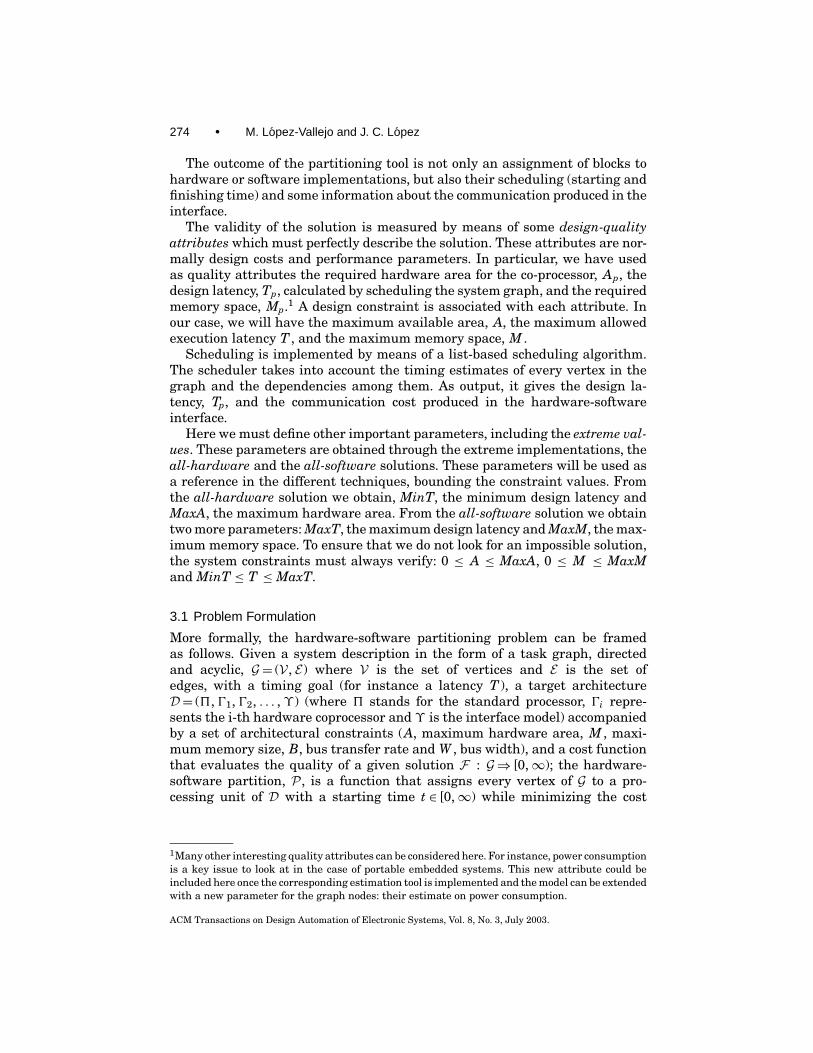
The global information flow of the partitioning procedure presented here isdepicted in Figure 1. The input to the partitioning process is an execution flowgraph that comes from the initial system specification, described using high-level specification languages. This is a directed and acyclic graph where verticesstand for basic computation units and edges represent data and control depen-dencies. Thus, vertices can be large pieces of information (tasks, processes, etc.)or small ones (instructions, operations), following respectively a coarse or finegranularity approach.

Every graph vertex is labeled with several attributes obtained after apply-ing estimation procedures [Carreras et al. 1996]. In detail, these pieces ofinformation for a node vi are: hardware area (hai), hardware execution time(hti), software memory size (ssi), software execution time (sti) and the aver-age number of times the task is executed (ni). Edges have also associated a



Fig. 1. Flow of information within the partitioning model.

communication value (tcomm(i, j )) obtained from three components: the transfertime (ttransf(i, j )), the synchronization time (tsynch(i, j )) and the average numberof times the communication takes place nij .

As is well known, system partitioning is clearly influenced by the target ar-chitecture onto which the hardware and the software will be mapped. Here thetarget architecture considered consists of one processor running the software,several dedicated co-processors (based on ASIC or FPGA) and shared memoryaccessed through a common bus. Interface modules are used to connect theprocessor and the ASIC to the bus. This is a model in which we have used justone hardware co-processor during our experiments for the sake of simplicity.Hardware and software processes can be executed concurrently in the standardprocessor and the application-specific co-processor.

In order to concentrate on the partitioning techniques, we have consideredthis architecture model that is very restrictive and simplifies the problem in thecontext of current architectures of embedded systems. Nevertheless, the modelwe have used can be extended to consider current system on chip architectures,as well as distributed embedded systems, supporting several programmableprocessors and complex communication structures.



The outcome of the partitioning tool is not only an assignment of blocks tohardware or software implementations, but also their scheduling (starting andfinishing time) and some information about the communication produced in theinterface.

The validity of the solution is measured by means of some design-qualityattributes which must perfectly describe the solution. These attributes are nor-mally design costs and performance parameters. In particular, we have usedas quality attributes the required hardware area for the co-processor, Ap, thedesign latency, Tp, calculated by scheduling the system graph, and the requiredmemory space, Mp.1 A design constraint is associated with each attribute. Inour case, we will have the maximum available area, A, the maximum allowedexecution latency T , and the maximum memory space, M .

Scheduling is implemented by means of a list-based scheduling algorithm.The scheduler takes into account the timing estimates of every vertex in thegraph and the dependencies among them. As output, it gives the design la-tency, Tp, and the communication cost produced in the hardware-softwareinterface.

Here we must define other important parameters, including the extreme val-ues. These parameters are obtained through the extreme implementations, theall-hardware and the all-software solutions. These parameters will be used asa reference in the different techniques, bounding the constraint values. Fromthe all-hardware solution we obtain, MinT, the minimum design latency andMaxA, the maximum hardware area. From the all-software solution we obtaintwo more parameters: MaxT, the maximum design latency and MaxM, the max-imum memory space. To ensure that we do not look for an impossible solution,the system constraints must always verify: 0 ≤ A ≤ MaxA, 0 ≤ M ≤ MaxMand MinT ≤ T ≤MaxT.

3.1 Problem Formulation

More formally, the hardware-software partitioning problem can be framedas follows. Given a system description in the form of a task graph, directedand acyclic, G= (V, E) where V is the set of vertices and E is the set ofedges, with a timing goal (for instance a latency T ), a target architectureD= (5, 01, 02, . . . ,ϒ) (where 5 stands for the standard processor, 0i repre-sents the i-th hardware coprocessor and ϒ is the interface model) accompaniedby a set of architectural constraints (A, maximum hardware area, M , maxi-mum memory size, B, bus transfer rate and W , bus width), and a cost functionthat evaluates the quality of a given solution F : G⇒ [0,∞); the hardware-software partition, P, is a function that assigns every vertex of G to a pro-cessing unit of D with a starting time t ∈ [0,∞) while minimizing the cost

1Many other interesting quality attributes can be considered here. For instance, power consumptionis a key issue to look at in the case of portable embedded systems. This new attribute could beincluded here once the corresponding estimation tool is implemented and the model can be extendedwith a new parameter for the graph nodes: their estimate on power consumption.



function F . Formally:

P : V⇒{5, 01, 02, . . . 0n} × [0,∞)/ ∀v∈V P(v)= (i, t) with

{i ∈ {5, 01, . . . 0n}t ∈ [0,∞)

F : G⇒ [0,∞) is minimized

It must also be verified that:

(1) ∀v1, v2 ∈V P(v1) 6=P(v2): condition of time-space exclusion.(2) ∀v1, v2 ∈V/v1< v2, (< expresses an order relation) i f P(v1)= (i, t1)

and P(v2)= ( j , t2)⇒ t1+ t(i, v1)< t2, condition of data dependenciesamong vertices, where t : D×V⇒ [0,∞) is a function that provides for everyvertex v∈V, its execution time in the processing unit i ∈ {5, 01, . . . 0n}.

(3) If vend ∈V/∀vj ∈V, vj 6= vend, vj < vend, P(vend)= (k, tfin)⇒ tfin+ t(k, vend)≤T ,condition of adjustment of time goal.

(4) Let 8hw be 8hw={vj ∈V, P(vj )= (k, t j )/k ∈ {01, . . . 0n}} it must be verifiedthat α(8hw) ≤ A, condition of adjustment of the area constraint, with α beingthe function that estimates the coprocessor hardware area with relation to8hw in a given point of the design space.

(5) Let 8sw be 8sw={vj ∈V, P(vj )= (k, t j )/k=5}; it must be verified thatµ(8sw) ≤ M , condition of adjustment of the memory size, with µ being thefunction that evaluates the memory space needed to run a software codewith relation to 8sw.

4. CLASSICAL PARTITIONING METHODS

The introduction of system-level issues within classical circuit partitioning al-gorithms is complex due to the different nature (hardware and software) ofthe processing elements. Consequently, the application of these partitioning al-gorithms requires strong modifications. In particular, the following algorithmshave been adapted to solve this problem: the simulated annealing stochastic al-gorithm, the Kernighan&Lin heuristic (K&L in the following) and hierarchicalclustering techniques.

4.1 Simulated Annealing

Simulated annealing [Kirpatrick et al. 1983] is a well-known optimization pro-cedure that emulates the physical annealing process. It can solve any combi-natorial optimization problem if the quality of the proposed solution can bemeasured by means of a cost function. This is the case of hardware-softwarepartitioning, which is why this method has been previously used to solve theproblem [Ernst et al. 1993; Eles et al. 1997]. Its major advantage is its gener-ality, while its main drawback is the long computation time required.

For simulated annealing to work, two main issues must be resolved: thecooling schedule and the cost function. We have used a dynamic cooling



schedule [Huang et al. 1986] for two main reasons:

—This schedule, based on the statistical definition of parameters, allows thealgorithm to work on a range of problems and does not require the tuning ofthe multiple algorithm parameters (cooling speed, equilibrium criteria, etc.)

—The algorithm convergence rate is much faster.

The formulation of the cost function is fundamental to obtaining good re-sults. The next section is devoted to the formulation of a general and efficientcost function [Lopez Vallejo et al. 2000]. Other approaches based on simulatedannealing deal with the cost-function straight-forwardly (just to minimize theexecution time [Ernst et al. 1993]) or pay little attention to the cooling sched-ule, consequently requiring the tuning the algorithm parameters for each exe-cution [Eles et al. 1997]. Recent work [Henkel and Ernst 2001] has improvedthese initial formulations and proposes the use of a dynamic cooling scheduleand defines a multi-objective function that trades diverse goals and constraints.This is performed in a way similar to the one proposed here [Lopez Vallejo et al.2000], but only for area and performance metrics, while our formulation candeal with many diverse attributes in a unified way.

4.1.1 Cost Function Formulation. The main goal of a cost function is tomeasure the quality of a given solution and to guide the algorithm to the bestsolution. As stated before, the important information related to system parti-tioning is:

—The global cost associated with the solution, measured by the quality at-tributes.

—The design constraints and goals.

Design constraints must define the design space and cost issues must helpmeasure the quality of the solution. The type of cost related to the qualityattributes must also be taken into account: fixed costs must be considered dif-ferently than variable costs. Our formulation incorporates all these points.

The proposed cost function includes several correction terms, FC(), for eachdesign goal affected by a specific constraint [Lopez Vallejo et al. 2000]. It canbe formulated as follows:

F(P)=∑

i

ki × Ci(P)Ci+∑

i

kciFC(Ci, Ci(P)) (1)

where Ci, the design constraint applied to the i-th quality attribute, Ci(P), ofa given solution P, has been used as a normalization parameter, and kci is theweight factor for the correction terms.

Three different techniques can be used to correct the objective function:

—Mean Square Error Minimization, which helps the algorithm find a solutiontuned to the constraints.

—Barrier Techniques, which forbid the exploration of solutions outside the al-lowed design space.



—Penalty Methods, which strongly punish the exploration of solutions thatwould produce medium or large constraints overhead, but allow the explo-ration of regions close to the boundaries defined by the constraints.

A typical way of tuning system constraints is minimizing the mean squareerror between quality attributes and their corresponding constraints. This kindof expression adjusts the attributes to the design goals and constraints. Thesefunctions can be applied to particular goals that should be completely fulfilledinstead of minimized. For instance, in the system partitioning problem, if thetarget architecture includes an FPGA-based coprocessor, it is a good policy tofully exploit all the resources the FPGA provides. This is due to the fact thatthe FPGA has a fixed cost, and its maximum exploitation generally resultsin performance improvement. Nevertheless, it would not be suitable for thosequality attributes that have variable cost, as they do in an ASIC area or timingmeasures.

The general expression for Mean Square Error based correction terms is:

FC(Ci, Ci(P))= (Ci(P)− Ci)2

C2i

(2)

This correction term, applied to the general expression shown in Equation (1),only contributes to the cost of the final solution when the attribute adoptsa value not tuned to the constraint. We should note here that this kind ofcorrection term equally penalizes any deviation from the design objective.

Barrier functions [Luenberger 1984] provide a clear boundary around thedesign space, in such a way that the cost associated with a solution outside ofthe design space will be infinity. This is performed by placing asymptotes inthe boundaries defined by the constraints. The analytical expression for theseterms is:

FC(Ci, Ci(P))= 1b[Ci, Ci(P)]

(3)

where b[Ci, Ci(P)] is the barrier function. An example of a barrier function canbe:

b[Ci, Ci(P)]=max {0, [Ci − Ci(P)]} (4)

This type of correction term can be used for hard design constraints, becauseit ensures that the constraint will never be violated. However, its applicationcontributes to the final cost of valid design solutions, requiring a careful ad-justment of the objective function weights and a modification of the final costinterpretation.

Finally, when the system constraints are not too hard, the use of penaltyfunctions [Luenberger 1984] may be more suitable. Penalty functions do notcontribute to the cost function when the solution is in the allowed search space.This kind of function is not so restrictive as the barrier functions, since solutionsaround the border of the allowed exploration region can be accepted if they arereally close. At this point, the weight factor kci is extremely important.



A general expression for penalty functions is the following:

FC(Ci, Ci(P))= r2[Ci, Ci(P)] (5)

where the function r[Ci, Ci(P)] corresponds to:

r(Ci, Ci(P))=max{

0,[Ci(P)− Ci]

Ci

}(6)

4.2 The Kernighan&Lin Heuristic

The original circuit partitioning heuristic was proposed by Kernighan and Linin 1970 [Kernighan and Lin 1970]. It is based on iterative improvement, butallows the partitioning process to escape from some local minimum. The algo-rithm starts with an initial random partition and swaps nodes between bothsides of the partition. All the nodes are interchanged following the order pro-vided by the best gain (maximum decrease or minimum increment of nets in thecut set). The best solution found during the swap process is recorded and usedas the new initial partition in the following iteration. The algorithm finisheswhen no further improvement is achieved.

Fiduccia and Mattheyses [1982] improved the algorithm performance bymeans of a sophisticated data structure, the bucket array. This structure guar-antees linear access time when determining the best movement, taking advan-tage of the bounded integer gain produced when a node crosses the interface.

The work of Prof. Vahid [1997] in this kind of adaptation is very interesting,but his extension of the algorithm cannot be applied to any other hardware-software partitioning environment, due to the limitations of the model used inthe formulation of the system partitioning. This model is defined over an accessgraph (the SLIF graph [Vahid and Gajski 1995b]), which eases the computationof magnitudes related to the current design (every design quality parameter iscomputed by adding the different values of the attributes associated with thenodes and edges), but introduces serious limitations:

(1) The design cannot be scheduled, which makes estimating time very rough.(2) Since any estimation performed in the SLIF graph will be done by adding

the node attributes, the trivial solution with everything implemented ashardware will appear in all the optimization procedures. This represen-tation ignores the parallelism inherent to a multiprocessor architecture,whose consideration can provide better results when using a standard pro-cessor and a dedicated coprocessor.

The extension of the Kernighan and Lin method to solve the hardware-software partitioning problem must take into account several features:

—The main objective of a hardware-software partitioning tool is much morecomplex than the simple net cut. Different design aspects must be considered:essentially performance goals and design costs.

—The incremental evaluation of the cost function is not possible because com-plex measurements must be taken at every step of the algorithm.



The system model presented previously compensates for all these disadvan-tages allowing the extension of the algorithm to deal with the complex infor-mation related to system level design. First, the cost function introduced inSection 4.1.1 can properly handle the system design. Second, a different datastructure can improve the algorithm convergence rate. The proposed cost func-tion perfectly characterizes the current design quality, but it is done by meansof real numbers. Thus, the integer gain-based bucket-array structure cannot beused for the system partitioning problem.

We have defined a data structure based on maps instead of arrays. A map isa sorted associative container that associates objects of type Key with objectsof a given type. It is also a unique associative container, meaning that no twoelements ever have the same key. We have used as a key the cost incrementassociated with a given movement, and as data the node that should be moved.Since more than one node could produce the same cost variation we have useda multi-map structure. A multi-map is a sorted associative container that as-sociates objects of type Key with objects of a given type. It is also a multipleassociative container, meaning that there is no limit on the number of elementswith the same key.

The proposed data structure is bounded by the number of nodes containedby the system graph. The standard template library implementation of thesestructures [Stroustrup 1997] guarantees that given a key the associated datais found through a search with logarithmic complexity.

4.3 Hierarchical Clustering

Another classical heuristic used for circuit and architectural partitioning ishierarchical clustering. This is a constructive method that groups pairs of par-titioning objects based on a proximity value between the objects. The algorithmis fully characterized after defining the following issues:

—The closeness function that provides the proximity values.—The cut level in the cluster tree that is built upon the closeness values.

Both issues will be modified to distribute a given functionality among het-erogeneous implementation units [Lopez Vallejo and Lopez 2001]. This is againdue to the different nature of the target processing units. It is obvious that acloseness metric used to group objects that will run in a standard processorcannot be suitable for those objects implemented with dedicated hardware.

The proposed closeness function takes into account the system model infor-mation. In particular, it uses the estimates associated with the vertices andedges of the system graph G(V, E) in the following way: the function groupsthose partitioning objects with a clear tendency to be implemented as hard-ware. Actually, every algorithm iteration selects the two objects with the besttime improvement when implemented as hardware (the highest latency de-crease). Objects not grouped along the process will be assigned to the softwareprocessing unit. The cut level is dynamically computed whenever a cluster isgrown taking into account the system constraints. It can be said that this is asoftware-oriented approach, since all objects are supposed to originally reside in



Fig. 2. Clustering process: evolution of the area and latency quality attributes versus their re-spective constraints.

software and during the process they are extracted to the hardware processingunit.

With this procedure, the whole cluster tree does not need to be built. Everytime a cluster is grown, the area and latency constraints (A and T ) are checked.The cluster tree construction stops whenever:

(1) The time constraint is met (Tp<T ) and the hardware area value is belowits corresponding constraint (Ap< A).

(2) The hardware area constraint is exceeded (Ap> A) while the latency con-straint is not yet met (Tp>T ).

In the first case, area and latency constraints are met and the algorithm isalmost finished (only the memory constraint must be checked). In the secondcase, the area constraint is met without fulfilling the timing objectives, andtherefore, a refinement phase is necessary. This can be accomplished by somelocal search procedure working with objects with smaller grain (thus, the lastgroups must be separated).

Our approach is based on the idea that to find a solution there must beseveral points in the design space satisfying their respective constraints, as canbe seen in Figure 2. This plot shows the evolution of the area and latency qualityattributes normalized with respect to the design constraints while building thewhole cluster tree in a clustering process. Axis X shows the number of iterationsin the clustering process (number of clusters grown). As the number of clustersadded to the tree increases, the hardware area becomes larger and the designlatency should decrease. When time and area constraints are satisfied, thememory constraint should be checked, although playing a secondary role. Ifthe memory constraint is met, the algorithm finishes. Otherwise the clustergrowth continues while other (primary) constraints are still under their limits.Figure 3 illustrates the algorithm control flow described above.

Now we will take a look to the closeness function formulation. As is wellknown, the exchange of information among the different processing units ofthe architecture penalizes the design latency. Closeness metrics attempt to



Fig. 3. Control scheme of the clustering process.

reduce this problem. In addition, since the algorithm follows a “hardware ex-traction” approach the time improvement obtained when extracting an objectto hardware should also be considered. The expression we have formulated asa closeness function that takes into account both effects is the following:

Ci, j =qT ×(

ni1ti

sti+ nj

1t j

st j

)+ qC × tcom(vi, vj )

tr com(vi)+ tr com(vj )(7)

where1ti = sti−hti represents the time improvement obtained when the objecti is moved from software to hardware. The function tcomm(vi, vj ) computes thecommunication between nodes vi and vj in the interface following a generalmodel of the architecture [Lopez Vallejo 1999]. The weight factors qT and qChelp the designer emphasize which factor he/she wants to optimize.

As can be seen, every function term has been normalized against its soft-ware time, in such a way that the resulting closeness value is greater for thoseobjects with bigger difference between hardware and software execution times.The communication term has been normalized with respect to the addition ofcommunication values of the cluster object with other objects of the systemgraph, its expression being the following:

tr com(vi)=∑vk∈V

tcom(vi, vk)/∃ (vi, vk)∈ E (8)

We have used this kind of normalization to highlight the fact that the com-munication between two design modules must be considered only when there



are many transfers between these modules alone. This term will be thereforeless important when communication with the rest of the design modules isconsiderable.

When checking the plausibility of this closeness function several deficien-cies in the behavior of the algorithm were observed. In some cases the algo-rithm grouped objects with very high communication values and a good timeimprovement, but with a considerable size. This halted the algorithm early be-cause of the hardware area constraint. For this reason the closeness functionwas modified to cluster objects that had the previous time and communicationconsiderations but which required little hardware area. The resulting functionexpression is:

Ci, j =qT ×(

ni1ti

sti+ nj

1t j

st j


tr com(vi)+ tr com(vj )+ qA

no × MaxA|V|

hai + ha j(9)

where a hardware area term, controlled by its corresponding weight factor qA,has been introduced. This term has a clear meaning: its value is greater whenthe area of the resulting cluster is smaller than the average system area. Thisaverage area is computed by dividing the area of the all-hardware solution,MaxA, by the total number of vertices of the system graph G(V, E) given bythe cardinal of V, |V|. The parameter no is the number of nodes integratingthe cluster, no= |i| + | j |. As will be described, each clustering object (single orcomposed) will be characterized with the same attributes as the nodes of thesystem model, hai, hti, and so forth. This formulation allows us to handle objectswith different size or various components in a uniform way.

In the same way we can introduce a term for considering the memory space.In this case, since we are extracting modules to hardware, the memory termmust try to group objects with large-sized memory. This value is also computedusing the parameter MaxM provided by the all-software solution. The finalexpression for the closeness function for two objects, i, j , is:

Ci, j = qT ×(

ni1ti

sti+ nj

1t j

st j


tr com(vi)+ tr com(vj )

+qAno × MaxA

|V|hai + ha j

+ qMssi + ss j

no × MaxM|V|

(10)

It is important to remark that the resulting clusters must exhibit the samecharacteristics as the basic objects, in such a way that no cumulative error isintroduced. This characterization allows us to use the same closeness functionthroughout the algorithm’s execution. Consequently, we define the followingapproximation to characterize a cluster k= i ∪ j :

—The resulting hardware area is computed by adding up of the hardware areaof the nodes that integrate the cluster.

hak =∑vn∈pi

han +∑

vm∈pj

ham (11)



This estimation is quite rough, because it does not take into account resourcesharing. Nevertheless the approach is completely valid, and we leave forfuture study the improvement of the area-estimation procedures.

—The cluster memory space is computed as the sum of the memory sizes of itscomposing vertices.

ssk =∑vn∈pi

ssn +∑

vm∈pj

ssm (12)

—The cluster execution time in a standard processor is the sum of the softwareexecution times, of its composing nodes, due to the code serialization.2

stk =∑vn∈pi

stn +∑

vm∈pj

stm (13)

—The resulting hardware execution time can be computed in two differentways:(1) If there are no data dependencies among the cluster vertices, concurrency

is possible, and the hardware execution time is given by:

htk =max{htn with vn ∈ pi ∪ pj } (14)

(2) If there are data dependencies the cluster vertices must be scheduled.Since at every algorithm iteration a system scheduling is performed, wehave the starting and finishing times of all the vertices, so the clusterexecution time is therefore:

htk =max{tend(vn)} −min{tend(vn)} − tidle with vn ∈ pi ∪ pj (15)

where tidle is the time the hardware co-processor is idle betweenmin{tend(vn)} and max{tend(vn)}. This kind of timing evaluation has twoclear advantages. First, there is no cumulative error, because htk is recal-culated at every step of the algorithm. Second, the computational com-plexity is not greater, since we take advantage of the scheduling per-formed to evaluate design constraints.

Regarding the cluster edges, we will only consider the edges coming in andout of the cluster, canceling the edges within the cluster vertices. The exter-nal edges keep their original attributes, because the cluster will be consideredexactly as a new system vertex.

Even though hierarchical clustering has been used for hardware-softwarepartitioning, our approach is very different from these previous implementa-tions. It is mainly due to the formulation of the closeness metric and the mod-ification of the control scheme of the algorithm. In Vahid and Gajski [1995a]different and interesting closeness metrics are defined, but their application isnot straightforward and their use is not clearly described. We believe that the

2The cluster execution time in the software processor only considers the time spent in this particu-lar execution unit, which is subject to improvement if implemented as standard hardware. It mayhappen that due to communication delays the finishing time of the cluster is longer than the valueestimated here. This is not important in our model, because the communication cost is already con-sidered when the cluster is grown and scheduling is performed. stk only characterizes an intrinsicparameter of the cluster.



closeness metrics must be different for the hardware and the software parti-tions. Thus, the clustering procedure needs to be modified and specific metricsfor the different implementation units must be defined. Additionally, we havedefined a problem model which helped us introducing important modificationsto the original algorithm. In Barros et al. [1993], other closeness metrics areintroduced, mainly based on the specification language UNITY. Nevertheless,cost issues, as we propose in this work, are not considered.

5. KNOWLEDGE-BASED PARTITIONING

Knowledge-based techniques can be used to solve many optimization problemsby working at a higher abstraction level [Newell 1982], because the knowledgeacquired by the designers can be modeled and conserved, even if the technol-ogy used to develop the partitioning tool becomes obsolete. We have developed afuzzy logic based expert system, SHAPES (Software-Hardware Partitioning Ex-pert System [Lopez Vallejo et al. 1998]), following the CommonKADS method-ology [Breuker and Van de Velde 1993]. This tool takes advantage of two impor-tant contributions of artificial intelligence: the use of an expert’s knowledge inthe decision making process and the possibility of dealing with imprecise andusually uncertain values by the definition of fuzzy magnitudes.

The main benefits of a knowledge-based approach are:

—The designer’s knowledge is acquired for automatic handling, while the re-sults obtained by traditional procedures must be reviewed by a designer.

—The whole process can be traced.—Knowledge of the system can be increased by applying it to different cases.

There is also a solid rationale to use fuzzy logic:

—Since the designer’s knowledge is imprecise in nature, fuzzy logic can be usedto include the subjectivity implicit in the designer’s reasoning.

—Most data are estimates, which can be easily modeled with fuzzy linguisticvariables. For instance, the area estimate of a block is modeled as a linguisticvariable with the terms {small, medium or large} (Figure 4). Since this valuedepends on the particular system under evaluation, the linguistic variablehas been dynamically defined according to a granularity measure, σ :

σ = 100i

i being the number of vertices to consider.—Some of the parameters defined along the process exhibit intrinsic looseness.

For example, Figure 5 shows the implementation value of a task, which re-flects the tendency of the task to be implemented as hardware or software. Inthis case, we can talk for instance about a quite hardware or a very softwareblock.

The expert system construction has adopted a knowledge-modeling ap-proach, following the knowledge level and knowledge separation principles.The expertise model is, then, the center of the knowledge-based systemdevelopment.



Fig. 4. Linguistic variable Area.

Fig. 5. Linguistic variable Implementation.

5.1 Expertise Model of Hardware-Software Partitioning

Three main issues must be addressed when an expertise model is constructed:an ontology of the domain knowledge, the task knowledge and the inferencestructure. The domain ontology provides the most important concepts and re-lations of a given domain. The task knowledge specifies how a task is relatedto the task objective. Actually it describes the way a goal can be achieved bymeans of some control mechanisms. The inference structure is a compound ofpredefined inference types (how the domain concepts can be used to make in-ferences, represented as ellipses) and domain roles (rectangles), as can be seenin Figure 6. For the purpose of this paper, we will only describe the inferencestructure. We refer readers interested in deeper explanations of the expertisemodel to [Lopez Vallejo et al. 1999].

The inference structure shown in Figure 6 presents a general view of theproblem solving method (PSM) chosen to implement system partitioning andthe knowledge used by the inferences. This generic inference structure will beadapted to our problem.



Fig. 6. Inference structure for hardware-software partitioning.

According to the CommonKADS library [Breuker and Van de Velde 1993], thepartitioning task has been classified as a configuration task with antagonisticconstraints. The Propose and Revise (P&R) problem solving method, whoseinference structure is shown in Figure 6, has been followed. An initial heuristicclassification is carried out before the standard P&R for providing additionalinformation to the propose task.

Following the inference structure, four inferences can be distinguished:match (Section 5.2.1), assign (Section 5.2.2), evaluate (Section 5.2.3), and select(Section 5.2.4). This inference structure has guided the knowledge-acquisitionprocess.

5.2 Partitioning Design Model

The design of the system has followed a structure-preserving approach, defin-ing a module for each knowledge source of the defined inference structure(Figure 6).



5.2.1 Match (Heuristic Classification). The first step in SHAPES is to pro-vide additional information for the P&R method. It is performed by means ofa heuristic classification module. In this module, the observables are the es-timates attached to every vertex properly converted into fuzzy variables. It isimportant to remark that all the fuzzy sets are dynamically defined, becausetheir values are relative to the specific example under study (see Figure 4).

The heuristic rules stored in the knowledge base match the input vari-ables and the output variable, called implementation. The terms this vari-able can adopt are {Hardware, Quite-Hardware, Unknown, Quite-Software, andSoftware}. This variable gives an idea of the intrinsic tendency of a processto be implemented in special purpose hardware or as software running on astandard processor. An example of the rules of this module follows:

if hw-area is small and time-improvement is highand number-executions are not few

then implementation is very hardware

5.2.2 Assign. The assign inference provides the first solution proposal byallocating part of the processes to hardware and the rest to software. In thismodule the observables are the system blocks with their related implementa-tion values and the system constraints (maximum hardware area, A, maximumexecution time, T , and maximum memory space, M ). The module produces asoutput a threshold that determines the hardware-software boundary.

The threshold value is obtained after estimating the “hardness” of the spec-ification requirements: how critical (or not) the constraints are, regarding theextreme values of the system performance (all hardware and all software solu-tions). Upon this parameter, a system configuration is composed.

Every process implementation variable is defuzzified to obtain its crisp valueand consequently an initial partition. It is necessary to provide standard outputresults since they will be used in standard tools like the scheduler. This crispclassification output is the set of input blocks ordered by their implementationdegree: value 0 stands for hardware and 1 for software. For instance, Figure 7shows the results for an example with 23 processes after performing the as-signment operation, defuzzifying the threshold and implementation values.

5.2.3 Evaluate. The evaluate module computes the different parametersthat characterize the design obtained after assignment. These parameters willgive an idea of the quality and acceptability of the proposal. This is the onlymodule not based on knowledge. Here four parameters have been considered:

(1) The estimation of the area needed to implement the hardware part, Ap.(2) The estimation of the memory space required by the software code and data,

Mp.(3) The scheduling of the assigned process graph, which gives the final execu-

tion time or latency, Tp.(4) The communication costs in the hardware-software interface, which con-

sider two different aspects: the total number of transfers that take placein the hardware-software interface, and the communication penalty, which



Fig. 7. Classification and assignment results for the case study.

computes the global delay introduced in the system execution time due tospecific communication waiting.

Once these parameters have been calculated, the select inference will checkthe plausibility of the proposed partition. With this purpose, additional infor-mation is then generated to determine the state of the constraints. Specifically,the following variables are defined:

—The area, memory and time overhead :1A= A−Ap,1M =M−Mp,1T =T−Tp.

—The communication penalty.—The processor and ASIC throughputs, defined as:

τproc=∑

i ∈ SWsti

Tpτasic=

∑i∈HW

hti

Tp

5.2.4 Select. The select inference executes the most complex inference inSHAPES. This is a composite inference where two other inferences have beendefined. Its purpose is to revise the proposed solution and to search for anotherproposal. Consequently, the select strategy has been divided into two stages:

(1) Diagnosis, which studies how closely the solution comes to the optimumand how many corrections are needed.

(2) Operation, which performs the selection of a new proposal based on theprevious information and a knowledge base of previous experiences.



Fig. 8. Control flow within the composed select inference.

Figure 8 shows the dependencies among these sub-tasks, specifying thecontrol knowledge within this inference. The diagnosis module performs asimple analysis, identifying the state of the design regarding initial goalsand constraints and carrying out the revision procedure of the P&R PSM. Inthis simple diagnosis inference the following observable categories have beenconsidered:

—The violation or satisfaction of the hardware area and global time constraints(upon their respective gaps).

—The balance of the proposal, regarding the processor and ASIC throughputs(τproc/τasic ≈ 1).

—Which vertices are related to the communication penalty.

Taking these symptoms into account, two kinds of revisions can be performed.First, if the system constraints are not met, the method must refine the solutionto find a feasible one. Second, if constraints are met, but the attribute valuesare very large, the solution can be refined to reduce costs.



Table II. Set of Examples Provided by Dr. SrinivasanCharacterized by the Number of Vertices and Parameters of

the Extreme Solutions

Example Vertices MaxA MinT MaxT MaxMlu 9 69315 74 454 19595fft 15 106355 145 842 33619dct 9 21952 2231 7312 329692dct16 36 34944 6712 20680 1143982laplace 9 73009 79 386 17811mean 9 132626 99 607 27244reg 8 3379 1890 6714 303288

The operation module performs the proposal of the new partition, if needed.There are two non-exclusive alternative strategies to choose:

—To migrate processes from hardware to software or vice versa according tothe global constraints. This is carried out by tuning the threshold.

—To improve the partition while attempting to minimize the communicationon the hardware-software boundary. This is performed by communication-based reordering, that modifies the classification results according to thecommunication penalty produced on the interface.

6. ANALYSIS OF RESULTS

All the techniques have been applied to a set of examples provided by Dr. Srini-vasan [Srinivasan et al. 1998], whose characterization appears in Table II:the size of the system graph and the values of the extreme implementations,which bound the design space. The examples are described as directed andacyclic graphs of coarse-grain tasks. We have applied the four partitioning tech-niques to every example using different constraints (always within the boundsprovided by the extreme solutions). The examples have been subjected to in-tensive experiments, the results of which are summarized in Table III. Theseresults will be analyzed from both qualitative and quantitative perspectives.3

The qualitative aspects will be mainly represented by the resulting cost of thesolutions obtained from each method, under different constraints. The quanti-tative issues will be shown by means of the computation time resulting fromeach technique.

For simulated annealing and K&L the penalty-based cost function(Section 4.1.1) has been used. This formulation has been chosen after check-ing the behavior of all the proposed cost functions, and proving that this wasthe best for a general system partitioning problem. Therefore, the quality at-tributes are always optimized within their respective constraints. The resulting

3These results cannot be compared to the ones presented in [Srinivasan et al. 1998] because in thiswork the partitioning phase integrates hardware design exploration, while we have chosen a givenhardware implementation for every task in our experiments.



Table III. Results Obtained with the Examples Provided by the University of Cincinnati

Constraints Simulated Annealing Kernighan&LinEx. A T M Ap Tp Mp Cs. Ap Tp M p Cs.LU 15000 400 17000 9110 404 14856 0.588 38501 176 6099 0.806

30000 200 16000 27311 206 9594 1.177 25604 193 9757 0.65650000 150 12000 47611 126 1360 0.624 47611 126 1360 0.849

FFT 30000 400 25000 32464 424 19902 2.674 30530 470 22020 5.98660000 250 25000 58092 255 14747 0.824 61619 256 10928 1.03580000 200 15000 78242 199 2860 0.611 73337 195 8180 0.772

DCT 16000 4000 100000 13720 2822 73212 0.796 13720 2825 60076 0.52913000 5500 200000 5488 5372 164125 0.652 8232 4254 134701 0.48920000 3000 120000 13720 2822 73212 0.849 8232 4762 269616 0.538

DCT16 10000 20000 800000 8736 15510 796866 0.594 8736 14450 761912 0.72420000 15000 800000 — — — — 17472 9280 364505 0.56030000 16000 750000 — — — — 17472 9280 415821 0.404

Laplace 20000 250 16000 16059 251 11232 0.615 20099 260 14894 1.55030000 200 15000 29401 179 7280 0.611 31668 229 10023 1.04050000 200 12000 38358 137 4200 0.471 14588 320 13345 0.488

Mean 60000 300 20000 55679 294 13938 0.792 55679 294 13938 0.94280000 500 10000 76252 313 10164 0.616 100354 239 5740 0.738

120000 200 10000 116517 127 3124 0.513 116517 127 3124 0.513Reg 3000 2500 40000 2407 2590 13180 0.779 2113 2380 29029 0.682

2500 3000 35000 2407 2590 13180 0.585 2407 2590 13180 0.5852000 4000 50000 2208 2313 26918 2.181 1435 2030 44043 0.455

Constraints Clustering Expert SystemEx. A T M Ap Tp Mp Cs. Ap Tp M p Cs.LU 15000 400 17000 9619 356 16463 0.556 14377 333 13112 0.63

30000 200 16000 25604 193 9757 0.606 30362 170 6406 0.6050000 150 12000 34714 143 5018 0.536 34714 143 5018 0.53

FFT 30000 400 25000 28764 557 18633 23.89 27957 456 23576 1.2760000 250 25000 59054 265 7880 1.573 60723 244 12797 0.8880000 200 15000 78192 172 3526 0.575 74605 207 8054 0.68

DCT 16000 4000 100000 10976 3675 75013 0.556 13720 3390 38136 0.5513000 5500 200000 5488 5372 164125 0.502 10976 3408 85747 0.5020000 3000 120000 13720 2825 48779 0.529 13720 2825 48779 0.53

DCT16 10000 20000 800000 4368 16240 776552 0.472 7644 14500 535014 0.5320000 15000 800000 7644 14500 628607 0.483 17472 9287 258506 0.5230000 16000 750000 5460 15660 721591 0.444 17472 9287 220625 0.49

Laplace 20000 250 16000 17132 274 9013 2.024 16059 251 11232 0.7230000 200 15000 23921 213 7631 1.243 29401 179 7280 0.6150000 200 12000 37263 141 3679 0.536 43989 115 2814 0.47

Mean 60000 300 20000 43865 386 15438 13.01 55241 292 21751 0.7480000 500 10000 76137 260 9698 0.538 72316 259 9898 0.59

120000 200 10000 103603 176 4676 0.570 105160 135 5022 0.50Reg 3000 2500 40000 2407 2590 13180 0.779 2407 2590 13180 0.78

2500 3000 35000 2407 2590 13180 0.585 2167 2863 11285 0.592000 4000 50000 1435 2030 44043 0.455 1873 3354 47005 0.56



Fig. 9. Cost values obtained when running the Cincinnati University examples.

cost function is:

F(P) = kA × Ap

A+ kT × Tp

T+ kM × Mp

M+ kcAFC(A, Ap)+ kcTFC(T, TP )+ kcMFC(M , Mp) (16)

The following weight factors have been applied in all tests: ka= 0.3, kt = 0.4,km= 0.3 and kci = 150. These factors allow the designer to put emphasis on thedesired design attribute. In these examples, the time goal is slightly empha-sized. If these factors are appropriately chosen, they can also help to interpretthe results. For instance, when

∑i ki = 1 (as in our case) thenF(P)= 1 is a figure

of merit, since (1) constraint overheads will produce cost values much greaterthan 1 (due to the penalty weight factor kci = 150), (2) attribute values tunedto the constraints will produce costs close to the unity, and, (3) if the solutioncould be optimized (penalty terms are used) the cost value will be lower than 1.

For hierarchical clustering and the expert system, once we have the resultsprovided by these methods (driven by the closeness function or the knowledgebases respectively), we have used the same cost function to characterize thequality of the solutions found and to compare results more easily.

6.1 Solution Quality

In Figure 9 we have represented the cost of the solutions computed by all themethods under evaluation. Each example has been checked with four sets ofconstraints (defined in Table III) represented in the figure as four points in theaxis X. These four sets of constraints have been ordered from harder to softer.



Fig. 10. CPU times (in seconds) for the different partitioning techniques with the CincinnatiUniversity examples.

A first analysis of the results shows that for hard constraints the heuristicalgorithms (clustering and K&L) cannot find a valid solution. Even worse, thesealgorithms provide solutions quite far from the valid region. On the other hand,simulated annealing and the expert system can find solutions for these hardconstraints or at least give solutions not far from the allowed exploration region.We can conclude that these two methods provide the best results concerningsolution quality. If the constraints are not too hard, all the methods can providea workable solution.

6.2 Computation Time

The computation time of the different methods under study has been repre-sented in the histogram of Figure 10. Axis Y represents the CPU time spentby the example resolution (simulated annealing time appears divided by 15 forthe sake of clarity).

After executing all the examples and examining Figure 10, it is clear that thefastest technique is the clustering algorithm. The reason why this procedureis faster is that it performs the system scheduling very few times (only whena cluster is grown). The other classical algorithms must schedule the design ateach trial. Consequently, simulation annealing requires the longest computa-tion time, since the number of explored points of the design space is much morelarger than in the other methods.

The expert system expends more time than the K&L and the clustering, butalways within reasonable values and much lower than the simulated annealing.



Fig. 11. CPU times (in seconds) for the different partitioning methods vs. the example size.

This longer execution time is partly due to the use of an interpreted inferenceengine [Lyndon B. Johnson Space Center 1993]. A future study could seek toobtain a faster version of the expert system by compiling its knowledge bases.This has not been done because of the continuous refinement of the system rules.

Finally, to test the behavior of the partitioning techniques when workingwith bigger examples we have generated several system graphs with a greaternumber of vertices (from 50 to 500 nodes). Figure 11 represents the executiontimes obtained after running these examples, ordered by size. These experi-ments confirmed the results obtained previously.

6.3 Lessons Learned

The experiments we have performed with the various partitioning implementa-tions have shown that this problem can be solved by very different techniques.We can conclude, as a first lesson, that it is very important to build the differ-ent implementations over a complete and robust model, which holds all vitalinformation and allows us to deal with different problems.

Simulated annealing has provided the best results from a qualitative pointof view, but its computations take a very long time. This occurs even afterapplying a dynamic cooling schedule, which facilitates the algorithm conver-gence. On the other hand, the experiments performed with K&L and clusteringhave shown that these algorithms produce a good trade-off between quality ofresults and computation time, even though they show an irregular behavior.The K&L algorithm depends too much on the initial solution (here calculatedrandomly). This problem can be easily solved by starting from a better solution



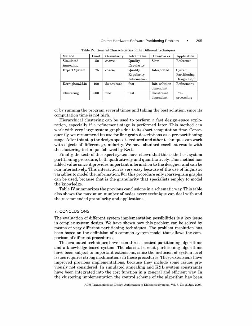
Table IV. General Characteristics of the Different Techniques

Method Limit Granularity Advantages Drawbacks ApplicationSimulated 50 coarse Quality Slow ReferenceAnnealing RegularityExpert System 75 coarse Quality Interpreted System

Regularity PartitioningInformation Design help

Kernighan&Lin 100 do not care fast Init. solution Refinementdependent

Clustering 500 fine fast Constraint Pre-dependent processing

or by running the program several times and taking the best solution, since itscomputation time is not high.

Hierarchical clustering can be used to perform a fast design-space explo-ration, especially if a refinement stage is performed later. This method canwork with very large system graphs due to its short computation time. Conse-quently, we recommend its use for fine grain descriptions as a pre-partitioningstage. After this step the design space is reduced and other techniques can workwith objects of different granularity. We have obtained excellent results withthe clustering technique followed by K&L.

Finally, the tests of the expert system have shown that this is the best systempartitioning procedure, both qualitatively and quantitatively. This method hasadded value since it provides important information to the designer and can berun interactively. This interaction is very easy because of the use of linguisticvariables to model the information. For this procedure only coarse-grain graphscan be used, because that is the granularity that specialists employ to modelthe knowledge.

Table IV summarizes the previous conclusions in a schematic way. This tablealso shows the maximum number of nodes every technique can deal with andthe recommended granularity and applications.

7. CONCLUSIONS

The evaluation of different system implementation possibilities is a key issuein complex system design. We have shown how this problem can be solved bymeans of very different partitioning techniques. The problem resolution hasbeen based on the definition of a common system model that allows the com-parison of different procedures.

The evaluated techniques have been three classical partitioning algorithmsand a knowledge based system. The classical circuit partitioning algorithmshave been subject to important extensions, since the inclusion of system levelissues requires strong modifications in these procedures. These extensions haveimproved previous implementations, because they include some issues pre-viously not considered. In simulated annealing and K&L system constraintshave been integrated into the cost function in a general and efficient way. Inthe clustering implementation the control scheme of the algorithm has been



modified and new closeness metrics have been defined. Artificial intelligencetechniques are very promising to model and work with system level issues asa consequence of the quality of the results and the extra information providedto the user.

The use of these techniques has proven to be effective, as some experimentshave shown. Table IV summarizes the conclusions we have drawn after execut-ing and comparing the different system partitioning methods.

A future study could extend the system model to encompass other qualityattributes, like power consumption or the degree of parallelism. Also, the finalrefinement of the knowledge bases of the expert system and their compilationare currently under study.

ACKNOWLEDGMENTS

We would like to thank Carlos Angel Iglesias for his insights into artificialintelligence; Antonio Garcia Quintas for his contribution with the developmentof the scheduler; and Jesus Grajal for his help in the formulation of the costfunction.

REFERENCES

BARROS, E., ROSENSTIEL, W., AND XIONG, X. 1993. HW/SW Partitioning with UNITY. In Handoutsof the 2nd International Workshop on HW-SW Codesign.

BREUKER, J. A. AND VAN DE VELDE, W., Eds. 1993. The CommonKADS Library. Netherlands EnergyResearch Foundation ECN, Swedish Institute of Computer Science, Siemens, Univ. of Amsterdamand Free University of Brussels. Tech. rep., ESPRIT Project P5248.

CARRERAS, C., LOPEZ, J. C., LOPEZ-VALLEJO, M. L., DELGADO-KLOOS, C., MARTıNEZ, N., AND SANCHEZ, L.1996. A Co-Design Methodology Based on Formal Specification and High-Level Estimation. InProceedings of the Workshop on HW/SW Co-Design.

DICK, R. AND JHA, N. 1998. Mogac: a multiobjective genetic algorithm for hardware-softwarecosynthesis of distributed embedded systems. IEEE Trans. CAD Int. Circ. Syst. 17, 10 (Octo-ber), 920–935.

ELES, P., PENG, Z., KUCHCINSKI, K., AND DOBOLI, A. 1997. System Level Hardware/Software Par-titioning based on Simulated Annealing and Tabu Search. Design Automation for EmbeddedSystems 2, 1 (January), 5–32.

ERNST, R., HENKEL, J., AND BENNER, T. 1993. Hardware-Software Cosynthesis for Microcontrollers.IEEE Des. Test Comput. 64–75.

FIDUCCIA, C. AND MATTHEYSES, R. 1982. A Linear-time Heuristic for Improving Network Partitions.In Proceedings of the Design Automation Conference. IEEE.

GUPTA, R. K. AND MICHELI, G. D. 1993. HW-SW Cosynthesis for Digital Systems. IEEE Des. TestComput. 29–41.

HENKEL, J. AND ERNST, R. 2001. An approach to automated hardware/software partitioning usinga flexible granularity that is driven by high-level estimation techniques. Trans. VLSI Syst. 273–289.

HUANG, M. D., ROMEO, F., AND SANGIOVANI-VINCENTELLI, A. 1986. An Efficient General Cooling Sched-ule for Simulated Annealing. In Proceedings of the Design Automation Conference. 381–384.

KALAVADE, A. AND LEE, E. A. 1997. The Extended Partitioning Problem: Hardware/Software Map-ping, Scheduling and Implementation-bin Selection. J. Design Automat. Embedded Syst. 2, 2(March), 125–164.

KERNIGHAN, B. W. AND LIN, S. 1970. An Efficient Heuristic Procedure for Partitioning Graphs. TheBell System Technical Journal. 291–307.

KIRPATRICK, S., GELATT, C., AND VECCHI, M. 1983. Optimization by simulated annealing. Sci-ence 220, 4598, 671–680.



LOPEZ VALLEJO, M., GRAJAL, J., AND LOPEZ, J. C. 2000. Constraint-driven System Partitioning. InProceedings of DATE’00. 411–416.

LOPEZ VALLEJO, M., IGLESIAS, C., AND LOPEZ, J. C. 1998. A Knowledge based System for Hardware-Software Partitioning. In Proceedings of DATE’98. 914–915.

LOPEZ VALLEJO, M. AND LOPEZ, J. C. 2001. Multi-way Clustering Techniques for System LevelPartitioning. In Proceedings of the 14th IEEE ASIC/SOC Conference. 242–247.

LOPEZ VALLEJO, M., LOPEZ, J. C., AND IGLESIAS, C. 1999. Hardware-Software Partitioning at theKnowledge Level. J. Applied Intell. 173–184.

LOPEZ VALLEJO, M. L. 1999. Hardware-software partitioning methods for the design of heteroge-neous systems. Ph.D. thesis, Universidad Politecnica de Madrid.

LUENBERGER, D. G. 1984. Linnear and non-Linear Programming. Addison-Wesley.LYNDON B. JOHNSON SPACE CENTER. 1993. Clips’s Reference Manual. Volume II, Advanced Program-

ming Guide. CLIPS Version 6.0. Lyndon B. Johnson Space Center, Software Tecnology Branch.MADSEN, J., GRODE, J., AND KNUDSEN, P. 1997. Hardware/software partitioning using the lycos sys-

tem. Hardware/Software Codesign: Principles and Practices (chapter 9). Kluwer Academic Pub-lishers.

MICHELI, G. D. 1994. Guest editor’s introduction: Hardware-Software Codesign. IEEE Micro. 8–9.NEWELL, A. 1982. The knowledge level. Artificial Intelligence. 87–127.NIEMANN, R. AND MARWEDEL, P. 1996. Hardware/software partitioning using integer programming.

In Proceedings of the European Design & Test Conference, 1996.SRINIVASAN, V., RADHAKRISHNAN, S., AND VEMURI, R. 1998. Hardware Software Partitioning with

Integrated Hardware Design Space Exploration. In Proceedings of DATE’98. Paris, France, 28–35.

STROUSTRUP, B. 1997. The C++ Programming Language. Third edition. Addison-Wesley.VAHID, F. 1997. Modifying Min-Cat for Hardware and Software Functional Partitioning. In Pro-

ceedings of the Workshop on HW/SW Co-Design CODES/CASHE’97. Braunschweig, Germany.VAHID, F. AND GAJSKI, D. D. 1995a. Clustering for Improved System-level Functional Partitioning.

In Proceedings of ISSS’95. 28–33.VAHID, F. AND GAJSKI, D. D. 1995b. SLIF: A Specification-Level Intermediate Format for System

Design. In Proceedings EDAC’95.WOLF, W. H. 1997. An Architectural Co-synthesis Algorithm for Distributed Embedded Comput-

ing Systems. IEEE Trans. VLSI Syst. 5, 2 (June), 218–229.

Received October 2000; revised January 2003; accepted January 2003


on the hardware-software partitioning problem: system

Documents