on the evaluation of elastic critical moments in doubly ... · on the evaluation of elastic...

Journal of Constructional Steel Research 63 (2007) 894–908www.elsevier.com/locate/jcsr

On the evaluation of elastic critical moments in doubly and singly symmetricI-section cantilevers

A. Andradea, D. Camotimb,∗, P. Providencia e Costaa

a Department of Civil Engineering, University of Coimbra, Polo II, Pinhal de Marrocos, 3030-290 Coimbra, Portugalb Department of Civil Engineering and Architecture, ICIST/IST, Technical University of Lisbon, Av. Rovisco Pais, 1049-001 Lisboa, Portugal

Received 15 June 2006; accepted 31 August 2006

Abstract

The so-called 3-factor formula is one of the most commonly employed general formulae to estimate the elastic critical moment of steel beamsprone to lateral-torsional buckling. This work extends its domain of application to I-section cantilevers (i) with equal or unequal flanges, (ii) fullybuilt-in or free to warp at the support and (iii) acted on by uniformly distributed or concentrated tip loads (applied either at the shear centre or atone of the flanges). The paper includes (i) a discussion of the theoretical basis of elastic lateral-torsional buckling, (ii) the description of the mainsteps involved in posing the buckling problem in a non-dimensional form over a fixed reference domain, features that are particularly convenientfor the purpose of this work, (iii) the numerical results of a parametric study, obtained by the Rayleigh–Ritz method, and (iv) their use for thedevelopment of approximate analytical expressions for the C1,C2 and C3 factors appearing in the aforementioned formula.c© 2006 Elsevier Ltd. All rights reserved.

Keywords: Lateral-torsional buckling; Elastic critical moments; I-section cantilevers; Dimensional analysis; Rayleigh–Ritz method; Eurocode 3

1. Introduction

According to virtually all the design codes currentlyemployed in the steel construction industry (e.g., [1–4]), theload carrying capacity of laterally unsupported beams bentin their stiffer principal plane is estimated on the basis oftheir (i) cross-sectional (direct stresses) and (ii) elastic lateral-torsional buckling (LTB) resistances—therefore, designersmust have easy access to reliable methods for computingthe elastic critical moment or load of a given beam. Ofcourse, this calculation can be carried out by means of anumber of numerical techniques, which basically involve theapproximation of either (i) the individual terms in the governingdifferential equations (e.g., finite difference methods) or (ii)the function spaces associated with an underlying variationalprinciple (e.g., finite element methods). However, until user-friendly software packages implementing such numericalprocedures become widely available to practitioners, simplifiedmethods such as design charts and approximate formulae willretain their popularity and continue to be extensively used.

∗ Corresponding author. Tel.: +351 21 8418403; fax: +351 21 8497650.E-mail address: [email protected] (D. Camotim).

0143-974X/$ - see front matter c© 2006 Elsevier Ltd. All rights reserved.doi:10.1016/j.jcsr.2006.08.015

One of the most commonly employed general formulaeto estimate elastic critical moments (Mcr) is the so-called3-factor formula, which was included in the ENV versionof Eurocode 3 [5]—the recently completed EN version ofthis design standard [1] provides no information concerningthe determination of Mcr. In theory, this formula should beapplicable to uniform beams (or beam segments) subjectedto major axis bending, exhibiting doubly or singly symmetriccross-sections (with the proviso that the cross-sections aresymmetric with respect to the minor central axis) and arbitrarysupport and loading conditions. But some situations arecurrently not covered, most notably the case of cantilevers,which are free to twist and deflect laterally at one end—information about the factors that must be introduced in theformula is rather scarce and/or incomplete. In a 1960 reviewarticle, Clark and Hill [6] presented lower and upper bounds forthe C1 factor applicable to cantilevers restrained from warpingat the fixed end and acted on by a uniform load or by apoint load applied at the tip—in the latter case, a C2 factorwas also proposed. Moreover, C1 and C2 factors for thesetwo types of loading were also published by Galea [7] andBalaz and Kolekova [8], but the warping restraint conditionat the support was not specified. However, the authors did

http://www.elsevier.com/locate/jcsr

mailto:[email protected]

http://dx.doi.org/10.1016/j.jcsr.2006.08.015

A. Andrade et al. / Journal of Constructional Steel Research 63 (2007) 894–908 895

not find in the literature any proposal for the C3 factor, afact that automatically rules out the possibility of dealing withsingly symmetric cantilevers. At this point, a word of caution isrequired: there are slight differences in the formulae developedby the above authors—for instance, none of the formulaeproposed by Clark and Hill or Galea contain an effectivelength factor kw, unlike the formula included in [5] and alsoconsidered by Balaz and Kolekova.

Over the years, a fair amount of research work has beendevoted to develop approximate formulae to assess the bucklingbehaviour of I-beams. In the following paragraphs, a briefstate-of-the-art survey on this subject is presented, focusingspecifically on cantilevers.

The elastic LTB of equal-flanged I-section cantileversbuilt-in at the support and under shear centre loading wasinvestigated by Timoshenko [9] (point load at the tip) and byPoley [10] (uniform load). In the 70s, Nethercot [11] extendedthese early works by considering the effects of (i) top flangeloading, (ii) the type of restraint condition at the tip and (iii)the continuity between overhanging and internal segments—inaddition, this author proposed a set of effective length factorsto estimate Mcr. On the other hand, Trahair [12] developedapproximate formulae to estimate the elastic buckling capacityof built-in cantilevers and of overhanging segments free towarp at the support, without any interaction with the internalsegments—he also proposed a simplified method to account forthe interaction between adjacent segments and studied the effectof the presence of an elastic torsional restraint at the support.However, the above studies were restricted to doubly symmetricI-section members—note that the elastic critical moment ofdoubly symmetric cantilevers free to warp at the support canalso be estimated by a single factor formula included in arecently published design guide [13]. By applying curve fittingtechniques to a collection of finite element results, Doswell [14]proposed an improvement of the approximate Mcr formulaincluded in the current AISC specification [3]—this proposaltakes explicitly into account, through individual coefficients,the effects of (i) the bending moment diagram (two loadingcase are analysed: tip load and uniform load), (ii) the level ofload application (only the cases of shear centre and top flangeloading are considered) and (iii) the effect of top flange bracing(either continuous bracing or a discrete bracing at the free end).Once more, only equal-flanged I-sections were dealt with andthe cantilevers are always assumed to be fully built-in at thesupport.

The elastic LTB of singly symmetric I-section cantileversfully built-in at the support and acted on by a tip load ora uniform load was studied by Anderson and Trahair [15],Roberts and Burt [16] and Wang and Kitipornchai [17], whoprovided tables, charts and/or approximate expressions tocalculate elastic critical moments/loads. Moreover, the effect ofintermediate restraints was investigated by Wang et al. [18].

This paper attempts to fill-in two of the insufficienciesidentified in the above studies, by (i) examining the influenceof the warping restraint condition on the elastic LTB ofsingly symmetric cantilevers and (ii) extending the domain ofapplication of the 3-factor formula to I-section cantilevers (ii1)

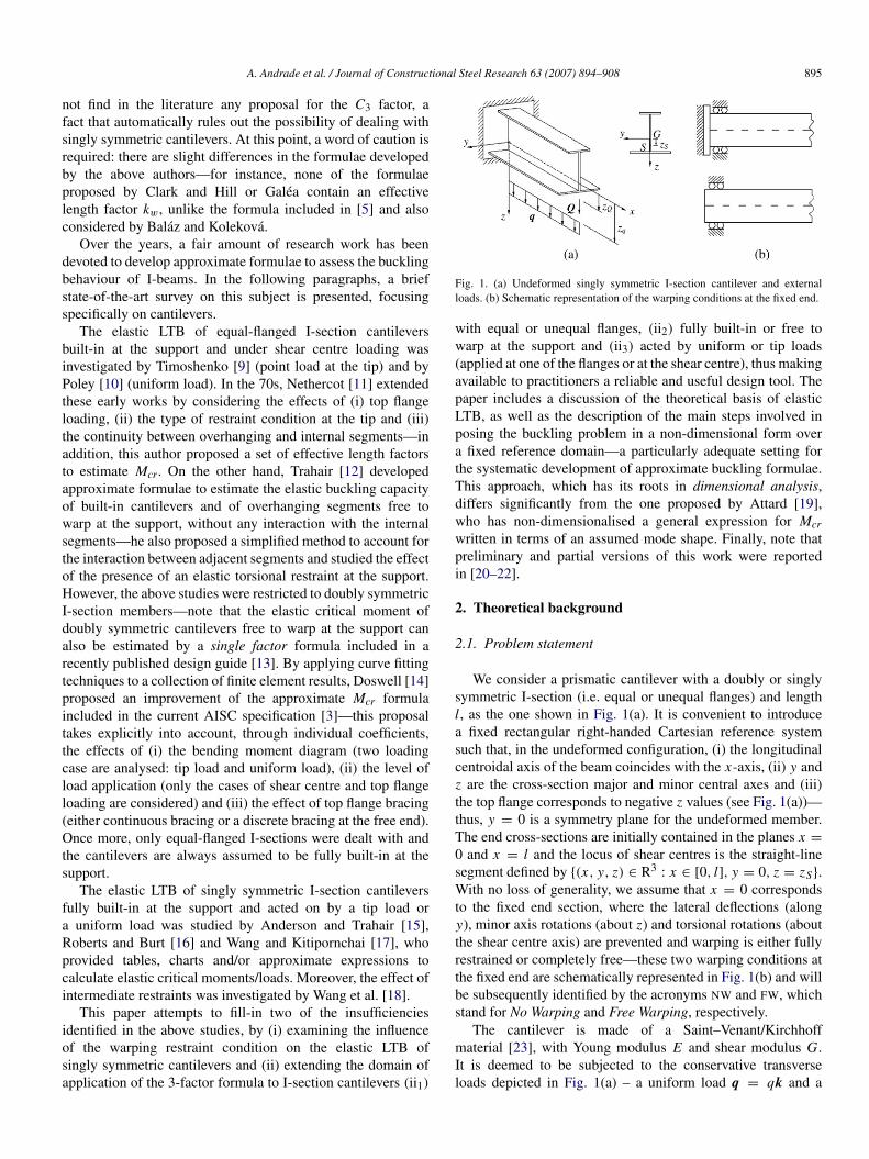
Fig. 1. (a) Undeformed singly symmetric I-section cantilever and externalloads. (b) Schematic representation of the warping conditions at the fixed end.

with equal or unequal flanges, (ii2) fully built-in or free towarp at the support and (ii3) acted by uniform or tip loads(applied at one of the flanges or at the shear centre), thus makingavailable to practitioners a reliable and useful design tool. Thepaper includes a discussion of the theoretical basis of elasticLTB, as well as the description of the main steps involved inposing the buckling problem in a non-dimensional form overa fixed reference domain—a particularly adequate setting forthe systematic development of approximate buckling formulae.This approach, which has its roots in dimensional analysis,differs significantly from the one proposed by Attard [19],who has non-dimensionalised a general expression for Mcrwritten in terms of an assumed mode shape. Finally, note thatpreliminary and partial versions of this work were reportedin [20–22].

2. Theoretical background

2.1. Problem statement

We consider a prismatic cantilever with a doubly or singlysymmetric I-section (i.e. equal or unequal flanges) and lengthl, as the one shown in Fig. 1(a). It is convenient to introducea fixed rectangular right-handed Cartesian reference systemsuch that, in the undeformed configuration, (i) the longitudinalcentroidal axis of the beam coincides with the x-axis, (ii) y andz are the cross-section major and minor central axes and (iii)the top flange corresponds to negative z values (see Fig. 1(a))—thus, y = 0 is a symmetry plane for the undeformed member.The end cross-sections are initially contained in the planes x =

0 and x = l and the locus of shear centres is the straight-linesegment defined by {(x, y, z) ∈ R3

: x ∈ [0, l], y = 0, z = zS}.With no loss of generality, we assume that x = 0 correspondsto the fixed end section, where the lateral deflections (alongy), minor axis rotations (about z) and torsional rotations (aboutthe shear centre axis) are prevented and warping is either fullyrestrained or completely free—these two warping conditions atthe fixed end are schematically represented in Fig. 1(b) and willbe subsequently identified by the acronyms NW and FW, whichstand for No Warping and Free Warping, respectively.

The cantilever is made of a Saint–Venant/Kirchhoffmaterial [23], with Young modulus E and shear modulus G.It is deemed to be subjected to the conservative transverseloads depicted in Fig. 1(a) – a uniform load q = qk and a

896 A. Andrade et al. / Journal of Constructional Steel Research 63 (2007) 894–908

tip load Q = Qk, where k is the unit vector directed alongthe z-axis −, both with the same direction and initially actingon the plane y = 0. Their magnitudes q , Q are assumed tobe proportional to a single factor λ (therefore, we may writeq = q0λ and Q = Q0λ, where q0, Q0 are non-negativereference magnitudes defining the loading profile) and theirconservative character is ensured by the fact that they followthe beam deformation, always remaining parallel to the z-axis.For convenience, we also assume throughout this section thatq0 and Q0 are strictly positive.

It is well-known that such a cantilever is prone to lateral-torsional buckling, a bifurcation-type of instability (from theLatin word bifurcus—‘with two branches’) where (i) thefundamental path corresponds to equilibrium configurations(parameterised by λ) that are symmetric with respect to theplane y = 0 (i.e. the cantilever is subjected solely to majoraxis bending) and (ii) the buckled states are associated withnon-symmetric configurations—the cantilever deflects laterally,along y, and twists. This phenomenon is an obvious instanceof symmetry breaking. However, not all symmetry is lost:given any possible buckled state, its reflection upon the planey = 0 is also a possible buckled state—i.e. instability breaksthe symmetry of the equilibrium configuration, but not thesymmetry of the solution set.

In this section, we aim at formulating the problemof identifying the bifurcation points along the cantilever’sfundamental path in a way that is well suited for thesystematic development of approximate buckling formulae. Inorder to linearise the problem, we neglect the pre-bucklingflexural deflections, thus assuming that the cantilever remainsstraight up until the onset of buckling—in design, it isprudent to disregard the beneficial effect of pre-bucklingdeflections because (i) it may be significantly reduced, oreven fully removed, by any pre-cambering of the memberand (ii) it depends heavily on the actual conditions of lateralrestraint [24]. Moreover, the analysis is carried out under theassumption of small strains.

2.2. Mathematical modelling

Using Vlassov’s classical thin-walled beam theory hypothe-ses [25] – the cross-sections do not deform in their own planeand the shear strains on the mid-surface are negligible −, it ispossible to show that the second variation, from a given funda-mental state, of the cantilever total potential energy Π is definedby (e.g., [26])

δ2Π =E Iz

2

∫ l

0v2,xx dx +

G It

2

∫ l

0φ2,x dx +

E Iw2

∫ l

0φ2,xx dx

+12

∫ l

0M f

y (2v,xxφ + βyφ2,x )dx +

12(zq − zS)q

×

∫ l

0φ2dx +

12(zQ − zS)Qφ(l)2, (1)

where (i) v(x) and φ(x) are variations of V (x, λ) (shearcentre displacement along y) and Φ(x, λ) (rotation about theundeformed shear centre axis), which are independent from λ

(recall that V and Φ are both identically zero in the fundamentalstate), (ii) Iz, It and Iw are standard geometrical propertiesof the undeformed cross-section, (iii) βy is a cross-sectionalasymmetry property, defined by

βy =1Iy

∫A

z( y2+ z2)dA − 2zS, (2)

(iv) M fy denotes the bending moment distribution in the

fundamental state, given by

M fy (x, λ) = −

(12

q0 (l − x)2 + Q0 (l − x))λ

= M fy0(x)λ, (3)

where M fy0 is a function of x alone and denotes the bending

moment diagram caused by the reference loads q0k and Q0k,and (v) zq and zQ identify the point of load application—see Fig. 1(a). In the sequel, we exclude the limiting cases ofT, inverted T and narrow rectangular cross-sections, so as toensure that Iw 6= 0.

In order to completely define the functional δ2Π , it isnecessary to specify the class of admissible functions v andφ. There are two properties that must be characterised: (i) thesmoothness required of these functions and (ii) the boundaryconditions they must satisfy. The integrals in (1) only makesense if v and φ are square-integrable in (0, l) and possesssquare-integrable first and second derivatives. In addition, theadmissible functions v and φ must satisfy the homogeneousform of the essential (Dirichlet) boundary conditions, i.e.

v(0) = 0 v,x (0) = 0 φ(0) = 0 φ, x (0) = 0, (4)

the last one applying only if warping is prevented at the fixedend section (NW). The real-valued functions fulfilling the aboverequirements are termed kinematically admissible.

According to Trefftz’s criterion [27,28] – for a criticalappraisal of this criterion, together with a brief historicalaccount and references to its application, the interested reader isreferred to [29] –, the variational form of the buckling problemcan be stated as follows:

Problem A (Variational Form). Find real scalars λ andkinematically admissible functions v, φ 6= 0 rendering δ2Πstationary, i.e. satisfying the variational condition

δ (δ2Π ) = 0. (5)

Applying standard Calculus of Variations techniques [30],we obtain the classical or strong form of Problem A, whichmay be phrased as follows:

Problem A (Strong Form). Find λ ∈ R and real-valuedfunctions v, φ ∈ C4([0, l]), with v, φ 6= 0, satisfying thedifferential equations

E Izv,xxxx +

(M f

y0φ),xxλ = 0 (6)

(M fy0v,xx + q0(zq − zS)φ − βy(M

fy0φ,x ),x )λ− G Itφ,xx

+ E Iwφ,xxxx = 0 (7)


in (0, l) (Euler–Lagrange equations of δ2Π ) and the boundaryconditions

v(0) = 0 Q0φ(l)λ+ E Izv,xxx (l) = 0 (8)v,x (0) = 0 E Izv,xx (l) = 0 (9)φ(0) = 0 (zQ − zS)Q0φ(l)λ+ G Itφ,x (l)

− E Iwφ,xxx (l) = 0 (10)φ,x (0) = 0 (NW) or E Iwφ,xx (0) = 0 (FW)

E Iwφ,xx (l) = 0. (11)

Due to the regularity of the data – constant mechanical andgeometrical properties and M f

y0 ∈ C∞([0, l]) –, the strong andvariational forms of the problem are equivalent.

From a mathematical viewpoint, Problem A is aneigenvalue problem—the elastic bifurcation load factors andthe corresponding buckling modes are its eigenvalues andeigenfunctions. Given the self-adjoint character of this problem,all eigenvalues are real and the eigenfunctions may be taken tobe real [31,32]—this is the mathematical justification for havingformulated Problem A in terms of real scalars and real functionspaces, in line with its physical nature. The lowest positiveeigenvalue is termed elastic critical load factor and denoted byλcr—accordingly, the corresponding buckling mode (vcr, φcr)

is labelled critical as well. We also speak of the elastic criticalmoment, defined as

Mcr = |M fy (x, λcr)|max = (1/2q0l2

+ Q0l)λcr

= −M fy0(0)λcr.

Integrating twice the field equation (6), together with thenatural (Neumann) boundary conditions (82)–(92), we are ledto the conclusion that v,xx and φ are related by the equation

v,xx = −M f

y0

E Izφλ. (12)

This equation can be viewed as a holonomic kinematicalconstraint [33], which can be used to eliminate v and write thebuckling problem in terms of a single unknown field φ. Indeed,the incorporation of (12) into (7) yields

−M f 2

y0

E Izφλ2

+ (q0(zq − zS)φ − βy(Mf

y0φ,x ),x )λ

− G Itφ,xx + E Iwφ,xxxx = 0 (13)

and Problem A may then be replaced by the following one,which takes on the form of a quadratic eigenvalue problem:

Problem B (Strong Form). Find λ ∈ R and φ ∈ C4([0, l]),with φ 6= 0, satisfying the field equation (13) and the boundaryconditions (10) and (11).

It is obvious that a variational characterisation can be given forProblem B: it suffices to introduce (12) into (1) and to consideragain Eq. (5). If required, v can be obtained through themere integration of Eq. (12) subjected to the initial conditions(81)–(91).

2.3. Equivalent scaled problems

By an appropriate change of variable and subsequent scalingof the functions v and φ, Problems A and B may be transformedinto equivalent ones, posed in a fixed reference domain(i.e. independent of the cantilever length l) and written in a non-dimensional form—this is most convenient because it enablesa general and systematic representation of the cantilever LTBbehaviour.

Since the interval [0, 1] is taken as the fixed referencedomain, the associated change of variable is defined by thestretch ξ : [0, l] → [0, 1], ξ = x/ l. Moreover, we introducethe scaled non-dimensional functions v : [0, 1] → R, v(ξ) =√

E Iz/(G It )v(ξ l)/ l and φ : [0, 1] → R, φ(ξ) = φ(ξ l). Then,the strong form of the scaled versions of Problems A and B maybe stated as follows:

Problem C (Strong Form). Find λ ∈ R and v, φ ∈ C4([0, 1]),with v, φ 6= 0, satisfying the differential equations

v,ξξξξ + (µf0 φ),ξξλ = 0 (14)

(µf0 v,ξξ + 2εqγqφ − δy(µ

f0 φ,ξ ),ξ )λ− φ,ξξ

+K 2

π2 φ,ξξξξ = 0 (15)

in (0, 1) and the boundary conditions

v(0) = 0 γQφ(1)λ+ v,ξξξ (1) = 0 (16)v,ξ (0) = 0 v,ξξ (1) = 0 (17)

φ(0) = 0 εQγQφ(1)λ+ φ,ξ (1)−K 2

π2 φ,ξξξ (1) = 0 (18)

φ,ξ (0) = 0 (NW) or φ,ξξ (0) = 0 (FW) φ,ξξ (1) = 0,(19)

where

µf0 (ξ) =

l√

E IzG ItM f

y0(ξ l)

= −(1 − ξ)((1 − ξ)γq + γQ) (20)

and

γq =q0l3

2√

E IzG ItγQ =

Q0l2√

E IzG ItK =

π

l

√E IwG It

(21)

δy =βy

l

√E Iz

G Itεq =

zq − zS

l

√E Iz

G It

εQ =zQ − zS

l

√E Iz

G It(22)

are non-dimensional parameters, very much identical to theones proposed by Anderson and Trahair [15].

Problem D (Strong Form). Find λ ∈ R and φ ∈ C4([0, 1]),with φ 6= 0, satisfying the differential equation

−µf 20 φλ2

+ (2εqγqφ − δy(µf0 φ,ξ ),ξ )λ− φ,ξξ

+K 2

π2 φ,ξξξξ = 0 (23)


in (0, 1) and the boundary conditions

φ(0) = 0 εQγQφ(1)λ+ φ,ξ (1)−K 2

π2 φ,ξξξ (1) = 0 (24)

φ,ξ (0) = 0 (NW) or φ,ξξ (0) = 0 (FW) φ,ξξ (1) = 0. (25)

Again, it is readily seen that an equivalent variationalcharacterisation can be provided for Problems C and D. Forinstance, (14) and (15), (162), (172), (182), (192) and (191) (thelast one only if the fixed end section is free to warp—FW) arethe Euler–Lagrange equations and natural boundary conditionsrelated to the vanishing of the first variation of the functional

δ2Π =12

∫ 1

0v2,ξξdξ +

12

∫ 1

0φ

2,ξdξ +

K 2

2π2

∫ 1

0φ

2,ξξdξ

+

(12

∫ 1

0µ

f0

(2v,ξξφ + δyφ

2,ξ

)dξ + εqγq

∫ 1

0φ

2dξ

+12εQγQφ(1)2

)λ, (26)

whose admissible arguments v, φ (i) lie in the space of square-integrable functions in (0, 1) with equally square-integrable firstand second derivatives and (ii) satisfy (161), (171), (181) and,when warping is prevented at the fixed end section (NW), also(191)—note that

δ2Π =l

G Itδ2Π . (27)

Once λcr has been obtained, the elastic critical moment isgiven simply by

Mcr =

√E IzG It

l(γq + γQ)λcr. (28)

From either of the above two problems, we conclude that“cantilever families” sharing the same (i) K , δy, εq , εQ andq0l/Q0 values and (ii) warping restraint condition at thefixed end (NW or FW) exhibit identical values of γqλ orγQλ at buckling. In other words, the cantilevers belonging tosuch “families” are similar, as far as the LTB behaviour isconcerned—thus, γqλcr or γQλcr can be written as functionsof K , δy , εq , εQ and q0l/Q0.

It is worth pointing out that the same conclusion can bereached through the use of Buckingham’s π -theorem [34],which summarises the entire theory of dimensional analysis—Buckingham himself did not rigorously prove the theoremthat bears his name, although he presented evidence makingits validity seem plausible (a proof of this theorem can befound, for instance, in [35]). On the basis of a purely physical(i.e. phenomenological) reasoning, the following unspecifiedfunctional relationship, involving n = 9 quantities, may bestated:

Mcr = f(

E Iz,G It , E Iw, βy, l, (zq−zS), (zQ−zS),q0lQ0

).(29)

The rank of the associated dimensional matrix is r = 3and Buckingham’s π -theorem asserts that (29) can be written

in terms of a complete set of n − r = 6 non-dimensionalparameters:

π1 = g(π2, π3, π4, π5, π6). (30)

There is an infinite number of different complete sets of non-dimensional parameters. One possible choice is π1 = γqλcr(or, alternatively, π1 = γQλcr), π2 = K , π3 = δy, π4 =

εq , π5 = εQ and π6 = q0l/Q0, which arises naturally duringthe manipulation of the governing equations.

It should be stressed that, up to this point, the shape ofthe cross-section has not yet been invoked in any of thederivations. Thus, all the previous results are valid for thin-walled cantilevers with arbitrary singly symmetric open cross-sections under major axis bending.

Since the parameters K , δy, εq , εQ do not convey a clearperception of the cantilever slenderness, asymmetry and loadposition, we adopt a new set of non-dimensional parameters,which (i) apply specifically to I-section beams and (ii) areclosely related to the geometrical and mechanical propertiesgoverning their LTB behaviour. They are similar to the onesproposed by Kitipornchai and Trahair [36] and given by

K =π

l

√E Izh2

S4G It

ψ f =Ib f − It f

Ib f + It fζq = 2

zq − zS

hS

ζQ = 2zQ − zS

hS,

(31)

where hS is the distance between the flange mid-lines and Ibfand Itf are the moments of inertia, about the z-axis, of thebottom and top flanges. It is worth noting that:

(i) The parameter ψ f (i1) is purely geometrical (i.e. inde-pendent of the M f

y sign), unlike the ones defined in [5,37], (i2) provides an easy-to-feel measure of the flangeasymmetry and (i3) varies from ψ f = −1 (T-section) toψ f = 1 (inverted T-section), with ψ f = 0 for an equalflanged I-section. It is related to the warping constant Iwthrough [36,37]

Iw = (1 − ψ2f )Izh2

S/4 (32)

and may also be used to approximate βy by means of [37]

βy ≈{−0.8ψ f hS if ψ f > 0 (i.e. favourable flange asymmetry)−ψ f hS if ψ f < 0 (i.e. unfavourable flange asymmetry)

(33)

(note that βy obviously vanishes for an equal flangedI-section). An assessment of the errors involved in theapproximation (33) and in the subsequent evaluation ofγqλcr and γQλcr is presented in an appendix at the endof this paper.

(ii) In commonly used I-section cantilevers, the beamparameter K ranges from 0.1 to 2.5 [17,36]. Low (high)K values mean long (short) cantilevers and/or compact(slender) cross-sections. Furthermore, one has K = K foran equal flanged cantilever (ψ f = 0).

(iii) The load position parameters ζq and ζQ enable an easyvisualisation of the location of the load point of application


along the cross-section height (or, to be exact, its locationin between the flange mid-lines). Typical values of theseparameters are (iii1) ζq(Q) = 0 (load applied at the shearcentre), (iii2) ζq(Q) = −(1 + ψ f ) (load applied at the topflange centroid) and (iii3) ζq(Q) = 1 −ψ f (load applied atthe bottom flange centroid) [17].

(iv) Since the set {K , δy, εq , εQ} can be uniquely determinedfrom {K , ψ f , ζq , ζQ} by means of the expressions

K = K√

1 − ψ2f εq (Q) =

1π

K ζq (Q) (34)

δy ≈

−

2 × 0.8π

ψ f K if ψ f > 0

−2πψ f K if ψ f < 0,

(35)

the latter can also be used to write the governing equationsin non-dimensional form.

3. Numerical implementation

The application of a structure-preserving discretisationmethod (such as the methods of Rayleigh–Ritz and Bubnov–Galerkin) to Problem D generates an algebraic quadraticeigenvalue problem of the form

(A + λB + λ2C)x = 0, (36)

where A, B and C are real symmetric matrices (of order n,say)—A and C are positive and negative definite, respectively.In the case of small-to-moderate n, the standard approachto solve (36) numerically involves its linearisation, i.e. itsconversion into an equivalent linear generalised eigenproblemby means of an augmentation procedure resembling thereduction of a second-order linear differential equation to asystem of two first-order ones [38,39]. In practice, the mostcommonly used linearisations involve one of the companionforms[

0 N−A −B

] [xu

]= λ

[N 00 C

] [xu

](37)

[−A 00 N

] [xu

]= λ

[B CN 0

] [xu

], (38)

where N is any non-singular n × n real matrix and u = λx.This approach has two major drawbacks: (i) the dimension ofthe linearised problem is twice that of the original quadratic oneand (ii) backward stability cannot always be guaranteed for thequadratic problem, even if a backward stable algorithm is usedto solve the linearised problem [40].

Therefore, we opted for the discretisation of Problem C,leading directly to an algebraic linear generalised eigenproblemof the form

Gx =1λ

Kx, (39)

where G and K are real symmetric matrices and K ispositive definite. Then, it is possible to perform the Cholesky

factorisation of K (K = LLT, where L stands for a lowertriangular matrix with positive diagonal entries) and reduce (39)to the standard symmetric form

(L−1GL−T)y =1λ

y, (40)

where y = LTx. The standard problem (40) can be solved by thesymmetric QR algorithm (e.g., [41]) or any other eigensolverfor real symmetric matrices.

The discretisation scheme employed in this work is theRayleigh–Ritz method, named after Strutt, 3rd Baron Rayleigh,and Ritz [42,43]—for a comprehensive analysis of the methodand a broad discussion of its application areas, see works byMikhlin [32,44]. The functions v and φ were approximated bythe sequences of linear combinations of coordinate functions

vn(ξ) =

n∑k=1

a(n)k

[1 − cos

((2k − 1)π

2ξ

)]n = 1, 2, . . . (41)

φn(ξ) =

n∑k=1

b(n)k

[1 − cos

((2k − 1)π

2ξ

)]n = 1, 2, . . . (NW) (42)

φn(ξ) = b(n)1 ξ +

n∑k=2

b(n)k sin ((k − 1)πξ)

n = 1, 2, . . . (FW), (43)

where the superscript in the coefficients a(n)k , b(n)k stresses theirdependence on n. Since the same number n of terms is usedto approximate v and φ, one is led to a discrete problemwith 2n degrees of freedom—note also that (43) satisfies thenatural boundary condition (191). The numerical procedure wascontinued until the relative differences between the bucklingcapacities γqλcr or γQλcr computed with three consecutivevalues of n did not exceed 0.1%—it was found that this criterioncould always be satisfied by considering up to nine terms(n ≤ 9) in (41)–(43).

4. Parametric study

A parametric study was conducted to determine the non-dimensional elastic buckling capacities γqλcr or γQλcr ofI-section cantilevers and the associated normalised bucklingmode shapes φcr as a function of the beam parameter K (0.1 ≤

K ≤ 2.5), for (i) selected values of the flange asymmetryparameter ψ f (in the range −0.8 ≤ ψ f ≤ 0.8) and (ii) threeload positions (shear centre, top and bottom flange centroids).The cantilevers were acted on by a uniform load or a tip load(i.e. Q0 = 0 or q0 = 0)—the simultaneous application of thetwo loads was not considered in this work. As discussed earlier,warping at the fixed end section was either fully prevented (NW)or completely free (FW).

The numerical results were compared with values reportedby (i) Wang and Kitipornchai [17], for cantilevers with nowarping at the fixed end and both equal and unequal flanges,and by (ii) Trahair [12], for cantilevers free to warp at the fixed


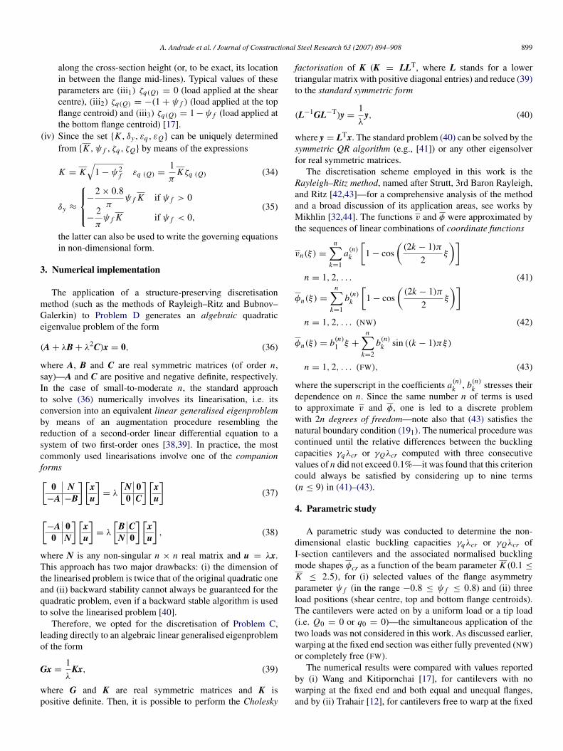
Fig. 2. Cantilevers acted on by a uniform load applied at the top flange centroid (ζq = −1 − Ψ f ): variation of γqλcr with K and Ψ f .

Fig. 3. Cantilevers acted on by a uniform load applied at the shear centre (ζq = 0): variation of γqλcr with K and Ψ f .

end and equal flanges—to the best of our knowledge, no Mcrvalues for cantilevers with unequal flanges and free to warpat the fixed end are available in the literature. An excellentagreement was found in all cases.

Figs. 2–7 show plots of the elastic buckling capacities γqλcr

and γQλcr against the beam parameter K , for selected values ofthe flange asymmetry parameterψ f and the three load positionsconsidered. These plots show that:

(i) As expected, the cantilevers restrained from warping atthe fixed end (NW) exhibit higher buckling capacities thanthe ones that are free to warp at that section (FW). Whilethe difference is only marginal for very low values of K ,it gradually increases with this parameter and becomessubstantial for high K values. This indicates that thebuckling capacity of a cantilever restrained from warpingat the support and having a high K depends, to a large

extent, on the warping torsion generated during buckling—this effect is hardly mobilised in the absence of an externalwarping restraint. On the other hand, the warping torsion isnot relevant in cantilevers with very low K , which impliesthat the warping restraint at the support has little impact onγqλcr or γQλcr.

(ii) Although the plots concerning cantilevers subjected touniform and tip loads display similar qualitative features,the γqλcr values are always higher: for equal end values (atξ = 0 and ξ = 1), the magnitude of the non-dimensionalbending moment distribution |µ

f0 (ξ)λ| associated with the

uniform load is smaller at any given interior point (0 <

ξ < 1).(iii) The so-called Wagner’s effect [15,45], which may be

viewed as an increase (reduction) in the actual torsionalrigidity of the cross-sections when the compression


Fig. 4. Cantilevers acted on by a uniform load applied at the bottom flange centroid (ζq = 1 − Ψ f ): variation of γqλcr with K and Ψ f .

Fig. 5. Cantilevers acted on by a tip load applied at the top flange centroid (ζQ = −1 − Ψ f ): variation of γQλcr with K and Ψ f .

flange is larger (smaller) than the tension one, is clearlynoticeable for the cantilevers loaded at the shear centre:both γqλcr and γQλcr increase monotonically with ψ f .

(iv) In the cantilevers loaded at the top or bottom flange, thevariation of the buckling capacity with ψ f stems fromthe interplay between (iv1) Wagner’s effect and (iv2)

the location of the point of load application relative tothe shear centre—recall that, for top or bottom flangeloading, the value of the parameters ζq and ζQ dependson ψ f . This explains why, in some cases, this variationis not monotonic (e.g., warping restrained cantilevers withψ f > 0 and bottom flange loading). It is also worth notingthat, for top flange loading and moderate-to-high K values,the maximum buckling capacity occurs for sections withequal (or nearly equal) flanges.

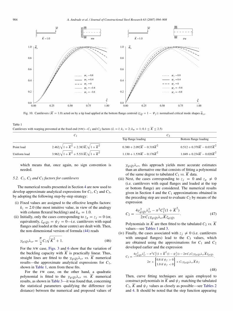
The critical buckling mode shapes φcr of cantilevers withK = 1.0 and acted on by tip loads are shown in Figs. 8–10(these shapes are normalised so that φcr max = 1)—since thebuckling mode shapes of the cantilevers subjected to uniformloads are qualitatively similar, they are not presented here. Themost striking difference between the two graphs in each ofthese figures concerns the shape of the critical modes near thesupported end—while the cantilevers prevented from warpingat the support (NW) display a considerable curvature, the onesthat are free to warp (FW) exhibit a linear ascending branch,which is an immediate consequence of the natural boundarycondition φ,ξξ (0) = 0. It is also interesting to note that, inthe cases of shear centre and top flange loading, φcr increasesmonotonically with ξ , so that the maximum torsional rotationoccurs at the cantilever free end. Conversely, for bottom flange


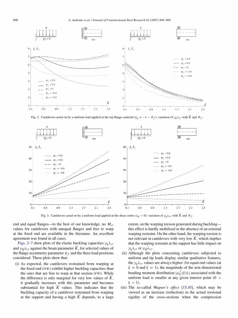
Fig. 6. Cantilevers acted on by a tip load applied at the shear centre (ζQ = 0): variation of γQλcr with K and Ψ f .

Fig. 7. Cantilevers acted on by a tip load applied at the bottom flange centroid (ζQ = 1 − Ψ f ): variation of γQλcr with K and Ψ f .

loading the critical mode shapes reach a maximum for ξ < 1and then decrease towards the cantilever free end, a feature thatbecomes gradually more significant as the value of the flangeasymmetry parameter ψ f diminishes.

5. Approximate formulae to estimate elastic criticalmoments

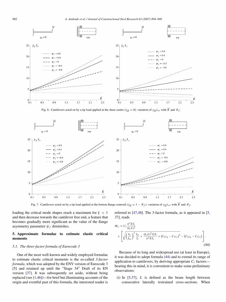
5.1. The three-factor formula of Eurocode 3

One of the most well-known and widely employed formulaeto estimate elastic critical moments is the so-called 3-factorformula, which was adopted by the ENV version of Eurocode 3[5] and retained up until the “Stage 34” Draft of its ENversion [37]. It was subsequently set aside, without beingreplaced (see [1,46])—for brief but illuminating accounts of theorigin and eventful past of this formula, the interested reader is

referred to [47,48]. The 3-factor formula, as it appeared in [5,37], reads

Mcr = C1π2 E Iz

(kz L)2

×

√( kz

kw

)2 IwIz

+(kz L)2 G It

π2 E Iz+(C2zg − C3z j

)2−(C2zg − C3z j

) .(44)

Because of its long and widespread use (at least in Europe),it was decided to adopt formula (44) and to extend its range ofapplication to cantilevers, by deriving appropriate Ci factors—bearing this in mind, it is convenient to make some preliminaryobservations:

(i) In [5,37], L is defined as the beam length betweenconsecutive laterally restrained cross-sections. When


Fig. 8. Cantilevers (K = 1.0) acted on by a tip load applied at the top flange centroid (ζQ = −1 − Ψ f ): normalised critical mode shapes φcr .

Fig. 9. Cantilevers (K = 1.0) acted on by a tip load applied at the shear centre (ζQ = 0): normalised critical mode shapes φcr .

dealing with cantilevers, this definition has to be modifiedand, therefore, we take L as the cantilever length—recallthat it was previously denoted in this paper by the lowercase letter l.

(ii) According to [5,37], the Ci factors depend only on(ii1) the bending moment diagram and (ii2) the endrestraint conditions. However, it has been recognised byseveral authors (e.g., [13,47,49]) that, except in a fewparticular cases, these factors also depend on (ii1) thebeam parameter K , (ii2) the location of the point of loadapplication (C2,C3) and (ii3) the degree of cross-sectionasymmetry with respect to the y-axis (C3).

(iii) The quantities kz and kw are effective length factors,the former associated with the end rotations about thez-axis and the latter with the end warping restraint. Itshould be noticed that these factors (iii1) are not properly

defined (there is no direct relation to the distance betweeninflection points of the critical buckling mode shape{vcr, φcr}) and (iii2) do not fully account for the endsupport conditions—indeed, when kz changes so do the Cifactors. Thus, the values assigned to kz and kw should beregarded as merely conventional.

(iv) For gravity loads, we define zg = −(zq(Q) − zS), whichmeans that one has zg > 0 for loads applied above theshear centre and there is no need for any sign convention—incidentally, the convention adopted in [37] is incorrect.Moreover, it should be made clear that formula (44) isnot valid when the beam is subjected to transverse loadsapplied at different levels (e.g., if one has zq 6= zQ).

(v) The cross-sectional property z j is defined as

z j = zS −1

2Iy

∫A

z(y2+ z2)dA = −

βy

2, (45)


Fig. 10. Cantilevers (K = 1.0) acted on by a tip load applied at the bottom flange centroid (ζQ = 1 − Ψ f ): normalised critical mode shapes φcr .

Table 1Cantilevers with warping prevented at the fixed end (NW)—C1 and C2 factors (L = l; kz = 2; kw = 1; 0.1 ≤ K ≤ 2.5)

C1 C2Top flange loading Bottom flange loading

Point load 2.462/√

1 + K 2+ 2.383K/

√1 + K 2 0.380 + 2.092K − 0.318K 2 0.512 + 0.370K − 0.033K 2

Uniform load 3.962/√

1 + K 2+ 5.531K/

√1 + K 2 1.130 + 1.539K − 0.176K 2 1.049 + 0.234K − 0.020K 2

which means that, once again, no sign convention isneeded.

5.2. C1,C2 and C3 factors for cantilevers

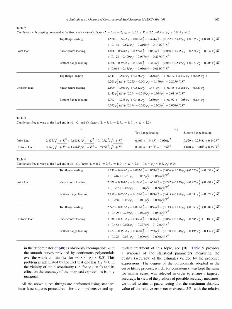
The numerical results presented in Section 4 are now used todevelop approximate analytical expressions for C1, C2 and C3,by adopting the following step-by-step strategy:

(i) Fixed values are assigned to the effective lengths factors:kz = 2.0 (the most intuitive value, in view of the analogywith column flexural buckling) and kw = 1.0.

(ii) Initially, only the cases corresponding to zg = z j = 0 (or,equivalently, ζq(Q) = ψ f = 0—i.e. cantilevers with equalflanges and loaded at the shear centre) are dealt with. Then,the non-dimensional version of formula (44) reads

γq(Q)λcr =π

2C1

√K

2+ 1. (46)

For the NW case, Figs. 3 and 6 show that the variation ofthe buckling capacity with K is practically linear. Thus,straight lines are fitted to the γq(Q)λcr vs. K numericalresults—the approximate analytical expressions for C1,shown in Table 1, stem from these fits.

For the FW case, on the other hand, a quadraticpolynomial is fitted to the γq(Q)λcr vs. K numericalresults, as shown in Table 3—it was found that, concerningthe statistical parameters qualifying the difference (ordistance) between the numerical and proposed values of

γq(Q)λcr, this approach yields more accurate estimatesthan an alternative one that consists of fitting a polynomialof the same degree to tabulated C1 vs. K data.

(iii) Next, the cases corresponding to z j = 0 and zg 6= 0(i.e. cantilevers with equal flanges and loaded at the topor bottom flange) are considered. The numerical resultsgiven in Section 4 and the C1 approximations obtained inthe preceding step are used to evaluate C2 by means of theexpression

C2 =4γ 2

q(Q)λ2cr − π2C2

1(1 + K2)

2πC1γq(Q)λcr K ζq(Q). (47)

Polynomials in K are then fitted to the tabulated C2 vs. Kvalues—see Tables 1 and 3.

(iv) Finally, the cases associated with z j 6= 0 (i.e. cantileverswith unequal flanges) lead to the C3 values, whichare obtained using the approximations for C1 and C2developed earlier and the expression

C3 =4γ 2

q(Q)λ2cr − π2C2

1 (1 + K2(1 − ψ2

f ))− 2πC1C2γq(Q)λcr K ζq(Q)

2π ×

{0.8 if ψ f > 0

1.0 if ψ f < 0

}× C1γq(Q)λcr Kψ f

.

(48)

Then, curve fitting techniques are again employed toconstruct polynomials in K and ψ f matching the tabulatedC3, K and ψ f values as closely as possible—see Tables 2and 4. It should be noted that the step function appearing


Table 2Cantilevers with warping prevented at the fixed end (NW)—C3 factor (L = l; kz = 2; kw = 1; 0.1 ≤ K ≤ 2.5; −0.8 ≤ ψ f ≤ 0.8, ψ f 6= 0)

Top flange loading 1.520 − 1.342ψ f − 0.010ψ2f − 0.424ψ3

f + (0.162 + 2.419ψ f + 0.875ψ2f + 0.400ψ3

f )K

+ (0.148 − 0.623ψ f − 0.216ψ2f + 0.141ψ3

f )K2

Point load Shear centre loading 1.808 − 0.944ψ f + 0.299ψ2f − 0.061ψ3

f + (0.060 + 1.235ψ f − 0.574ψ2f − 0.337ψ3

f )K

+ (0.128 − 0.409ψ f + 0.047ψ2f + 0.237ψ3

f )K2

Bottom flange loading 1.966 − 0.792ψ f + 0.139ψ2f − 0.341ψ3

f + (0.061 + 0.549ψ f + 0.077ψ2f − 0.206ψ3

f )K

+ (0.064 − 0.135ψ f − 0.050ψ2f + 0.058ψ3

f )K2

Top flange loading 2.441 − 1.589ψ f + 0.176ψ2f − 0.658ψ3

f + (−0.412 + 2.442ψ f + 0.635ψ2f +

0.261ψ3f )K + (0.273 − 0.601ψ f − 0.140ψ2

f + 0.205ψ3f )K

2

Uniform load Shear centre loading 2.609 − 1.801ψ f + 0.522ψ2f + 0.461ψ3

f + (−0.445 + 2.251ψ f − 0.620ψ2f −

1.443ψ3f )K + (0.244 − 0.710ψ f + 0.044ψ2

f + 0.611ψ3f )K

2


f + (−0.492 + 1.008ψ f − 0.134ψ2f −

0.095ψ3f )K + (0.194 − 0.263ψ f − 0.003ψ2

f + 0.060ψ3f )K

2

Table 3Cantilevers free to warp at the fixed end (FW)—C1 and C2 factors (L = l; kz = 2; kw = 1; 0.1 ≤ K ≤ 2.5)

C1 C2Top flange loading Bottom flange loading

Point load 2.437/√

1 + K 2+ 0.613K/

√1 + K 2

− 0.105K 2/

√1 + K 2 0.409 + 1.444K + 0.070K 2 0.529 + 0.234K + 0.149K 2

Uniform load 3.840/√

1 + K 2+ 1.496K/

√1 + K 2

− 0.247K 2/

√1 + K 2 0.987 + 1.420K + 0.165K 2 1.028 + 0.388K + 0.150K 2

Table 4Cantilevers free to warp at the fixed end (FW)—C3 factor (L = l; kz = 2; kw = 1; 0.1 ≤ K ≤ 2.5; −0.8 ≤ ψ f ≤ 0.8, ψ f 6= 0)

Top flange loading 1.732 − 0.648ψ f − 0.062ψ2f + 0.059ψ3

f + (0.066 + 1.539ψ f + 0.520ψ2f − 0.032ψ3

f )K

+ (0.446 + 0.221ψ f − 0.037ψ2f + 0.066ψ3

f )K2

Point load Shear centre loading 2.021 + 0.361ψ f + 0.176ψ2f − 0.655ψ3

f + (0.242 + 0.120ψ f − 0.426ψ2f + 0.891ψ3

f )K

+ (0.337 + 0.052ψ f − 0.198ψ2f − 0.099ψ3

f )K2


f + (0.435 + 0.168ψ f − 0.083ψ2f − 0.077ψ3

f )K

+ (0.238 − 0.022ψ f − 0.011ψ2f − 0.030ψ3

f )K2

Top flange loading 2.669 − 0.815ψ f + 0.071ψ2f − 0.066ψ3

f + (0.113 + 1.812ψ f + 0.359ψ2f + 0.007ψ3

f )K

+ (0.499 + 0.289ψ f + 0.043ψ2f + 0.081ψ3

f )K2

Uniform load Shear centre loading 3.036 + 0.310ψ f + 0.306ψ2f − 0.888ψ3

f + (0.066 + 0.036ψ f − 0.585ψ2f + 1.180ψ3

f )K

+ (0.462 + 0.098ψ f − 0.227ψ2f − 0.123ψ3

f )K2


f + (0.190 + 0.348ψ f − 0.195ψ2f − 0.137ψ3

f )K

+ (0.395 − 0.071ψ f − 0.009ψ2f + 0.009ψ3

f )K2

in the denominator of (48) is obviously incompatible withthe smooth curves provided by continuous polynomialsover the whole domain (i.e. for −0.8 ≤ ψ f ≤ 0.8). Thisproblem is attenuated by the fact that one has C3 ≈ 0 inthe vicinity of the discontinuity (i.e. for ψ f ≈ 0) and itseffect on the accuracy of the proposed expressions is onlymarginal.

All the above curve fittings are performed using standardlinear least squares procedures—for a comprehensive and up-

to-date treatment of this topic, see [50]. Table 5 providesa synopsis of the statistical parameters measuring thequality (accuracy) of the estimates yielded by the proposedexpressions. The degree of the polynomials adopted in thecurve fitting process, which, for consistency, was kept the samefor similar cases, was selected in order to ensure a targetedaccuracy. In view of the plethora of possible accuracy measures,we opted to aim at guaranteeing that the maximum absolutevalue of the relative error never exceeds 5%, with the relative


Table 5Statistical parameters

Top flange loading Shear centre loading Bottom flange loading

NW

Point load

σerr 0.01068 0.00897 0.00792err (%) 0.082 0.105 0.111r2 0.99664 0.99985 0.99987|err| (%) 0.808 0.655 0.531max|err| (%) 4.021 3.365 3.687(|err| > 2.5%) (%) 3 3 4

Uniform load


FW

Point load


Uniform load


error defined as

err =

(γq(Q)λcr

)num −

(γq(Q)λcr

)app(

γq(Q)λcr)

num

(49)

(as shown in Table 5, this criterion is only violated onceand by a very minute margin). Table 5 includes (i) thestandard deviation σerr and mean value err of the relative errordistribution, (ii) the square of the correlation coefficient r(also known as product-moment correlation coefficient orPearson’s correlation coefficient), (iii) the more significant,from a practical viewpoint, mean of the absolute values of therelative error |err|, (iv) the maximum absolute value of therelative error and (v) the number of cases, in percentage, withabsolute values of the relative error greater than 2.5%—thisnumber is always rather small, with the majority of the casesoccurring for K ≈ 0.1).

6. Conclusions

The so-called 3-factor formula (included, for instance, inthe ENV version of Eurocode 3 [5]) is one of the mostcommonly used general formulae to estimate elastic criticalmoments in steel beams prone to LTB. In this paper, thedomain of application of this formula is extended to cantilevers,by providing approximate analytical expressions to determinethe C1, C2 and C3 factors. The paper deals specifically withI-section cantilevers (i) having equal or unequal flanges, (ii)fully built-in or free to warp at the support and (iii) acted on byuniformly distributed or concentrated tip loads (applied eitherat the shear centre or at one of the flanges) and includes a

careful examination of the influence of the warping restraintcondition on the elastic LTB of singly symmetric cantilevers.The estimates yielded by the proposed expressions are veryaccurate: the differences with respect to the numerical (“exact”)results only occasionally exceed 5%.

In summary, our approach consists of the following steps:

(i) write the governing equations in non-dimensional formover a fixed reference domain and, in the process, identifyan adequate complete set of non-dimensional parameters;

(ii) implement numerically (i.e. discretise) the continuummodel stemming from the preceding step;

(iii) perform a parametric study, on the basis of the non-dimensional parameters defined in step (i);

(iv) obtain approximate buckling formulae by fitting amathematical model to the results of the parametric studyusing least squares techniques and qualify quantitativelythe accuracy of the proposed expressions.

The first step of this procedure is of fundamental importance,since it enables a general and systematic representation of thecantilever LTB behaviour, a deeper insight into the nature ofthe phenomenon and a reduction in the number of parametersappearing in the governing equations—this last feature bearsimportant consequences, as far as the time and effort that mustbe put into the parametric study are concerned.

Appendix

The approximation of βy (in terms of ψ f and hS) givenby Eq. (33) is inherent to the results of the parametric studyconcerning singly symmetric I-section cantilevers (Section 4)


and, thus, also to the analytical expressions proposed for the C3factor (Section 5.2).

To assess the accuracy of Eq. (33), a number of HEB and IPEsections, having hS values varying between 166 mm and 484mm, are made singly symmetric through the modification ofone of the flanges, either by reducing its width or by increasingits thickness. The fillets are neglected (i.e. the cross-sectionsare idealised as a combination of three thin rectangles). Theasymmetry parameter ψ f of the modified cross-sections fallswithin the range 0.10 ≤ |ψ f | ≤ 0.95—small-to-moderate|ψ f | values are associated with an increased flange thickness,whereas moderate-to-large |ψ f | values correspond to a reducedflange width. The approximate βy values yielded by Eq. (33)were then compared with the exact ones, as defined by Eq. (2)—this comparison shows that:

1. Eq. (33) always overestimates βy (if ψ f > 0, then βy,exact <

βy,app < 0, while 0 < βy, exact < βy,app if ψ f < 0). Thismeans that an approximate βy value invariably leads to anunderestimation of Mcr.

2. The relative errors (βy,app −βy,exact)/|βy,exact| are generallybelow 15%, even if they occasionally reach almost 20%.However, no obvious correlation appears to exist betweenthe value of |ψ f | and the magnitude of these relative errors.

At this point, what remains to be assessed is how an errorin βy affects the evaluation of Mcr. In order to obtain suchan assessment, we considered the worst-case scenario: a 20%overestimation of βy , regardless of |ψ f |. It was found that:

(i) As expected, the impact of the βy error on Mcr grows with|ψ f | and is more pronounced in the FW case, due to anincreased importance of the Wagner effect in the overallbuckling phenomenon.

(ii) Neither the loading nature (tip point load or uniformlydistributed load) nor its location (shear centre, top orbottom flange) appear to influence the magnitude of theMcr errors significantly, at least in a consistent way.

(iii) As the beam parameter K increases, so does the impactof the βy error on Mcr. In FW cantilevers with highlyasymmetric cross-sections – |ψ f | = 0.8 –, the βy error isfully reflected on the evaluation of Mcr for K = 2.5. As Kdecreases, this impact is slowly (but steadily) attenuated—it does not exceed 10% for K ≤ 0.5.

References

[1] Comite Europeen de Normalisation (CEN). Eurocode 3: Design of steelstructures, Part 1-1: General rules and rules for buildings (EN 1993-1-1).Brussels; 2005.

[2] British Standards Institution (BSI). BS 5950-1: Structural use of steelworkin buildings. Code of practice for design. Rolled and welded sections.London; 2000.

[3] American Institute of Steel Construction (AISC). Manual of steelconstruction—Load and resistance factor design. 3rd ed. Chicago; 2001.

[4] Standards Australia (SA). AS 4100: Steel structures (includingamendments 1, 2 and 3). Homebush; 1990.

[5] Comite Europeen de Normalisation (CEN). Eurocode 3: Design of steelstructures, Part 1-1: General rules and rules for buildings (ENV 1993-1-1).Brussels; 1992.

[6] Clark JW, Hill HN. Lateral buckling of beams. J Struct Div 1960;86(7):175–96.

[7] Galea Y. Abaques de deversement pour profiles lamines. ConstructionMetallique 1981;4:39–51.

[8] Balaz I, Kolekova Y. Factors C1,C2,C3 for computing the elasticcritical moment Mcr . In: Zbornık VI. sympozia Drevo v stavebnychkonstrukciach so zahranicnou ucast’ou, Kocovce. 2004. p. 29–34.

[9] Timoshenko SP. Einige stabilitatsprobleme der elastizitatstheorie. Z MathPhys 1910;58:337–85. Reprinted in The collected papers of Stephen P.Timoshenko. London: McGraw-Hill; 1953.

[10] Poley S. Lateral buckling of cantilevered I-beams under uniform load.Trans ASCE 1956;121:786–90.

[11] Nethercot DA. The effective lengths of cantilevers as governed by lateralbuckling. Struct Eng 1973;51(5):161–8.

[12] Trahair N. Lateral buckling of overhanging beams. In: Morris LJ, editor.Instability and plastic collapse of steel structures. London: Granada; 1983.p. 503–18.

[13] European Commission for Steel and Coal (ECSC). Lateral-torsionalbuckling in steel and composite beams. Research project 7210-PR-183final technical report (Book 2–Design guide). 2003.

[14] Doswell B. Lateral-torsional buckling of wide flange cantilever beams.In: Proc. 2002 annual stability conference. Seattle: Structural StabilityResearch Council; 2002. p. 267–90.

[15] Anderson J, Trahair N. Stability of monosymmetric beams andcantilevers. J Struct Div 1972;98(ST1):269–86.

[16] Roberts TM, Burt CA. Instability of monosymmetric I-beams andcantilevers. Int J Mech Sci 1985;27(5):313–24.

[17] Wang CM, Kitipornchai S. On stability of monosymmetric cantilevers.Eng. Struct. 1986;8(3):169–80.

[18] Wang CM, Kitipornchai S, Thevendran V. Buckling of bracedmonosymmetric cantilevers. Int J Mech Sci 1987;29(5):321–37.

[19] Attard MM. General non-dimensional equation for lateral buckling. Thin-Wall Struct 1990;9(1–4):417–35.

[20] Camotim D, Andrade A. Lateral-torsional buckling of I-sectioncantilevers: Evaluation of critical moments via the EC3 formula. In:Report TC8-2002-023, European convention for constructional steelwork,technical committee 8 (stability) meeting. 2002.

[21] Camotim D, Andrade A. Evaluating critical moments of I-sectioncantilevers via the EC3 formula: Theoretical background and additionalresults. In: Report TC8-2003-007, European convention for constructionalsteelwork, technical committee 8 (stability) meeting. 2003.

[22] Andrade A, Camotim D, Providencia P. Lateral-torsional buckling of steelcantilevers: Evaluation of critical moments using the EC3 Formula. In:Proc. 20th czech and slovak national conference on steel structures andbridges. 2003. p. 635–40.

[23] Ciarlet PG. Mathematical elasticity, vol. 1: Three-dimensional elasticity.Amsterdam: Elsevier; 1988.

[24] Vacharajittiphan P, Woolcock ST, Trahair NS. Effect of in-planedeformation on lateral buckling. J Struct Mech 1974;3(1):29–60.

[25] Vlassov B. Thin-walled elastic bars. Jerusalem: Israel Program forScientific Translations; 1961.

[26] Trahair NS. Flexural-torsional buckling of structures. London: E&FNSpon (Chapman & Hall); 1993.

[27] Trefftz E. Uber die ableitung der stabilitatskriterien des elastischengleichgewichts aus der elastizitatstheorie endlicher deformationen. In:Proc. third intern. congr. appl. mech. vol. 3. 1930. p. 44–50.

[28] Trefftz E. Zur theorie der stabilitat des elastischen gleichgewichts. ZAngew Math Mech 1933;13(2):160–5.

[29] Knops RJ, Wilkes EW. Theory of elastic stability. In: Truesdell C, editor.Mechanics of solids, vol. 3. Berlin: Springer-Verlag; 1984. p. 125–302.Reissue of Encyclopaedia of physics, vol. VIa/3. Berlin: Springer-Verlag;1973.

[30] Mikhlin SG. Mathematical physics, an advanced course. Amsterdam:North-Holland; 1970.

[31] Coddington EA, Levinson N. Theory of ordinary differential equations.New York: McGraw-Hill; 1955.

[32] Mikhlin SG. Variational methods in mathematical physics. Oxford:Pergamon Press; 1964.

[33] Lanczos C. The variational principles of mechanics. Toronto: Universityof Toronto Press; 1970.


[34] Buckingham E. On physically similar systems; illustrations of the use ofdimensional equations. Phys Rev 1914;IV(4):345–76.

[35] Langhaar HL. Dimensional analysis and theory of models. New York:John Wiley & Sons; 1951.

[36] Kitipornchai S, Trahair NS. Buckling properties of monosymmetricI-beams. J Struct Div 1980;106(ST5):941–57.

[37] Comite Europeen de Normalisation (CEN). Eurocode 3: Design of steelstructures, Part 1-1: General rules and rules for buildings (prEN 1993-1-1). Stage 34 draft. Brussels; 2002.

[38] Afolabi D. Linearization of the quadratic eigenvalue problem. ComputStruct 1987;26(6):1039–40.

[39] Tisseur F, Meerbergen K. The quadratic eigenvalue problem. SIAM Rev2001;43(2):235–86.

[40] Tisseur F. Backward error and condition of polynomial eigenvalueproblems. Linear Algebra Appl 2000;309(1–3):339–61.

[41] Golub GH, Van Loan CF. Matrix computations. Baltimore: Johns HopkinsUniversity Press; 1996.

[42] Strutt JW (3rd Baron Rayleigh). The theory of sound, vol. 2. New York:Dover; 1945. Unabridged republication of the second revised and enlargededition of 1894.

[43] Ritz W. Uber eine neue methode zur losung gewisser variationsproblemeder mathematischen physik. J Reine Angew Math 1908;135:1–61.

Reprinted in Gesammelte werke—oeuvres. Paris: Gauthier-Villars,Societe Suisse de Physique; 1911.

[44] Mikhlin SG. The numerical performance of variational methods.Groningen: Wolters-Noordhoff Publishing; 1971.

[45] Wagner H. Torsion and buckling of open sections. NACA technicalmemorandum 807. 1936 [Translation, by Reiss S, of Verdrehung undknickung von offenen profilen, from the 25th Anniversary Number of theTechnische Hochschule; Danzig, 1929. p. 329–43].

[46] Comite Europeen de Normalisation (CEN). Eurocode 3: Design of steelstructures, Part 1-1: General rules and rules for buildings (prEN 1993-1-1). Stage 49 draft, Brussels. 2003.

[47] Balaz I, Kolekova Y. Critical moments of beams and girders—Clark–Mrazik formula. In: Proceedings of the 19th Czech and Slovaknational conference on steel structures and bridges. 2000. p. 87–94.

[48] Braham M. Le deversement elastique des poutres en I a sectionmonosymetrique soumises a un gradient de moment de flexion. ConstrMetall 2001;(1):17–28.

[49] Balaz I, Kolekova Y. Buckling of monosymmetric beams—conjuredproblem (2 parts). In: Proceedings of the 2nd European conference onsteel structures. 1999. p. 701–4. Full paper in CD-ROM.

[50] Bjorck A. Numerical methods for least squares problems. Philadelphia:SIAM; 1996.

on the evaluation of elastic critical moments in doubly ... · on the evaluation of elastic...

Documents