on the effectiveness of single sales … on the effectiveness of single sales factors for state...

1

ON THE EFFECTIVENESS OF SINGLE SALES FACTORS FOR STATE TAXATION

Charles Swenson Professor and Leventhal Research Fellow

Marshall School of Business University of Southern California

June, 2011

ABSTRACT This study models and empirically tests the impact on local employment from switching to a single

sales factor (SSF) formula for state corporate income tax purposes. The study first models the

optimal location choice decisions of a firm in response to differential state income apportionment

rules while controlling for different tax structures. The model is then tested in five states which

recently switched to single factor apportionment rules. Results indicate that SSF increased net

employment in the five states examined. However, this net employment increase was comprised of

an employment increase for locally-based firms, and a decrease for out of state-based firms. The

study uses a new database which provides establishment level data, by exact locations, for both

public and privately-owned firms.

2

ON THE EFFECTIVENESS OF SINGLE SALES FACTORS FOR STATE TAXATION

1. INTRODUCTION

A major government policy frequently utilized by states to attract new business is tax

incentives. One such tax incentive is placing heavy emphasis on sales in apportionment formulae;

over time, a number of states have switched to the use of a single sales factor (or SSF) in

apportioning income, which places 100% weighting on sales1. The intent of the SSF is to attract

business to a state. The purpose of this paper is to analytically and empirically examine the

incentive effects of SSFs using multistate firms. The model’s predictions are empirically supported

using five states which recently switched from double-weighted sales factors to single sales tax

factors: Georgia, Louisiana, New York, Oregon, and Wisconsin. The results have significant policy

implications, not only because lawmakers apparently rely on this incentive in an attempt to attract

new business investment into their states, but also because the direct costs (of lost corporate

income tax revenues) of these incentives may be substantial2.

This paper models a firm which can avail itself of favorable sales apportionment rules by

locating/expanding to a new state with these rules. Because the firm’s decision is also affected by

state tax rates and structures, the model also allows for varying tax rates, and for both combined

reporting and separate accounting tax structures. To test the impact of factor weightings, the study

next examines natural experiments: five states switching from double-weighted sales factors to

SSF after 2005. Georgia switched to SSF with a three year phase-in starting with sales weightings

of 80% in 2006, 90% in 2007, and 100% by 20083. Louisiana completely switched to SSF after

20054 . New York switched to 80% sales weighting in 2006, and 100% in 2007 and later years5.

Oregon completely switched to SSF after July 1, 20056 . Wisconsin switched to 60% sales

weighting in 2006, 80% in 2007, and 100% in 2008 and later years7.

This study uses a newly-available database which provides establishment level data, by exact

locations, for both public and privately-owned firms. Using both this National Enterprise Time

Series (NETS) database, and a differences-in-differences research design which identifies affected

1 In January 2011, New Jersey switched to SSF. The legislation’s sponsor (Louis Greenwald, Democratic Assembly member) said in a January 6, 2011 statement that the new law would give businesses “significant tax relief”. This represents an increasing trend toward SSF; currently, 13 of the 46 states with income taxes have SSF, and another 10 states allow SSF for certain industries. See Appendix I. 2 For example, the tax expenditure budget for California estimates that the cost of adopting the SSF would be $800 million annually. 3 O.C.G.A Sec. 48-7-31. 4 Sec. 47:287.95(F)(2)(a). 5 Sec. 210 (3)(a)(10) Tax Law. 6 Sec. 314.650 ORD 7 Sec. 71.25(6) Wisc. Stats.

3

versus unaffected firms, the results suggest that such states experienced significant net increases

in employment after SSF enactment However, this net employment increase was comprised of an

employment increase for locally-based firms, and a decrease for out of state-based firms. Because

resource allocation/re-allocation effects are strongly altered by formula apportionment and unitary

tax structures, these are discussed in the next section.

2. STATE TAX RATES AND STRUCTURES

2.1 Income Tax Rules, and Throwback Rules All but four states in the U.S. impose a state corporate income tax. Rates range from 12%

(Iowa) to 3.4% (Indiana). Although rates do not typically have large annual swings, rate changes of

1% can occur in any particular state, in order for that state to meet policy objectives or to balance

budgets. Equally as important as rates, are the rules which determine the tax base, such as

apportionment and whether the state follows unitary or separate accounting rules. All states require

that the income of a corporation be apportioned to the taxing state based on a factor formula; for

most states, it is the three factor formula of the ratio of taxing state’s sales, payroll, and property, to

the corporation’s total sales, payroll, and property. Thus, if a corporation has operations in more

than one state, income taxable in each apportioning state will be the firm’s business income (both

within and outside the state) multiplied by the state apportionment factor as determined by that

particular state’s apportionment formula. Since the majority of states double weight the sales

factor in the apportionment formula, the income apportioned to a state can be represented as:

Business Income 41

PropertyTotalProperty

PayrollTotalPayroll

SalesTotalSales sss ⋅⎟⎟

⎠

⎞⎜⎜⎝

⎛++

⋅⋅

2 . (1)

Business income includes either income solely from a single corporation (separate

accounting), or from a combined group of entities which are part of the same “unitary group”

(combined reporting, or unitary taxation). For “unitary”/combined reporting states (primarily, those

west of the Mississippi River), the unitary method is applied to determine the extent to which a

corporation’s affiliates are included in apportionable income, and in a three-factor apportionment

formula. The so-called “unitary tax” defines apportionable income, and includes in the

apportionment formula, income from operations in separate entities considered to be part of a

4

unitary business of the corporation operating in its state. The basic characteristics of a unitary

business are that the corporation’s operations are dependent upon, or contribute to, the business

conducted by the group, and that there is at least a 50 percent common ownership or control

between the corporation and the corporate group8. Unitary states require filing of a combined

corporate income tax report, which includes all affiliates considered to be part of the unitary

business.

Instead of the unitary/combined reporting method, some states use the separate accounting

method, whereby only the income of the entity conducting business in the state is included on the

corporate income tax return. Taxes in unitary states are affected by changes in property, payroll,

or sales. Since these are real economic choices, tax optimization may result in decreased pre-tax

economic performance, both vis-a-vis a no-tax situation, and vis-a-vis the non-unitary setting.

Accordingly it is important to understand not just the incentive of SSF specifically, but of general

factor apportionment effects on the tax base and tax rates as well. The next section discusses such

incentive effects.

The absence of a throwback rule to compute the sales factor and extra weighting of that sales

factor are favorable tax treatments since sales to other states, where the firm has no nexus,

escape state income taxation. Between 1980 and 2000, five states repealed their throwback rules,

and (as shown in Appendix I) the number of states which placed more than equal weight on the

sales factor went from 8 (17%) to 28 (62%). Absence of sales throwback rules essentially converts

a state into a territorial tax, i.e., no tax on out-of-state sales. To see this, assume a firm

manufactures in State A, and sells its output to States A and B. Also assume the firm has no

“nexus” (taxable presence) in B. The firm will be taxed on State A sales. Since it has no nexus in

B, it cannot be taxed by B. If State A is a non-throwback state, sales in B are not taxed by State A

either. It is widely believed that the absence of a throwback rule encourages firms to locate in that

State, if they have direct sales to out-of-state customers.

A similar effect occurs with placing extra apportionment weights on the sales factor in the

apportionment formula. As discussed in the next section, a firm’s multistate income is apportioned

into a state based on the ratios of property, payroll, and sales in that state, to property, payroll, and

sales in all states (or worldwide, if no water’s edge limitation is available). The higher the weight a

state places on the sales factor, the lower the weights placed on the property and payroll factors

(because the three weights must sum to 100%). Because apportionment is essentially a separate

tax on each of the three factors (as illustrated in the model), lower weights on property and payroll

are essentially lower taxes on facilities located in the state. Accordingly, the marginal tax costs of

8 The “contribution and dependency test” is one of several tests for unity. The others are the “three unities” test (unity of ownership, unity of use, and unity of operations); strong centralized management; and even “flows of value”.

5

locating a facility (which has out of state sales) in a single sales factor (SSF) state may be lower,

ceteris paribus, than costs in non-single factor states. Such lowered costs of investment should act

as an inducement to location to (or expansion in) such a state.

There is also a separate income effect resulting from SSF, which is discussed in the next

section.

2.2 Direct (Income) Tax Effects of the Single Sales Factor (SSF) To illustrate the direct tax effects of the SSF, assume the following examples. In these

examples we show that switching to an SSF can either increase or decrease a firm’s tax payments.

Figure 1 shows the difference in tax for a firm based in a state, comparing taxes under SSF and

double weighted sales. This sample firm has $10 million of national profits and sells nationwide, but

has most of its operations in the SSF state. The state has 80 percent each of the firm’s property

and payroll, but just 20 percent of its sales. The figure shows that this locally-based firm would be

able to reduce its tax bill by 60 percent by switching from the current double-weighted sales factor

formula to the new single sales factor (SSF). In contrast, Figure 2 shows the same calculation for

an out-of-state firm that has relatively high sales in the state (14 percent) compared to its shares of

property and payroll (4 percent each). This firm would lose $44,200 from the switch to SSF from

double-weighted sales.

As the above numerical example shows, when a state switches to SSF there is an immediate

cash flow effect.9 This effect is positive for companies based in that state, and negative for firms

based out of state. To the extent to which firms make no subsequent adjustments, there is also a

similar ongoing income effect. This income effect shifts the firm’s budget line, allowing in-state

based companies to invest in more employees, plants, and/or equipment. In contrast, the income

effect shifts an out of state firm’s budget line inward, potentially reducing the firm’s ability to

continue its current level of investment in workers, plant, and/or equipment.

2.3 Indirect (Substitution) Tax Effects of the Single Sales Factor (SSF) In addition to the above income effect, there should also be a substitution effect, across

states, due to the SSF. That is, if a state switches to SSF, there is no tax cost to increasing payroll

and property investment in that state, after SSF enactment. To the extent that such additional

investment comes from outside the state, then there is a substitution effect across states, and we

would expect to see increased investment in the SSF state after SSF adoption. This effect should 9 The “tipping point” at which a firm pays more taxes from switching from double weighted sales to SSF is a sales ratio (in to out of state sales ratio) of 50%. To see this, set S=ratio of instate sales to out of state sales, and KL as the average of instate capital and labor, to out of state capital and labor. Assuming s double weighted sales formula, rearranging, and factoring out the constant, we have: S/KL. So long as this ratio is less than 1, an increase in the sales factor reduces the firm’s tax bill.

6

occur whether the firm is based in that state, or based out of state. However, there are

countervailing effects which may not result in observed investment increases.

The first countervailing effect is due to the income effect, which would apply to out of state

firms only (as noted above the income effect is positive in state-based firms). The second

countervailing effect is transaction costs. Even if it makes sense to engage in substitution of

operations in or out of the SSF state, if the transactions costs are too large, the substitution will not

occur.

The third countervailing influence on the substitution effect relates to the state’s tax structure.

As explained and modeled in subsequent sections, if the SSF state follows separate accounting,

the substitution effect is likely to be weaker. A similar effect should occur if the state has sales

“throwback”. If the state has throwback, then any sales to other states, in which the firm is not tax

liable, are thrown back into the sales formula numerator, as if those sales occurred in the state of

origin. Here, SSF acts to increase taxes by placing more weight on such thrown back sales. Of

course, this would only occur to the extent has such sales into states where it is not taxed (it has

no nexus). As will be shown analytically in Section 3, these effects are very complex, with the only

clear-cut predictions being that if the SSF state has unitary/combined reporting, the substitution

effect is generally positive, but the effects of sales throwback in the SSF state generally have a

negative substitution effect.

2.4 EMPIRICAL PREDICTIONS In summary, the SSF is expected to result in both an income and a substitution effect, as

follows:

▪For locally-based multistate firms, the income effect will be positive, and the substitution effect

potentially positive or negative, resulting in increased investment in the SSF state

▪For out of state based multistate firms, the income is negative and the substitution effect

potentially positive, resulting in countervailing influences on investment.

▪The net overall investment effect on the SSF state is an empirical issue, depending on the

magnitude of the positive effect of the locally-based multistate firms, versus the potentially negative

effect of the out of state based multistate firms.

For both instate and out of state firms, the substitution effect will be higher for states with

unitary (combined reporting) structures, and lower for states with sales throwback. This substitution

effect will be explained analytically in Section 3.

7

2.4 PREVIOUS RESEARCH

Numerous theoretical studies (cited in Wilson, 1999) have examined state tax rates from a

macro, welfare-implications perspective. None of these studies considered the effects of SSF.

However, there have been a few theoretical studies which have focused on the effects of the

unitary tax on the firm. McClure (1981) found that formula apportionment is similar to a separate

tax on payroll, property, and sales. Focusing on incidence, McClure found that formula-based state

corporate income taxes were likely to be borne by residents of the taxing state (consumers, owners

of land, and immobile capital). Following up on the McClure’s (1981) idea that the unitary tax is

actually three separate taxes, Gordon and Wilson (1986) separately analyzed the effects of the

factors. Their model found that when states had different tax rates, the sales factor encouraged

cross-hauling of output (selling in another state), the property factor provided incentives not to

concentrate operations in one state, and the payroll factor induced firms to consolidate operations

into one state.

Williams, Swenson, and Lease (2001) modeled the interaction of unitary/separate

accounting structures and changing tax rates on interstate resource allocation, assuming the firm

already had existing operations in both states (i.e., there was not a new choice location decision

per se). They found that when the firm faced unitary structures in both states, rate changes

encouraged the firm to move resources from the higher tax rate state to the lower tax rate state. In

contrast, when the firm’s operations were only in separate accounting states, tax rate differentials

between states had no affect on resource allocation. When the firm operated in both a unitary and

separate accounting state, only rate changes affecting the unitary state resulted in resource

allocation, and even then, the resource reallocation was less than that of firms which operated

exclusively in unitary states.

An excellent summary of empirical evidence on the impact of state taxes can be found in

Hoffman (2002). With respect to the impact of combined reporting is provided by Moore, et al.

(1989), who found that foreign firms’ location choices were unresponsive to overall tax rates, but

were negatively influenced by the presence of unitary tax structures. The findings of Moore, et al.

(1989) were essentially replicated and corroborated by Coughlin, et al.(1991). More recently,

Gupta and Hofmann (2003) applied a panel data analysis across all states, using a location choice

model similar to Moore et al. Regression results found that new capital spending was negatively

influenced by unitary tax structures. The study also found that lower tax rates and incentives for

assets (in that order) increased capital spending.

8

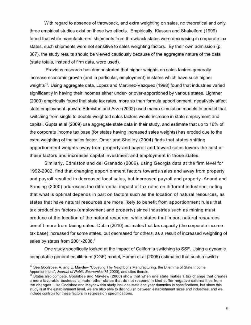
With regard to absence of throwback, and extra weighting on sales, no theoretical and only

three empirical studies exist on these two effects. Empirically, Klassen and Shakelford (1999)

found that while manufacturers’ shipments from throwback states were decreasing in corporate tax

states, such shipments were not sensitive to sales weighting factors. By their own admission (p.

387), the study results should be viewed cautiously because of the aggregate nature of the data

(state totals, instead of firm data, were used).

Previous research has demonstrated that higher weights on sales factors generally

increase economic growth (and in particular, employment) in states which have such higher

weights10. Using aggregate data, Lopez and Martinez-Vazquez (1998) found that industries varied

significantly in having their incomes either under- or over-apportioned by various states. Lightner

(2000) empirically found that state tax rates, more so than formula apportionment, negatively affect

state employment growth. Edmiston and Arze (2002) used macro simulation models to predict that

switching from single to double-weighted sales factors would increase in state employment and

capital. Gupta et al (2009) use aggregate state data in their study, and estimate that up to 16% of

the corporate income tax base (for states having increased sales weights) has eroded due to the

extra weighting of the sales factor. Omer and Shelley (2004) finds that states shifting

apportionment weights away from property and payroll and toward sales lowers the cost of

these factors and increases capital investment and employment in those states.

Similarly, Edmiston and del Granado (2006), using Georgia data at the firm level for

1992-2002, find that changing apportionment factors towards sales and away from property

and payroll resulted in decreased local sales, but increased payroll and property. Anand and

Sansing (2000) addresses the differential impact of tax rules on different industries, noting

that what is optimal depends in part on factors such as the location of natural resources, as

states that have natural resources are more likely to benefit from apportionment rules that

tax production factors (employment and property) since industries such as mining must

produce at the location of the natural resource, while states that import natural resources

benefit more from taxing sales. Dubin (2010) estimates that tax capacity (the corporate income

tax base) increased for some states, but decreased for others, as a result of increased weighting of

sales by states from 2001-2008.11

One study specifically looked at the impact of California switching to SSF. Using a dynamic

computable general equilibrium (CGE) model, Hamm et al (2005) estimated that such a switch 10 See Goolsbee, A. and E. Maydew “Coveting Thy Neighbor’s Manufacturing: the Dilemma of State Income Apportionment”, Journal of Public Economics 75(2000), and cites therein. 11 States also compete. Goolsbee and Maydew (2000) show that when one state makes a tax change that creates a more favorable business climate, other states that do not respond in kind suffer negative externalities from the changes. Like Goolsbee and Maydew this study includes state and year dummies in specifications, but since this study is at the establishment level, we are also able to distinguish between establishment sizes and industries, and we include controls for these factors in regression specifications.

9

would result in increased California employment and tax revenues12. By their own admission,

Hamm et al acknowledged that CGE models are significantly driven by assumptions. Finally,

surveying the literature, the California Legislative Analyst’s Office (LAO) concluded that SSF

adoption would increase California employment when put into effect in 2011.13

In contrast to the above studies, which used largely aggregate data, this study uses an

establishment level econometric estimation methodology. This unique methodology is enabled by

the recent availability of establishment level data, discussed later in the paper. Firm and location

level studies allow more precise estimates of effects (here, the introduction of the SSF) than macro

models, and allow for specific, firm level predictions.

3. MODELING THE SUBSTITUTION EFFECT OF SSF

3.1 General Model

As noted previously, introduction of the SSF has an immediate income effect which causes

an increase (decrease) in investment by instate (out of state) based firms. The substitution effect,

between the SSF and other states in which the firm operates, is more complex. To guide

subsequent empirical tests, we start off with a model. The analysis begins with a simple model of a

firm which operates in a multi-state environment. Although I use a manufacturing example, in

principle, the model can be generalized to any multi-state enterprise where value is added by

various components of the enterprise. To examine the effects of SSF, it is important to also

consider the collateral (and sometimes countervailing) effects, that other aspects of state tax

structures and rates may have. To accomplish this, the model of Williams, Swenson, and Lease

(2001; hereafter WSL) which examined the effects of unitary tax structures (combined reporting)

and tax rates, is extended by examining the effects of SSF. The WSL (2001) model is also

extended to include the effects of sales throwback.

Consistent with WSL (2001), this study models a stylized manufacturing firm with

operations in State 1 and State 2. State 1 can be thought of as where the firm is based or

headquartered. The next few pages review the LSW setup, and then add the effects of SSF. To

add the effects of sales throwback, we enhance the WSL setup by assuming that State 1

operations can also sell directly to customers in nearby State 3 (where the firm has no nexus), and 12 Hamm, W., Alberto, J. and C. Groves, “Apportioning Corporate Income: If California Adopts the Single Factor, What Will be the Economic and Revenue Impact?”. Mimeo, August 2005. 13 Reconsidering the Optional Single Sales Factor: An LAO Report. Sacramento: Legislative Analyst’s Office (May 26, 2010)

10

State 2 operations can also sell to customers in nearby State 4 (where the firm has no nexus). The

firm is considering shifting operations into either State 2 due to the State 2’s switch from double

weighted sales to SSF, or alternatively, into State 1, assuming State 1 switches from double

weighted sales to SSF. Thus, the firm does not face a location choice decision per se. This serves

as a useful starting point to the pure location choice model, discussed later in the paper. To

simplify the analysis, the study assumes that the transactions costs of moving resources to either

State 1 or 2 are equal and exceed return on investment requirements. Thus location costs can be

ignored without generality. The firm is a “classic” example of a unitary business, in that its

multistate operations are functionally dependent on each other, with its headquarters in one state,

and operations in another state; and it clearly has taxable “nexus” (or business connection) in each

of the two states with facilities (States 1 and 2). The model is shown graphically in Figure 3.

The manufacturing process begins at the firm's headquarters in State 1, and the firm

maintains production facilities in State 1 as well. The firm completes production and services

customers in a regional market from the local facility. The firm also completes production in State

2, where output is also sold on a regional basis14. The study models the manufacturing process as

potentially divisible at any stage. That is, at any point in the manufacturing process, the firm could

ship the intermediate (or partially completed) product from the manufacturing center at the

headquarters to the local facilities for completion and sale. The firm incurs a shipping charge for

sending the product from the headquarters to the local facility in State 2 based on the number of

units shipped. The study assumes that the local facility that completes the product and sells to

customers from State 1 is adjacent to the headquarters, and thus no shipping charge is incurred on

those units. The quantities sold to customers from States 1 and 2 are denoted, respectively, as Q1

and Q2.

As management's objective is to maximize the firm's pretax profit, the study initially ignores

state income taxes. Based on the firm's revenue function and the costs it faces, management

chooses the level of capital (K) and labor (L) to employ at each of the firm's three facilities (the

manufacturing center and the local facilities in each state) so as to maximize the excess of revenue

over cost. In making these decisions, management is constrained by exogenously determined

production functions. Management must also choose the point in the manufacturing process at

which production will shift from headquarters to the local production facilities (the degree of

centralization). Denote this as the choice of φ the fraction of the manufacturing process performed

at the headquarters, with (1-φ ) being the percentage performed at the local production facilities,

14 In LSW, production is sold only to customers in the same state. Here, we allow each manufacturing unit to sell production to other nearby states.

11

which is between zero and one. More formally, management chooses Ki, Li, and φ (Є {m, 1, 2}15)

so as to

),,(),(max 2121 QQCQQR −=π (1a)

subject to the production functions for the manufacturing facilities.

Assume the firm operates in an imperfectly competitive market and faces a downward-

sloping demand curve in each state. Specifically, assume the inverse demand function is

,jj bQaP −= where j Є {1, 2}. This leads to the firm's revenue function:

( ) ( )2222

211121 ),( bQQabQQaQQR −+−= . (1b)

Assume the cost of production consists of the rental rate (or, in the alternative, the rate of

return) on capital (r), the wage rate paid for labor (w), and the cost (s) of shipping a unit from the

manufacturing center to the local production facilities in State 2. Assuming a single rental rate on

capital for all facilities, however, allows wage rates to differ between the states. Formally, model

the cost of production as:

( ) ( ) ( ) 2222111121 ),( sQrKLwrKLwrKLwQQC mm ++++++= . (1c)

Assume that production follows a generalized Cobb-Douglas production function where Yi =

LiαKi β with i Є {m, 1, 2}, α and β >0 and < 1. For the headquarters, Ym = φ (Q1 + Q2). For the

local production facilities, Yj = Qj(1-φ ) with j Є {1, 2}. Assume that the productivity of capital does

not depend on its location; accordingly, β is the same for all three production facilities. A realistic

setting should allow for differences in labor between workers in different states. For example, the

average skill level is likely to be different as is the average level and quality of education. One way

of viewing this is to assume that workers with the requisite skill and educational levels are available

in each state, but that local differences in the supply and demand for those workers will potentially

result in different prices for their labor.16 The study however, instead reflects these differences in

the wage rates, wi, rather than in α.

15For notational purposes, I use the subscript m to indicate production or factors of production at the firm's manufacturing center, and I use the subscripts 1 and 2 to indicate production or factors of production at the firm's local production facilities in, respectively, states 1 and 2. 16 Another way to view this is to consider the labor variable, L, as reflecting some unit of human productivity rather than some number of worker-hours. That workers in one state may take longer to achieve that unit of human productivity is

12

Combining equations (1a) and (1b) and specifying the production function constraints, the

pretax model is shown symbolically in (2):

( )22122112

2222

111 )()()1( sQKKKrLwLLwbQQabQQaMax mmu −++−−+−−+−−= τπ

subject to:

( ) ,21βαφ mmm KLYQQ ⋅==+

,)1( 1111βαφ KLYQ ⋅==− and

.)1( 2222βαφ KLYQ ⋅==− (2)

When pretax profits are maximized, wr

MPMP

L

K = (with L

K

MPMP =

KL

αβ ). Therefore,

KL

wr

αβ

= ,17 which is

rearranged as

rwLKαβ

= (adding the appropriate subscripts). (3)

To solve this problem, the first step is to substitute (3) into each constraint for (2), and solve

for the respective L in terms of the Q’s, φ, and exogenous variables. This result is then substituted

into (2). The next step is to hold the Q’s constant and solve for φ by differentiating the resultant

equations with respect to the exogenous variables to obtain the first order conditions (FOC).

reflected, ceteris paribus, in a higher effective wage rate, w. The fact that it would take workers in one state longer to achieve this unit of higher productivity could be reflected in a lower nominal wage rate, but other factors may also influence the nominal wage rate, so the effective wage rates may still differ between the states. I believe this model is generalizable in two important respects. First, I believe it is general enough to encompass both the decision of how to employ resources within existing facilities and the decision as to the size and scope of new facilities. The model ignores the transactions costs associated with these decisions, but if the opening of a new facility (or the expansion of an existing facility) is done through renting a building and equipment and hiring local employees, the transactions costs should be relatively low. Secondly, the model can be generalized to the cases of merchandisers and service companies. In both cases, if proximity to customers and clients is necessary or expected, the firm's choice of how big a facility to employ (capital) and how fully to staff it (labor) will affect the firm's effective state income tax rate. This impact on effective state tax rates could influence, for example, a consulting firm's decision whether to open an office in another state on a full- or part-time basis. While the specification of the parameters (e.g., α and β ) are likely to change, the general form of the model should still apply, and the results may be qualitatively similar.

13

The next few sections enhance the basic model by considering the effects of switching to

SSF when the firm faces a variety of unitary/separate accounting and sales throwback situations.

The examples are not meant to be comprehensive, and instead illustrate some general themes.

3.2 SSF State Uses Separate Accounting

Before examining the effects of SSF, it is useful to first examine the effects of non-unitary

taxation (separate accounting) on resource allocation. First, assume that the firm’s out of state

operations are all in separate accounting states.

3.2.1 Firm Separately Incorporates Each Operation, and Operates only In Separate Accounting

States

The simplest case is where the firm separately incorporates all operations. First, note that

non-unitary taxation of a subsidiary with only single-state operations, does not involve the use of

factor apportionment.18 Hence, taxation of the firm is similar to a tax on pure profits, which is non-

distortionary. With multi-state taxation and a transfer price set equal to average unit cost, I can

separate total profits into two pieces, corresponding to the tax code as follows:

).)(1(

and),)(1(

,

222222

22222

11112

11111

21

sQQprKLwbQQa

QprKLwbQQa

t

t

−−−−−−=

−−−−−=

+=

τπ

τπ

πππ

(4)

Note that the manufacturing center costs are included implicitly, since pt(Q1 + Q2) = w1Lm +

rKm. The transfer prices designate how much of the manufacturing center cost is deductible in

each state. Technically, all those costs are deductible in State 1, but the State 1 firm must also

recognize revenue from sales to State 2 of the unfinished product equal to ptQ2.

If the transfer price is treated as fixed, then the two states’ production and sales decisions

can be made independently. In that case, the taxes are proportionate to economic profits. It is a

well-known result in public economics that a tax on pure profits does not distort factor inputs or

sales decisions. Hence, any effect of a non-unitary tax on resource allocation must be due to an

effect on the transfer price itself, which would be second order in nature. Here, differences in tax

18 Technically, factor apportionment may be employed, but since the three factors are 100% because the subsidiary has operations in only one state; it is “as if” factor apportionment is ignored in this case.

14

rates have no effect on labor or capital between the two states. Even if the transfer price is not

fixed, as shown in equations (A1) and (A2) in Appendix 2, differences in tax rates have very little

effect on labor and capital decisions.

The same analysis applies where one state switches to SSF. Assume State 2 switches

from a double weighted sales factor, to SSF. Since 100% of State 2 net income is still taxed in

State 2, the switch to SSF is generally irrelevant and does not affect labor or capital choices. The

same non-effect occurs if it is State 1 which switches to SSF. Moreover, the effect of sales

throwback is irrelevant, since 100% of profits are taxed in each state in any event; see Equations

(A3) through (A5) in Appendix 2.

The overall result is that there is no effect on resource allocation, due to SSF, when the

firm operates solely in separate accounting states, and incorporates each operation.

3.2.2 Firm Does Not Separately Incorporate Out of State Operations

Suppose again that the firm has operations in State 2, but in this case, does not separately

incorporate them. Thus, while both State 1 and State 2 tax the firm, the firm’s operations will be

apportioned between the two states based on their relative three factor formulas.

Before examining the effects of SSF, it is useful to first examine the general effects of tax

structures on production and investment decisions. Here, the profit equation (2) is multiplied by tax

rates, resulting in (where tτ is the firm’s total multistate tax, and assuming initially that a double

weighted sales factor is used):

]2)21(22)1(12

2222

111)[1( sQKKmKrLwLmLwbQQabQQatMax −++−−+−−+−−= τπ

subject to:

,)( 21βαφ mmm KLYQQ ⋅==+

,)1( 1111βαφ KLYQ ⋅==− and

,)1( 2222βαφ KLYQ ⋅==− with

⎟⎟⎟

⎠

⎞

⎜⎜⎜

⎝

⎛

−+−

−⋅+

++

++

++

+= 2

2222

111

21112

21

1

2211

1141

bQQabQQa

bQQa

KKmK

KmK

Lw)Lm(Lw

)Lm(Lwτtτ

15

⎟⎟⎠

⎞⎜⎜⎝

⎛

−+−−

⋅+++

+++

+ 2222

2111

2222

21

2

2211

222 2)(4 bQQabQQa

bQQaKKK

KLwLLw

Lw

mm

τ . (5)

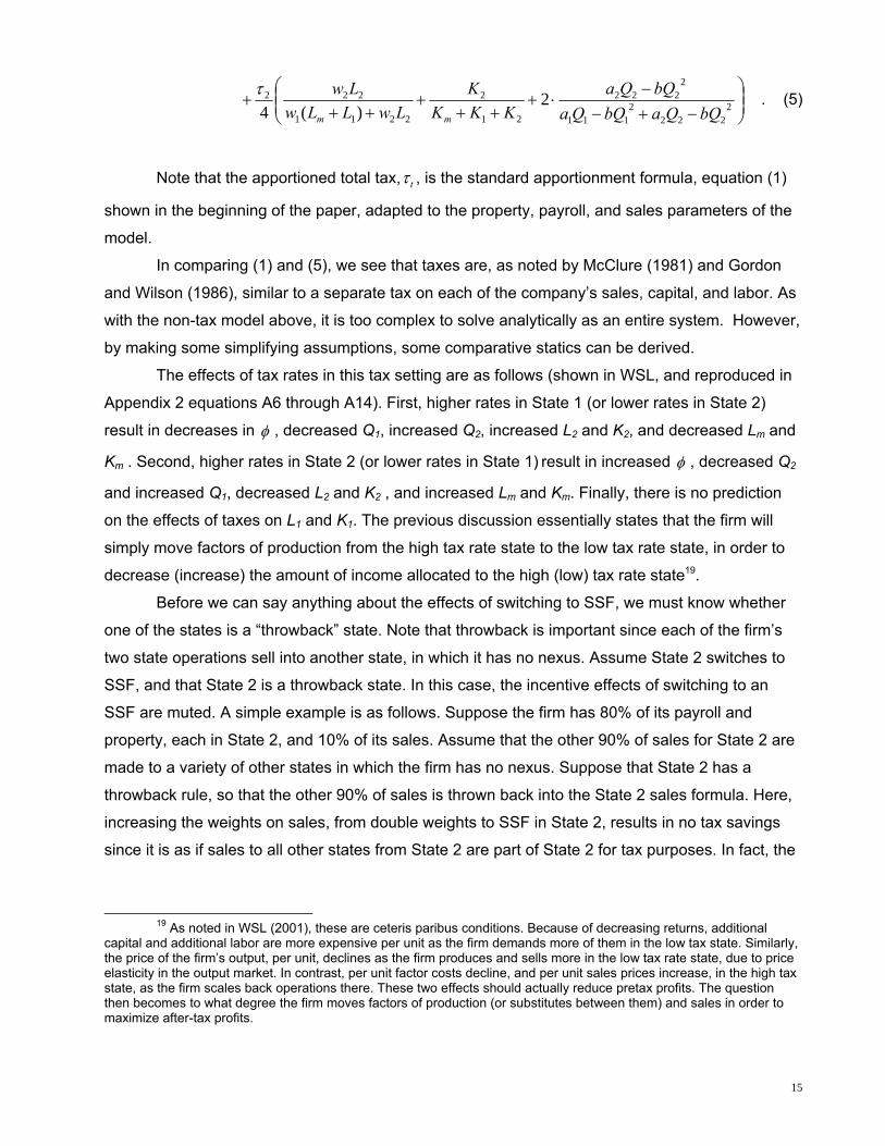
Note that the apportioned total tax, tτ , is the standard apportionment formula, equation (1)

shown in the beginning of the paper, adapted to the property, payroll, and sales parameters of the

model.

In comparing (1) and (5), we see that taxes are, as noted by McClure (1981) and Gordon

and Wilson (1986), similar to a separate tax on each of the company’s sales, capital, and labor. As

with the non-tax model above, it is too complex to solve analytically as an entire system. However,

by making some simplifying assumptions, some comparative statics can be derived.

The effects of tax rates in this tax setting are as follows (shown in WSL, and reproduced in

Appendix 2 equations A6 through A14). First, higher rates in State 1 (or lower rates in State 2)

result in decreases in φ , decreased Q1, increased Q2, increased L2 and K2, and decreased Lm and

Km . Second, higher rates in State 2 (or lower rates in State 1) result in increased φ , decreased Q2

and increased Q1, decreased L2 and K2 , and increased Lm and Km. Finally, there is no prediction

on the effects of taxes on L1 and K1. The previous discussion essentially states that the firm will

simply move factors of production from the high tax rate state to the low tax rate state, in order to

decrease (increase) the amount of income allocated to the high (low) tax rate state19.

Before we can say anything about the effects of switching to SSF, we must know whether

one of the states is a “throwback” state. Note that throwback is important since each of the firm’s

two state operations sell into another state, in which it has no nexus. Assume State 2 switches to

SSF, and that State 2 is a throwback state. In this case, the incentive effects of switching to an

SSF are muted. A simple example is as follows. Suppose the firm has 80% of its payroll and

property, each in State 2, and 10% of its sales. Assume that the other 90% of sales for State 2 are

made to a variety of other states in which the firm has no nexus. Suppose that State 2 has a

throwback rule, so that the other 90% of sales is thrown back into the State 2 sales formula. Here,

increasing the weights on sales, from double weights to SSF in State 2, results in no tax savings

since it is as if sales to all other states from State 2 are part of State 2 for tax purposes. In fact, the

19 As noted in WSL (2001), these are ceteris paribus conditions. Because of decreasing returns, additional

capital and additional labor are more expensive per unit as the firm demands more of them in the low tax state. Similarly, the price of the firm’s output, per unit, declines as the firm produces and sells more in the low tax rate state, due to price elasticity in the output market. In contrast, per unit factor costs decline, and per unit sales prices increase, in the high tax state, as the firm scales back operations there. These two effects should actually reduce pretax profits. The question then becomes to what degree the firm moves factors of production (or substitutes between them) and sales in order to maximize after-tax profits.

16

overall State 2 apportionment would go to 100%. Hence, there is no incentive to move production

from State 1 to State 2.

Suppose instead that State 2 (which switches to SSF), does not have a throwback rule.

Recall that State 2 operations also sell into nearby State 4, where the firm has no production

facilities and no nexus. Θ 2 is the fraction of State 2 production sold to State 2 customers, and 1-

Θ 2 is the proportion sold to State 4 customers. (Similarly, Θ 1 is the fraction of State 1 production

sold to State 1 customers, and 1-Θ 1 is the proportion sold to State 3 customers). Since States 2

and 4 are contiguous, assume that demand functions are similar between the two states. When

there is no sales throwback rule, and sales are double-weighted, the last term in (5) is rewritten as:

( ) ( )( )⎟⎟⎠⎞

⎜⎜⎝

⎛

−Θ−+−Θ+−−

⋅+++

++

+++

= 22221

22221

2111

2111

21

1

2211

111

12

)()(

4 bQQabQQabQQabQQa

KKKKK

LwLLwLLw

m

m

m

mt

ττ

( ) ( )( ) )a5(1

2)(4 2

242222

22222

111

2222

21

2

2211

222⎟⎟⎠

⎞⎜⎜⎝

⎛

−Θ−+−Θ+−−

⋅+++

+++

+QbQabQQabQQa

bQQaKKK

KLwLLw

Lw

mm

τ

With no adjustments to the decision variables, the tax constraints (5a)<(5). Since the

numerator of the sales term in State 2 does not include sales to all other states, there is both an

income and a substitution effect for the firm in State 2. Overall production is shifted to State 2 (Q2

increases). This latter effect actually has a positive externality to State 1: the numerator of the

sales factor decreases resulting in a decrease in tτ . But there is also a negative externality to

State 1; increased production at the main plant increases the transfer price.

To examine the impact of apportionment weights, define the weights for sales, property,

and payroll as Sw, Kw, and Lw, respectively. Since each is defined as a per cent, the sum of the

three weights must equal one. The effects of increased weighting of the sales factor are as follows.

Again assume State 2 switches to SSF. Rewrite (5a) to include apportionment weights for sales,

property, and payroll as follows, assuming throwback:

( ) ( )( ) ⎟⎟⎟⎟⎟

⎠

⎞

⎜⎜⎜⎜⎜

⎝

⎛

−Θ−+−Θ+−

−+−

+++

++

+++

=}

1{

}{})(

)({

223231

22221

2111

23332

2111

1

21

11

2211

111

1

QbQabQQabQQaQbQabQQa

S

KKKKK

KLwLLw

LLwL

w

m

mw

m

mw

t ττ

⎟⎟⎟⎟⎟

⎠

⎞

⎜⎜⎜⎜⎜

⎝

⎛

−+−+−−

+++

+++

+}{

}{})(

{

23333

2222

2111

2222

2

21

22

2211

222

2

QbQabQQabQQabQQaS

KKKKK

LwLLwLwL

w

mw

mw

τ

(6)

17

Assuming no change in resource allocation, the tax constraints (6)<(5a). In fact, (6)<(5). So

in this setting, a switch to SSF results in a shift of resource allocation, due to SSF, into the SSF

state, when the firm operates in a separate accounting state and its out of state operations are not

separately incorporated.

3.2.3 Firm Separately Incorporates Each Operation, and Out of State Operations are Only In A

Unitary (Combined Reporting) State

Before examining the impact of SSF, the general impact of the unitary/separate accounting

structures is examined. Under this specification, and assuming that: State 1 is the non-unitary

state; that the firm separately incorporates its operations in each state20; and that both states use a

double weighted sales factor, (4) is rewritten:

2]2)21(22)1(1

2222

2111)[11(

TaxsQKKmKrLwLmLw

bQQabQQauMax

−−++−−+

−−+−−= τπ

subject to:21

,122122112

2222

1112 ])()()[1( TaxsQKKKrLwLLwbQQabQQaMax π mmu −−++−−+−−+−−= τ

and2)(4

,2222

2111

2222

21

2

2211

2222 ⎟

⎟⎠

⎞⎜⎜⎝

⎛

−+−

−⋅+

+++

++=

bQQabQQabQQa

KKKK

LwLLwLw

mmu

ττ

( ) ( )( ).11112

11111 KKrLLwQpbQQaTax mmt +−+−−−⋅=τ

21

1

QQLwrKp mm

t ++

= . (7)

Here, tp is the transfer price charged by the manufacturing plant at the headquarters for the

intermediate goods transferred to the facilities in State 2. The transfer price is the average unit 21 The previously stated production functions constraints continue to apply but are omitted here so as to concentrate on the income taxes.

18

cost of the manufacturing center. Note that the transfer price is not a decision variable in the

optimization, although it does depend on total sales.

A priori, whether (7) results in a higher tax than in (5), depends on relative values of K, L,

and Q in each state. The amount of potential shifting of resources out of (into) the unitary state is a

matter of degree, limited by the downward slopes of demand in the two states, as well as the

decreasing returns nature of production at each site. As shown in WSL (2001), if tax rates are

higher (lower) in the non-unitary state, this causes a roughly proportionate decrease (increase) in

after-tax profits from that state regardless of production and sales decisions. Hence, we would

expect a minimal shift in resource allocation. The only clear prediction is that if State 1 is the non-

unitary state, then higher (lower) levels in its tax rate will have a more favorable (unfavorable)

impact on its sales and production than if State 2 is the non-unitary state.

With regard to throwback, again assume that some State 2 production can be sold in

nearby State 4. Absence of sales throwback in State 2 encourages additional sales being sourced

into State 4. When State 2 is the unitary state, rewrite the tax constraints in (7) as:

( ) ( )( ),

12

)()(

42

232322

22222

111

2111

21

1

2211

11

22

⎟⎟⎟⎟⎟

⎠

⎞

⎜⎜⎜⎜⎜

⎝

⎛

−Θ−+−Θ+−

−⋅

+++

++

+++

=

QbQabQQabQQabQQa

KKKKK

LwLLwLLw

m

m

m

m

uτ

τ

and,)()(( 11112

11111 KKrLLwQpbQQaTax mmt +−+−−−⋅=τ

.21

1

QQLwrKp mm

t ++

= (8)

Again, the absence of throwback encourages the firm to increase Q2. This increased

production increases K2, L2, and pt. Increased pt results in a negative externality to State 1. State 1

tax actually decreases to the extent that the sales factor denominator increases (due to an overall

increase in Q1 + Q2). State 2 taxes increase, since the numerator of all components of 2uτ

increase faster than the denominators.

Next, assume that State 2, which has no throwback, switches to SSF. Rewrite the

profit equation (4) for State 2 operations as:

19

)].)(1)(1[(

)]()[()1(2

232322

222222

222222

QbQa

sQQprKLwbQQa t

−Θ−−+

−−−−+−Θ−=

τ

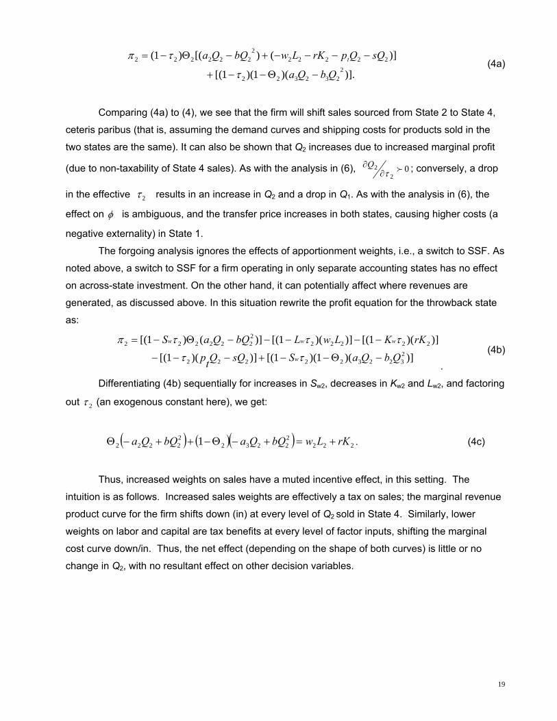
τπ (4a)

Comparing (4a) to (4), we see that the firm will shift sales sourced from State 2 to State 4,

ceteris paribus (that is, assuming the demand curves and shipping costs for products sold in the

two states are the same). It can also be shown that Q2 increases due to increased marginal profit

(due to non-taxability of State 4 sales). As with the analysis in (6), 02

2 fτ∂∂Q ; conversely, a drop

in the effective 2τ results in an increase in Q2 and a drop in Q1. As with the analysis in (6), the

effect on φ is ambiguous, and the transfer price increases in both states, causing higher costs (a

negative externality) in State 1.

The forgoing analysis ignores the effects of apportionment weights, i.e., a switch to SSF. As

noted above, a switch to SSF for a firm operating in only separate accounting states has no effect

on across-state investment. On the other hand, it can potentially affect where revenues are

generated, as discussed above. In this situation rewrite the profit equation for the throwback state

as:

)])(1)(1[()])(1[(

)])(1[()])(1[()]()1[(2322322222

222222222222

QbQaSsQQtprKKLwLbQQaS

w

www

−Θ−−+−−−

−−−−−Θ−=

ττ

τττπ

. (4b)

Differentiating (4b) sequentially for increases in Sw2, decreases in Kw2 and Lw2, and factoring

out 2τ (an exogenous constant here), we get:

( ) ( )( ) 22222232

22222 1 rKLwbQQabQQa +=+−Θ−++−Θ . (4c)

Thus, increased weights on sales have a muted incentive effect, in this setting. The

intuition is as follows. Increased sales weights are effectively a tax on sales; the marginal revenue

product curve for the firm shifts down (in) at every level of Q2 sold in State 4. Similarly, lower

weights on labor and capital are tax benefits at every level of factor inputs, shifting the marginal

cost curve down/in. Thus, the net effect (depending on the shape of both curves) is little or no

change in Q2, with no resultant effect on other decision variables.

20

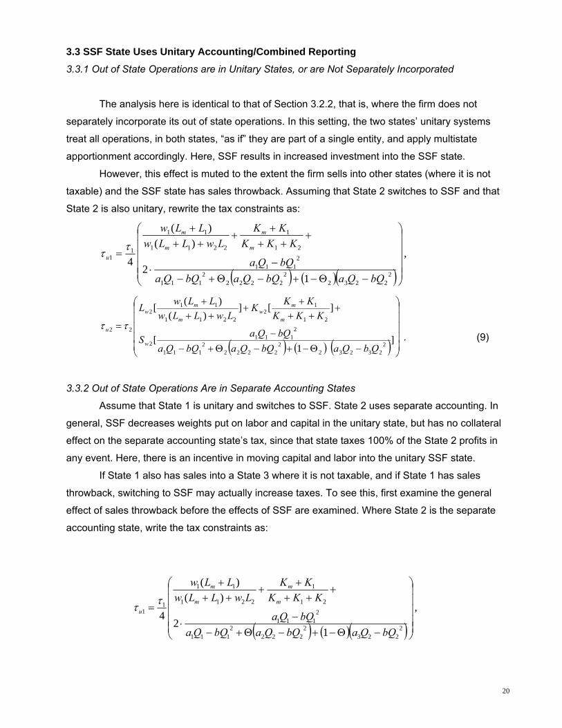
3.3 SSF State Uses Unitary Accounting/Combined Reporting 3.3.1 Out of State Operations are in Unitary States, or are Not Separately Incorporated

The analysis here is identical to that of Section 3.2.2, that is, where the firm does not

separately incorporate its out of state operations. In this setting, the two states’ unitary systems

treat all operations, in both states, “as if” they are part of a single entity, and apply multistate

apportionment accordingly. Here, SSF results in increased investment into the SSF state.

However, this effect is muted to the extent the firm sells into other states (where it is not

taxable) and the SSF state has sales throwback. Assuming that State 2 switches to SSF and that

State 2 is also unitary, rewrite the tax constraints as:

( ) ( )( ),

12

)()(

42

22322

22222

111

2111

21

1

2211

11

11

⎟⎟⎟⎟⎟

⎠

⎞

⎜⎜⎜⎜⎜

⎝

⎛

−Θ−+−Θ+−−

⋅

+++

++

+++

=

bQQabQQabQQabQQa

KKKKK

LwLLwLLw

m

m

m

m

uττ

( ) ( ) ( ) ⎟⎟⎟⎟⎟

⎠

⎞

⎜⎜⎜⎜⎜

⎝

⎛

−Θ−+−Θ+−−

+++

++

+++

=]

1[

][])(

)([

223232

22222

2111

2111

2

21

12

2211

112

22

QbQabQQabQQabQQaS

KKKKKK

LwLLwLLwL

w

m

mw

m

mw

u ττ . (9)

3.3.2 Out of State Operations Are in Separate Accounting States

Assume that State 1 is unitary and switches to SSF. State 2 uses separate accounting. In

general, SSF decreases weights put on labor and capital in the unitary state, but has no collateral

effect on the separate accounting state’s tax, since that state taxes 100% of the State 2 profits in

any event. Here, there is an incentive in moving capital and labor into the unitary SSF state.

If State 1 also has sales into a State 3 where it is not taxable, and if State 1 has sales

throwback, switching to SSF may actually increase taxes. To see this, first examine the general

effect of sales throwback before the effects of SSF are examined. Where State 2 is the separate

accounting state, write the tax constraints as:

( ) ( )( ),

12

)()(

42

2232

2222

111

2111

21

1

2211

11

11

⎟⎟⎟⎟⎟

⎠

⎞

⎜⎜⎜⎜⎜

⎝

⎛

−Θ−+−Θ+−−

⋅

+++

++

+++

=

bQQabQQabQQabQQa

KKKKK

LwLLwLLw

m

m

m

m

uττ

21

and,)( 222222

22222 sQrKLwQpbQQaTax t −−−−−⋅= τ

21

1

QQLwrKp mm

t ++

= . (10)

The additional State 3 sales of Q1 cause two externalities in State 2. Because of concave

production, the increase in Q3 results in a higher transfer price from the primary manufacturer for

both states. Taxes actually increase in State 1 since the denominator of all terms in 1uτ decrease

due to decreases in L2, K2, and Q2.

Next, consider the effects of State 1 switching to SSF. Rewrite the State 1 tax constraints

as:

( ) ( )( ) ⎟⎟⎟⎟⎟

⎠

⎞

⎜⎜⎜⎜⎜

⎝

⎛

−Θ−+−Θ+−−+−

+++

++

+++

=}

1{

}{})(

)({

223231

22221

2111

23332

2111

1

21

11

2211

111

11

QbQabQQabQQaQbQabQQaS

KKKKKK

LwLLwLLwL

w

m

mw

m

mw

u ττ (11)

As with previous analysis, the switch to SSF in such a setting (the home state) is clearly tax

reducing in State 1. The analysis is more complex if State 2 switches to SSF. Since State 2 has

separate accounting, rewrite State 2 tax constraints as:

)],)()()([ 22222222

222222 sQrKKLwLQpbQQaSTax wwtw −−−−−⋅= τ (12a)

if no throwback, and

)],)()()3([ 22222222

332

222222 sQrKKLwLQpbQQabQQaSTax wwtw −−−−−+−⋅= τ (12b) with sales throwback.

It is intuitive that 0/ 22 >∂∂ wSQ because the absence of taxes on State 4 sales increases the

marginal revenue product of State 4, so K2, L2, and Pt all increase beyond the levels caused by the

absence of throwback. A negative externality to State 1 results from the increased transfer price. A

positive externality for State 1 results from the increase in the denominator of 2uτ .

22

3.4 SUMMARY OF SUBSTITUTION EFFECTS The model presented in Sections 3.1 through 3.3 show that the substitution effect is quite

complex. The substitution effect depends on the tax structure in the SSF state versus the other

states in which the firm operates (combined reporting versus separate reporting), and throwback

rules used in the states where the firm operates. The model gives a reasonable first approximation

by simplifying the world by assuming the firm operates in only one other state besides the SSF

state, when in reality, the non-SSF state is likely to be a number of states having a variety of

reporting and throwback rules. Empirically, we see that the data only allow us to know with

certainty the firm’s SSF operations by state, although we can be sure if the firm has multistate

operations, if it is primarily based in the SSF state or primarily based elsewhere, etc. However, we

do have the clear-cut predictions that if the SSF state has unitary/combined reporting, the

substitution effect is generally positive, and that sales throwback in the SSF state generally has a

negative substitution effect.

3.5 FIRM CAN CHOOSE BETWEEN TWO STATES

The previous analyses assumed that a given firm faced a choice of changing existing

operations in a state(s) in which it already operates. The model is robust to situations where a

single facility is expanded, or new facilities are added to augment existing facilities (assuming

some interdependence of operations in the same state). Where the firm faces a choice of locating

a new facility in a new state, under very restrictive conditions, the firm’s location choice is a simple

corner solution; holding all other effects constant, the firm would locate in the state having the most

generous tax benefits. Of course, tax costs of one type may offset tax benefits of another type, in

any one state. Holding all such factors constant, the firm would chose to locate in an SSF state

(versus a non-SSF state) if, as noted in Section 2.2, its out of state sales intensity is high relative to

its plant (labor plus capital) intensity. At one extreme, if at the new facility the firm intended to serve

only that state’s customers, sales weighting factors would have only limited effect. At the other

extreme, if the firm locates a large facility which serves a large number of other states, an SSF

state would be beneficial. Such benefits are increased, if the state uses unitary accounting

(combined reporting), and decreased if the state has sales throwback.

23

4. EMPIRICAL TESTS

To test the above predictions about the effects of single sales factors, we utilize “natural

experiments” which occurred recently in five states: Georgia, Louisiana, New York, Oregon, and

Wisconsin. Georgia switched from double-weighted sales factors to SSF with a three year phase-

in, with sales weightings of 80% in 2006, 90% in 2007, and 100% by 200822. Louisiana completely

switched to SSF after 200523. New York switched to 80% sales weighting in 2006, and 100% in

2007 and later years24. Oregon completely switched to SSF after July 1, 200525. Wisconsin

switched to 60% sales weighting in 2006, 80% in 2007, and 100% in 2008 and later years26.

4.1 Econometric Approach In this section, the econometric approach and the unit of analysis for measuring the labor

and sales impact, from a state switching to a single sales factors (SSF) designation in 2006, is

described. Only firms with multi-state operations are affected, and are denoted as SSFA. The

paper examines the impact of the SSF at the establishment level, for every location of the firm. The

advantages of using establishment-level locations, instead of aggregate firm operations, are:

1. comparisons to non- SSF firms are less influenced by size effects (SSF firms tend to be larger

than non-SSF firms, but this is less severe when individual establishment locations are examined);

and 2. more powerful tests are enabled with a larger number of observations. The analysis

considers the effects of trends by using a differences in differences (DID) estimation method27. In

contrast to a within-subjects estimate of the treatment effect (that measures the difference in an

outcome after and before treatment), or a between-subjects estimate of the treatment effect (that

measures the difference in an outcome between the treatment and control groups), the DID

estimator represents the difference between the pre-post, within-subjects differences of the

treatment and control groups.

The basic premise of DID is to examine the effect of some sort of treatment by comparing

the treatment group after treatment, both to the treatment group before treatment, and to some

other control group. While it might be tempting to consider simply looking at the treatment group

before and after treatment, to try to deduce the effect of the treatment, a number of other factors

might be going on at the exact same time as the treatment. DID uses a control group to control for

the effects of other changes at the same time, assuming that these other changes were similar 22 O.C.G.A Sec. 48-7-31 23 Sec. 47:287.95(F)(2)(a) 24 Sec. 210 (3)(a)(10) Tax Law 25 Sec. 314.650 ORD 26 Sec. 71.25(6) Wisc. Stats. 27 For examples of the DID method, see Card and Kreuger (1994); and also Ham, Swenson, Imrohoroglu, and H. Song (2011)

24

between the treatment and control groups.

Because only some of the firms in a state have multi-state operations and are affected by

the SSF, the control group of firms was designated which are single-state only, and are not

affected by the SSF (denoted as SSFN). With DID estimation methods, we can use this latter

group of firms as a control. Unfortunately, using matched pairs of SSFA and SSFN firms is

problematic; because SSFA and SSFN firms may vary on a number of attributes, any resultant

matching appears difficult. Instead, these two groups of firms are pooled in state-by-state

regressions. Because the analysis did not have access to a national firm dataset (such a dataset is

prohibitively costly28), standard errors may be inflated, which would bias against finding results.

Later, we shall see that despite such a conservative approach, the data reveals the significant

impacts of SSF adoption. The DID estimation method is discussed next.

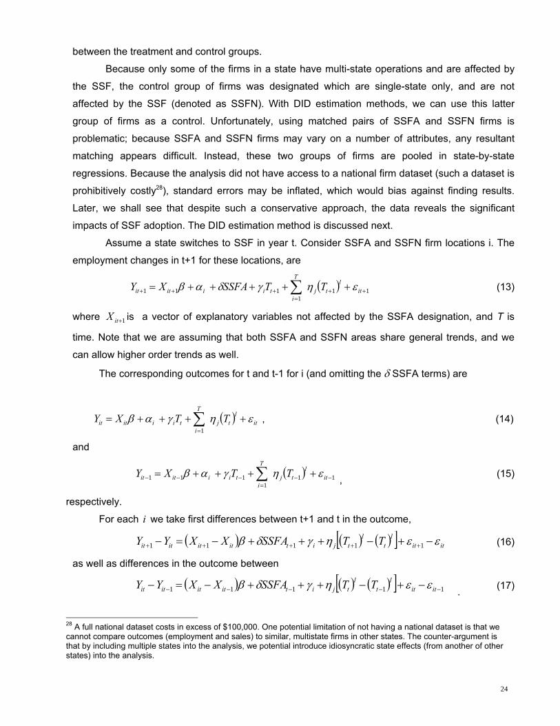
Assume a state switches to SSF in year t. Consider SSFA and SSFN firm locations i. The

employment changes in t+1 for these locations, are

( ) 111

111 ++=

+++ +++++= ∑ itl

tj

T

itiiitit TTSSFAXY εηγδαβ (13)

where 1+itX is a vector of explanatory variables not affected by the SSFA designation, and T is

time. Note that we are assuming that both SSFA and SSFN areas share general trends, and we

can allow higher order trends as well.

The corresponding outcomes for t and t-1 for i (and omitting the δ SSFA terms) are

( ) itl

tj

T

itiiitit TTXY εηγαβ ++++= ∑

=1 , (14)

and

( ) 111

111 −−=

−−− ++++= ∑ itl

tj

T

itiiitit TTXY εηγαβ , (15)

respectively.

For each i we take first differences between t+1 and t in the outcome,

( ) ( ) ( )[ ] ititl

tl

tjititititit TTSSFAXXYY εεηγδβ −+−+++−=− +++++ 11111 (16)

as well as differences in the outcome between

( ) ( ) ( )[ ] 11111 −−−−− −+−+++−=− ititl

tl

tjititititit TTSSFAXXYY εεηγδβ . (17)

28 A full national dataset costs in excess of $100,000. One potential limitation of not having a national dataset is that we cannot compare outcomes (employment and sales) to similar, multistate firms in other states. The counter-argument is that by including multiple states into the analysis, we potential introduce idiosyncratic state effects (from another of other states) into the analysis.

25

Double differencing by subtracting (17) from (16) for each i yields

( ) ( )[ ]( )[ ]( ) ( ) ( )[ ] ( ) .22

2

1111

111

11

−+−+

+−+

−+

+−++−+

++−=−−−=

itititl

tl

tl

tj

tititit

ititititi

TTT

SSFAXXXYYYYZ

εεεη

δβ

(18)

A research design questions is: what set of SSFN firms do we use as a control group? In the

following analyses we use two such control groups: all other firms in the SSF state; and all other

firms in the state which are multi-location (but have no multistate operations). This latter control

group may bear more similarity to SSF firms, but the trade-off is that there are fewer of them, and

this reduces the power of our tests.

As a validation of the DID approach, we also use a simple levels change model, which looks

at levels of employment over time in both the SSF and SSFN firms, as a function of the prior year’s

employment, as follows:

Yit-1= Xitβ + αi + δ SSFAt + ζtYR t + εit , (19) where YR are year indicator variables. SSFA is set to 1 if the firm is subject to SSF (and zero

otherwise), and the year is set to 1 after SSF enactment (and zero otherwise).

As a final specification test, we run the above models state-by-state, and also with all five

states pooled.

4.2 Data

The 2008 National Establishment Time-Series (NETS) Database is a unique, firm (and

location) specific database derived from the Dun & Bradstreet data, the latter of which is used

commercially. This data set became available to academics in 2007. The 2008 NETS Database

includes an annual time-series of information on over 36.5 million U.S. establishments from

January 1990 to January 2008. Since the current Database is based on 19 "snapshots" taken

every January of the Dun and Bradstreet data, it reflects the economic activity of the previous

years (1989-2008). The Database is as close to an annual census of American business as

exists. Among other establishment level items, this database reports sales, employment, industry

(at 8 digit levels), exact location, and affiliation with other establishments (parents,

subsidiaries, number of other establishments within the same legal entity).

A number of academic papers have begun to use this database.29 It is important to note

that each observation is a single location, i.e., observations are not aggregated to the entity level.

Such disaggregation allows for very powerful tests by increasing the number of observation, and 29 For example, N. Wallace (U.C. Berkeley) has a paper on "Agglomeration Economies and the HiTech Computer Sector": http://repositories.cdlib.org/iber/fcreue/fcwp/292 and “The Role of Job Creation and Job Destruction Dynamics” in Glaeser & Quigley, Housing Markets and the Economy (2009).

26

avoiding any “masking” of effects, which might occur with aggregate data, if firms simply move

employees from one location to another.

Recall from earlier in the paper that we predict potentially different results for in-state based

firms, versus out of state firms. Accordingly, we identify each location as belonging to either set30

for the SSFA firms. Although the primary variable of interest is employment, the NETS data also

reports sales, so we examine this variable as a collateral measure of business expansion.

4.4 Results 4.4.1 Georgia

Descriptive statistics for Georgia are shown in Table 1 for 2002 through 2008. There are

1,182,732 observations (recall that observations are individual locations). However, only 298,675

have complete sets of data; on average (sales and employment from 2002 through 2008), 45,668

of the complete observations belong to the SSFA group.

The overall state sample (both SSFA and SSFN firms) shows a mean sales decline of 21%

for 2006-2008 (post SSF). Throughout the analysis, it is important to note that the recession began

in late 2007, and continued through 2008. Accordingly, we would expect downward trends in

employment during this period. SSFA firms show sales changes in the same time period of +3.7%.

Thus, average SSFA locations showed higher sales growth after SSF enactment. For employment,

the Table shows that for all firms, employment declined 18.3%, post-SSF adoption, while SSFA

firms exhibit a 4.1% employment growth, after Georgia became an SSF state.

Regression results for Georgia are reported in Table 6. Regression results for sales are

shown in the left side of the Table. Model 1 uses all non SSF firms as the control (omitted) group;

Model 2 uses only multi-location, single state firms as a control group. Both models use a

difference in differences (DID) design. Model 3 uses all non-SSF firms as controls, and instead of a

DID specification, simply models annual sales as a lagged function of previous years’ sales.

Consistent with expectations, all three models show that locally-based multi-state firms expanded

operations (in terms of local sales, significant at .001 for all models) after SSF enactment. In

contrast, all models show that out of state-based firms scaled back their operations (in terms of

locally based sales), indicating that the negative income effect of the SSF dominated the positive

substitution effect.

Regression results for employment, using the same three model specifications, are shown in

the right side of Table 6. Consistent with expectations, locally based firms increased employment

30 In the NETS dataset, a multi-state firm is out of state if its DUNSHQ state is different form the state in which in which the location operates. An instate, multi-state firm has a DUNSHQ in the same state.

27

(for all models, at a .001 level of significance) after enactment of SSF. Two of the three models

show that out of state-based firms decreased their local employment, indicating that the negative

income effect dominated the positive substitution effect.

4.4.2.Louisiana Descriptive statistics for Louisiana are shown in Table 2 for 2002 through 2008. Note that

major hurricanes hit Louisiana in late 2005, but their aftermaths have unclear differential effects on

SSF versus non-SSF firms, a priori. There are 532,386 observations (recall that observations are

individual locations). However, only 248,526 have complete sets of data, and on average (sales

and employment from 2002 through 2008), 40,511 of these belong to the SSFA group.

The overall state sample (both SSFA and SSFN firms) shows a mean sales increase of 13%

from 2006 to 2008 (post SSF). SSFA firms show sales growth in the same time period of 3.7%. For

employment, the Table shows that for all firms, employment declined 17% post-SSF adoption,

while SSFA firms exhibit a 7% employment growth after Louisiana became an SSF state.

Regression results for Louisiana are reported in Table 7. Regression results for sales are

shown in the left of the Table. Model 1 uses all non SSF firms as the control (omitted) group; model

2 uses only multi-location, single state firms as a control group. Both models use a difference in

differences (DID) design. Model 3 uses all non-SSF firms as controls, and instead of a DID

specification, simply models annual sales as a lagged function of previous years’ sales. Consistent

with expectations, all three models show that locally-based multi-state firms expanded operations

(in terms of local sales, significant at .001 for all models) after SSF enactment. In contrast, all

models show that out of state based firms scaled back their operations (in terms of locally based

sales), indicating that the negative income effect of the SSF, dominated the positive substitution

effect.



(for all models, at a .001 level of significance) after enactment of SSF. For out of state based firms,

there is not much change in employment (although one of the three models shows a significant

employment decline), indicating that the negative income effect may have offset the positive


4.4.3 New York

Descriptive statistics for New York are shown in Table 3 for 2002 through 2008. There are

2,433,791 observations (recall that observations are individual locations). However, only 1,098,706

28


of these observations with complete data belong to the SSFA group.

The overall state sample (both SSFA and SSFN firms) shows a 22.7% sales decline for

2006-2008 (post SSF). As noted previously, it is important to note that the recession began in late

2007, and continued through 2008. SSFA firms show sales changes in the same time period of

+7.1%. Thus, average SSFA locations showed higher sales growth after SSF enactment. For

employment, the Table shows that for all firms, sales declined 12.5% post-SSF adoption, while

SSFA firms show sales growth of 3.1% for post SSF adoption.

Regression results for New York are reported in Table 8. Regression results for sales are



differences in differences (DID) design. Model 3 uses all non-SSF firms as controls, and instead of

a DID specification, simply models annual sales as a lagged function of previous years’ sales.



contrast, all models show that out of state based firms scaled back their operations (in terms of

locally based sales), indicating that the negative income effect of the SSF, dominated the positive





show that out of state-based firms decreased their local employment, indicating the negative

income effect, dominated the positive substitution effect.

4.4.4 Oregon

Descriptive statistics for Oregon are shown in Table 4 for 2002 through 2008. There are

538,231 observations (recall that observations are individual locations). However, only 235,198

have complete sets of observations; on average (sales and employment from 2002 through 2008),

31,841 of these observations with complete data belong to the SSFA group.

The overall state sample (both SSFA and SSFN firms) shows mean sales declines of 3.7%

for 2006-2008 (post SSF). As noted previously, it is important to note that the recession began in

late 2007, and continued through 2008. SSFA firms show sales increases in the same time period

of 12.5%. Thus, average SSFA locations showed higher sales growth after SSF enactment. For

employment, the Table shows that for all firms, employment declined 8.5% post-SSF adoption,

29

while SSFA firms show 6.6% increases in employment post-SSF adoption.

Regression results for Oregon are reported in Table 8. Regression results for sales are




DID specification; simply models annual sales as a lagged function of previous years’ sales.



contrast, all models show that out of state-based firms scaled back their operations (in terms of




the right side of Table 8. Consistent with expectations, locally-based firms increased employment


show that out of state-based firms decreased their local employment, indicating the negative

income effect, dominated the positive substitution effect.

4.4.5 Wisconsin

Descriptive statistics for Wisconsin are shown in Table 5 for 2002 through 2008. There are

602,327 observations (recall that observations are individual locations). However, only 298,675


of these observations with complete data belong to the SSFA group.

The overall state sample (both SSFA and SSFN firms) shows a mean sales decline of 8.1%

for 2006-2008 (post SSF). As noted previously, it is important to note that the recession began in

late 2007, and continued through 2008. SSFA firms show sales changes in the same time period of

+9.2%. Thus, average SSFA locations showed higher sales growth after SSF enactment. For

employment, Table 5 shows that for all firms, employment declined 12.2% post-SSF adoption,

while SSFA firms exhibit a 4.3 % employment growth after Georgia became an SSF state.

Regression results for Wisconsin are reported in Table 10. Regression results for sales are




DID specification, simply models annual sales as a lagged function of previous years’ sales.


30


contrast, all models show that out of state based firms scaled back their operations (in terms of


substation effect.

Regressions results for employment, using the same three model specifications, are shown

in the right side of Table 6. Consistent with expectations, locally-based firms increased

employment (for all models, at a .001 level of significance) after enactment of SSF. Two of the

three models show that out of state-based firms did not significantly change their local

employment, indicating the negative income effect may have offset the positive substitution effect.

4.4.6 All States Combined The advantage of analyzing each of the five SSF states individually is that it allows for

differing state trends. However, the effects of individual state policies, such as unitary versus

separate accounting, and sales throwback, cannot be directly tested since the same policy applies

to all firms in that state. If we pool observations from all states, we can test the mitigating effects of

such state policies on investment after SSF, noting that noise may be introduced into the sample

due to differing economic trends across the states.

For this analysis, we add two dummy variables if the state follows unitary

accounting/combined reporting (one for locally-based multistate firms, and one for out of state

based multistate firms, and each set to zero for all other firms). Recall from the theory, that if the

SSF state is also unitary, there is an additional tax advantage to investment in the state after SSF

enactment (a positive substitution effect), which should be an increasing function of investment in

that state (i.e., more significant for locally-based firms). Here, only Oregon follows unitary

(combined) reporting.31

We also add two dummy variables if the state has sales throwback (one for locally-based

multistate firms, and one for out of state based multistate firms, and each set to zero for all other

firms). Recall from the theory, that if the SSF state has sales throwback, there is a decreased tax

advantage to investment in the state after SSF enactment (a negative substitution effect), which

should be an increasing function of investment in that state (i.e., more significant for locally-based

firms). Here, only Oregon and Wisconsin have sales throwback.32

Regression results are reported in Table 11. Regression results for sales are shown in the

31 Note that after 2008, Wisconsin switched to combined reporting, and New York began requiring combined reporting for firms with substantial inter-company transactions 32 For each dummy variable (unitary and throwback), the omitted state (to avoid colinearity) is Georgia, which follows separate accounting, and does not have throwback.

31

left side of the Table. Model 1 uses all non SSF firms as the control (omitted) group; Model 2 uses

only multi-location, single state firms as a control group. Both models use a difference in

differences (DID) design. Model 3 uses all non-SSF firms as controls, and instead of a DID

specification; simply models annual sales as a lagged function of previous years’ sales. Consistent

with expectations, all three models show that locally-based multi-state firms expanded operations

(in terms of local sales, significant at .001 for all models) after SSF enactment. In contrast, all

models show that out of state based firms scaled back their operations (in terms of locally based

sales), indicating that the negative income effect of the SSF, dominated the positive substation

effect. Both of these findings are consistent with the by-state regression results.

For throwback, we see that locally-based firms experience reduced sales in throwback

states, after SSF enactment, in all regressions. In contrast, out of state-based firms’ sales are not

significantly affected by SSF in throwback states. Consistent with expectations, out of state-based

firms experience sales growth after SSF enactment in unitary states, but there is very little effect for

out of state-based firms.

Regressions results for employment, using the same three model specifications, are shown

in the right of Table 11. Consistent with expectations, locally based firms increased employment


show that out of state-based firms did not significantly change their local employment, indicating

the negative income effect may have offset the positive substitution effect. For throwback,

consistent with expectations, we see a negative effect for locally-based firms, and relatively little

effect for out of state-based firms. For unitary tax structures, we see that employment increased for

locally-based firms (in two out of the three models) in unitary states, but there was no effect for out

of state-based firms in unitary states.

In summary, the pooled states’ regressions are supportive of predictions. That is, after SSF

enactment: locally-based firms expanded their operations; out of state-based firms did not change

or decreased their operations; states with unitary tax structures (here, Oregon) resulted in

incremental business activity for locally-based firms (but not out of state-based firms); and states

with sales “throwback” (Oregon and Wisconsin) had a dampening effect on locally-based

businesses (but not out of state-based businesses).

Recall from the theory section that there may be some accentuation of policy effects based

on tax rates. While the tax rate effects are relative (rates in the state switching to SSF, versus rates

in all other states where the firm operates) and we can only observe tax rates in the SSF state, we

might nonetheless be able to detect some tax rate effects. Accordingly, variables were multiplied

by average (of 2005-8) top corporate rates for each of the SSF states. Regression results from

these newly-measured variables are reported in Table 12. As can be seen results are not much

32

different from Table 11 results, and F tests show these new models’ fits are about the same as

those shown in Table 11. The apparent lack of incremental explanatory power of tax rates may be

due to the modest differences in tax rates across the 5 states examined, or alternatively, due to the

inability (with the data available) to test for the effects of relative tax rates.

5. CONCLUSION This study examines whether switching to an SSF weighting system for corporate state

income taxation is effective in attracting business to a state. Because a firm’s overall state tax

liability is a function of where its payroll (people), property (factories or facilities) and sales are

located, relative differences in state apportionment rules should result in the firm making such

resource decisions. Results of a firm model find that the firm would make such resource allocation

changes to minimize company-wide state taxes, but only under certain conditions. The theory’s

predictions are then empirically tested using firm/location specific data for five states which

switched from double-weighted sales to SSF in 2006: Georgia, Louisiana, New York, Oregon, and

Wisconsin. Using a difference in differences econometric model which is able to discern firms

which are affected by SSF, the model finds that SSF does in fact increased overall employment in

these states after adoption. However, this net employment increase was comprised of an

employment increase for locally-based firms, and a decrease for out of state-based firms.

The policy implications of this may be important since policy-makers have assumed that

switching to SSF would attract businesses to their states, and/or encourage expansion of already

existing businesses. This study provides results which suggest that the policy-makers are generally

right, but there will also be “winners” (locally-based firms) and losers (out of state based firms). Of

course, such policy implications should be tempered; the use of a general equilibrium model may

be appropriate to examine the total effects on both a state’s economy and its overall tax base.

33

REFERENCES

All-State Tax Guide, 2008. Commerce Clearing House. Anand, B. and R. Sansing. 2000. The weighting game: Formula apportionment as an instrument of public policy. National Tax Journal 53 (2): 183-1999. Bartik, T. 1994. Jobs, productivity, and local economic development: What implications does economic research have for the role of government? National Tax Journal 47 (4): 847-861. Brunori, D. 1997. Principles of tax policy and targeted tax incentives. State Tax Notes (June 9): 111-127. Burstein, M. and A. Rolnick. 1996. Congress should end the economic war among the states. State Tax Notes (June 24): 125-44. Card, D. and A Krueger. 1994. Minimum Wages and Employment: A Case Study of the Fast Food Industry in New Jersey and Pennsylvania. American Economic Review 84 (September): 774-775. Carlton, D. 1983. The location and employment choices of new firms: an econometric model with discrete and continuous endogenous variables. The Review of Economics and Statistics 65 (Aug.): 440-449. Carroll, R. and M. Wasylenko. 1994. Do state business climates still matter? Evidence of a structural change. National Tax Journal 47 (1): 19-37. Coughlin, C., Terza, J., and V. Arromalee.1991. State characteristics and the location of foreign direct investment within the united states. The Review of Economics and Statistics 73 (Nov.): 675-683. Dubin, E. 2010. Changes in state corporate tax apportionment formulas and tax bases. Tax Analysts Feb.22: 563-572. Edmiston, K. 2002. Strategic apportionment of the state corporate income tax. National Tax Journal 55 (2): 239-262. Edmiston, K., and F. Arze. 2002. Firm-level effects of apportionment formula changes. Working paper, Georgia State University, Atlanta, GA. Edmiston, K., and F. del Granado. 2006. Economic effects of apportionment formula change: results from a panel of corporate income tax returns. Public Finance Review 43 (September): 483-504. Fox, W., and L. Luna, 2002. State corporate tax revenue trends: causes and possible solutions. National Tax Journal 55 (3), 491–508. Fox, W., and L. Luna, 2005. Do LLCs explain declining state corporate tax revenues? Public Finance Review 33 (6), 690–720. Fox, W., L Luna, and M. Murray, 2005. How should a subnational corporate income tax on multistate businesses be structured? National Tax Journal 58 (1), 139–159.

34

Goolsbee, A. and E. Maydew. 2000. Coveting thy neighbor’s manufacturing: The dilemma of state income and apportionment. Journal of Public Economics 75 (1): 125-143. Gordon, R., and J. Wilson .1986. An examination of multijurisdictional corporate income taxation under formula apportionment. Econometrica (Nov.): 1357-1373. Gupta. S. and M. Hofmann. 2002. The effect of state income tax apportionment and tax incentives on new capital expenditures. Working paper. Arizona State University. Gupta, S. and L. Mills. 2002. Corporate multistate tax planning: benefits of multiple jurisdictions. Journal of Accounting and Economics (22 No. 1): 117-139. Gupta, S., Moore, J., Gramlich, J., and M. Hoffman. 2009. Empirical evidence on the revenue effects of State corporate income tax policies. National Tax Journal (June): 243. Ham, J., Swenson, C., Imrohoroglu, A., and H. Song. 2011. Government programs can improve local labor markets: evidence form state enterprise zones, Federal empowerment zones, and Federal enterprise communities. Journal of Public Economics. (forthcoming) Helms, L. 1985. The effect of state and local taxes on economic growth: A time series-cross section approach. The Review of Economics and Statistics 67 (4): 574-582. Hofmann, M. A. 2002. The state corporate income tax: a synthesis of recent research. Journal of Accounting Literature (21): 76-119. Klassen, K. and D. Shackelford. 1998. State and provincial corporate tax planning: income shifting and sales apportionment factor management. Journal of Accounting and Economics 25 (3): 385-406. Knight, B. 2001. State capital taxes and the location of investment: Empirical lessons from the tax competition models. Working paper, Federal Reserve Board, Washington, D.C. Lightner, T. 2000. The effect of the formulary apportionment system on state-level economic development and multijurisdictional tax planning.” Journal of the American Taxation Association (Supplement) Lopez, S., and J. Martinez-Vazquez. 1998. State corporate income taxation: an evaluation of the formula apportionment system. National Tax Journal (Supplement): 155-161. Luna, L. and M Murray. 2010. The effects of state tax structures on business organizational form. National Tax Journal (63): 995-1022 McLure, C. 1980. The state corporate income tax: lambs in wolves’ clothing. In Aaron, H. & Boskin, M. (Ed.), The Economics of Taxation. Washington, D.C.: Brookings Institution. McClure, C. 1981. The illusive incidence of the corporate income tax: the state case. Public Finance Quarterly (Oct.): 395-413. Mofidi, A. and J. Stone. 1990. Do state and local taxes affect economic growth? The Review of Economics and Statistics 72 (4): 686-691.

35

Moore, M., Steece, B., and C. Swenson .1987. An economic analysis of the impact of state tax rates and bases on foreign investment in the United States. The Accounting Review (October): 671 – 685. Omer, T. and M. Shelley. 2004. Competitive, political, and economic factors influencing state tax policy changes. Journal of the American Taxation Association (26, supplement):103-126. Swenson, C. (ed.). 2009. Bender’s State Taxation: Principles and Practice. Treatise, LexisNexis. Wasylenko, M. 1997. Taxation and economic development: The state of the economic literature. New England Economic Review (March/April): 37-52. Weiner, J. 1996. Estimates of How the Unitary Tax Affects Business Investment. Paper presented at the Allied Social Science Meetings, San Francisco, California. Wetzler, J. 1995. Should the U.S. adopt formula apportionment? National Tax Journal (Sept): 357-362. Williams, M., Swenson, C., and T. Lease. 2001. Effects of unitary versus non-unitary state income taxes on resource allocation: some analytical and simulation results. Journal of the American Taxation Association 23 (Spring). Wilson, J. 1999. Theories of tax competition. National Tax Journal 52 (June): 269-304.

36

Appendix 1 Table 1a-General33 Factor Apportionment, and Sales Throwback, by State for Time Period Examined (as of 12/31/2008; top statutory corporate income tax rate in parentheses) State (Top Marginal Rate)

Sales, Property, and Payroll Weights:

Sales Throwback

State (Top Marginal Tax Rate)

Sales, Property, and Payroll Weights

Sales Throwback

Missouri

(6.25%) 1/3 each Yes

Alabama (6.5%)

1/3 each Yes Montana (6.75%)

1/3 each Yes

Arizona (6.968%)

.5,.25,.25 No Nebraska (7.81%)

1.0,0,0 No

Arkansas (6.5%)

.5,.25,.25 Yes Nevada N/a-no tax N/a-no tax

California (8.84%)

.5,.25,.25 Yes New Hampshire (8.5%)

.43,.285,.285 Yes

Colorado (4.63%)

1/3 each Yes New Jersey (9%)

.5,.25,.25 No

Connecticut (7.5%)

.5,.25,.25 No New Mexico (7.6%)

1/3 each Yes

Delaware (8.7%)

1/3 each No New York (7.5%)

1.0,0,0 No

Florida (5.5%) .5,.25,.25 No North Carolina (6.9%)

.5,.25,.25 No

Georgia (6%) 1.0,0,0 No North Dakota 1/3 each Yes Hawaii (6.4%) 1/3 each Yes Ohio (6.8%)* .5,.25,.25 No Idaho (7.6%) .5,.25,.25 Yes Oklahoma

(6%) 1/3 each No

Illinois (4.8%) 1.0,0,0 Yes Oregon (6.6%)

1.0,0,0 Yes

Indiana (8.5%) .5,.25,.25 Yes Pennsylvania (9.99%)

.5,.25,.25 No

Iowa (12%) 1.0,0,0 No Rhode Island (9%)

1/3 each No

Kansas (4%) 1/3 each Yes South Carolina (5%)

1/3 each No

Kentucky (7%) .5,.25,.25 No South Dakota N/a-no tax N/a-no tax

Louisiana (8%) 1.0,0,0 No Tennessee (6.5%)

.5,.25,.25 No

Maine (8.93%) .5,.25,.25 Yes Texas*(4.5%) 1.0,0,0 Maryland (7%) .5,.25,.25 No Utah (5%) 1/3 each Yes Massachusetts (9.5%)

1.0,0,0 Yes Vermont (8.9%)

1/3 each Yes

33 Note that these formulas are general; certain industries may elect (or are required) to use different formulas

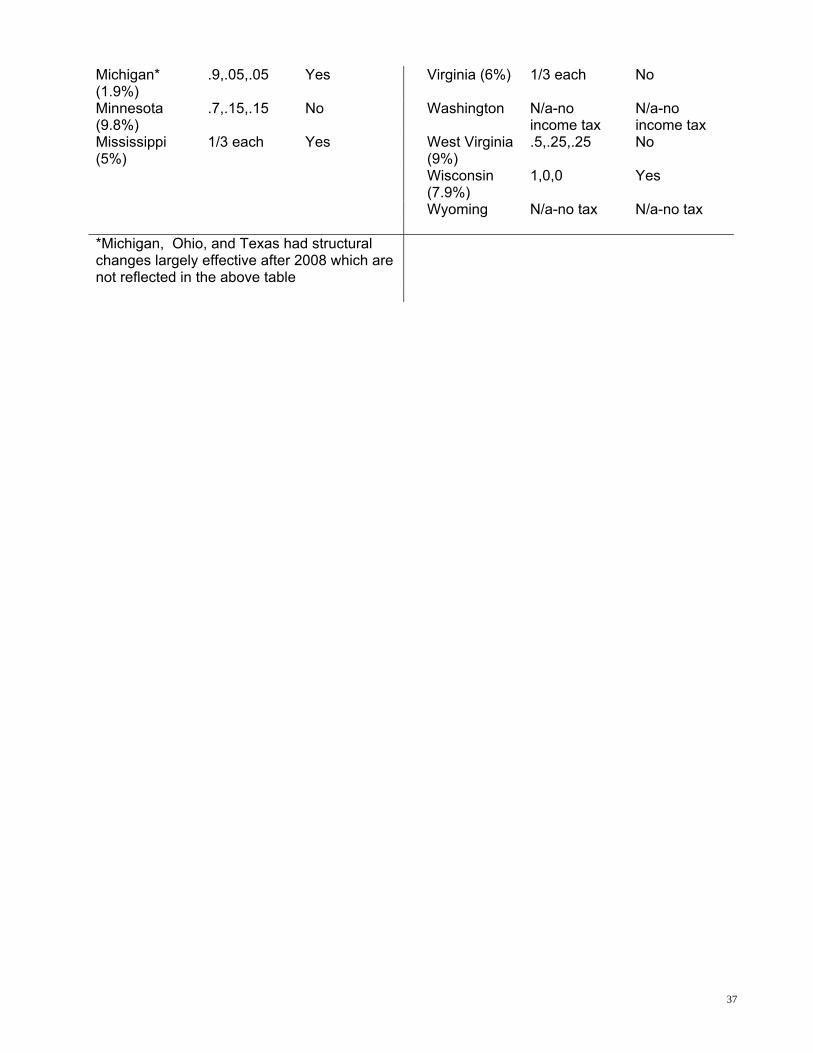
37

Michigan* (1.9%)

.9,.05,.05 Yes Virginia (6%) 1/3 each No

Minnesota (9.8%)

.7,.15,.15 No Washington N/a-no income tax

N/a-no income tax

Mississippi (5%)

1/3 each Yes West Virginia (9%)

.5,.25,.25 No

Wisconsin (7.9%)

1,0,0 Yes

Wyoming N/a-no tax N/a-no tax *Michigan, Ohio, and Texas had structural changes largely effective after 2008 which are not reflected in the above table

38

` Appendix 1 Table 1b-Updated Factor Apportionments (As of 2010) State Sales,

Property, and Payroll Weights:

State Sales, Property, and Payroll Weights

Missouri 1/3 each34 Alabama 1/3 each Montana 1/3 each Arizona .5,.25,.25 Nebraska 1.0,0,0 Arkansas .5,.25,.25 Nevada N/a-no tax California .5,.25,.25 New

Hampshire .43,.285,.285

Colorado 1/3 each35 New Jersey .5,.25,.25 Connecticut .5,.25,.2536 New Mexico 1/3 each Delaware 1/3 each New York 1.0,0,0 Florida .5,.25,.25 North

Carolina .5,.25,.25

Georgia 1.0,0,0 North Dakota 1/3 each Hawaii 1/3 each Ohio 1.0,0,037 Idaho .5,.25,.25 Oklahoma 1/3 each Illinois 1.0,0,0 Oregon 1.0,0,0 Indiana .5,.25,.2538 Pennsylvania .5,.25,.25 Iowa 1.0,0,0 Rhode Island 1/3 each Kansas 1/3 each39 South

Carolina 1/3 each40

Kentucky .5,.25,.25 South Dakota N/a-no tax

Louisiana 1.0,0,0 Tennessee .5,.25,.25 Maine 1.0,0,0 Texas 1.0,0,0 Maryland .5,.25,.2541 Utah 1/3 each Massachusetts 1.0,0,0 Vermont 1/3 each Michigan .9,.05,.0542 Virginia .5,.25,.25 Minnesota 1.0,0,0 Washington N/a-no

income tax Mississippi 1.0,0,0 West Virginia .5,.25,.25 Wisconsin 1,0,0 Wyoming N/a-no tax See also notes in text about SSF restrictions to certain industries, for certain states.

34 SSF is elective 35 Starting in on or after January 1, 2009, multistate corporations must use SSF 36 Financial service companies, broadcasters, and manufacturers must use SSF 37 Under commercial activity tax 38 SSF is being phased in and will be complete in 2011. 39 SSF applies to certain industries 40 SSF applies to certain industries 41 SSF applies to certain industries 42 SSF applies to certain situations

39

Appendix 2 Supporting Equations

Second Order Effects Of Tax Rates Where Firm Operates In Only Separate Accounting States As noted, the transfer price is the average unit cost of the manufacturing center. Since the production function exhibits decreasing returns to scale, the transfer price is increasing in total sales. This means that each state imposes an externality on the other state. By increasing sales in one state, costs increase for the other state. Given this externality, in the global optimum solution, it is desirable to under-produce in each state such that the marginal after-tax profit in each state of an additional unit exactly equals the externality imposed on the other state. If the tax rate increases, the marginal pre-tax profit must increase to maintain this balance. Therefore, sales can be expected to decline slightly in response to a tax rate increase due to this indirect effect. Analytically, given (4) and with π S1

p defined as State 1 pretax profit:

,)1()1(1

221

11 Q

pQQ

tpS

∂∂

−=∂∂

− τπτ

.)1(

)1(/22

1

1

1

1 QQQp p

St

ττπ

−−

=∂∂

∂∂ (A1)

The left hand side of (5) is a function of Q1. Define it as

./)(1

1

11 QQ

pQhpSt

∂∂

∂∂

=π

Given that the transfer price is convex (since production is concave) and pre-tax profits are concave in output, h is monotone increasing, which implies that its inverse is also monotone increasing. Define that inverse as H = h-1. Then H’ > 0. From (A1),

( )

( ) ,1

1

22

11 ⎥

⎦

⎤⎢⎣

⎡−−

=Q

HQττ

.0)1()1('

)1(1

22

1

221

1 <⎥⎦

⎤⎢⎣

⎡−−

−−

=∂∂

QH

QQ

ττ

ττ (A2)

It can be readily demonstrated that 0/ 12 >∂∂ τQ since a decrease in Q1 decreases the transfer price, providing an incentive to increase Q2 (this effect will partially offset the change in pt, so that on net the impact of the tax rate on the transfer price will be small). The effect of the tax rate on Ф is unclear; it is possible for the sign to be either positive or negative. As a consequence, the effect of the tax rate on labor and capital is also unclear, although labor and capital in each state are likely to move in the same direction as sales.

The analysis of 2τ is identical to the analysis of 1τ . The effects of tax rates in this setting are summarized as follows. First, higher rates in State 1 will decrease that state’s sales and increase the State 2 sales (from 6). Conversely lower rates in State 1 will increase that state’s sales, and decrease sales in the State 2. Second, tax rates have an ambiguous effect on other decision variables in the firm. Finally, all effects of tax rates are second order in nature.

40

Effects Of Sales Throwback Where Firm Only Operates in Separate Accounting States Since taxes are the identical on sales into either state (both are taxed by state 2 under throwback), they are non-distortionary on interstate sales decisions. The rate of substitution between state sales is:

)1)(2(

1)(2(

233

222

2

ττ

−−−−

=Θbaba )

(A3)

The tax rates cancel out, and Θ 2 is unaffected by taxes. On the other hand, where State 2 has no throwback, State 3 sales escape income taxation, and (4) is rewritten:

( )( )QQbQasQQprKLwbQQa tS −−+−−−−+−Θ−= 1)]()[()1( 2232322222

2222222 τπ (A4)

and the rate of substitution of sales between states is:

( ))2(

1)2(

33

2222 ba

ba−

−−=Θ

τ (A5)

Thus, depending on the relative state demand curves, some sales may be shifted from State 2 to State 4. Effects of Tax Rates in Purely Unitary Setting, Or Where State 2 Operations are Not Separately Incorporated First consider the effect of changes in tax rates on φ (holding the Q’s constant). Consider the first order condition for the optimal choice ofφ :

0)()()1( 2122

11 =⎥

⎦

⎤⎢⎣

⎡∂∂

+∂∂

+∂∂

+∂∂

+∂∂

+∂∂

−−∂∂

−=∂∂

φφφφφφτπ

φτ

φπ KKKrLwLLw mm

upu (A6)

where π p is pre-tax profit. Define

).()()( 2122

11 φφφφφφ

φ∂∂

+∂∂

+∂∂

+∂∂

+∂∂

+∂∂

=KKKrLwLLwf mm

(A7)

Also define F = f--1. It can easily be shown that 02

2

>∂∂φ

iL and 02

2

>∂∂φ

iK for all i. Thus, ( ) 0' >φf .

The inverse of every monotone function is also monotone; hence, F’ > 0. Rearranging (A7) ,

and,

1)( u

p

φτ

τπφ

∂∂

−−=

u

f

.1

F up

⎟⎟⎠

⎞⎜⎜⎝

⎛∂∂

−−=

φτ

τπφ

u

41

Holding the Q’s constant, φ ‘s only effect on uτ is through a shift in property and payroll between the manufacturing center and the State 2 final production center. Increasing φ increases the weight given to State 1 for those two components:

.//)(

)(4

)(

21

1

2211

1121⎥⎦

⎤⎢⎣

⎡∂

+++

∂+∂++

+∂

−=

∂∂ φφττφτ

KKKKK

LwLLwLLw

m

m

m

mu

Both partial derivatives in the brackets are positive, thus .0)(/ 21 >−∂⎟⎟⎠

⎞⎜⎜⎝

⎛∂∂

∂ ττφτ u Given (A5),

( ) .0)(/11

' 2121

<−∂⎟⎟⎠

⎞⎜⎜⎝

⎛∂∂

∂−⎟⎟

⎠

⎞⎜⎜⎝

⎛∂∂

−−−=

−∂∂ ττ

φτ

τπ

φτ

τπ

ττφ u

u

pu

u

p

F (A9)

Note that in the above differentiation, the minor effect that the tax rate differential can have on

u

p

τπ−1

. is ignored. That is a necessary simplification that is not expected to affect the results.

Now consider the effect of changes in tax rates on sales quantities, holding φ constant.

The first order condition is

0)(2)1( 211 =⎟⎟

⎠

⎞⎜⎜⎝

⎛∂∂

+∂∂

+∂∂

+∂∂

+∂∂

++−−−∂∂

−=∂∂

ii

i

i

m

i

ii

i

miu

p

i

u

i QQs

QK

QKr

QLw

QLwbQa

QQτπτπ

. (A10)

Define

.)(2)( 211

ii

i

i

m

i

ii

i

miii Q

QsQK

QKr

QLw

QLwbQaQg

∂∂

+∂∂

+∂∂

+∂∂

+∂∂

++−=

Also define Gi = gi

-1. Due to decreasing returns to scale, the second derivatives of capital and labor usage with respect to Qi are all positive. The second derivative of Q2 with respect to Qi is 0. Therefore, gi' > 0 and Gi' > 0. Rearranging (A7) yields

( ) .1 i

u

u

p

ii QQg

∂∂

−−=

ττ

π

.1 ⎟⎟

⎠

⎞⎜⎜⎝

⎛∂∂

−−=

i

u

u

p

ii QGQ τ

τπ

( ) ).(/11

' 2121

ττττ

πττ

πττ

−∂⎟⎟⎠

⎞⎜⎜⎝

⎛∂∂

∂−⎟⎟

⎠

⎞⎜⎜⎝

⎛∂∂

−−−=

−∂∂

i

u

u

p

i

u

u

p

ii

QQGQ

(A11)

42

Holding φ constant, increasing Qi increases state i's weight on all three factors.

./2//)(

)(4

)(2

2222

111

2111

21

1

2211

1121 ⎥⎦

⎤⎢⎣

⎡∂

−+−−

∂+∂++

+∂+∂

+++

∂−

=∂∂

iim

mi

m

m

i

u QbQQabQQa

bQQaQKKK

KKQLwLLw

LLwQ

τττ

The partial derivatives are all positive for i = 1 and negative for i = 2. Thus,

.0)(/and0)(/ 212

211

<−∂⎟⎟⎠

⎞⎜⎜⎝

⎛∂∂

∂>−∂⎟⎟⎠

⎞⎜⎜⎝

⎛∂∂

∂ ττττττQQ

uu

Given that Gi' > 0, (12) implies that

( ) ( ) .0and021

2

21

1 >−∂

∂<

−∂∂

ττττQQ (A12)

The effect of tax rates on the labor and capital inputs can be derived from the effects on the Q’s and φ . Unfortunately, these effects rarely all work in the same direction, so comparative statics are clear in only two cases, those involving L2 and K2. Both of those are increasing in Q2, decreasing in φ, and unaffected by Q1. Therefore,

( ) ( ) 0and021

2

21

2 >−∂

∂>

−∂∂

ττττKL . (A13)

The effect of tax rates on L1 and K1 is unclear since they are positively affected by Q1 and negatively affected byφ , leading to a conflicting effect with an ambiguous net result. Lm and Km are also ambiguous since they are positively affected byφ , Q1, and Q2. The effects of Q1 and Q2 are roughly offsetting, so it is likely that the φ effect dominates, in which case

( ) ( ) .0and02121

<−∂

∂<

−∂∂

ττττmm KL (A14)

43

Table 1 Descriptive Statistics Georgia All Firms (298,675 locations*)

Purely Multi-state Firms (45,668 locations*)

Mean Mini-mum

Maximum Mean Mini-mum

Maximum

Sales-2002 $2,931,292 0 $30,641,819,300 $12,653,724 $258 $30,641,819,300 Sales-2003 $2,618,963 0 $38,472,998,100 $12,573,779 $446 $38,472,998,100 Sales-2004 $2,335,852 0 $39,479,732,100 $12,039,723 $237 $39,479,732,100 Sales-2005 $2,262,225 0 $37,115,475,400 $12,220,759 $500 $37,115,475,400 Sales-2006 $2,342,061 0 $122,324,566,000 $15,136,786 $500 $122,324,566,000Sales-2007 $1,953,795 0 $21,205,800,000 $12,795,421 $104 $21,205,800,000 Sales-2008 $1,793,890 0 $23,295,600,000 $12,670,457 $900 $23,295,600,000 Employees-2002

18.23 1 31,680 70.04 1 31,680

Employees-2003

16.37 1 30,000 69.75 1 30,000

Employees-2004

15.70 1 30,000 69.33 1 30,000

Employees-2005

15.07 1 30,000 70.01 1 30,000

Employees-2006

13.82 1 32,000 72.87 1 30,500

Employees-2007

13.29 1 34,000 72.95 1 30,500

Employees-2008

12.30 1 36,000 72.85 1 31,000

All Firms SSF Firms Change in Mean Sales: 2005-2008: -21.0% +3.7% Change in Mean Employment: 2005-2008: -18.3% +4.1% *represents number of locations without missing values, average of 2002 through 2008.

44

Table 2 Descriptive Statistics Louisiana All Firms (248,526 locations*)


Mean Mini-mum


Maximum

Sales-2002 $2,981,158 0 30,641,819,300 $12,452,498 $1 $30,641,819,300Sales-2003 $2,831,592 0 38,472,998,100 $12,992,438 $100 $38,472,998,100Sales-2004 $2,653,019 0 $39,479,731,200 $13,098,552 $906 $39,479,731,200Sales-2005 $2,651,500 0 $37,115,475,400 $13,278,639 $906 $37,115,475,400Sales-2006 $2,760,453 0 $82,520,508,000 $15,187,409 $8600 $82,520,508,000Sales-2007 $2,405,525 0 $10,000,060,000 $13,308,060 $7966 $10,060,000,000Sales-2008 $2,305,506 0 $20,069,000,000 $13,769,021 $359 $20,069,000,000Employees-2002

19.51 1 31,680 71.07 1 31,680

Employees-2003

17.82 1 30,000 71.26 1 30,000

Employees-2004

17.06 1 30,000 70.76 1 30,000

Employees-2005

16.98 1 30,000 71.14 1 30,000

Employees-2006

16.52 1 30,500 74.29 1 30,500

Employees-2007

15.93 1 30,500 74.56 1 30,500

Employees-2008

14.95 1 31,000 76.10 1 31,000

All Firms SSF Firms Change in Mean Sales: 2005-2008: 13.0% +3.7% Change in Mean Employment: 2005-2008: -12.0% +7.0% *represents number of locations without missing values, average of 2002 through 2008.

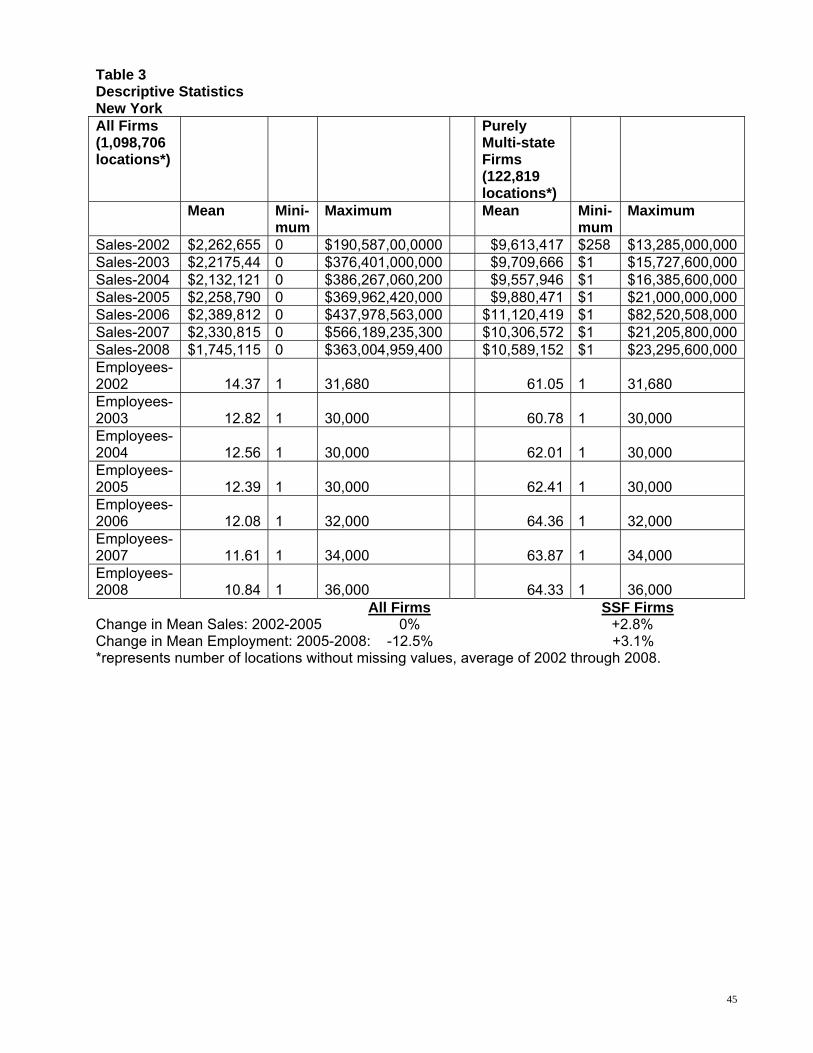
45

Table 3 Descriptive Statistics New York All Firms (1,098,706 locations*)


Mean Mini-mum


Maximum

Sales-2002 $2,262,655 0 $190,587,00,0000 $9,613,417 $258 $13,285,000,000Sales-2003 $2,2175,44 0 $376,401,000,000 $9,709,666 $1 $15,727,600,000Sales-2004 $2,132,121 0 $386,267,060,200 $9,557,946 $1 $16,385,600,000Sales-2005 $2,258,790 0 $369,962,420,000 $9,880,471 $1 $21,000,000,000Sales-2006 $2,389,812 0 $437,978,563,000 $11,120,419 $1 $82,520,508,000Sales-2007 $2,330,815 0 $566,189,235,300 $10,306,572 $1 $21,205,800,000Sales-2008 $1,745,115 0 $363,004,959,400 $10,589,152 $1 $23,295,600,000Employees-2002 14.37

1

31,680

61.05

1

31,680

Employees-2003 12.82

1

30,000

60.78

1

30,000


1

30,000

62.01

1

30,000


1

30,000

62.41

1

30,000


1

32,000

64.36

1

32,000


1

34,000

63.87

1

34,000


1

36,000

64.33

1

36,000

All Firms SSF Firms Change in Mean Sales: 2002-2005 0% +2.8% Change in Mean Employment: 2005-2008: -12.5% +3.1% *represents number of locations without missing values, average of 2002 through 2008.

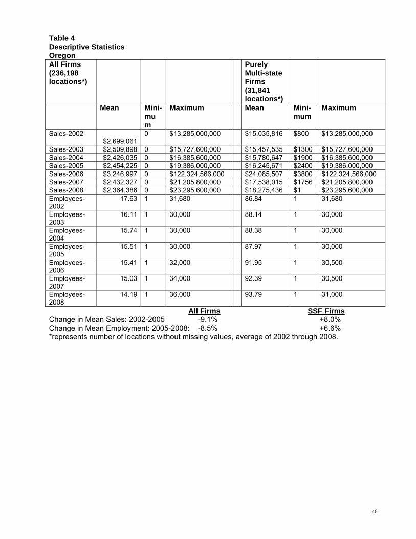
46

Table 4 Descriptive Statistics Oregon All Firms (236,198 locations*)


Mean Mini-mum


Maximum

Sales-2002 $2,699,061

0 $13,285,000,000 $15,035,816 $800 $13,285,000,000

Sales-2003 $2,509,898 0 $15,727,600,000 $15,457,535 $1300 $15,727,600,000 Sales-2004 $2,426,035 0 $16,385,600,000 $15,780,647 $1900 $16,385,600,000 Sales-2005 $2,454,225 0 $19,386,000,000 $16,245,671 $2400 $19,386,000,000 Sales-2006 $3,246,997 0 $122,324,566,000 $24,085,507 $3800 $122,324,566,000 Sales-2007 $2,432,327 0 $21,205,800,000 $17,538,015 $1756 $21,205,800,000 Sales-2008 $2,364,386 0 $23,295,600,000 $18,275,436 $1 $23,295,600,000 Employees- 2002

17.63 1 31,680 86.84 1 31,680

Employees- 2003

16.11 1 30,000 88.14 1 30,000

Employees- 2004

15.74 1 30,000 88.38 1 30,000

Employees- 2005

15.51 1 30,000 87.97 1 30,000

Employees- 2006

15.41 1 32,000 91.95 1 30,500

Employees- 2007

15.03 1 34,000 92.39 1 30,500

Employees- 2008

14.19 1 36,000 93.79 1 31,000

All Firms SSF Firms Change in Mean Sales: 2002-2005 -9.1% +8.0% Change in Mean Employment: 2005-2008: -8.5% +6.6% *represents number of locations without missing values, average of 2002 through 2008.

47

Table 5 Descriptive Statistics Wisconsin All Firms (298,675 locations*)


Mean Minimum Maximum Mean Minimum Maximum Sales-2002 $2,834,363 0 $13,285,000,000 $13,136,735 $200 $13,285,000,000 Sales-2003 $2,795,799 0 $15,727,600,000 $13,305,929 $400 $15,727,600,000 Sales-2004 $2,622,070 0 $16,385,600,000 $13,733,820 $400 $16,385,600,000 Sales-2005 $2,592,110 0 $19,386,000,000 $13,768,048 $500 $19,386,000,000 Sales-2006 $2,924,127 0 $122,324,566,000 $17,324,920 $500 $122,324,566,000Sales-2007 $2,505,768 0 $21,205,800,000 $14,586,134 $102 $21,205,800,000 Sales-2008 $2,381,445 0 $23,295,600,000 $15,036,254 $850 $23,295,600,000 Employees-2002

19.68 1 31,680 80.03 1 31,680

Employees-2003

18.96 1 30,000 79.25 1 30,000

Employees-2004

18.18 1 30,000 79.22 1 30,000

Employees-2005

17.69 1 30,000 79.63 1 30,000

Employees-2006

17.13 1 32,000 82.34 1 32,000

Employees-2007

16.67 1 34,000 82.61 1 34,000

Employees-2008

15.53 1 36,000 83.02 1 36,000

All Firms SSF Firms Change in Mean Sales: 2002-2005 -8.5% +4.8% Change in Mean Employment: 2005-2008: -12.2% +4.3% *represents number of locations without missing values, average of 2002 through 2008.

48

Table 6 Regression Results Georgia Parameter (expected sign)

Change in Sales (Model 1)


Sales (Model 3)

Change in Employ- ment (Model 1)

Change in Employ-ment (Model 2)

Employ-ment (Model 3)

Intercept .4222 (.0091)***

-.0184 (.0244)

3.459 (.0063)***

.0803 (.0009)***

.0097 (.0053)

.1247 (.0001)***

Locally-Based Multistate Firms (+)

6.372 (.0347)***

.4132 (.1413)***

2.691 (.0142)***

.2325 (.0032)***

.0414 (.01244)***

.1475 (.0018)***

Out of State Multistate Firms (+ or -)

-.5332 (.0307)***

-.1001 (.0385)***

-.8799 (.0165)***

-.0732 (.0060)***

-.0027 (.0080)

-.0193 (.0029)***

Industry Dummies Yes Yes Yes Yes Yes Yes Lagged Sales (+)

.5754 (.0007)***

Lagged Employment (+)

.8581 (.0009)***

Model F 11197.6*** 5.23*** 205600*** 1644.56*** 2.42** 1059676*** No. Observations 1,159,768 142,418 1,159,768† 1,159,768 142,418 1,159,768† Durbin-Watson D 1.264 1.715 ***significant at .001 or better **significant at .01 or better *significant at .05 or better † per year, 2002-2008 Sales and employment are in natural logs; standard errors (in parentheses) calculated using robust estimation methods

49

Table 7 Regression Results Louisiana Parameter (expected sign)



Sales (Model 3)




Intercept .3274 (.0123)***

-.0089 (.0138)

2.371 (.0086)***

.0722 (.0013)***

.0001 (.0069)

.0970 (.0007)***


6.5409 (.0513)***

.4642 (.1783)***

2.842 (.0188)***

.1767 (.0046)***

.1162 (.0397)***

.1218 (.0026)***


-.4780 (.0443)***

-.1487 (.0534)***

-.4566 (.0229)***

-.0857 (.0084)***

-.0144 (.0108)

-.0051 (.0042)

Industry Dummies Yes Yes Yes Yes Yes Yes Lagged Sales (+)

.6736 (.0001)***


.8687 (.0012)***

Model F 6111.39*** 5.54** 152834*** 509.29*** 2.91* 536801*** No. Observations 521,599 685,235. 521,599† 521,599 685,235 521,599† Durbin-Watson D 1.289 1.714 ***significant at .001 or better **significant at .01 or better *significant at .05 or better † per year, 2002-2008 Sales and employment are in natural logs; standard errors (in parentheses) calculated using robust estimation methods

50

Table 8 Regression Results New York Parameter (expected sign)



Sales (Model 3)




Intercept .1558 (.0059)***

.0737 (.0167)***

2.2810 (.0039)***

.0409 (.0006)***

.0085 (.0034)***

.0618 (.0003)***


6.654 (.0319)***

1.0568 (.1542)***

3.5104 (.0127)***

.1816 (.0030)***

.1361 (.0293)***

.1865 (.0017)***


-.3614 (.0270)***

-.2942 (.0324)***

-.4383 (.0141)***

-.0474 (.0052)***

-.0159 (.0065)**

.0152 (.0026)***

Industry Dummies Yes Yes Yes Yes Yes Yes Lagged Sales (+) .6382

(.0004)***


.8641 (.0006)***

Model F 5849.23*** 62.48*** 582431*** 1330.76*** 9.05*** 2467300*** No. Observations 2,395,613 230,036 2,395,613† 2,395,613 230,036 2,395,613† Durbin-Watson D 1.313 1.761 ***significant at .001 or better **significant at .01 or better *significant at .05 or better † per year, 2002-2008 Sales and employment are in natural logs; standard errors (in parentheses) calculated using robust estimation methods

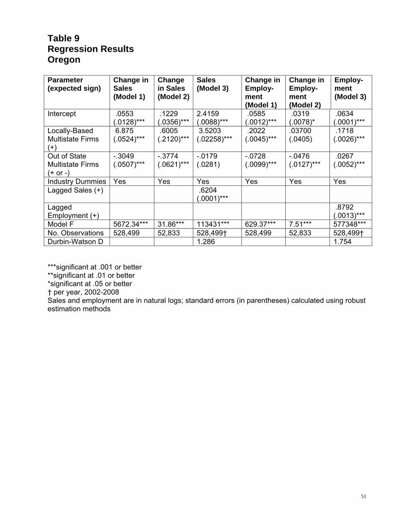
51

Table 9 Regression Results Oregon Parameter (expected sign)



Sales (Model 3)




Intercept .0553 (.0128)***

.1229 (.0356)***

2.4159 (.0088)***

.0585 (.0012)***

.0319 (.0078)*

.0634 (.0001)***


6.875 (.0524)***

.6005 (.2120)***

3.5203 (.02258)***

.2022 (.0045)***

.03700 (.0405)

.1718 (.0026)***


-.3049 (.0507)***

-.3774 (.0621)***

-.0179 (.0281)

-.0728 (.0099)***

-.0476 (.0127)***

.0267 (.0052)***


(.0001)***


.8792 (.0013)***

Model F 5672.34*** 31.86*** 113431*** 629.37*** 7.51*** 577348*** No. Observations 528,499 52,833 528,499† 528,499 52,833 528,499† Durbin-Watson D 1.286 1.754 ***significant at .001 or better **significant at .01 or better *significant at .05 or better † per year, 2002-2008 Sales and employment are in natural logs; standard errors (in parentheses) calculated using robust estimation methods

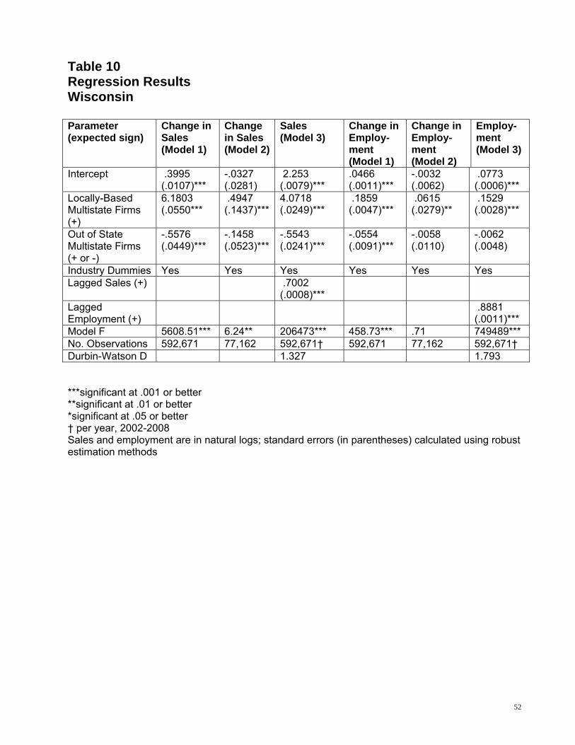
52

Table 10 Regression Results Wisconsin Parameter (expected sign)



Sales (Model 3)




Intercept .3995 (.0107)***

-.0327 (.0281)

2.253 (.0079)***

.0466 (.0011)***

-.0032 (.0062)

.0773 (.0006)***


6.1803 (.0550***

.4947 (.1437)***

4.0718 (.0249)***

.1859 (.0047)***

.0615 (.0279)**

.1529 (.0028)***


-.5576 (.0449)***

-.1458 (.0523)***

-.5543 (.0241)***

-.0554 (.0091)***

-.0058 (.0110)

-.0062 (.0048)


(.0008)***


.8881 (.0011)***

Model F 5608.51*** 6.24** 206473*** 458.73*** .71 749489*** No. Observations 592,671 77,162 592,671† 592,671 77,162 592,671† Durbin-Watson D 1.327 1.793 ***significant at .001 or better **significant at .01 or better *significant at .05 or better † per year, 2002-2008 Sales and employment are in natural logs; standard errors (in parentheses) calculated using robust estimation methods

53

Table 11 Regression Results All States Combined-Without State Tax Rates Parameter (expected sign)



Sales (Model 3)




Intercept .2641 (.0041)***

.0080 (.0124)

2.5921 (.0028)***

.0557 (.0004)***

-.0013 (.0025)

.0848 (.0002)***


6.1765 (.0214)***

1.0133 (.1325)***

3.2258 (.0085)***

.2093 (.0020)***

.1622 (.0255)***

.1677 (.0011)***


-.4393 (.0188)***

-.1932 (.0226)***

-.5536 (.0098)***

-.0603 (.0036)***

-.0040 (.0045)

.0116 (.0018)***

State has Throwback: Locally Based Firms (-)

-.2217 (.0582)***

-.4325 (.2241)*

-.8098 (.0246)***

-.0293 (.0050)***

-.0890 (.0446)*

-.0139 (.0030)***

State has Throwback: Out of State Based Firms (-)

-.0191 (.0483)

-.0098 (.0491)

.1781 (.2066)

-.0079 (.0097)

-.0077 (.0099)

.0164 (.0501)

State is Unitary: Locally Based Firms (+)

.3648 (.0745)***

.7184 (.3081)*

.7068 (.0319)***

.0289 (.0064)***

.0700 (.0776)

.0011 (.0060)*

State is Unitary: Out of State Based Firms (+)

-.0827 (.0684)

-.0884 (.0694)

.-0768 (.0374)***

-.0069 (.0314)

-.0885 (.0136)

.0053 (.0070)


(.0003)***


.8553 (.0004)***

Model F 13238.3*** 26.41*** 490762*** 1650.41*** 5.47*** 1975041*** No. Observations 5,080,596 504,192 5,080,596† 5,080,596 504,192 5,080,596† Durbin-Watson D 1.319 1.720 ***significant at .001 or better **significant at .01 or better *significant at .05 or better † per year, 2002-2008 Sales and employment are in natural logs; standard errors (in parentheses) calculated using robust estimation methods

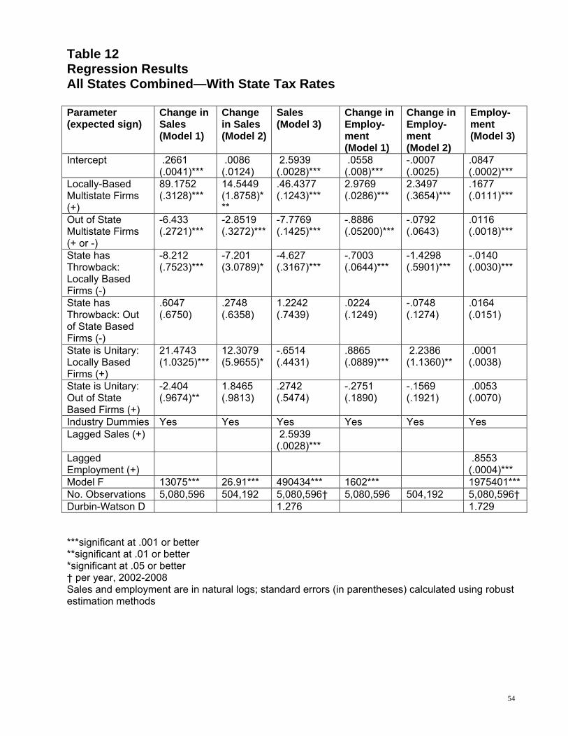
54

Table 12 Regression Results All States Combined—With State Tax Rates Parameter (expected sign)



Sales (Model 3)




Intercept .2661 (.0041)***

.0086 (.0124)

2.5939 (.0028)***

.0558 (.008)***

-.0007 (.0025)

.0847 (.0002)***


89.1752 (.3128)***

14.5449 (1.8758)***

.46.4377 (.1243)***

2.9769 (.0286)***

2.3497 (.3654)***

.1677 (.0111)***


-6.433 (.2721)***

-2.8519 (.3272)***

-7.7769 (.1425)***

-.8886 (.05200)***

-.0792 (.0643)

.0116 (.0018)***

State has Throwback: Locally Based Firms (-)

-8.212 (.7523)***

-7.201 (3.0789)*

-4.627 (.3167)***

-.7003 (.0644)***

-1.4298 (.5901)***

-.0140 (.0030)***

State has Throwback: Out of State Based Firms (-)

.6047 (.6750)

.2748 (.6358)

1.2242 (.7439)

.0224 (.1249)

-.0748 (.1274)

.0164 (.0151)

State is Unitary: Locally Based Firms (+)

21.4743 (1.0325)***

12.3079 (5.9655)*

-.6514 (.4431)

.8865 (.0889)***

2.2386 (1.1360)**

.0001 (.0038)

State is Unitary: Out of State Based Firms (+)

-2.404 (.9674)**

1.8465 (.9813)

.2742 (.5474)

-.2751 (.1890)

-.1569 (.1921)

.0053 (.0070)

Industry Dummies Yes Yes Yes Yes Yes Yes Lagged Sales (+) 2.5939

(.0028)***


.8553 (.0004)***

Model F 13075*** 26.91*** 490434*** 1602*** 1975401*** No. Observations 5,080,596 504,192 5,080,596† 5,080,596 504,192 5,080,596† Durbin-Watson D 1.276 1.729 ***significant at .001 or better **significant at .01 or better *significant at .05 or better † per year, 2002-2008 Sales and employment are in natural logs; standard errors (in parentheses) calculated using robust estimation methods

55

Figure 1

Income Effect of Single Sales Versus Double-Weighted Sales: Locally-Based Firm

Double-

Weighted Single

Sales Payroll 80% 80% Property 80 80 Sales 20 20 Apportionment ratio 50% 20% X Total U.S. profits (millions) $10.0 $10.0 = State taxable profits (millions) 5.0 2.0 State Tax Payment at 8 Percent $400,000 $160,000

Figure 2

Income Effect of Single Sales Versus Double-Weighted Sales: Out-of-State Firm

Double-

Weighted Single

Sales Payroll 4% 4% Property 4 4 Sales 14 14 Apportionment ratio 9% 14% x Total U.S. profits (millions) $10.0 $10.0 = State taxable profits (millions) 0.9 1.4 State Tax Payment at 8 Percent $72,000 $112,000

56

Figure 3

Inter-State Production Model

State 1 Operations

λQ1 Labor L1 Intermediate Output Capital K1

Finished Output Q1

Sold to State 1 & 3 Consumers

State 2 Operations λQ2

Intermediate Output Finished Output Q2 Sold to State 2 & 4 Consumers Labor L2 Capital K2

Parent Company

Subsidiary S1

Subsidiary S2

on the effectiveness of single sales … on the effectiveness of single sales factors for state...

Documents