HAL Id: hal-00003478https://hal.archives-ouvertes.fr/hal-00003478

Preprint submitted on 7 Dec 2004

HAL is a multi-disciplinary open accessarchive for the deposit and dissemination of sci-entific research documents, whether they are pub-lished or not. The documents may come fromteaching and research institutions in France orabroad, or from public or private research centers.

L’archive ouverte pluridisciplinaire HAL, estdestinée au dépôt et à la diffusion de documentsscientifiques de niveau recherche, publiés ou non,émanant des établissements d’enseignement et derecherche français ou étrangers, des laboratoirespublics ou privés.

On the diffraction pattern of C60 peapodsJulien Cambedouzou, Vincent Pichot, Stéphane Rols, Pascale Launois, Pierre

Petit, Robert Klement, Hiromichi Kataura, Robert Almairac

To cite this version:Julien Cambedouzou, Vincent Pichot, Stéphane Rols, Pascale Launois, Pierre Petit, et al.. On thediffraction pattern of C60 peapods. 2004. �hal-00003478�

ccsd

-000

0347

8, v

ersi

on 1

- 7

Dec

200

4

On the diffraction pattern of C60 peapods.

J. Cambedouzou1, V. Pichot2, S. Rols1, P. Launois2, P.

Petit3, R. Klement3,4, H. Kataura5 and R. Almairac1

1Groupe de Dynamique des Phases Condensees (UMR CNRS 5581),

Universite Montpellier II, 34095 Montpellier Cedex 5, France

2Laboratoire de Physique des Solides (UMR CNRS 8502),

Universite Paris Sud, 91405 Orsay

3Institut Charles Sadron, 67000 Strasbourg, France

4Department of Physical Chemistry,

Faculty of Chemical and Food Technology,

Slovak Technical University, Radlinskeho 9,

812 32 Bratislava, Slovak Republic and

5Nanotechnology Research Institute,

National Institute of Advanced Industrial Science and Technology (AIST) Central 4,

Higashi 1-1-1, Tsukuba, Ibaraki 305-8562, Japan

(Dated: December 7, 2004)

Abstract

We present detailed calculations of the diffraction pattern of a powder of bundles of C60 peapods.

The influence of all pertinent structural parameters of the bundles on the diffraction diagram is

discussed, which should lead to a better interpretation of X-ray and neutron diffraction diagrams.

We illustrate our formalism for X-ray scattering experiments performed on peapod samples syn-

thesized from 2 different technics, which present different structural parameters. We propose and

test different criteria to solve the difficult problem of the filling rate determination.

PACS numbers: 61.46.+w,61.10.Dp,61.10.Nz

1

I. INTRODUCTION

Since their discovery in 1991 [1], carbon nanotubes have been the purpose of a large

number of studies, dealing both with their mechanical and electronic properties. In

particular, it has been shown that the intercalation of electron donors or acceptors [2, 3, 4]

into single wall carbon nanotubes (SWNT) bundles could dramatically modify the electronic

properties of these objects. Rather large molecules are expected to be inserted into the

hollow core of a nanotube that has been shown to present very stable adsorption sites

[5]. C60 is one of the molecules that have successfully been inserted into SWNT, and a

lot of studies have recently been achieved on the so-called ”peapods”. Those systems

consist of SWNT in which C60 fullerene molecules are inserted [6]. Their study stands

within the fascinating field of systems in a confined geometry [7, 8, 9, 10]. Peapods

structural analysis can be performed on a small number of tubes (and even on a single

tube), using transmission electron microscopy (TEM) [6, 11] or electron diffraction [12, 13],

or on macroscopic assemblies, using Raman spectroscopy [11, 14, 15] or X-ray scattering

[15, 16, 17].

Theoretical and experimental studies have already been published on the diffraction dia-

gram of powder of SWNT bundles [18, 19]. In particular, the importance of the distribution

of tube diameter on the position of the (10) Bragg peak in the X-ray and neutron diffrac-

tion patterns was pointed out in ref. [19, 20]. The complete study of the influence of all

structural parameters of the bundles was performed using a simple numerical model. It was

shown that modeling is essential for a correct determination of the structural parameters for

such inhomogeneous samples of fairly crystallized nano-objects. Intercalated SWNT bundles

form even more complex nano-crystalline systems. The adsorption sites can be separated

into 3 main locations: inside the tubes, on the outer surface of the bundles (including the

so-called ”grooves”[5]) and into the interstitial channels of the 2D triangular lattice. Ad-

sorption of a molecule into a SWNT bundle can involve modifications of the 2D triangular

lattice (symmetry and/or lattice parameter expansion). These modifications lead to site-

dependent diffraction diagram governed by the structure of the host (the nanotube bundle),

the structure of the adsorbed species inside the bundles and by crossed interferences between

the host and the molecules adsorbed. The modifications of the diagrams are also found to be

2

radiation dependent [21]. Therefore, an efficient and correct interpretation of the diffraction

diagram from such complex systems requires the use of simulation.

The study of the structure of C60 (and C70) peapods by X-ray diffraction has recently been

achieved by Kataura, Maniwa and co-workers [15, 16]. The authors could estimate the C60

(and C70) filling rates from the analysis of their measurements. Also, the 1D lattice con-

stant of the C60 chains inside the tubes was found to be smaller than those for 3D crystals

of C60. More strikingly, the temperature dependence of the corresponding feature in the

diffraction diagram shows no dependence, indicating a nearly zero thermal expansion of the

C60 chain inside the tubes, raising questions about possible polymerization of the C60 chains.

X-ray diffraction is found to be a very powerful tool to probe the structure of C60 inside

the tubes. However, further experimental work is needed to understand the properties of

C60 peapods. Such experimental work should include diffraction investigations on samples

showing peapods having various structural characteristics:

1. different tube diameters

2. different filling rates

3. bundles with various sizes e.g. various numbers of tubes

and particularly, to allow variable degrees of freedom for the fullerene molecules. Therefore,

in this paper, we propose to give a detailed ”step by step” and complete study of the diffrac-

tion patterns of peapods and we discuss the characteristic signatures linked to the insertion

of C60 inside the SWNTs. We also show how the variation of different structural parameters,

such as tube diameter, filling rate of SWNTs by C60, and C60 adsorption in the outer groove

sites at the surface of the bundles can change the shape of the diffraction pattern. The

reader has to keep in mind that this report is an attempt to give experimentalists the nec-

essary tools to characterize their samples by X-ray and/or neutron diffraction. Very often

it appears that unexpected impurity phases are present in SWNT samples, as revealed by a

comparison between X-ray and neutron diffraction patterns measured on the same powder.

Therefore both techniques are complementary. In the first part of this paper, we present the

theoretical model used to achieve the simulations. We consider a powder of uncorrelated

tubes filled with C60 in the second part, and the third part deals with powder of bundles of

peapods. Polymerization of the C60 chains is also considered. We finally compare the results

3

of our calculations with experimental diffraction patterns. A large part of the discussion is

concerned with the determination of the filling rate in the investigated samples.

II. PRINCIPLE OF THE CALCULATIONS

In our attempt to reproduce the diffraction pattern of peapods, we developed a model

based on the general equations for x-ray and neutron diffraction in the kinematical approx-

imation [22, 23] for which the diffracted intensity is proportional to the squared modulus of

the scattering amplitude. The latter is defined as the Fourier transform of a configuration

of atoms in the scattering volume. The diffracted intensity thus writes as follows:

I( ~Q) ∝

∣

∣

∣

∣

∫

volume

fsρ(~r)ei ~Q·~rd3~r

∣

∣

∣

∣

2

(1)

where ~Q is the scattering vector, ρ(~r) is the density of scatterer at position ~r in the

sample, and fs depends both on the scattering element (e.g the atomic species) and on the

nature of the incident radiation (fs is a function of the wave-vector modulus Q for X-rays

while it is constant for neutrons). Since we consider the case of a powder experiment, the

diffraction is to be averaged over all the directions of space or, equivalently, over all the

orientations of the scattering vector in the reciprocal space. The mean diffracted intensity

is thus given by:

I(Q) =

∫ ∫

I( ~Q)d2S( ~Q)

4πQ2(2)

where the integration is performed over the sphere of radius Q and d2S( ~Q) is a surface

element of this sphere. Therefore, the model consists in choosing a convenient -and physically

correct- mathematical form of the density of scatterer ρ(~r). A powerful approach consists

in replacing the discrete carbon atoms by uniformly charged surfaces for both nanotubes

and C60 molecules, with a surface atomic density σc ∼ 0.37 atom/A2. This value is a little

underestimated for C60 molecules (∼ 0.39 atom/A2) but we take it as equal for the simplicity.

This assumption results in a loss of information concerning the atomic arrangement at the

surface of the objects forming the sample. It limits the reliability of our results to Q-values

lower than 2 A−1. Below this value, the diffraction pattern is indeed insensitive to the

detailed atomic order. It is however very much affected in this Q range by the medium

range organization e.g. the 2D hexagonal nanotubes bundles and the 1D C60 packing. In

the following, we will therefore be concerned with the two latter levels of organization in the

4

framework of the homogenous approximation.

The detailed parameters of the model and the definition of the different variables used

thorough this work are presented in Figure 1:

• The upper part represents a single tube filled with a linear chain of C60s. Each C60-

filled nanotube will be considered as a linear superposition of 1D unit cell, each cell

consisting of a cylinder of length L and of a single C60 molecule located at its center.

• The lower part represents the peapods organized into bundles e.g. on a 2D hexagonal

lattice, the parameter of which is a function of the tubes diameter forming it. We

introduced a random shift Tz between the position of the C60 molecules on one tube

with respect to the corresponding position on the central tube to avoid unrealistic

correlations between the positions of the C60s inside the different nanotubes of the

same bundle.

III. ISOLATED TUBES FILLED WITH A CHAIN OF C60 MOLECULES: ISO-

LATED PEAPODS.

A. Complete filling of the nanotubes

In this part, we discuss the main features of the diffraction pattern calculated for a powder

of 380 A long and 13.6 A large peapods that is obtained by stacking 40 cylinders of length

9.5 A, each cylinder containing a 3.5 A radius sphere at its center (see Figure 1). This value

of 9.5 A is not deduced from measurements. It must be considered as a parameter of the

model. We present in figure 2 the calculated intensity for this object (bottom), for the tube

alone (top) and for a C60 chain alone (middle).

Let It be the intensity diffracted by a powder of empty nanotubes. It is a pseudo-periodic

oscillating function which is proportional to the squared modulus of the zero order cylindrical

Bessel function J0 , as it appears in the following expression of It:

It(Q) ∝

∫ π

u=0

∣

∣

∣At( ~Q)

∣

∣

∣

2

sin(u)du (3)

with At the amplitude scattered by the empty nanotube:

At( ~Q) = 2πLrhfsσcJ0(Qrhsin(u))sin(QL

2cos(u))

QL2cos(u)

40∑

n=0

eiQnLcos(u) (4)

5

and where u, L and rh are defined in figure 1 and where n labels the 1D unit cells (cylinders

of length L).

Let Ic be the intensity diffracted by a powder of linear chains of C60 molecules:

Ic(Q) ∝

∫ π

u=0

∣

∣

∣Ac( ~Q)

∣

∣

∣

2

sin(u)du (5)

where Ac is the amplitude scattered by the linear chain of C60 molecules:

Ac( ~Q) = 4πr2C60

fsσcsin(QrC60)

QrC60

40∑

n=0

eiQnLcos(u) (6)

and where rC60 is the radius of a C60 molecule (3.5 A). This intensity is also a pseudo-periodic

oscillating function, but with a pseudo-period that is nearly twice as long as the one of the

nanotubes. Indeed, the radius of a C60 is nearly half the radial dimension of the tube.

Another interesting feature of the latter curve is the asymmetric peak at 0.68 A−1 , which

results from the periodic positions of C60s along the linear chain [24].

The first minimum of the intensity diffracted by the whole peapod (pointed by an arrow in

fig.2) is located at Q=0.44 A−1 , whereas it was located at 0.38 A−1 in the empty SWNT

diffraction pattern. Following the work on gas adsorption inside SWNT by Maniwa et al.

[25], H. Kataura et al. gave a simple explanation for this feature [15]: the reason for the

presence of this minimum at this precise value of Q is due to the sum of the structure factors

of the tube and of the C60 which equals zero for Q=0.44 A−1. We will discuss this effect in

slightly different term. Let us write the intensity Ip(Q) diffracted by a peapod as follows:

Ip(Q) ∝

∫ ∫

∣

∣

∣At( ~Q) + Ac( ~Q)

∣

∣

∣

2

d2 ~Q (7)

According to the fact that At and Ac may be complex, relation ( 7) can be developed as:

Ip(Q) ∝ It(Q) + Ic(Q) + 2

∫ ∫

[

Re(At( ~Q))Re(Ac( ~Q)) + Im(At( ~Q))Im(Ac( ~Q))]

d2 ~Q (8)

where Re(At) and Im(At) stand for the real and imaginary parts of At, respectively.

Relation (8) can be rewritten as:

Ip ∝ It + Ic + ICI (9)

If attention is given to figure 2c, it is clear that the profile of Ip is quite different from (It+Ic).

This latter quantity is indeed the signature of a sample containing a tube decorrelated from

6

a linear chain of C60. In a peapod sample, there is a strong correlation in the relative

positions of the tube and the chain of C60, since the C60s are located inside the tube.

This correlation is revealed by the presence of the crossed interference term ICI which can

be positive or negative. At Q=0.44 A−1, the crossed term compensates the (It+Ic) term,

lowering Ip to zero or nearly zero [26]. This value for Q is accidently the same as that of the

(10) peak position for a bundle made of empty SWNTs stacked into a 2D hexagonal lattice.

This coincidence will cause dramatic changes in the diffraction pattern relative to peapods

bundles (see part IV).

The increase of the tube diameter induces a decrease of the oscillation period as it is expected

when considering larger diffracting object (see figure 3). The C60 periodicity characteristic

peak at 0.68 A−1, as well as its first harmonic at 1.36 A−1, are observable in all the calculated

diffraction profiles. For peapods of radius r=5.42 A (for example C60@(8,8) peapods) the first

peak is not separated from the first oscillation, but is clearly visible. The same behavior is

observed for r=8.1 A peapods (for example C60@(12,12) peapods) on the second oscillation,

but the peak amplitude is weaker. In fact, the larger the tube diameter and the weaker this

peak. The latter effect can be easily understood: an increase of the tube diameter implies

an increase of the tube surface which leads to a preponderance of the response of the tubes

over the response of the C60 chains, in which the number of scatterers remains unchanged.

The cases of C60@(8,8) and C60@(12,12) peapods are discussed here as extreme cases for the

influence of the tube diameter. However, it must be pointed out that the insertion of C60

in a (8,8) peapod is unlikely due to the too small diameter of the tube, and C60s inside a

(12,12) peapod would possibly lead to zigzag or helical chains in place of linear chains, since

the center of the tube is no longer the most favorable location for C60 regarding to van der

Waals interactions.

The bottom part in figure 3 reveals the consequences of a change in the inter-C60 length L

inside the linear chain. A downshift of the characteristic peak of C60s periodicity is evidently

observed when L increases, but we also note a reinforcement of its intensity. One remarks a

striking effect: although the relative density of C60 increases, the characteristic peak relative

to the C60 periodicity strongly decreases. This is due to the multiplication factor arising

from the intensity diffracted by a C60 molecule, which reaches its first zero at 0.9 A−1, as

shown in figure 2. The closer the peak position to this value, the weaker the peak. One

must be careful with the fact that the respective proportion between tube and C60s is no

7

longer the pertinent parameter to account for the explanation of the changes in the peak

intensities. Thus, it may prove dangerous to focus only on the relative intensity of this peak,

and it seems necessary to consider the whole diffraction pattern to derive reliable structural

information.

In several cases, the use of an analytical formula can prove more comfortable than the method

presented above. For infinite tubes, numerical calculations are performed after the limit of

infinite tube length was taken in the above equations, leading to the following equation

(demonstrated in appendix 1 eq. 16), where the first term comes from the Fourier transform

of the structure projected in a plane perpendicular to the tube axis, while the second one

comes from the periodicity of the C60 chains:

Ip(Q) ∝f 2

s

Q

(

(2πLrhσcJ0(Qrh) + 4πr2C60

σcsin(QrC60)

QrC60

)2 + 2Int(QL

2π)(4πr2

C60σc

sin(QrC60)

QrC60

)2

)

(10)

In this expression Int(QL2π

) is the integer part of (QL2π

).

B. Partial filling of the nanotubes

In the case of a real sample, it seems reasonable to consider that all tubes may not be

fully filled with C60s, despite efforts made to obtain filling rates as high as possible [11].

Two different hypotheses are discussed here.

The first hypothesis is to consider a random filling of the tubes without assuming clustering

effects inside the tubes : the molecules are randomly positioned within a tube, the only

constraint being a minimum distance of L between them (one may note that it implies

that in the limiting case of 100% filling, the molecules necessarily form ordered chains).

Calculations are performed within the finite tube length model, for a given filling ratio of

the nanotubes. The effects of a random incomplete filling of the nanotubes are presented in

the upper part of figure 4. One observes the vanishing of the C60-C60 characteristic peak with

decreasing filling rates; it completely disappears for filling rates below 85%. If we compare

the shapes of the 85% and the 100% diffraction profiles, one finds that the minimum at

0.44 A−1 for the 85% filled sample no longer lowers to zero. The additional intensity can

be attributed to the effect of the disorder induced by the random filling of the nanotubes

by the C60 molecules. Moreover, the first minimum in intensity shifts to lower Q values for

8

decreasing rate of fullerenes, which can be explained as in figure 2 by compensation effects

between tube, fullerene and interference terms.

As a second hypothesis, one can consider the partial filling of the tubes with long (’quasi-

infinite’) chains of C60. We assume here that the molecules tend to cluster within nanotubes.

Indeed, this should correspond to a low energy configuration of the system, the energy being

lowered by the attractive C60-C60 interactions. This hypothesis is supported by observations

reported in ref. [13]. Calculated diffraction patterns for different filling rates (50%, 75% and

100%) are presented in the lower part of figure 4. Here we use the infinite tube length model

(detailed calculations are given in appendix 2). As it was already mentioned in the first

hypothesis, we observe the vanishing of the C60-C60 characteristic peak at low filling rates,

but it interestingly disappears here for a filling rate of 50% which is much lower than the 85%

observed in the first part. This is due to the long chains assumption : the C60-C60 distance

is preserved for the different filling rates. Another feature of these diffraction patterns is

that the first minimum goes to zero for all filling rates, contrarily to what was found within

the first hypothesis, which is due to lower disorder.

If one takes into account the differences pointed out between the 2 hypothesis discussed

here, one should in principle be able to determine the way a sample of isolated peapods is

filled. Unfortunately, the Q range around 0.44 A−1 is usually perturbed by parasitic signals

(intense scattering at small wave-vectors ), so it is very difficult to use the value of the

first minimum of intensity as a clue to determine the filling mode. As a result, the C60-C60

characteristic peaks remain the only observable features for the estimation of the filling rate

and of the filling mode. An important result from our calculations is that C60 molecules in

isolated peapods with a random filling rate below 85% and peapods with a long chain filling

rate under 50% are undetectable by diffraction.

C. Polymerized C60 molecules inside nanotubes

One of the remarkable properties of the C60 molecule is its ability to form covalent

bonds through quite different routes. In crystalline C60, polymers can be obtained (i) by

photopolymerization, (ii) under pressure and at high temperature , (iii) in doped samples

[27, 28]. Photo-induced [11, 15] and charge transfert induced [29] polymerization have also

been demonstrated in C60 peapods, using Raman spectroscopy. It is interesting to consider

9

the effect of polymerization on diffraction patterns. Let us consider peapods where the chains

can be formed of n-polymers (n=1: monomers, n=2: dimers, n=3: trimers...). For the sake

of simplicity, we deal with the case of completely filled nanotubes. The distance Lb between

bonded C60 molecules is taken to be 9.2A as in crystalline polymerized samples, and the

distance L between unbonded molecules is fixed at 9.5A as above. The distance between

monomers is smaller in peapods than in crystalline C60, where it is equal to about 10A,

possibly because of interactions with the nanotubes. However, there is no reason to take a

smaller value for the distance between bonded molecules because it is mainly determined by

the covalent bonding between them. It is shown in appendix 3 that the scattered intensity

of a powder of peapods filled with chains of n-polymers writes:

Ip(Q) ∝f 2

s

Q((2πrh(L + (n − 1)Lb)σcJ0(Qrh) + 4πr2

C60σcn

sin(QrC60)

QrC60

)2

+2(1 − δM,0)M∑

k=1

(4πr2C60

σcsin(QrC60)

QrC60

sin(kπnLb/(L + (n − 1)Lb))

sin(kπLb/(L + (n − 1)Lb)))2) (11)

where the second term appears only for Q values such that M -the integer part of

(Q(L+(n−1)Lb)2π

) - is not zero. Calculated patterns for n=1, 2 and 3 are drawn in fig.5. At

each Q = k2π/(L+(n−1)Lb) value (with k integer), asymmetric peaks characteristic of the

chain periodicity can be observed. Despite the change of the period -equal to (L+(n-1)Lb)

- with n, the spectra look quite similar. It can easily be explained from eq. 11 : the asym-

metric peak intensity is multiplied by[

sin(kπnLb/(L+(n−1)Lb))sin(kπLb/(L+(n−1)Lb))

]2

, which is close to zero except

for k=n, 2n,... The first intense peak of the n-polymer diffraction pattern is thus located

at Q=n2π/(L + (n − 1)Lb) : Q=0.672A−1 for dimers, 0.676 A−1 for trimers, to be com-

pared with 0.661A−1 for monomers. The upper value, corresponding to infinite polymers, is

Q=2π/9.2 =0.683A−1.

In summary, scattering analysis of polymerization of C60 molecules in peapods samples

should be based on a careful study of the position Q0 of the first intense asymmetric peak,

and on the search for lower intensity peaks at kQ0/n (n=2,3...; k=1 to (n-1)) to identify

n-polymers.

10

IV. BUNDLES OF PEAPODS.

A. Complete filling

Peapods are packed into bundles where they are maintained together by van der Waals

inter-tubes interactions. This organization is clearly visible on TEM pictures [11, 15, 16]. In

this part, we calculate and discuss the diffraction pattern for such objects. Calculations are

performed both for peapods of finite length and for peapods of infinite length (as detailed

in appendices 1 and 2). The relative positions of the C60 chains along the tube axes (Tz in

fig.1) are assumed to present no correlation from one tube to another. Indeed, a C60 chain

interacts the most with the nanotube in which it is located, and nanotubes within a bundle

present different helicities [30].

Figure 6 shows the comparison between the diffraction profiles calculated for a powder of

bundles of 12 empty nanotubes and that of bundles of 12 peapods, with different tube radii.

In all cases, we consider 380 A long nanotubes organized on a 2D hexagonal lattice with a 3.2

A van der Waals length between 2 adjacent nanotubes. Let us first consider the upper part

of figure 6, which deals with (10,10) tubes and peapods, of radius r=6.8 A. For peapods,

the additional peaks characteristic of the 1D periodicity of the C60 chains are indicated

by an arrow. We remark that most of the characteristic peaks observed in the diffraction

pattern of the empty SWNT bundles show up in the diffraction pattern of the peapod

bundles, except those located in the low Q range where a lack of intensity is obtained for the

peapods. An important difference between the pattern of the peapod bundles and the empty

nanotube bundles is thus the disappearance of the (10) Bragg peak at 0.44 A−1. This peak

(of finite width because of the small bundle size) is replaced by a minimum delimited by two

smaller peaks. This can be explained on the basis of part III results, since we observed that

the intensity diffracted by a single peapod lowers to zero at 0.44 A−1, which is around the

position of the (10) lattice peak of the bundles. This important extinction process in the case

of SWNT bundles has already been found and discussed for different kinds of intercalated

molecules like gas molecules [15, 31] or in iodine doped nanotubes samples [21]. Middle

and lower parts of figure 6 show that the extinction phenomenon is modified when the tube

diameter is changed. For example, we consider the case of bundles of 12 empty nanotubes

and 12 peapods of radius r=5.42 A ((8,8) tubes, middle part of figure 6) and r=8.1 A ((12,12)

11

tubes, lower part of figure 6). One can see that the (10) peak is not split into two parts for

the bundle of (8,8) peapods, but appears shifted to lower Q values. By contrast, this peak

completely disappears in the case of the bundle of (12,12) peapods. When tube is thinner

or larger in diameter, the progressive loss of the accidental adequate conditions implies the

extinction phenomenon to be lost.

It is important to be aware that the extinction can occur for values of Q that are slightly

different from the (10) peak position. In that case the (10) peak does not appear split, but

seems shifted because only one side of the peak is lowered. Therefore, a direct interpretation

of such apparent shift in terms of a change of the lattice parameter is inappropriate, and

direct conclusions about structural changes based on the observation of the (10) peak alone,

prove very hazardous. The analysis of peapods diffraction patterns is consequently not

straightforward and should be based on comparison between measurements and calculations.

B. Partial filling

As for isolated tubes, all tubes may not be fully filled with C60s. In this part, 4 different

filling modes are discussed.

The first case (case a) consists in a random filling, where each tube of the bundle is filled as

described in part III.B. Calculations are performed within the finite tube length model. In

the 3 other cases, which are treated within the infinite tube assumption (detailed calculations

are given in appendix 2), the C60s are all stacked into long chains, but the way these

chains are distributed into the bundles changes with the case. One can indeed consider an

homogeneous filling (case b), where the tubes are all filled with the same number of C60

molecules, or an inhomogeneous filling (case c), where the filling rate of each tube of the

bundle is slightly different. The last case to be discussed (case d) consists in a mix of fully

filled bundles and empty bundles (see the right part of figure 7).

We present the results for filling rates of 85% and 50% for bundles of 12 nanotubes of radius

r=6.8A in the left part of figure 7. The main difference between all diffraction patterns

calculated for a 85% filling rate and all those calculated for a 50% filling rate is visible in

the low Q range. The (10) Bragg peak is indeed still splitted and almost invisible at the

85% filling rate, while it clearly reappears at the 50% filling rate. This observation can be

explained by the fact that the accidental conditions allowing the extinction of the (10) Bragg

12

peak are progressively lost when the proportion of C60 decreases in the sample.

If more attention is given to the a), b), c) and d) diffraction profiles for a given filling rate,

other features linked to the different filling modes can be extracted from the figure. One

can first consider the Q range below 0.6 A−1. The intensity in this region is the least for

the b) configuration, which is the least disordered configuration. If we compare with the

inhomogeneous filling (mode c), and then with the random filling (mode a), we observe a

progressive increase of the intensity in the low Q range, corresponding to the progressive

increase of the disorder in the system, as already mentionned in part III.B. The d) case must

be considered separately from the other cases because the intensity in the low Q range is here

the sum of the intensities of 2 decorrelated systems ( full peapods and empty nanotubes).

One can also focus on the C60-C60 characteristic peak. This asymmetric peak is clearly visible

on the diffraction profiles of the b), c) and d) filling modes, even for the 50% filling rate,

whereas it never appears at this rate for isolated peapods. In addition, this peak is invisible

at both filling rates in the a) filling mode. Thus, the observation of such a feature in an

experimental diffraction pattern should stand as the signature of a long chain organization

of the C60 molecules inside the tubes.

C. Chains of C60 molecules in the outer groove sites of the bundles

We finally discuss the effects induced by the filling of the channels located at the bundle

surface with linear chains of C60s , for bundles of various size (figure 8). All tubes have

a radius of 6.8 A. When we consider the diffraction pattern of a 6 peapods bundle where

the external channels have been completely filled, we note 2 main differences with regards

to a naked peapod bundle. First, the peak at 0.68 A−1 is significantly reinforced due to

the additional C60 molecules in the external channels. Secondly, the intensity in the low

Q range as well as between 1 and 1.5 A−1 appears strengthened. As it is shown in figure

2, the C60 response is high in these Q ranges, so this effect is just due to the increase of

the C60 proportion in the sample. It is evidently clear that the higher the number of tubes

in the bundle, the weaker the effect described just above. The reason for that lies in the

simple fact that volume grows faster than surface when the size of the bundle increases.

According to these results, we are able to conclude that an experimental diffraction pattern

with a high intensity in the 1 to 1.5 A−1 Q range may be relative to a sample made of small

13

sized bundles, saturated with C60s in both the inner space of the tubes and in the external

channels.

D. Determination of the filling rate

In this section we try to define a method to determine the filling rate from experimental

data. Two criteria are proposed which are based on the analysis of the results obtained

from the model. As it was explained previously, the (10) Q range is strongly perturbed, so

this Q range is disregarded. The first criterion consists to remark that the peak centered

around 0.7 A−1 contains two contributions (fig. 7): i) the response of the C60 lattice at

0.663 A−1 and ii) the (20) reflection of the bundle lattice centered at 0.706 A−1 . The

ratio of the two respective amplitudes is expected to vary as a function of the filling rate.

However two problems arise. The first one concerns the type of filling which is unknown.

The second concerns the background determination. We assume that the background can

be represented by a straight line between 0.6 A−1 and 0.8 A−1 as is shown in the inset of

fig. 9a. In fig. 9a the amplitude ratio is drawn as a function of the filling rate and for the

two extrem types of filling, i.e. random and homogeneous (a) and b) cases, respectively).

Cases c) and d) have intermediate behaviors, so they are not presented in this figure. Thus

for a given experimental amplitude ratio (on vertical axis) one gets a range for the filling

rate.

The second criterion consists to use: i) the amplitude of the C60 1-D lattice peak around

1.3 A−1 as this peak arises in a Q range where the C60 contribution is strong, and ii) the

amplitude of the (21) reflection of the bundles around 1.1 A−1 as the C60 contribution is

small in this Q range. The calculated diagrams of fig. 7 were analyzed with a 3 peaks model

from which we extracted the two amplitudes (fig. 9b). Again the background estimation

has a large incidence on the results.

The second criterion seems to be more reliable as it presents a smaller dependence on the

type of filling. It is of easier use. However it has been established for SWNT bundles

corresponding to diameters occuring in the case of electric arc or laser synthesis, i.e.

centered around 1.4 nm and with a small dispersion in diameter distribution (FWHM ≤ 2

A ). In the next section these criteria are applied to the estimation of the filling rate in two

14

different samples.

V. COMPARISON BETWEEN CALCULATED AND EXPERIMENTAL

DIFFRACTION PATTERNS

Diffraction patterns were performed using a powder diffractometer equiped with a curved

position sensitive detector INEL CPS120 allowing one to measure simultaneously a range

of 2θ angles from 2 to 120◦. A wavelength of 1.542 A was used. We measured the diffrac-

tion pattern of two different peapod samples (powder sample or numerous small pieces of

bucky paper in glass capillaries). Sample A (figure 10a) was synthesized as follows : the

SWNT material was first soaked in concentrated nitric acid (HNO3 65%) and sonicated for

approximatively 30 min, then treated in boiling HNO3 at 140-150 ◦C for 4 hours. After

sedimentation of the acid treated SWNT material in distilled water, SWNTs were separated

from the acidic supernatant by centrifugation. The acid treated material was washed several

times with distilled water (several centrifuge-washing-decantation cycles) then washed twice

with ethanol. Finally, the SWNT material was dried under low pressure during overnight.

The dried acid treated and washed SWNTs were subsequently heated in air at 420-430 ◦C

for 30-40 min. After oxidation, the material was mixed with an excess of C60 powder in

a glass tube. The glass tube was sealed under high vacuum, then heated at temperatures

550-600 ◦C for 72 hours. After heating, the ampoule was cooled down to room temperature

and opened. The excess of C60 was removed by washing the SWNT material with toluene.

Finally, the material was washed once with ethanol and dried under reduced pressure for

overnight. The preparation method of sample B (figure 10b) has been described previously

[11].

The diffraction patterns of these two samples look quite different. We note the presence of a

broad underlying structure from 1 to 2.2 A−1 in the diffraction patterns of sample A (dotted

line in fig. 10a). Applying the two criteria defined in part IV.D to the determination of the

filling rate (after substracting the dotted line for sample A), one obtains 75 to 95% (using

the first method) compared to 85% (second method) for sample A, and 77 to 96% (first)

compared to 95% (second) for sample B (see the horizontal lines in fig. 9). However, as is

shown below, if the criteria can be applied to sample B where characteristic C60 peaks are

15

clearly observed, they only give an estimation of a upper value of the filling rate for sample

A.

Diffraction profiles were fitted by optimized calculations. Calculated diffraction patterns

were convoluted with a convenient resolution function in order to be compared with the

experimental profiles. We also introduced a distribution of tube diameter in the calculation.

The latter was considered to be of Gaussian shape [19, 20].

Concerning sample A, the comparison with the pristine SWNT powder allows us to put for-

ward the following main characteristics of the peapod diffraction profile: a weak (10) peak,

an enlargement of the second peak at its low Q-side (0.68 A−1) and additional intensity

around 1.3 A−1. We obtained the best fit of the diffraction pattern considering a structure

made of small bundles of 6 peapods, with a large tube radius distribution centered around

6.8 A and chains of C60s in the external channels of the bundles. Considering the 4 filling

modes described above, a very high filling rate implies a sharp peak at 0.68 A−1, standing

for the C60-C60 periodicity. Such a sharp peak is not observed in the diffraction pattern, so

we introduced a distribution of C60-C60 lengths from 9 to 10 A into the model, leading to

an improvement of the fit. This distribution could testify to the presence of mixed dimer,

trimer or n-polymers chains of C60 into the tubes in this sample. However, if by-products

of the chemical treatment were present inside nanotubes with the C60 molecules, this would

explain the decrease of the (1,0) peak intensity together with an enlargement of the C60

periodicity peak since periodicity would be perturbated. We should thus note here that on

the basis of the present results, the filling rate values determined here, above 75%, might be

over-estimated.

Concerning sample B, the general shape of the diffraction profile is better fitted. Different

kinds of filling modes have been studied in order to give a reasonnable range for the filling

rate. If a d) filling mode is chosen, we obtain the plain line of figure 10b, and a filling rate

of about 75%. The model includes 30 tubes per bundle with a very narrow distribution of

tube radii centered at 6.76 A (same radius as in ref. [16]), and an inter-C60 length of 9.8 A.

The good agreement between the calculation and the rest of the diffraction pattern is the

proof of a reliable characterization of the sample and of a high quality process of synthesis.

The diffraction patterns measured for both samples show up a clear difference in their respec-

tive structures. Clear features in the diffraction pattern of sample B allow an unambiguous

characterization and a reliable estimation of its filling rate. Furthermore, our results are in

16

good agreement with what was previously determined for this sample in other x-ray diffrac-

tion and transmission electonic microscopy studies.[15] On the other hand, one must be

more careful with the determination of the filling rate of sample A, as noted above.

VI. CONCLUSION

We presented in detail the formalism to calculate the diffraction diagram of peapods at

different level of organization: isolated and organized into bundles. This formalism allows

to numerically investigate the main characteristics of the diffraction patterns of peapod

samples, and to discuss those driving to a pertinent characterization of real samples. In

particular, the isolated peapod study shows how the concentration of C60s inside the tubes

can shift the positions of the diffracted intensity zeros, and consequently lead to an accidental

extinction of the (10) Bragg peak in the diffraction profile of peapod bundles, whereas there

is no change in the bundle arrangement. These results show that one must be extremely

careful about the correct interpretation of the changes in position and intensity of the (10)

Bragg peak in experimental data concerning peapods and also all the inserted samples of

SWNTs. Furthermore, we saw that the diffraction pattern of peapods has to be considered

in its entire 0 to 2 A−1 Q range in order to derive reliable characterization of the sample.

In particular, much attention has to be paid to both the intensity and shape of the C60-C60

characteristic peaks.

Those features are discussed in the measured diffraction patterns of two different samples.

VII. ACKNOWLEDGEMENTS

It is our pleasure to acknowledge J.-L. Sauvajol and P.A. Albouy for fruitful discussions.

H. Kataura acknowledges for a support by Industrial Technology Research Grant Program

in ’03 from New Energy and Industrial Technology Development Organization (NEDO) of

Japan.

17

VIII. APPENDIX 1

The calculation of the scattering pattern from a powder of peapods is detailed in this

appendix for the case of nanotubes of infinite length.

For a given wavevector ~Q the intensity coming from an isolated peapod is:

I( ~Q) = F ( ~Q)F ∗( ~Q)

The form factor of a peapod of length L, containing one C60 molecule at half height,

writes

F ( ~Q) = fs(2πrhLσcJ0(Q//rh)sin(QzL/2)

QzL/2+ 4πr2

C60σc

sin(QrC60)

QrC60

) (12)

In this expression−→Q// is the projection of the wave-vector ~Q perpendicularly to the nanotube

axis and Qz is its projection along the axis.

For a peapod of length NcL, it becomes

F ( ~Q) = fs(2πrhLσcJ0(Q//rh)sin(QzL/2)

QzL/2+ 4πr2

C60σc

sin(QrC60)

QrC60

)

Nc−1∑

n=0

exp(iQznL) (13)

The intensity per length unit thus writes

I( ~Q) = f 2s [2πrhLσcJ0(Q//rh)

sin(QzL/2)

QzL/2

+4πr2C60

σcsin(QrC60)

QrC60

]21

NcL

Nc−1∑

n=0

exp(iQznL)

Nc−1∑

m=0

exp(−iQzmL) (14)

Now we consider an infinite tube: Nc → ∞. Using the relation

limNc→∞

1

NcL

Nc−1∑

n=0

exp(iQznL)Nc−1∑

m=0

exp(−iQzmL) =2π

L2

∞∑

k=−∞

δ(Qz − 2πk/L)

where δ(x) is the Dirac distribution and where k is an integer, it follows that the intensity

per unit length scattered by an isolated peapod of infinite length writes

I( ~Q) = f 2s [2πrhLσcJ0(Q//rh)

sin(QzL/2)

QzL/2+ 4πr2

C60σc

sin(QrC60)

QrC60

]22π

L2

∞∑

k=−∞

δ(Qz − 2πk/L)

18

which can be written as:

I( ~Q) = f 2s

2π

L2[(2πrhLσcJ0(Q//rh)

sin(QzL/2)

QzL/2+ 4πr2

C60σc

sin(QrC60)

QrC60

)2δ(Qz)

+(4πr2C60

σcsin(QrC60)

QrC60

)2∑

k 6=0

δ(Qz − 2πk/L)] (15)

The δ(Qz) dependent term is the Fourier transform of the structure projected on a plane

perpendicular to the nanotube axis, while the δ(Qz − 2πk/L) dependent term comes from

the periodicity of the C60 chain.

Now we use eq. 2 to calculate powder average. If g(Q//, Qz) represents the factor multi-

plicating δ(Qz) in the previous expression, the integration of the δ(Qz) dependent term over

the angles u and ϕ gives∫ 2π

0

dϕ

∫ π

u=0

g(Q//, Qz)δ(Q cos(u)) sin(u)du =2π

Qg(Q, 0)

where Qz = Qcos(u). The integration of the δ(Qz − 2πk/L) dependent term reduces to

∑

k 6=0

∫ 2π

0

dϕ

∫ π

u=0

δ(Q cos(u) − 2πk/L) sin(u)du

which is equal to [22πQ

Int(QL/2π)] . Here Int(QL/2π) is the integer part of (QL/2π) : the

asymmetric shape of the peaks characteristic of the C60 1D periodicity can be understood

through this formula (the sawtooth line shape).

It follows that the intensity scattered by a powder of isolated peapods is given by

Ip(Q) =(2π)2f 2

s

QL2[(2πrhLσcJ0(Qrh) + 4πr2

C60σc

sin(QrC60)

QrC60

)2

+2Int(QL/2π)(4πr2C60

σcsin(QrC60)

QrC60

)2] (16)

Let us now calculate the intensity scattered by a powder of peapod bundles. The expres-

sion of the form factor of a bundle of peapods of length NcL is :

F ( ~Q) = fs

∑

i

[2πrhLσcJ0(Q//rh)sin(QzL/2)

QzL/2

+4πr2C60

σcsin(QrC60)

QrC60

exp(iQzTz(i))]exp(i−→Q//

−→Ri)

Nc−1∑

n=0

exp(iQznL) (17)

19

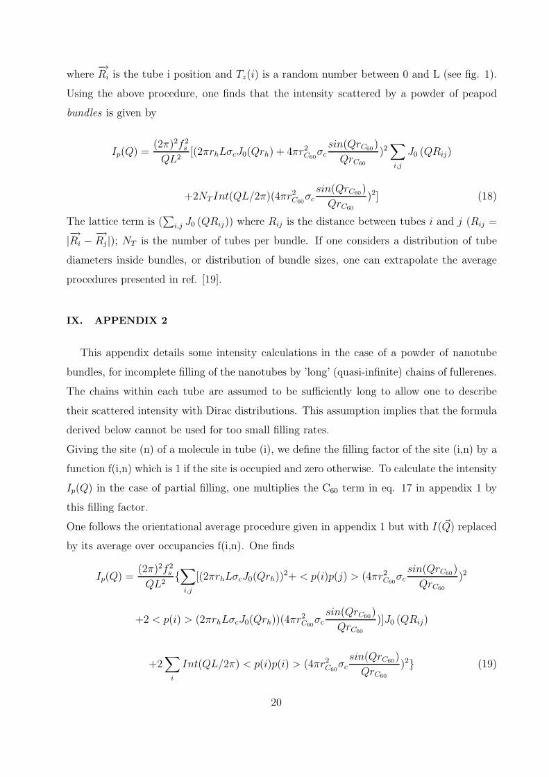
where−→Ri is the tube i position and Tz(i) is a random number between 0 and L (see fig. 1).

Using the above procedure, one finds that the intensity scattered by a powder of peapod

bundles is given by

Ip(Q) =(2π)2f 2

s

QL2[(2πrhLσcJ0(Qrh) + 4πr2

C60σc

sin(QrC60)

QrC60

)2∑

i,j

J0 (QRij)

+2NT Int(QL/2π)(4πr2C60

σcsin(QrC60)

QrC60

)2] (18)

The lattice term is (∑

i,j J0 (QRij)) where Rij is the distance between tubes i and j (Rij =

|−→Ri −

−→Rj |); NT is the number of tubes per bundle. If one considers a distribution of tube

diameters inside bundles, or distribution of bundle sizes, one can extrapolate the average

procedures presented in ref. [19].

IX. APPENDIX 2

This appendix details some intensity calculations in the case of a powder of nanotube

bundles, for incomplete filling of the nanotubes by ’long’ (quasi-infinite) chains of fullerenes.

The chains within each tube are assumed to be sufficiently long to allow one to describe

their scattered intensity with Dirac distributions. This assumption implies that the formula

derived below cannot be used for too small filling rates.

Giving the site (n) of a molecule in tube (i), we define the filling factor of the site (i,n) by a

function f(i,n) which is 1 if the site is occupied and zero otherwise. To calculate the intensity

Ip(Q) in the case of partial filling, one multiplies the C60 term in eq. 17 in appendix 1 by

this filling factor.

One follows the orientational average procedure given in appendix 1 but with I( ~Q) replaced

by its average over occupancies f(i,n). One finds

Ip(Q) =(2π)2f 2

s

QL2{∑

i,j

[(2πrhLσcJ0(Qrh))2+ < p(i)p(j) > (4πr2

C60σc

sin(QrC60)

QrC60

)2

+2 < p(i) > (2πrhLσcJ0(Qrh))(4πr2C60

σcsin(QrC60)

QrC60

)]J0 (QRij)

+2∑

i

Int(QL/2π) < p(i)p(i) > (4πr2C60

σcsin(QrC60)

QrC60

)2} (19)

20

During the course of the calculation terms containing < p(i)p(j) > arise, where p(i) is

the filling factor of tube i : p(i) = 1Nc(i)

∑Nc(i)n=1 f(i, n) where Nc(i) is the number of C60 sites

in tube i.

The filling rate of the sample, called < p > or p, is the double average of f(i, n):

< p >=1

NT Nc

NT∑

i=1

Nc∑

n=1

f(i, n) (20)

where the number of C60 sites has been taken to be the same for all tubes Nc(i) = Nc.

Three cases are considered.

(i)Homogeneous partial filling of the tubes with long chains of C60, all tubes having the same

mean filling rate p, independent of i : p(i) = p, independent of i.

In that case, equation 19 becomes :

Ip(Q) =(2π)2f 2

s

QL2[(2πrhLσcJ0(Qrh) + p4πr2

C60σc

sin(QrC60)

QrC60

)2∑

i,j

J0 (QRij)

+2NT Int(QL/2π)(p4πr2C60

σcsin(QrC60)

QrC60

)2] (21)

The C60 form factor -4πr2C60

σcsin(QrC60

)

QrC60- is multiplied by the mean filling rate p. There is

no other modification of equation 18 because one assumes that the C60 molecules agglomerate

within nanotubes to form long chains.

(ii)Partial filling of the tubes with long chains of C60 molecules, with filling rates different

from one tube to another within each bundle. In that case, one has to consider that

< p(i)p(j) >=< p2 > if i = j

< p(i)p(j) >=< p >2 if i 6= j (no correlation from one tube to another). So that

< p2 > − < p >2 6= 0.

For instance, one can consider within each bundle average proportions p of fully filled

tubes and (1-p) of empty tubes (which can be due to the fact that p% of the tubes are

opened and (1-p)% are closed), which gives: < p(i) >=p and < p(i)p(i) >=p, then

< p(i)2 > − < p(i) >2= p(1 − p) 6= 0.

The different fillings of nanotubes induce additional disorder in direct space, which corre-

sponds to diffuse scattering in reciprocal space. The additional scattering is the most intense

21

at small Q values as in the case of chemical disorder [22]. This approach is detailed in ref.[32]

for partial filling of zeolite channels with nanotubes. Eq. 18 becomes

Ip(Q) =(2π)2f 2

s

QL2[(2πrhLσcJ0(Qrh)+ < p > 4πr2

C60σc

sin(QrC60)

QrC60

)2∑

i,j

J0 (QRij)

+NT (< p2 > − < p >2)(4πr2C60

σcsin(QrC60)

QrC60

)2+2NT Int(QL/2π) < p2 > (4πr2C60

σcsin(QrC60)

QrC60

)2]

(22)

(iii) Nanotubes in the same bundle are all filled or all empty, p% of the bundles corre-

sponding to filled tubes and (1-p)% to empty ones. The scattered intensity is the sum of the

intensities for p fully filled bundles and for (1-p) empty bundles. Equation 18 becomes :

Ip(Q) = p(2π)2f 2

s

QL2[(2πrhLσcJ0(Qrh) + 4πr2

C60σc

sin(QrC60)

QrC60

)2∑

i,j

J0(QRij)

+2NT Int(QL/2π)(4πr2C60

σcsin(QrC60)

QrC60

)2]+(1−p)(2π)2f 2

s

QL2[(2πrhLσcJ0(Qrh))

2∑

i,j

J0(QRij)]

(23)

X. APPENDIX 3

This appendix details calculations in the case of polymerized C60 molecules inside the

tubes. The chains within the tubes are assumed to be formed of n-polymers of C60 molecules.

The distance between bonded C60 molecules within a n-polymer is Lb , which is smaller than

the distance L between C60 neighbors belonging to different n-polymers. For instance, for

n=2, one considers a chain of dimers and for n=3 a chain of trimers.

The form factor of a n-polymer of C60 molecules writes

Fn−polymer = 4πr2C60

σcsin(QrC60)

QrC60

(

n−1∑

k=0

eiQz(k− (n−1)2

)Lb

)

= 4πr2C60

σcsin(QrC60)

QrC60

(

e−iQz(n−1)

2Lb

1 − eiQznLb

1 − eiQzLb

)

= 4πr2C60

σcsin(QrC60)

QrC60

sin(QznLb

2)

sin(QzLb

2)

where (k- (n−1)2

)Lb is the position of the C60 molecule indexed by k within the n-polymer.

22

By replacing in eq. 15 the monomer form factor by that of the n-polymer and the period

L along the monomer chain by the one along the n-polymer chain, which is (L+(n-1)Lb),

one obtains:

I( ~Q) ∝ f 2s [(2πrh(L + (n − 1)Lb)σcJ0(Qrh)

sin(Qz(L+(n−1)Lb)/2)Qz(L+(n−1)Lb)/2

+

4πr2C60

σcsin(QrC60

)

QrC60

sin(Qz

nLb

2)

sin(Qz

Lb

2))2δ(Qz)

+(4πr2C60

σcsin(QrC60)

QrC60

sin(QznLb

2)

sin(QzLb

2)

)2∑

k 6=0

δ(Qz − 2πk/(L + (n − 1)Lb))]

Powder average thus gives :

Ip(Q) ∝ f 2s [

1

Q(2πrh(L + (n − 1)Lb)σcJ0(Qrh) + 4πr2

C60σcn

sin(QrC60)

QrC60

)2

+2

Q(1 − δN,0)

M∑

k=1

(4πr2C60

σcsin(QrC60)

QrC60

sin(πknLb/(L + (n − 1)Lb))

sin(πkLb/(L + (n − 1)Lb)))2)]

where M is the integer part of (Q(L+(n−1)L

b

2π); the term (1− δM,0) was introduced to avoid

the case M=0.

[1] : S. Iijima, Nature 354 (1991) 56

[2] : R.S. Lee, H.J. Kim, J.E. Fischer, A. Thess, R.E. Smalley, Nature 388 (1997) 255

[3] : A.M. Rao, P.C. Eklund, S. Bandow, A. Thess, R.E. Smalley, Nature 388 (1997) 257

[4] : N. Bendiab, A. Righi, E. Anglaret, J.L Sauvajol, L. Duclaux, F. Beguin, Phys. Rev. B 63

(2001) 153407

[5] : M.R. Johnson, S. Rols, P.Wass, M. Muris, M. Bienfait, P. Zeppenfeld, N. Dupont-Pavlovsky,

Chemical Physics 293 (2003) 217

[6] : B.W. Smith, M. Monthioux, D.E. Luzzi, Nature 396 (1998) 323

[7] : D.H. Kim, H.S. Sim and K.J. Chang, Phys. Rev. B 64 (2001) 115409

[8] : A. Rochefort, Phys. Rev. B 67 (2003) 115401

[9] : D.J. Hornbaker, S.J. Kahng, S. Misra, B.W. Smith, A.T. Johnson, E.J. Mele, D.E. Luzzi,

A. Yazdani, Science 295 (2002) 828

[10] : J. Vavro, M.C. Llaguno, B.C. Satishkumar, D.E. Luzzi and J.E. Fischer, Appl. Phys. Lett.

80 (2002) 1450

23

[11] : H. Kataura, Y. Maniwa, T. Kodama, K. Kikuchi, H. Hirahara, K. Suenaga, S. Iijima, S.

Suzuki, Y. Achiba and W. Kratschmer, Synthetic Metals 121 (2001) 1195

[12] : X. Liu, T. Pichler, M. Knupfer, M.S. Golden, J. Fink, H. Kataura, Y. Achiba, K. Hirahara

and S. Iijima, Phys. Rev. B 65 (2002) 045419

[13] : K. Hirahara, S. Bandow, K. Suenaga, H. Kato, T. Okazaki, H. Shinohara and S. Iijima,

Phys. Rev. B 64 (2001) 115420

[14] : H. Kuzmany, R. Pfeiffer, C. Kramberger, T. Pichler, X. Liu, M. Knupfer, J. Fink, H.

Kataura, Y. Achiba, B.W. Smith and D.E. Luzzi, Appl. Phys. A 76 (2003) 449

[15] : H. Kataura, Y. Maniwa, M. Abe, A. Fujiwara, T. Kodama, K. Kikuchi, H. Imahori, Y.

Misaki, S. Suzuki, Y. Achiba, Applied Physics A, 74 (2002) 349

[16] : Y. Maniwa, H. Kataura, M. Abe, A. Fujiwara, R. Fujiwara, H. Kira, H. Tou, S. Suzuki; Y.

Achiba, E. Nishibori, M. Takata, M. Sakata and H. Suematsu, J. of Phys. Soc. of Japan 72

(2003) 45

[17] : W. Zhou, K. I. Winey, J. E. Fischer, T. V. Sreekumar, S. Kumar, and H. Kataura, Appl.

Phys. Lett. 84 (2004) 2172

[18] : A. Thess, R. Lee, P. Nikolaev, H. Dai, P. Petit, J. Robert, C. Xu, Y.H. Lee, S.G. Kim, D.T.

Colbert, G.E. Scuseria, D. Tomanek, J.E. Fischer, R.E. Smalley, Science 273 (1996) 483

[19] : S. Rols, R. Almairac, L. Henrard, E. Anglaret, J.L. Sauvajol, The European Physical Journal

B, 10 (1999) 263

[20] : E. Anglaret, S. Rols and J.-L. Sauvajol, Phys. Rev. Lett. 81 (1998) 4780

[21] : N. Bendiab, R. Almairac, S. Rols, R. Aznar, J-L. Sauvajol, I. Mirebeau, Phys. Rev. B 69

(2004) 195415

[22] : A. Guinier, X-ray Diffraction in Crystals, Imperfect Crystals and Amorphous Bodies (Dover

Publications, 1994)

[23] : S.W. Lovesey, Theory of Neutron Scattering from Condensed Matter (Oxford Science 1984)

[24] The maximum of the asymmetric peak originating from the C60 chains is situated at Q=2π/L

= 0.66 A−1 for infinite chains. For finite chains, it becomes less abrupt and its maximum shifts

to higher Q values (namely, 0.68 A−1 for chains of 40 molecules in figure 3).

[25] : Y. Maniwa, Y. Kumazawa, Y. Saito, H. Tou, H. Kataura, H. Ishii, S. Suzuki, Y. Achiba, A.

Fujiwara, H. Suematsu , Japanese Journal of Applied Physics 38 (1999) L668

[26] The compensation leads to a zero value of the intensity for peapods of infinite lengths, and to

24

values close to zero for finite lengths.

[27] : B. Sundqvist, Adv. Phys. 48 (1999) 1

[28] : L. Forro and L. Mihaly, Rep. Prog. Phys. 64 (2001) 649

[29] : T. Pichler, H. Kuzmany, H. Kataura and Y. Achiba, Phys. Rev. Lett. 87 (2001) 267401

[30] : L. Henrard, A. Loiseau, C. Journet, and P. Bernier, Eur. Phys. J. B 13 (2000) 661

[31] : A. Fujiwara, K. Ishii, H. Suematsu, H. Kataura, Y. Maniwa, S. Suzuki and Y. Achiba,

Chem. Phys. Lett. 336 (2001) 205

[32] : P. Launois, R. Moret, D. Le Bolloc’h, P.A. Albouy, Z.K. Tang, G. Li and J. Chen, Solid

State Comm.116 (2000) 99

25

FIG. 1: Schematic representation of the system of coordinates and variables used in the calculations.

FIG. 2: Calculations of the intensity diffracted by several powders. a) nanotube of radius r=6.8

A and of length 380 A. b) linear chain of 40 C60 molecules. c) peapod (plain line), sum of the

intensities from a) and b) (dotted line), and crossed term (dashed line).

FIG. 3: Upper part of the figure : calculated powder diffraction patterns of peapods for different

tube radii : 5.42 A (8,8), 6.8 A (10,10), 8.1 A (12,12) , with an inter-C60 distance L equal to 9.5

A. Lower part of the figure : calculated diffraction patterns for different inter-C60 distances L and

for a r=6.8 A tube.

FIG. 4: Calculated diffracted intensities of a powder of isolated nanotubes (rh=6.8 A). Up: for

random filling by the C60 molecules (tube length is 380 A); down : for incomplete filling by long

(’infinite’) C60 chains. Filling rates indicated in the figure are the same for all tubes in each case

considered.

FIG. 5: Component of the calculated diffracted intensities relative to periodicity effects (only the

second term of eq. 11 is drawn) of a powder of isolated nanotubes (rh=6.8 A), for C60 monomers

(upper line), dimers (middle line) and trimers (lower line) chains inside the tubes.

FIG. 6: Comparison between the calculated intensities scattered by a powder of bundles of 12

empty nanotubes (upper curve of each part) and bundles of 12 peapods (lower curve of each part)

for (10,10) nanotubes (upper part) of radius r=6.8 A, (8,8) nanotubes (middle part) of radius

r=5.42 A and (12,12) nanotubes (lower part) of radius r=8.1 A. The tube length was fixed at 380

A in all the calculations. The arrows in the upper part point toward assymetric peaks characteristic

of the 1D periodicity of C60 chains.

26

FIG. 7: Left top : Diffraction patterns of 85% filled bundles of 12 peapods. Left bottom : Diffraction

patterns of 50% filled bundles of 12 peapods. All tubes have a radius of 6.8 A. Right part : Schematic

representations of the 4 different filling modes used in calculations : a) random positions for the

C60 molecules within each tube, same filling for each tube, b) long C60 chains, same filling for each

tube , c) long C60 chains, inhomogeneous filling of the different tubes within a bundle, d) mix of

full and empty bundles.

FIG. 8: Effect on diffraction pattern of the filling of the external channels with C60s linear chains

for different sizes of bundles. All tubes have a radius of 6.8 A and are 380 A long. a) 4 tubes. b)

6 tubes compared with a 6 tubes naked bundle (dotted line). c) 12 tubes.

FIG. 9: Filling rate determination. a) First criterium giving the amplitude ratio

I(.663A−1)/I(.706A−1) as function of the filling rate p (see the inset), calculated for randomly

filled (empty circles) and homogeneously filled (full circles) bundles of peapods. b) Second cri-

terium: amplitude ratio of the peaks around 1.3 A−1 and 1.1 A−1 as function of p (see the inset),

calculated for randomly filled (empty circles), inhomogeneously filled (empty triangles) and homo-

geneously filled (full circles) bundes of peapods. The dashed and dotted horizontal lines represent

the experimental finding for the two investigated samples A and B.

FIG. 10: Experimental diffraction patterns of peapod samples. a) Peapod sample A (upper line),

corresponding MER pristine SWNT sample (lower line). The dotted line is the baseline used for

the fits. b) Peapods sample B (upper line) and a calculation of its diffraction profile (lower line).

27