On the Data Gathering Capacity and Latency inWireless Sensor Networks

Paolo Santi, Member, IEEE,IIT-CNR

Pisa, ITALY

Abstract—In this paper, we investigate the fundamental prop-erties of data gathering in wireless sensor networks, in terms ofboth capacity and latency. We consider a scenario in which s(n)out of n total network nodes have to deliver data to a set ofd(n) sink nodes at a constant rate λ(n, s(n), d(n)). The goal isto characterize the maximum achievable rate, and the latencyin data delivery. We present a simple data gathering schemethat achieves asymptotically optimal data gathering capacity andlatency with arbitrary network deployments when d(n) = 1, andfor most scaling regimes of s(n) and d(n) when d(n) > 1 incase of square grid and random node deployments. Differentlyfrom most previous work, our results and the presented datagathering scheme do not sacrifice energy efficiency to the need ofmaximizing capacity and minimizing latency. Finally, we considerthe effects of a simple form of data aggregation on data gatheringperformance, and show that capacity can be increased by afactor f(n) with respect to the case of no data aggregation,where f(n) is the node density. To the best of our knowledge,the ones presented in this paper are the first results showing thatasymptotically optimal data gathering capacity and latency can beachieved in arbitrary networks in an energy efficient way.

Index terms: Wireless sensor networks, data gathering ca-pacity, data gathering latency, physical interference model.

I. INTRODUCTION

After several years of intensive research and technologicaldevelopment, wireless sensor networks are becoming increas-ingly deployed in a wide range of application scenarios, andwill likely be part of our everyday life in a few years. Despitethat, our understanding of fundamental properties of thesenetworks – the so-called scaling laws –, which can help thenetwork designer discriminating what can and cannot be donein such networks, is still limited. In particular, network capac-ity and communication latency are two fundamental propertiesof a wireless sensor network: the former can help charac-terizing the overall amount of data that can be transportedwithin the network, while the latter can help understanding,for instance, whether the network can be effectively used forreal-time event detection. When a wireless sensor network isto be used for, e.g., environmental monitoring, in which anextensive set of sensor readings has to be collected at one orfew data collection sites (sinks), the combined characterizationof network capacity and communication latency scaling lawsis fundamental to understanding feasibility of a large scalenetwork deployment.

Starting from the seminal Gupta and Kumar’s work oncapacity [7] for unicast transmissions, fundamental propertiesof general wireless multihop networks have been extensivelystudied in the literature in the last few years (see Section II

for details). These studies have shown a considerable influenceof the network topology and traffic patterns on the achievablenetwork capacity and latency limits. For instance, in [7] ithas been shown that while the per-node capacity in a networkcomposed of n nodes degrades as O

(1√n

)when n grows

to infinity in arbitrary networks, it degrades at a faster pace(as O

(1√

n logn

)) if nodes are randomly deployed. The above

results hold under the assumption that traffic source/destinationpairs are randomly chosen. However, if communications arelocalized (i.e., the destination of a packet is randomly chosenamongst one of the source’s immediate neighbors), the situa-tion is drastically different, and per-node throughput actuallyremains constant as n grows to infinity. Another exampleof the influence of the traffic pattern on network capacityand communication latency can be derived by comparingthe findings of [13], which show that asymptotically optimalcapacity and latency cannot be simultaneously achieved forunicast transmissions, with those of [15], which show thatasymptotically optimal capacity and latency can indeed besimultaneously achieved for broadcast communications.

Given the above discussion, it is clear that characterizing thecapacity and latency scaling laws of a wireless sensor networkrequires taking into account the typical traffic patterns of thistype of networks. In this paper, we consider one such typicalpattern – the data gathering pattern –, in which many (or all)the sensor nodes have to regularly deliver data to one (or few)sink node(s). The data gathering network capacity has beenrecently investigated in a few papers [4], [11], [12], [24] (seeSection II for details), which, however, are based on quite strictassumptions for what concerns network topology, propertiesof the observed random field, and/or PHY layer capabilities.When simultaneous transmissions are allowed in the network[11], [12], radio interference is modeled using a relativelyinaccurate interference model (the protocol interference model[7]). Furthermore, the effects of data aggregation strategieson the achievable network capacity have only be partiallyconsidered. Most importantly, none of the existing works isconcerned with energy efficiency of the communications, norconsiders latency in data communication. There is no need tocomment on the importance of energy efficient communicationin wireless sensor networks. As for latency, we stress thatlatency is a fundamental property in many wireless sensornetwork application scenarios, for instance when the networkis used for real-time event detection.

The main findings of this paper, which are extensively

2

described at the end of Section II, are that asymptoticallyoptimal data gathering capacity and latency can be simultane-ously achieved in arbitrary and random networks in an energyefficent manner, as long as the network deployment satisfiesa property which we call minimal cell connectivity. The datagathering capacity is limited by the number of sink nodes inthe network, and can thus be improved (up to a certain point)by increasing the number of data collection sites. Another wayof improving the data gathering capacity is by exploiting avery simple form of data aggregation, which increases networkcapacity of an O(f(n)) factor, where f(n) is the node density.

The rest of this paper is organized as follows. In SectionII, we discuss related work and extensively describe thispaper’s contributions to the state-of-the-art. In Section III,we introduce the network model used in the rest of thepaper. In Section IV, we consider the case of single sinknetworks, and present a data gathering scheme that providesasymptotically optimal data gathering capacity and latency. InSection V, we extend the data gathering scheme to the caseof multiple sink networks, and characterize conditions underwhich asymptotically optimal data gathering capacity can beachieved. Section VI discusses energy efficiency of the datagathering schemes proposed in sections IV and V. Finally,Section VII summarizes the main results of the paper anddiscuss their implications for the design of wireless sensornetwork data gathering applications.

II. RELATED WORK AND CONTRIBUTIONS

The investigation of fundamental wireless network proper-ties has been subject of intensive research since the seminalGupta and Kumar’s work [7]. In [7], the authors lay downthe foundations of wireless multihop networking, showing thatshort-range communications have to be preferred to long-rangecommunications if the objective is to maximize network ca-pacity. This is due to the fact that short-range communicationsminimize the interference level in the network, allowing for adegree of spatial reuse (i.e., simultaneous transmissions) thatis sufficient to outweigh the relay burden caused by multi-hop communications. However, this relay burden considerablylimits per-node network capacity, which is shown to convergeto 0 as the number n of network nodes grows to infinity. In[6], Grossglauser and Tse show that the Gupta and Kumar’scapacity limit does not apply in mobile networks: the mainidea is to exploit node mobility, rather than multihop forward-ing, to deliver packets to the destinations. This way, per-nodecapacity can be optimized (i.e., Ω(W ) per-node capacity canbe achieved, where W is the channel capacity), at the price ofconsiderably increasing communication latency. The tradeoffbetween network capacity and latency in packet delivery isinvestigated, e.g., in [13], [20]. In particular, in [13] the authorsshow that the achievable per-node capacity is upper boundedby O

(Dn

), where D is the average packet delay. This result

implies that Ω(W ) per-node capacity can be achieved onlyby allowing O(n) latency, which is not optimal in most two-dimensional deployment scenarios.

The above results refer to the unicast communication pat-tern. Other traffic patterns have been recently investigated,such as multicast [10], [19] and broadcast [8], [9], [15], [16],

[17], [23]. We briefly comment on the results concerningbroadcast communications, which are indeed relevant to wire-less sensor networks (think about a sink node broadcasting aquery in the network, downloading new software to the nodes,etc.). In [23], Zheng investigates the broadcast capacity ofrandom networks with single broadcast source, and presents abroadcast scheme providing asymptotically optimal capacity.The author also studies the information diffusion rate, whichis closely related to latency. However, broadcast capacityand information diffusion rate are not jointly considered, i.e.,the capacity-achieving broadcast scheme does not optimizediffusion rate, and vice-versa. In [8], [9], the authors consider amore general network model, in which arbitrary node positionsand arbitrary number of broadcast sources are allowed. Theresults of [8], [9] essentially confirm the finding on broadcastcapacity reported in [23] in the more general model. In[15], the authors consider a network model similar to thatof [9] (but assuming a single broadcast source), and showthat asymptotically optimal broadcast capacity and latency canbe achieved, subject to a (not very restrictive) condition onnetwork topology. This result has been recently generalizedto the case of arbitrary number of sources in [16], and to thecase of mobile nodes [17].

The data gathering capacity of wireless networks has beeninvestigated in a few recent papers. In [12], the authorsconsider a model in which nodes are evenly spaced in acircular area. Nodes monitor a random, spatially-correlatedfield, and the goal is to deliver snapshots of this random fieldto a sink, located in the center of the area. As the node densityincreases, correlation of the sensed data increases, as well asthe demand of traffic directed to the sink. Since correlateddata can be compressed, the question addressed in [12] iswhether data compression can be exploited to deliver accuratesnapshots of the random field (with an upper bounded MSE)to the sink. The authors essentially prove a negative result,showing that the benefits of data compression are not sufficientto outweigh the capacity bottleneck at the sink node, whichimplies that the per-source available capacity is O

(Wn

). In [4],

El Gamal shows how to go beyond this per-node capacity limitachieving O

(W logn

n

)per-source capacity, which is proved

to be sufficient to guarantee delivery of accurate snapshotsof a Gaussian, bandwidth-limited random field. The mainidea to improve capacity is exploiting advanced PHY layertechniques, namely cooperative communication: every nodedistributes its sampled value to neighboring nodes, and thenall these nodes cooperatively transmit the information to thesink node, realizing distributed beamforming. Thus, owingto the beamforming gain, capacity at the sink node can beincreased of a logarithmic factor. Although interesting from atheoretical point of view, El Gamal’s result is hard to apply ina practical scenario, due to the many assumptions on whichit is based: nodes are evenly spaced on a sphere, with thesink node located in the center of the sphere; at the PHYlayer, nodes are assumed to perform transmit power control,to know the radio signal phase shifts between all possible pairsof nodes, to be able to perform cooperative communication,etc.; finally, the joint distribution of the random field observed

3

at the various nodes is assumed to be known to all sensornodes. More recently, Zheng and Barton [24] have shown thebenefits of cooperative communication in a less constrainedenvironment, where nodes are randomly distributed, use acommon transmit power, and a-priori statistical knowledge ofthe observed random field and of the channel characteristicsare not needed. In particular, the authors show that even inthis less constrained environment O

(W logn

n

)data gathering

capacity can be achieved as long as path loss exponent αis such that 2 < α < 4; indeed, for these values of αthe achieved capacity is shown to match the asymptoticalupper bound, i.e., it is shown to be optimal. If α > 4, theupper bound to capacity becomes O(Wn ), and optimal capacitycan be achieved even without cooperative communication.Notice that although Zheng and Barton’s results are based onless demanding assumptions than [3], they still build uponexploitation of advanced PHY layer techniques (cooperativecommunication), that might be difficult to use in a wirelesssensor network.

The work that is more closely related to ours is [11],in which the authors investigate the data gathering capacityof a randomly deployed network in which s(n) out of then nodes act as data sources, d(n) nodes are data sinks,and each source node is randomly mapped to a sink node.In this model, the authors identify two different asymptoticregimes: if d(n) = O

(√n

logn

), performance is constrained

by the aggregate sink reception capacity, and per-source ca-pacity is upper bounded by O

(W ·d(n)s(n)

); if d(n)

√n

logn ,performance is constrained by network capacity, and per-

source capacity saturates to O

(W ·√n/ logn

s(n)

)independently

of the number d(n) of sink nodes. The authors also presenta scheduling/routing algorithm to constructively lower boundcapacity, and prove that the proposed construction indeedachieves asymptotically optimal data gathering capacity formost scaling regimes of s(n) and d(n).

In this paper, we consider a traffic model similar to [11],in which s(n) nodes are data sources and d(n) nodes aredata sinks. However, differently from [11], we assume thatsource/sink mapping obeys a locality criterion. In this model,we provide the following contributions:a) for the first time, we analyze not only data gathering

capacity, but also latency. In particular, in some cases (seebelow) we present data gathering schemes simultaneouslyachieving asymptotical capacity and latency. We stressthat turning a capacity achieving data gathering schemeinto one that optimizes both capacity and latency is nota trivial task (see the construction used in Section IV).

b) for the many-to-one case (i.e., d(n) = 1), we presenta data gathering scheme that achieves asymptoticallyoptimal data gathering capacity for arbitrary networkdeployments. To the best of our knowledge, ours isthe first capacity-achieving construction for arbitrarynetwork deployments. Furthermore, we show that, if acertain topological property that we call minimal cellconnectivity is satisfied, the presented scheme achievesnot only asymptotically optimal capacity, but also asymp-

totically optimal latency in data gathering.c) for the many-to-many case with arbitrary s(n) and d(n),

we consider both square grid and random network de-ployments, and present an extension of the data gatheringscheme for single source networks that achieves asymp-totically optimal data gathering latency. Furthermore, formost scaling regimes of s(n) and d(n), the presentedconstruction achieves also asymptotically optimal per-source data gathering capacity. In particular, the resultsfor random network deployments show that per-sourcecapacity can exceed the bounds established in [11] when√

nlogn d(n) = O

(n

logn

). This is due to the different

rule used to map data source to sinks: random in [11],locality-based in our study.

c) finally, we consider the effect of a simple form of dataaggregation based on a notion of sensing granularity, andshow that per-source capacity can be increased by a factorf(n) with respect to the case of no data aggregation whilepreserving asymptotically optimal latency, where f(n) isnode density.

Notably, and differently from most previous works, thepresented results and data gathering scheme do not sacrificeenergy efficiency to the need of maximizing capacity andminimizing latency. Furthermore, we want to stress that,differently from previous work on data gathering capacity, theresults in this paper are derived using an accurate, SINR-basedinterference model, the physical interference model of [7].

III. NETWORK MODEL AND PRELIMINARIES

We consider a wireless sensor network composed of nnodes, where s(n) ≤ n − 1 nodes act as data sources,d(n) ≤ n − s(n) nodes act as data collection points (sinks),and the remaining n−s(n)−d(n) nodes may be used to relaydata to the sinks. When multiple sink nodes are present in thenetwork, the mapping between data sources and sinks obeysa locality criterion, which will be detailed in the following.

We assume nodes communicate through a common wirelesschannel of a certain, constant capacity W , and that thenodes transmission power is fixed to some constant value P .Correctness of packet reception is governed by a condition onSINR, according to the so-called physical interference model[7]. More specifically, when a node u transmits a packet toanother node v, the packet is correctly received (at constantrate W ) if and only if

SINR(v) =Pv(u)

N +∑i∈T Pv(i)

≥ β ,

where N is the background noise, β > 0 is the capturethreshold, T is the set of nodes transmitting concurrently withnode u, and Pv(x) is the received power at node v of the signaltransmitted by node x. We make the standard assumptionthat radio signal propagation obeys the log-distance path lossmodel, according to which the received signal strength atdistance d from the transmitter (for sufficiently large d, say,d ≥ 1) equals P · d−α, where α is the path loss exponent. Inthe following, we make the standard assumption that α > 2,which is often the case in practice. Up to tedious technicaldetails, our results can be generalized to the cost-based radio

4

u

v

P P’

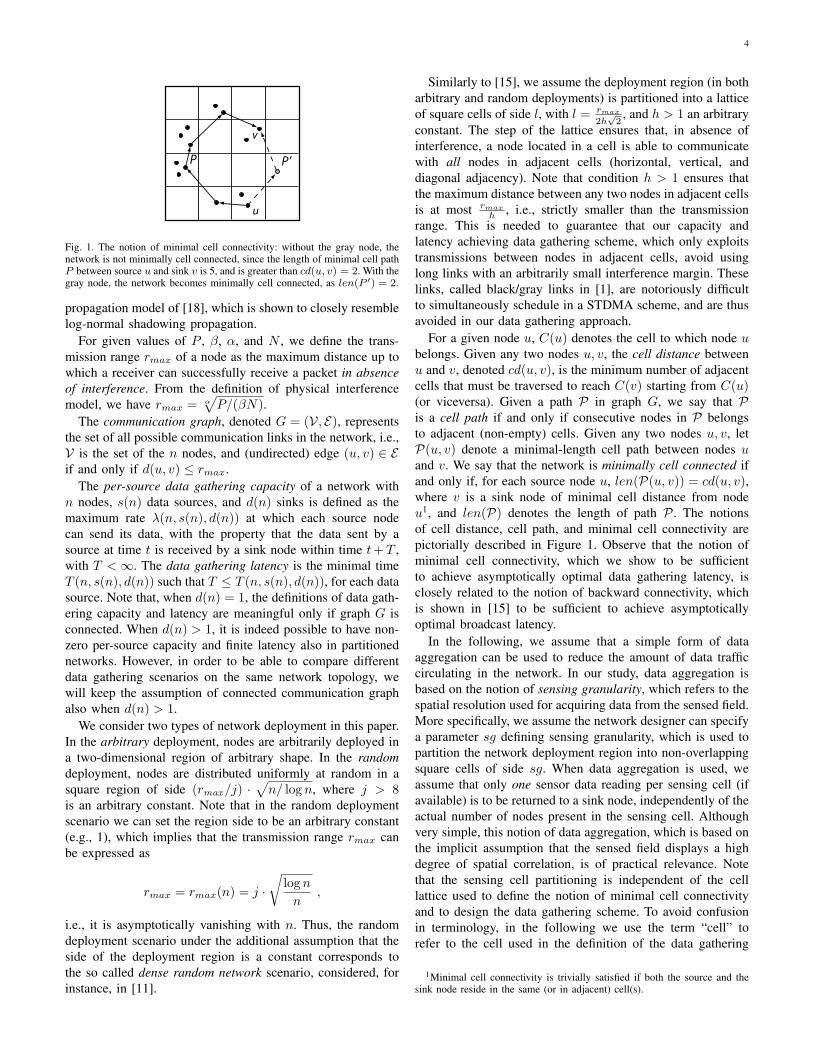
Fig. 1. The notion of minimal cell connectivity: without the gray node, thenetwork is not minimally cell connected, since the length of minimal cell pathP between source u and sink v is 5, and is greater than cd(u, v) = 2. With thegray node, the network becomes minimally cell connected, as len(P ′) = 2.

propagation model of [18], which is shown to closely resemblelog-normal shadowing propagation.

For given values of P , β, α, and N , we define the trans-mission range rmax of a node as the maximum distance up towhich a receiver can successfully receive a packet in absenceof interference. From the definition of physical interferencemodel, we have rmax = α

√P/(βN).

The communication graph, denoted G = (V, E), representsthe set of all possible communication links in the network, i.e.,V is the set of the n nodes, and (undirected) edge (u, v) ∈ Eif and only if d(u, v) ≤ rmax.

The per-source data gathering capacity of a network withn nodes, s(n) data sources, and d(n) sinks is defined as themaximum rate λ(n, s(n), d(n)) at which each source nodecan send its data, with the property that the data sent by asource at time t is received by a sink node within time t+T ,with T <∞. The data gathering latency is the minimal timeT (n, s(n), d(n)) such that T ≤ T (n, s(n), d(n)), for each datasource. Note that, when d(n) = 1, the definitions of data gath-ering capacity and latency are meaningful only if graph G isconnected. When d(n) > 1, it is indeed possible to have non-zero per-source capacity and finite latency also in partitionednetworks. However, in order to be able to compare differentdata gathering scenarios on the same network topology, wewill keep the assumption of connected communication graphalso when d(n) > 1.

We consider two types of network deployment in this paper.In the arbitrary deployment, nodes are arbitrarily deployed ina two-dimensional region of arbitrary shape. In the randomdeployment, nodes are distributed uniformly at random in asquare region of side (rmax/j) ·

√n/ log n, where j > 8

is an arbitrary constant. Note that in the random deploymentscenario we can set the region side to be an arbitrary constant(e.g., 1), which implies that the transmission range rmax canbe expressed as

rmax = rmax(n) = j ·√

log nn

,

i.e., it is asymptotically vanishing with n. Thus, the randomdeployment scenario under the additional assumption that theside of the deployment region is a constant corresponds tothe so called dense random network scenario, considered, forinstance, in [11].

Similarly to [15], we assume the deployment region (in botharbitrary and random deployments) is partitioned into a latticeof square cells of side l, with l = rmax

2h√

2, and h > 1 an arbitrary

constant. The step of the lattice ensures that, in absence ofinterference, a node located in a cell is able to communicatewith all nodes in adjacent cells (horizontal, vertical, anddiagonal adjacency). Note that condition h > 1 ensures thatthe maximum distance between any two nodes in adjacent cellsis at most rmax

h , i.e., strictly smaller than the transmissionrange. This is needed to guarantee that our capacity andlatency achieving data gathering scheme, which only exploitstransmissions between nodes in adjacent cells, avoid usinglong links with an arbitrarily small interference margin. Theselinks, called black/gray links in [1], are notoriously difficultto simultaneously schedule in a STDMA scheme, and are thusavoided in our data gathering approach.

For a given node u, C(u) denotes the cell to which node ubelongs. Given any two nodes u, v, the cell distance betweenu and v, denoted cd(u, v), is the minimum number of adjacentcells that must be traversed to reach C(v) starting from C(u)(or viceversa). Given a path P in graph G, we say that Pis a cell path if and only if consecutive nodes in P belongsto adjacent (non-empty) cells. Given any two nodes u, v, letP(u, v) denote a minimal-length cell path between nodes uand v. We say that the network is minimally cell connected ifand only if, for each source node u, len(P(u, v)) = cd(u, v),where v is a sink node of minimal cell distance from nodeu1, and len(P) denotes the length of path P . The notionsof cell distance, cell path, and minimal cell connectivity arepictorially described in Figure 1. Observe that the notion ofminimal cell connectivity, which we show to be sufficientto achieve asymptotically optimal data gathering latency, isclosely related to the notion of backward connectivity, whichis shown in [15] to be sufficient to achieve asymptoticallyoptimal broadcast latency.

In the following, we assume that a simple form of dataaggregation can be used to reduce the amount of data trafficcirculating in the network. In our study, data aggregation isbased on the notion of sensing granularity, which refers to thespatial resolution used for acquiring data from the sensed field.More specifically, we assume the network designer can specifya parameter sg defining sensing granularity, which is used topartition the network deployment region into non-overlappingsquare cells of side sg. When data aggregation is used, weassume that only one sensor data reading per sensing cell (ifavailable) is to be returned to a sink node, independently of theactual number of nodes present in the sensing cell. Althoughvery simple, this notion of data aggregation, which is based onthe implicit assumption that the sensed field displays a highdegree of spatial correlation, is of practical relevance. Notethat the sensing cell partitioning is independent of the celllattice used to define the notion of minimal cell connectivityand to design the data gathering scheme. To avoid confusionin terminology, in the following we use the term “cell” torefer to the cell used in the definition of the data gathering

1Minimal cell connectivity is trivially satisfied if both the source and thesink node reside in the same (or in adjacent) cell(s).

5

scheme, and the term “sensing cell” to refer to the cell usedto aggregate data to be delivered to the sink(s).

We conclude this section with two known properties ofthe random network deployment, which will be useful in theremainder of this paper.

Proposition 1. (from [5]) In the dense random deploymentscenario, the critical transmission range for connectivity2 is:

ctr(n) =rmax(n)

j.

Proposition 2. (from [15]) In the random deployment sce-nario, let Cmin denote the number of nodes in the minimallyoccupied cell in the lattice. We have Prob(Cmin > 0)→ 1 asn → ∞, i.e., w.h.p., each cell in the lattice contains at leastone node.

A straightforward consequence of Proposition 2 is that arandomly deployed network satisfies minimal cell connectivity,w.h.p.

IV. SINGLE SINK NETWORKS

A. No data aggregation

We first consider the case of single sink networks, i.e.,throughout this section we assume d(n) = 1. Differently frommost existing works on data gathering capacity, our resultshold independently of the location of the sink node within thenetwork.

We start by stating the upper bounds on data gatheringcapacity and latency, which hold for both arbitrary and randomnetwork deployments.

Proposition 3. The per-source data gathering capacity of asingle sink network with s(n) data sources is O

(Ws(n)

), where

W is the capacity of the wireless link. The data gatheringlatency is Ω

(D(n)rmax

), where D(n) is the network diameter.

The upper bound on capacity follows by observing, simi-larly to [11], [12], that the sink node can receive data from atmost one node at any instant of time, that the channel data rateis W , and that sink reception capacity must be shared amongsts(n) sources. We thus do not consider use of advanced PHYlayer techniques to exceed the O(W ) receiving capacity limitat the sink node, as proposed in [4], [24]. The lower boundon latency is based on the observation that, under our networkmodel, a packet can travel at most distance rmax towards thesink node at each communication round.

We now present the capacity and latency achieving datagathering scheme. We assume that each node v is aware ofthe cell C(v) to which it belongs, and that a spatial TDMAapproach is used at the MAC layer. Furthermore, we assumethat cells are colored according to a two-dimensional coloringscheme (see Figure 2), similar to those used, e.g., in [8],[15]. More specifically, the color of a cell (and of all thenodes belonging to that cell) is a tuple (i, j), with i thehorizontal color and j the vertical color. A total of k2 colors,

2The critical transmission range for connectivity is defined as the minimumvalue of the transmission range such that the resulting communication graphis connected with high probability, i.e., with probability approaching 1 as ngrows to infinity.

(2 , 0)

(2 , 1)

(2 , 2)

(2 , 0)

(2 , 1)

(2 , 2)

(2 , 0)

(0 , 0)

(0 , 1)

(0 , 2)

(0 , 0)

(0 , 1)

(0 , 2)

(0 , 0)

(1 , 0)

(1 , 1)

(1 , 2)

(1 , 0)

(1 , 1)

(1 , 2)

(1 , 0)

(2 , 0)

(2 , 1)

(2 , 2)

(2 , 0)

(2 , 1)

(2 , 2)

(2 , 0)

(0 , 0)

(0 , 1)

(0 , 2)

(0 , 0)

(0 , 1)

(0 , 2)

(0 , 0)

(1 , 0)

(1 , 1)

(1 , 2)

(1 , 0)

(1 , 1)

(1 , 2)

(1 , 0)

(2 , 0)

(2 , 1)

(2 , 2)

(2 , 0)

(2 , 1)

(2 , 2)

(2 , 0)

(0 , 0)

(0 , 1)

(0 , 2)

(0 , 0)

(0 , 1)

(0 , 2)

(0 , 0)

(1 , 0)

(1 , 1)

(1 , 2)

(1 , 0)

(1 , 1)

(1 , 2)

(1 , 0)

(2 , 0)

(2 , 1)

(2 , 2)

(2 , 0)

(2 , 1)

(2 , 2)

(2 , 0)

(0 , 0)

(0 , 1)

(0 , 2)

(0 , 0)

(0 , 1)

(0 , 2)

(0 , 0)

(1 , 0)

(1 , 1)

(1 , 2)

(1 , 0)

(1 , 1)

(1 , 2)

(1 , 0)

Fig. 2. Two-dimensional coloring scheme used in the data gathering schemewith k = 3. Cells with the same color (0, 0) are shaded.

for some constant k > 0, are used, i.e., both the horizontaland vertical colors take values in 0, . . . , k−1. The coloringscheme is used in an obvious way to form the transmissionschedule, i.e., time is subdivided into slots of equal timeduration, which are numbered in a cyclical fashion between 0and k2 − 1; each color is assigned a transmission opportunityat each communication round composed of k2 consecutivetransmission slots. When the slot corresponding to color (i, j)is active, only links whose transmitter is in a cell of color(i, j) can be scheduled for transmission.

The following lemma, proved in [15], is a fundamentalbuilding block of our construction:

Lemma 1. Assume a cell partitioning as defined in SectionIII, and assume that at most one node per cell with the samecolor transmits. If

k ≥ k =⌈2 + 2

32 + 4

α (βζ(α− 1)hα/(hα − 1))1α

⌉,

where ζ is the Riemann’s zeta function, then the packet sentby a node is correctly received by all nodes in adjacent cells.

The lemma states that a constant degree of spatial separation(number of colors) is sufficient to achieve successful packetreception in neighboring cells, under the assumption that atmost one node per cell with the same color is simultaneouslytransmitting. Thus, a constant degree of spatial separation issufficient to achieve Ω(rmax) (recall that the size of the cellis Θ(rmax)) progress of a packet towards the sink (if minimalcell connectivity is satisfied).

The data gathering scheme is reported in Figure 3. De-pending on its role, each network node is classified as eithersink, source node, or relay node. The sink node is the onlydata collector in the network. Source nodes generate new datapackets to be delivered to the sink; furthermore, they can act asdata forwarders if they are not sending their own data. Relaynodes can act only as forwarders of data generated by sourcenodes. Non-sink nodes (either source or relay nodes) can beselected as leader nodes in their cell. There is a unique leadernode in each non-empty cell, which is selected according tosome rule, such as at random, remaining battery level, etc.Leader nodes act as forwarders of data towards the sink.Note that only relay nodes that are cell leaders participatein forwarding the collected data to the sink. Non-leader relaynodes actually do not take part in the data gathering scheme,and can be considered as non-active nodes (and possibly putinto sleep mode to save energy).

The data gathering scheme is very simple. Non-sink nodesare allowed to transmit only if the current slot color corre-

6

Algorithm for a generic non-sink node v:Let i be the color of the current time slotNode v has a single position packet buffer1. if color(v) = i then2. if (source(v) and MyTurn(v)) then

generate and transmit new packet3. else if cellLeader(v) then4. if buffer(v) is not empty then5. transmit packet and empty buffer6. else // color(v) 6= i7. if cellLeader(v) then8. listen to the channel9. if new packet arrive then10. receive the packet and store in transmit buffer

Algorithm for the sink node:1s. At each time slot:2s. listen to the channel3s. if new packet arrive then4s. receive the packet and deliver to user application

Fig. 3. The data gathering scheme with single sink node.

sink node source node source leader node relay leader node relay node

Fig. 4. The data gathering tree. Sensing cells are shown with dashed lines. Ifdata aggregation is used, only one source node per sensing cell is active.

sponds to the node color. If the node is a source, a furthercondition must be satisfied in order to enable transmission ofa new packet. This condition, which is verified by functionMyTurn() at step 2., ensures that data generated by thevarious sources do not conflict at intermediate nodes in theirroute to the sink. In the following, we show the constructivetechnique used to calculate function MyTurn() for eachsource node, and prove its correctness. If transmission of a newdata packet is not allowed, the node can act as forwarder ofdata generated by other sources if it is a leader node (step 3.).If the current slot color does not correspond to the node color,the node actively participates in the data gathering schemeonly if it is a leader. In this case, it checks whether a newpacket is received at the current time slot, and stores the newpacket in the buffer. The data gathering algorithm for the sinknode is straightforward.

To ensure collision-free delivery of data to the sink andoptimal latency (in case minimal cell connectivity is satisfied),data is conveyed to the sink through a cell-based shortest pathtree, called the data gathering tree, where the transmissiontime (slot) for each data source is appropriately computed3.An example of data gathering tree is reported in Figure 4: foreach source node v, a minimal length cell path to sink node

3A similar construction and transmission time computation has been usedin the broadcast scheme for arbitrary number of sources presented in [16].

1

1

1 1

21

1

11

1

3

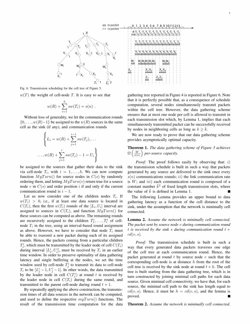
Fig. 5. The cell tree corresponding to the data gathering tree of Figure 4. Onlypositive cell-node weights are shown.

s, denoted P(v, s), is randomly selected as data forwardingpath4. Note that, without loss of generality, we can assumethat P(v, s) − v, s is composed only of leader nodes. Thecomposition of all these minimal length cell paths (one foreach source) forms the data gathering tree.

Starting from the data gathering tree, a simplified gatheringtree, called cell tree, is constructed as follows. A cell-node isassociated with each cell with at least one node in the datagathering tree. With a slight abuse of notation, in the followingwe use C(T ) to denote the cell corresponding to cell-node Tin the cell tree. An edge is present between cell-nodes T andU if and only if there is at least one edge between a node inC(T ) and a node in C(U) in the data gathering tree. Eachcell-node is assigned with a weight equal to the number ofsource nodes present in the corresponding cell. The cell treecorresponding to the data gathering tree of Figure 4 is reportedin Figure 5.

The main idea of the data gathering scheme is to have thesink node receiving a new packet from a different data sourceat each communication round. Since the communication roundis composed of a constant number k2 of transmission slots,and the total number of sources is s(n), we have that eachsource delivers packets to the sink with a rate of W

k2·s(n)=

Ω( Ws(n) ), which is asymptotically optimal. Furthermore, data

source transmission times are set in such a way that conflict atintermediate nodes of the cell tree are avoided, which ensuresthat a packet transmitted by source v during communicationround t is received by sink s at communication round t +cd(v, s). As we shall see, this property implies asymptoticallyoptimal data gathering latency when minimal cell connectivityof the network is satisfied.

The transmission time for each source node in the networkis recursively computed as follows, starting from the root ofthe cell tree, which corresponds to the cell containing thesink node. Communications rounds (each composed of k2

transmission slots) are cyclically numbered from 0 to s(n)−1.In the following, all the mathematics is modulo s(n).

Let T1, . . . , Th be the children of the root node R in the celltree, and let sw(Ti) be the sum of the weights of all cell-nodesbelonging to the subtree rooted at Ti. Furthermore, denote by

4The choice of the actual minimal length cell path used to deliver data tothe sink, which determines the tree topology, has no influence on the datagathering capacity and latency achieved by our scheme.

7

1

1

1

1

1

1

1 1

3

1

2

... 0 1 2 3 4 5 6 7 8 9 10111213 ...tx packetrx packet

T1

T2 T3T4 T5

T1 T2 T2 T2 T2 T2 T2 T2R R T3 T4 T5 T5 T5

T1

V1 V2 V3 V4

V6

T2

V1

T2 T2 T2 T2 T2 T2

V1 V2 V2 V2 V2 V2

T3

V3

T4

V4

T5 T5 T5

V5

V5 V5 V6

W1 W2 W3

W1 W2W2 W2W2W2 W3

X1X2

X3 X4

X1 X2 X3

W3

X4 X4

Z1 Z2

Z1 Z2 Z2

Fig. 6. Transmission scheduling for the cell tree of Figure 5.

w(T ) the weight of cell-node T . It is easy to see that

w(R) +h∑i=1

sw(Ti) = s(n) .

Without loss of generality, we let the communication rounds0, . . . , w(R)−1 be assigned to the w(R) sources in the samecell as the sink (if any), and communication roundsLi = w(R) +

i−1∑j=1

sw(Tj), . . .

. . . , w(R) +i∑

j=1

sw(Tj)− 1 = Ui

be assigned to the sources that gather their data to the sinkvia cell-node Ti, with i = 1, . . . , h. We can now computefunction MyTurn() for source nodes in C(s) by randomlyordering them, and letting MyTurn(v) return true for a sourcenode v in C(s) and order position i if and only if the currentcommunication round is i− 1.

Let us now consider one of the children nodes Ti. Ifw(Ti) > 0, i.e., if at least one data source is located inC(Ti), then the first w(Ti) rounds of the [Li, Ui] interval areassigned to sources in C(Ti), and function MyTurn() forthese sources can be computed as above. The remaining roundsare recursively assigned to the children T i1, . . . , T

il of cell-

node Ti in the tree, using an interval-based round assignmentas above. However, we have to consider that node Ti mustbe able to transmit a new packet during each of its assignedrounds. Hence, the packets coming from a particular childrenT ij , which must be transmitted by the leader node of cell C(Ti)during interval [Lij , U

ij ], must be received by Ti in an earlier

time window. In order to preserve optimality of data gatheringlatency and single buffering at the nodes, we set the timewindow used by cell-node T ij to transmit its data to cell-nodeTi to be [Lij − 1, U ij − 1]. In other words, the data transmittedby the leader node in cell C(T ij ) at round t is received bythe leader node in cell C(Ti) during the same round, andtransmitted to the parent cell-node during round t+ 1.

By repeatedly applying the above construction, the transmis-sion times of all data sources in the network can be computed,and used to define the respective myTurn() functions. Theresult of the transmission time computation for the data

gathering tree reported in Figure 4 is reported in Figure 6. Notethat it is perfectly possible that, as a consequence of schedulecomputation, several nodes simultaneously transmit packetswithin the cell tree. However, the data gathering schemeensures that at most one node per cell is allowed to transmit ineach transmission slot which, by Lemma 1, implies that eachsimultaneously transmitted packet can be successfully receivedby nodes in neighboring cells as long as k ≥ k.

We are now ready to prove that our data gathering schemeprovides asymptotically optimal capacity.

Theorem 1. The data gathering scheme of Figure 3 achievesΩ(Ws(n)

)per-source capacity.

Proof: The proof follows easily by observing that: i)the transmission schedule is built in such a way that packetsgenerated by any source are delivered to the sink once everys(n) communications rounds; ii) the link communication rateis W ; and iii) each communication round is composed of aconstant number k2 of fixed length transmission slots, wherethe value of k is defined in Lemma 1.

The following Lemma provides an upper bound to datagathering latency as a function of the cell distance to thesink, under the assumption that the network is minimally cellconnected.

Lemma 2. Assume the network is minimally cell connected.The packet sent by source node v during communication roundt is received by the sink s during communication round t +cd(v, s).

Proof: The transmission schedule is built in such away that every generated data packets traverses one edgeof the cell tree at each communication round. Hence, thepacket generated at round t by source node v such that thecorresponding cell-node is at distance h from the root of thecell tree is received by the sink node at round t+ h. The celltree is built starting from the data gathering tree, which is inturn constructed by joining minimal cell paths for each datasource. Given minimal cell connectivity, we have that, for eachsource, the minimal cell path to the sink has length equal tocd(v, s). Hence, it must be h = cd(v, s), and the lemma isproved.

Theorem 2. Assume the network is minimally cell connected.

8

The data gathering scheme of Figure 3 achieves O(D(n)rmax

)data gathering latency.

Proof: We observe that, since k is a constant and theduration of a transmission slot is fixed, the duration of acommunication round does not depend on n. This implies alsothat the actual transmission slot during which the packet istransmitted by the source (or received by the sink node), whichcan add at most an additional factor equal to the duration of acommunication round to latency, is O(1). By Lemma 2, and bythe above observation, the data gathering latency for source vis O(cd(v, s)). We next observe that, by definition of networkdiameter, the Euclidean distance between any source node vand the sink s is upper bounded by D(n). The proof of thetheorem follows by observing that the cell size is Θ(rmax),which implies that cd(v, s) = O

(D(n)rmax

).

Combining Proposition 3 and theorems 1 and 2, we canconclude the following:

Theorem 3. The data gathering scheme of Figure 3 achievesasymptotically optimal data gathering capacity and latency.This result holds for arbitrary network deployments, subjectto the condition that minimal cell connectivity is satisfied.

B. Data aggregation

We now consider the effects of data aggregation on datagathering performance. To this purpose, we assume the de-ployment region is divided into square sensing cells of side sg.The data gathering scheme is modified as follows. If more thanone data sources are present in a sensing cell, only one of themis selected as active source (an arbitrary criterion can be usedto select active sources); the data gathering scheme remainsunchanged, with the difference that only active sources areallowed to transmit and used to build the data gathering tree.

It is immediate to see that data gathering latency is notimpacted by data aggregation. To evaluate the effects of dataaggregation on data gathering capacity, we need to determinethe relationship between sg and the area of the deploymentregion. It is in fact immediate to see that per-source datagathering capacity in presence of data aggregation becomes

Ω(

W

as(n)

),

where as(n) is the number of active sources in the network. Inturn, as(n) is upper bounded by the number of sensing cells inthe network, which can be determined only if the relationshipbetween sg and the area of the deployment region is fixed. Tothis purpose, we consider two deployment scenarios, similarto those considered in previous works on the data gatheringcapacity [4], [11], [12]. In the square grid scenario, the nnodes are distributed in a square lattice of step Θ(rmax); thus,the deployment region is a square of side L = Θ(

√n·rmax) =

Θ(√n). Defining the density of a deployment as the average

number of nodes within a node transmission range, it is easy tosee that square grid deployment is a minimal density scenariothat maintains the network connected. The other consideredscenario is the random deployment scenario described inSection III. We recall that, under this scenario, n nodes are

distributed uniformly at random in a square region of sideL = (rmax/j) ·

√n/ log n. As shown in Section III, the

random deployment scenario is a minimal density scenariofor achieving connectivity w.h.p. with random uniform nodedeployment. Note that, due to random node distribution, thisminimal density is Θ(log n), which is larger than the Θ(1)density of the square grid scenario.

Let us first consider the square grid deployment; in this case,the number of sensing cells is

Θ

((√n

sg

)2)

= Θ(n) ,

under the reasonable assumption that the sensing granularitydoes not depend on the number of nodes. Thus, in thesquare grid deployment, owing to the low node density, dataaggregation provides no significant gain in per-source datagathering capacity, which remains Ω

(Wn

).

Let us now consider the random deployment; in this case,the number of sensing cells is

Θ

((√n

log n· 1sg

)2)

= Θ(

n

log n

),

which implies that the per-source data gathering capacityis increased of a Θ(log n) factor over the case of no dataaggregation. It is easy to generalize the above reasoning, andconclude that, under the assumption that the density of nodedeployment is Θ(f(n)), for some f(n) = O(n), the per-sourcedata gathering capacity is increased by a f(n) factor.

We can then conclude this section with the followingtheorem:

Theorem 4. Assume a network is deployed with Θ(f(n))density, for some f(n) = O(n); furthermore, assume thatthe network is minimally cell connected, and that the sensinggranularity does not depend on n. Then, our data gatheringscheme combined with data aggregation achieves optimal datagathering latency, and Ω

(W ·f(n)

n

)per-source data gathering

capacity.

V. MULTIPLE SINK NETWORKS

We now consider the more general case of multiple sinknetworks, where d(n) > 1 nodes in the network act as datacollector. When multiple sinks are present in the network,a relevant question is how to map data source to sinks.In [11], the authors assume this mapping is random. Thisassumption, which eases the theoretical analysis developed in[11], clearly leads to sub-optimal data gathering performance,since the number of re-transmissions (which negatively impactper-source data gathering capacity) needed to deliver a datapacket increases with the distance to the sink. Driven bythis observation, in this section we make the assumption thatsource nodes send their data to a sink at short cell distance.Furthermore, we assume that sink nodes are not randomlylocated (as in the model of [11]), but they can be properlyselected amongst the network nodes, as it is typically the casein a wireless sensor network scenario. On the other hand,source nodes are assumed to be randomly chosen amongstthe remaining n− d(n) nodes.

9

sink node source node

sqrt(n)

sqrt

(d(n

))

Fig. 7. Data gathering scheme with multiple sinks in square grid deployments.

We first state the capacity upper bound and latency lowerbound in presence of s(n) source nodes and d(n) sinks.

Proposition 4. The per-source data gathering capacity of anetwork with d(n) sinks and s(n) sources is O

(W ·d(n)s(n)

). The

data gathering latency is Ω(

D(n)

rmax·√d(n)

).

The capacity bound follows by observing that, with d(n)sink nodes, the aggregate sink reception capacity is increasedby a factor at most d(n) with respect to the single source case.The lower bound on latency is obtained under the optimisticassumption that sink nodes are evenly spread in the network,so that the distance of a source to the closest sink can bereduced by a factor O(

√d(n)).

In the remainder of this section, we consider two possiblenetwork deployments, namely the square grid deploymentdescribed at the end of Section IV and the random deployment.

Assume square grid node deployment. The deployment re-gion is divided into d(n) square sub-regions of approximatelyequal size5, and one node is selected as sink node within eachsub-region (note that at least one node is contained in each sub-region). Source nodes belonging to a certain sub-region R sendtheir data towards the only sink node within R (see Figure 7).The data gathering scheme described in the previous section isindependently applied in each sub-region, i.e., a data gatheringand cell tree is built in each sub-region, and the data gatheringprocess goes on in parallel along all the data gathering trees.We now characterize the data gathering capacity and latencyachieved by this data gathering approach:

Theorem 5. Assume square grid node deployment. The mul-tiple sink data gathering scheme described above achievesΩ(

WM(s(n),d(n))

)per-source data gathering capacity, where

M(s(n), d(n)) denotes the maximum number of source nodes

in a sub-region, and O

(D(n)

rmax·√d(n)

)(i.e., asymptotically

optimal) data gathering latency.

Proof: We first observe that, even if data gathering onthe different trees goes on in parallel, transmissions in thedifferent trees do not corrupt each other. In fact, since each cell

5To simplify presentation, in the following we assume that each cell asdefined in Section III is entirely contained in a single sub-region. Thisassumption might entail some rounding on the actual size of sub-regions.

is entirely contained in a single sub-region, the property that atmost one node per cell with the same color is simultaneouslytransmitting holds also when multiple, spatially separated datagathering processes are active. Thus, Lemma 1 is satisfied, andsource nodes in sub-region R can transmit their data to therespective sink with rate W

s(R) , where s(R) is the number ofsources in sub-region R. It is then clear that per-source datagathering capacity is lower bounded by W

M(s(n),d(n)) , whereM(s(n), d(n)) ≥ S(R) is the maximum number of sourcesin a sub-region. The upper bound on data gathering latencyfollows immediately by: i) construction of sub-regions; ii)construction of the data gathering trees in each sub-region; andiii) the observation that the square grid deployment satisfiesminimal cell connectivity.

The value of M(s(n), d(n)), and thus the achievable per-source capacity, depends on the relative magnitude of s(n) andd(n), and is characterized in Lemma 1 of [11]. In particular,if s(n) d(n) log(d(n)) (e.g., s(n) = na and d(n) = nb,with 0 < b < a < 1), we have M(s(n), d(n)) = Θ

(s(n)d(n)

),

which implies that our scheme achieves asymptotically op-timal Ω

(W ·d(n)s(n)

)per-node capacity. Another relevant sce-

nario is when s(n) = d(n) = Θ(n), i.e., when the orderof the number of sources is the highest possible, and acomparable number of sinks is used. In this case, we haveM(s(n), d(n)) = Θ

(logn

log logn

), and the achieved per-node

capacity is Ω(W log logn

logn

), which is a factor logn

log logn belowoptimal. The sub-optimal behavior of our data gatheringscheme is due to unbalanced distribution of source nodes inthe sub-regions.

Consider now the case of random node deployment. Simi-larly to the previous case, we subdivide the deployment regioninto d(n) sub-regions of approximately equal side. However,we add the further constraint that sub-regions must be largerthan a cell, as defined in Section III. This is to ensure that,in accordance with Proposition 2, each sub-region contains atleast one node w.h.p., so that a sink node can be selected withineach sub-region w.h.p. Note that this constraint imposes anupper bound on the number of admissible sink nodes, namelyd(n) = O

(n

logn

).

The data gathering scheme is the same as in the case ofsquare grid deployment: one node is selected as sink in eachof the d(n) sub-regions; all source nodes in sub-region R sendtheir data to the sink node belonging to R; data gathering alongthe d(n) data gathering trees runs in parallel. The followingtheorem can be proved along the same lines as Theorem 5:

Theorem 6. Assume random node deployment, and thatd(n) = O

(n

logn

). The multiple sink data gathering

scheme described above achieves Ω(

WM(s(n),d(n))

)per-source

data gathering capacity, where M(s(n), d(n)) denotes themaximum number of source nodes in a sub-region, and

O

(D(n)

rmax·√d(n)

)(i.e., asymptotically optimal) data gathering

latency.

We observe that when d(n) = Θ(

nlogn

)and s(n) = Θ(n),

10

λ

d(n)sqrt(n/log n) n/log n

W

our scaling lawLiu et. al scaling law

sqrt(n/log n)s(n)

W ns(n) log n

Fig. 8. Data gathering capacity scaling laws with random network deployment.

we have M(s(n), d(n)) = s(n)d(n) , which implies that the per-

source capacity Ω(W ·d(n)s(n)

)= Ω

(W

logn

)achieved by our

scheme is optimal. It is interesting to compare this resultwith the findings of [11], which also assume random networkdeployment. In [11], the authors show that per-source capacityis upper bounded by O

(W ·d(n)s(n)

)when d(n) = O

(√n

logn

),

while it is upper bounded by O

(W ·√n/ logn

s(n)

)for larger

values of d(n). Conversely, our results have shown thatO(W ·d(n)s(n)

)per-source capacity can be achieved even when

d(n) √

nlogn , as long as d(n) = O

(n

logn

). This different

scaling law in per-source capacity, which is depicted in Figure8, is due to the different strategies used to map source nodeto sinks: random in [11], locality-based in our work. Thus,the advantages of the locality criterion used for data gatheringbecomes tangible in terms of achievable capacity.

Before ending this section, we observe that data aggregationcan be used also in presence of multiple sink to increase per-source capacity by a factor of f(n), where f(n) is the nodedensity.

VI. ENERGY EFFICIENCY

Differently from most previous work on data gatheringcapacity characterization, the capacity/latency achieving datagathering scheme presented in this paper is fully compatiblewith an energy efficient wireless sensor network design. Inparticular, energy-efficiency is achieved for what concernschoice of the i) node transmission range, ii) data aggregationmethod, and iii) data source/sink mapping.

Concerning i), we observe that Proposition 1 states that, upto a constant factor, the transmission range as defined in thedense random deployment scenario considered in this paperis the minimum possible to maintain the network connected,w.h.p. In other words, choosing a smaller value for thetransmission range would result in a disconnected networkwith some fixed probability p > 0, impairing a fundamentalnetwork property. Thus, the results derived in this paperare obtained considering the minimum possible (i.e., energyefficient) setting for the transmission range. We stress thatthis is not the case in some relevant related work on datagathering. For instance, in [4] the cooperative transmissionscheme requires using very high transmit power values at theneighboring nodes to achieve an Ω(W log n) capacity at thesink node. In [12], the lower bound on the per-source data

gathering capacity is of the form

λ(n, n− 1, 1) ≥ W

n· c1r

2max − c2

c3r2max + c4rmax + c5

, (1)

with the cis positive constants. The above lower bound isΩ(Wn ), i.e., asymptotically optimal, if rmax does not dependon n. However, in [12] the authors consider a dense networkscenario in which an increasingly large number of nodes isdeployed in a fixed area. Hence, an energy efficient setting ofthe transmission range would require rmax → 0 as n → ∞(as in our analysis), to take advantage of the increasing nodedensity. However, the capacity lower bound reduces to thetrivial lower bound λ(n, n− 1, 1) ≥ 0 when rmax → 0, sincethe right hand side of (1) converges to a negative constantwhen rmax → 0. Thus, the optimal capacity lower boundmust be traded off with energy efficiency in [12], which is notthe case for the results presented in this paper.

Concerning ii), we observe that, although very simple, thenotion of data aggregation used in our analysis is of practicalrelevance, and fits well with sleep scheduling techniquesused to extend sensor network lifetime without significantlyimpacting observation accuracy (see, e.g., [2], [22]).

Finally, concerning iii) we observe that the locality ruleused to map active data sources to sinks is fully compatiblewith energy-efficient routing algorithms, in which a minimalnumber of hops (and, hence, packet retransmissions) is neededfor an active source to reach a sink. This is in sharp contrastwith the random mapping used in [11], which on the averageleads to energy inefficient routing of packets to the sinks.

VII. DISCUSSION AND FINAL CONSIDERATIONS

In this paper, we have investigated the capacity and latencyscaling laws of data gathering in wireless sensor networkswhere s(n) sources have to send their data to one of thed(n) sinks. Our main finding is that a simple gatheringscheme can be used to obtain optimal or near optimal datagathering capacity for most scaling regimes of s(n) and d(n).Furthermore, the same gathering scheme achieves optimaldata gathering latency under the condition that the networkis minimally cell connected, a condition which is satisfied,for instance, in case of square grid and random networkdeployment. We have also characterized the capacity increaseachieved by a form of data aggregation based on the notion ofsensing granularity, increase which is shown to be proportionalto the node density f(n). Although simple, this form of dataaggregation is of practical relevance, and fits well with sleepscheduling strategies aimed at extending network lifetime.

Before ending this paper, we comment on the following twoquestions: i) what are the design guidelines that can be derivedfrom our theoretical results? and ii) is the characterized datagathering capacity sufficient to guarantee observability of theregion monitored by a wireless sensor network?

Concerning i), we observe that the capacity and latencyachieving data gathering scheme presented in this paper isfully distributed and very easy to implement in a real network.However, it is based on a set of assumptions, which might notalways hold in a wireless sensor network. More specifically, itis assumed that spatial TDMA is used at the MAC layer (which

11

requires time synchronization), a weak form of location-awareness (nodes must know the cell to which they belong),and that leader nodes are selected in each cell. Indeed, timesynchronization (see, e.g., [21]) , location-awareness (see, e.g.,[14]), and leader election mechanisms (see, e.g., [3]) are quitetypical building blocks of a wireless sensor network used, e.g.,for environmental monitoring, so we believe that the proposeddata gathering scheme can potentially be implemented inseveral wireless sensor network application scenarios.

As for ii), we observe that the optimal per-source capacitywithout data aggregation is at most O

(W ·d(n)s(n)

), i.e., asymp-

totically vanishing unless d(n) = Ω(s(n)). Thus, the onlyway of achieving non-vanishing per-source capacity is to havea number of sinks comparable to the number of sources, whichmight entail a prohibitive cost in many application scenarios.However, if the observed field is spatially correlated, dataaggregation can be used to increase per-source capacity byselecting a number of available sources to report their data,and having a large set of nearby sources to remain silent. Theadvantage of data aggregation over the case of no aggregationclearly depends on the (source) node density: the higherthe density, the higher capacity increase can be achieved.It is interesting to observe that in random deployments, theminimal density necessary to guarantee network connectivityw.h.p., which is Ω(log n), achieves the same O(log n) capacityincrease (in the single sink scenario) that has been achieved in[4], [24] through sophisticated PHY layer and data encodingtechniques. The resulting per-source capacity has been shownin [4] to be sufficient to guarantee observability of a randomGaussian field. Although this does not directly imply that thesame observability property holds also in our setting (in fact,nodes are evenly spaced on a sphere in the model of [4],while they are randomly deployed in a square in our case),the above observation seems to indicate that a simple form ofdata aggregation has the potential to guarantee observabilityof a random field also in presence of a single sink.

It is also worth observing that our results and the presenteddata gathering scheme are fully compatible with an energyefficient network design in which, for instance, the transmis-sion range is set to the minimum possible value that keepsthe network connected, a subset of the nodes are put in sleepmode to save energy, and so on.

Finally, we want to outline that the results presented in thispaper are relevant also to other types of wireless multihopnetworks where the many-to-one or many-to-many trafficpattern is likely to arise, such as wireless mesh networks wheremost of the traffic is directed towards few gateway nodes.

REFERENCES[1] D. Blough, G. Resta, P. Santi, “Approximation Algorithms for Wire-

less Link Scheduling with SINR-based Interference”, Tech. Rep. IIT-TR03/2008, Istituto di Informatica e Telematica, Pisa, Italy.

[2] Q. Cao, T. Abelzaher, T. He, J. Stankovic, “Towards Optimal SleepScheduling in Sensor Networks for Rare-Event Detection”, Proc. Int.Symposium on Information Processing in Sensor Networks (IPSN), pp.20–27, 2005.

[3] Q. Dong, D. Liu, “Resilient Cluster Leader Election for Wireless SensorNetwork”, Proc. IEEE Secon, pp. 108–116, 2009.

[4] H. El Gamal, “On the Scaling Laws of Dense Wireless Sensor Networks:The Data Gathering Channel”, IEEE Trans. on Information Theory, Vol.51, n. 3, pp. 1229–1234, 2005.

[5] R.B. Ellis, J.L. Martin, C. Yan, “Random Geometric Graph Diameter inthe Unit Ball”, Algorithmica, Vol. 47, n. 4, pp. 421–438, 2007.

[6] M. Grossglauser, D.N.C. Tse, “Mobility Increases the Capacity of Ad-Hoc Wireless Networks”, Proc. IEEE Infocom, pp. 1360–1369, 2001.

[7] P. Gupta and P.R. Kumar, “The Capacity of Wireless Networks,” IEEETransactions on Information Theory, Vol. 46, No. 2, pp. 388–404, 2000.

[8] A. Keshavarz-Haddad, R. Riedi, “On the Broadcast Capacity of Multi-hop Wireless Networks: Interplay of Power, Density and Interference”,Proc. IEEE SECON, pp. 314–323, 2007.

[9] A. Keshavarz-Haddad, V. Ribeiro, R. Riedi, “Broadcast Capacity inMultihop Wireless Networks”, Proc. ACM Mobicom, pp. 239–250, 2006.

[10] X.Y. Li, S.J. Tang, O. Frieder, “Multicast Capacity for Large ScaleWireless Ad Hoc Networks”, Proc. ACM Mobicom, pp. 266-277, 2007.

[11] B. Liu, D. Towsley, A. Swami, “Data Gathering Capacity of Large ScaleMultihop Wireless Networks”, Proc. IEEE MASS, pp. 124–132, 2008.

[12] D. Marco, E.J. Duarte-Melo, M. Liu, D.L. Neuhoff, “On the Many-to-One Transport Capacity of a Dense Wireless Sensor Network and theCompressibility of Its Data”, Proc. Inter. Conference on InformationProcessing in Sensor Networks (IPSN), LNCS 2634, pp. 1–16, 2003.

[13] M.J. Neely, E. Modiano, “Capacity and Delay Tradeoffs for Ad HocMobile Networks”, IEEE Trans. on Information Theory, vol. 51, n. 6,pp. 1917–1937, 2005.

[14] N. Priyantha, H. Balakrishnan, E. Demaine, S. Teller, “Anchor-FreeDistributed Localization in Sensor Networks”, Proc. ACM SenSys, 2003.

[15] G. Resta, P. Santi, “Latency and Capacity Optimal Broadcasting inWireless Multi-Hop Networks”, Proc. IEEE International Conferenceon Communications (ICC), pp. 1–6, 2009.

[16] G. Resta, P. Santi, “Latency and Capacity Optimal Broadcasting inWireless Multihop Networks with Arbitrary Number of Sources”, sub-mitted for publication. Available as Tech. Rep. IIT-TR02/2009, Istitutodi Informatica e Telematica, Pisa, Italy.

[17] G. Resta, P. Santi, “On the Fundamental Limits of Broadcasting inWireless Mobile Networks”, Proc. IEEE Infocom (miniconference), toappear, 2010.

[18] C. Scheideler, A. Richa, P. Santi,“An O(log n) Dominating Set Protocolfor Wireless Ad Hoc Networks under the Physical Interference Model,Proc. ACM MobiHoc, pp. 91-100, 2008.

[19] S. Shakkottai, X. Liu, R. Srikant, “The Multicast Capacity of LargeMultihop Wireless Networks”, Proc. ACM MobiHoc, pp. 247–255, 2007.

[20] G. Sharma, R. Mazumdar, N. Shroff, “Delay and Capacity Trade-offs inMobile Ad Hoc Networks: A Global Perspective”, Proc. IEEE Infocom,pp. 1–12, 2006.

[21] F. Sivrikaya, B. Yener, “Time Synchronization in Sensor Networks: aSurvey”, IEEE Network, Vol. 18, n. 4, pp. 45-50, 2004.

[22] G. Xing, X. Wang, Y. Zhang, C. Lu, R. Pless, C. Gill, “Integratedcoverage and connectivity configuration for energy conservation insensor networks”, ACM Transactions on Sensor Networks, Vol. 1, n.1, pp. 36–72, 2005.

[23] R. Zheng, “Information Dissemination in Power-Constrained WirelessNetworks”, Proc. IEEE Infocom, pp. 1–10, 2006.

[24] R. Zheng, R. Barton, “Towards Optimal Data Aggregation in RandomWireless Networks”, Proc. IEEE Infocom, pp. 249–257, 2007.

Paolo Santi received the Laura Degree summa cumlaude and Ph.D. Degree in Computer Science fromthe University of Pisa in 1994 and 2000, respectively.He has been researcher at the Istituto di Informaticae Telematica - CNR in Pisa, Italy, since 2001, andSenior Researcher since 2009. During his career, hevisited Georgia Institute of Technology in 2001, andCarnegie Mellon University in 2003. His researchinterests include fault-tolerant computing in multi-processor systems (during Ph.D. studies), and, morerecently, the investigation of fundamental properties

of wireless multihop networks such as connectivity, topology control, lifetime,capacity, mobility modeling, and cooperation issues. He has contributed morethan 50 papers and a book in the field of wireless ad hoc and sensornetworking, he has been General Co-Chair of ACM VANET 2007/2008,Technical Program Co-Chair of IEEE WiMesh 2009, and he is involved in theorganizational and technical program committee of several conferences in thefield. Since February 2008, Dr. Santi is Associate Editor for IEEE Transactionson Mobile Computing. He is a senior member of ACM and SIGMOBILE.