on the convergence of stochastic gradient descent for
TRANSCRIPT

Copyright © by SIAM. Unauthorized reproduction of this article is prohibited.
SIAM J. OPTIM. c\bigcirc 2020 Society for Industrial and Applied MathematicsVol. 30, No. 2, pp. 1421--1450
ON THE CONVERGENCE OF STOCHASTIC GRADIENT DESCENTFOR NONLINEAR ILL-POSED PROBLEMS\ast
BANGTI JIN\dagger , ZEHUI ZHOU\ddagger , AND JUN ZOU\ddagger
Abstract. In this work, we analyze the regularizing property of the stochastic gradient descentfor the numerical solution of a class of nonlinear ill-posed inverse problems in Hilbert spaces. Ateach step of the iteration, the method randomly chooses one equation from the nonlinear systemto obtain an unbiased stochastic estimate of the gradient and then performs a descent step withthe estimated gradient. It is a randomized version of the classical Landweber method for nonlinearinverse problems, and it is highly scalable to the problem size and holds significant potential forsolving large-scale inverse problems. Under the canonical tangential cone condition, we prove theregularizing property for a priori stopping rules and then establish the convergence rates under asuitable sourcewise condition and a range invariance condition.
Key words. stochastic gradient descent, regularizing property, nonlinear inverse problems,convergence rates
AMS subject classifications. 65J20, 65J22, 47J06
DOI. 10.1137/19M1271798
1. Introduction. This work is concerned with the numerical solution of thefollowing system of nonlinear ill-posed operator equations
(1.1) Fi(x) = y\dagger i , i = 1, . . . , n,
where each Fi : \scrD (Fi) \rightarrow Y is a nonlinear mapping with its domain \scrD (Fi) \subset X andX and Y are Hilbert spaces with inner products \langle \cdot , \cdot \rangle and norms \| \cdot \| , respectively.The number n of nonlinear equations in (1.1) can potentially be large. The notation
y\dagger i \in Y denotes the exact data (corresponding to the reference solution x\dagger \in X to bedefined below). Equivalently, (1.1) can be rewritten as
(1.2) F (x) = y\dagger ,
with F : X \rightarrow Y n (Y n denotes the product space Y \times \cdot \cdot \cdot \times Y ) and y\dagger \in Y n definedby
F (x) =1\surd n
\left( F1(x). . .
Fn(x)
\right) and y\dagger =1\surd n
\left( y\dagger 1. . .y\dagger n
\right) ,
respectively. The scaling n - 12 is introduced for the convenience of later discussion. In
\ast Received by the editors July 1, 2019; accepted for publication (in revised form) February 28,2020; published electronically May 19, 2020.
https://doi.org/10.1137/19M1271798Funding: The work of the first author was supported by UK EPSRC grant EP/T000864/1.
The work of the third author was substantially supported by the Hong Kong RGC General ResearchFund (projects 14306718 and 14304517).
\dagger Department of Computer Science, University College London, London WC1E 6BT, UK([email protected]).
\ddagger Department of Mathematics, The Chinese University of Hong Kong, Shatin, New Territories,Hong Kong ([email protected], [email protected]).
1421
Dow
nloa
ded
06/2
7/20
to 1
37.1
89.4
9.14
2. R
edis
trib
utio
n su
bjec
t to
SIA
M li
cens
e or
cop
yrig
ht; s
ee h
ttp://
ww
w.s
iam
.org
/jour
nals
/ojs
a.ph
p

Copyright © by SIAM. Unauthorized reproduction of this article is prohibited.
1422 BANGTI JIN, ZEHUI ZHOU, AND JUN ZOU
practice, we have access only to the noisy data y\delta of a noise level \delta \geq 0, i.e.,
\| y\delta - y\dagger \| = \delta .
Nonlinear inverse problems of the form (1.1) arise naturally in many real-worldapplications, especially parameter identifications for PDEs, e.g., electrical impedancetomography and diffuse optical spectroscopy. Due to the ill-posed nature of problem(1.1), i.e., a solution may not exist and even if it does exist, the solution may benonunique and highly unstable with respect to the perturbation in the noisy data y\delta ,regularization is often needed for their stable and accurate numerical solutions, andmany effective techniques have been proposed over the past few decades (see, e.g.,[5, 15, 23, 12, 24]). Among existing techniques, iterative regularization representsa very powerful class of solvers for problem (1.1), including the Landweber method,the (regularized) Gauss--Newton method, conjugate gradient methods, the Leverberg--Marquardt method, etc.; see the monographs [15] and [24] for overviews on iterativeregularization methods in Hilbert spaces and Banach spaces, respectively. In thiswork, we are interested in the convergence analysis of stochastic gradient descent(SGD) for problem (1.1) with noisy data y\delta . The basic version of SGD reads asfollows: Given the initial guess x\delta
1 = x1, update the iterate x\delta k by
(1.3) x\delta k+1 = x\delta
k - \eta kF\prime ik(x\delta
k)\ast (Fik(x
\delta k) - y\delta ik); k = 1, 2, . . . ,
where the index ik is drawn uniformly from the index set \{ 1, . . . , n\} and \eta k > 0 isthe corresponding step size. SGD was pioneered by Robbins and Monro in statis-tical inference [22] (see the monograph [17] for asymptotic convergence results). Ithas demonstrated encouraging numerical results on diffuse optical tomography [2].Further, a variant of SGD, i.e., the randomized Kaczmarz method (RKM), has beensuccessful in the computed tomography community [9, 10] with revived interest inlinear regression and phase retrieval [25, 27]. Algorithmically, SGD is a randomizedversion of the classical Landweber method [18]
(1.4) x\delta k+1 = x\delta
k - \eta kF\prime (x\delta
k)\ast (F (x\delta
k) - y\delta ),
which may be obtained from gradient descent applied to the functional
(1.5) J(x) =1
2\| F (x) - y\delta \| 2 =
1
n
n\sum i=1
1
2\| Fi(x) - y\delta i \| 2.
Compared with the Landweber method, SGD requires only evaluating one randomlyselected (nonlinear) equation at each iteration instead of the whole nonlinear system,which substantially reduces the computational cost per iteration and enables excellentscalability to truly massive data sets (i.e., large n), which are increasingly commonin practice due to advances in data acquisition technologies. This highly desirableproperty has attracted much recent interest in machine learning, where currentlySGD and its variants are the workhorse for many challenging training tasks involvingdeep neural networks [32, 26, 16, 1].
Note that due to the ill-posed nature of problem (1.1) (in the sense that the min-imizer depends sensitively on the data perturbation), the minimization problem (1.5)is also ill-posed, and due to the inevitable presence of noise in the observational datay\delta , the global minimizer (if it exists at all!) often represents a poor approximation to
Dow
nloa
ded
06/2
7/20
to 1
37.1
89.4
9.14
2. R
edis
trib
utio
n su
bjec
t to
SIA
M li
cens
e or
cop
yrig
ht; s
ee h
ttp://
ww
w.s
iam
.org
/jour
nals
/ojs
a.ph
p

Copyright © by SIAM. Unauthorized reproduction of this article is prohibited.
STOCHASTIC GRADIENT DESCENT FOR ILL-POSED PROBLEMS 1423
the exact solution x\dagger and thus is not of interest. The goal of iterative regularization isto iteratively construct an approximate minimizer that converges to the exact solutionx\dagger as the noise level \delta \rightarrow 0+ and, further, to derive convergence rates in terms of \delta .This is achieved by equipping an iterative algorithm, e.g., the Landweber method orSGD, with an early stopping strategy. Early stopping allows properly balancing thedeleterious effect of the perturbation \delta and the approximation error of the iteratesfor the perturbed data y\delta , which, respectively, grows and decreases as the iterationproceeds. Thus, the setting differs greatly from well-posed optimization problems thatare extensively studied in the optimization and machine learning literature.
For a class of nonlinear inverse problems, the Landweber method is relativelywell understood in terms of the regularizing property since the influential work [8](see also [20, 30] for linear inverse problems), and the results were refined and ex-tended in different aspects [15]. In contrast, the stochastic counterparts, e.g., SGD,remains largely underexplored for inverse problems despite their computational ap-peal. The theoretical analysis of stochastic iterative methods for inverse problemshas just started, and some first theoretical results were obtained in [13, 14] for lin-ear inverse problems. The regularizing property of SGD for linear inverse problemswas proved in [14] by drawing on relevant developments in statistical learning theory[31, 4, 19], whereas in [13], the preasymptotic convergence behavior of RKM was an-alyzed. In this work, we study in depth the regularizing property and convergencerates of SGD for a class of nonlinear inverse problems under an a priori choice of thestopping index and standard assumptions on the nonlinear operator F ; see section 2for further details and discussion. The analysis borrows techniques from the works[14, 8], i.e., handling iteration noise [14] and coping with the nonlinearity of a forwardmap [8]. To the best of our knowledge, this work gives a first thorough analysis ofSGD for nonlinear ill-posed inverse problems in the lens of iterative regularization.
There is a vast literature on the convergence of SGD and its variants in optimiza-tion and machine learning; see [1, section 4] for a comprehensive overview, and seealso [7] and references therein for recent results and [6] for recent results in a Hilbertspace setting. For general nonconvex optimization problems, most of the results areconcerned with the convergence in terms of either the expected optimality gap or theexpected norm of its gradient with respect to the iteration index k. However, theseworks focus on well-posed optimization problems, and the ultimate goal is to find aglobal minimizer. This differs substantially from the setting of ill-posed problems,e.g., (1.5). In particular, the existing convergence results of SGD cannot be applieddirectly to deduce convergence (and rate) for problem (1.5) due to its least-squaresstructure and different assumptions (on the forward map instead of the objectivefunctional J ; see Remark 2.1 below for further discussions). More closely related tothis work are the works [31, 28, 4, 19] on generalization error in statistical learning.Ying and Pontil [31] studied an online least-squares gradient descent algorithm in areproducing kernel Hilbert space (RKHS) and derived bounds on the generalizationerror. Lin and Rosasco [19] analyzed the influence of batch size on the convergenceof minibatch SGD. See also the recent work [4] on averaged SGD for nonparamet-ric regression in RKHS. There are also major differences between these interestingworks and this study. First, in these prior works, the noise arises mainly due to finitesampling, whereas for inverse problems, it arises from an imperfect data acquisitionprocess and enters into the data y\delta directly. Second, the main focus of these worksis to bound the generalization error instead of error estimates on the iterate. Third,these prior works analyzed only linear problems (similar to [14]) instead of the nonlin-ear problems of this work. Nonetheless, our proof strategy of decomposing the mean
Dow
nloa
ded
06/2
7/20
to 1
37.1
89.4
9.14
2. R
edis
trib
utio
n su
bjec
t to
SIA
M li
cens
e or
cop
yrig
ht; s
ee h
ttp://
ww
w.s
iam
.org
/jour
nals
/ojs
a.ph
p

Copyright © by SIAM. Unauthorized reproduction of this article is prohibited.
1424 BANGTI JIN, ZEHUI ZHOU, AND JUN ZOU
squared error into the bias and variance components shares a similarity with theseworks.
Throughout, we denote the iterate for the exact data y\dagger by xk. The notation \scrF k
denotes the filtration generated by the random indices \{ i1, . . . , ik - 1\} up to the (k - 1)thiteration. The notation c, with or without a subscript, denotes a generic constant,which may differ at each occurrence, but it is always independent of the noise level \delta and the iteration number k. We shall abuse \| \cdot \| for the operator norm on Y n and fromX to Y (or Y n). The rest of the paper is organized as follows. In section 2, we statethe main results and provide relevant discussion. Then in section 3 and section 4, wegive the proofs on the regularizing property and convergence rate, respectively. Thepaper concludes with further discussion in section 5. In the appendix, we collect someuseful inequalities.
2. Main results and discussion. To analyze SGD for nonlinear inverse prob-lems, suitable conditions are needed. For example, for Tikhonov regularization, bothnonlinearity and source conditions are often employed to derive convergence rates[5, 11, 24, 12]. Below we make a number of assumptions on the nonlinear opera-tors Fi and the reference solution x\dagger . Since the solution to problem (1.1) may benonunique, the reference solution x\dagger is taken to be the minimum norm solution (withrespect to the initial guess x1), which is known to be unique under Assumption 2.1(ii)below [8].
Assumption 2.1. The following conditions hold:(i) The operator F : X \rightarrow Y n is continuous, with a continuous and uniformly
bounded Frech\'et derivative on X.(ii) There exists an \eta \in (0, 1
2 ) such that for any x, \~x \in X,
(2.1) \| F (x) - F (\~x) - F \prime (\~x)(x - \~x)\| \leq \eta \| F (x) - F (\~x)\| .
(iii) There are a family of uniformly bounded operators Rix such that for any
x \in X, F \prime i (x) = Ri
xF\prime i (x
\dagger ) and Rx = diag(Rix) : Y
n \rightarrow Y n, with
\| Rx - I\| \leq cR\| x - x\dagger \| .
(iv) The source condition holds: There exist some \nu \in (0, 12 ) and w \in X such that
x\dagger - x1 = (F \prime (x\dagger )\ast F \prime (x\dagger ))\nu w.
The conditions in Assumption 2.1 are standard for analyzing iterative regulariza-tion methods for nonlinear inverse problems [8, 15]. (i) is similar to the L-smoothnesscommonly used in optimization. (ii)--(iii) have been verified for a class of nonlinearinverse problems [8], e.g., parameter identification for PDEs and nonlinear integralequations. The inequality (2.1) is often known as the tangential cone condition, andit controls the degree of nonlinearity of the operator F . Roughly speaking, it requiresthat the map F be not far from a linear map; see Lemma 3.1 for the consequences. Thefractional power (F \prime (x\dagger )\ast F \prime (x\dagger ))\nu in (iv) is defined by spectral decomposition (e.g.,via the Dunford--Taylor integral). Customarily, it represents a certain smoothnesscondition on the exact solution x\dagger (relative to the initial guess x1). The restriction\nu < 1
2 is due to technical reasons. It is worth noting that most results require only (i)--(ii), especially the convergence of SGD, whereas (iii)--(iv) are only needed for provingthe convergence rate of SGD.
Dow
nloa
ded
06/2
7/20
to 1
37.1
89.4
9.14
2. R
edis
trib
utio
n su
bjec
t to
SIA
M li
cens
e or
cop
yrig
ht; s
ee h
ttp://
ww
w.s
iam
.org
/jour
nals
/ojs
a.ph
p

Copyright © by SIAM. Unauthorized reproduction of this article is prohibited.
STOCHASTIC GRADIENT DESCENT FOR ILL-POSED PROBLEMS 1425
Remark 2.1. It is instructive to compare Assumption 2.1 with the canonical con-ditions for the usual finite-sum optimization:
(2.2) \scrF (x) = n - 1n\sum
i=1
fi(x).
Clearly, problem (1.5) is a special case of (2.2), with the choice fi(x) =12\| Fi(x) - y\delta i \| 2.
In the literature on SGD for problem (2.2), the following two conditions are oftenadopted:
\bullet L-smoothness: \| \scrF \prime (x) - \scrF \prime (\~x)\| \leq L\| x - \~x\| .\bullet \lambda -convexity: \scrF (x) \geq \scrF (\~x) + (\scrF \prime (\~x), x - \~x) + \lambda
2 \| x - \~x\| 2.Under these conditions, various convergence results have been established; see [1,section 4].
Assumption 2.1(i) imposes boundedness and continuity on the derivative F \prime (u),which does not imply directly the L-smoothness condition. Nonetheless, the Lipschitzcontinuity of F \prime (u) can be verified for a number of inverse problems, which thenimplies the L-smoothness condition. Assumption 2.1(ii) requires the forward mapbeing not too far from a linear map, and thus one might expect a link with the\lambda -convexity, which, however, seems not evident. Straightforward computation gives\nabla 2J(x) = F \prime (x)\ast F \prime (x) + \nabla 2F (x)\ast (F (x) - y\delta ). First, the map F is not assumeda priori twice differentiable so that J(x) admits a Hessian \nabla 2J(x). Second, if theHessian \nabla 2F does exist, then Taylor expansion gives
\| F (x) - F (\~x) - F \prime (\~x)(x - \~x)\| = \| 12\nabla
2F (\~x)(x - \~x)2+\scrO \bigl( | x - \~x| 3
\bigr) \| \leq \eta \| F (x) - F (\~x)\| .
Unfortunately, it does not imply directly that \nabla 2F is small. Further, F \prime (x)\ast F \prime (x) isusually only positive semidefinitive since the linearized operator F \prime (x) is degenerate(e.g., compact) for most ill-posed inverse problems, so even if \nabla 2F (\~x) is small, gener-ally one cannot ensure \nabla 2J(x) \geq 0, i.e., the convexity. In sum, (2.1) does not implythe \lambda -convexity condition. Thus, Assumption 2.1 is not directly comparable withstandard assumptions for SGD, and the convergence results in [1] cannot be applieddirectly.
We also need suitable assumptions on the step size schedule \{ \eta k\} \infty k=1. The choiceis viable since maxi supx\in X \| F \prime
i (x)\| < \infty by Assumption 2.1(i). The choice in As-sumption 2.2(i) is more general than (ii). The latter choice is often known as apolynomially decaying step size schedule in the literature.
Assumption 2.2. The step sizes \{ \eta k\} k\geq 1 satisfy one of the following conditions:(i) \eta k maxi supx\in X \| F \prime
i (x)\| 2 < 1 and\sum \infty
k=1 \eta k = \infty .(ii) \eta k = \eta 0k
- \alpha , with \alpha \in (0, 1) and \eta 0 \leq (maxi supx\in X \| F \prime i (x)\| 2) - 1.
Due to the random choice of the index ik, the SGD iterate x\delta k is random. There
are several different ways to measure the convergence. We shall employ the meansquared norm defined by \BbbE [\| \cdot \| 2], where the expectation \BbbE [\cdot ] is with respect to thefiltration \scrF k. Clearly, the iterate x
\delta k is measurable with respect to \scrF k. The first result
gives the regularizing property of SGD for problem (1.1) under a priori parameterchoice. The notation \scrN (\cdot ) denotes the kernel of a linear operator.
Theorem 2.3 (convergence for noisy data). Let Assumption 2.1(i)--(ii) and As-sumption 2.2(i) be fulfilled. If the stopping index k(\delta ) \in \BbbN satisfies lim\delta \rightarrow 0+ k(\delta ) = \infty and lim\delta \rightarrow 0+ \delta 2
\sum k(\delta )i=1 \eta i = 0, then there exists a solution x\ast \in X to problem (1.1)
Dow
nloa
ded
06/2
7/20
to 1
37.1
89.4
9.14
2. R
edis
trib
utio
n su
bjec
t to
SIA
M li
cens
e or
cop
yrig
ht; s
ee h
ttp://
ww
w.s
iam
.org
/jour
nals
/ojs
a.ph
p

Copyright © by SIAM. Unauthorized reproduction of this article is prohibited.
1426 BANGTI JIN, ZEHUI ZHOU, AND JUN ZOU
such thatlim
\delta \rightarrow 0+\BbbE [\| x\delta
k(\delta ) - x\ast \| 2] = 0.
Further, if \scrN (F \prime (x\dagger )) \subset \scrN (F \prime (x)), then
lim\delta \rightarrow 0+
\BbbE [\| x\delta k(\delta ) - x\dagger \| 2] = 0.
Remark 2.2. The conditions on k(\delta ) in Theorem 2.3 are identical with that forthe Landweber method [8, Theorem 2.4]. Note that consistency does not require amonotonically decreasing step size schedule and holds for a constant step size.
Next we make an assumption on the nonlinearity of the operator F in a stochasticsense.
Assumption 2.4. There exist some \theta \in (0, 1] and cR > 0 such that for any functionG : X \rightarrow Y n and zt = tx\delta
k + (1 - t)x\dagger , t \in [0, 1], there hold
\BbbE [\| (I - Rzt)G(x\delta k)\| 2]
12 \leq cR\BbbE [\| x\delta
k - x\dagger \| 2] \theta 2\BbbE [\| G(x\delta k)\| 2]
12 ,
\BbbE [\| (I - R\ast zt)G(x\delta
k)\| 2]12 \leq cR\BbbE [\| x\delta
k - x\dagger \| 2] \theta 2\BbbE [\| G(x\delta k)\| 2]
12 .
Assumption 2.4 is a stochastic version of Assumption 2.1(iii) and strengthens thecorresponding estimate in the sense of expectation. The case \theta = 0 follows triviallyfrom Assumption 2.1(iii) by the boundedness of the operator Rx, whereas with \theta = 1,it recovers the latter when specialized to a Dirac measure. It will play a role in theconvergence rate analysis by taking G(x) = F (x) - y\delta and G(x) = F \prime (x\dagger )(x - x\dagger )(see the proofs in Lemmas 4.1 and 4.6), and it enables bounding the terms involvingconditional dependence.
The next result gives a convergence rate under a priori parameter choice, i.e.,bound on the error e\delta k := x\delta
k - x\dagger , in terms of \delta and k etc., provided that\| F \prime (x\dagger )\ast F \prime (x\dagger )\| \leq 1 and \eta 0 \leq 1. The notation [\cdot ] denotes taking the integral partof a real number. The assumptions in Theorem 2.5 are identical with that for theLandweber method [8], except Assumption 2.4. The strategy of the error analysisis to split the mean squared error \BbbE [\| e\delta k\| 2] using bias-variance decomposition: Withbias \| \BbbE [e\delta k]\| 2 and variance \BbbE [\| e\delta k - \BbbE [e\delta k]\| 2],
(2.3) \BbbE [\| e\delta k\| 2] = \| \BbbE [e\delta k]\| 2 + \BbbE [\| e\delta k - \BbbE [e\delta k]\| 2].
The former contains the approximation error and data error, whereas the latter arisesfrom the random choice of the index ik. Due to the nonlinearity of the operator F ,the two terms interact with each other (and also \BbbE [\| F \prime (x\dagger )e\delta k\| 2]); see Theorems 4.4and 4.7. This leads to a coupled system of recursive inequalities for \BbbE [\| e\delta k\| 2] and\BbbE [\| F \prime (x\dagger )e\delta k\| 2], and thus the analysis differs substantially from that for linear inverseproblems in [14] and the Landweber method for nonlinear inverse problems [8].
Theorem 2.5. Let Assumptions 2.1, 2.2(ii), and 2.4 be fulfilled with \| w\| and\eta 0 being sufficiently small and x\delta
k be the SGD iterate defined in (1.3). Then for all
k \leq k\ast = [( \delta \| w\| )
- 2(2\nu +1)(1 - \alpha ) ] and small \epsilon \in (0, \alpha
2 ), there hold
\BbbE [\| e\delta k\| 2] \leq c\ast k - min(2\nu (1 - \alpha ),\alpha - \epsilon )\| w\| 2
and \BbbE [\| F \prime (x\dagger )e\delta k\| 2] \leq c\ast k - min((1+2\nu )(1 - \alpha ),1 - \epsilon )\| w\| 2,
where the constant c\ast depends on \nu , \alpha , \eta 0, n, and \theta but is independent of k and \delta .
Dow
nloa
ded
06/2
7/20
to 1
37.1
89.4
9.14
2. R
edis
trib
utio
n su
bjec
t to
SIA
M li
cens
e or
cop
yrig
ht; s
ee h
ttp://
ww
w.s
iam
.org
/jour
nals
/ojs
a.ph
p
Copyright © by SIAM. Unauthorized reproduction of this article is prohibited.
STOCHASTIC GRADIENT DESCENT FOR ILL-POSED PROBLEMS 1427
Remark 2.3. When \alpha \in (0, 1) is close to 1, setting k = k\ast gives
\BbbE [\| e\delta k\ast \| 2] \leq c\ast \| w\| 2
2\nu +1 \delta 4\nu
2\nu +1 and \BbbE [\| F \prime (x\dagger )e\delta k\ast \| 2] \leq c\ast \| w\| 4\nu
2\nu +1 \delta 2
2\nu +1 .
These rates are comparable with that for the Landweber method for nonlinear inverseproblems [8, Theorem 3.2] and SGD for linear inverse problems [14, Theorem 2.2].The restriction O(k - (\alpha - \epsilon )) is due to the computational variance arising from therandom index ik, and for small \alpha , the convergence rate may suffer from a loss. It isnoteworthy that for \nu > 1/2, the convergence rate is suboptimal, just as the classicalLandweber method, and thus SGD may suffer from a saturation phenomenon. It isan interesting open question to remove the saturation phenomenon.
Remark 2.4. In practice, the domain \scrD (F ) \subset X is often not the whole space X,especially for parameter identifications for PDEs, where box constraints arise naturallydue to physical constraints. When the domain \scrD (F ) \subset X is a closed convex set, e.g.,box constraints, it can be incorporated into the algorithm by a projection operator P[29], i.e.,
x\delta k+1 = P (x\delta
k - \eta kF\prime ik(x\delta
k)\ast (Fik(x
\delta k) - y\delta ik)).
However, the presence of the projection P significantly complicates the analysis. Theextension to the constrained case is an interesting open question.
3. Convergence of SGD. Now we analyze the convergence of SGD and givethe proof of Theorem 2.3. We first recall a useful characterization of an exact solutionx\ast [8, Proposition 2.1].
Lemma 3.1. The following statements hold under Assumption 2.1(i)--(ii).(i) The following upper and lower bounds hold:
11+\eta \| F
\prime (x)(x - \~x)\| \leq \| F (x) - F (\~x)\| \leq 11 - \eta \| F
\prime (x)(x - \~x)\| .
(ii) If x\ast is a solution of problem (1.1), then any other solution \~x\ast satisfies x\ast - \~x\ast \in \scrN (F \prime (x\ast )), and vice versa.
The next result gives a crucial monotonicity result of the mean squared error.
Proposition 3.1. Under Assumptions 2.1(i)--(ii) and 2.2(i), for any solution x\ast
to problem (1.1), there holds
\BbbE [\| x\ast - x\delta k+1\| 2] - \BbbE [\| x\ast - x\delta
k\| 2] \leq - (1 - 2\eta )\eta k\BbbE [\| F (x\delta k) - y\delta \| 2]
+ 2\eta k(1 + \eta )\delta \BbbE [\| F (x\delta k) - y\delta \| 2] 12 .
Proof. Completing the square using the definition of the iterate x\delta k in (1.3) gives
\| x\ast - x\delta k+1\| 2 - \| x\ast - x\delta
k\| 2
= - 2\eta k\langle F \prime ik(x\delta
k)(x\delta k - x\ast ), Fik(x
\delta k) - y\delta ik\rangle + \eta 2k\| F \prime
ik(x\delta
k)\ast (Fik(x
\delta k) - y\delta ik)\|
2.
Using the splitting F \prime ik(x\delta
k)(x\delta k - x\ast ) = (Fik(x
\delta k) - y\delta ik)+ (y\delta ik - y\dagger ik)+ (y\dagger ik - Fik(x
\delta k) -
Dow
nloa
ded
06/2
7/20
to 1
37.1
89.4
9.14
2. R
edis
trib
utio
n su
bjec
t to
SIA
M li
cens
e or
cop
yrig
ht; s
ee h
ttp://
ww
w.s
iam
.org
/jour
nals
/ojs
a.ph
p

Copyright © by SIAM. Unauthorized reproduction of this article is prohibited.
1428 BANGTI JIN, ZEHUI ZHOU, AND JUN ZOU
F \prime ik(x\delta
k)(x\ast - x\delta
k)), by the condition \eta k\| F \prime ik(x)\| 2 < 1 in Assumption 2.2(i), we obtain
\| x\ast - x\delta k+1\| 2 - \| x\ast - x\delta
k\| 2
= - 2\eta k\langle Fik(x\delta k) - y\delta ik , Fik(x
\delta k) - y\delta ik\rangle + \eta 2k\| F \prime
ik(x\delta
k)\ast (Fik(x
\delta k) - y\delta ik)\|
2
- 2\eta k\langle y\delta ik - y\dagger ik , Fik(x\delta k) - y\delta ik\rangle
- 2\eta k\langle y\dagger ik - Fik(x\delta k) - F \prime
ik(x\delta
k)(x\ast - x\delta
k), Fik(x\delta k) - y\delta ik\rangle
\leq - \eta k\langle Fik(x\delta k) - y\delta ik , Fik(x
\delta k) - y\delta ik\rangle - 2\eta k\langle y\delta ik - y\dagger ik , Fik(x
\delta k) - y\delta ik\rangle
- 2\eta k\langle y\dagger ik - Fik(x\delta k) - F \prime
ik(x\delta
k)(x\ast - x\delta
k), Fik(x\delta k) - y\delta ik\rangle .
Next, by the measurability of xk with respect to \scrF k, the Cauchy--Schwarz inequality,and Assumption 2.1(i), we have
\BbbE [\| x\ast - x\delta k+1\| 2 - \| x\ast - x\delta
k\| 2| \scrF k]
\leq - \eta k\| F (x\delta k) - y\delta \| 2 - 2\eta k\langle y\delta - y\dagger , F (x\delta
k) - y\delta \rangle - 2\eta k\langle y\dagger - F (x\delta
k) - F \prime (x\delta k)(x
\ast - x\delta k), F (x\delta
k) - y\delta \rangle \leq - \eta k\| F (x\delta
k) - y\delta \| 2 + 2\eta k\delta \| F (x\delta k) - y\delta \| + 2\eta k\eta \| F (x\delta
k) - y\dagger \| \| F (x\delta k) - y\delta \|
\leq \eta k\| F (x\delta k) - y\delta \|
\bigl( (2\eta - 1)\| F (x\delta
k) - y\delta \| + 2(1 + \eta )\delta \bigr) .
Finally, taking the full conditional yields the desired assertion.
Below we analyze the convergence of SGD for exact and noisy data separately.
3.1. Convergence for exact data. The next result is direct from Proposi-tion 3.1.
Corollary 3.2. Let Assumptions 2.1(i)--(ii) and 2.2(i) be fulfilled. Then for theexact data y\dagger , any solution x\ast to problem (1.1) satisfies
\BbbE [\| x\ast - xk+1\| 2] - \BbbE [\| x\ast - xk\| 2] \leq - (1 - 2\eta )\eta k\BbbE [\| F (xk) - y\dagger \| 2],\infty \sum k=1
\eta k\BbbE [\| F (xk) - y\dagger \| 2] \leq 11 - 2\eta \| x
\ast - x1\| 2.
Remark 3.1. Corollary 3.2 shows that the mean squared error \BbbE [\| xk - x\ast \| 2] ismonotonically decreasing, but the mean squared residual \BbbE [\| F (xk) - y\dagger \| 2] is not nec-essarily so. The latter reflects the fact that the estimated gradient is not guaranteedto be descent.
The next result shows that the sequence \{ xk\} k\geq 1 is a Cauchy sequence.
Lemma 3.3. Under Assumptions 2.1(i)--(ii) and 2.2(i), for the exact data y\dagger , thesequence \{ xk\} k\geq 1 generated by SGD (1.3) is a Cauchy sequence.
Proof. The argument below follows closely [8, Theorem 2.3], which can be tracedback to [21]. Let x\ast be any solution to problem (1.1), and let ek := xk - x\ast . ByCorollary 3.2, \BbbE [\| ek\| 2] is monotonically decreasing to some \epsilon \geq 0. Next we showthat the sequence \{ xk\} k\geq 1 is actually a Cauchy sequence. First, we note that \BbbE [\langle \cdot , \cdot \rangle ]defines an inner product. For any j \geq k, choose an index \ell with j \geq \ell \geq k such that
(3.1) \BbbE [\| y\dagger - F (x\ell )\| 2] \leq \BbbE [\| y\dagger - F (xi)\| 2] \forall k \leq i \leq j.
Dow
nloa
ded
06/2
7/20
to 1
37.1
89.4
9.14
2. R
edis
trib
utio
n su
bjec
t to
SIA
M li
cens
e or
cop
yrig
ht; s
ee h
ttp://
ww
w.s
iam
.org
/jour
nals
/ojs
a.ph
p

Copyright © by SIAM. Unauthorized reproduction of this article is prohibited.
STOCHASTIC GRADIENT DESCENT FOR ILL-POSED PROBLEMS 1429
By the inequality \BbbE [\| ej - ek\| 2]12 \leq \BbbE [\| ej - e\ell \| 2]
12 +\BbbE [\| e\ell - ek\| 2]
12 and the identities
(3.2)\BbbE [\| ej - e\ell \| 2] = 2\BbbE [\langle e\ell - ej , e\ell \rangle ] + \BbbE [\| ej\| 2] - \BbbE [\| e\ell \| 2],\BbbE [\| e\ell - ek\| 2] = 2\BbbE [\langle e\ell - ek, e\ell \rangle ] + \BbbE [\| ek\| 2] - \BbbE [\| e\ell \| 2],
it suffices to prove that both \BbbE [\| ej - e\ell \| 2] and \BbbE [\| e\ell - ek\| 2] tend to zero as k \rightarrow \infty .For k \rightarrow \infty , the last two terms on the right-hand sides of (3.2) tend to \epsilon - \epsilon = 0, bythe monotone convergence of \BbbE [\| ek\| 2] to \epsilon ; cf. Corollary 3.2. Next we show that theterm \BbbE [\langle e\ell - ek, e\ell \rangle ] also tends to zero as k \rightarrow \infty . Actually, by the definition of xk,we have
e\ell - ek =
\ell - 1\sum i=k
(ei+1 - ei) =
\ell - 1\sum i=k
\eta iF\prime ii(xi)
\ast (y\dagger ii - Fii(xi)).
By the triangle inequality and the Cauchy--Schwarz inequality, we have
| \BbbE [\langle e\ell - ek, e\ell \rangle ]| \leq \ell - 1\sum i=k
\eta i| \BbbE [\langle F \prime ii(xi)
\ast (y\dagger ii - Fii(xi)), e\ell \rangle ]|
=
\ell - 1\sum i=k
\eta i| \BbbE [\langle y\dagger ii - Fii(xi), F\prime ii(xi)(x
\ast - xi + xi - x\ell )\rangle ]|
=
\ell - 1\sum i=k
\eta i| \BbbE [\langle y\dagger - F (xi), F\prime (xi)(x
\ast - xi + xi - x\ell )\rangle ]|
\leq \ell - 1\sum i=k
\eta i\BbbE [\| y\dagger - F (xi)\| 2]12\BbbE [\| F \prime (xi)(x
\ast - xi)\| 2]12
+
\ell - 1\sum i=k
\eta i\BbbE [\| y\dagger - F (xi)\| 2]12\BbbE [\| F \prime (xi)(xi - x\ell )\| 2]
12 := I + II.
By Assumption 2.1(ii) and Lemma 3.1(i), we bound the first term I by
I \leq (1 + \eta )
\ell - 1\sum i=k
\eta i\BbbE [\| y\dagger - F (xi)\| 2]12\BbbE [\| F (x\ast ) - F (xi)\| 2]
12
= (1 + \eta )
\ell - 1\sum i=k
\eta i\BbbE [\| y\dagger - F (xi)\| 2].
Likewise, we bound the term II by the triangle inequality and the choice of \ell in (3.1)as
II \leq (1 + \eta )
\ell - 1\sum i=k
\eta i\BbbE [\| y\dagger - F (xi)\| 2]12\BbbE [\| (F (x\ell ) - y\dagger ) + (y\dagger - F (xi))\| 2]
12
\leq 2(1 + \eta )
\ell - 1\sum i=k
\eta i\BbbE [\| y\dagger - F (xi)\| 2].
The last two estimates together imply | \BbbE [\langle e\ell - ek, e\ell \rangle ]| \leq 3(1 + \eta )\sum \ell - 1
i=k \eta i\BbbE [\| y\dagger - F (xi)\| 2]. Similarly, one can deduce | \BbbE [\langle ej - e\ell , e\ell \rangle ]| \leq 3(1+\eta )
\sum j - 1i=\ell \eta i\BbbE [\| y\dagger - F (xi)\| 2].
These two estimates and Corollary 3.2 imply that the right-hand sides of (3.2) tendto zero as k \rightarrow \infty . Hence, both \{ ek\} k\geq 1 and \{ xk\} k\geq 1 are Cauchy sequences.
Dow
nloa
ded
06/2
7/20
to 1
37.1
89.4
9.14
2. R
edis
trib
utio
n su
bjec
t to
SIA
M li
cens
e or
cop
yrig
ht; s
ee h
ttp://
ww
w.s
iam
.org
/jour
nals
/ojs
a.ph
p

Copyright © by SIAM. Unauthorized reproduction of this article is prohibited.
1430 BANGTI JIN, ZEHUI ZHOU, AND JUN ZOU
Lemma 3.4. Under Assumptions 2.1(i)--(ii) and 2.2(i), there holds
limk\rightarrow \infty
\BbbE [\| F (xk) - y\dagger \| 2] = 0.
Proof. Lemma 3.3 implies that \{ xk\} k\geq 1 is a Cauchy sequence. By Assump-tion 2.2(i), supx\in X \| F \prime (x)\| \leq cF for some cF > 0. Further, for any x, \~x \in X,there holds
\| F (x) - F (\~x)\| \leq (1 - \eta ) - 1\| F \prime (x)(x - \~x)\| \leq cF (1 - \eta ) - 1\| x - \~x\| .
Thus, \{ F (xk) - y\dagger \} k\geq 1 is a Cauchy sequence, and \BbbE [\| F (xk) - y\dagger \| 2] converges. Nowwe proceed by contradiction and assume that limk\rightarrow \infty \BbbE [\| F (xk) - y\dagger \| 2] > 0. Thenthere exist some \epsilon > 0 and k\ast \in \BbbN such that \BbbE [\| F (xk) - y\dagger \| 2] \geq \epsilon for all k \geq k\ast .Hence, by Assumption 2.2(i),
\infty \sum k=1
\eta k\BbbE [\| F (xk) - y\dagger \| 2] \geq \infty \sum
k=k\ast
\eta k\BbbE [\| F (xk) - y\dagger \| 2] \geq \epsilon
\infty \sum k=k\ast
\eta k = \infty ,
which contradicts the inequality\sum \infty
k=1 \eta k\BbbE [\| F (xk) - y\dagger \| 2] < \infty from Corollary 3.2.
Now we can state the convergence of SGD for the exact data y\dagger . Below x\dagger denotesthe unique solution to problem (1.1) of minimal distance to x1.
Theorem 3.5 (convergence for exact data). Let Assumptions 2.1(i)--(ii) and2.2(i) be fulfilled. Then for the exact data y\dagger , the sequence \{ xk\} k\geq 1 generated by SGDconverges to a solution x\ast of problem (1.1):
limk\rightarrow \infty
\BbbE [\| xk - x\ast \| 2] = 0.
Further, if \scrN (F \prime (x\dagger )) \subset \scrN (F \prime (x)), then
limk\rightarrow \infty
\BbbE [\| xk - x\dagger \| 2] = 0.
Proof. Since \{ xk\} k\geq 1 is a Cauchy sequence, it has a limit, denoted by x\ast . Further,x\ast is a solution since by Lemma 3.4 the mean squared residual \BbbE [\| y\dagger - F (xk)\| 2]converges to zero as k \rightarrow \infty . Note that problem (1.1) has a unique solution of minimaldistance to the initial guess x1 that satisfies x\dagger - x1 \in \scrN (F \prime (x\dagger ))\bot ; see Lemma 3.1.If \scrN (F \prime (x\dagger )) \subset \scrN (F \prime (xk)) for all k = 1, 2, . . ., then clearly xk - x1 \in \scrN (F \prime (x\dagger ))\bot ,k = 1, 2, . . . . Hence, x\dagger - x\ast = x\dagger - x1 + x1 - x\ast \in \scrN (F \prime (x\dagger ))\bot . This and Lemma 3.1imply x\ast = x\dagger .
Remark 3.2. Theorem 3.5 does not impose any constraint on the step size sched-ule \{ \eta k\} \infty k=1 directly apart from the fact that it should not decay too fast to zero. Inparticular, it can be taken to be a constant step size. This result slightly improvesthat in [14, Theorem 2.1], where a decreasing step size is required (for linear inverseproblems). The improvement is achieved by exploiting the quadratic structure of thefunctional J(x) in (1.5) (and the tangential cone condition in Assumption 2.1(i)),whereas in [14] the consistency is derived by means of bias-variance decomposition.
3.2. Convergence for noisy data. The next result gives the stability of theSGD iterate x\delta
k with respect to the noise level \delta (at \delta = 0).
Dow
nloa
ded
06/2
7/20
to 1
37.1
89.4
9.14
2. R
edis
trib
utio
n su
bjec
t to
SIA
M li
cens
e or
cop
yrig
ht; s
ee h
ttp://
ww
w.s
iam
.org
/jour
nals
/ojs
a.ph
p
Copyright © by SIAM. Unauthorized reproduction of this article is prohibited.
STOCHASTIC GRADIENT DESCENT FOR ILL-POSED PROBLEMS 1431
Lemma 3.6. Let Assumption 2.1(i) be fulfilled. For any fixed k \in \BbbN and any path(i1, . . . , ik - 1) \in \scrF k, let xk and x\delta
k be the SGD iterates along the path for exact datay\dagger and noisy data y\delta , respectively. Then
lim\delta \rightarrow 0+
\BbbE [\| x\delta k - xk\| 2] = 0.
Proof. We prove the assertion by mathematical induction. It holds trivially fork = 1. Now suppose that it holds for all indices up to k and any path in \scrF k. By thedefinition, for any fixed path (i1, . . . , ik), we have
x\delta k+1 - xk+1 = (x\delta
k - xk) - \eta k\bigl( (F \prime
ik(x\delta
k)\ast - F \prime
ik(xk)
\ast )(Fik(x\delta k) - y\delta ik)
+ F \prime ik(xk)
\ast ((Fik(x\delta k) - y\delta ik) - (Fik(xk) - y\dagger ik))
\bigr) .
Thus, by the triangle inequality,
\| x\delta k+1 - xk+1\| \leq \| x\delta
k - xk\| + \eta k\| F \prime ik(x\delta
k)\ast - F \prime
ik(xk)
\ast \| \| Fik(x\delta k) - y\delta ik\| (3.3)
+ \eta k\| F \prime ik(xk)
\ast \| \| (Fik(x\delta k) - y\delta ik) - (Fik(xk) - y\dagger ik)\| .
Next we show that for any fixed k, sup(i1,...,ik - 1)\in \scrF k\| xk\| is bounded. Indeed, by As-
sumption 2.1(i), maxi supx\in X \| F \prime i (x)\| \leq cF for some cF > 0. Then by Lemma 3.1(i),
\| xk+1 - x\ast \| \leq \| xk - x\ast \| + \eta k\| F \prime ik(xk)
\ast \| \| Fik(xk) - y\dagger ik\| \leq (1 + \eta kc2F1 - \eta )\| xk - x\ast \| .
This and an induction argument show the claim. Similarly,
\| Fik(x\delta k) - y\delta ik\| \leq \| Fik(x
\delta k) - Fik(xk)\| + \| Fik(xk) - y\dagger ik\| + \| y\dagger ik - y\delta ik\|
\leq cF1 - \eta
\bigl( \| x\delta
k - xk\| + \| xk - x\ast \| \bigr) + \delta ,
and consequently
\| x\delta k+1 - xk+1\| \leq \| x\delta
k - xk\| + \eta k(cF1 - \eta (\| x
\delta k - xk\| + \| xk - x\ast \| ) + \delta )\| F \prime
ik(x\delta
k)\ast - F \prime
ik(xk)
\ast \|
+ cF \| ((Fik(x\delta k) - y\delta ik) - (Fik(xk) - y\dagger ik))\|
\leq \| x\delta k - xk\| + 2\eta kcF (
cF1 - \eta (\| x
\delta k - xk\| + \| xk - x\ast \| ) + \delta )
+ cF \| ((Fik(x\delta k) - y\delta ik) - (Fik(xk) - y\dagger ik))\| .
This and mathematical induction show that for any fixed k, sup(i1,...,ik - 1)\in \scrF k\| x\delta
k - xk\| is uniformly bounded. Let c = cF
1 - \eta sup(i1,...,ik - 1)\in \scrF k(\| x\delta
k - xk\| +\| xk - x\ast \| )+\delta . Then
it follows from (3.3) that
lim\delta \rightarrow 0+
\| x\delta k+1 - xk+1\| \leq lim
\delta \rightarrow 0+\| x\delta
k - xk\| 2 + c\eta k lim\delta \rightarrow 0+
\| F \prime ik(x\delta
k)\ast - F \prime
ik(xk)
\ast \|
+ cF lim\delta \rightarrow 0+
\| (Fik(x\delta k) - y\delta ik) - (Fik(xk) - y\dagger ik)\| .
Then the desired assertion follows from the continuity of the operators Fi and F \prime i in
Assumption 2.1(i), the induction hypothesis, and taking full expectation.
Now we can prove Theorem 2.3 on the regularizing property of SGD.
Dow
nloa
ded
06/2
7/20
to 1
37.1
89.4
9.14
2. R
edis
trib
utio
n su
bjec
t to
SIA
M li
cens
e or
cop
yrig
ht; s
ee h
ttp://
ww
w.s
iam
.org
/jour
nals
/ojs
a.ph
p
Copyright © by SIAM. Unauthorized reproduction of this article is prohibited.
1432 BANGTI JIN, ZEHUI ZHOU, AND JUN ZOU
Proof of Theorem 2.3. Let \{ \delta n\} n\geq 1 \subset \BbbR be a sequence converging to zero andyn := y\delta n a corresponding sequence of noisy data. For each pair (\delta n, yn), we denoteby kn = k(\delta n) the stopping index. Further, we may assume that kn increases strictlymonotonically with n. By Proposition 3.1 and Young's inequality 2ab \leq \epsilon a2 + \epsilon - 1b2,with the choice a = \BbbE [\| F (x\delta
k) - y\delta \| 2] 12 , b = (1 + \eta )\delta , and \epsilon = 1 - 2\eta > 0,
\BbbE [\| x\ast - x\delta k+1\| 2] - \BbbE [\| x\ast - x\delta
k\| 2] \leq - (1 - 2\eta )\eta k\BbbE [\| F (x\delta k) - y\delta \| 2]
+ 2\eta k(1 + \eta )\delta \BbbE [\| F (x\delta k) - y\delta \| 2] 12 \leq (1 + \eta )2
1 - 2\eta \eta k\delta
2.
Then for any m < n, summing the inequality with \delta = \delta n from km to kn - 1 andapplying the triangle inequality leads to
\BbbE [\| x\delta nkn
- x\ast \| 2] \leq \BbbE [\| x\delta nkm
- x\ast \| 2] + (1 + \eta )2
1 - 2\eta \delta 2n
kn - 1\sum j=km
\eta j
\leq 2\BbbE [\| x\delta nkm
- xkm\| 2] + 2\BbbE [\| xkm - x\ast \| 2] + (1 + \eta )2
1 - 2\eta \delta 2n
kn - 1\sum j=1
\eta j .
By Theorem 3.5, we can fix a large m so that the term \BbbE [\| xkm - x\ast \| 2] is sufficiently
small. Since the index km is fixed, we may apply Lemma 3.6 to conclude that theterm \BbbE [\| x\delta n
km - xkm\| 2] tends to zero as n \rightarrow \infty . The last term also tends to zero under
the condition limn\rightarrow \infty \delta 2n\sum kn
i=1 \eta i = 0. This completes the proof of the first assertion.The case \scrN (F \prime (x\dagger )) \subset \scrN (F \prime (x)) follows similarly as Theorem 3.5.
4. Convergence rates. Now we prove convergence rates for SGD under As-sumptions 2.1, 2.2(ii), and 2.4; see Theorems 4.8 and 2.5 for the results for exact andnoisy data, respectively. We employ some shorthand notation. Let
Ki = F \prime i (x
\dagger ), K =1\surd n
\left( K1
...Kn
\right) and B = K\ast K =1
n
n\sum i=1
K\ast i Ki.
Further, we frequently adopt the shorthand notation
(4.1) \Pi kj (B) =
k\prod i=j
(I - \eta iB),
with the convention \Pi kj (B) = I for j > k, and for s \geq 0 and j \in \BbbN , we define
\~s = s+ 12 and \phi s
j = \| Bs\Pi kj+1(B)\| .
The rest of this section is organized as follows. By bias-variance decomposition, wefirst derive two important recursions for the mean \| Bs\BbbE [e\delta k]\| and variance \BbbE [\| Bs(e\delta k - \BbbE [e\delta k])\| 2], for any s \geq 0, in subsections 4.1 and 4.2, respectively, and then use the re-cursions to derive convergence rates under a priori parameter choice in subsection 4.3.
Dow
nloa
ded
06/2
7/20
to 1
37.1
89.4
9.14
2. R
edis
trib
utio
n su
bjec
t to
SIA
M li
cens
e or
cop
yrig
ht; s
ee h
ttp://
ww
w.s
iam
.org
/jour
nals
/ojs
a.ph
p

Copyright © by SIAM. Unauthorized reproduction of this article is prohibited.
STOCHASTIC GRADIENT DESCENT FOR ILL-POSED PROBLEMS 1433
4.1. Recursion on the bias. First, we derive a recursion on the bias of theSGD iterate x\delta
k. The following bound on the linearization error is useful.
Lemma 4.1. Under Assumption 2.1(iii), there holds
\| F (x) - F (x\dagger ) - K(x - x\dagger )\| \leq cR2 \| K(x - x\dagger )\| \| x - x\dagger \| .
Further, under Assumption 2.4, there holds
\BbbE [\| F (x\delta k) - F (x\dagger ) - K(x\delta
k - x\dagger )\| 2] 12 \leq cR1+\theta \BbbE [\| K(x\delta
k - x\dagger )\| 2] 12\BbbE [\| x\delta k - x\dagger \| 2] \theta 2 .
Proof. Let zt = tx+(1 - t)x\dagger . By the mean value theorem and Assumption 2.1(iii),
\| F (x) - F (x\dagger ) - K(x - x\dagger )\| \leq \| \int 1
0
(F \prime (zt) - K)(x - x\dagger )dt\|
\leq \int 1
0
\| (Rzt - I)K(x - x\dagger )\| dt \leq cR2\| K(x - x\dagger )\| \| x - x\dagger \| .
This shows the first estimate. Similarly, using Assumptions 2.1(iii) and 2.4 with thechoice G(x) = K(x - x\dagger ), we obtain
\BbbE [\| F (x\delta k) - F (x\dagger ) - K(x\delta
k - x\dagger )\| 2] 12
\leq \int 1
0
\BbbE [\| (Rzt - I)K(x\delta k - x\dagger )\| 2] 12 dt
\leq cR\BbbE [\| K(x\delta k - x\dagger )\| 2] 12
\int 1
0
\BbbE [\| zt - x\dagger \| 2] \theta 2 dt
\leq cR1 + \theta
\BbbE [\| K(x\delta k - x\dagger )\| 2] 12\BbbE [\| x\delta
k - x\dagger \| 2] \theta 2 .
This completes the proof of the lemma.
The next result gives a useful representation of the mean \BbbE [e\delta k] of the error e\delta k \equiv x\delta k - x\dagger .
Lemma 4.2. Under Assumption 2.1(iii), the error e\delta k satisfies
\BbbE [e\delta k+1] = \Pi k1(B)e1 +
k\sum j=1
\eta j\Pi kj+1(B)K\ast ( - (y\dagger - y\delta ) + \BbbE [vj ]),
with the vector vk \in Y n given by
(4.2) vk = - (F (x\delta k) - F (x\dagger ) - K(x\delta
k - x\dagger )) + (I - R\ast x\delta k)(F (x\delta
k) - y\delta ).
Proof. The definition of the SGD iterate x\delta k in (1.3) and the relation F \prime
ik(x\delta
k)\ast =
(Rikx\delta k
F \prime ik(x\dagger ))\ast = K\ast
ikRik\ast
x\delta k
from Assumption 2.1(iii) directly imply
e\delta k+1 = e\delta k - \eta kK\ast ikKik(x
\delta k - x\dagger ) - \eta kK
\ast ik(y\dagger ik - y\delta ik) + \eta kK
\ast ikvk,ik ,
with the random variable vk,i defined by
(4.3) vk,i = - (Fi(x\delta k) - Fi(x
\dagger ) - Ki(x\delta k - x\dagger )) + (I - Ri\ast
x\delta k)(Fi(x
\delta k) - y\delta i ).
Dow
nloa
ded
06/2
7/20
to 1
37.1
89.4
9.14
2. R
edis
trib
utio
n su
bjec
t to
SIA
M li
cens
e or
cop
yrig
ht; s
ee h
ttp://
ww
w.s
iam
.org
/jour
nals
/ojs
a.ph
p

Copyright © by SIAM. Unauthorized reproduction of this article is prohibited.
1434 BANGTI JIN, ZEHUI ZHOU, AND JUN ZOU
Thus, by the measurability of x\delta k (and thus e\delta k) with respect to \scrF k, \BbbE [e\delta k+1| \scrF k] is given
by
\BbbE [e\delta k+1| \scrF k] = (I - \eta kB)e\delta k - \eta kK\ast (y\dagger - y\delta ) + \eta kK
\ast vk.
Then taking the full conditional and applying the recursion repeatedly completes theproof.
Remark 4.1. The term vk in (4.2) includes both the linearization error (F (x\delta k) -
F (x\dagger ) - K(x\delta k - x\dagger )) of the nonlinear operator F and the range invariance of the
derivative F \prime (x) in Assumption 2.1(ii)--(iii).
The next result gives a useful bound on \BbbE [vj ].Lemma 4.3. Under Assumption 2.1(i)--(iii), for vj defined in (4.2), there holds
\| \BbbE [vj ]\| \leq (3 - \eta )cR2(1 - \eta ) \BbbE [\| e
\delta j\| 2]
12\BbbE [\| B 1
2 e\delta j\| 2]12 + cR\BbbE [\| e\delta j\| 2]
12 \delta .
Proof. By the triangle inequality, there holds
\| \BbbE [vj ]\| \leq \| \BbbE [F (x\delta j) - F (x\dagger ) - K(x\delta
j - x\dagger )]\| + \| \BbbE [(I - R\ast x\delta j)(F (x\delta
j) - y\delta )]\| := I + II.
The bound on I follows from Lemma 4.1 and the Cauchy--Schwarz inequality as
I \leq cR2 \BbbE [\| e\delta j\| \| Ke\delta j\| ] \leq cR
2 \BbbE [\| e\delta j\| 2]12\BbbE [\| Ke\delta j\| 2]
12 .
For the term II, by the triangle inequality, the Cauchy--Schwarz inequality, andLemma 3.1,
II := \| \BbbE [(I - R\ast x\delta j)(y\delta - F (x\delta
j))]\| \leq \BbbE [\| (I - R\ast x\delta j)(y\delta - F (x\delta
j))\| ]
\leq cR1 - \eta \BbbE [\| e
\delta j\| \| Ke\delta j\| ] + cR\BbbE [\| e\delta j\| ]\delta \leq \BbbE [\| e\delta j\| 2]
12 ( cR
1 - \eta \BbbE [\| Ke\delta j\| 2]12 + cR\delta ).
Combining these estimates with the identity \| Ke\delta j\| = \| B 12 e\delta j\| gives the assertion.
Finally, we bound the error \BbbE [e\delta k] in a weighted norm. The cases s = 0 and s = 12
will be employed in the convergence analysis.
Theorem 4.4. Under Assumption 2.1, for any s \geq 0, there holds
\| Bs\BbbE [e\delta k+1]\| \leq \phi s+\nu 0 \| w\|
+k\sum
j=1
\eta j\phi \~sj
\Bigl( (3 - \eta )cR2(1 - \eta ) \BbbE [\| e
\delta j\| 2]
12\BbbE [\| B 1
2 e\delta j\| 2]12 + cR\BbbE [\| e\delta j\| 2]
12 \delta + \delta
\Bigr) .
Proof. By Lemma 4.2 and the triangle inequality,
\| Bs\BbbE [e\delta k+1]\| \leq I +
k\sum j=1
\eta jIIj ,
with I = \| Bs\Pi k1(B)(x1 - x\dagger )\| and IIj = \| Bs\Pi k
j+1(B)K\ast (\BbbE [vj ] - (y\dagger - y\delta ))\| . It sufficesto bound the terms I and IIj . By Assumption 2.1(iv),
I = \| Bs\Pi k1(B)B\nu w\| \leq \| \Pi k
1(B)Bs+\nu \| \| w\| .
To bound the terms IIj , we have
IIj \leq \| Bs\Pi kj+1(B)K\ast (\BbbE [vj ] - (y\dagger - y\delta ))\| \leq \| Bs+ 1
2\Pi kj+1(B)\| (\| \BbbE [vj ]\| + \delta ).
This, Lemma 4.3, and the notation \phi sj complete the proof.
Dow
nloa
ded
06/2
7/20
to 1
37.1
89.4
9.14
2. R
edis
trib
utio
n su
bjec
t to
SIA
M li
cens
e or
cop
yrig
ht; s
ee h
ttp://
ww
w.s
iam
.org
/jour
nals
/ojs
a.ph
p

Copyright © by SIAM. Unauthorized reproduction of this article is prohibited.
STOCHASTIC GRADIENT DESCENT FOR ILL-POSED PROBLEMS 1435
Remark 4.2. The bound on \BbbE [e\delta k] depends on the variance of the iterate x\delta k (via
the terms like \BbbE [\| e\delta k\| 2] etc.), which differs from the linear case [14]. This is oneof the complications for nonlinear inverse problems. The weighted norm \| Bs\BbbE [e\delta k]\| is useful since the upper bound in Theorem 4.4 involves \BbbE [\| B 1
2 e\delta k\| 2], i.e., s = 12 .
For linear inverse problems, Rx = I and cR = 0, and the recursion simplifies to\| Bs\BbbE [e\delta k+1]\| \leq \phi s+\nu
0 \| w\| +\sum k
j=1 \eta j\phi \~sj\delta , i.e., the approximation error and data error,
respectively.
4.2. Recursion on variance. Now we turn to the computational variance\BbbE [\| Bs(x\delta
k - \BbbE [x\delta k])\| 2], which arises from the random index ik. First, we bound the
variance in terms of iteration noises Nj,1 and Nj,2 (defined in (4.4) below).
Lemma 4.5. Under Assumption 2.1(iii), for the SGD iterate x\delta k, there holds
\BbbE [\| Bs(x\delta k+1 - \BbbE [x\delta
k+1])\| 2] \leq k\sum
j=1
\eta 2j (\phi \~sj)
2\BbbE [\| Nj,1\| 2] + 2
k\sum i=1
k\sum j=i
\eta i\eta j\phi \~si\phi
\~sj\BbbE [\| Ni,1\| \| Nj,2\| ]
+
k\sum i=1
k\sum j=1
\eta i\eta j\phi \~si\phi
\~sj\BbbE [\| Ni,2\| \| Nj,2\| ],
with the random variables Nj,1 and Nj,2, respectively, given by
(4.4)Nj,1 = (K(x\delta
j - x\dagger ) - Kij (x\delta j - x\dagger )\varphi ij ) + ((y\dagger - y\delta ) - (y\dagger i - y\delta i )\varphi ij ),
Nj,2 = - \BbbE [vj ] + vj,ij\varphi ij ,
where vk and vk,i are given in (4.2) and (4.3), and \varphi i = (0, . . . , 0, n12 , 0, . . . , 0) denotes
the canonical ith Cartesian basis vector in \BbbR n scaled by n12 .
Proof. Similar to the proof of Lemma 4.2, we rewrite the SGD iteration (1.3) as
(4.5) x\delta k+1 = x\delta
k - \eta kK\ast ikKik(x
\delta k - x\dagger ) - \eta kK
\ast ik(y\dagger ik - y\delta ik) + \eta kK
\ast ikvk,ik ,
with vk,i defined in (4.3). By the definition of vk in (4.2) and the measurability of x\delta k
with respect to \scrF k, we obtain
\BbbE [x\delta k+1| \scrF k] = x\delta
k - \eta kB(x\delta k - x\dagger ) - \eta kK
\ast (y\dagger - y\delta ) + \eta kK\ast vk.
Taking the full conditional yields
\BbbE [x\delta k+1] = \BbbE [x\delta
k] - \eta kB\BbbE [x\delta k - x\dagger ] - \eta kK
\ast (y\dagger - y\delta ) + \eta kK\ast \BbbE [vk].(4.6)
Thus, subtracting (4.6) from (4.5) shows that zk := x\delta k - \BbbE [x\delta
k] satisfies
zk+1 = (I - \eta kB)zk + \eta kMk,(4.7)
with z1 = 0 and the iteration noise Mj given by Mj = Mj,1 +Mj,2, where
Mj,1 = (B(x\delta j - x\dagger ) - K\ast
ijKij (x\delta j - x\dagger )) + (K\ast (y\dagger - y\delta ) - K\ast
ij (y\dagger ij - y\delta ij )),
Mj,2 = - (K\ast \BbbE [vj ] - K\ast ijvj,ij ).
Repeatedly applying the recursion (4.7) with z1 = 0 leads to
zk+1 =
k\sum j=1
\eta j\Pi kj+1(B)Mj .
Dow
nloa
ded
06/2
7/20
to 1
37.1
89.4
9.14
2. R
edis
trib
utio
n su
bjec
t to
SIA
M li
cens
e or
cop
yrig
ht; s
ee h
ttp://
ww
w.s
iam
.org
/jour
nals
/ojs
a.ph
p

Copyright © by SIAM. Unauthorized reproduction of this article is prohibited.
1436 BANGTI JIN, ZEHUI ZHOU, AND JUN ZOU
With the decomposition of Mj = Mj,1 +Mj,2, we directly obtain
\BbbE [\| Bszk+1\| 2] =k\sum
i=1
k\sum j=1
\eta i\eta j\BbbE [\langle Bs\Pi ki+1(B)Mi,1, B
s\Pi kj+1(B)Mj,1\rangle ]
+ 2
k\sum i=1
k\sum j=1
\eta i\eta j\BbbE [\langle Bs\Pi ki+1(B)Mi,1, B
s\Pi kj+1(B)Mj,2\rangle ]
+
k\sum i=1
k\sum j=1
\eta i\eta j\BbbE [\langle Bs\Pi ki+1(B)Mi,2, B
s\Pi kj+1(B)Mj,2\rangle ] := I + II + III.
Below we simplify the three terms. Since x\delta j is measurable with respect to \scrF j , we have
\BbbE [Mj,1| \scrF j ] = 0, which directly implies the independence \BbbE [\langle BsMi,1, BsMj,1\rangle ] = 0,
i \not = j. Indeed, for i > j, \BbbE [\langle BsMi,1, BsMj,1\rangle | \scrF i] = \langle Bs\BbbE [Mi,1| \scrF i], B
sMj,1\rangle = 0, andtaking the full conditional yields the claim. Thus, the term I simplifies to
I =
k\sum j=1
\eta 2j\BbbE [\| Bs\Pi kj+1(B)Mj,1\| 2].
Further, for i > j, a similar argument yields \BbbE [\langle BsMi,1, BsMj,2\rangle ] = 0 and thus
II = 2
k\sum i=1
k\sum j=i
\eta i\eta j\BbbE [\langle Bs\Pi ki+1Mi,1, B
s\Pi kj+1Mj,2\rangle ].
Now we further simplify Mj,1 and Mj,2. By the definitions of Nj,1 and Nj,2, with(K\ast )\dagger being the pseudoinverse of K\ast , we have (K\ast )\dagger Mj = Nj,1 +Nj,2. Thus, by thetriangle inequality,
\BbbE [\| Bszk+1\| 2] \leq k\sum
j=1
\eta 2j\BbbE [\| Bs+ 12\Pi k
j+1(B)\| 2\| Nj,1\| 2]
+ 2
k\sum i=1
k\sum j=i
\eta i\eta j\| Bs+ 12\Pi k
i+1(B)\| \| Bs+ 12\Pi k
j+1(B)\| \BbbE [\| Ni,1\| \| Nj,2\| ]
+
k\sum i=1
k\sum j=1
\eta i\eta j\| Bs+ 12\Pi k
i+1(B)\| \| Bs+ 12\Pi k
j+1(B)\| \BbbE [\| Ni,2\| \| Nj,2\| ].
This completes the proof of the lemma.
The next result bounds the iteration noises Nj,1 and Nj,2.
Lemma 4.6. Under Assumptions 2.1(i)--(iii) and 2.4, for Nj,1 and Nj,2 definedin (4.4), there hold
\BbbE [\| Nj,1\| 2]12 \leq n
12 (\BbbE [\| B 1
2 e\delta j\| 2]12 + \delta ),(4.8)
\BbbE [\| Nj,2\| 2]12 \leq n
12 ( cR(2+\theta - \eta )
(1+\theta )(1 - \eta )\BbbE [\| B12 e\delta j\| 2]
12 + cR\delta )\BbbE [\| e\delta j\| 2]
\theta 2 .(4.9)
Dow
nloa
ded
06/2
7/20
to 1
37.1
89.4
9.14
2. R
edis
trib
utio
n su
bjec
t to
SIA
M li
cens
e or
cop
yrig
ht; s
ee h
ttp://
ww
w.s
iam
.org
/jour
nals
/ojs
a.ph
p

Copyright © by SIAM. Unauthorized reproduction of this article is prohibited.
STOCHASTIC GRADIENT DESCENT FOR ILL-POSED PROBLEMS 1437
Proof. By the measurability of x\delta j with respect to \scrF j , we have \BbbE [Kij (x
\delta j - x\dagger )\varphi ij | \scrF j ]
= K(x\delta j - x\dagger ). Then by bias-variance decomposition, we have
\BbbE [\| (K(x\delta j - x\dagger ) - Kij (x
\delta j - x\dagger )\varphi ij )\| 2| \scrF j ] \leq \BbbE [\| Kij (x
\delta j - x\dagger )\varphi ij\| 2| \scrF j ]
= n - 1n\sum
i=1
\| Ki(x\delta j - x\dagger )\| 2n = n\| K(x\delta
j - x\dagger )\| 2,
and then by taking full expectation, we obtain
\BbbE [\| (K(x\delta j - x\dagger ) - Kij (x
\delta j - x\dagger )\varphi ij )\| 2]
12 \leq n
12\BbbE [\| K(x\delta
j - x\dagger )\| 2] 12 .
Similarly, \BbbE [\| (y\dagger - y\delta ) - (y\dagger ij - y\delta ij )\varphi ij\| 2]12 \leq n
12 \delta . This and the triangle inequality
show the estimate (4.8). Similarly, by the measurability of x\delta j with respect to \scrF j and
bias-variance decomposition, we deduce (with \BbbE \scrF jdenoting taking expectation in \scrF j)
\BbbE [\| (\BbbE [vj ] - vj,ij\varphi ij )\| 2] \leq \BbbE \scrF j [\BbbE [\| vj,ij\varphi ij\| 2| \scrF j ]] = n\BbbE [\| vj\| 2],
i.e., \BbbE [\| (\BbbE [vj ] - vj,ij\varphi ij )\| 2]12 \leq n
12\BbbE [\| vj\| 2]
12 . Then by the triangle inequality, As-
sumption 2.4, and Lemma 4.1,
\BbbE [\| vj\| 2]12 \leq \BbbE [\| (F (x\delta
j) - F (x\dagger ) - K(x\delta j - x\dagger ))\| 2] 12 + \BbbE [\| (I - R\ast
x\delta j)(F (x\delta
j) - y\delta )\| 2] 12
\leq cR1 + \theta
\BbbE [\| Ke\delta j\| 2]12\BbbE [\| e\delta j\| 2]
\theta 2 + cR(
11 - \eta \BbbE [\| Ke\delta j\| 2]
12 + \delta )\BbbE [\| e\delta j\| 2]
\theta 2
= ( (2+\theta - \eta )cR(1+\theta )(1 - \eta )\BbbE [\| Ke\delta j\| 2]
12 + cR\delta )\BbbE [\| e\delta j\| 2]
\theta 2 .
This completes the proof of the lemma.
Remark 4.3. Note that the convergence analysis in [14] relies on the independence\BbbE [\langle BsMj , B
sM\ell \rangle ] = 0 for j \not = \ell . This identity is no longer valid for nonlinear inverseproblems, although it still holds for the linear part Mj,1: \BbbE [\langle BsMj,1, B
sM\ell ,1\rangle ] = 0for j \not = \ell . The conditional dependence among the iteration noises Mj,2 poses one bigchallenge to the convergence analysis, and the splitting of the conditionally dependentand independent components will play a role in the analysis below. Assumption 2.4is to compensate the conditional dependence.
Remark 4.4. The constants in Lemma 4.6 involve an unpleasant dependence onn as n
12 due to the variance inflation of the estimated gradient. It can be reduced by
various strategies, e.g., minibatch or variance reduction.
Finally, we give a bound on the variance \BbbE [\| Bs(x\delta k - \BbbE [x\delta
k])\| 2]. This result willplay an important role in the error analysis in subsection 4.3.
Theorem 4.7. Let Assumptions 2.1(i)--(iii) and 2.4 be fulfilled. Then for anys \in [0, 1
2 ], there holds
\BbbE [\| Bs(\BbbE [x\delta k+1] - x\delta
k+1)\| 2] \leq n
k\sum j=1
\eta 2j (\phi \~sj)
2(\BbbE [\| B 12 e\delta j\| 2]
12 + \delta )2
+ 2n
k\sum i=1
k\sum j=i
\eta i\eta j\phi \~si\phi
\~sj(\BbbE [\| B
12 e\delta i \| 2]
12 + \delta )( (2+\theta - \eta )cR
(1+\theta )(1 - \eta )\BbbE [\| B12 e\delta j\| 2]
12 + cR\delta )\BbbE [\| e\delta j\| 2]
\theta 2
+ n
\biggl( k\sum j=1
\eta j\phi \~sj(
(2+\theta - \eta )cR(1+\theta )(1 - \eta )\BbbE [\| B
12 e\delta j\| 2]
12 + cR\delta )\BbbE [\| e\delta j\| 2]
\theta 2
\biggr) 2
.
Dow
nloa
ded
06/2
7/20
to 1
37.1
89.4
9.14
2. R
edis
trib
utio
n su
bjec
t to
SIA
M li
cens
e or
cop
yrig
ht; s
ee h
ttp://
ww
w.s
iam
.org
/jour
nals
/ojs
a.ph
p

Copyright © by SIAM. Unauthorized reproduction of this article is prohibited.
1438 BANGTI JIN, ZEHUI ZHOU, AND JUN ZOU
Proof. The assertion follows directly from Lemmas 4.5 and 4.6.
4.3. Convergence rates. This part is devoted to convergence rate analysis ofSGD. We analyze the cases of exact and noisy data separately. For exact data, thebounds involve constants that are more transparent in terms of their dependence onvarious algorithmic parameters. First, we analyze the case of exact data y\dagger , and thebound boils down to the approximation error and computational variance. Further,we assume that \| B\| \leq 1 and \eta 0 \leq 1 below, which can be easily achieved by rescalingthe operator F and the data y\dagger /y\delta . The analysis relies heavily on various technicalestimates in Appendix A, especially Proposition A.1.
Theorem 4.8. Let Assumptions 2.1, 2.2(ii), and 2.4 be fulfilled with \| w\| , \theta and\eta 0 being sufficiently small. Then the error ek = xk - x\dagger satisfies
\BbbE [\| ek\| 2] \leq c\ast \| w\| 2k - min(2\nu (1 - \alpha ),\alpha - \epsilon ), \BbbE [\| B 12 ek\| 2] \leq c\ast \| w\| 2k - min((1+2\nu )(1 - \alpha ),1 - \epsilon ),
where \epsilon \in (0, \alpha 2 ) is small and c\ast is independent of k but depends on \alpha , \nu , \eta 0, n, and
\theta .
Proof. For any s \geq 0, Theorems 4.4 and 4.7 give (with c0 = (2+\theta - \eta )cR(1+\theta )(1 - \eta ) )
\BbbE [\| Bsek+1\| 2] \leq \biggl( c0
k\sum j=1
\eta j\phi \~sj\BbbE [\| ej\| 2]
12\BbbE [\| B 1
2 ej\| 2]12 + \phi s+\nu
0 \| w\| \biggr) 2
+ 2nc0
\biggl( k\sum i=1
\eta i\phi \~si\BbbE [\| B
12 ei\| 2]
12
\biggr) \biggl( k\sum j=1
\eta j\phi \~sj\BbbE [\| B
12 ej\| 2]
12\BbbE [\| ej\| 2]
\theta 2
\biggr) (4.10)
+ nc20
\biggl( k\sum j=1
\eta j\phi \~sj\BbbE [\| B
12 ej\| 2]
12\BbbE [\| ej\| 2]
\theta 2
\biggr) 2
+ n
k\sum j=1
\eta 2j (\phi \~sj)
2\BbbE [\| B 12 ej\| 2].
Under Assumption 2.2(ii), Lemmas A.1 and A.2 directly give
\phi s+\nu 0 \leq (s+ \nu )s+\nu
es+\nu (\sum k
i=1 \eta i)s+\nu
\leq (s+ \nu )s+\nu (1 - \alpha )\nu +s
es+\nu \eta \nu +s0 (1 - 2\alpha - 1)\nu +s
(k + 1) - (1 - \alpha )(\nu +s).
Note that the function ss
es is decreasing in s over the interval [0, 1] and that the function1 - \alpha
1 - 2\alpha - 1 is decreasing in \alpha over the interval [0, 1] (and upper bounded by 2). Thus, for
\eta 0 \leq 1 and any 0 \leq \nu , s \leq 12 , there holds (with c\nu = 2\nu \nu
\eta 0e\nu )
\phi s+\nu 0 \leq c\nu (k + 1) - (\nu +s)(1 - \alpha ).(4.11)
Let aj \equiv \BbbE [\| ej\| 2] and bj \equiv \BbbE [\| B 12 ej\| 2]. Since \| B\| \leq 1, we have \phi s
j \leq \phi \=sj for any
0 \leq \=s \leq s. Then setting s = 0 and s = 1/2 in the recursion (4.10) and applying (4.11)leads to
ak+1 \leq \biggl( c0
k\sum j=1
\eta j\phi 12j a
12j b
12j + c\nu \| w\| (k + 1) - \nu (1 - \alpha )
\biggr) 2
+ n
k\sum j=1
\eta 2j (\phi 12j )
2bj
+ 2nc0
\biggl( k\sum i=1
\eta i\phi 12i b
12i
\biggr) \biggl( k\sum j=1
\eta j\phi 12j b
12j a
\theta 2j
\biggr) + nc20
\biggl( k\sum j=1
\eta j\phi 12j b
12j a
\theta 2j
\biggr) 2
,(4.12)
Dow
nloa
ded
06/2
7/20
to 1
37.1
89.4
9.14
2. R
edis
trib
utio
n su
bjec
t to
SIA
M li
cens
e or
cop
yrig
ht; s
ee h
ttp://
ww
w.s
iam
.org
/jour
nals
/ojs
a.ph
p
Copyright © by SIAM. Unauthorized reproduction of this article is prohibited.
STOCHASTIC GRADIENT DESCENT FOR ILL-POSED PROBLEMS 1439
bk+1 \leq \biggl( c0
k\sum j=1
\eta j\phi 1ja
12j b
12j + c\nu \| w\| (k + 1) - ( 1
2+\nu )(1 - \alpha )
\biggr) 2
+ n
\biggl( [ k2 ]\sum j=1
\eta 2j (\phi rj)
2bj
+
k\sum j=[ k2 ]+1
\eta 2j (\phi 12j )
2bj
\biggr) + 2nc0
\biggl( k\sum i=1
\eta i\phi 1i b
12i
\biggr) \biggl( k\sum j=1
\eta j\phi 1jb
12j a
\theta 2j
\biggr)
+ nc20
\biggl( k\sum j=1
\eta j\phi 1jb
12j a
\theta 2j
\biggr) 2
,(4.13)
with r = min( 12 + \nu , 1 - \epsilon 2(1 - \alpha ) ) \in ( 12 , 1). The rest of the proof is to prove
ak \leq c\ast \| w\| 2k - \beta and bk \leq c\ast \| w\| 2k - \gamma ,(4.14)
where \beta = min(2\nu (1 - \alpha ), \alpha - \epsilon ) and \gamma = min((1 + 2\nu )(1 - \alpha ), 1 - \epsilon ) and c\ast > 0 isto be specified. The proof is based on mathematical induction. When k = 1, (4.14)holds trivially for any large c\ast . Now we assume that (4.14) holds up to the case kand prove it for the case k + 1. Actually, it follows from (4.12) and the inductionhypothesis that (with \varrho = c\ast \| w\| 2)
ak+1 \leq \biggl( c0\varrho
k\sum j=1
\eta j\phi 12j j
- \beta +\gamma 2 + c\nu \| w\| (k + 1) - \nu (1 - \alpha )
\biggr) 2
+ n\varrho
k\sum j=1
\eta 2j (\phi 12j )
2j - \gamma
+ 2nc0\varrho 1+ \theta
2
\biggl( k\sum i=1
\eta i\phi 12i i
- \gamma 2
\biggr) \biggl( k\sum j=1
\eta j\phi 12j j
- \gamma +\theta \beta 2
\biggr) + nc20\varrho
1+\theta
\biggl( k\sum j=1
\eta j\phi 12j j
- \gamma +\beta \theta 2
\biggr) 2
.
(4.15)
Next we bound the terms on the right-hand side. By Proposition A.1, we have
k\sum j=1
\eta j\phi 12j j
- \gamma 2 \leq c1(k + 1) -
\beta 2 and
k\sum j=1
\eta 2j (\phi 12j )
2j - \gamma \leq c2(k + 1) - \beta ,
with c1 = 2\beta 2 \eta
120 (2
- 1B( 12 , \zeta ) + 1), \zeta = (12 - \nu )(1 - \alpha ) > 0, and c2 = 2\beta \eta 0(\alpha - 1 + 2).
Then we derive from (4.15) that
ak+1 \leq \bigl( (c0c1\varrho + c\nu \| w\| )2 + nc2\varrho + 2nc0c
21\varrho
1+ \theta 2 + nc20c
21\varrho
1+\theta \bigr) (k + 1) - \beta .(4.16)
Next we bound bk similarly. It follows from (4.13) (with r = min( 12 + \nu , 1 - \epsilon 2(1 - \alpha ) ) \in
( 12 , 1)) and the induction hypothesis that
bk+1 \leq \biggl( c0\varrho
k\sum j=1
\eta j\phi 1jj
- \beta +\gamma 2 + c\nu \| w\| (k + 1) - ( 1
2+\nu )(1 - \alpha )
\biggr) 2
+ n\varrho
\biggl( [ k2 ]\sum j=1
\eta 2j (\phi rj)
2j - \gamma +
k\sum j=[ k2 ]+1
\eta 2j (\phi 12j )
2j - \gamma
\biggr) (4.17)
+ 2nc0\varrho 1+ \theta
2
\biggl( k\sum i=1
\eta i\phi 1i i
- \gamma 2
\biggr) \biggl( k\sum j=1
\eta j\phi 1jj
- \gamma +\theta \beta 2
\biggr) + nc20\varrho
1+\theta
\biggl( k\sum j=1
\eta j\phi 1jj
- \gamma +\theta \beta 2
\biggr) 2
.
Dow
nloa
ded
06/2
7/20
to 1
37.1
89.4
9.14
2. R
edis
trib
utio
n su
bjec
t to
SIA
M li
cens
e or
cop
yrig
ht; s
ee h
ttp://
ww
w.s
iam
.org
/jour
nals
/ojs
a.ph
p

Copyright © by SIAM. Unauthorized reproduction of this article is prohibited.
1440 BANGTI JIN, ZEHUI ZHOU, AND JUN ZOU
By Proposition A.1, there hold
k\sum j=1
\eta j\phi 1jj
- \beta +\gamma 2 \leq c\prime 1(k + 1) -
\gamma 2 ,
[ k2 ]\sum j=1
\eta 2j (\phi rj)
2j - \gamma +
k\sum j=[ k2 ]+1
\eta 2j (\phi 12j )
2j - \gamma \leq c\prime 2(k + 1) - \gamma ,
\biggl( k\sum i=1
\eta i\phi 1i i
- \gamma 2
\biggr) \biggl( k\sum j=1
\eta j\phi 1jj
- \gamma +\theta \beta 2
\biggr) \leq c\prime 23 (k + 1) - \gamma ,
k\sum j=1
\eta j\phi 1jj
- \gamma +\theta \beta 2 \leq c\prime 4(k + 1) -
\gamma 2 ,
with c\prime 1 = 2\gamma 2 (\zeta - 1 + 2\beta - 1 + 1), c\prime 2 = 2\gamma \eta 2 - 2r
0 (3\alpha - 1 + 1), c\prime 3 = 2\gamma 2 ((( 12 - \nu - \theta \nu )(1 -
\alpha )) - 1+4(\theta \beta ) - 1+1), and c\prime 4 = 2\gamma 2 (\zeta - 1+2(\theta \beta ) - 1+1). These estimates and (4.17) yield
bk+1 \leq ((c0c\prime 1\varrho + c\nu \| w\| )2 + nc\prime 2\varrho + 2nc0c
\prime 23 \varrho
1+ \theta 2 + nc20c
\prime 24 \varrho
1+\theta )(k + 1) - \gamma .(4.18)
In view of (4.16) and (4.18), upon dividing by \varrho , assertion (4.14) holds if we can showthe existence of a c\ast > 0 such that
(c0c1\varrho 12 + c\nu c
\ast - 12 )2 + nc2 + 2nc0c
21\varrho
\theta 2 + nc20c
21\varrho
\theta \leq 1,
(c0c\prime 1\varrho
12 + c\nu c
\ast - 12 )2 + nc\prime 2 + 2nc0c
\prime 23 \varrho
\theta 2 + nc20c
\prime 24 \varrho
\theta \leq 1.
Since the constants c2 and c\prime 2 are proportional to \eta 0 and \eta 2 - 2r0 (with the exponent
1 > 2 - 2r > 0), respectively, for sufficiently small \eta 0, there holds nmax(c2, c\prime 2) < 1.
Now for sufficiently small \| w\| and large c\ast such that \rho is small, the above two in-equalities hold. This completes the induction step and the proof of the theorem.
Remark 4.5. \BbbE [\| B 12 ek\| 2] decays as \BbbE [\| B
12 ek\| 2] \leq ck - min((1+2\nu )(1 - \alpha ),1 - \epsilon ), which,
for \alpha close to unit, is comparable with that for the Landweber method [8]: \| B 12 ek\| \leq
ck - (\nu + 12 )(1 - \alpha ). The factor k - (1 - \epsilon ) limits the fastest possible rate. This restriction
arises from the computational variance due to the random selection of the row indexik, which limits the convergence rate \BbbE [\| ek\| 2] to O(k - min(2\nu (1 - \alpha ),\alpha - \epsilon )). Thus, fororder optimality, the largest possible smoothness index is \nu = 1
2 , beyond which SGDsuffers from suboptimality, similar to the Landweber method for nonlinear inverseproblems [8]. Further, it shows the impact of the exponent \alpha : A smaller \alpha mayrestrict the error \BbbE [\| ek\| 2] to O(k - (\alpha - \epsilon )).
Remark 4.6. The exponent \alpha in the step size schedule in Assumption 2.2(ii) entersinto the constant c\ast via the constants c1, . . . , c
\prime 4 etc., and the constant c0 is independent
of \alpha . The constants c1, . . . , c\prime 4 blow up either like (1 - \alpha ) - 1 as \alpha \rightarrow 1 - , according
to the well-known asymptotic behavior of the Beta function, or like \alpha - 1 as \alpha \rightarrow 0+.These dependencies partly exhibit the delicacy of choosing a proper step size schedulefor SGD.
Remark 4.7. We briefly comment on the ``smallness"" conditions on w, \eta 0, and \theta in the analysis. The smallness assumption on w in the source condition in Assump-tion 2.1(iv) appears also for the classical Landweber method [8] and the standardTikhonov regularization [5, 11], and thus it is not surprising. The smallness condi-tion on \eta 0 is to control the influence of the computational variance, and in a slightlydifferent context of statistical learning theory, similar conditions also appear in theconvergence analysis of variants of SGD. The smallness condition on \theta is only to fa-cilitate the analysis, i.e., a concise form of the constant c\prime 3, and the assumption canbe removed at the expense of a less transparent (but more benign) expression for c\prime 3;see the proof in Proposition A.1 and also Remark A.1.
Dow
nloa
ded
06/2
7/20
to 1
37.1
89.4
9.14
2. R
edis
trib
utio
n su
bjec
t to
SIA
M li
cens
e or
cop
yrig
ht; s
ee h
ttp://
ww
w.s
iam
.org
/jour
nals
/ojs
a.ph
p

Copyright © by SIAM. Unauthorized reproduction of this article is prohibited.
STOCHASTIC GRADIENT DESCENT FOR ILL-POSED PROBLEMS 1441
Finally, we prove the main result in this work, i.e., Theorem 2.5, which gives theconvergence rate of SGD (1.3) for noisy data y\delta .
Proof of Theorem 2.5. The main proof strategy is similar to that of Theorem 4.8.
Let aj \equiv \BbbE [\| e\delta j\| 2] and bj \equiv \BbbE [\| B 12 e\delta j\| 2]. Then with c0 = (2+\theta - \eta )cR
(1+\theta )(1 - \eta ) , repeating the
argument of Theorem 4.8 leads to
ak+1 \leq \biggl( k\sum
j=1
\eta j\phi 12j
\bigl( c0a
12j b
12j + cRa
12j \delta + \delta
\bigr) + c\nu \| w\| (k + 1) - \nu (1 - \alpha )
\biggr) 2
+ n
k\sum j=1
\eta 2j (\phi 12j )
2(b12j + \delta )2 + n
\biggl( k\sum j=1
\eta j\phi 12j (c0b
12j + cR\delta )a
\theta 2j
\biggr) 2
+ 2n
\biggl( k\sum i=1
\eta i\phi 12i (b
12i + \delta )
\biggr) \biggl( k\sum j=1
\eta j\phi 12j (c0b
12j + cR\delta )a
\theta 2j
\biggr) ,
bk+1 \leq \biggl( k\sum
j=1
\eta j\phi 1j
\bigl( c0a
12j b
12j + cRa
12j \delta + \delta
\bigr) + c\nu \| w\| (k + 1) - (\nu + 1
2 )(1 - \alpha )
\biggr) 2
+ n
k\sum j=1
\eta 2j (\phi 1j )
2(b12j + \delta )2 + n
\biggl( k\sum j=1
\eta j\phi 1j (c0b
12j + cR\delta )a
\theta 2j
\biggr) 2
+ 2n
\biggl( k\sum i=1
\eta i\phi 1i (b
12i + \delta )
\biggr) \biggl( k\sum j=1
\eta j\phi 1j (c0b
12j + cR\delta )a
\theta 2j
\biggr) .
Like in the proof of Theorem 4.8, the goal is to show
(4.19) ak \leq c\ast \| w\| 2k - \beta and bk \leq c\ast \| w\| 2k - \gamma
for all k \leq k\ast = [( \delta \| w\| )
- 2(2\nu +1)(1 - \alpha ) ], with \beta = min(2\nu (1 - \alpha ), \alpha - \epsilon ) and \gamma = min((1+
2\nu )(1 - \alpha ), 1 - \epsilon ) and the constant c\ast > 0 to be specified. By the choice of k\ast , for anyk \leq k\ast ,
(4.20) k1 - \alpha 2 \delta \leq k - \nu (1 - \alpha )\| w\| .
Now the proof proceeds by mathematical induction. When k = 1, (4.19) holds triviallyfor any sufficiently large c\ast . Now we assume (4.19) holds up to some k < k\ast and proveit for k + 1 \leq k\ast . Upon substituting the induction hypothesis, with \varrho = c\ast \| w\| 2, weobtain
ak+1 \leq \biggl( k\sum
j=1
\eta j\phi 12j
\bigl( c0\varrho j
- \beta +\gamma 2 + cR\varrho
12 j -
\beta 2 \delta + \delta
\bigr) + c\nu \| w\| (k + 1) - \nu (1 - \alpha )
\biggr) 2
+ n
k\sum j=1
\eta 2j (\phi 12j )
2(\varrho 12 j -
\gamma 2 + \delta )2 + 2n
\biggl( k\sum i=1
\eta i\phi 12i (\varrho
12 i -
\gamma 2 + \delta )
\biggr) (4.21)
\times \biggl( k\sum
j=1
\eta j\phi 12j (c0\varrho
12 j -
\gamma 2 + cR\delta )\varrho
\theta 2 j -
\theta \beta 2
\biggr)
+ n
\biggl( k\sum j=1
\eta j\phi 12j (c0\varrho
12 j -
\gamma 2 + cR\delta )\varrho
\theta 2 j -
\theta \beta 2
\biggr) 2
.
Dow
nloa
ded
06/2
7/20
to 1
37.1
89.4
9.14
2. R
edis
trib
utio
n su
bjec
t to
SIA
M li
cens
e or
cop
yrig
ht; s
ee h
ttp://
ww
w.s
iam
.org
/jour
nals
/ojs
a.ph
p

Copyright © by SIAM. Unauthorized reproduction of this article is prohibited.
1442 BANGTI JIN, ZEHUI ZHOU, AND JUN ZOU
Next, using Proposition A.2, we obtain
ak+1 \leq \Bigl( (c1(c0\varrho + (cR\varrho
12 + 1)\| w\| ) + c\nu \| w\| )2 + 2n(c2\varrho + c3\| w\| 2)
(4.22)
+ 2nc21(\varrho 12 + \| w\| )(c0\varrho
12 + cR\| w\| )\varrho
\theta 2 + nc21(c0\varrho
12 + cR\| w\| )2\varrho \theta
\Bigr) (k + 1) - \beta ,
with the constants c1, . . . , c3 given in Proposition A.2. Similarly, it follows from theinduction hypothesis that
bk+1 \leq \biggl( k\sum
j=1
\eta j\phi 1j
\bigl( c0\varrho j
- \beta +\gamma 2 + cR\varrho
12 j -
\beta 2 \delta + \delta
\bigr) + c\nu \| w\| (k + 1) - (1 - \alpha )(\nu + 1
2 )
\biggr) 2
+ n
k\sum j=1
\eta 2j (\phi 1j )
2(\varrho 12 j -
\gamma 2 + \delta )2 + 2n
\biggl( k\sum i=1
\eta i\phi 1i (\varrho
12 i -
\gamma 2 + \delta )
\biggr) (4.23)
\times \biggl( k\sum
j=1
\eta j\phi 1j (c0\varrho
12 j -
\gamma 2 + cR\delta )\varrho
\theta 2 j -
\theta \beta 2
\biggr)
+ n
\biggl( k\sum j=1
\eta j\phi 1j (c0\varrho
12 j -
\gamma 2 + cR\delta )\varrho
\theta 2 j -
\theta \beta 2
\biggr) 2
,
from which and from Proposition A.2 it follows that
bk+1 \leq \Bigl( (c0c
\prime 1\varrho + c\prime 5(cR\varrho
12 + 1)\| w\| + c\nu \| w\| )2 + 2n(c\prime 2\varrho + c3\| w\| 2)
+ 2n(c\prime 3\varrho 12 + c\prime 5\| w\| )(c0c\prime 3\varrho
12 + cRc
\prime 5\| w\| )\varrho
\theta 2 + n(c0c
\prime 4\varrho
12 + cRc
\prime 5\| w\| )2\varrho \theta
\Bigr) (k + 1) - \gamma ,
(4.24)
with the constants c\prime 1, . . . , c\prime 5 given in Proposition A.2. In view of (4.22) and (4.24),
for small \| w\| and \eta 0, repeating the argument for Theorem 4.8 (and noting thatc1,c2, c3, c
\prime 2 tend to zero as \eta 0 \rightarrow 0+) concludes the existence of a c\ast > 0 such that
(4.19) hold. This completes the induction step and the proof of Theorem 2.5.
5. Concluding remarks. In this work, we have provided a convergence analysisof stochastic gradient descent for a class of nonlinear ill-posed inverse problems. Themethod employs an unbiased estimate of the gradient, computed from one randomlyselected equation of the nonlinear system, and admits excellent scalability to theproblem size. We proved that it is regularizing under the traditional tangential conecondition with a priori parameter choice and also showed a convergence rate under acanonical source condition and a range invariance condition (and its stochastic variant)for a polynomially decaying step size schedule. The analysis combines techniques fromboth nonlinear regularization theory and stochastic calculus, and the results extendthe existing works [8] and [14].
There are several avenues in both theoretical and practical aspects for furtherresearch. First, it is important to verify the assumptions for concrete nonlinear in-verse problems, especially nonlinearity conditions in Assumptions 2.1(ii)--(iii) and 2.4,for e.g., parameter identifications for PDEs, which would justify the usage of SGD.Several important inverse problems in medical imaging are of the form (1.1), e.g.,electrical impedance tomography and diffuse optical spectroscopy. These applications
Dow
nloa
ded
06/2
7/20
to 1
37.1
89.4
9.14
2. R
edis
trib
utio
n su
bjec
t to
SIA
M li
cens
e or
cop
yrig
ht; s
ee h
ttp://
ww
w.s
iam
.org
/jour
nals
/ojs
a.ph
p
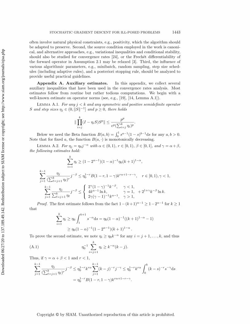
Copyright © by SIAM. Unauthorized reproduction of this article is prohibited.
STOCHASTIC GRADIENT DESCENT FOR ILL-POSED PROBLEMS 1443
often involve natural physical constraints, e.g., positivity, which the algorithm shouldbe adapted to preserve. Second, the source condition employed in the work is canoni-cal, and alternative approaches, e.g., variational inequalities and conditional stability,should also be studied for convergence rates [24], or the Frech\'et differentiability ofthe forward operator in Assumption 2.1 may be relaxed [3]. Third, the influence ofvarious algorithmic parameters, e.g., minibatch, random sampling, step size sched-ules (including adaptive rules), and a posteriori stopping rule, should be analyzed toprovide useful practical guidelines.
Appendix A. Auxiliary estimates. In this appendix, we collect severalauxiliary inequalities that have been used in the convergence rates analysis. Mostestimates follow from routine but rather tedious computations. We begin with awell-known estimate on operator norms (see, e.g., [19], [14, Lemma A.1]).
Lemma A.1. For any j < k and any symmetric and positive semidefinite operatorS and step sizes \eta j \in (0, \| S\| - 1] and p \geq 0, there holds
\| k\prod
i=j
(I - \eta iS)Sp\| \leq pp
ep(\sum k
i=j \eta i)p.
Below we need the Beta function B(a, b) =\int 1
0sa - 1(1 - s)b - 1ds for any a, b > 0.
Note that for fixed a, the function B(a, \cdot ) is monotonically decreasing.
Lemma A.2. For \eta j = \eta 0j - \alpha with \alpha \in (0, 1), r \in [0, 1), \beta \in [0, 1], and \gamma = \alpha +\beta ,
the following estimates hold:
k\sum i=1
\eta i \geq (1 - 2\alpha - 1)(1 - \alpha ) - 1\eta 0(k + 1)1 - \alpha ,
k - 1\sum j=1
\eta j
(\sum k
\ell =j+1 \eta \ell )rj - \beta \leq \eta 1 - r
0 B(1 - r, 1 - \gamma )kr\alpha +1 - r - \gamma , r \in [0, 1), \gamma < 1,
k - 1\sum j=1
\eta j\sum k\ell =j+1 \eta \ell
j - \beta \leq
\left\{ 2\gamma (1 - \gamma ) - 1k - \beta , \gamma < 1,4k\alpha - 1 ln k, \gamma = 1,2\gamma (\gamma - 1) - 1k\alpha - 1, \gamma > 1,
+ 21+\gamma k - \beta ln k.
Proof. The first estimate follows from the fact 1 - (k+1)\alpha - 1 \geq 1 - 2\alpha - 1 for k \geq 1that
k\sum i=1
\eta i \geq \eta 0
\int k+1
1
s - \alpha ds = \eta 0(1 - \alpha ) - 1((k + 1)1 - \alpha - 1)
\geq \eta 0(1 - \alpha ) - 1(1 - 2\alpha - 1)(k + 1)1 - \alpha .
To prove the second estimate, we note \eta i \geq \eta 0k - \alpha for any i = j + 1, . . . , k, and thus
(A.1) \eta - 10
k\sum i=j+1
\eta i \geq k - \alpha (k - j).
Thus, if \gamma = \alpha + \beta < 1 and r < 1,
k - 1\sum j=1
\eta j
(\sum k
\ell =j+1 \eta \ell )rj - \beta \leq \eta 1 - r
0 kr\alpha k - 1\sum j=1
(k - j) - rj - \gamma \leq \eta 1 - r0 kr\alpha
\int k
0
(k - s) - rs - \gamma ds
= \eta 1 - r0 B(1 - r, 1 - \gamma )kr\alpha +1 - r - \gamma .
Dow
nloa
ded
06/2
7/20
to 1
37.1
89.4
9.14
2. R
edis
trib
utio
n su
bjec
t to
SIA
M li
cens
e or
cop
yrig
ht; s
ee h
ttp://
ww
w.s
iam
.org
/jour
nals
/ojs
a.ph
p

Copyright © by SIAM. Unauthorized reproduction of this article is prohibited.
1444 BANGTI JIN, ZEHUI ZHOU, AND JUN ZOU
Similarly, if r = 1, it follows from (A.1) that
k - 1\sum j=1
\eta j\sum k\ell =j+1 \eta \ell
j - \beta \leq k\alpha k - 1\sum j=1
(k - j) - 1j - \gamma
= k\alpha [ k2 ]\sum j=1
j - \gamma (k - j) - 1 + k\alpha k - 1\sum
j=[ k2 ]+1
j - \gamma (k - j) - 1
\leq 2k\alpha - 1
[ k2 ]\sum j=1
j - \gamma + 2\gamma k - \beta k - 1\sum
j=[ k2 ]+1
(k - j) - 1.
Simple computation gives
(A.2)
k - 1\sum j=[ k2 ]+1
(k - j) - 1 \leq 2 ln k and
[ k2 ]\sum j=1
j - \gamma \leq
\left\{ (1 - \gamma ) - 1(k2 )1 - \gamma , \gamma \in [0, 1),
2 ln k, \gamma = 1,\gamma (\gamma - 1) - 1, \gamma > 1.
Combining the last three estimates gives the assertion for the case r = 1.
Next we recall two useful estimates.
Lemma A.3. For \eta j = \eta 0j - \alpha with \alpha \in (0, 1), \beta \in [0, 1], and r \geq 0, there hold
[ k2 ]\sum j=1
\eta 2j
(\sum k
\ell =j+1 \eta \ell )rj - \beta \leq c\alpha ,\beta ,rk
- r(1 - \alpha )+max(0,1 - 2\alpha - \beta ),
k - 1\sum j=[ k2 ]+1
\eta 2j
(\sum k
\ell =j+1 \eta \ell )rj - \beta \leq c\prime \alpha ,\beta ,rk
- ((2 - r)\alpha +\beta )+max(0,1 - r),
where we slightly abuse the notation k - max(0,0) for ln k and c\alpha ,\beta ,r and c\prime \alpha ,\beta ,r are givenby
c\alpha ,\beta ,r = 2r\eta 2 - r0
\left\{ 2\alpha +\beta
2\alpha +\beta - 1 , 2\alpha + \beta > 1,
2, 2\alpha + \beta = 1,22\alpha +\beta - 1
1 - 2\alpha - \beta , 2\alpha + \beta < 1,
and c\prime \alpha ,\beta ,r = 22\alpha +\beta \eta 2 - r0
\left\{ r
r - 1 , r > 1,
2, r = 1,2r - 1
1 - r , r < 1.
Proof. The proof is based on (A.1) and (A.2) and essentially given in [14, LemmaA.3], but the constants are corrected.
The next result collects some lengthy estimates needed in the proof of Theo-rem 4.8.
Proposition A.1. Let \beta = min(2\nu (1 - \alpha ), \alpha - \epsilon ), \gamma = min((1+2\nu )(1 - \alpha ), 1 - \epsilon ),and r = min( 12+\nu , 1 - \epsilon
2(1 - \alpha ) ). Then under the conditions in Theorem 4.8, i.e., \| B\| \leq 1,
\eta 0 \leq 1, and \theta being sufficiently small, with \zeta = ( 12 - \nu )(1 - \alpha ), the following estimates
Dow
nloa
ded
06/2
7/20
to 1
37.1
89.4
9.14
2. R
edis
trib
utio
n su
bjec
t to
SIA
M li
cens
e or
cop
yrig
ht; s
ee h
ttp://
ww
w.s
iam
.org
/jour
nals
/ojs
a.ph
p

Copyright © by SIAM. Unauthorized reproduction of this article is prohibited.
STOCHASTIC GRADIENT DESCENT FOR ILL-POSED PROBLEMS 1445
hold:
k\sum j=1
\eta j\phi 12j j
- \gamma 2 \leq c1(k + 1) -
\beta 2 ,
k\sum j=1
\eta 2j (\phi 12j )
2j - \gamma \leq c2(k + 1) - \beta ,
(A.3)
[ k2 ]\sum j=1
\eta 2j (\phi rj)
2j - \gamma +
k\sum j=[ k2 ]+1
\eta 2j (\phi 12j )
2j - \gamma \leq c3(k + 1) - \gamma ,
k\sum j=1
\eta j\phi 1jj
- \beta +\gamma 2 \leq c4(k + 1) -
\gamma 2 ,
(A.4)
\biggl( k\sum i=1
\eta i\phi 1i i
- \gamma 2
\biggr) \biggl( k\sum j=1
\eta j\phi 1jj
- \gamma +\theta \beta 2
\biggr) \leq c5(k + 1) - \gamma ,
k\sum j=1
\eta j\phi 1jj
- \gamma +\theta \beta 2 \leq c6(k + 1) -
\gamma 2 ,
(A.5)
with c1 = 2\beta 2 \eta
120 (2
- 1B( 12 , \zeta ) + 1), c2 = 2\beta \eta 0(\alpha - 1 + 2), c3 = 2\gamma \eta 2 - 2r
0 (3\alpha - 1 + 1),
c4 = 2\gamma 2
\bigl( \zeta - 1 + 2\beta - 1 + 1), c5 = 2\gamma ((( 12 - \nu - \theta \nu )(1 - \alpha )) - 1 + 4(\theta \beta ) - 1 + 1)2, and
c6 = 2\gamma 2 (\zeta - 1 + 2(\theta \beta ) - 1 + 1).
Proof. It follows from Lemma A.1 and the condition \| B\| \leq 1 that
k\sum j=1
\eta j\phi 12j j
- \gamma 2 \leq (2e) -
12
k - 1\sum j=1
\eta j
(\sum k
\ell =1 \eta \ell )12
j - \gamma 2 + \eta 0k
- \alpha - \gamma 2
\leq (\eta 120 2
- 1B( 12 , 1 - \alpha - \gamma 2 ) + \eta 0)k
1 - \alpha 2 - \gamma
2 .
By the definitions of \beta and \gamma , we have 1 - \alpha 2 - \gamma
2 = - \beta 2 and 1 - \alpha - \gamma
2 \geq ( 12 - \nu )(1 - \alpha ) := \zeta .Thus, the monotonicity of the Beta function and the inequality 2k \geq k + 1 for k \geq 1imply the first inequality of (A.3). Now by Lemmas A.1 and A.3,
k\sum j=1
\eta 2j (\phi 12j )
2j - \gamma \leq (2e) - 1k - 1\sum j=1
\eta 2j\sum k\ell =j+1 \eta j
j - \gamma + \eta 20\| B12 \| 2k - 2\alpha - \gamma
(A.6)
\leq \eta 0
\Bigl( (2e) - 1 2(2\alpha + \gamma )
2\alpha + \gamma - 1k - (1 - \alpha ) + (2e) - 121+2\alpha +\gamma k - \alpha - \gamma ln k + \eta 0\| B
12 \| 2k - 2\alpha - \gamma
\Bigr) .
Now, for any r > 0, there holds
(A.7) s - r ln s \leq (er) - 1 \forall s \geq 0,
and thus k - \alpha - \gamma ln k = k - \beta (k - 1 ln k) \leq e - 1k - \beta . Further, by the definition of \gamma ,2\alpha + \gamma \leq min(2, 1 + 2\alpha ) \leq 2, and since \epsilon < \alpha
2 , 2\alpha + \gamma - 1 \geq \alpha ,
(A.8) 2\alpha +\gamma 2\alpha +\gamma - 1 = 1 + 1
2\alpha +\gamma - 1 \leq 1 + \alpha - 1.
Then the last three estimates (with \| B\| \leq 1) imply
k\sum j=1
\eta 2j (\phi 12j )
2j - \gamma \leq 2\beta \eta 0\bigl( \alpha - 1 + 2
\bigr) (k + 1) - \beta .
This proves the second inequality in (A.3).
Dow
nloa
ded
06/2
7/20
to 1
37.1
89.4
9.14
2. R
edis
trib
utio
n su
bjec
t to
SIA
M li
cens
e or
cop
yrig
ht; s
ee h
ttp://
ww
w.s
iam
.org
/jour
nals
/ojs
a.ph
p
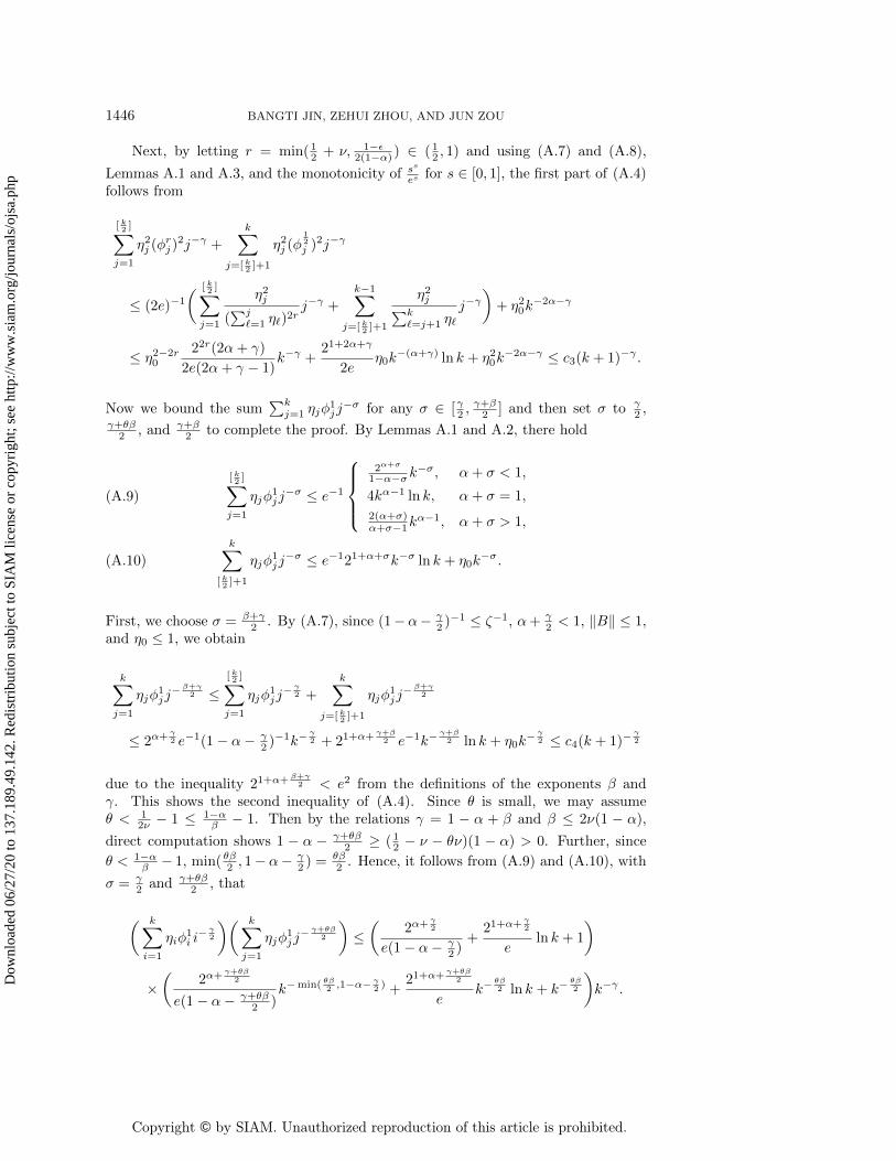
Copyright © by SIAM. Unauthorized reproduction of this article is prohibited.
1446 BANGTI JIN, ZEHUI ZHOU, AND JUN ZOU
Next, by letting r = min( 12 + \nu , 1 - \epsilon 2(1 - \alpha ) ) \in ( 12 , 1) and using (A.7) and (A.8),
Lemmas A.1 and A.3, and the monotonicity of ss
es for s \in [0, 1], the first part of (A.4)follows from
[ k2 ]\sum j=1
\eta 2j (\phi rj)
2j - \gamma +
k\sum j=[ k2 ]+1
\eta 2j (\phi 12j )
2j - \gamma
\leq (2e) - 1
\biggl( [ k2 ]\sum j=1
\eta 2j
(\sum j
\ell =1 \eta \ell )2rj - \gamma +
k - 1\sum j=[ k2 ]+1
\eta 2j\sum k\ell =j+1 \eta \ell
j - \gamma
\biggr) + \eta 20k
- 2\alpha - \gamma
\leq \eta 2 - 2r0
22r(2\alpha + \gamma )
2e(2\alpha + \gamma - 1)k - \gamma +
21+2\alpha +\gamma
2e\eta 0k
- (\alpha +\gamma ) ln k + \eta 20k - 2\alpha - \gamma \leq c3(k + 1) - \gamma .
Now we bound the sum\sum k
j=1 \eta j\phi 1jj
- \sigma for any \sigma \in [\gamma 2 ,\gamma +\beta 2 ] and then set \sigma to \gamma
2 ,\gamma +\theta \beta
2 , and \gamma +\beta 2 to complete the proof. By Lemmas A.1 and A.2, there hold
[ k2 ]\sum j=1
\eta j\phi 1jj
- \sigma \leq e - 1
\left\{ 2\alpha +\sigma
1 - \alpha - \sigma k - \sigma , \alpha + \sigma < 1,
4k\alpha - 1 ln k, \alpha + \sigma = 1,
2(\alpha +\sigma )\alpha +\sigma - 1k
\alpha - 1, \alpha + \sigma > 1,
(A.9)
k\sum [ k2 ]+1
\eta j\phi 1jj
- \sigma \leq e - 121+\alpha +\sigma k - \sigma ln k + \eta 0k - \sigma .(A.10)
First, we choose \sigma = \beta +\gamma 2 . By (A.7), since (1 - \alpha - \gamma
2 ) - 1 \leq \zeta - 1, \alpha + \gamma
2 < 1, \| B\| \leq 1,and \eta 0 \leq 1, we obtain
k\sum j=1
\eta j\phi 1jj
- \beta +\gamma 2 \leq
[ k2 ]\sum j=1
\eta j\phi 1jj
- \gamma 2 +
k\sum j=[ k2 ]+1
\eta j\phi 1jj
- \beta +\gamma 2
\leq 2\alpha +\gamma 2 e - 1(1 - \alpha - \gamma
2 ) - 1k -
\gamma 2 + 21+\alpha + \gamma +\beta
2 e - 1k - \gamma +\beta
2 ln k + \eta 0k - \gamma
2 \leq c4(k + 1) - \gamma 2
due to the inequality 21+\alpha + \beta +\gamma 2 < e2 from the definitions of the exponents \beta and
\gamma . This shows the second inequality of (A.4). Since \theta is small, we may assume\theta < 1
2\nu - 1 \leq 1 - \alpha \beta - 1. Then by the relations \gamma = 1 - \alpha + \beta and \beta \leq 2\nu (1 - \alpha ),
direct computation shows 1 - \alpha - \gamma +\theta \beta 2 \geq ( 12 - \nu - \theta \nu )(1 - \alpha ) > 0. Further, since
\theta < 1 - \alpha \beta - 1, min( \theta \beta 2 , 1 - \alpha - \gamma
2 ) =\theta \beta 2 . Hence, it follows from (A.9) and (A.10), with
\sigma = \gamma 2 and \gamma +\theta \beta
2 , that
\biggl( k\sum i=1
\eta i\phi 1i i
- \gamma 2
\biggr) \biggl( k\sum j=1
\eta j\phi 1jj
- \gamma +\theta \beta 2
\biggr) \leq
\biggl( 2\alpha +
\gamma 2
e(1 - \alpha - \gamma 2 )
+21+\alpha + \gamma
2
eln k + 1
\biggr)
\times \biggl(
2\alpha +\gamma +\theta \beta
2
e(1 - \alpha - \gamma +\theta \beta 2 )
k - min( \theta \beta 2 ,1 - \alpha - \gamma
2 ) +21+\alpha + \gamma +\theta \beta
2
ek -
\theta \beta 2 ln k + k -
\theta \beta 2
\biggr) k - \gamma .
Dow
nloa
ded
06/2
7/20
to 1
37.1
89.4
9.14
2. R
edis
trib
utio
n su
bjec
t to
SIA
M li
cens
e or
cop
yrig
ht; s
ee h
ttp://
ww
w.s
iam
.org
/jour
nals
/ojs
a.ph
p

Copyright © by SIAM. Unauthorized reproduction of this article is prohibited.
STOCHASTIC GRADIENT DESCENT FOR ILL-POSED PROBLEMS 1447
Then we move one factor k - \theta \beta 4 from the second bracket to the first and bound by
(A.7),\biggl( k\sum i=1
\eta i\phi 1i i
- \gamma 2
\biggr) \biggl( k\sum j=1
\eta j\phi 1jj
- \gamma +\theta \beta 2
\biggr) \leq
\biggl( 2\alpha +
\gamma 2
e(1 - \alpha - \gamma 2 )
+21+\alpha + \gamma
2
ek -
\theta \beta 4 ln k + 1
\biggr)
\times \biggl(
2\alpha +\gamma +\theta \beta
2
e(1 - \alpha - \gamma +\theta \beta 2 )
+21+\alpha + \gamma +\theta \beta
2
ek -
\theta \beta 4 ln k + 1
\biggr) k - \gamma
\leq 2\gamma ((( 12 - \nu - \theta \nu )(1 - \alpha )) - 1 + 4(\theta \beta ) - 1 + 1\bigr) 2(k + 1) - \gamma ,
proving the first inequality of (A.5). The other estimate in (A.5) follows similarly bychoosing \sigma = \gamma +\theta \beta
2 and hence is omitted.
Remark A.1. The proof of Proposition A.1 implies\sum k - 1
j=1 \eta j\phi 1jj
- \gamma 2 \leq (\zeta - 1 +
2 ln k)k - \gamma 2 . The log factor ln k seems not removable and precludes a direct application
of mathematical induction in the proof of Theorem 4.8. The extra factor j - \theta \beta 2 due
to Assumption 2.4 gracefully compensates the log factor ln k using (A.7). The small-ness condition on \theta can be removed at the expense of less transparent dependence.Specifically, by Lemma A.2, with \sigma = \alpha + \gamma +\theta \beta
2 , there holds
k\sum j=1
\eta j\phi 1jj
- \gamma +\theta \beta 2
\leq 1
ek\gamma 2
\left\{ 2\sigma
1 - \sigma k - \theta \beta
2 , \sigma < 1
4k - (1 - \alpha - \gamma 2 ) ln k, \sigma = 1
2\sigma \sigma - 1k
- (1 - \alpha - \gamma 2 ), \sigma > 1
+ 21+\sigma e - 1k - \gamma 2 -
\theta \beta 2 ln k + k - (\alpha + \gamma +\theta \beta
2 ).
Instead of applying (A.7) directly, we rearrange the terms and discuss the cases \sigma < 1,\sigma = 1, and \sigma > 1 separately with the argument in the proof of Proposition A.1 andobtain \biggl( k\sum
i=1
\eta i\phi 1i i
- \gamma 2
\biggr) \biggl( k\sum j=1
\eta j\phi 1jj
- \gamma +\theta \beta 2
\biggr) \leq c\sigma 2
\gamma (k + 1) - \gamma ,
with the constant c\sigma given by
c\sigma =
\left\{ (1 - \sigma ) - 1 + 4(\theta \beta ) - 1 + 1, \sigma < 1,\zeta - 1 + 8(\theta \beta ) - 1 + 1, \sigma = 1,2(\sigma - 1) - 1 + 3\zeta - 1 + 1, \sigma > 1.
The next result gives some basic estimates used in the proof of Theorem 2.5.
Proposition A.2. Under the induction hypothesis of Theorem 2.5 and (4.20),there hold
ak+1 \leq \Bigl( (c1(c0\varrho + (cR\varrho
12 + 1)\| w\| ) + c\nu \| w\| )2 + 2n(c2\varrho + c3\| w\| 2)
+ 2nc21\bigl( \varrho
12 + \| w\|
\bigr) \bigl( c0\varrho
12 + cR\| w\|
\bigr) \varrho
\theta 2 + nc21(c0\varrho
12 + cR\| w\| )2\varrho \theta
\Bigr) (k + 1) - \beta ,
bk+1 \leq \Bigl( (c0c
\prime 1\varrho + c\prime 5(cR\varrho
12 + 1)\| w\| + c\nu \| w\| )2 + 2n(c\prime 2\varrho + c3\| w\| 2) + 2n(c\prime 3\varrho
12 + c\prime 5\| w\| )
\times (c0c\prime 3\varrho
12 + c\prime 5cR\| w\| )\varrho
\theta 2 + n(c0c
\prime 4\varrho
12 + c\prime 5cR\| w\| )2\varrho \theta
\Bigr) (k + 1) - \gamma ,
where the constants c1, c2, c3, and c\prime 1, . . . , c\prime 5 are given in the proof.
Dow
nloa
ded
06/2
7/20
to 1
37.1
89.4
9.14
2. R
edis
trib
utio
n su
bjec
t to
SIA
M li
cens
e or
cop
yrig
ht; s
ee h
ttp://
ww
w.s
iam
.org
/jour
nals
/ojs
a.ph
p

Copyright © by SIAM. Unauthorized reproduction of this article is prohibited.
1448 BANGTI JIN, ZEHUI ZHOU, AND JUN ZOU
Proof. First, it follows directly from Lemmas A.1, A.2, and A.3 and the assump-tions \| B\| \leq 1 and \eta 0 \leq 1 that for any \sigma \in [0, 1 - \alpha ),
k\sum j=1
\eta j\phi 12j j
- \sigma \leq \eta 120 (2
- 1B( 12 , 1 - \alpha - \sigma ) + 1)k1 - \alpha 2 - \sigma ,(A.11)
k\sum j=1
\eta 2j (\phi 12j )
2 \leq \eta 0(| 1 - 2\alpha | - 1 + \alpha - 1 + 1) := c3,(A.12)
where we have abused the writing 0 - 1 for 1. Meanwhile, by Proposition A.1, we have
k\sum j=1
\eta j\phi 12j j
- \gamma 2 \leq c1(k + 1) -
\beta 2 and
k\sum j=1
\eta 2j (\phi 12j )
2j - \gamma \leq c2(k + 1) - \beta ,(A.13)
with c1 = 2\beta 2 \eta
120 (2
- 1B( 12 , \zeta ) + 1), \zeta = ( 12 - \nu )(1 - \alpha ), and c2 = 2\beta \eta 0(\alpha - 1 + 2). By
(A.11)--(A.13) and the monotonicity of the Beta function and k + 1 \leq k\ast (cf. (4.20)),we obtain
k\sum j=1
\eta j\phi 12j
\bigl( c0\varrho j
- \beta +\gamma 2 + cR\varrho
12 j -
\beta 2 \delta + \delta
\bigr) \leq c0c1\varrho (k + 1) -
\beta 2 + (cR\varrho
12 + 1)c1(k + 1)
1 - \alpha 2 \delta
\leq c1\bigl( c0\varrho + (cR\varrho
12 + 1)\| w\|
\bigr) (k + 1) -
\beta 2 ,
k\sum j=1
\eta 2j (\phi 12j )
2(\varrho 12 j -
\gamma 2 + \delta )2 \leq 2(c2\varrho + c3\| w\| 2)(k + 1) - \beta .
Likewise, by the monotonicity of the Beta function, we deduce\biggl( k\sum i=1
\eta i\phi 12i (\varrho
12 i -
\gamma 2 + \delta )
\biggr) \biggl( k\sum j=1
\eta j\phi 12j (c0\varrho
12 j -
\gamma 2 + cR\delta )\varrho
\theta 2 j -
\theta \beta 2
\biggr) \leq c21(\varrho
12 + \| w\| )(c0\varrho
12 + cR\| w\| )\varrho
\theta 2 (k + 1) - \beta ,
k\sum j=1
\eta j\phi 12j (c0\varrho
12 j -
\gamma 2 + cR\delta )\varrho
\theta 2 j -
\theta \beta 2 \leq c1(c0\varrho
12 + cR\| w\| )\varrho
\theta 2 (k + 1) -
\beta 2 .
The last four estimates give (4.21). Now we prove (4.23). By Proposition A.1, wehave
k\sum j=1
\eta j\phi 1jj
- \beta +\gamma 2 \leq c\prime 1(k + 1) -
\gamma 2 ,
[ k2 ]\sum j=1
\eta 2j (\phi rj)
2j - \gamma +
k\sum j=[ k2 ]+1
\eta 2j (\phi 12j )
2j - \gamma \leq c\prime 2(k + 1) - \gamma ,
\biggl( k\sum i=1
\eta i\phi 1i i
- \gamma 2
\biggr) \biggl( k\sum j=1
\eta j\phi 1jj
- \gamma +\theta \beta 2
\biggr) \leq c\prime 23 (k + 1) - \gamma ,
k\sum j=1
\eta j\phi 1jj
- \gamma +\theta \beta 2 \leq c\prime 4(k + 1) -
\gamma 2 ,
with c\prime 1 = 2\gamma 2 (\zeta - 1 + 2\beta - 1 + 1), c\prime 2 = 2\gamma \eta 2 - 2r
0 (3\alpha - 1 + 1), c\prime 3 = 2\gamma 2 ((( 12 - \nu - \theta \nu )(1 -
\alpha )) - 1+4(\theta \beta ) - 1+1), and c\prime 4 = 2\gamma 2 (\zeta - 1+2(\theta \beta ) - 1+1). Further, by (A.9) and (A.10),
for any \sigma \in [0, \gamma 2 ],
k - \nu (1 - \alpha )k\sum
j=1
\eta j\phi 1jj
- \sigma \leq \zeta - 1 + 2(\nu (1 - \alpha )) - 1 + 1 := c\prime 5.
Dow
nloa
ded
06/2
7/20
to 1
37.1
89.4
9.14
2. R
edis
trib
utio
n su
bjec
t to
SIA
M li
cens
e or
cop
yrig
ht; s
ee h
ttp://
ww
w.s
iam
.org
/jour
nals
/ojs
a.ph
p

Copyright © by SIAM. Unauthorized reproduction of this article is prohibited.
STOCHASTIC GRADIENT DESCENT FOR ILL-POSED PROBLEMS 1449
With these estimates and (4.20), we deduce
k\sum j=1
\eta j\phi 1j
\bigl( c0\varrho j
- \beta +\gamma 2 + cR\varrho
12 j -
\beta 2 \delta + \delta
\bigr) \leq (c0c
\prime 1\varrho + c\prime 5(cR\varrho
12 + 1)\| w\| )(k + 1) -
\gamma 2 ,
k\sum j=1
\eta 2j (\phi 1j )
2(\varrho 12 j -
\gamma 2 + \delta )2 \leq 2(c\prime 2\varrho + c3\| w\| 2)(k + 1) - \gamma ,
k\sum j=1
\eta j\phi 1j (c0\varrho
12 j -
\gamma 2 + cR\delta )\varrho
\theta 2 j -
\theta \beta 2 \leq (c0c
\prime 4\varrho
12 + c\prime 5cR\| w\| )\varrho
\theta 2 (k + 1) -
\gamma 2 ,
where the second line is due to (A.12) and the inequality\sum k
j=1 \eta 2j (\phi
1j )
2 \leq \sum k
j=1 \eta 2j (\phi
12j )
2
(since \| B\| \leq 1). Finally, repeating the argument in Proposition A.1 gives\biggl( k\sum i=1
\eta i\phi 1i (\varrho
12 i -
\gamma 2 + \delta )
\biggr) \biggl( k\sum j=1
\eta j\phi 1j (c0\varrho
12 j -
\gamma 2 + cR\delta )\varrho
\theta 2 j -
\theta \beta 2
\biggr) \leq (c\prime 3\varrho
12 + c\prime 5\| w\| )(c0c\prime 3\varrho
12 + c\prime 5cR\| w\| )\varrho
\theta 2 (k + 1) - \gamma .
Then combining the last four estimates yields the desired bound on bk+1.
Acknowledgments. The authors are grateful to the associate editor, ProfessorFrank E. Curtis, and two anonymous referees for helpful comments.
REFERENCES
[1] L. Bottou, F. E. Curtis, and J. Nocedal, Optimization methods for large-scale machinelearning, SIAM Rev., 60 (2018), pp. 223--311, https://doi.org/10.1137/16M1080173.
[2] K. Chen, Q. Li, and J.-G. Liu, Online learning in optical tomography: A stochastic approach,Inverse Problems, 34 (2018), 075010.
[3] C. Clason and V. H. Nhu, Bouligand--Landweber iteration for a non-smooth ill-posed problem,Numer. Math., 142 (2019), pp. 789--832.
[4] A. Dieuleveut and F. Bach, Nonparametric stochastic approximation with large step-sizes,Ann. Statist., 44 (2016), pp. 1363--1399, https://doi.org/10.1214/15-AOS1391.
[5] H. W. Engl, M. Hanke, and A. Neubauer, Regularization of Inverse Problems, Kluwer,Dordrecht, The Netherlands, 1996.
[6] C. Geiersbach and G. C. Pflug, Projected stochastic gradients for convex constrained prob-lems in Hilbert spaces, SIAM J. Optim., 29 (2019), pp. 2079--2099, https://doi.org/10.1137/18M1200208.
[7] R. M. Gower, N. Loizou, X. Qian, A. Sailanbayev, E. Shulgin, and P. Richt\'arik, SGD:General analysis and improved rates, in Proceedings of the 36th International Conferenceon Machine Learning, PMLR 97, K. Chaudhuri and R. Salakhutdinov, eds., Long Beach,CA, 2019, pp. 5200--5209.
[8] M. Hanke, A. Neubauer, and O. Scherzer, A convergence analysis of the Landweber it-eration for nonlinear ill-posed problems, Numer. Math., 72 (1995), pp. 21--37, https://doi.org/10.1007/s002110050158.
[9] G. T. Herman, A. Lent, and P. H. Lutz, Relaxation method for image reconstruction, Comm.ACM, 21 (1978), pp. 152--158, https://doi.org/10.1145/359340.359351.
[10] G. T. Herman and L. B. Meyer, Algebraic reconstruction techniques can be made computa-tionally efficient, IEEE Trans. Med. Imaging, 12 (1993), pp. 600--609.
[11] K. Ito and B. Jin, A new approach to nonlinear constrained Tikhonov regularization, InverseProblems, 27 (2011), 105005, https://doi.org/10.1088/0266-5611/27/10/105005.
[12] K. Ito and B. Jin, Inverse Problems: Tikhonov Theory and Algorithms, World Scientific,Hackensack, NJ, 2015.
[13] Y. Jiao, B. Jin, and X. Lu, Preasymptotic convergence of randomized Kaczmarz method,Inverse Problems, 33 (2017), 125012.
Dow
nloa
ded
06/2
7/20
to 1
37.1
89.4
9.14
2. R
edis
trib
utio
n su
bjec
t to
SIA
M li
cens
e or
cop
yrig
ht; s
ee h
ttp://
ww
w.s
iam
.org
/jour
nals
/ojs
a.ph
p

Copyright © by SIAM. Unauthorized reproduction of this article is prohibited.
1450 BANGTI JIN, ZEHUI ZHOU, AND JUN ZOU
[14] B. Jin and X. Lu, On the regularizing property of stochastic gradient descent, Inverse Problems,35 (2019), 015004.
[15] B. Kaltenbacher, A. Neubauer, and O. Scherzer, Iterative Regularization Methods forNonlinear Ill-Posed Problems, Walter de Gruyter, Berlin, 2008, https://doi.org/10.1515/9783110208276.
[16] D. P. Kingma and J. Ba, Adam: A method for stochastic optimization, in Proceedings of the3rd International Conference on Learning Representations (ICLR), San Diego, CA, 2015.
[17] H. J. Kushner and G. G. Yin, Stochastic Approximation and Recursive Algorithms andApplications, 2nd ed., Springer-Verlag, New York, 2003.
[18] L. Landweber, An iteration formula for Fredholm integral equations of the first kind, Amer.J. Math., 73 (1951), pp. 615--624, https://doi.org/10.2307/2372313.
[19] J. Lin and L. Rosasco, Optimal rates for multi-pass stochastic gradient methods, J. Mach.Learn. Res., 18 (2017), pp. 1--47.
[20] A. K. Louis, Inverse und Schlecht Gestellte Probleme, B. G. Teubner, Stuttgart, 1989, https://doi.org/10.1007/978-3-322-84808-6.
[21] S. F. McCormick and G. H. Rodrigue, A uniform approach to gradient methods for linearoperator equations, J. Math. Anal. Appl., 49 (1975), pp. 275--285, https://doi.org/10.1016/0022-247X(75)90179-1.
[22] H. Robbins and S. Monro, A stochastic approximation method, Ann. Math. Stat., 22 (1951),pp. 400--407.
[23] O. Scherzer, M. Grasmair, H. Grossauer, M. Haltmeier, and F. Lenzen, VariationalMethods in Imaging, Springer, New York, 2009.
[24] T. Schuster, B. Kaltenbacher, B. Hofmann, and K. S. Kazimierski, RegularizationMethods in Banach Spaces, Walter de Gruyter, Berlin, 2012, https://doi.org/10.1515/9783110255720.
[25] T. Strohmer and R. Vershynin, A randomized Kaczmarz algorithm with exponentialconvergence, J. Fourier Anal. Appl., 15 (2009), pp. 262--278, https://doi.org/10.1007/s00041-008-9030-4.
[26] I. Sutskever, J. Martens, G. Dahl, and G. E. Hinton, On the importance of initializationand momentum in deep learning, in Proceedings of the 30th International Conference onMachine Learning (ICML-13), S. Dasgupta and D. Mcallester, eds., Atlanta, GA, 2013,pp. 1139--1147.
[27] Y. S. Tan and R. Vershynin, Phase retrieval via randomized Kaczmarz: Theoretical guaran-tees, Inf. Inference, 8 (2019), pp. 97--123, https://doi.org/10.1093/imaiai/iay005.
[28] P. Tarr\`es and Y. Yao, Online learning as stochastic approximation of regularization paths:Optimality and almost-sure convergence, IEEE Trans. Inform. Theory, 60 (2014), pp. 5716--5735, https://doi.org/10.1109/TIT.2014.2332531.
[29] V. V. Vasin, Iterative methods for solving ill-posed problems with a priori information inHilbert spaces, Zh. Vychisl. Mat. Mat. Fiz., 28 (1988), pp. 971--980, 1117, https://doi.org/10.1016/0041-5553(88)90104-8.
[30] G. M. Va\u {\i}nikko and A. Y. Veretennikov, Iteration Procedures in Ill-Posed Problems,``Nauka,"" Moscow, 1986.
[31] Y. Ying and M. Pontil, Online gradient descent learning algorithms, Found. Comput. Math.,8 (2008), pp. 561--596, https://doi.org/10.1007/s10208-006-0237-y.
[32] T. Zhang, Solving large scale linear prediction problems using stochastic gradient descent algo-rithms, in Proceedings of the Twenty First International Conference on Machine Learning,C. Brodley, ed., Banff, AB, Canada, 2004, pp. 919--926.
Dow
nloa
ded
06/2
7/20
to 1
37.1
89.4
9.14
2. R
edis
trib
utio
n su
bjec
t to
SIA
M li
cens
e or
cop
yrig
ht; s
ee h
ttp://
ww
w.s
iam
.org
/jour
nals
/ojs
a.ph
p