on the constraint algebra of quantum gravity in the loop...

N U C L E A R PHYSICS B

ELSEVIER Nuclear Physics B 474 (1996) 249-268

On the constraint algebra of quantum gravity in the loop representation

B e r n d B r t i g m a n n ~ Max-Planck-lnstitut.[~r Gravitationsphysik, Schlaatzweg I, 14473 Potsdam, Germany

Received 12 January t996; accepted I May 1996

Abstract

Although an important issue in canonical quantization, the problem of representing the constraint algebra in the loop representation of quantum gravity has received little attention. The only explicit computation was performed by Gambini, Garat, and Pullin for a formal point-splitting regularization of the diffeomorphism and Hamiltonian constraints. It is shown that the calculation of the algebra simplifies considerably when the constraints are expressed not in terms of generic area derivatives but rather as the specific shift operators that reflect the geometric meaning of the constraints.

PACS: 04.60.+n Keywords: Canonical quantum gravity; Quantum constraint algebra

1. Introduct ion

A key problem of canonical quantization is the incorporation of the classical con-

straints. In general, we have to expect that there are many different and in their outcome

genuinely inequivalent ways to import classical symmetries into a quantum theory (for

a recent example, see Ref. [ 1 ] ), and a famous example for the resolution of such am-

biguities is the critical dimension of string theory, How to define and how to regulate

the constraint operators is directly related to the representation of the constraint algebra

in the quantum theory. Typically, the constraint operators are not uniquely determined

by the classical constraints, and demanding well-definedness of the quantum constraint

algebra is an important restriction on the choice of representation.

t E-mail: bruegman @ aei-potsdam.mpg.de.

0550-3213/96/$15.00 @, 1996 Elsevier Science B.V. All rights reserved PII S0550-32 1 3 ( 96)0024 1 -6

250 B. Bragmann/Nuclear Physics B 474 (1996) 249-268

Here we study the constraint algebra of vacuum general relativity in 3+I dimensions

in the framework of Dirac quantization, in which the classical constraints C are elevated to quantum operators C" and imposed as operator relations on the wave functions, C'~p = 0. Given a definition of the constraint operators, the question is whether there are

anomalies in the constraint algebra, and if so, how to treat them. Currently there are no rigorous results about the constraint algebra of quantum gravity because of difficulties to define the constraint operators, e.g., issues of factor ordering and regularization arise.

In the canonical formulation of vacuum general relativity there are two types of constraints, the three-dimensional diffeomorphism constraint D and the Hamiltonian constraint H, which satisfy the following algebra:

{O(v),D(w)}=D(E,,w), {D(v),H(N)}=H(E,,N),

{ H ( M ) , H ( N ) } = D (gabwt,),

(1)

(2)

(3)

where rob = MObN-Nc~bM, g~,h is the inverse three-metric, v and w are vector fields, and

M and N are scalar densities of weight - 1 , all on a three-manifold which we choose to be compact.

The constraint algebra of general relativity has two important features. First, the

algebra closes but only for structure functions containing one of the geometric variables

in (3). And second, neither D nor H form an ideal, and therefore one cannot construct

a reduced phase space with respect to just one of the constraints. For example, the diffeomorphism constraint would form an ideal if the constraint on the right-hand side

of (2) was D, but as it stands, there are no invariant subspaces that are necessary for phase space reduction.

For canonical quantization of general relativity a very fruitful approach has turned

out to be the Rovelli-Smolin loop representation [2] based on the Ashtekar variables

[3,4]. For a motivation of the loop representation and a discussion of its strong and

weak points, see for example Ref. [5]. In this paper we locus on the technical problem of how to construct the quantum constraint operators in the loop representation, and

present a formal calculation of the constraint algebra in the loop representation. The loop representation, in which states are functionals of loops, can be obtained

from the connection representation, in which states are functionals of the Ashtekar connection, through the so-called loop transform. We introduce a for our purposes

particularly convenient form of the constraints via the transform. The level of our discussion remains on the same heuristic level as the original attempts to define the constraints [2,6-8]. In particular, the loop transform is not defined rigorously. Although

there now does exist a rigorous definition of the two representations and the loop transform based on distributional connections [9], which brings about certain changes

to the whole formalism, it is not yet known how to treat the Hamiltonian constraint rigorously. Note that the constraint operators in the loop representation can also be obtained without the loop transform directly from the Wilson-loop variables, with the

same result [ 10].

B. BrEigmann/Nuclear Physics B 474 (1996) 249-268 251

The definition of the constraint operators requires a regularization, and we use a point-splitting regularization. The problem with point splitting is that it introduces a background dependence which breaks diffeomorphism invariance and which survives in the limit that the regulators are removed. Further problems are that the constraint operators should act on a Hilbert space of states, but we do not have an inner product, and that the reality conditions of the Ashtekar formulation have not been implemented, and the constraint algebra of complex relativity might differ from that of real relativity. There have been important advances on these three issues (see, e.g., Refs. [11-13], respectively), but for the above reasons all calculations of the constraint algebra must still be called formal. What can be explored, however, is what the current framework predicts for the constraint algebra, and in the loop representation this is not a trivial task.

One can distinguish four approaches to the constraint algebra in the loop representation:

(i) Recall that in the connection representation the constraint algebra does close on a formal level without regularization [4]. One can hope that this feature is preserved by the loop transform (which is as we already pointed out still problematic for the Hamiltonian constraint). This justifies the route most commonly taken until quite recently, namely to postpone the treatment of the constraint algebra in the loop representation. Given the definition of the constraint operators in the loop

representation, one proceeds to study their kernel, to look for an inner product, defines observables, etc., without taking the constraint algebra into account.

(ii) Given the definition of the constraint operators in the loop representation, the constraint algebra is computed explicitly [6,14]. Blencowe [6] computes (2) only, using the group action of diffeomorphisms. Gambini, Garat, and Pullin [ 14] give a completely explicit computation of ( 1 ) - (3 ) . The technical difficulties encountered explain strategy (i). One problem is that the differential operator on the space of loop functionals that appears in the Hamiltonian constraint [6-8], the area derivative, is not very well studied, but now the machinery is available [15] that makes [14] possible.

(iii) One attempts a two-step procedure, first solving the diffeomorphism constraint, and then defining the Hamiltonian constraint operator only on the diffeomorphism- invariant states. This is how sometimes the original Rovelli-Smolin loop representation [2] is interpreted, namely as a theory of operators on knot invariants. For example, in the rigorous approach based on measures on the space of connections modulo gauge [ 12,16], the measures are constructed to be diffeomorphism invariant first, and one later attempts to construct a "diffeomorphism-invariant" Hamiltonian constraint operator. An analogous approach is taken in Loll's lattice gravity, which has led to important insights for certain geometric operators [ 17].

From the perspective of the quantum constraint algebra corresponding to ( 1 ) - (3), we have to observe that one cannot simply first impose the diffeomorphism constraint without consequences for the Hamiltonian constraint, since, as men- tioned above, the constraints are intertwined such that there are no ideals. Let

252 B. Briigmann/Nuclear Physics B 474 (1996) 249-268

us give a simple-minded example. Suppose that D(v)~ = 0 and that H(N)

does not map states out of the kernel of D(v), i.e. D(v)H(N) 0 = 0. Then

[ D (v ) ,H (N) ] = 0 , and by (2) , H(E~,N) =0 , which, since it holds for all v and

N, implies H(N) = 0. 2 That is, if we want to work exclusively on the space

of solutions to the diffeomorphism constraint, we have to consider the subspace

that is invariant under the Hamiltonian constraint, and then the constraint algebra implies that this subspace must be the simultaneous kernel of the constraints.

I f we want to define the symmetries of quantum gravity with the help of the

operator constraint algebra, we therefore have to implement the constraint algebra

before imposing the diffeomorphism constraint.

In this context it is perhaps worth pointing out that one of the main attractive

features of the loop representation, namely that a few non-trivial (formal) solutions

to both constraints are known, is not derived from a two-step implementation of

the constraints. Rather, one attempts to find the intersection of the kernels of the

constraints on the unreduced space of loop functionals [18].

(iv) One introduces (almost trivial) matter variables that allow the definition of a

preferred time slicing. The Hamiltonian constraint operator then turns into a proper

Hamiltonian operator, and the Wheeler-DeWitt equation into a proper Schr6dinger

equation [11]. The main advantage is that the regularized Hamiltonian operator

is diffeomorphism invariant, which opens up a whole range of interesting topics

in diffeornorphism-invariant dynamics. The problem of representing the constraint

algebra is easily solved because only the diffeomorphism algebra remains to be

represented, the information about the Hamiltonian constraint is now contained

in the Schr6dinger equation. In this sense, a preferred time slicing also defines

a two-step procedure. One should remember, and emphasize, however, that the

construction of matter clocks works only locally. The resulting theory is therefore

only an approximation to what is usually called full quantum gravity. It would

be very interesting to gain some control over the approximation, for example in

reduced models. Even so, the prospect of diffeomorphism-invariant dynamics is

very interesting, and may be physically quite relevant.

To summarize, one can either try to implement the classical constraints directly, (i)

and (ii), or to give a special treatment to the Hamiltonian constraint, (iii) and (iv). For

the latter, there are good motivations, like the observation that while the diffeomorphism

constraint is linear in the momenta and therefore generates a type of gauge symmetry,

the Hamiltonian constraint is quadratic in the momenta and does not possess simple

gauge orbits. Also, to obtain the conventional interpretation of time in quantum gravity

a special treatment of the Hamiltonian constraint may be necessary.

Here we do not choose to treat the constraints differently, but want to explore as in

(ii) whether the classical constraint algebra has a complete representation in the loop

representation of canonical quantum gravity. To state the outcome of the calculation, the

2 We thank A. Rendall for pointing out how a partition of unity allows one to extend the local integral of E,.N to the manifold such that any test function M may be written as E~N for some v and N.

B. Bri~'gmann/Nuclear Physics B 474 (1996) 249 268 253

resulting algebra maintains the structure of the classical algebra with a particular choice

of factor ordering for D(gabwb) , which becomes necessary because of the presence of

the metric. The level of rigor is equivalent to that in the connection representation, and upon removal of the point splitting there are no anomalies. Let us point out that the

formal nature of the point-splitting regularization does not allow us to decide whether

there actually are anomalies in the constraint algebra of quantum gravity.

Our contribution is to show that starting with a different form of the constraints the

result of Ref. [ 14] can be obtained in a simpler manner. The simplification comes about

by the observation that the constraints are not just based on generic area derivatives,

but rather on more specialized geometric operators, certain shift operators. This makes

the algebra manageable to the extent that the point-splitting regularization can now

be studied further along the lines of Ref. [19] , where the removal of the regulators

is examined in detail for the constraint algebra in the connection representation. In

terms of shift operators, the constraint operators may in fact be compatible with the

rigorous regularization techniques coming from distributional connections, with which

it is particularly hard to represent the field strength of the Ashtekar connection that

directly corresponds to the area derivative via the loop transform.

The paper is organized as follows. In Section 2 we define the constraints in the

connection and the loop representation and discuss the point-splitting regularization. In

Section 3 we introduce the basic loop derivative commutators. Section 4 contains the

calculation of the constraint algebra in the loop representation. In Section 5 we conclude

with a few comments.

2. The constraints and their representation

The constraints of quantum gravity in the loop representation have been derived in

various ways [2,6-8] with essentially the same result 3 . Since our method to compute

the constraint algebra depends crucially on the form of the constraint operators, let us

give a brief derivation via the loop transtorm.

The Ashtekar variables are a connection Ai~(x) and a vector density Eai(x) of weight

one, both complex, on a compact three-manifold 2;. Tangent space indices are denoted

by a, b . . . . . internal indices are denoted by i , j . . . . . The internal gauge group is SU(2) ,

and following Ref. [2] we choose generators r '~ such that

[ r i, r j ] = ei.JkT k. (4)

The algebra-valued variables are obtained by contraction, e.g., A, = Aia7 "i. The inverse

metric is given by

3 Based on Ref. [ 2 ], the constraints can be obtained through the loop transform or directly from the loop operators. In Ref. [ 7 ] the transform is used. In I 8 ] the constraints are derived from the loop operators and shown to be equivalent to Ref. [ 7 I. The very first derivation of the constraints in closed form in 161 can be understood as a hybrid of the two methods, giving the same result 1101.

254 B. Bragmann/Nuclear Physics B 474 (1996) 249-268

ggat, = EaiEbi ' (5)

where g is the determinant of g,,b (insuring the correct density weight). The constraints of general relativity which satisfy the algebra (1 ) - (3 ) are

= / d3x vaEhiFab + G(v), (6) D ( u)

H (N) = f d 3 x Ne ~ik EaiE I~i F~ b . ( 7 )

The vector constraint f d3x vaEbiF~d~ generates diffeomorphisms up to an internal gauge transformation, which is compensated by the term G(v), and a gauge-depending term also appears in (3). (The sign convention for the Poisson brackets in ( 1 ) - ( 3 ) is opposite to that of Ref. [4].)

In the connection representation, wave functions are functionals of the Ashtekar connection, ~/,[A], and the operators corresponding to the connection and the triad are represented by

~A~,(x) ' (8)

where h = 1 and a complex i has been absorbed in the definition of/~,i. The first non-trivial issue we have to face is regularization. While the type of point

splitting that we use has been commonly applied in many places, let us proceed slowly since there are different prescriptions for the order in which the various regulators have to be removed.

The necessity lor regularization arises at this point because the metric and the constraints are products of operators at the same point. We introduce a point splitting based on a background metric and a regulator f , ( x , y) satisfying

lira f~ (x, y) = 83 (x, y). (9) e~0

For the calculations that tbliow we fix a coordinate system and require that f~(x , y) is a smooth function of x - y.

As discussed in Refs. [20,21], which refer explicitly to the constraint algebra, a 'full' point splitting should be applied, that is, all points that appear in an operator product should be split. See also Ref. [22], where it is shown that only in a particular factor ordering is the connection representation related to the loop representation, and that the vector constraint in this factor ordering only gives rise to diffeomorphisms in the connection representation if a symmetric point splitting, f~(x , y) = f~ (y , x ) is employed. Following these considerations we define the operators

& ~ , ( x ) ; d3y d 3 z ' f ~ ( x ' Y ) f ~ ' ( x ' Z ) S a ~ , ( y ) S a ~ ( z ) ' (10)

D~(e) = - d3x d 3 y f ~ ( x , y ) v (x)~,~;77-7, F~l,(y) + G ( v ) , (11)

B. Brffgmann/Nuclear Physics B 474 (1996) 249 268 255

f f f H++,(N) = d3x d3y d3z fE(x ,y) f , , (x , z )N(x)e i#6aia(y ~ ~aj(z~

(12)

For the particular calculations that follow, some of the regulators can be removed since there do not arise singularities that require them. (As just recalled, this is not true for the vector constraint algebra in the connection representation.)

The transition to the loop representation is made via a formal transform, the loop transform

~/,[r/] = J DA tr U,70 [ A ] , (13)

where Un is the holonomy matrix of AI, around the loop r/,

u,7 = P exp f ds~"(s)A+,(~(s) ). (14)

In order to transfer the operators that we are interested in in the connection representation, Oc, to operators in the loop representation, OL, one performs a formal partial integration for any occurrence of a functional derivative with respect to A~, so that

OL0[r/]--- J D A t r U ~ O c ~ [ A ] = JT)A (O~trU~)O[A]. (15)

All that is needed for an explicit definition of OL as loop operator is a transfer relation of the operators on the Wilson loops that expresses the operation on the connection dependence of the Wilson loop purely as an operation on its loop dependence,

O+tr U~ = OLtr U~j. (16)

This construction is directly applicable to the metric and the constraints. The Wilson loop satisfies

+ ] ~Ai,(x----~trU~+ = ds~3(x, rl(s))'O~(s)tr(U~.~-ri), (17)

6 6rl~,( s-----~tr U~ =~)b ( s) F~,b( rl( s) )tr( U,.,ri), (18)

where Uss denotes the holonomy from rl(s) once around the loop. Variations of the Wilson loop with respect to the connection and the loop are not completely unrelated, and for the operators under considerations there exist transfer relations precisely because of that. In fact, (18) is the one transfer relation we need, relating the loop derivative on the loop representation side with the multiplication and insertion of a field strength on the connection representation side.

At this point it turns out to be quite advantageous to introduce a new piece of notation. Let T~ be the loop operator that inserts a generator at parameter value s into the holonomy,

T~trU = tr U,,r i. (19)


Partial integration as in (15) and evaluating the functional derivative with respect to the

connection as in (17) leads to

D(~')J,[~]= f13A ( f dsv"OT(s))iTb(s)F~,,OT(s))T~trUn)~,[A], (20)

H~'(N)~[~7]=/79A ( f d3x f ds /dtfE(x,q(s))fE(x,~7(t))N(x)

×il~'(s)ilt'(t)eiJ~Z~T/F,~h(x)trU~) ~ [ A ] , (21)

×~'(s)i?h(t)T;!TTtrU~) ~b[A]. (22)

We have removed the regulator in D (v), and G (v) does not contribute since the Wilson loops are gauge invariant.

A single insertion operator could be transferred to the loop representation by intro-

ducing functionals of loops with a marked point, T~p['r/]. Such an extension is not

necessary if the insertion operator T / is combined with a field strength as in D(v), or if there are two insertions as in g~a,, or if there are two insertions and a field strength as in

H ( N ) . The double insertions that arise combine due to the trace identities for SL(2, C)

matrices to the following rerouting operations:

Tir/tr v = ¼tr V - ' tr V,,tr U~,, (23)

e i]k TtsTJtr U = ½ ( tr U,,.,tr U,.,.r ~ - tr U,, rktr U,.~ ) , (24)

where U~.t denotes the parallel transport from s to t going around the loop in the positive

direction. That is, if s > t, U,, = UslUo,. Note that the resulting holonomies in (21),

(22), e.g. tr U,.t, in general refer to open paths, which however reduce to closed loops

in the limit that the regulator is removed.

As demonstrated, taking two derivatives with respect to AI, leads to the well-known

rerouting of the loop at intersections in the loop representation. The rerouting in g~'*' and H(N) is by no means a trivial side effect but actually crucial for the definition of the

operators and the closure of the constraint algebra. The Hamiltonian constraint includes

differentiation as well as rerouting. The trace identities capture the fact that the internal

gauge group is complexified SU(2) and not some other group. The rerouting has to be denoted in some way, and we find it simplest to not resolve

the insertion operators into rerouted loops whenever possible. For example it is then

irrelevant whether s < t or t < s, and where the parameter origin of the loop is (as

opposed to Ref. [14] ) . This turns out to be an important technical point, since the

use of insertion operators allows us to separate the rerouting operations from the other

calculations and lead to a significant simplification.

Whether we work with reroutings or insertion operators, we have to deal with the

case s = t. Note that for a given s, trU,.,riU,tr k is a function in t with a finite step

B. Bri~'gmann/Nuclear Physics B 474 (1996) 249-268 257

discontinuity at t = s. The integrations in the metric and the Hamiltonian constraint

are evaluated by considering left- and right-sided limits, f ds f dt = f ds fo r̀ dt +

f d, L', Note also that the product T~T~itrU has no intrinsic meaning, since it is not clear

where the second insertion has to take place, before or after the first, but the left- and right-sided limits T~T;!+ are well defined. Therefore, we define insertion operators on

general loop functionals that produce functionals of loops with a marked point, TjO[r/],

and that inherit certain trace identities from the 7 -i. In particular,

[T~,Tj] = 0, for s 4: t, (25)

[ T~, Ti( ] := T~_ T~(, - T~ T~I , (26)

[ Tj, T~! ] = eiJkT~. (27)

The transfer relation (18) can be directly applied for D(v) and g~ , (x ) . For H ( N ) there remains the problem that, as given in (2 l ) , the field strength is evaluated at x and

not on the loop as required in (18). One can either introduce at this point a more general type of loop derivative, namely a path-dependent area derivative (cf. Section 3.1), or

use that in the integrand

F],b(X ) = F,'ib(r/(t)) + O(e ' ) ~ F{,t, OT(t)). (28)

All our calculations (and those of Ref. [14]) are performed only to leading order in

the point splitting. The transfer relation (18), the commutator (27), and attaching the field strength to

the loop (28), allow us to arrive at our final form for the metric and the constraints,

f ,, 6 D(v) =Jds~, ( n ( s ) ) an,7~ s ) , (29)

/5 × f~, ( x, ~7( t ) )ila( s) N( ~7( t ) )Ti![ ~ , TIC], (30)

g~ , t x ) = ds dt f~(x , r l (s ) ) f~ , (x , rl(t)l~)~Z(s)~)l'(t)TiJTi j, (31)

where in (30) we have assigned the marked point property also to the loop derivative. The constraints in the loop representation that we have derived are equivalent to the

standard result [6-8] . Apart from notational differences for the rerouting, and order of # differences in the regulators, there is, however, one very important technical difference.

The loop derivative that we introduce for the transfer is not the area derivative, but just a special case thereof, the ordinary functional derivative with respect to the loop, which

has the geometric interpretation of an infinitesimal shift operator. Considering the other

approaches, it is not clear why the functional derivative should suffice, and we show below that for the removal of the regulator one is forced to introduce the area derivative

258 B. Br~igmann/Nuclear Physics B 474 (1996) 249 268

at generic kinks of the loop. In order to arrive at the above form we had to take special

care that the tangent vector to the loop is always at the same point as the field strength as in (18).

3. Loop derivatives and some basic commutation relations

Before moving on to the computation of the commutators of the constraints, we take

a more detailed look at the loop derivatives that appear in the constraints, and analyze

the basic commutators of the derivatives and the rerouting operators.

3.1. Commutators of loop derivatives for smooth loops

The basic commutator for the computation of the constraint algebra is that of two

functional loop derivatives,

8 8 [ - - - - 1 = 0 . (32)

gr/" (s) ' 8r/b(t)

While this commutator vanishes, the commutator of two area derivatives does not vanish,

which is a good reason to attempt to rewrite the Hamiltonian constraint in terms of

functional derivatives. Let us discuss this important point in more detail.

The area derivative of a loop functional ~/,[r/] is defined by appending to r/ an infinitesimal loop yS with area element o '"b(y s) = O(1/82) . In its general form, the

area derivative depends on a path rr~ (and its inverse 7"r'x) from the point o at which all

loops r/ are supposed to be based to the point x where ys is attached. The definition of

the path-dependent area derivative is

~ [ ~ y % - , ~ ] - ~ , [ ~ ] A~#'(~')~'[~/] = s-,01im o.,Zb(yS) , (33)

where juxtaposition of loops denotes attachment of the loops at the base point (see

Ref. [23] for a rigorous discussion).

From that definition follows the basic commutator used in Ref. [14],

[ , a , , b ( r r~ ' = ),A~a(Tr-o)] A~,~(7"r~)[Aca(rr{i)], (34)

where the brackets on the right-hand side indicate action on the path dependence in 7"r~i

only and not on the loop functionals. Note the peculiar form where the commutator of

two derivatives is the derivative of a derivative.

The area derivative that typically appears in the derivation of the Hamiltonian con-

straint does not depend on arbitrary paths but on portions of the loop on which the area A X derivative acts. From definition (33) with 7r o = r/,,, x = r/(s) we have a definition for

the parameter-dependent area derivative,

A,,h(S)~(r/) := A,,h(r/~(s))~/,(r/) = lira ~O[TS o~ "r/] -- ~['r/] (35) s~o cr,,O ( ys )

B. Briigmann/Nuclear Physics B 474 (1996) 249 268 259

Fig. 1. Parameter-dependent area derivatives that act on different points of the main loop commute since it does not matter in which order the infinitesimal loops are inserted.

Fig. 2. Two area derivatives at the same point do not commute since there is a non-vanishing contribution when one of the small loops is inserted onto the other.

As remarked in Ref. [ 15], the parameter-dependent area derivative is naturally more

restricted in its applicabil i ty than the generic, path-dependent area derivative, but let

us point out that nevertheless it is all we need for the commutators of the constraints.

To be more specific, explicit calculation of the infinitesimal loop variations shows that

[A,#,(s) , A~.a(t)] is not expressible in terms of a parameter-dependent area derivative,

but we also find that

d A . "0~'(s)// ' l(t) [Aab(s) , Aca(t) ] = - -5 (s , t)-~s ac(S) (36)

One can peel off one of the tangent vectors obtaining a so-called covariant loop derivative

of an area derivative, but removing both tangent vectors does not leave a single area

derivative.

In pictures, parameter-dependent area derivatives commute if the infinitesimal loops

are inserted at different parameters of the main loop, Fig. 1, but there is a non-trivial

contribution if one of the small loops is inserted onto the other, Fig. 2.

To motivate the relation between the parameter-dependent area derivative and the

ordinary functional derivative with respect to a loop, compare the transfer relation (18)

with the Mandelstam equation,

A~,b(s)tr U n = Fib(r l ( s ) )T~tr U~. (37)

All that is missing is the contraction with a tangent vector, and one can show that for

smooth loops

fi = / / b ( s ) Aat,(s). (38) 6fly'(s)


And as we already pointed out, the commutator of two functional derivatives vanishes.

To summarize, the three types of derivatives that we consider are in increasing order

of generality the functional loop derivative, the parameter-dependent area derivative, and the path-dependent area derivative. They are related by (35) and (38). The basic

commutators are the more complicated the more general the derivative is, cf. (32),

(36) , and (34).

This suggests that using parameter-dependent area derivatives already offers a sim-

plification over path-dependent area derivatives, but using functional loop derivatives

is even simpler. In Section 4 we compute the commutators of the constraints. It turns

out that most of the calculations can be pertbrmed on the level of the functional loop

derivatives, but at one point we fall back onto parameter-dependent area derivatives.

While it is not proven that it is not possible to perform the calculation exclusively in

terms of functional derivatives, it is a convenient approach.

As already emphasized, however, the Hamiltonian constraint is not just a derivative

operator, but contains a rerouting as an additional complication, which we address in

Section 3.2.

3.2. Commutators of loop derivatives on piecewise smooth loops

The loop representation allows continuous, piecewise smooth loops, which means

there may be kinks, il"(s - ) 4: ~ ( s + ) . The area derivative is obviously well-defined

at kinks, e.g. (37) (that is, kinks do not prevent a loop functional from being area-

differentiable). As evident from 8/Sr /"(s) = / f ' ( s ) Aah(s), the functional loop derivative

is ill defined at kinks where 0h(s) does not exist.

For loops with kinks, integration around the loop as in f ds il"(s) is defined in terms

of left- and right-handed limits the same way we resolved the ambiguity in TjTi ~ for

s = t. Even if one assumes that the loop argument of ¢ [ ' q ] is smooth, action by the

metric or the Hamiltonian constraint introduces kinks at intersections. Recall that

8 .j ~ T/ 8 [ 8~7"(t~--~ 'T~ ] "- 8~7"(t-) 8~U(t+) T/" (39)

and hence the loop derivative is kept away from the kinks introduced by the rerouting.

But notice that there are now two limits involved. Suppose that there is a kink at to.

In the limit that the regulators are removed, one of the terms in the Hamiltonian arises

lbr t in (30) close to to. We impose that the limit in the t + has to be taken before the

limit of t --~ to. This means that always eithcr t - < t < t + < to or to < t - < t < t +. This definition of the integrals in the metric and the Hamiltonian constraint together

with the point-splitting regularization, which led to our prescription for the positioning

of the loop derivative, insure that the constraints are unambiguously defined for kinks.

We therefore have Ibr the commutators between reroutings and functional loop deriva-

tives for integrations of the type that appears in the constraints (i.e. with the appropriate

left- and right-sided splits in the range of integration)

B. Brggmann/Nuclear Physics B 474 (1996) 249-268 261

/ / , , ds dt f ( s , t ) [ T , . , T i ] = 0 , (40)

J r / a T~ ' [ ~ - - , - - 79]] = 0 , (41) ds dt d u g ( s , t , u ) [ &l~,(u ) , &la ( t ) , t

, ~ , , ar / , , (L , ) ,T , ( ] ]=0 ( 42 )

for continuous functions f , g, and h that maintain reparametrization invariance. For

example, (40) follows from [T~,Ti i] = 6,,eiJ~T~k as long as f ( s , t ) is assumed to be

continuous. That is, there are contributions from the commutators defined by the left- and

right-sided limits, but the integral is zero as long as these contributions are finite and have

support only on sets of measure zero. Of course, the reason why the commutators of the

constraints are not trivially zero because of ( 4 0 ) - ( 4 2 ) is that functional differentiation

can lead to distributional coefficients f , g or h.

Now we are ready to compute the constraint algebra. In Section 2 we promised

a demonstration that the unusual form of the Hamiltonian constraint, namely that it

involves only functional derivatives, reduces to the standard form with area derivatives

at kinks when the regulator is removed. We do not actually remove the regulator in this

paper, since this would involve several case distinctions for smooth portions of the loop,

kinks and intersections, but as an important exmnple consider the Hamiltonian constraint

for a loop with intersections. Suppose r/(so) = r/(t0) for so < to. One of the terms that

arises due to the rerouting refers to g,{'r/.,.,,,~,], i.e. for a generic intersection there is a

kink at so, to. First notice that Auh(SO)¢[~7.,.,,t,, I is well defined, in fact,

&,,(So)g'[~7.,.,,,,,] = A,,t,(t0)&[r/,~,,,,]. (43)

Our definition of the Hamiltonian constraint gives rise to four terms with a functional

derivative given by the four orderings of to, t, and t ±. For example, for to < t - < t <

t+,

lim - - ¢ [ r / . ~ , , 0 r / , o , rh t] = f//'(t~)4,t,(t0)~p[r/,,,,,,]. (44) '>tl,,t~to 6~ ~' ( t - )

The point is that in the limit that the regulator is removed we recover the standard

result (see, e.g., Ref. [8] ) that in the generic case, when the loops do not run smoothly

through the intersection but the tangent vectors ~a(So) , f/"(s0-), ¢/~'(to), and f l " ( t~ ) are all different, there are terms for which ~a(S)~lb( t )Aab( t ) cannot be combined into

loop derivatives since the area derivative and tangent vectors are located on different

legs of the intersection. The form of the Hamiltonian constraint (30), and the prescription for the order in

which to take the two limits related to reroutings, is adopted precisely because it allows us to always keep the area derivative and one tangent vector on the same leg so that

they combine to a functional loop derivative.


4. The constraint algebra in the loop representation

4.1. Commutator of D(u) with D(w)

Given (32), we immediately have that

[ D(v),D(w) ]O[rl]

= f as /atv"(,7(s)) a ¢,I,tl 8 ]

- f ds /dtwa(rl(s) ) ( ~ u b ( r l ( t ) ) ) -g~-~O[rl (45)

=/ds(J(r l (s) )Oowb(rl (s) ) -w"(V(s))c~aul ' (r l (s) ) )~O[~7] (46)

= D ( E , . w ) . (47)

The same calculation can be performed after replacing 8/8~7 (s) by ~ ' ( s ) A,,b(s), where the non-vanishing commutator of the area derivatives cancels the contribution from the

variation of the tangent vectors. Much more involved is the direct use of path-dependent area derivatives [ 14], where the non-vanishing basic commutator cancels together with

the variation of the tangent vectors and the path dependence in the area derivative when

the Bianchi identity for area derivatives is used. The basic structure in all three cases

is that the variation of the smearing vector fields gives rise to the relevant term in the

commutator without contribution from the other variations.

4.2. Commutator of D(u) with HE~,( N)

By definition of the constraints and (41) we have

[D(v),H~,,(N)]

6 × 6 (f,(x, 77(s)) f~ , (x ,~7( t ) )Oh(s))T{[~,T/] 8~"(u)

8 I, 8 8rfl, ( u ) "

The functional differentiation of the tangent vector gives

/ du ca(rl(u) ) --9 '-~

(48)

(49)

while for the vector field

B. Briigmann/Nuclear Physics B 474 (1996) 249-268 263

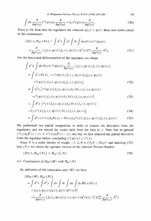
f du--'c~,q~(t)l~b(~(.) ) ~b(t,----- ~ OaVb(Tl(t))t~b(t ~ (50)

Since in the limit that the regulators are removed r/(s) _~ r/(t), these two terms cancel in the commutator,

[D(v),He,,(N)] m f d 3 x / d s / d t / d u N ( x ) v ° ( ~ 7 ( u ) )

8 8 ×Sr/a(u ) ( f~(x ,r / (s) ) f , , (x , rl(t)))~l'(s)T~![ - T/]. (51)

6rll' ( t ) '

For the functional differentiation of the regulators we obtain

f d3x f duN(x)v"(rl(.))~(f~(x, rt(s))f~,(x,~(t))) f d3x N(x) I - #'(rl(s) )f~, (x, rl(t) )O,,fE (x, rl(s ) )

-v"(rl(t) ) f~(x, rl(s) )O,,f~, (x, r/(t) )] (52)

= ./d3x [t/'(~7(s))fe(x, rl(s))a,,(N(x)f , ,(x, rl(t)))

+v°(~7(t) ) f~,(x, rI(t) )a,,( N(x) f~(x, rj(s) ))] (53)

~_ / d 3 x [c'"(x)f~(x, rl(s))O,,(N(x)f~,(x,r~(t)))

-c~,,(t,"(x)f~, (x, 'q(t) ) ) N(x)f~(x, rl(s) )] (54)

tx)c?,N(x) " -N(x)Oav"(x)) fe(x , rl(s))fe,(x, rI(t)). (55)

We performed two partial integrations in order to remove the derivative from the regulators, and we moved the vector field from the loop to x. Note that in general vO(y)O,,aB(x- y) 4= v"(x)4,a3(x- y), and that we first removed the partial derivative from the regulator before concluding v"(r/(s)) ~_ v"(x).

Since N is a scalar density of weight - 1, £,,N = v%,N - N4,v", and inserting (55) into (51) we obtain the operator version of the classical Poisson bracket,

[ D(v),Hee,( N) ] ~_ Hee,( E,N). (56)

4.3. Commutator of H6a, ( M) with HEe, ( N)

By definition of the constraints and (42) we have

[ H~a, (M), HEE, (N) l

× fa(x, rl(s) )fa,(x, rl(t) )il"( s)Ti( 6 6

, T i ]T~ [ 6rib ( × [ ~ (fe(y,~7(u))fe,(y, 71(v))iT~,(u)) i k v),T,k ]

264 B. Briigmann/Nuclear Phrsics B 474 (1996) 249-268

- ( M ~ N, 8 ~ e,81 ~ el). (57)

Functional differentiation of the tangent vector gives

r l t t ) dt f~(y, rl(t))T[)8~ (58)

t) ~ T k,st' d Tk s~' = ilc(t)3cfE(Y, rl( , ' , ~a -- re(Y, rl(t)) dt.t a"

(59)

The second term does not contribute to the commutator since

M(x) N(y)fa(x , rl(s) ) f a, (x, r/(t) )f~ (y, r/(t) )f~, (y, r/(c) )

- N ( x ) M ( y ) f ~ ( x , rl(s))fe,(x, rl(t))fa(y, rl(t))f~,(y, rl(v)) ~--0. (60)

Therefore, the functional differentiation of the tangent vector in the commutator gives

f d3x f d3y / d s / d t } d u M ( x ) N ( Y ) f a ( x , rl(s))f~'(X, rl(t))

×aaf~ (y, rl(t) ) f , , ( y, rl(u) )il~'( s)fl"( t)Tii[T[, 7'/] [ 6rib(u------- ~

- ( M +-* N, 8 ~-~ e,8' .-~ E'). (61)

To remove the partial derivative from the regulator, we perlbrm a partial integration in

y, and with approximations similar to (60) ,

} d3 x / d3 y M(x)N(y) f,s(x, rl(s) ) f,~,(x, rl(t) )SafE(y, rl(t) ) fE'(Y,~7(u) )

- f d3x f d3yN(x)M(y)f (x,v(s))f ,(x, ~--fd-~xfd3yo~,,(x)fa(x,~(s))f~,(x,~(t))f,(y, rl(t))f~,(y,~(u))

(62)

(63) _~ -oo,, (,q ( u ) ) f a ( r l ( u ) , rl(s) ) fdr l (u) , rl(t) ),

where

~o,(x) = M(x)&N(x) - N(x)O,M(x). (64)

(w,, is a covector density of weight - 2 , and w,f~f~ has weight 0.) In (63) we integrate over x and y keeping terms to leading order. Note that already in the definition

(30) of the Hamiltonian constraint one of the regulators can be removed without any renormalization, say f~, (x, "r/(t) ) ~ 8 s (x, r/(t) ). But after integrating over x, it is then

not quite clear how to perform the necessary partial integrations in the commutator

algebra. Functional differentiation of the regulators in the commutator (57) leads directly to

partial derivatives of regulators, which can be removed analogously, and we obtain for

B. Bri~'gmann/Nuclear Physics B 474 (1996) 249-268 265

the full commutator (after appropriate renaming of integration variables and contracted indices)

[ Haa, ( m ) , Ha~, (N) ]

( × [Tk,T;!]T/[fi~,(u),T,~] + T~JtTk,g][fi--~T~u),Tk]

) +T;{Tk[[ fir/b(u------- ~, T,~],T/{] . (65)

A priori it is not obvious how the right-hand side of the classical Poisson bracket (3) , D(gabwb), should be represented in the loop representation because of the operator product of the metric with the generator of diffeomorphisms. Comparing the above with the loop operators for the diffeomorphism constraint (29) and the metric (31 ), a natural guess is that the reroutings in (65) combine to T~iTiif/sr/b(u). This is indeed the case.

The first two terms in (65) cancel since with (27),

6 fi [Tk' T~i]Tii[ 8r/"(u~---)-' 7k] + Ti{[Tk' T[] [ 8 r / " (u ) ' T~]

,cikJTiTJTk 4- ~:ikJTJTiTk = [ ~ , ~ - ~ - , - u - - - i - , - . ] (66)

= 0, (67)

Note that the cancellation does not depend on whether 6/Sr/b(u) is located at u - or II ÷.

However, the one remaining term cannot be simplified using the SU(2) commutator for the insertion operators, because resolving the order of the insertions puts the derivative between the insertion operators,

fi T,~ ], T/~ ] = 8 S Tj ar/,,(,,------7' T'fT'I - " '

_ T j 8 T~ + T I T~ /, 3 " ar/~' ( u - ~ - fir/ (u+) " (68)

Of course, there are other identities to work with, but let us first consider the situation in the connection representation, i.e. g,[r/] = trU, 7 and 6/Srll'(u) = ilb(u)Fie(r/(u) )T'. Then the rerouting simplifies according to

T;(T) [ [T,'I, T,~ ] ,T,I] = T~(T) eik' eti'"T,', '' = T~T/T,I T~'T/T,',. (69)

The important observation is that this result cannot be transformed back to a functional derivative and some reroutings in the loop representation because in the first term F,i,/,(r/(u)) is contracted into an insertion at s, not u. In the limit that the regulators are removed in (65) , we have r/(u) ~_ r / (s) , and


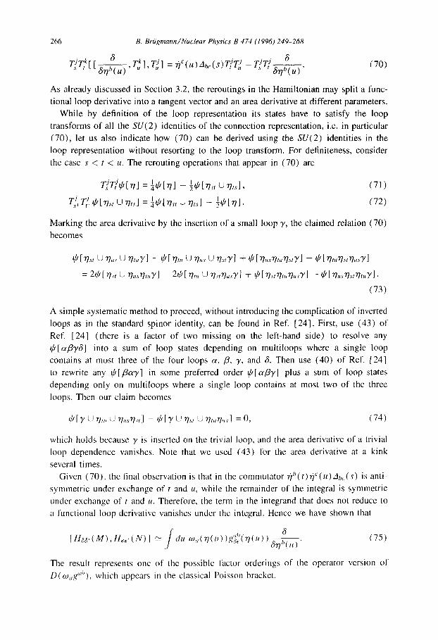
T i ( T t ~ [ [ 3_ ,T~ ] T~] = i l C ( u ) A b ~ ( s ) T / T J - T:/T: / fi • 6~Tb(U) , s t fi~Tb(u ) . (70)

As already discussed in Section 3.2, the reroutings in the Hamiltonian may split a functional loop derivative into a tangent vector and an area derivative at different parameters.

While by definition of the loop representation its states have to satisfy the loop

transforms of all the SU(2) identities of the connection representation, i.e. in particular (70), let us also indicate how (70) can be derived using the SU(2) identities in the

loop representation without resorting to the loop transform. For definiteness, consider

the case s < t < u. The rerouting operations that appear in (70) are

T:,?T[~ [ r / ] = ¼¢[ ' r / ] - ½ ,d.,[r/.,., U r/ ts] , ( 71 )

T:(, T/, ~['r/.,., U "q,.,.] = ¼0[~7.,, U r/,.,] - ½,d,[r/]. ( 72 )

Marking the area derivative by the insertion of a small loop y, the claimed relation (70)

becomes

¢ , [ m , u ~,,,,. u ~, , ,y] - ¢,[~,,, u ~,,,. u m. ,y ] + #-,[~,,.,.v,,,m,y] - ¢ , [~ , , ,m,~ , . -y ]

= 2~ It/,., U r h , . , ~ . , y J - 2~[~,,, , U %.,'r/..,.y] + d.,[ r/.,,r/t,'rh,.,.y] - ¢[~..~r/.,,,r/tHy].

(73)

A simple systematic method to proceed, without introducing the complication of inverted

loops as in the standard spinor identity, can be found in Ref. [24]. First, use (43) of

Ref. [24] (there is a factor of two missing on the left-hand side) to resolve any ¢[otf ly f i] into a sum of loop states depending on multiloops where a single loop contains at most three of the four loops a, /3, y, and & Then use (40) of Ref. [24]

to rewrite any gt[flcey] in some preferred order ~[a /3y] plus a sum of loop states depending only on multiloops where a single loop contains at most two of the three

loops. Then our claim becomes

d t [ y U "r/,,, O r / , j / . , , ] - ~ [ 7 U "r/.,, U "q.,r/l,,,.] = 0, (74 )

which holds because y is inserted on the trivial loop, and the area derivative of a trivial loop dependence vanishes. Note that we used (43) for the area derivative at a kink

several times. Given (70), the final observation is that in the commutator ¢lh( t ) i I"(u)At , r ( s ) is anti-

symmetric under exchange of t and u, while the remainder of the integral is symmetric

under exchange of t and u. Therefore, the term in the integrand that does not reduce to

a functional loop derivative vanishes under the integral. Hence we have shown that

[ H ~ s , ( M ) , H E E , ( N ) ] / ' d u w . (~7(u )" ""' ) ~r/,~( ~-- Jgs~(~7(tt) u) " (75)

The result represents one of the possible factor orderings of the operator version of

D(~o,g":') , which appears in the classical Poisson bracket.

B. Briigmann/Nuclear Physics B 474 (1996) 249-268 267

5. Conclusion

We have confirmed the result of Ref. [ 14] that the constraint algebra of 3+1 quantum gravity in the loop representation formally closes. There are two reasons for the com- parative simplicity of our calculation. We were able to cast the Hamiltonian constraint into a form involving only functional loop derivatives instead of area derivatives, and we found a simple way to separate the rerouting operations from the other parts of the

calculation. One direction for further research is to analyze the point-splitting regularization in

more detail, in particular to analyze the next-to-leading order terms [ 19]. This appears to be necessary if one decides to take the point-splitting regularization seriously, since

one cannot remove the regulators in the definition of the constraints before computing their algebra without running into inconsistencies related to the background dependence

of the regularization (also see the comment following (64)) . Turning this observation around, we avoid anomalous background-dependent terms in the constraint algebra by

postponing the removal of the regulators until the algebra is computed. A related point is that if we remove the regulator, the Hamiltonian constraint consists

of discrete sums over kinks and intersections (no integrals involved) and integrals along

the loops for the acceleration terms [6,8,19]. The acceleration terms in a sense spoil

the simple picture that the Hamiitonian constraint only acts on intersections, which are invariant under diffeomorphisms, although the background is present as an angle dependence, and the acceleration terms depend on the background since they contain second

derivatives of the loop, #" ( s ) . Sometimes one would like to argue away the acceleration terms, but notice that in order to obtain the integral on the right-hand side of the com-

mutator of two Hamiltonians, (3), and as is also apparent from Section 4.3, it does not suffice to just consider the discrete sums corresponding to kinks and intersections. This

may still be consistent with a diffeomorphism-invariant scheme like that of Ref. [ 11 ], in which acceleration terms do not appear, since, as we discussed in the introduction,

(3) is no longer relevant. As a final remark, note that the rigorous framework based on diffeomorphism-invariant

measures [9,12,16] is well adapted to the generators of diffeomorphisms, but has problems with the area derivatives appearing in the Hamiltonian constraint. Therefore it may be worthwhile to examine our form of the Hamiltonian constraint (30) in that setting.

Acknowledgements

It is a pleasure to thank Abhay Ashtekar, John Baez, Roumen Borissov, Renate Loll

and Carlo Rovelli for helpful discussions.

References

I 1 I R. Jackiw, Quantum modflications to the Wheeler DeWitt equation, gr-qc/9506037.


12l C. Rovelli and L. Smolin, Phys. Rev. Lett. 61 (1988) 1155; Nucl. Phys. B 331 (1990) 80. 131 A. Ashtekar, Phys. Rev. Lett. 57 (1986) 2244. 141 A. Ashtekar, Lectures on non-perturbative canonical gravity (World Scientific, Singapore, 1991). 15] B. Br~igmann, Loop representations, in Canonical Gravity: From Classical to Quantum, ed. J. Ehlers and

H. Friedrich (Springer, Berlin, 1994) p. 213. 16[ M. Blencowe, Nucl. Phys. B 341 (1990) 213. [71 R. Gambini, Phys. Lett. B 255 (1991) 180. 18] B. Briigmannand J. Pullin, Nucl. Phys. B 390 (1993) 399. 191 A. Ashtekar, J. Lewandowski, D. Marolf, J. Mour~o and T. Thiemann, J. Math. Phys. 36 (1995) 6456.

II01 B. Briigmann, Ph.D. Thesis, Syracuse University, 1993. [ 11 I C. Rovelli and L. Smolin, Phys. Rev. Lett. 72 (1994) 446. 112] A. Ashtekar and J. Lewandowski, Representation theory of analytic holonomy C* algebras, in: Knots

and Quantum Gravity, ed. J. Baez (Oxford University Press, Oxford, 1994). ] 131 T. Thiemann, Reality conditions inducing transforms for quantum gauge field theory and quantum

gravity, gr-qc/9511057; A. Ashtekar, A generalized Wick transform for gravity, gr-qc/9511083,

[ 141 R. Gambini, A. Garat and J. Pullin, The constraint algebra of quantum gravity in the loop representation, gr-qc/9404059.

115] R. Gambini and J. Pullin, Loops, knots, gauge theories and quantum gravity (Cambridge University Press, in press).

1161 J. Baez, Diffeomorphism invariant measures on the space of connections modulo gauge transformations, in Proc. Conf. on Quantum Topology, ed. D. Yetter (World Scientific, Singapore, 1994).

117] R. Loll, Nucl. Phys. B 444 (1995) 619; Phys. Rev. Lett. 75 (1995) 3048. 1181 B. BrOgmann, R. Gambini and J. Pullin, Phys. Rev. Lett. 68 (1992) 431. The tricky part is that one

has to commute the limit which leads to diffeomorphism invariance with the limit defining the area derivative of the Hamiltonian constraint. A similar interchange of limits appears for example also in S. Major and L. Smolin, Quantum deformation of quantum gravity, gr-qc/9512020.

[ 191 R. Borissov, Regularization of the Harailtonian constraint and the closure of the constraint algebra, gr-qc/9411038.

1201 N. Tsamis and R. Woodard, Phys. Rev. D 36 (1987) 3691. 1211 J. Friedman and 1. Jack, Phys. Rev. D 37 (1987) 3495. 122] B. Briigmann, R. Gambini and J. Pullin, Nuc[. Phys. B 385 (1992) 587. [23J J. Tavares, Int. J. Mod. Phys. A 9 (1994) 4511. 1241 B. BriJgmann and J. Pullin, Nucl. Phys. B 363 (1991) 221.

on the constraint algebra of quantum gravity in the loop...

Documents