on the capacitated step-fixed charge transportation and

Proceedings of the International Conference on Industrial Engineering and Operations Management

Pretoria / Johannesburg, South Africa, October 29 – November 1, 2018

© IEOM Society International

On The Capacitated Step-Fixed Charge Transportation

And Facility Location Problem:

A Local Search Heuristic

Gbeminiyi John Oyewole Department of Industrial and Systems Engineering,

University of Pretoria,

Pretoria 0002, South Africa

[email protected]

Olufemi Adetunji Department of Industrial and Systems Engineering,

University of Pretoria,

Pretoria 0002, South Africa

[email protected]

Abstract

Facility location, route selection and load consolidation are integrated distribution planning problems.

These three decisions are of long, medium and short terms respectively. In all these three decision

areas, there could be economy or diseconomy of scale involved. Of particular interests are models

with single and multiple price breaks. This paper studies a heuristic based on Linear Programming

(LP) relaxation for solving this integrated distribution problem. The solution approach utilizes simple

transportation problems which other known heuristics in literature have also employed. However, the

solution approach ensures that a reduced number of transportation problems are solved. A numerical

example is presented to ensure the comprehension of the workings of the solution method. Results

obtained for the first set of computational problems show little or no statistical difference in means

while the second set of problems had the modified u-v method final solution better than the other

methods considered. Although computation studies on a small scale was done to compare the

performance of the heuristic with the solution provided by standard optimization environment of Java

Eclipse and CPLEX, large problem sizes still proof necessary to compare the runtime and objective

value of each solution method.

Keywords: Facility location, step-fixed charge, linearization, transportation problem

1. Introduction

The classical transportation model and the solution tableau have been used to model and solve many real life

distribution problems. In the classic transportation problem, it is assumed that there are no fixed charges and

there is no economy (or diseconomy) of scale. The limitation of this assumption is well understood and many

models relaxing these two assumptions have been published by diverse authors. This has resulted in other sub-

classes of the transportation model such as the Fixed Charge Transportation Problem (FCTP), in which only the

“no fixed charge” assumption is relaxed, and the Step-Fixed Charge Transportation Problem (SFCTP) where

both assumptions are relaxed.

The FCTP and SFCTP, are integrated distribution problems of the simple transportation tableau problem with

fixed charges and has attracted a lot of research interests. Models and solutions presented by Gray (1971) ,

Sandrock (1988), Adlakha and Kowalski (2003), Kowalski and Lev (2008), Adlakha et al. (2007) show that the

fixed charges could occur either at the source or along the routes. Adlakha and Kowalski (2003), described the

FCTP as one in which there is a variable cost and a fixed cost incurred for opening a transportation route with a

shipment greater than zero. The SFCTP however, has more than one fixed charge being incurred along the route

as described by Sanei et al. (2017). Research in the field of the SFCTP is growing as indicated by Altassan et al.

227

mailto:[email protected]

[email protected]




(2013) and El-Sherbiny and Alhamali (2013) with new problem type models and solution techniques being

continually developed.

Facility location models on the other hand, as described by Ray (1966) and Sá (1969) have evolved from the

simple plant un-capacitated models to the complex capacitated models with various integrated transportation

and inventory models such as in Huang et al. (2015) and Carlo et al. (2017) . The field of Facility Location

Problems (FLP) over the years have centred around choosing a set of locations (Plants, warehouses, depots etc.)

from other potential locations where the fixed location cost is usually used as part of the model parameters in

selecting the best locations to satisfy the model objective and constraints.

The integrated Step-Fixed Charge Transportation Problem and Facility Location Problem which we have

called SFCTLP was indirectly modeled by Correia et al. (2010) as a capacitated transportation model problem

with modular distribution costs where the step-fixed charges were shown as a number of modules in a link from

source to destination. Furthermore, they presented a reformulated model with new valid inequalities to

strengthen their linear programming relaxation solution. Christensen (2013) also discussed the SFCTLP and

referred to it as Capacitated Facility Location Problem with Piecewise Linear Transportation Cost (CFLP with

PLTC).

As seen in literature and also noted by Christensen (2013), good number of solutions have been put forward in

solving separately the two main aspects of SFCLTP which are the FLP and SFCTP respectively. In the case of

SFCTP, Kowalski and Lev (2008) and Altassan et al. (2013) adapted the linear programming relaxation method

of Balinski (1961) to find an initial solution and Kowalski and Lev (2008) subsequently used a structured

perturbation logic to arrive at an improved solution. El-Sherbiny and Alhamali (2013) presented a metaheuristic

solution method to solve the SFCTP. Kim and Pardalos (2000) presented the dynamic slope scaling heuristic

based on LP relaxation to solve the Fixed Charge Network Flow problem (FCNFP) with similarity in modelling

to FCTP, and a possible extension to solve SFCTP. Furthermore, Christensen and Labbé (2015) provided a

branch and cut solution method based on LP relaxations and compared the efficiency of their solution methods

with a standard Mixed Integer Linear Programming (MILP) solver method such as CPLEX. Some solutions to

the SFCTP have revolved around introducing strong inequalities for LP relaxation. These have been noted by

Croxton et al. (2007) in their SFCTP called multi-commodity network design problem as strong and binding

constraints. They concluded that the LP relaxations approximate the objective function when the total flow is on

each arc or route.

Solutions presented in literature for solving both simple FLPs and integrated FLPs have been through the use of

the exact methods such as branch and bound , cutting plane algorithms to the use of LP based heuristics,

Lagrangian relaxation heuristics , local search heuristics and metaheuristics as noted by Wu et al. (2017). In

solving the CFLP with PLTC, Christensen (2013) described the problem as NP-hard. He suggested valid in-

equalities for strengthening the linear programming relaxation and also presented a lagrangian relaxation

heuristic solution and compared the efficiency of the solution obtained with a standard MILP solver such as

CPLEX.

In this paper, we study the SFCLTP which has been described to be NP-hard and consequently develop an LP

based relaxation heuristic to solve the problem. We have considered two fixed charges in the route without loss

of generality. Furthermore we introduce more valid inequality and equality approximations to the model of

Christensen (2013). The LP relaxation heuristic we developed adapts the principle of linearized cost by Kim

and Pardalos (2000). Our solution begins with some violation of the supply capacities but through the minimum

total demand flow cost from a source to all destinations for feasible locations, we develop a simple

transportation problem that ensures the demand and supply constraints are met. We also present the results of

some problem instances solved based on the LP heuristic in comparison to those obtained from using the

CPLEX concert technology with the code written in Java.

2 Base Model Formulation for SFCLTP

The one stage or two echelon SFCTP and SFCLTP are described as 𝑚 suppliers and 𝑛 demand point

distribution problems, where 𝑚 connotes the number of sources (factories or distribution centers) and the 𝑛

refers to the number of customers, demand or sink points. There are capacities and demand for each sources or

locations and demand point respectively over a time period, usually annual. The 𝑚 suppliers incur a unit

transportation cost per unit distance and there are more than one fixed charge in the route, link or arc depending

on the number of break points in the transportation routes. The SFCLTP, further consists of fixed location costs

attached to several potential locations to which the cheapest locations that satisfies the problem constraints are

228




to be selected. Christensen (2013) presented a mathematical model for the Multi Choice Model (MCM) of the

CFLP with PLC which forms a base for our SFCLTP and represented below:

Min Z =

∑ ∑ ∑(𝑐𝑖𝑗𝑙𝑥𝑖𝑗𝑙 + 𝑔𝑖𝑗𝑙𝑣𝑖𝑗𝑙) + ∑ 𝐹𝑖 𝑦𝑖

𝑛

𝑖=1

𝑞

𝑙=1

𝑚

𝑗=1

𝑛

𝑖=1

(1)

Subject to (constraints):

∑ ∑ 𝑥𝑖𝑗𝑙

𝑞

𝑙=1

𝑛

𝑖=1

= 𝐷𝑗 ∀ 𝑗 (2)

∑ 𝑣𝑖𝑗𝑙

𝑞

𝑙=1

≤ 1 ∀ (𝑖, 𝑗 ) (3)

∑ ∑ 𝑥𝑖𝑗𝑟

𝑞

𝑙=1

𝑚

𝑗=1

≤ 𝑆𝑖𝑦𝑖 ∀ 𝑖 (4)

𝑥𝑖𝑗𝑙 ≤ 𝐿𝑖𝑗𝑙 𝑣𝑖𝑗𝑙 ∀ (𝑖, 𝑗, 𝑙 ) (5)

𝑥𝑖𝑗𝑙 ≥ 𝐿𝑖𝑗𝑙 𝑣𝑖𝑗𝑙 ∀ (𝑖, 𝑗, 𝑙 ) (6)

𝑥𝑖𝑗𝑙 ≥ 0 (7)

𝑦𝑖 ∈ { 0,1} ∀ 𝑖 (8)

𝑣𝑖𝑗𝑙 ∈ { 0,1} ∀ (𝑖, 𝑗, 𝑙 ) (9)

Equation (1) is the total cost minimization objective function representing location and transportation cost.

Equation (2) represents the compulsory demand capacity. Equation (3) enforces one transportation mode

between each pair of source and destination. Equation (4) represents supply capacity not being exceeded.

Equation (5) ensures an upper bound on the load distribution, while Equation (6) enforces a lower bound on

distribution. Equation (7) refers to the non-negativity constraint while equation (8 and 9) refer to the binary

constraints.

3 Problem Structure And Formulation for SFCLTP

For the linearization and relaxation of our solution for the SFCLTP, a valid inequality constraint for the break

point as used in the work of Sanei et al. (2017) was introduced to the model of Christensen (2013) to further

strengthen the LP lower bound relaxation . Secondly, the Balinski (1961) method of binary variable relaxation

which Kowalski and Lev (2008) and Altassan et al. (2013) employed in relaxing their binary fixed charge

variables was also employed. This method uses some constraints in the problem to relax the binary constraints

in the cost objective term. Which is a general approach commonly employed for LP relaxations.

3.1 Model Assumption

We make the following assumptions in our model:

1. Deterministic input

2. One stage or Two echelon problem

3. Two step-fixed charge cost without loss of generality

4. Single period and single item distribution problem.

3.2 Model Parameters

𝑖 : Index for set of Sources (Plants, Warehouses etc.)

𝑗 : Index for set of Destinations (Customers, Warehouses, depots etc. )

𝑚 : Number of sources (or plants)

𝑛 : Number of destinations (or demand point)

𝑐𝑖𝑗 : Unit cost of shipment on route (𝑖, 𝑗)

𝑆𝑖 : Supply Capacity for Source 𝑖

229




𝐷𝑗 : Demand Capacity for Destination 𝑗

𝐻𝑖𝑗 : First level fixed cost

𝐼𝑖𝑗 : Second level fixed cost

𝐴𝑖𝑗 : Break point for selecting the route fixed charges

Decision variables

𝑥𝑖𝑗 : Allocations (or load distributions) along route (𝑖, 𝑗)

𝑦𝑖 : Location variable for plant or source (0 or 1) 𝑔𝑖𝑗 : Binary fixed charge variable before the break point

𝑧𝑖𝑗 : Binary fixed charge variable after the break point

Objective function of the Original Problem:

Minimize 𝑍𝑂 =

∑ ∑ 𝑐𝑖𝑗

𝑛

𝑗=1

𝑚

𝑖=1

𝑥𝑖𝑗 + ∑ 𝐹𝑖 𝑦𝑖

𝑚

𝑖=1

+ ∑ ∑ 𝐻𝑖𝑗

𝑛

𝑗=1

𝑚

𝑖=1

𝑔𝑖𝑗 + ∑ ∑ 𝐼𝑖𝑗 𝑧𝑖𝑗

𝑛

𝑗=1

𝑚

𝑖=1

(10)

Subject to (constraints):

∑ 𝑥𝑖𝑗

𝑛

𝑗=1

≤ 𝑆𝑖𝑦𝑖 ∀ 𝑖 = 1 … 𝑚 (11)

∑ 𝑥𝑖𝑗

𝑚

𝑖=1

= 𝐷𝑗 ∀ 𝑗 = 1 … 𝑛 (12)

∑ 𝑆𝑖𝑦𝑖

𝑚

𝑖=1

≥ ∑ 𝐷𝑗

𝑛

𝑗=1

∀ 𝑖 = 1 … 𝑚, ∀ 𝑗 = 1 … 𝑛 (13)

𝑥𝑖𝑗 ≤ 𝑀𝑖𝑗 𝑔𝑖𝑗 ∀ 𝑖 = 1 … 𝑚, ∀ 𝑗 = 1 … 𝑛 (14)

𝑥𝑖𝑗 − 𝐴𝑖𝑗 ≤ 𝑀𝑖𝑗𝑧𝑖𝑗 ∀ 𝑖 = 1 … 𝑚, ∀ 𝑗 = 1 … 𝑛 (15)

𝑥𝑖𝑗 ≥ 0 (16𝑎)

𝑦𝑖 = 0 𝑜𝑟 1 𝑧𝑖𝑗 = 0 𝑜𝑟 1 𝑔𝑖𝑗 = 0 𝑜𝑟 1 (16b)

𝑔𝑖𝑗 = {1 𝑥𝑖𝑗 > 0

0 𝑂𝑡ℎ𝑒𝑟𝑤𝑖𝑠𝑒 , 𝑧𝑖𝑗 = {

1 𝑥𝑖𝑗 > 𝐴𝑖𝑗

0 𝑂𝑡ℎ𝑒𝑟𝑤𝑖𝑠𝑒 (16c)

𝑀𝑖𝑗 = min( 𝑆𝑖 , 𝐷𝑗) ∀ 𝑖 = 1 … 𝑚, ∀ 𝑗 = 1 … 𝑛

Equation (10) is the objective function. The first term is a variable cost, the second term is the facility location

cost and third term is the route step-fixed charge cost. Equation (11) is the supply capacity constraint of each

location or sources which should not be exceeded. Equation (12) is the demand constraint of each customer

which must be met. Equation (13) is the aggregate constraint for supply and demand balance. Equation (14) is a

constraint that ensures that an upper bound on the load distribution before the break point is established.

Equation (15) is a constraint that ensures that a lower bound on the load distribution after the break point is

established. Equation (16a) refers to the non-negativity constraint while (16b) refer to the binary integer

constraints. Equation (16c) ensures the objective function selects the fixed charges based on the break points.

4 Solution Method

As indicated in earlier sections, the solution method presented in this work is based on linearizing the cost

objective function through the relaxation of some of the constraints. The relaxed constrains are used in objective

function to relax the location 𝑦𝑖 and the route fixed charge 𝑔𝑖𝑗 and 𝑧𝑖𝑗 variables. Figure 1 represents the

linearization cost structure of the objective function 𝑍𝑂 before and after linearization. The linearized model is

solved to optimality as the first transportation problem and a lower bound to the SFCLTP is obtained from the

result of the first transportation problem solution. The linearized cost solution obtained however may produce

some supply capacity infeasibilities at the sources, which have to be resolved before the desired solutions are

obtained. Our LP heuristic resolves the supply infeasibilities by identifying the combination of potential sources

that meet the demand. Using the linearized cost version of equation (10) and assuming total flow of all the

demand load from a source (𝑖) and all destinations(𝑗), we compute the total flow for each of the sources

(𝑖 = 1 … 𝑚). Croxton et al. (2007) suggested that the LP relaxation of the cost objective function would give an

230




𝑐𝑖𝑗 (𝑀𝑖𝑗 − 𝐴𝑖𝑗)

Total cost

approximation of the original problem with the “lower convex envelope”, when the total flow on each route is

used in computation.

Finally, Combination(s) of the sources (𝑖) that meet all the demand ∑ 𝐷𝑗𝑛𝑗=1 ∀ 𝑗 = 1 … 𝑛 with the least cost

combination using the linearized version of cost equation (10) is selected for the final transportation problem.

To solve the final transportation problem, we use the relaxed cost combination of 𝑐𝑖𝑗,𝐻𝑖𝑗 𝑎𝑛𝑑 𝐼𝑖𝑗 to determine

the final load distribution ( 𝑥𝑖𝑗) to be used in equation (1).

4.1 Linearized Cost Solution

The principle of linearized cost as used by Kim and Pardalos (2000) is adapted for the linearization to solve the

first transportation problem. We select the constraints (11), (14) and (15) respectively, place an equality upper

bound on them and use them in relaxing the fixed location cost and fixed charge variables 𝑦𝑖 , 𝑔𝑖𝑗 and 𝑧𝑖𝑗

respectively in the objective function equation (1).

The constraints given by (11), (14) and (15) are transformed respectively into

∑ 𝑥𝑖𝑗

𝑛

𝑗=1

= 𝑆𝑖𝑦𝑖 ∀ 𝑖 = 1 … 𝑚 ( 17 )

𝑥𝑖𝑗 𝑀𝑖𝑗⁄ = 𝑔𝑖𝑗 (18 )

(𝑥𝑖𝑗 − 𝐴𝑖𝑗)/ 𝑀𝑖𝑗 = 𝑧𝑖𝑗 ( 19 )

We substitute this equation (17) into the aggregate constraint of equation (13) above to obtain

∑ 𝑆𝑖(∑ 𝑥𝑖𝑗

𝑛𝑗=1

𝑆𝑖

𝑚

𝑖=1

) ≥ ∑ 𝐷𝑗

𝑛

𝑗=1

∀ 𝑖 = 1 … 𝑚, ∀ 𝑗 = 1 … 𝑛 (20)

Substituting equation (17) (18) and (19) into the objective function (equation (1)) and using the derived

equation (20) would give a linear programming problem model of the Original problem, given as :

Min 𝑍𝐿𝑃𝑂 =

∑(𝐹𝑖 ∑ 𝑥𝑖𝑗

𝑛𝑗=1

𝑆𝑖

𝑚

𝑖=1

) + ∑ ∑ 𝑐𝑖𝑗

𝑛

𝑗=1

𝑚

𝑖=1

𝑥𝑖𝑗 + ∑ ∑ 𝐻𝑖𝑗

𝑛

𝑗=1

𝑚

𝑖=1

𝑥𝑖𝑗

𝑀𝑖𝑗

+ ∑ ∑ 𝐼𝑖𝑗 𝑥𝑖𝑗 − 𝐴𝑖𝑗

𝑀𝑖𝑗

𝑛

𝑗=1

𝑚

𝑖=1

(21)

Quantity shipped

𝑐𝑖𝑗𝐴𝑖𝑗

𝐹𝑖

𝐼𝑖𝑗

𝐴𝑖𝑗

Figure 1. Adapted Linearization And Relaxation Structure For SFCLTP (Kowalski and Lev, 2008)

method

Step function objective

function

Linearization of fixed

charge binary and

location variable

𝐻𝑖𝑗

𝑀𝑖𝑗 𝑋𝑖𝑗

231




Subject to

∑ 𝑥𝑖𝑗

𝑚

𝑖=1

= 𝐷𝑗 ∀ 𝑗 = 1 … 𝑛 (22)

∑ 𝑆𝑖(∑ 𝑥𝑖𝑗

𝑛𝑗=1

𝑆𝑖

𝑚

𝑖=1

) ≥ ∑ 𝐷𝑗

𝑛

𝑗=1

∀ 𝑖 = 1 … 𝑚, ∀ 𝑗 = 1 … 𝑛 (23)

𝑥𝑖𝑗 ≥ 0 (24)

Equation (21) could also be restated as

𝑍𝐿𝑃0 =

∑(𝐹𝑖 ∑ 𝑥𝑖𝑗

𝑛𝑗=1

𝑆𝑖

𝑚

𝑖=1

) + ∑ ∑(𝑐𝑖𝑗

𝑛

𝑗=1

𝑚

𝑖=1

+𝐻𝑖𝑗

𝑀𝑖𝑗

+𝐼𝑖𝑗

𝑀𝑖𝑗

) 𝑥𝑖𝑗 − ∑ ∑ 𝐼𝑖𝑗 𝐴𝑖𝑗

𝑀𝑖𝑗

𝑛

𝑗=1

𝑚

𝑖=1

(25)

Equations(21) to (24) gives a linear programming problem which can be solved to optimality by any known

optimal linear programming solver.

4.2 Resolution of Linearization Infeasibility and Final Transportation Problem

We note that in the solution of the new relaxed model represented by equation (21) to (24), there could be

supply infeasibilities due to constraints (22) and (23) not strictly enforcing the supply requirements. We

however resolve these supply infeasibilities through our heuristic presented below:

Step 1: Select individuals or groups of potential sources ( 𝑖 ∈ 𝑚 ) such that

∑ 𝑆𝑖 𝑦𝑖𝑚𝑖=1 ≥ ∑ 𝐷𝑗

𝑛𝑗=1

Step 2: For the individuals or groups selected, Use equation (25) only to calculate 𝑍𝐿𝑃0𝑖 ∀ 𝑖 = 1 … 𝑚, where

the load distribution is given as 𝑥𝑖𝑗 ∶ 𝑥𝑖𝑗 = 𝐷𝑗 ∀ 𝑗 = 1 … 𝑛 .

(thus 𝑍𝐿𝑃01 is calculated using 𝑥11, 𝑥12, 𝑥13, … . . 𝑥1𝑛, )

Step 3: From the individuals or groups of 𝑖 ∈ 𝑚 selected in step 1, choose the minimum 𝑍𝐿𝑃0𝑖 or

combinations of 𝑍𝐿𝑃0𝑖 ( ∑ 𝑍𝐿𝑃0

𝑖𝑚𝑖 ) if groups are selected. We note that 𝑍𝐿𝑃0

𝑖 values could be positive or negative

depending on the problem parameters. This is evident by the third term in equation (25) which has the

possibility of making the equation negative. If the combinations of 𝑍𝐿𝑃0𝑖 are positive we select the minimum

value. However if the combinations of 𝑍𝐿𝑃0𝑖 are negative values we select the minimum absolute value.

Step 4: Solve the transportation problem created by using the sources selected in Step 4 and the relaxed cost

combination of ( 𝑐𝑖𝑗 +𝐻𝑖𝑗

𝑀𝑖𝑗+

𝐼𝑖𝑗

𝑀𝑖𝑗 ) subject to simple demand and supply constraints to obtain the load distribution

𝑥𝑖𝑗 for equation (1). The transportation problem to be solved is given as

𝑀𝑖𝑛 𝑍𝐹 =

∑ ∑(𝑐𝑖𝑗 +𝐻𝑖𝑗

𝑀𝑖𝑗

+𝐼𝑖𝑗

𝑀𝑖𝑗

)

𝑛

𝑗=1

𝑚

𝑖=1

𝑥𝑖𝑗 (26)

∑ 𝑥𝑖𝑗

𝑛

𝑗=1

≤ 𝑆𝑖𝑦𝑖 ∀ 𝑖 = 1 … 𝑚 (27)

∑ 𝑥𝑖𝑗

𝑚

𝑖=1

= 𝐷𝑗 ∀ 𝑗 = 1 … 𝑛 (28)

𝑥𝑖𝑗 ≥ 0 (29)

Step 5: Using the value of 𝑍𝑂, compare the load distribution 𝑥𝑖𝑗 obtained by solving the transportation model

given by equation (19) to (22) by any feasible approach such as the North-West Corner (NWC) method and

optimally using Simplex or the Modified u-v distribution method known as (Modi). Select the minimum 𝑍𝑂

obtained by the methods.

232




The Least Cost (LC) approach of solving the transportation problems ensures that maximum allocations are

made to the minimum relaxed cost position, while NWC approach ensures that allocations are made to the least

cost positions from a northwest corner of the transportation tableau. An optimal transportation cost solution

using the Modified u-v distribution method or Modi would perform dual variable (u and v) analysis and ensure

that 𝑚 + 𝑛 − 1 variable positions are occupied.

5. Numerical Solution Obtained

This section consists of the numerical computation done using a random problem size of (4× 4). Furthermore,

computation studies were done to further gain insight into the heuristic performance when compared to the

standard MILP solver such as CPLEX.

5.1 Numerical Example

In order to explain the workings of the LP based heuristic presented in section 4.2 above, we have adapted the

problem created by Kowalski and Lev (2008), represented the problem in Table (1) and (2) below and also

shown the solution below.

Table 1 : Supply, demand, location (set up) costs and unit cost parameters

. i

𝑆𝑖 𝐹𝑖 j = 1

2 3 4

𝑐𝑖𝑗

1

25 100 1 3 1 3

2

25 200 2 2 3 2

3

25 250 2 1 2 1

4

25 150 1 3 1 3

𝐷𝑗

10 30 20 15

Table 2 : Two tier fixed charges on route ( 𝒊, 𝒋)

i

𝐻𝑖𝑗 , 𝐼𝑖𝑗 𝐻𝑖𝑗 , 𝐼𝑖𝑗 𝐻𝑖𝑗 , 𝐼𝑖𝑗 𝐻𝑖𝑗 , 𝐼𝑖𝑗

1

10 ; 20 10 ; 10 10 ; 30 10 ; 10

2

10 ; 30 10 ; 20 10 ; 20 10 ; 20

3

10 ; 20 10 ; 30 10 ; 10 10 ; 30

4

10 ; 20 10 ; 10 10 ; 30 10 ; 10

j =1 2 3 4

The break point 𝐴𝑖𝑗 = 5 (𝑐𝑜𝑛𝑠𝑡𝑎𝑛𝑡 ) through route 𝑖, 𝑗

From section 4.1, using the linearized cost model represented by equation (21) to (24) we obtained the value of

𝑍𝐿𝑃𝑂 = 488.75

233




25

10 30 20 15

25 0 0 0 0

25 0 0 0 0

25 0 0 0 0

10 30 20 15

This clearly gives an infeasible solution as noted in section 4.

Step 1:

Using first step of the heuristic we obtain the combinations of locations to resolve the infeasible solution

obtained above i.e. (1,2,3), (1,2,4), (1,3,4), (2,3,4) and (1,2,3,4) as having ∑ 𝑆𝑖 𝑦𝑖𝑚𝑖=1 ≥ ∑ 𝐷𝑗

𝑛𝑗=1

However, it is clear that the combination of (1,2,3,4) would not be cost saving based on the extra fixed location

cost.

Step 2:

We compute objective value 𝑍𝐿𝑃0𝑖 for the four sources (no optimization done here) where :

𝑍𝐿𝑃01 is calculated using 𝑥11, 𝑥12, 𝑥13,𝑥14, = 488.75




The location (1,2,3) gives a sum of ( 488.75+794.5+867.75) = 2151

Similarly locations (1,2,4), (1,3,4), (2,3,4) gives 1921.82, 1995.07 and 2300.82 respectively.

Step3:

Since the combinations of 𝑍𝐿𝑃0𝑖 are positive , we select the minimum value. The location (1,2,4) possess the

minimum sum of linearized cost and thereby chosen.

Step 4:

We use the relaxed cost combination of 𝑐𝑖𝑗 +𝐻𝑖𝑗

𝑀𝑖𝑗+

𝐼𝑖𝑗

𝑀𝑖𝑗 given below as the new unit cost and solve the second

transportation problem given by equation (26) to (29) to obtain the final load distribution to be used to calculate

𝑍𝑂 in equation (10) above. The relaxed cost combination matrix is presented below.

4 3.8 3 5.166667

6 3.2 4.5 3.416667

5 2.6 3 2.166667

4 3.8 3 5.166667

Step 5:

The Load distribution obtained when Transportation problem (26) to (29) is solved optimally and using least

cost approach 𝑍𝐹 = 259.25 𝑎𝑛𝑑 𝑍𝑂 = 750 is presented below.

25

10 15 0 0

25 0 10 0 15

25 0 0 0 0

25 0 5 20 0

10 30 20 15

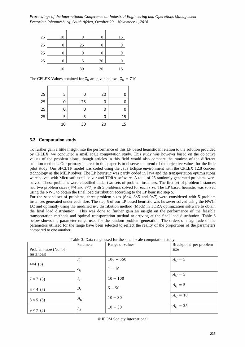
Using the Northwest corner approach when solving transportation problem (19) to (21) gives 𝑍𝐹 = 276.95 𝑎𝑛𝑑 𝑍𝑂 = 720 . This is shown below.

234




25

10 0 0 15

25 0 25 0 0

25 0 0 0 0

25 0 5 20 0

10 30 20 15

The CPLEX Values obtained for 𝑍𝑂 are given below. 𝑍𝑂 = 710

25

5 0 20 0

25 0 25 0 0

25 0 0 0 0

25 5 5 0 15

10 30 20 15

5.2 Computation study

To further gain a little insight into the performance of this LP based heuristic in relation to the solution provided

by CPLEX, we conducted a small scale computation study. This study was however based on the objective

values of the problem alone, though articles in this field would also compare the runtime of the different

solution methods. Our primary interest in this paper is to observe the trend of the objective values for the little

pilot study. Our SFCLTP model was coded using the Java Eclipse environment with the CPLEX 12.8 concert

technology as the MILP solver. The LP heuristic was partly coded in Java and the transportation optimizations

were solved with Microsoft excel solver and TORA software. A total of 25 randomly generated problems were

solved. These problems were classified under two sets of problem instances. The first set of problem instances

had two problem sizes (4×4 and 7×7) with 5 problems solved for each size. The LP based heuristic was solved

using the NWC to obtain the final load distribution according to the LP heuristic step 5.

For the second set of problems, three problem sizes (6×4, 8×5 and 9×7) were considered with 5 problem

instances generated under each size. The step 5 of our LP based heuristic was however solved using the NWC,

LC and optimally using the modified u-v distribution method (Modi) in TORA optimization software to obtain

the final load distribution. This was done to further gain an insight on the performance of the feasible

transportation methods and optimal transportation method at arriving at the final load distribution. Table 3

below shows the parameter range used for the random problem generation. The orders of magnitude of the

parameters utilized for the range have been selected to reflect the reality of the proportions of the parameters

compared to one another.

Table 3: Data range used for the small scale computation study

Problem size (No. of

Instances)

Parameter Range of values Breakpoint per problem

size

4×4 (5)

𝐹𝑖

𝑐𝑖𝑗

𝑆𝑖

𝐷𝑗

𝐻𝑖𝑗

𝐼𝑖𝑗

100 − 550

1 − 10

10 − 100

5 − 50

10 − 30

10 − 30

𝐴𝑖𝑗 = 5

7 × 7 (5)

𝐴𝑖𝑗 = 5

6 × 4 (5)

𝐴𝑖𝑗 = 5

8 × 5 (5)

𝐴𝑖𝑗 = 10

9 × 7 (5)

𝐴𝑖𝑗 = 25

235




The mean value, and the 5 different problem instances of the CPLEX and LP heuristic (using NWC solution)

generated are shown in Table 4 below. Also, the percentage mean difference have been included to show the

gap obtained from the CPLEX values. The larger the mean percentage, the poorer the results of the LP heuristic

in comparison to CPLEX values. Similarly to Table 4, Table 5 below presents the results obtained using the

northwest corner, least cost and modified u-v distribution method using only the mean values of the different 5

problem instances generated.

Table 4: First set of results obtained

Problem Size

Instance

No CPLEX (𝑍𝑂) LP heuristic

(𝑍𝑂) (NWC)

% mean

Difference

LP heuristic and

CPLEX

4×4

Mean values

1

2

3

4

5

( 𝑍𝑂̅̅̅̅ )

710

735

705

685

580

683

720

735

710

725

610

700

2.4%

7×7

Mean values

1

2

3

4

5

( 𝑍𝑂̅̅̅̅ )

1315

1425

1610

1910

1755

1603

1315

1480

1620

1920

1765

1620

1.0%

Table 5: Second set of results obtained

Problem

Size

Mean

CPLEX

(𝑍𝑂̅̅̅̅ ) Value

Mean

LP heuristic

(𝑍𝑂̅̅̅̅ )(NWC)

Mean

LP heuristic

(𝑍𝑂̅̅̅̅ )

(LC)

Mean

LP heuristic

(𝑍𝑂̅̅̅̅ ) (Modi)

% mean

difference

LP-NWC

and

CPLEX

% mean

difference

LP-LC and

CPLEX

% mean

difference

LP-Modi

and

CPLEX

6×4

1665 1915 1810 1731 15.01% 8.70% 3.96%

8×5

2471 2964 2514 2494 19.95% 1.74% 0.93%

9×7

2961 3392 3102 3015 14.56% 4.76% 1.82%

6. Discussion Of Solutions Obtained

From the results of the little computation study conducted it is easily seen that the CPLEX solution

outperformed the LP based heuristic as per the individual instances and mean values considered both in Tables 4

and 5. Results obtained for the first set of problems as per Table 4, shows the mean objective value gap

difference of 2.4% and 1.0% respectively. A quick analysis using the paired t-test of means for the (4×4)

problem size at 0.05 level of significance gave a p-value of 0.09130, showing there is not quite statistical

significance in the difference of the means obtained, while the second and larger problem size (7×7) gave a p-

value of 0.15440 showing no statistical significance in the difference of means. This further shows that the LP

heuristic may have the possibility of having very good solutions as the problem size increases. Furthermore we

observe that the NWC used to obtain the final distribution load for the LP heuristic had a good performance of

being close to 0% difference.

However, in the second set of problems as presented in Table 5, the NWC performance was consistently worse

when compared to LC and Modi. This shows that for certain problem structures the NWC could quickly obtain

good results. The LP based heuristic using the Modi and LC distributes the load using the minimum relaxed cost

of the problem parameters, while NWC does not. The LP-Modi in problem size (8×5) obtained the best mean

difference of 0.93%. Showing it has the likelihood of generating good results irrespective of problem size and

parameter structure.

236




Finally, the numerical problem considered showed the possibility of having near solutions to the CPLEX values

when a minimum value among the NWC, LC and Modi is used for the final load distribution of the LP based

heuristic.

7. Conclusion And Future Directions

In this paper, we considered the Facility Location (FL) and Step-Fixed Charge Transportation Problem

(SFCTP). A Linear Programming (LP) based heuristic was developed which was decomposed into two major

transportation problems. The relaxed objective function of the first transportation problem in equation (25) was

used in selecting the combinations of locations to be considered for the final transportation problem. In addition,

solving the first transportation problem could help in generating a good lower bound for other computation

methods such as Lagrange relaxations. A Numerical solution was presented to show the workings of the

heuristic while a small scale pilot computation study was done to gain a little insight into the heuristic

performance as regards the objective value obtained. Two sets of problem sizes were considered. The first set of

problem sizes was solved using the NWC method as a solution method for the final transportation problem. The

statistical results obtained showed a little or no significant differences in the mean values of the CPLEX solution

and the LP based heuristic with increase in problem size. However, the NWC method lagged behind the LC and

Modi methods for the second set of problem sizes. The Modi method for the final transportation problem was

superior in all the problem instances of the second set of problems. The optimal distribution pattern of the Modi

method (minimum cost) seemed to have a strong link to the good results obtained.

Conclusively, large scale computation study still have to be conducted to gain proper insight into the

performance of the heuristic under different parameter ranges and also due to the reason that exact methods

which may obtainable using the solution methods present in the CPLEX optimization studio could become

inefficient as the problem size increases. Also, comparing the runtimes of the different solution methods would

also need to be considered for an efficient study. Finally a comparative study between this LP based heuristic

and solution methods such as the lagrangian relaxation heuristic, metaheuristics such as genetic algorithm , tabu

search and hybrid solutions which uses both LP based relaxation and metaheuristics would be possible areas for

exploring.

References

Adlakha, V. & Kowalski, K. 2003. A Simple Heuristic For Solving Small Fixed-Charge Transportation Problems. Omega, 31, 205-211.

Adlakha, V., Kowalski, K., Vemuganti, R. R. & Lev, B. 2007. More-For-Less Algorithm For Fixed-Charge Transportation Problems. Omega, 35, 116-127.

Altassan, K. M., El-Sherbiny, M. M. & Sasidhar, B. 2013. Near Optimal Solution For The Step Fixed Charge Transportation Problem. Applied Mathematics & Information Sciences, 7, 661-669.

Balinski, M. L. 1961. Fixed‐Cost Transportation Problems. Naval Research Logistics (Nrl), 8, 41-54. Carlo, H. J., David, V. & Salvat, G. 2017. Transportation-Location Problem With Unknown Number Of

Facilities. Computers & Industrial Engineering. Christensen, T. 2013. Network Design Problems With Piecewise Linear Cost Functions, Institut For

Økonomi, Aarhus Universitet. Christensen, T. R. & Labbé, M. 2015. A Branch-Cut-And-Price Algorithm For The Piecewise Linear

Transportation Problem. European Journal Of Operational Research, 245, 645-655. Correia, I., Gouveia, L. & Saldanha-Da-Gama, F. 2010. Discretized Formulations For Capacitated

Location Problems With Modular Distribution Costs. European Journal Of Operational Research, 204, 237-244.

Croxton, K. L., Gendron, B. & Magnanti, T. L. 2007. Variable Disaggregation In Network Flow Problems With Piecewise Linear Costs. Operations Research, 55, 146-157.

El-Sherbiny, M. M. & Alhamali, R. M. 2013. A Hybrid Particle Swarm Algorithm With Artificial Immune Learning For Solving The Fixed Charge Transportation Problem. Computers & Industrial Engineering, 64, 610-620.

237




Gray, P. 1971. Technical Note—Exact Solution Of The Fixed-Charge Transportation Problem. Operations Research, 19, 1529-1538.

Huang, S., Wang, Q., Batta, R. & Nagi, R. 2015. An Integrated Model For Site Selection And Space Determination Of Warehouses. Computers & Operations Research, 62, 169-176.

Kim, D. & Pardalos, P. M. 2000. Dynamic Slope Scaling And Trust Interval Techniques For Solving Concave Piecewise Linear Network Flow Problems. Networks: An International Journal, 35, 216-222.

Kowalski, K. & Lev, B. 2008. On Step Fixed-Charge Transportation Problem. Omega, 36, 913-917. Ray, M. A. E. A. T. L. 1966. A Branch-Bound Algorithm For Plant Location. Sá, G. 1969. Branch-And-Bound And Approximate Solutions To The Capacitated Plant-Location

Problem. Operations Research, 17, 1005-1016. Sandrock, K. 1988. A Simple Algorithm For Solving Small, Fixed-Charge Transportation Problems.

Journal Of The Operational Research Society, 39, 467-475. Sanei, M., Mahmoodirad, A., Niroomand, S., Jamalian, A. & Gelareh, S. 2017. Step Fixed-Charge Solid

Transportation Problem: A Lagrangian Relaxation Heuristic Approach. Computational And Applied Mathematics, 36, 1217-1237.

Wu, T., Chu, F., Yang, Z., Zhou, Z. & Zhou, W. 2017. Lagrangean Relaxation And Hybrid Simulated Annealing Tabu Search Procedure For A Two-Echelon Capacitated Facility Location Problem With Plant Size Selection. International Journal Of Production Research, 55, 2540-2555.

Biographies

Gbeminiyi John Oyewole : Is currently a doctoral student in the Department of Industrial and Systems

Engineering at the University of Pretoria, South Africa. He obtained his Master’s degree in Industrial and

Production Engineering at the University of Ibadan, Nigeria. He has worked in field of Logistics, transportation

and as a supply chain officer at the Candel Agrochemical Plant in Lagos Nigeria. He is also an UNLEASH

award winner in the category of sustainable production and consumption, whose team was able to design

sustainable packaging materials for transportation using pallets. His research interests are in Facility location

problems, applied optimization, operations research, supply chain and engineering Designs.

Olufemi Adetunji: is currently a senior lecturer at the Department of Industrial and Systems Engineering at

the University of Pretoria, South Africa. He obtained his PhD at the same University. He has performed various

research work with National Research Foundation (NRF) South Africa and with other leading governmental and

private agencies within South Africa. He has also published a lot of articles in leading local and International

Journals. His research Interests are in Supply Chain design and Engineering , Lean Manufacturing and applied

optimization

238

on the capacitated step-fixed charge transportation and

Documents