On some basic results by application of the CZF method.

Elio Conte(1,2), Maria Pieralice(1) , Vincenza Laterza (1), Antonella Losurdo(1), Sergio Conte(1)

Antonio Federici (2) and

Alessandro Giuliani (3)

(1) School of Advanced International Studies for Applied Theoretical and non Linear Methodologies in Physics. Bari-Italy(2) Department of Pharmacology and Human Physiology, TIRES-Center for Innovative Technologies for Signal

Detection and Processing, University of Bari, Italy;

(3) Istituto Superiore di Sanità, Viale Regina Elena 299, 0016, Rome, Italy

Introduction.The autonomic nervous system (ANS) regulates internal organs and circulation dynamics. The term ‘autonomic’ is related to the fact that we retain that such regulation happens without any consciousness so that the body reaches an homeostatic (or better homeorhetic as proposed by Conrad Waddington to put the accent to the dynamic character of equilibrium) balance following ‘its own rules’ and so contrasting the influences arising from a mainly stochastic environment. Heart Rate Variability (HRV) must be considered to represent the most privileged observatory of ANS given the crucial role of having a blood flux consistent with the body needs, this regulation of blood flux entity is achieved by the variation in the periods of subsequent contraction/relaxation acts of heart muscle.The concept of sympathovagal balance in HRV refers to the autonomic state resulting from sympathetic and parasympathetic influences, i.e. ‘mainly activating’ and ‘mainly inactivating’ drives. During the last three decades, numerous studies have shown that abnormalities in the sympathovagal balance are related to different diseases [TaskForce 1996].Experimental studies have shown significant relations between ANS and cardiovascular diseases [TaskForce 1996, Acharya et al. 2006]. It has been observed that there is a relation between the risk of developing a lethal cardiac arrhythmia and signs of either increased sympathetic activity or decreased parasympathetic activity [TaskForce 1996, Stein et al. 1994]. Predominance of sympathetic activity and reduced parasympathetic cardiac control have been seen in patients with acute myocardial infarction [Ravenswaaij-Arts et al. 1993]. Moreover, congestive heart failure patients show alterations of the sympathovagal balance. The general approach points to a sympathetic overdrive rather than a parasympathetic withdrawal in such patients. An altered sympathovagal balance is also identified in patients after cardiovascular surgery and it has been related to myocardial ischemic episodes in patients who have undergone coronary artery bypass grafting [TaskForce 1996]. As a complication of diabetes mellitus, autonomic neuropathy occurs and this often affects the cardiac autonomic function as well. Diabetic neuropathy is characterized by early and widespread neuronal degeneration of small sympathetic and parasympathetic nerve fibres [Zipes & Jalife 2004( Ravenswaaij-Arts et al. 1993]). Patients with cervical and high thoracic spinal cord lesions also have autonomic abnormalities that affect the heart. In these patients some autonomic pathways are severed, but baroreceptor afferents and parasympathetic efferents of the ANS are intact. This causes a reduced ability to regulate the cardiac activity [Malik 1998].In the last few years , HRV analysis has shown increasing interest also in psychophysiology.

Higher HRV is linked with better physical and emotional health overall and has been shown to reduce risk for stress-related illness, such as cardiac problems, asthma, and diabetes, moreover a decrease in HRV was observed to be strictly related to aging even in normal subjects [A. Colosimo, A. Giuliani, A.M. Mancini, G. Piccirillo, V. Marigliano (1997) Estimating a cardiac age by means of Heart Rate Variability (HRV). Am. Journ. Physiol. (273) (Heart.Circ.Phy. 42): H1841-H1847, Giuliani A., G.Piccirillo, V.Marigliano, A.Colosimo (1998) A Non-linear Explanation for Aging Induced Changes in Heartbeat Dynamics. Am.Journ. Physiol. (Heart.Circ.Physiol. 275): H1455-H1461.]Studies have shown that training HRV can improve physical, mental, and emotional stability. Positive outcomes include improved cognitive abilities and mental clarity, greater emotional balance, enhanced creativity.HRV values are in turn influenced by the psychophysiological state of the individual [S.Koelesch et al. 2007,J.F. Thayer et al 1998,Yeragani 1991. In general, each subject shows a baseline (averaged) value of heart rate variability and sympathetic activation. These baseline values undergo relevant (around 30%) changes in response to routine psychological environmental solicitations along the day It is also possible to modify the HRV by means of suitable psychological techniques. This modifications can be stabilized with learning. There are two main ways for such ‘externally induced HRV changes: the first is based on somatic techniques (breathing, massage, relaxation, movement) and brings the patient towards an (at least subjectively) increased wellbeing state. The second way is based on psychological techniques and consists in a work on the deep consciousness and on the personality of the patient. Growing evidence suggests that alterations in autonomic function contribute to the pathophysiology of panic disorder (PD). The risk of adverse clinical cardiac events is increased in patients with panic disorder (PD). Autonomic nervous system (ANS) dysfunction and reduced heart rate variability (HRV) have been reported in a wide variety of psychiatric disorders. Some authors recorded cardiac activity and assessed HRV in acutely hospitalized manic bipolar (BD) and schizophrenia (SCZ) patients. Autonomic dysregulation is associated with more severe psychiatric symptoms, suggesting HRV dysfunction , [B. Henry 2009, Yeragani 1991]It is known that autonomic nervous activities change in correspondence with sleep stages. However,the characteristics of continuous fluctuations in nocturnal autonomic nerve tone have not been clarified in detail. Autonomic dysfunction has been the target of numerous investigations and has been linked to generalized anxiety disorder, panic disorder, and depression. Symptoms of depression often are accompanied by ANS abnormalities, including reductions in HRV, vagus nerve activity, and baroreflex sensitivity. Animal studies exploring the specific ANS mechanisms of depression by using the chronic mild stress rodent model of depression found that exposure to chronic stress decreased HRV and elevated sympathetic tone to the heart. It is of great interest also the application in HRV Biofeedback Training for Depression

In conclusion: in all HRV is a very important marker of autonomic activity and thus a privileged observatory for a lot of disease conditions, some of these conditions are very elusive and practically impossible to detect with reliable diagnosis methods. This justifies the interst in the development of analysis methods of HRV that could increase the sensitivity of diagnosis methods in different pathology fields.

The methodology for HRV

During the last decades different methods have been applied to assess the autonomic activity; these include for example cardiovascular reflex tests and biochemical tests [Ravits 1997]. In recent years,

noninvasive techniques based on electrocardiographic recordings have been used as markers of cardiac autonomic tone; Among these, heart rate variability (HRV) is the most widely used and evaluated [TaskForce 1996].The ANS regulates the heart rate; increased sympathetic activity causes acceleration whereas increased parasympathetic activity causes deceleration of the heart rate [Guyton & Hall 2006], which is the reason why HRV is used as a marker of autonomic activity. The increasing diffusion of HRV as a method to measure autonomic activity since the 70’s and a lack of method standardization combined with a continuous introduction of new HRV measures lead to the formation of a task force of the European Society of Cardiology and The North American Society of Pacing and Electrophysiology in 1996. The task force established standards of measurement, physiological interpretation, and clinical use of HRV [TaskForce 1996].In order to quantify HRV, the intervals between consecutive beats originating in the SA node, also called normal to normal intervals (NN intervals), must be found in the electrocardiogram (ECG). The analysis of HRV must satisfy four conditions:1) a satisfactory signal-to-noise ratio of the ECG is necessary to identify the each beat properly.2) the digital sampling must be regular and robust to identify a fiducial point for each beat,.3) morphology and rhythm characteristics for each beat must be classified to distinguish between

beats originating in the sinus node and ectopic beats. 4) only beats originating in the sinus node should be considered for the HRV analysis [Zipes &

Jalife 2004].

Two main approaches have been used to measure the HRV; time domain analysis and frequency domain analysis. Besides these, nonlinear analysis is an emerging field within the analysis of HRV.

Frequency Domain Analysis

The frequency domain measures are based on a transform of the series of subsequent registered RR intervals into the frequency domain. The series can be represented in two ways; as the RR intervals versus the beat number, as a discrete event series where the Ri-Ri−1 interval is plotted versus the time of occurrence of Ri. While Frequency Domain Analyses have a time honoured tradition in the study of time series in any scientific fields, nevertheless they show some evident limitations as the particular case of HRV. RR series can be considered as irregularly sampled signal : it is the system itself, by giving rise to a ‘beat’, that decides the sampling interval, but Fourier Transform(the classical frequency domain analysis method) requires an equidistant sampled signal. Therefore, an interpolation and a re-sampling of the signal is required prior to a Fourier transform [TaskForce 1996]. This is of course a forced procedure introducing some undesirable modifications affecting the outcome of the analysis. Basically Fourier analysis considers any time series (in this case the length of subsequent RR intervals) as coming from the superposition of n sinusoids, i.e. of n functions of the form Y(t) = a sin(bt) where b points to the different frequencies and a is theamplitude , that is to say…the “relative relevance” of the frequency b to explain the observed series. This gives rise to a power spectrum in which frequencies are on the X axis and on the Y axis we have the relative squared amplitude in the analysed series. When a power spectral density analysis is made on the series, it provides information about the distribution of power as a function of frequency [Fuster et al. 2004]. In short terms, recordings (5-6 minutes), three main frequency bands have been identified: a very low frequency (≤ 0.04 Hz), a low frequency (0.04-0.15 Hz), and a high frequency (0.15-0.4 Hz) component. In addition, an ultra low frequency component (≤ 0.03 Hz) has been identified in long term recordings (24 hours) [TaskForce 1996].

The frequency domain parameters for short term and long term analysis of HRV are listed in table 1.

Table 1

Efferent vagal activity has been shown to be a major contributor to the high frequency component in clinical and experimental observations of autonomic manoeuvres e.g. electrical vagal stimulation, muscarinic receptor blockade and vagotomy. Some researchers consider the low frequency component as a marker of sympathetic modulation whereas others consider it as a parameter that is under both sympathetic and parasympathetic influences [TaskForce 1996].The physiological correlate of the very low and ultra low frequency component is still an area under investigation [Acharya et al. 2006], but has been related to circadian, neuroendocrine rhythms and thermo regulation [Stein et al. 1994]. As table 1 also indicates, a general consensus about the physiological correlates of the different frequency measures has not been fully established [Acharya et al. 2006].

The derivation of information about HRV requires a precise detection of R peaks in the recording, because imprecise location affects the outcome of the different measures. Furthermore, the fact that HRV is based on the NN intervals limits its use of HRV measures to individuals with a sinus rhythm and a limited number of ectopic beats [Acar et al. 2000, Mateo & Laguna 2003]. Both the statistical time domain and frequency domain measures are highly sensitive to artifacts, ectopic beats and missing beats. Thus, an optimal HRV analysis demands recordings without ectopic beats. For the analysis to be reliable, different criteria have been proposed, e.g. the number of beats originating in the SA node must be at least 70 % (some even demand 99 % of the beats) to orignate in the SA node. The most strict criteria demands that the recording must not contain more than 10 ectopic beats per hour. These criteria excludes many patients from HRV analysis, e.g. 20-30 % of all high-risk patients in post acute myocardial infarct groups are excluded from HRV analysis due to frequent ectopic beats, artifacts, or arrythmia episodes [Huikuri et al. 1999]..It is interesting to report here a statement coming from [TaskForce 1996]; ‘when evaluating results of the HRV measures, it should be noted that it is totally inappropriate to compare measures calculated on ECG of different duration’. Many researchers continue to commit such basic error.As previously said,the HF component of the power spectrum is related to vagal activity, whereas the meaning of the LF component is more controversial; some consider it as a measure of sympathetic modulations when expressed in normalised units, others interpret it as a combination of sympathetic and parasympathetic activity. The prevalent consensus about the LF component is that

both sympathetic and parasympathetic inputs contribute to it [Notarius & Floras 2001]. The HF component can be significantly influenced by respiratory patterns [Acharya et al. 2006]. Let us also repeat a severe limitation recurring in frequency analysis. The translation of the NN interval series from the time domain to the frequency domain presupposes that there is an underlying periodicity in the signal. This is a technical limitation, since the heart rate signal is a nonstationary signal . This stationarity issue is a frequently questioned feature that, in addition to missing periodicity and linearity, will be considered seriously by taking in consideration the CZF method. Here we give only preliminary evaluations outlining that a signal can be considered stationary if the modulations of a certain frequency remain unchanged during the recording. If the modulations change, the interpretation of the results are not well defined. The heart rate signal can be considered as a non stationary signal, and this feature does not justifies the indiscriminate use of transform into the frequency domain [TaskForce 1996].Non linearity has been discussed in detail by a very large number of authors. Moreover it is important to stress the fact that the translation between observed spectral components and physiological control drivers is not without problems. There has been a lot of confusion regarding the meaning of the different measures, especially in the frequency domain. In the early studies the spectral components were regarded as a reflection of the autonomic tone [Notarius, Floras 2001], i.e the balance between the activity in the sympathetic and parasympathetic division [Martini 2004]. Studies comparing the firing rates of vagal and sympthetic cardiac fibres with the sino-atrial response have started to evidence that the heart rate variations not necessarily correspond to variations in the mean firing rate, but also and rather to the sino-atrial responsiveness to the changes in the autonomic tone [Notarius & Floras 2001].

Generation of the Electrocardiogram

For brevity we reasume some basic notions taking directly from an excellent thesis that is available on line and written from Shadi Samir Chreiteh & Katrine Bærent Fisker (projekter.aau.dk/projekter/files/17645943/Rapport1085a.pdf.)ECG reflects the electrical activity of the heart. When the electrical impulse propagates through the myocardium a small portion of this electrical activity reaches the body surface, where it can be recorded by placing surface electrodes on specified places on the skin. It is the cardiac electrical system of the heart that is responsible for generating and conduction the electrical activity. The electrical system of the heart contains two types of cells; specialised cells of the conducting system and cardiac contractile cells. The former generate and conduct electrical current, while the latter respond to the electrical current and produce the contraction that propels blood into the circulatory systems [Sherwood 2004, Guyton & Hall 2006].The components of the conduction system of the heart can be seen on figure 1.

Figure 1: The conducting system of the heart. Edited from Guyton and Hall [2006].

Figure 2. The different action potentials for each of the specialized cells in the heart. Edited from Malmivuo &Plonsey [1995].

The generation of the action potential leading to a contraction of the heart’s chambers is initiated by a spontaneous generation of an action potential in the sinoatrial node (SA node), which is located in the posterior wall of the right atrium. The action potential is conducted through both atria to the atrioventricular node (AV node) by the internodal pathways. The propagation of the action potential through both atria excites the contractile cells of the atria and ensures their full contraction of these. The AV node conducts the impulse from the atria into the ventricles through the bundle of His, bundle branches, and the Purkinje fibers, which finally spreads the stimulus to the ventricular myocardium and causes it to contract . The action potentials generated in the different structures are somewhat different. Figure 2. illustrates the action potentials from different structures of the heart.

The convolution of these action potentials, each characterized by a somewhat different shape, gives rise to the peculiar ECG shape as depicted in Fig.2.Two main types of cells are found in the heart; pacemaker cells and contractile cells. Cardiac pacemaker cells depolarise spontaneously without any external stimulation, whereas the cardiac contractile cells only contract when stimulated [Sherwood 2004]. The SA node and AV node exhibit similar shapes of the action potential and the AV bundle, bundle branches, Purkinje fibres, and myocardium exhibit similar shapes of the action potential [Despopoulos, Silbernagl 2003]. The two action potentials’ shapes and the flux of ions responsible for the shapes are illustrated in figure 2a and 2b.

Figure 2.a shows the action potential for a pacemaker cell. The action potential for a pacemaker cell can be divided into three phases; a prepotential phase (phase 4), a depolarisation phase (phase 0), and a repolarisation phase (phase 3). Pacemaker cells do not have a constant resting potential,

instead they slowly depolarise again immediately after a repolarisation. At a maximum diastolic potential (MDP) of about -70 mV, Na +/K+ channels open and causes a large influx of Na+ ions and a small efflux of K+ ions. This initiates the prepotential phase (phase 4). When the membrane potential reaches about -55 mV the transient Ca2+ channels (also called T-type Ca2+ channels) open and cause an influx of Ca2+ ions. As Ca2+ ions enter the cell, the membrane potential is further increased and reaches the threshold potential (TP) at about -40 mV. At this stage another type of calcium channels opens; the longer lasting Ca 2+ channels (also called L-type Ca2+ channels). Opening of these channels increases influx of Ca2+ ions and depolarizes the cell (phase 0). At approximately 0 mV, the L-type Ca2+ channels close and at the same time K+ channels open, which causes an efflux of K+ ions. This initiates the repolarisation phase of the action potential (phase 3), which makes the membrane potential return to -70 mV [Sherwood 2004, Walker & Spinale 1999].As seen on figure 2,a and b, the influx and efflux of different ions are responsible for the appearance of the action potentials. Changes in the slope of prepotential, the amplitude of the TP, and the amplitude of the MDP determine the rate of impulse generation in the SA node and thereby the heart rate. The duration of myocardial action potentials are dependent on the heart rate; the higher the frequency is, the shorter will the action potential be [Despopoulos & Silbernagl 2003].The contractile cells in the heart are connected by gap junctions, which makes them function as a syncytium i.e. as a joint unit where processes in a single cell quickly spreads to the adjacent cells, almost at if it was a single large cell. Thus, the atrial myocardium functions as a syncytium and the ventricular myocardium function as a syncytium [Guyton & Hall 2006]. Also the specialised cells of the conducting system are connected by gap junctions [Dhein 1998b]. Gap junctional coupling between the cells are responsible for the propagation of an action potential from its initial point in the SA node along the specialised conduction pathways to the contractile cells of the ventricles [Rohr 2004].

Elements of the Electrocardiogram

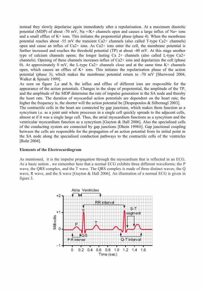
As mentioned, it is the impulse propagation through the myocardium that is reflected in an ECG. As a basic notion , we remember here that a normal ECG exhibits three different waveforms; the P wave, the QRS complex, and the T wave. The QRS complex is made of three distinct waves; the Q wave, R wave, and the S wave [Guyton & Hall 2006]. An illustration of a normal ECG is given in figure 3.

Immediately after the SA node has generated an impulse, the depolarisation of both atria occurs. This is reflected as the P wave in the ECG. The isoelectric line between the P wave and the Q wave corresponds to the conduction of the impulse through the AV node.The Q wave represents the depolarisation of the septum. The left part of the septum is depolarised before the right side, this causes the negativity of the Q wave. The R wave is caused by the propagation of the depolarisation wave in the septum towards the apex and afterwards depolarisation of the apex to the base of the heart. The S wave reflects the depolarisation of the posterior portion of the base of the left ventricle. Altogether, the Q, R, and S waves constitute the QRS complex, which represents the depolarisation of the ventricles [Martini 2004, Guyton&Hall 2006].. The QRS complex is a relative strong electrical signal because the ventricular muscle is much more massive than the atrial muscle [Guyton & Hall 2006, Martini 2004].The atrial repolarisation wave also called Ta is directly opposite in polarity to the P wave [Fuster et al. 2004]. The isoelectric line between the QRS complex and the T wave is the period where the entire ventricular myocardium is depolarised and repolarisation of the ventricles has not yet begun [Guyton & Hall 2006, Martini 2004].The T wave is the last wave appearing in a normal ECG and represents the repolarisation of the ventricular muscle.The positivity of the T wave is due to the propagation of the repolarisation wave, which spreads in reversed direction of the depolarisation wave [Martini 2004, Guyton & Hall 2006].

The appearance of the ECG is determined by the transmission of impulses through the heart, because, any changes in the trasmission pattern and velocity will affect the current flow around the heart and consequently affect the shape of the waves in the ECG. This can be understood by considering a vectorcardiographic representation of a depolarising muscle. During the propagation of the depolarisation wave a part of the muscle will be depolarised while the remaining part is still polarised. This causes a voltage difference between the two parts. The voltage difference is determined by the amount of depolarised and polarised muscle respectively; the largest difference is seen when half of the muscle mass is depolarised and the other half is not. The direction and magnitude of the current generated in the heart at a given instant can be depicted as a vector that points in the direction of the current flow and with length proportional to the voltage difference between depolarised and polarised muscle [Guyton& Hall 2006]. A representation of the magnitude and direction of the instantaneous mean electrical vector of the ventricles during the depolarisation is shown in figure 4.

Figure 4: Vectorcardiographic representation during the depolarisation of the ventricular muscle mass. I, II, and III corresponds to Einthoven’s bipolar leads. Edited from Guyton and Hall [2006].

By projecting the mean electrical vector onto the three bipolar leads (i.e. I, II, and III) a picture of the electrical activity measured by each lead is obtained [Sand et al. 2004, Guyton & Hall 2006]. The first step in figure 4 shows a short mean electrical vector because only small portion of septum is depolarised, thus all electrocardiographic voltages are low in the three bipolar leads. Next, the mean electrical vector is long because much of the ventricular muscle is depolarised, this is also shown as the shaded areas in figure 4. The voltage at lead II is greater comparing to the rest of the leads because the mean electrical vector extends almost in the same direction as the axis of lead II. Next, the depolarisation wave reaches the epicardium and the apex of the heart, the mean electrical vector becomes shorter and the electrocardiographic voltages becomes lower. The direction of the mean electrical vector is changing slowly toward the left side, due to the greater amount of ventricular muscle mass in the left side, thus slower depolarisation.Afterwards, the mean vector becomes shorter because only small portion of the ventricular muscle is still polarised.Furthermore the direction of the vector is toward the base of the left ventricle. In this case only lead I has positive electrical voltage.Finally, the entire ventricular muscle is depolarised and no current flows around the heart. Therefore, the mean electrical vector becomes zero and consequently the voltages measured in all leads become zero, as shown in figure 4.From the above, it can be seen that the ECG is determined by the pattern, amplitude, and velocity of the impulse propagation during cardiac activity. The ANS effects on these variables is therefore crucial to clarify whether the ANS has an effect on the morphology of the ECG or not.

Autonomic Innervation and Regulation of the Heart

The autonomic innervation of the heart is rich. Parasympathetic innervation is particularly rich to the SA node, sinoatrial conducting pathways, and the AV node, whereas the parasympathetic innervations to the ventricles are sparse [Wei-Jin et al. 2005, Malik 1998, Brodde & Michel 1999, Guyton & Hall 2006]. The sympathetic nervous system innervates all parts of the heart but is dominating in the ventricles [Wei-Jin et al. 2005, Guyton & Hall 2006].Figure 6 illustrates the sympathetic and parasympathetic innervations of the heart.

Figure 5: The sympathetic and parasympathetic innervation of the heart.

The parasympathetic innervation is dominating in the SA node, atrial myocardium, and the AV node compared to the ventricles. In contrast, sympathetic innervation dominates in the ventricles. (Guyton and Hall [2006])The two divisions have opposite effects on the heart; the sympathetic division causes excitation, whereas the parasympathetic causes inhibition. The parasympathetic division predominates in resting conditions whereas the sympathetic division dominates in more demanding situations [Martini 2004].

Parasympathetic Effects on Cardiac Cells

The parasympathetic nervous system releases acetylcholin at the postganglionic nerve endings. Acetylcholin binds to one or more subtypes of muscarinic (M) receptors in the human heart. Five different muscarinic receptor subtypes (M1-M5) have been identified. M2 is the predominating muscarinic receptor type in the heart [Brodde& Michel 1999]. An inhibitory G protein (Gi) is attached to the M2 receptor on the membrane of the cell. When acetylcholine binds to the M2 receptor, the Gi protein is activated, which causes an inhibition of adenylate cyclase. The inhibition of adenylate cyclase inhibits the formation of cyclic adenosine monophosphate (cAMP) from adenosine triphosphate (ATP) [Guyton & Hall 2006, Despopoulos & Silbernagl 2003]. cAMP would have activated type A protein kinase (PKA) which is capable of phosphorylating proteins. The absence of PKA causes a reduction of Ca 2+ influx, due to inactivation of L-type Ca2+ channels. Furthermore, the activation of the Gi protein opens potassium channels which causes an efflux of K+ from the cell leading to hyperpolarisation [Brodde & Michel 1999].

Sympathetic Effects on Cardiac Cells

The sympathetic nervous system uses epinephrine and norepinephrine as primary transmitter substances. There are two adrenergic receptor types.. When epinephrine or norepinephrinebinds to the adrenoceptor it activates a G protein in a manner similar to that of acetylcholine binding to M2 receptors.Instead of activating an inhibitory G protein, adrenoceptors activates a stimulatory G (Gs) protein. The activation of the Gs protein activates cAMP which in turn activates PKA [Sherwood 2004]. PKA phosphorylates Ltype Ca2+ channels which activates them, and consequently increases the

intracellular Ca2+ concentration [Kamp & Hell 2000]. This causes a positive chronotropic effect on the SA node and positive dromotropic effect on the AV node.

Autonomic Innervation and Regulation of the Heart

The increased concentration of cytosolic Ca2+ activates ryanodine receptors (RyR) in the sarcoplasmatic reticulum (SR). This causes a release of a large amount of Ca2+ from the SR to the cytosol. In the membrane of the SR, there is a Ca2+ pump called sarcoplasmatic reticulum Ca2+-ATPase (SERCA2), which pumps the cytosolic Ca2+ back into the SR. In humans, the activity of SERCA determines the rate of removal of more than 80% of cytosolic Ca 2+ [Frank et al. 2003]. SERCA2 pumps are regulated by a protein called phospholamban (PLB). Normally, PLB inhibits SERCA2, but under adrenergic stimulation PKA phosphorylates PLB and thereby reduces the inhibitory effect of PLB on SERCA2. This causes an increase of the rate of intracellular Ca2+ removal from the cytosol into the SR.The result of the described process is a rapid increase in intracellular Ca2+ concentration due to the RyR receptor but of short duration due to the Ca2+ removal mediated by SERCA2 [Fuster et al. 2004, Bers 2002]. This produces positive inotropic effects on the myocardium. The high concentration of the intracellular Ca 2+ increase the amplitude and decrease the duration of the action potential of the cardiac contractile cells [Parilak et al. 2009].

From the above discussion , it becames obvious that the ANS has great influence on the cardiac activity. In general, the parasympathetic division causes negative chronotropic, dromotropic, and inotropic effects to occur. In contrast, the sympathetic division causes positive chronotropic, dromotropic, and inotropic effects to occur. The intermingled picture presented, where systemic effects go hand-in-hand with cellular level features need to be supplemented by another very important element: the ANS also regulates the conductance of the gap junctions which connect adjacent cells in the heart. This implies a direct involvement of ANS in the structure of the conduction tissue that has very important consequences on its conductive properties and thus on the general ECG shape.

As mentioned before, gap junctions are responsible for the impulse propagation in the heart [Rohr 2004]. Gap junctions are regulated by different substances, among these are cAMP, PKA, and Ca 2+ [Dhein 1998b]. The concentration of these substances changes in the intracellular environment due to autonomic innervation. An increase in intracellular cAMP leads to increased coupling between adjacent cells [Dhein 1998b]. PKA enhances the conductance of the most abundant type of gap junction found in the heart. The change is very rapid and may last for several minutes. A large increase in intracellular Ca2+ causes reduction in conductance of the gap junctions.Under normal conditions the Ca2+ concentration does not reach sufficient levels to cause a reduction in gap junctional conductivity [Dhein 1998a].If the changes, in the mentioned substances mediated by the autonomic nervous system are high enough to cause a regulation of the cardiac gap junctions then, sympathetic innervation would cause an increase in gap junctional conductance, whereas the parasympathetic innervation would cause a decrease in gap junctional conductance. Going back to the initial problem of the effect of ANS on ECG shape and consequently on the HRV in terms of systemic variations of RR intervals) we can state that changes in the ECG are mediated by changes in the pattern of impulse propagation, the velocity of impulse propagation through the heart, and the amplitude of the voltage differences generated by the impulse.This allows us to make the subsequent general statements:

1) There has been a lot of confusion regarding the meaning of the different measures, especially in the frequency domain. In the early studies the spectral components were regarded as a reflection of the autonomic tone [Notarius ,Floras 2001], i.e the balance between the activity in the sympathetic and parasympathetic division [Martini 2004], but studies comparing the firing rates of vagal and sympthetic cardiac fibres with the sino-atrial response shows that the heart rate variations not necessarily correspond to variations in the mean firing rate, but also rather to the sino-atrial responsiveness to the changes in the autonomic tone [Notarius & Floras 2001].

2) ANS has great influence on the cardiac activity. In general, the parasympathetic division causes negative chronotropic, dromotropic, and inotropic effects to occur. In contrast, the sympathetic division causes positive effects to occur.

Interestingly, the analysis showed that sympathetic stimulation of the heart causes an increase in heart rate, an increase in conduction velocity through the AV node and myocardium, and an increased amplitude of the action potentials of cardiac contractile cells. The parasympathetic division inhibits the processes which causes these changes, thus, the parasympathetic division has the opposite effect. This encourages to believe that the morphology of the QRS complex changes with variation in ANS balance.Following such long and detailed discussion we have to pose a specific question.Have we to day a marker of the ANS activity that may be considered really suitable to take in accurate consideration the complex mechanisms that we have so far taken into consideration?

The Methodology of Analysis

We may now pass to introduce our methodology.The emerging indication from the previous studies is that we are in presence of a very complex system regulated from linear and non linear interrelationships and couplings. The most important feature is that such system exhibits an ANS balance that we must attempt to correctly evaluate.The answer to our previous posed question is that we need to introduce a new methodological treatment that is able to account for chronotropic, dromotropic, and inotropic effects to occur.

The use of spectral analysis implies that the event series can be represented by a sum of sinusoidal components, of different amplitude, frequency and phase values. Well defined fluctuations can be identified in distinct frequency bands, which have been attributed to the influence of vagal and/or sympathetic outflows. Various spectral methods for the calculation of power spectra density have been applied since the 1960's; they may be generally classified as non-parametric and parametric. The non-parametric approach mainly used is the Fast Fourier Transform (FFT) just to avoid statistical uncertainty related to the choice of the model order, which is inherent to the parametric PSD estimates.Traditional spectral analysis of heart rate variability (HRV) and blood pressure variability (BPV) results in a spectrum with three major components, defined as very low-frequency (VLF: 0.003 – 0.04 Hz), low-frequency (LF: 0.04 – 0.15 Hz) and highfrequency (HF: 0.15 – 0.4 Hz) .

Note the essential feature of the method. We speak here only of power.

The distribution of the power and the central frequency of these components are not fixed but vary in relation to changes in autonomic modulation of heart rate and blood pressure . Note some further limitations of the method. It is important to observe that a large proportion of the VLF component is due to nonharmonic noise (direct current - DC), rendering VLF assessment from short-term recordings a very dubious measure that should be avoided. Nevertheless this is the by-far most important power spectrum component, so reaching the conundrum that the most relevant

component in terms of explained variability of the HRV is in the same time the less rliable as for their quantitative estimation for the simple fact, at least in the short-term recordings setting it cannot be considered as being an oscillatory component at all. The LF and HF components are evaluated in terms of frequency (Hz) and power. This power is assessed by the area of each component and, therefore, squared units are used for its absolute value. In addition, an appraisal of the fractional distribution of power, independent of the absolute values of variance, can be obtained with computation of normalized units (nu). They are obtained by dividing the power of a given component by the total power from which the VLF has been subtracted. This procedure focuses on the possible reciprocal link between LF and HF components but remains somewhat controversial. In the framework of a correct methodological approach it remains thus to introduce a correct marker of ANS. In our opinion we may reach this objective starting from the conclusion that was reached from Zbiliut, Giuliani, i.e. that the main dynamical feature of hearbeat dynamics can be explained by a quantum-like model in which the system undergoes a jumping between adjacent states (adjacent in terms of RR length classes) in response to changes in the internal state (Giuliani A., G.Piccirillo, V.Marigliano, A.Colosimo (1998) A Non-linear Explanation for Aging Induced Changes in Heartbeat Dynamics. Am.Journ. Physiol. (Heart.Circ.Physiol. 275): H1455-H1461, . Giuliani A., P. Lo Giudice, A.M. Mancini, G. Quatrini, L. Pacifici, C.L. Webber, M. Zak and J.P. Zbilut (1996) A Markovian Formalization of Heart Rate Dynamics Evinces a Quantum-Like Hypothesis. Biological Cybernetics (74): 181-187). This ‘ jumps’ point to an intrinsically discrete kind of dynamics that happens at all the time scales (the fractal, scale invariant, nature of these state changes is descrive in Giuliani et al. (1996)] so asking for a less demanding (in terms of continuity and stationarity constraints) technique as Fourier Transform for adopting a frankly discrete and model independent analysis method.Linked to such conclusion is the notion of Recurrence that Zbilut and Webber were able to quantify by the well known methodology called RQA , Recurrence Quantification Analysis. Recurrence and Variability are two tightly related concepts. It is important to stress the functional meaning of the concept of variability in the realm of ANS regulation of HRV. At odds with the great majority of man-made tools in which the increase in variability is the signature of malfunctioning, in the case of heartbeat regulation the situation (at least when variability is confined ina given physiological range) is just the opposite: given HRV is the image in light of the fine-tuning of blood flux to the ever changing needs of the internal ‘milieu’ (as Claude Barnard defined the whole organism state) with the resulting heartbeat length as a sort of ‘majority vote’ or ‘integration’ of the various signals impinging on the heart from ANS, an high variability in time corresponds to an efficient sensing of the environment by the autonomic nervous system, while a low variability goes hand-in-hand with a less efficient control (as in the extreme case of heat transplanted patients where ANS control is practically abolished and the HRV is severely decreased). This is the main biological reason for focusing on the concept of Variability for the phenomenological estimation of chronotropic, dromotropic, and inotropic effects.Let us explain the matter in more detail. Let us observe that we are in presence of non linear processes. They are the anteroom of arising very complex dynamicis crossing of the frontier of the chaotic processes. From the conceptual point of view thare is only one variable that is able to account for such complex biological behaviours and it is that one of Recurrence. It was introduced by Eckmann and subsequently developed by Zbilut and Webber in the well established methodology of analysis that is actually provided with reference as RQA ( Recurrence Quantification Analysis) [ C.L. Webber, J.P. Zbbilut,1994 ]..While the basic idea of Recurrence is immediately intuitive ‘The periodic character of a series can be quantified by the number of times the same pattern (letter, number, symbol..) recurs in the series’ and this immediacy and freedom from mathematical assumptions makes RQA apt to model complex nonlinear systems, it is worth noting to go more in depth into the subtleties of the concept

of Recurrence. In doing so we will rely upon explanation that was furnished rather recently by Norbert Marwan, in his excellent paper entitled: Recurrence plots for the analysis of complex systems that he wrote with coauthors: Carmen Romano, Marco Thiel, and Jurgen Kurths and appeared on Physics Reports, 438 (2007) 237 – 329

We adopt here his introduction to this basic concept:

If we observe the sky on a hot and humid day in summer, we often “feel” that a thunderstorm is brewing. When children play, mothers often know instinctively when a situation is going to turn out dangerous. Each time we throw a stone, we can approximately predict where it is going to hit the ground. Elephants are able to find food and water during times of drought. These predictions are not based on the evaluation of long and complicated sets of mathematical equations, but rather on two facts which are crucial for our daily life:(1) similar situations often evolve in a similar way;(2) some situations occur over and over again.The first fact is linked to a certain determinism in many real world systems. Systems of very different kinds, from very large to very small time–space scales can be modelled by (deterministic) differential equations. On very large scales we might think of the motions of planets or even galaxies, on intermediate scales of a falling stone and on small scales of the firing of neurons. All of these systems can be described by the same mathematical tool of differential equationsThey behave deterministically in the sense that in principle we can predict the state of such a system to any precision and forever once the initial conditions are exactly known. Chaos theory has taught us that some systems—even though deterministic—are very sensitive to fluctuations and even the smallest perturbations of the initial conditions can make a precise prediction on long time scales impossible. Nevertheless, even for these chaotic systems short-term prediction is practicable.The second fact is fundamental to many systems and is probably one of the reasons why life has developed memory.Experience allows remembering similar situations, making predictions and, hence, helps to survive. But remembering similar situations, e.g., the hot and humid air in summer which might eventually lead to a thunderstorm, is only helpful if a system (such as the atmospheric system) returns or recurs to former states. Such a recurrence is a fundamental characteristic of many dynamical systems.They can indeed be used to study the properties of many systems, from astrophysics (where recurrences have actually been introduced) over engineering, electronics, financial markets, population dynamics, epidemics and medicine to brain dynamics. The methods described in this review are therefore of interest to scientists working in very different areas of research. The formal concept of recurrences was introduced by Henri Poincaré in his seminal work from 1890 [1], for which he won a prize sponsored by King Oscar II of Sweden and Norway on the occasion of his majesty’s 60th birthday. Therein, Poincaré did not only discover the “homoclinic tangle” which lies at the root of the chaotic behaviour of orbits, but he also introduced (as a by-product) the concept of recurrences in conservative systems. When speaking about the restricted three body problem he mentioned: “In this case, neglecting some exceptional trajectories, the occurrence of which is infinitely improbable, it can be shown, that the system recurs infinitely many times as close as one wishes to its initial state.” (translated from [1]) Even though much mathematical work was carried out in the following years, Poincaré’s pioneering work and his discovery of recurrence had to wait for more than 70 years for the development of fast and efficient computers to be exploited numerically. The use of powerful computers boosted chaos theory and allowed to study new and exciting systems. Some of the tedious computations needed

to use the concept of recurrence for more practical purposes could only be made with this digital tool.In 1987, Eckmann et al. introduced the method of recurrence plots (RP) to visualise the

recurrences of dynamical systems. Suppose we have a trajectory [ ]N

iix 1=

i=1 of a system in its

phase space [2]. The components of these vectors could be, e.g., the position and velocity of a pendulum or quantities such as temperature, air pressure, humidity and many others for the atmosphere. The development of the systems is then described by a series of these vectors, representing a trajectory in an abstract mathematical space. Then, the corresponding RP is based on the following recurrence matrix:

Ri,j = ji

ji

xxifxxif

≈≠

10

_where N is the number of considered states and ji xx ≈ means equality up to an error (or distance) ε. Note that this ε is essential as systems often do not recur exactly to a formerly visited state but just approximately. Roughly speaking, the matrix compares the states of a system at times i and j. If the states are similar, this is indicated by a one in the matrix, i.e. Ri,j =1. If on the other hand the states are rather different, the corresponding entry in the matrix is Ri,j =0. So the matrix tells us when similar states of the underlying system occur. In conclusion, if we consider a given time series, as example, a time series made by R-R intervals. Recurrence, as example for the point iRR − and 5+− iRR , means that we have iRR − -value ≈

5+− iRR - value in the limit of a prefixed convergence value ε.The concept of Varibility is in itself the exact conceptual counterpart of the concept of Recurrence. Given a time series of N intervals RR − , points realizing the greatest recurrence will give correspondgly the minimum variability. On the other hand, points giving the minimum recurrence will correspondgly exhibit maximum variability. When we speak of counterpart we do not intend Recurrence is NOT the simple ‘opposite’ of Variability, if this would be the case we obviously had no need of another parameter given we should simply use variability and look at it in the two directions of increase/decrease. The point is that Recurrence catches the ‘order dependent’ portion of variability while variability as such (i.e. standard deviation of RR intervals) is totally independent from order, i.r. from the actual dynamics of the studied series. Let’s imagine a series like this 1,2,3,1,2,3,1,2,3 (series A) and a series A’ : 3,2,1,2,2,1,3,3,1 they have the same standard deviation (SD=1), buth while the first is shows an highly recurrent behavior in time the second is totally random. If we measure the recurrence of A by taking an embedding dimension of three (i.e. considering atomic elements made up of three consecutive values we obtain a Recurrence = 100%, while the second does not show any Recurrence). This different consideration of what Variability (and thus the nature of ANS control exerted on heart) is, allows us to discover periodic endogenous ‘cycles’ in which the system get entrapped (and thus implying a decoupling from the continuous adaptation to a stochastic environment) nor simple variability, nor FFT can put into light.

This is the essence of the CZF method that is based on Recurrence Quantification.The details of the method have been exposed by us elsewhere (see as example the section devoted to selected publications in this site) but we may mention here again some essential feature.Let us take as reference a given time series of N , RR − intervals.In the current analysis of HRV we just use a concept of ‘order dependent’ variability that, in the case of Poincaré plot is only limited to adjacent beats .In fact, by using such technique we plot ( )1 ii RRRR −−− + and thus just we estimate the correlation between two adjacent points. In our case we need a more far reaching method encompassing different periods variability . In particular, we need to estimate, as ANS marker, the variability for each pair of RR − points, the first time considering adjacent points, the next time considering variability between iRR − and 2+− iRR , the third time between iRR − and 3+− iRR

, and, in general, between iRR − and τ+− iRR . Calling τ the lag , and varying at each step the Lag τ from 1 to ( )3−N , we will estimate the variability for each pair of points in the given

RR − time series, and covering this time the exploration of the whole series for any possible time interval. Take the Lag 1=τ , we will estimate the total variability induced from the ANS for all the adjacent points of the given series of intervals. Take the Lag 2=τ , we will estimate this time the total variability , induced from the ANS, for all the point shifted by one. Take the Lag 3=τ , we will estimate the total variability induced from the ANS between points shifted by 3 and so on. In this manner we reconstruct the variability that is induced from ANS starting from adjacent RR −values and advancing , step by step, each time of a shift given by one Lag. We characterize in this manner the variability as new marker of the ANS on the given recorded RR − time series.

We may now mention the particular algorithm that we use for the calculation of the order-dependent variability. It is called the Variogram. We do not repeat here the formulas just to unburden the tratment from mathematical formulas but the details of the mathematical treatment have been given by us elsewhere. Finally, we arrive to estimate the final variogram and a plot in which in abscissa we have the values of the Lags that we have considered, and in ordinate we have the value of the new ANS marker, that is to say , the values of the calculated total variability in correspondence of each Lag.The next and final step is now easy to reach. We may pass from the domain of the time (the Lags) to the domain of the Frequency by a proper transformation so that we have finally the values of the total variability this time corresponding to the given frequency. This is quite similat to what is realized by FFT. In abscissa we have the values of the frequencies. In ordiante, this time we have the true values of the variability and not the PSD. Also in the case of the CZF method we will consider, as in FFT, three basic frequency bands, the VLF, the LF, and the HF and for each band we will have the value of the total variability. In this manner we will proceed to calculate standard indeces as LF/HF (balance) (it will indicate in this case the ratio between the total variability in the LF and HF bands), we still will calculate the VLF%, the LF%, the HF%, the VLF, LF, and HF in n.u. and still the value of the ratios VLF/LF+HF or LF/(LF+HF) or HF/(LF+HF)). In conclusion, the visual inspection will give results as in the FFT case with the basic differnce that in the case of the FFT we are expressing the power of the modulation . In the case of the CZF method we are estimating instead the variability. We will have also new quantitative markers that obviously will account this time for chronotropic, dromotropic, and inotropic effects to occur.

The Limitations of the FFT.We had various posibilities to outline some insufficiences in application of FFT in ananlysis of R-R intervals. We would add here still some further comments.

We first remind ourselves of three basic properties of the FFT (Fast Fourier Transform) process.

Generally speaking:

• First, information in signal must be preserved during transformation. That is, the variable measured on time signal must equal the variable measured on the frequency representation of that signal.

• Second, an FFT converts the signal representation between time and frequency domains. The time domain representation shows when something happens and the frequency domain representation shows how often something happens.

• Finally, an FFT assumes that the signal is repetitive and continuous. Other strong requirements are discuseed by us elsewhere [ see the section selected publications of this site]

Let us take a standard example as well discussed and available on line (New Version of DATS software, http://blog.prosig.com/2009/07/20/data-windows-what-why-and-when/).

Let us take the case of a 10 Hz sinusoid (Figure 6). This signal is periodic within the time record used to calculate the spectrum.

Figure 6: the 10 Hz sinusoidal time series

If we perform an FFT, the result, shown below, will consist of a single line in the spectrum with an amplitude that represents, as example, the rms in relation to the time series amplitude.

Figure 6: FFT of 10Hz sinusoid

Now, let us consider a second example. In this case (Figure 7) we have a 9.5 Hz sinusoid.

Figure 7: 9.5 Hz Sinusoid

If we perform an FFT operation on this signal, it yields the multi-line spectrum shown in Figure 8.

Figure 8: Multi-line spectrum (FFT of 9.5 Hz sinusoid)

The important thing to consider is that we no more obtain a single line spectrum. It is still a sinusoid but its spectrum is a multi-line spectrum as erroneously seen by the FFT process. It assumes the signal to be periodic (not only within a single record) and on-going or continuous. The 9.5 Hz signal (Figure 7), seen in analog form, is on-going and continuous, but when viewing it from a digital perspective (discrete number of samples in a specified time block), this signal is not a sinusoid (see Figure 9).

Figure 9: 9.5 Hz sinusoid (End-to-end)

This is the reason because the FFT produces the multi-line spectrum in figure 4 with no less than 20 visible lines. A totally deformed result.

At this point, in R-R FFT analysis a problem becomes of crucial importance.

How may we minimize the effects of such discontinuities? Note that we speak about the methodological manner to minimize, not to cancel such undesidered effects. The possibility is that we use something called a “window”. Typically, the window used for most general purpose data is the “Hanning” or “Von Hann”.

The “Von Hann” or “Hanning” window is named after Julius Von Hann (1839-1921). Von Hann was an Austrian meteorologist and is seen as the father of modern meteorology. He was the director of the Central Institute for Meteorology in Vienna (1887-1897), professor of meteorology at the University of Graz (1897-1890) and professor of cosmic physics at the University of Vienna (1890-1910). In signal processing the Hann function was named after him by R. B. Blackman and John Tukey in “Particular Pairs of Windows.” published in “The Measurement of Power Spectra, From the Point of View of Communications Engineering”, New York: Dover, 1959, pp. 98-99.

Multiplying the window function (Figure 10) by the original time signal forces the signal to zero at the beginning and end of each time record (Figure 11). Placing multiple time records shown end to end shows the signal is now forced to be periodic when the time records are placed end to end. One problem solved, but the signal now in each of the time records is not a sinusoid any longer. This modification to the sinusoid is represented in the frequency domain by 4 dominant lines in the frequency representation of the signal plus also other

Figure 10: The "Hanning" window

Figure 11: Sinusoid multiplied by window

Figure 12: Spectrum of 9.5Hz sinusoid (after windowing)

The spectrum which was 20 lines before applying the Hanning Window function has now been reduced to a spectrum of only 4 lines plus other lines of reduced values but however present. The result is thus not extremely accurate , but reaches a much closer representation respect to the single line spectrum one would expect for the single frequency time signal. Obviously, one must remember here that, calculating HRV in VLF, LF, and HF bands, we integrate into some previously

prefixed bands of frequency and thus the presence in such bands of such , also if reduced, undesidered peaks, may alter totally the goodness of the estimated so called variabilities in PSD. In addition, let us see what happens to the single line spectrum from the 10 Hz single frequency time signal. Instead of a single line spectrum, the modified single frequency signal now is represented by a 3 line spectrum (Figure 13). There is no loss in amplitude read out accuracy, but a loss in frequency resolution is evident and particularly affecting negatively the estimations that we perform.

Figure 13: Spectrum of 10Hz sinusoid (after windowing)

We should have to discuss here what it happens about the data that are being missed at the beginning and end of each record. Data are being reduced and/or set to zero over one half the time record. To assume events happening in the region of reduced amplitude areas, a processing technique exists called “overlap” processing. By applying this technique, the events occurring at or near the beginning and ending of the time records are enhanced by using overlap processing. Figure 14 represents records being processed “end-to-end” or 0% overlap. Figure 15 shows overlap of 50%.

Figure 14: End-to-end (0% overlap)

Figure 15: 50% overlap

Typically 67% overlap (Figure 16) is considered sufficient to weight the events near the beginning/end of the time record, however 75% overlap (Figure 17) is somewhat better. Today, with the high processing capabilities of computers, there is little reason not to utilize overlap processing.

Figure 16: 67% overlap

Figure 17: 75% overlap

Different shapes of the windowing function dictate what the spectrum shaping looks like. The table below lists a few window function types. All Window functions that operate on the time domain signals typically zero out the beginning and end of time record. The obvious exceptions to this are the “force” and “exponential decay” windows used in hammer/modal applications.

Type When to useRectangular Only when signal is known to be periodic within time recordHanning Most often used for general purposeFlat top When absolute amplitude accuracy is required – calibration/sensitivity checkKaiser-Bessel When relatively high amplitude accuracy and frequency resolution are important

Results.In order to evaluate the possibilities of the FFT as marker of ANS, we studied a number of normal subjects using a sampling frequency of 250 Hz in ECG recording and thus selecteing each time a piece of R-R intervals and comparing obviously each time HRV calculated on the same epoc lengths.The aim was to compare the results that may be obtained using some different windows.Let us inspect the results for the different normal subjects that we examined.