On Cox processes and credit risky securities1

David Lando

Department of Operations Research

University of Copenhagen

Universitetsparken 5

DK-2100 Copenhagen �.

Denmark

phone: +45 35 32 06 83

fax: +45 35 32 06 78

e-mail: dlando@math.ku.dk

First version: March 1994

This revision March 31, 1998

1Previous title: On Cox processes and credit risky bonds. This paper is a

revised and extended version of parts of Chapter 3 of my Ph.D. thesis. I have

received useful comments from my committee members Robert Jarrow, Rick Dur-

rett, Sid Resnick and Marty Wells, as well as from Michael Hauch, Brian Huge,

Martin Jacobsen, Monique Jeanblanc, Kristian Miltersen, Lasse Heje Pedersen,

Torben Sk�deberg and Stuart Turnbull and from participants at seminars at the

1993 FMA Doctoral seminar in Toronto, Merrill Lynch, Aarhus University, Odense

University, University of Copenhagen, Stockholm School of Economics, University

of Lund, New York University, Erasmus University, the 1994 Risk conference in

Frankfurt, IBC conference on Credit derivatives in London 1996, the 1996 confer-

ence on Mathematical Finance in Aarhus. All errors are of course my own.

1 Introduction

The aim of this paper is to illustrate how Cox processes - also known as doubly

stochastic Poisson processes - provide a useful framework for modeling prices

of �nancial instruments in which credit risk is a signi�cant factor. Both the

case where credit risk enters because of the risk of counterparty default and

the case where some measure of credit risk such as a credit spread is used as

an underlying variable in a derivative contract can be analyzed within our

framework.

The key contribution of the approach is the simplicity by which it allows

credit risk modeling when there is dependence between the default-free term

structure and the default characteristics of �rms. As an illustration of the

method we present a generalized version of a Markovian model presented in

Jarrow, Lando and Turnbull [13]. This generalization allows the intensities

which control the default intensities and the transitions between ratings todepend on state variables which simultaneously govern the evolution of theterm structure and possibly other economic variables of interest. This model

can be used to analyze a variety of contracts in which credit ratings anddefault are part of the contractual setup. Two important examples are de-fault protection contracts which provide insurance against default of a �rm

and so-called 'credit triggers' in swap contracts which typically demand thesettlement of a contract in the event of downgrading of one of the parties

to the contract. By imposing some additional structure on the model wederive a new class of models which in a special setup become 'sums of a�neterm structure models'. These models simultaneously model term structures

for di�erent ratings and allow spreads to uctuate randomly even in peri-ods where the rating of the defaultable �rm does not change. Such models

are useful for managers of corporate bond portfolios (and risky governmentdebt) who are constrained by credit lines setting upper limits on the amountof bonds held below a certain rating category. Given such lines the event of

a downgrading may force the manager to either sell o� part of the positionor try to o�-load some credit exposure in credit derivatives markets.

The modeling framework is similar to that of Jarrow and Turnbull [14],

Jarrow, Lando and Turnbull [13], Lando [16], Madan and Unal [19], Artzner

and Delbaen [1], Du�e and Singleton [7], [8], and Du�e, Schroder and Ski-

adas [9] in that default is modeled through a random intensity of the defaulttime. However, this paper dispenses with the independence assumption em-ployed in Jarrow and Turnbull [14], Jarrow, Lando and Turnbull [13], Madan

1

and Unal [19]. In this respect our approach resembles that of the works of

Du�e and Singleton [7],[8], and Du�e, Schroder and Skiadas [9]. The ap-

proach in this paper is not based on the recursive methods employed there.

This sacri�ces some generality but the structure of Cox processes produces

a class of models which are simple to derive yet seems rich enough to handle

important applications when only one-sided credit risk is considered. For an

analysis of two sided default risk in an intensity-based framework, see Du�e

and Huang [6].

The pros and cons of modeling default in an intensity-based framework as

opposed to using the classical approach originating in Black and Scholes [2]

and Merton [20] are discussed elsewhere, see for example Du�e and Single-

ton [7],[8], and the review papers by Cooper and Martin [3] and Lando [17].

Here we simply note that this paper and the work by Du�e and Singleton [8]

point to one important advantage of the intensity-based framework, namelythe fact that the intensity based framework is capable of reducing the tech-

nical di�culties of modeling defaultable claims to the same one faced whenmodeling the term structure of non-defaultable bonds and related derivatives.

The structure of the paper is as follows: In section 2 we outline the basic

construction of a Cox process, concentrating on the �rst jump time of such aprocess. Knowing how to construct a process means knowing how to simulate

it. Hence this section is important if one wants to implement the models.Furthermore, the explicit construction gives the key to proving the resultslater on by - essentially - using properties of conditional expectations.

Section 3 then shows how to calculate prices of three 'building blocks' fromwhich credit risky bonds and derivatives can be constructed. Several exam-ples of claims are given which are constructed from these building blocks.

Within this framework we have great exibility in how we specify the be-havior of the state variables which simultaneously determine the default free

term structure and the likelihood of default. When di�usions are used asstate variables, the Feynman-Kac framework handles pricing of credit risky

derivative securities in virtually the same way as it handles derivatives in

which credit risk is not present. That particular setup is one of 'di�usionwith killing' - a special case of the general framework. We also outline how

the notion of fractional recovery, as introduced in Du�e and Singleton [8],

may be viewed in terms of thinning of a point process.Section 4 is an applications of the methodology. It is shown how a Marko-

vian model proposed by Jarrow, Lando and Turnbull [13] may be generalizedto include transition rates between credit ratings which depend on the state

2

variables. One important aspect of this generalization is that credit spreads

are allowed to uctuate randomly even between ratings transitions. Section

5 gives a concrete implementation of the generalized Markovian model by

considering an a�ne model for both the interest rate and the transition in-

tensities. It is shown how one can calibrate the model across all credit classes

simultaneously to �t initial spot rate spreads and the sensitivities of these

spreads to changes in the short treasury rate. Section 6 concludes.

2 Construction of a Cox process

Before setting up our model of credit risky bonds and derivatives, we give

both an intuitive and a formal description of how the default process is

modeled. The formal description is extremely useful when performing cal-culations and simulations of the model, whereas the intuitive description is

helpful when the economic content of the models are to be understood.Recall that an inhomogeneous Poisson process N with (non-negative)

intensity function l(�) satis�es

P (Nt �Ns = k) =

�Rt

sl(u)du

�k

k!exp

��Z

t

s

l(u)du

�k = 0; 1; : : : :

In particular, assuming N0 = 0; we have

P (Nt = 0) = exp

��Z

t

0l(u)du

�:

A way of simulating the �rst jump � of N is to let E1 be a unit exponentialrandom variable and de�ne

� = infft :Z

t

0l(u)du � E1g (2.1)

A Cox process is a generalization of the Poisson process in which the

intensity is allowed to be random but in such a way that if we condition on

a particular realization l(�; !) of the intensity, the jump process becomes aninhomogeneous Poisson process with intensity l(s; !):

In this paper we will write the random intensity on the form

l(s; !) = �(Xs)

3

where X is an Rd�valued stochastic process and � : Rd ! [0;1) is a non-

negative, continuous function. The assumption that the intensity is a func-

tion of the current level of the state variables, and not the whole history, is

convenient in applications, but it is not necessary from a mathematical point

of view.

The state variables will include interest rates on riskless debt and may

include time, stock prices, credit ratings and other variables deemed relevant

for predicting the likelihood of default. Intuitively, given that a �rm has

survived up to time t; and given the history of X up to time t; the probability

of defaulting within the next small time interval �t is equal to �(Xt)�t +

o(�t):

Formally, we have a probability space (;F ; P ) large enough to support

an Rd�valued stochastic process X = fXt : 0 � t � Tfg which is right-

continuous with left limits and a unit exponential random variable E1 whichis independent of X: Given also is a function � : Rd ! R which we assume

is non-negative and continuous. From these two ingredients we de�ne thedefault time � as follows:

� = infft :Z

t

0�(Xs)ds � E1g: (2.2)

This default time can be thought of as the �rst jump time of a Cox processwith intensity process �(Xs): Note that this is an exact analogue to equation

(2:1) with a random intensity replacing the deterministic intensity function.When �(Xs) is large, the integrated hazard grows faster and reaches the

level of the independent exponential variable faster, and therefore the prob-

ability that � is small becomes higher. Sample paths for which the integralof the intensity is in�nite over the interval [0; Tf ] are paths for which default

always occurs.From the de�nition we get the following key relationships:

P (� > tj (Xs)0�s�t

�= exp

��Z

t

0

� (Xs) ds

�t 2 [0; Tf ] (2.3)

P (� > t) = E exp

��Z

t

0� (Xs) ds

�t 2 [0; Tf ] (2.4)

What we have modeled above, is only the �rst jump of a Cox process.When modeling a Cox process past the �rst jump - something we will need in

Section 4 - one has to insure that the integrated intensity stays �nite on �nite

intervals if explosions are to be avoided. One then proceeds as follows: Given

4

a probability space (;F ; P ) large enough to support a standard unit rate

Poisson process N with N0 = 0 and a non-negative stochastic process �(t)

which is independent of N and assumed to be right-continuous and integrable

on �nite intervals, i.e.

�(t) :=Z

t

0

�(s)ds <1 t 2 [0; T ]

Then �(0) = 0 and � has non-decreasing realizations. Now de�ning

~Nt := N (� (t))

we have a Cox process with intensity measure �: For the technical conditions

we need to check to see that this de�nition makes sense, see Grandell [12] pp.

9-16. This approach is also relevant when extending the models presented inthis paper to cases of repeated defaults by the same �rm.

3 Three basic building blocks

The model for the default-free term structure of interest rates is given by

a spot rate process, a money market account and an equivalent martingalemeasure to which all expectations in this paper refer:

B(t) = exp

�Zt

0

rsds

�p(t; T ) = E

B(t)

B(T )

�����Ft

!

The default time � is modeled using the framework described in the pre-

vious section. The intensity process is denoted �:Hence we may write the

information at time t as

Ft = Gt _ Ht

where processes relevant in determining values of the spot rate and the hazardrate of default are adapted to G and

Ht = �f1f��sg : 0 � s � tg

5

holds the information of whether there has been a default at time t: Most

applications will be built around a state variable process X, in which case

we write R(Xt) for the spot rate rt at time t and the informational setup may

be stated as

Gt = �fXs : 0 � s � tg

Ht = �f1f��sg : 0 � s � tg

Ft = Gt _ Ht

Ft then corresponds to knowing the evolution of the state variables up to

time t and whether default has occurred or not.

Apart from the default characteristics and the default-free term structure

of interest rates what we need to know to price a defaultable contingent claim

are its promised payments and its payment in the event of default (i.e. itsrecovery). The basic building blocks in constructing such claims are

1. X1f�>Tg: A payment X 2 GT at a �xed date which occurs if there has

been no default before time T . As an example think of a vulnerableEuropean option, i.e. an option whose issuer may default before theoption's expiration. A possible partial recovery can be captured in

two ways: Let �T be a GT�measurable random variable, and think ofpartial recovery either as a recovery at the time of maturity of the form�T1f��Tg = �T��T1f�>Tg;which consists of a non-defaultable claim and

our �rst basic building block, or a recovery at the time of default as inthe third building block below.

2. Ys1f�>sg: A stream of payments at a rate speci�ed by the Gt�adaptedprocess Y which stops when default occurs. This may be used to model

idealized swaps in which we think of payments taking place continuallyin time. A possible recovery is captured by the next building block.

3. A recovery payment at the time of default of the form Z� where Z

is a Gt�adapted stochastic process and where Z� = Z�(!)(!): For a

contingent claim expiring at date T; think of Z as being 0 after time

T: This building block models a resettlement payment at the time of

default.

Note that the random variable X and the process Y can be thought of

as promised payments, whereas the payment captured by Z is an actual

payment at the time of default.

6

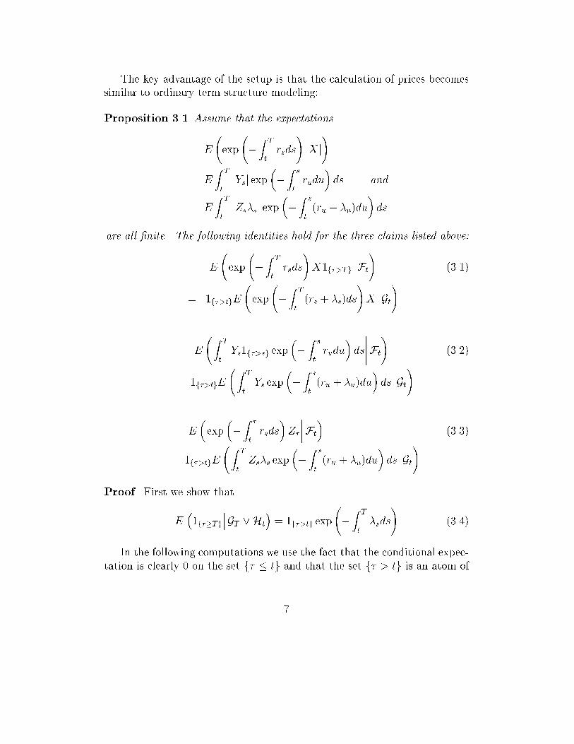
The key advantage of the setup is that the calculation of prices becomes

similar to ordinary term structure modeling:

Proposition 3.1 Assume that the expectations

E

exp

�Z

T

t

rsds

!jXj

!

E

ZT

t

jYsj exp��Z

s

t

rudu

�ds and

E

ZT

t

jZs�sj exp

��Z

s

t

(ru + �u)du

�ds

are all �nite. The following identities hold for the three claims listed above:

E

exp

�Z

T

t

rsds

!X1f�>Tg

�����Ft

!(3.1)

= 1f�>tgE

exp

�Z

T

t

(rs + �s)ds

!X

�����Gt!

E

ZT

t

Ys1f�>sg exp

��Z

s

t

rudu

�ds

�����Ft

!(3.2)

= 1f�>tgE

ZT

t

Ys exp

��Z

s

t

(ru + �u)du

�ds

�����Gt!

E

�exp

��Z

�

t

rsds

�Z�

����Ft

�(3.3)

= 1f�>tgE

ZT

t

Zs�s exp

��Z

s

t

(ru + �u)du

�ds

�����Gt!

Proof. First we show that

E�1f��Tg

���GT _Ht

�= 1f�>tg exp

�Z

T

t

�sds

!(3.4)

In the following computations we use the fact that the conditional expec-tation is clearly 0 on the set f� � tg and that the set f� > tg is an atom of

7

Ht: Therefore

E�1f��TgjGT _ Ht

�= 1f�>tgE

�1f��TgjGT _Ht

�= 1f�>tg

P (f� � Tg \ f� > tg jGT )

P (� > tjGT )

= 1f�>tgP (� � T jGT )

P (� > tjGT )

= 1f�>tgexp

��RT

0 �sds�

exp��Rt

0 �sds�

= 1f�>tg exp

�Z

T

t

�sds

!which proves (3.4).

Now consider (3.1).

E

exp

�Z

T

t

rsds

!X1f�>Tg

�����Ft

!

= E

E

exp

�Z

T

t

rsds

!X1f�>Tg

�����GT _ Ht

!jFt

!

= E

exp

�Z

T

t

rsds

!XE

�1f�>Tg

���GT _ Ht

������Ft

!

= 1f�>tgE

exp

�Z

T

t

rs + �sds

!X

�����Ft

!Now we want to replace the conditioning on Ft with conditioning on G.

Recall that E1 is a unit exponential random variable which is independent

of the sigma �eld GT : In particular, E1 is independent of the sigma �eld��exp

��RT

t(rs + �s) ds

�X�_ Gt and therefore (see Williams [21] 9.7(k))

E

exp

�Z

T

t

rs + �sds

!X

�����Gt _ �(E1)

!(3.5)

= E

exp

�Z

T

t

rs + �sds

!X

�����Gt!:

But we also have the following inclusion among sigma �elds:

Gt � Gt _Ht � Gt _ �(E1): (3.6)

8

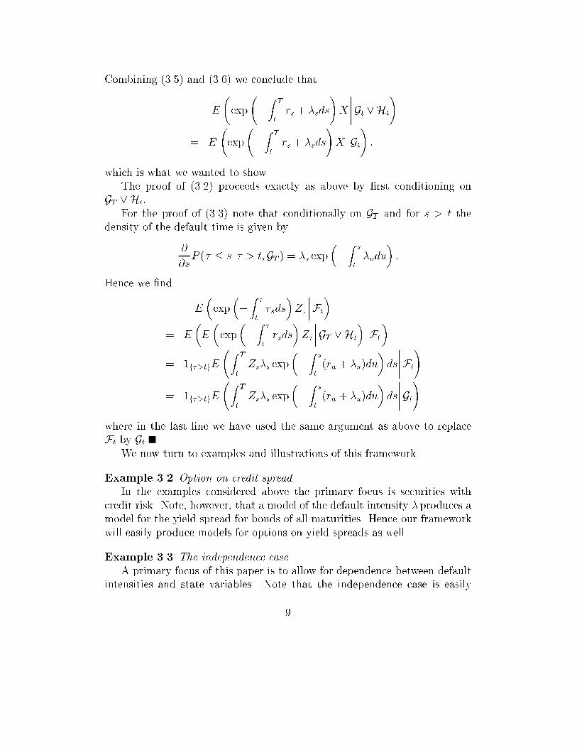
Combining (3.5) and (3.6) we conclude that

E

exp

�Z

T

t

rs + �sds

!X

�����Gt _Ht

!

= E

exp

�Z

T

t

rs + �sds

!X

�����Gt!:

which is what we wanted to show.

The proof of (3.2) proceeds exactly as above by �rst conditioning on

GT _ Ht:

For the proof of (3.3) note that conditionally on GT and for s > t the

density of the default time is given by

@

@sP (� � sj � > t;GT ) = �s exp

��Z

s

t

�udu

�:

Hence we �nd

E

�exp

��Z

�

t

rsds

�Z�

����Ft

�= E

�E

�exp

��Z

�

t

rsds

�Z�

����GT _Ht

�jFt

�= 1f�>tgE

ZT

t

Zs�s exp

��Z

s

t

(ru + �u)du

�ds

�����Ft

!

= 1f�>tgE

ZT

t

Zs�s exp

��Z

s

t

(ru + �u)du

�ds

�����Gt!

where in the last line we have used the same argument as above to replaceFt by Gt

We now turn to examples and illustrations of this framework.

Example 3.2 Option on credit spread.

In the examples considered above the primary focus is securities with

credit risk. Note, however, that a model of the default intensity � produces a

model for the yield spread for bonds of all maturities. Hence our framework

will easily produce models for options on yield spreads as well.

Example 3.3 The independence case.

A primary focus of this paper is to allow for dependence between default

intensities and state variables. Note that the independence case is easily

9

captured as well. In the state variable formulation we would simply let X =

(X1; X2) with X1 and X2 independent processes and de�ne the spot rate

as the process r(X1) and the default intensity process as �(X2): Of course,

either of these processes may be included as a state variable themselves.

Example 3.4 (Feynman-Kac representation).

An important special case is when

Gt = �fXs : 0 � s � tg (3.7)

where X is an Rd�valued di�usion process with di�usion matrix a(x; t) and

drift vector b(x; t) and in�nitesimal generator

AtF (x) :=1

2

dXi=1

dXk=1

aik(t; x)@2F (x)

@xi@xk+

dXi=1

bi(t; x)@F (x)

@xiF 2 C2(Rd)

Let T = Tf and let f : Rd ! R; g : [0; T ] � Rd ! R and k : [0; T ]� Rd ![0;1) be continuous functions. Note that when (3.7) holds, the relations(3.1),(3.2) and (3.3) are all of the form1

v(t; x) = Et;x

f (XT ) exp

�Z

T

t

k(u;Xu)du

!!

+Et;x

ZT

t

g(s;Xs) exp

��Z

s

t

k(u;Xu)du

�ds

!(3.8)

Hence, under suitable regularity conditions2 on the di�usion coe�cientsand on the functions f; g; k; the expectation in (3.8) is also a solution (satis-fying an exponential growth condition) to the Cauchy problem

�@v

@t+ kv = Atv + g [0; T ]�Rd

v(T; x) = f(x) x 2 Rd

and we see that the credit risky securities can be modeled using exactly the

same techniques as default-free securities.

1Note that in this section we will explicitly write time dependence of payments, spot

rates and hazard rates. In previous sections time dependence is possible simply by let-

ting one of the state variables be time - here we prefer to separate it from the di�usion

components.2See Karatzas and Shreve [15] and Du�e [5] for results and references to some of the

literature on which combinations of conditions one can impose to obtain this correspon-

dence.

10

Example 3.5 Fractional recovery and thinning.

In Du�e and Singleton [8], and Du�e, Schroder and Skiadas [9] a notion

of fractional recovery is considered which allows not only the intensity but the

recovery rate to enter into the expression for the default adjusted spot rate

process. Here we sketch how this may be given a simple interpretation in the

Cox process framework through the notion of thinning. Receiving a fraction

�tof pre-default value in the event of default of a contract is equivalent, from

a pricing perspective, to receiving the outcome of a lottery in which the full

pre-default value is received with probability (under the martingale measure)

�tand 0 is received with probability 1� �

t; i.e the event of default has been

retained with probability 1 � �t. This in turn may be viewed as a default

process in which there is 0 recovery but where the default intensity has been

thinned using the process �; producing a new default intensity of �(1� �):

In the case of a claim with promised payment XT and fractional recovery atthe default date of �

�one then obtains that with Z� = �

�c��; the price of

this claim at time t is given as

ct = E

exp

�Z

T

t

rsds

!X1f�>Tg + exp

��Z

�

t

rsds

�Z�1ft<��Tg

�����Ft

!

= 1f�>tgE

exp

�Z

T

t

(rs + �s(1� �s))ds

!X

�����Gt!:

4 A generalized Markovian model

In this section, as a concrete application of the framework presented above.we show how to generalize the model described in Jarrow, Lando and Turn-

bull [13] for pricing defaultable bonds. It is shown how the model can begeneralized to incorporate state dependence in transition rates and risk pre-

mia allowing for stochastic changes in credit spreads even between ratingstransitions.

There, the time to default is modeled as the absorption time in state K

of a Markov chain with generator matrix

A =

0BBBBBBB@

��1 �12 �13 � � � �1K�21 ��2 �23 � � � �2K...

.... . . � � �

...

�K�1;1 �K�1;2 � � � ��K�1 �K�1;K0 0 � � � � � � 0

1CCCCCCCA (4.1)

11

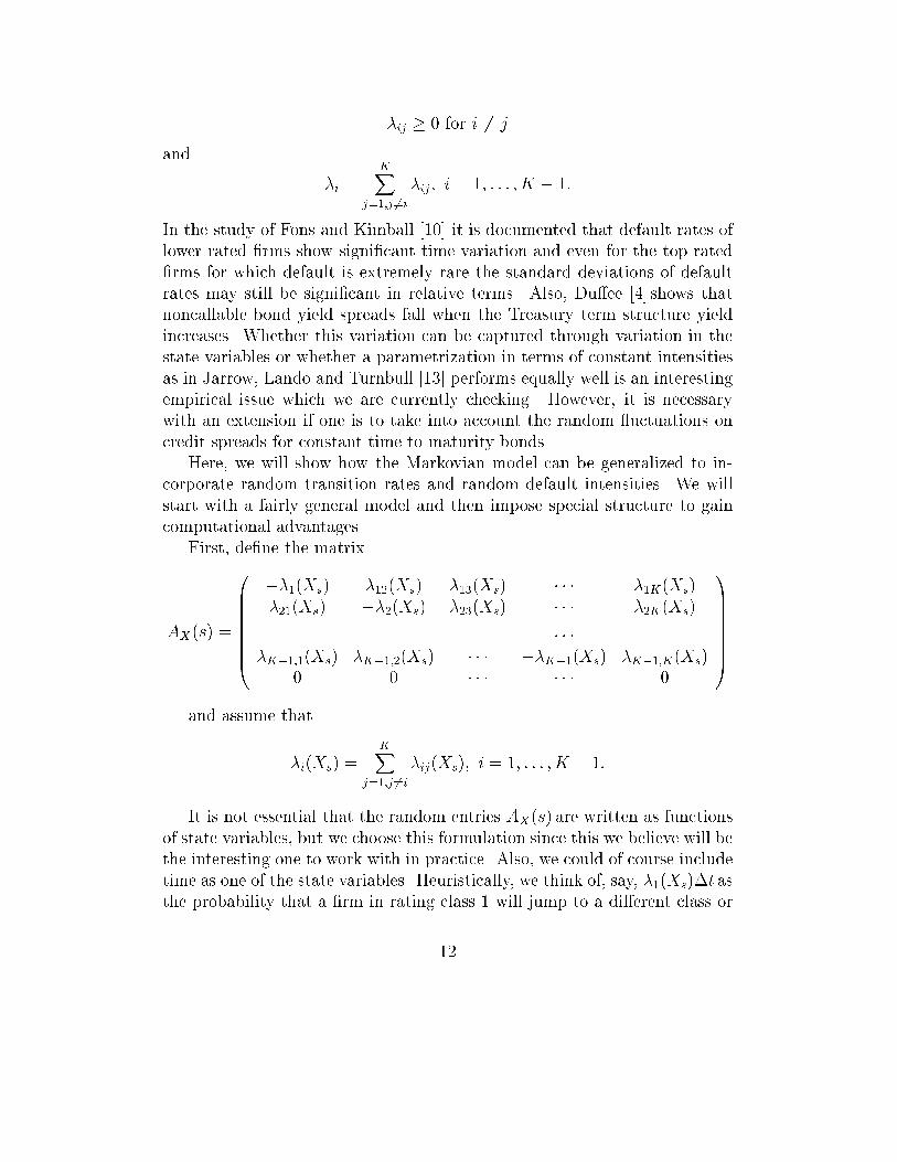
�ij � 0 for i 6= j

and

�i =KX

j=1;j 6=i

�ij; i = 1; : : : ; K � 1:

In the study of Fons and Kimball [10] it is documented that default rates of

lower rated �rms show signi�cant time variation and even for the top rated

�rms for which default is extremely rare the standard deviations of default

rates may still be signi�cant in relative terms. Also, Du�ee [4] shows that

noncallable bond yield spreads fall when the Treasury term structure yield

increases. Whether this variation can be captured through variation in the

state variables or whether a parametrization in terms of constant intensities

as in Jarrow, Lando and Turnbull [13] performs equally well is an interesting

empirical issue which we are currently checking. However, it is necessarywith an extension if one is to take into account the random uctuations on

credit spreads for constant time to maturity bonds.Here, we will show how the Markovian model can be generalized to in-

corporate random transition rates and random default intensities. We will

start with a fairly general model and then impose special structure to gaincomputational advantages.

First, de�ne the matrix

AX(s) =

0BBBBBBB@

��1(Xs) �12(Xs) �13(Xs) � � � �1K(Xs)

�21(Xs) ��2(Xs) �23(Xs) � � � �2K(Xs)...

.... . . � � �

...�K�1;1(Xs) �K�1;2(Xs) � � � ��K�1(Xs) �K�1;K(Xs)

0 0 � � � � � � 0

1CCCCCCCAand assume that

�i(Xs) =KX

j=1;j 6=i

�ij(Xs); i = 1; : : : ; K � 1:

It is not essential that the random entries AX(s) are written as functions

of state variables, but we choose this formulation since this we believe will bethe interesting one to work with in practice. Also, we could of course include

time as one of the state variables. Heuristically, we think of, say, �1(Xs)�t asthe probability that a �rm in rating class 1 will jump to a di�erent class or

12

default within the (small) time interval �t: We now give the precise mathe-

matical construction and note again that this is essential if one wants to run

simulations with the model:

Let E11; : : : ; E1K; E21; : : : ; E2K; : : : be a sequence of independent unit ex-

ponential random variables.3

Assume that a �rm starts out in rating class �0:De�ne

� �0;i = infft :Z

t

0��0;i(Xs)ds � E1ig i = 1; : : : ; K

and let

� �0 = mini6=�0

� �0;i:

Here, � �0 models the time the rating changes from the initial level �0 and

this occurs the �rst time a set of 'competing risks' which tries to pull therating away from �0 experiences a jump. The new rating level may then be

written as

�1 = argmini6=�0

� �0;i:

and if the value of �1 is K this corresponds to default. Now let

� �1;i = infft :Z

t

��0

��1;i(Xs)ds � E2ig i = 1; : : : ; K

and� �1 = min

i6=�1

� �1;i:

Hence the next jump occurs as time � �1 , the new rating level is

�2 = argmini6=�1

� �1;i

and so forth. We use � to denote the time of default, i.e.

� = inf ft : �t= Kg

With this construction we obtain a continuous time process which condi-

tionally on the evolution of the state variables is a non-homogeneous Markov

3Strictly speaking, we will only need K-1 exponentials for each jump but the notation

will be simpler by ignoring this for now.

13

chain. Conditionally on the evolution of the state variables, the transition

probabilities of this Markov chain satisfy

@PX(s; t)

@s= �AX(s)PX(s; t):

It is worth noting that the solution of this equation in the time-inhomogeneous

case is typically not equal to

PX(s; t) = exp

�Zt

s

AX(u)du

�which is most easily seen by recalling that when A and B are square matrices,

we only have

exp(A+B) = exp(A) exp(B)

when A and B commute.

For a way of writing the solution using product integral notation, see forexample of Gill and Johansen [11].

5 Pricing bonds and derivatives in the gen-

eralized Markov model

A general bond pricing formula for defaultable bonds with zero recovery isthen given in the following

Proposition 5.1 Consider a zero coupon bond maturing at time T issued

by a �rm whose rating at time t is i and whose credit rating and default

intensity evolves as described by the process � above. Then given zero recovery

in default, the price of the bond is given as

vi(t; T ) = E

exp

�Z

T

t

R(Xs)ds

!(1� PX(t; T )i;K)

�����Gt!

where PX(t; T )i;K is the (i; K)'th element of the matrix PX(t; T ):

Proof.

vi(t; T ) = B(t)Ei

1f�>Tg

B(T )

�����Ft

!

14

= Ei

1f�>Tg exp

�Z

T

t

R (Xs) ds

!�����Ft

!

= E

exp

�Z

T

t

R (Xs) ds

!Ei

�1f�>Tg

���GT _ Ft

������Ft

!

= E

exp

�Z

T

t

R(Xs)ds

!(1� PX(t; T )i;K)

�����Gt!

where we use the same argument as earlier to replace Ft by Gt:While this approach produces models that can easily be simulated using

the construction of the process � given above, it is of interest to derive models

which, although more restrictive in their assumptions, o�er computational

tractability and possibly even analytical solutions. One way to do this is

to impose more structure on the conditional intensity matrix such that the

expression for PX(s; t) simpli�es:

Lemma 5.2 For i = 1; : : : ; K � 1; let �i: Rd ! [0;1) be a non-negative

function de�ned on the state space of X and assume that for almost every

sample path of X; we have ZTf

0�i(Xs)ds <1:

Let �(Xs) denote the K�K diagonal matrix diag(�1(Xs); : : : ; �K�1(Xs); 0):For

each path of X assume that the time dependent generator matrix has the rep-

resentation

AX(s) = B�(Xs)B�1;

where B is a K � K matrix whose columns consist of K eigenvectors of

AX(s):Also, de�ne the diagonal matrix

EX(s; t) =

0BBBBBB@exp

�Rt

s�1(Xu)du

�0 � � � 0

0. . . � � � 0

... � � � exp�R

t

s�K�1(Xu)du

�0

0 � � � 0 1

1CCCCCCAThen with PX(s; t) = BEX(s; t)B

�1; PX(s; t) satis�es Kolmogorov's back-

ward equation@PX(s; t)

@s= �AX(s)PX(s; t)

15

and PX(s; t) is the transition probability of an (inhomogeneous) Markov chain

on f1; : : : ; Kg:

Proof.

Since

AX(s)B = B�X(s)

we see that

@PX(s; t)

@s= B(��

X(s))EX(s; t)B

�1

= �AX(s)BEX(s; t)B�1

= �AX(s)PX(s; t)

which shows that PX(s; t) is indeed a solution to the backward equation.From section 4.4 in Gill and Johansen [11] we know that under our assump-tions on AX(s) this equation has a unique solution, and the solution is a

transition matrix for an inhomogeneous Markov chain with the density ofthe 'intensity measure' given by AX(s): Hence PX(s; t) de�nes a Markovchain, as was to be shown.

The assumption that the eigenvectors of AX(s) exist and are not timevarying is a strong assumption. The simpli�cation is, however, profound as

well as we see in the next result which delivers a bond pricing model whichmodels bonds of all credit categories simultaneously:

Proposition 5.3 Assume that transitions between rating classes condition-

ally on X are governed by the generator matrix

AX(s) = B�(Xs)B�1

where B and �(Xs) are de�ned as in Lemma 5.2. Assume in addition, that

the K 0th row of AX(s) is 0 (corresponding to the state of default being an

absorbing state). The spot rate process for default free debt is given by R(X):

The price at time t of a zero coupon bond with maturity T , issued by a �rm

in rating class i and (for simplicity) with zero recovery in default is given by

vi(t; T ) =K�1Xj=1

�ijE

exp

ZT

t

��j(Xu)� R (Xu) du

�!�����Gt!

where the coe�cients �ijare de�ned below.

16

Proof. Conditionally on X the probability of defaulting before T given a

credit rating of i at time t (and hence no previous default since default in

this model is an absorbing state) is equal to the (i; K)0th entry of the matrix

PX(t; T ): This entry has the form

PX(t; T )i;K =KXj=1

bij exp(Z

T

t

�j(Xu)du)b

�1jK;

where b�1jK

denotes the (j;K)0th entry of B�1 and using the fact that the rows

of AX sum to 0 and that the last row of AX is 0; one may check that biKb�1KK

=

1: De�ning �ij= �bijb

�1jK

we may therefore write the probability of no default

as

1� PX(t; T )i;K =K�1Xj=1

�ijexp(

ZT

t

�j(Xu)du) (5.1)

Let superscript i on the expectation operator signify a time t rating of theissuer of i: The superscript is removed when the expectation does not depend

on this information. Now combine Proposition 5.1 and (5.1) to obtain

vi(t; T ) =K�1Xj=1

�ijE

exp

ZT

t

��j(Xu)� R (Xu) du

�!�����Gt!

We have expressed the price of bond in credit class i as a linear combi-nation of functionals of the form

E exp

�Zt

0

��j(Xu)�R (Xu) du

��:

Note that by using the results on a�ne term structure models (letting � andR be a�ne functions of di�usions with a�ne drift and volatility) we obtain

here a class of models whose bond prices are expressed as sums of a�nemodels.

To keep the exposition simple we have looked at zero coupon bonds with

zero recovery. The models above, however, also allow us to price more com-plicated contracts whose contractual payo� are linked to the rating of the

issuer. Examples include credit options and swaps with credit triggers. This

exercise can be carried out for all the three building blocks that we pricedin Section 3. Consider an example linked to credit insurance in which the

holder of the contingent claim receives a payment which depends on statevariables and on the rating of some company at a �xed time T: Here, the

17

contract itself need not have any credit risk in that it may easily pay out

an amount in the event of default of the �rm whose rating determines the

payout.

Proposition 5.4 Let the model be as in the previous proposition. Consider

a contingent claim whose payo� at time T is given as

CT = C(XT ; �T ):

Assume that the rating at time t of the �rm under consideration is i: The

price of this claim at time t is given by

Ci

t=

KXm=1

KXk=1

E

bikb

�1kmC(XT ; m) exp

ZT

t

(�k(Xu)�R (Xu) du)

!�����Gt!:

Proof. First, note that

PX(t; T )i;m =KXk=1

bikb�1km

exp(Z

T

t

�k(Xu)du);

and therefore

Ci

t= Ei

KX

m=1

C(XT ; m)PX(t; T )i;m exp

�Z

T

t

R (Xu) du

!�����Gt!

= E

KX

m=1

C(XT ; m)PX(t; T )i;m exp

�Z

T

t

R (Xu) du

!�����Gt!

= E

KX

m=1

C(XT ; m)KXk=1

bikb�1km

exp(Z

T

t

�k(Xu)du) exp

�Z

T

t

R (Xu) du

!�����Gt!

=KX

m=1

KXk=1

E

bikb

�1kmC(XT ; m) exp

ZT

t

(�k(Xu)�R (Xu) du)

!�����Gt!

which is the desired result.Note that this pricing formula allows payments to be directly linked to

the rating status of a certain risky �rm.Clearly, the parametric assumptions we impose to get the very tractable

model above are strong. By stochastic scaling of the eigenvectors we allow

stochastic changes the (K � 1)2 transition and default intensities to vary in

a K � 1 dimensional subspace and this will allow stochastic uctuations to

18

a�ect higher rated and lower rated �rms di�erently. Empirical analysis of

this form is currently being carried out in separate work.

Allowing the generator to be speci�ed more freely will complicate com-

putation but simulation is by no means the only way out: Consider again

the equation@PX(s; t)

@s= �AX(s)PX(s; t):

To compute the matrix PX(s; t); use the approximation based on a partition

s = s0 < s1 < : : : < sn = t. Then de�ne recursively

PX(t; t) = I and

PX(si; t) = PX(si+1; t)� AX(si+1)PX(si+1; t)(si � si+1) i = 0; : : : ; n� 1:

The entries in this approximation will all be functions of values of the process

X at n+1distinct values, which again brings us back to a standard numericalproblem involving only the di�usion X :

6 Fitting spreads and spread sensitivities

We consider in this section an illustrative implementation of the generalizedMarkovian model presented above. A full implementation and testing of themodels will be the topic of subsequent work and therefore the chosen param-

eters and prices should be seen primarily as illustrative and as providing away for the reader to check the calibration procedure.

The goal is to show how the generalized model building on a Vasicekmodel of the riskless term structure can be adapted in the approach usingmodi�ed eigenvalues of the generator matrix to produce a model which �ts

short credit spreads and changes in short spreads as a function of changesin the short rate for all credit classes simultaneously. The generalization to

multifactor models with a�ne structure will be apparent.Assume that the spot rate process for riskless debt is given as

drs = b(a� rt)dt+ �dBt:

Now calibrate the model to data by performing the following steps:

1. Estimate an empirical generator matrix A and assume that there exists

a matrix B whose columns are the eigenvectors of A:

19

2. Let

�j(rs) =

j+ �jrs; j = 1; : : : ; K � 1

where j; �j are constants.

3. Let �(rs) denote a K �K diagonal matrix whose �rst K � 1 diagonal

elements are given as above and with the last diagonal element equal

to zero. De�ne

AX(s) = B�(rs)B�1:

4. Choose the parameters ( j; �j)j=1;:::;K�1 such that 'two characteristics'

of each yield curve are satis�ed simultaneously across credit classes.

An example follows shortly.

By this speci�cation of the generator we may encounter negative tran-

sition intensities but just as we may choose to work with Gaussian interestrates as an approximation, despite the fact that this means negative interestrates with positive probability, we will allow the approximation of the de-

fault intensity under the risk neutral measure to be negative with positiveprobability. The constants will be chosen in practice such that the intensitiesare negative with very small probability.

In our example we work with spot spreads and sensitivities in the spotspreads to changes in r as the characteristics we wish to match. This choice

has the advantage of producing a simple linear equation to determine and�: To see this, consider the expression for the prices at time 0 of defaultablebonds with zero recovery in this special setup:

vi(t; T ) =K�1Xj=1

�ijE

exp

ZT

t

j+ �jrs � rsds

!�����Gt!

=K�1Xj=1

�ijE

exp

ZT

t

j� (1� �j)rsds

!�����Gt!:

De�ne the spot spread for class i as

si(rt) = limT!t

�

@

@Tlog vi(t; T )

!� rt:

Now we �nd

20

Proposition 6.1

si(rt) = �K�1Xj=1

�ij�j(rt)

@

@rtsi(rt) = �

K�1Xj=1

�ij�j:

Proof. Note that

�@

@Tlog vi(t; T )

=�1

vi(t; T )

@

@Tvi(t; T )

=�1

vi(t; T )

K�1Xj=1

�ijE

� j+ (�j � 1)rT

�exp

ZT

t

j+ �jrs � rsds

!�����Gt!

!T!t

K�1Xj=1

��ij

� j+ (�j � 1)rt

�

and using the fact thatP

K�1j=1 �

ij= 1 we �nd after subtracting the spot rate

that the spread is

si(rt) =K�1Xj=1

��ij

� j+ �jrt

�where in the last limit argument we use dominated convergence for condi-tional expectations. Now di�erentiate this expression to obtain

@

@rtsi(rt) = �

K�1Xj=1

�ij�j

so � determines the spread sensitivity to changes in the spot rate.

Assume that we observe at time 0 when the level of interest rates is r0; a

vector of spot yield spreads given by the vector

bs0 = �bs1(r0); : : : ; bsK�1(r0)�and that we have estimated a vector of sensitivities given by

cds0 = �cds1(r0); : : : ;cdsK�1(r0)� :21

As a consequence of the proposition, if we can calibrate our model to having

the correct spread initially and the correct sensitivities by solving the systems

��( + �r0) = bs0��� = cds0

where

� =��ij

�i;j=1;:::;K�1

� = (�1; : : : ; �K�1) and

= ( 1; : : : ; K�1):

We give an illustrative example:

In Jarrow, Lando and Turnbull [13] the generator matrix is given by

A =

0BBBBBBBBBBBBB@

�0:1153 0:1019 0:0083 0:0020 0:0031 0:0000 0:0000 0:00000:0091 �0:1043 0:0787 0:0105 0:0030 0:0030 0:0000 0:00000:0010 0:0309 �0:1172 0:0688 0:0107 0:0048 0:0000 0:0010

0:0007 0:0047 0:0713 �0:1711 0:0701 0:0174 0:0020 0:00490:0005 0:0025 0:0089 0:0813 �0:2530 0:1181 0:0144 0:0273

0:0000 0:0021 0:0034 0:0073 0:0568 �0:1928 0:0479 0:07530:0000 0:0000 0:0142 0:0142 0:0250 0:0928 �0:4318 0:28560:0000 0:0000 0:0000 0:0000 0:0000 0:0000 0:0000 0:0000

1CCCCCCCCCCCCCAAssuming a Vasicek model under the risk neutral measure with parame-

ters

a = 0:05

b = 0:01

� = 0:015

r0 = 0:05

Let the spreads in basis points for classes AAA down to CCC be givenas4

bs0 = (16; 20; 27; 44; 89; 150; 255)

4These spreads are consistent with JP Morgan's CreditMetrics estimates for spreads of

Industrial bonds with maturity one year as of July 11, 1997. The spot rates will of course

slightly di�erent

22

and for the purpose of illustration let the spread sensitivities be given as5

cds0 = (�0:2;�0:3;�0:4;�0:5;�0:6;�1:0;�2:0)

With these we can calibrate the model and get estimates of (�; ):

= (�0:1745;�0:1687;�0:1175;�0:0934;�0:0831;�0:0721;�0:0325)

� = (2:8004; 2:7181; 1:8026; 1:4139; 1:2640; 1:1200; 0:5348) :

The resulting term structures of yield spreads are shown in Figure 1 and

Figure 2.

It is important to stress that this method of adjusting the eigenvalues,

while convenient because of preserving closed-form solutions, is problematic

in the sense that one cannot be sure that desirable stochastic monotonicity

properties of the rating and default process are preserved. Therefore, wheninserting the estimated parameters into the pricing relation, the yield curves

of di�erent rating categories may cross. If one allows all entries of the ran-dom generator to vary freely (and not only in a space of dimension equalto set number of rating classes) this can be controlled. It is also possible

to randomize only the default intensities associated with each class in a waywhich leaves the transition intensities between non-default states �xed. This

method will give a natural way of incorporating fractional recovery ratesinto the intensities. In both cases several numerical issues arise which willbe treated in separate work.

7 Conclusion

We have laid out a framework which is convenient for analyzing �nancial in-

struments subject to credit risk through counterparty default and derivativeswhose underlying is a credit risk variable such as a credit spread. We take

into account the possible correlation between default free bonds and default

probabilities by letting interest rates and hazard rates be governed by com-

mon state variables. The main feature of the framework is that it reduces

the technical issues of modeling credit risk to the same issues we face when

modeling the ordinary term structure of interest rates. As a main application

5Both Longsta� and Schwartz [18] and Du�ee [4] �nd that spreads are negatively

correlated with the level of interest rates and that the sensitivity is stronger for lower

rated bonds.

23

we show how to generalize a model of Jarrow, Lando and Turnbull [13] to al-

low for stochastic transition intensities between rating categories. A main

application of this model is pricing of claims in which the credit rating of the

defaultable party enters explicitly. An implementation is given in a simple

one factor model in which the a�ne structure gives closed form solutions.

References

[1] Artzner, P. and F. Delbaen. Default risk insurance and incomplete

markets. Mathematical Finance, pages 187{195, 1995.

[2] Black, F. and M. Scholes. The pricing of options and corporate liabilities.

Journal of Political Economy, 3:637{654, 1973.

[3] I. Cooper and M. Martin. Default risk and derivative products. AppliedMathematical Finance, 3:53{74, 1996.

[4] Du�ee, G. Treasury yields and corporate bond yields spreads: An em-pirical analysis. Working Paper, Federal Reserve Board, WashingtonDC, 1996.

[5] Du�e, D. Dynamic Asset Pricing Theory. Princeton University Press,Princeton, New Jersey, 1992.

[6] Du�e, D. and Huang, M. Swap rates and credit quality. Journal of

Finance, 51(3):921{949, July 1996.

[7] Du�e, D. and K. Singleton. An econometric model of the term structure

of interest rate swap yields. Working Paper. Stanford University, 1995.

[8] Du�e, D. and K. Singleton. Econometric modeling of term structures

of defaultable bonds. Working Paper. Stanford University, 1995.

[9] Du�e, D., M. Schroder and C. Skiadas. Recursive valuation of default-able securities and the timing of resolution of uncertainty. The Annals

of Applied Probability, 6(4):1075{1090, 1996.

[10] Fons, J. and A. Kimball. Corporate bond defaults and default rates

1970-1990. The Journal of Fixed Income, pages 36{47, June 1991.

24

[11] Gill, R. and S. Johansen. A survey of product-integration with a view

towards applications in survival analysis. The Annals of Statistics,

18(4):1501{1555, 1990.

[12] Grandell, J. Doubly Stochastic Poisson Processes, volume 529 of Lecture

Notes in Mathematics. Springer, New York, 1976.

[13] Jarrow, R. and Lando D. and S. Turnbull. A markov model for the term

structure of credit risk spreads. Review of Financial Studies, 10(2):481{

523, 1997.

[14] Jarrow, R. and S. Turnbull. Pricing options on �nancial securities sub-

ject to credit risk. Journal of Finance, pages 53{85, March 1995.

[15] Karatzas, I. and S. Shreve. Brownian Motion and Stochastic Calculus.Springer, New York, 1988.

[16] Lando, D. Three essays on contingent claims pricing. PhD Dissertation,Cornell University, 1994.

[17] Lando, D. Modelling bonds and derivatives with credit risk. In M. Demp-

ster and S. Pliska, editors, Mathematics of Financial Derivativces, pages369{393. Cambridge University Press, 1997.

[18] Longsta�, F. and E. Schwartz. A simple approach to valuing risky �xedand oating rate debt. Journal of Finance, pages 789{819, July 1995.

[19] Madan, D. and H. Unal. Pricing the risks of default. Working Paper,

University of Maryland, 1995.

[20] Merton, R.C. On the pricing of corporate debt: The risk structure of

interest rates. Journal of Finance, 2:449{470, 1974.

[21] Williams, D. Probability with Martingales. Cambridge University Press,1991.

25

Yield spreads for investment grade debt after calibration

Time to maturity

Yie

ld s

prea

d in

per

cent

0 2 4 6 8 10

0.2

0.3

0.4

0.5

0.6

0.7

A

BBB

AA

AAA

Figure 1: Yield spreads on defaultable zero coupon bonds as a functionof time to maturity for investment grade ratings. The yields have been

calibrated using an empirically observed generator and a risk-adjustment tomatch both observed spot spreads and changes in spot spreads due to changes

in short treasury rates.

26

Yield spreads for speculative grade debt after calibration

Time to maturity

Yie

ld s

prea

d in

per

cent

0 2 4 6 8 10

1.0

1.5

2.0

2.5

B

CCC

BB

Figure 2: Yield spreads on defaultable zero coupon bonds as a functionof time to maturity for speculative grade ratings. The yields have been

calibrated using an empirically observed generator and a risk-adjustment tomatch both observed spot spreads and changes in spot spreads due to changes

in short treasury rates.

27