ON RANDOM EVENT DETECTION

WITH WIRELESS SENSOR NETWORKS

A Thesis

Presented in Partial Fulfillment of the Requirements for

the Degree Master of Science in the

Graduate School of The Ohio State University

By

Prabal Kumar Dutta, B.S.E.C.E.

* * * * *

The Ohio State University

2004

Master’s Examination Committee:

Anish K. Arora, Adviser

Steven B. Bibyk, Adviser

Benjamin A. Coifman

Approved by

Adviser

Department of Electricaland Computer Engineering

c© Copyright by

Prabal Kumar Dutta

2004

ABSTRACT

Wireless sensor networks hold great promise as an enabling technology for a variety

of applications. Data collection and event detection are two such classes of applica-

tions that are broadly representative and which have received considerable attention

in the literature. While wireless multi-hop data collection has achieved operational

lifetimes on the order of a year, we are unaware of lifetimes exceeding a few days or

weeks for wireless multi-hop event detection sensor networks.

Our thesis is that sensor networks for event detection are constrained by two fac-

tors which do not similarly affect data collection sensor networks. The first factor is

that no appropriate sensing, signal conditioning, and signal processing architecture

has been broadly implemented to support event detection in distributed systems that

are simultaneously energy, space, time, and message complexity-constrained. The

second factor is that middleware for services such as time synchronization, localiza-

tion, and routing are predominantly and unnecessarily proactive. A comparison of

data collection and event detection will serve to illustrate the subtle but important

differences between these applications.

Fundamentally, data collection is a signal reconstruction problem in which the

objective is to centrally reconstruct observations of distributed phenomena with high

spatial and temporal fidelity. Performance metrics for such applications include the

ii

accuracy and precision of the signal reconstruction, the correlation between the ob-

served signal and the underlying physical phenomena, and the lifetime of the sensor

network. Physical phenomena such as light, temperature, humidity, and barometric

pressure change at very low frequencies and can be sampled faithfully at periods of

a minute or more. System performance can be adjusted by introducing compression

and aggregation, or by varying the duty-cycle, sampling and communication rates,

allowing sensor lifetimes to approach a year or more.

In contrast with data collection, sensor network applications for event detection

must continuously observe noise for the rare presence of a burst of high-frequency

signal. The requirements for this style of event detection, called “passive vigilance,”

imply a sensing, signal conditioning, and signal processing architecture quite different

from that employed for the data collection problem. Fundamentally, event detection is

a signal detection problem in which the objective is to decide between two hypotheses,

or more generally a parameter estimation and pattern classification problem in which

the objective is to extract feature vectors from the signals and assign class labels to

the observed events. Performance metrics for such applications include probabilities

of detection, false alarm, classification and mis-classification, detection latency, and

lifetime of the sensor network. For many types of targets, the signals of interest may

be present for durations on the order of a second and with spectral content ranging

from 1Hz to 10kHz.

This thesis addresses the problem of how sensor networks for event detection can

exhibit lifetimes comparable to sensor networks for data collection when the former

must monitor much higher frequency signals than the latter. Part of the solution

lies the relative rates of sampling and communications and part of the solution lies

iii

in rearchitecting the sensing and signal processing hardware and software for hierar-

chical detection with always-on, low-power wakeup sensors occupying the lowest tier.

Such an architecture extends the event-centric approach into analog electronics and

augments sampling-based digital signal processing with an interrupt-driven trigger.

This work draws on experiences from one short-lived, medium scale, event detecting

sensor network implementation to design the sensing, signal conditioning, and sig-

nal processing architecture and make middleware recommendations for a long-lived,

extremely large scale, event detecting sensor network.

This thesis considers wireless sensor node design issues broadly and the sensing

and signal processing required for passive vigilance more deeply. Analysis, design,

and simulation of several generations of motes and sensorboards is presented, and

the case for a new platform is made largely on the basis of sensing and reliabil-

ity needs. Requirements representative of typical intrusion detection systems are

discussed. Sample target phenomenologies for civilians, soldiers, and vehicles are

developed. Packaging considerations are discussed. Detailed schematics, drawings,

and datasets are provided in the hope that the contributions of this thesis provide a

foundation to accelerate the development of future sensor network platforms.

iv

ON RANDOM EVENT DETECTION

WITH WIRELESS SENSOR NETWORKS

By

Prabal Kumar Dutta, M.S.

The Ohio State University, 2004

Anish K. Arora, Adviser

Steven B. Bibyk, Adviser

Wireless sensor networks hold great promise as an enabling technology for a variety

of applications. Data collection and event detection are two such classes of applica-

tions that are broadly representative and which have received considerable attention

in the literature. While wireless multi-hop data collection has achieved operational

lifetimes on the order of a year, we are unaware of lifetimes exceeding a few days or

weeks for wireless multi-hop event detection sensor networks.

Our thesis is that sensor networks for event detection are constrained by two fac-

tors which do not similarly affect data collection sensor networks. The first factor is

that no appropriate sensing, signal conditioning, and signal processing architecture

has been broadly implemented to support event detection in distributed systems that

are simultaneously energy, space, time, and message complexity-constrained. The

1

second factor is that middleware for services such as time synchronization, localiza-

tion, and routing are predominantly and unnecessarily proactive. A comparison of

data collection and event detection will serve to illustrate the subtle but important

differences between these applications.

Fundamentally, data collection is a signal reconstruction problem in which the

objective is to centrally reconstruct observations of distributed phenomena with high

spatial and temporal fidelity. Performance metrics for such applications include the

accuracy and precision of the signal reconstruction, the correlation between the ob-

served signal and the underlying physical phenomena, and the lifetime of the sensor

network. Physical phenomena such as light, temperature, humidity, and barometric

pressure change at very low frequencies and can be sampled faithfully at periods of

a minute or more. System performance can be adjusted by introducing compression

and aggregation, or by varying the duty-cycle, sampling and communication rates,

allowing sensor lifetimes to approach a year or more.

In contrast with data collection, sensor network applications for event detection

must continuously observe noise for the rare presence of a burst of high-frequency

signal. The requirements for this style of event detection, called “passive vigilance,”

imply a sensing, signal conditioning, and signal processing architecture quite different

from that employed for the data collection problem. Fundamentally, event detection is

a signal detection problem in which the objective is to decide between two hypotheses,

or more generally a parameter estimation and pattern classification problem in which

the objective is to extract feature vectors from the signals and assign class labels to

the observed events. Performance metrics for such applications include probabilities

of detection, false alarm, classification and mis-classification, detection latency, and

2

lifetime of the sensor network. For many types of targets, the signals of interest may

be present for durations on the order of a second and with spectral content ranging

from 1Hz to 10kHz.

This thesis addresses the problem of how sensor networks for event detection can

exhibit lifetimes comparable to sensor networks for data collection when the former

must monitor much higher frequency signals than the latter. Part of the solution

lies the relative rates of sampling and communications and part of the solution lies

in rearchitecting the sensing and signal processing hardware and software for hierar-

chical detection with always-on, low-power wakeup sensors occupying the lowest tier.

Such an architecture extends the event-centric approach into analog electronics and

augments sampling-based digital signal processing with an interrupt-driven trigger.

This work draws on experiences from one short-lived, medium scale, event detecting

sensor network implementation to design the sensing, signal conditioning, and sig-

nal processing architecture and make middleware recommendations for a long-lived,

extremely large scale, event detecting sensor network.

This thesis considers wireless sensor node design issues broadly and the sensing

and signal processing required for passive vigilance more deeply. Analysis, design,

and simulation of several generations of motes and sensorboards is presented, and

the case for a new platform is made largely on the basis of sensing and reliabil-

ity needs. Requirements representative of typical intrusion detection systems are

discussed. Sample target phenomenologies for civilians, soldiers, and vehicles are

developed. Packaging considerations are discussed. Detailed schematics, drawings,

and datasets are provided in the hope that the contributions of this thesis provide a

foundation to accelerate the development of future sensor network platforms.

3

Dedicated to my father, who would have been thrilled that I returned to the

academe, surprised that it took me so long to find my way, and correct that I have

always belonged here. I am forever in your debt for the sacrifices you made to give

me this opportunity. I just wish I could have told you in the living years. . .

v

This thesis would not have been possible without the support and guidance of

family, friends, colleagues, and mentors. I am lucky to be surrounded by such re-

markable and wonderful people. My deepest and most heartfelt gratitude goes out

to each of you.

Anish Arora and Steve Bibyk, my advisors, contributed countless hours of their

precious time to advise me on research, teaching, writing, collaboration, and life. I

could not have asked for greater support, encouragement, or friendship.

Anish taught me that asking the right question was more important than answer-

ing it and that the simplest questions sometimes lead to the most profound of answers.

The high expectations he has of his students are met only by his still higher commit-

ment to them. Anish is always willing to take time out of his exceptionally packed

schedule to discuss a paper, review an algorithm, or help run an experiment. He

demonstrated unusual faith and latitude with me: encouraging me to attend many

meetings, workshops and conferences, and supporting me during my semester-long

visit to U.C. Berkeley.

Steve is always so far ahead of the curve that it is difficult to grasp the gravity of

his insights. It was he who originally introduced me to the field of sensor networks

long before it was in vogue. I wish I had been able to appreciate his vision back then.

He provided many nuggets of practical advice which helped me navigate through

graduate school with little friction. Steve suggested many ideas in circuits, signal

processing, and information theory which shaped my thesis work. His guidance and

friendship know no bounds.

vi

Benn Coifman, who introduced me to the fascinating world of traffic engineering,

taught me how to efficiently manipulate and filter large volumes of data, and served

on my masters committee.

Yuan Zheng and David Orin, without whose encouragement and support I would

not have returned to graduate school.

Paul Sivilotti, whose engaging approach to education excited me so much that I

returned to graduate school after several years in industry.

Ted Herman, who helped me discover experimental computer science and made me

feel comfortable thinking of myself as an experimental computer scientist in training.

Santosh Kumar, Sandip Bapat, Vinayak Naik, Vinod Kulathumani, Hongwei

Zhang, Hui Caoh, Murat Demirbas, Mahesh Arumugam, and Young-Ri Choi, my

fellow students working on the DARPA NEST program at Ohio State, Michigan

State, and University of Texas at Austin, whose innumerable contributions made the

work described here meaningful.

Mike Grimmer, from Crossbow Technology, and Gary Myers, a long-time friend

and mentor, who provided the engineering wind beneath my research wings. Thank

you for helping keep my feet planted firmly on the ground even while I kept reaching

for the stars.

David Culler and Shankar Sastry, who were supportive of my interest to visit U.C.

Berkeley, helped make me feel at home while there, and exhibited great faith in me

when little was justified.

Sarah Bergbreiter, Cory Sharp, Robert Szewczyk, Alec Woo, Phil Levis, Joe Po-

lastre, David Molnar, and Rodrigo Fonseca, each of whom contributed to making my

visit to U.C. Berkeley in the fall of 2003 a wonderful and enriching experience.

vii

Feng Zhao and Jie Liu, who invited me to spend the summer of 2004 at Microsoft

Research, where I was exposed to a constant stream of new ideas. Seattle, a magical

city with which I fell in love, is where I wrote much of this thesis.

Alpa Shah, Elaine Cheong, Kamin Whitehouse, Naveen Sastry, AJ Shankar, and

Manu Sridharan, who are surely a large part of the reason I fell in love with Seattle.

The writing of this thesis surely would have gone much faster had I not known you,

but then again the summer surely would have been much less memorable. You made

bringing my camera along worth it.

Ethan Stock and Andrea Reichert, for taking me into their lives, introducing me

to innumerable Northern California activities, and being the kind of friends that

everyone should be so lucky to have.

Carleen and Craig Calcaterra, who kept me sane with their friendship, humor,

and wisdom for more years than I can remember. I hope the future brings as many

New Year’s Eve nights togther as the past.

And most of all, my mother, Malini, and Wendy, each of whom sacrified the one

thing they value most – our time together – so that I could write this thesis.

P.K.D.

Redmond, Washington

viii

VITA

May 24, 1974 . . . . . . . . . . . . . . . . . . . . . . . . . . . . . . . Born - Calcutta, India

1997 . . . . . . . . . . . . . . . . . . . . . . . . . . . . . . . . . . . . . . . .B.S.E.C.E.,The Ohio State University

1997 - 1998 . . . . . . . . . . . . . . . . . . . . . . . . . . . . . . . . .CTO,Bamboo Systems, Inc.,Santa Clara, California

1998 - 2002 . . . . . . . . . . . . . . . . . . . . . . . . . . . . . . . . .Co-Founder and CEO,NetEnabled, Inc.,Columbus, Ohio

2002 - present . . . . . . . . . . . . . . . . . . . . . . . . . . . . . . Graduate Student,The Ohio State University,Columbus, Ohio

PUBLICATIONS

Research Publications

A. Arora, P. Dutta, S. Bapat, V. Kulathumani, H. Zhang, V. Naik, V. Mittal, H.Cao, M. Gouda, Y. Choi, T. Herman, S. Kulkarni, U. Arumugam, M. Nesterenko, A.Vora, and M. Miyashita, “Line in the Sand: A Wireless Sensor Network for TargetDetection, Classification, and Tracking,” Computer Networks Journal, Elsevier, 2004

R.J. Freuler, M.J. Hoffman, T.P. Pavlic, J.M. Beams, J.P. Radigan, P.K. Dutta, J.T.Demel, and E.D. Justen, “Experiences with a Freshman Capstone Course - Designing,Building, and Testing Small Autonomous Robots,” Proceedings of the 2003 AmericanSociety for Engineering Education Annual Conference & Exposition, 2003

A.W. Fentiman, J.T. Demel, R. Boyd, K. Pugsley, P. Dutta, “Helping Students Learnto Organize and Manage a Design Project,” Proceedings of the American Society forEngineering Education Annual Conference, 1996

ix

S.V. Sreenivasan, P.K. Dutta, K.J. Waldron, “The Wheeled Actively ArticulatedVehicle (WAAV): An Advanced Offroad Mobility Concept,” Advances in Robot Kine-matics and Computational Geometry, J. Lenarcic, B. Ravani, Eds., Kluwer AcademicPublishers, 1994

FIELDS OF STUDY

Major Field: Electrical and Computer Engineering

Studies in:

Electrical Engineering Prof. Steven B. BibykComputer Science Prof. Anish K. Arora

x

TABLE OF CONTENTS

Page

Abstract . . . . . . . . . . . . . . . . . . . . . . . . . . . . . . . . . . . . . . . ii

Dedication . . . . . . . . . . . . . . . . . . . . . . . . . . . . . . . . . . . . . . v

Vita . . . . . . . . . . . . . . . . . . . . . . . . . . . . . . . . . . . . . . . . . ix

List of Tables . . . . . . . . . . . . . . . . . . . . . . . . . . . . . . . . . . . . xvi

List of Figures . . . . . . . . . . . . . . . . . . . . . . . . . . . . . . . . . . . xvii

Chapters:

1. Introduction . . . . . . . . . . . . . . . . . . . . . . . . . . . . . . . . . . 1

1.1 Motivation . . . . . . . . . . . . . . . . . . . . . . . . . . . . . . . 21.2 Overview . . . . . . . . . . . . . . . . . . . . . . . . . . . . . . . . 41.3 Organization . . . . . . . . . . . . . . . . . . . . . . . . . . . . . . 8

2. Random Event Detection . . . . . . . . . . . . . . . . . . . . . . . . . . . 10

2.1 Related Work . . . . . . . . . . . . . . . . . . . . . . . . . . . . . . 112.2 The Nature of Random Events . . . . . . . . . . . . . . . . . . . . 132.3 A Comparison of Applications . . . . . . . . . . . . . . . . . . . . . 15

2.3.1 Key Differences . . . . . . . . . . . . . . . . . . . . . . . . . 152.3.2 Energy Usage Profiles . . . . . . . . . . . . . . . . . . . . . 19

2.4 A Candidate Architecture . . . . . . . . . . . . . . . . . . . . . . . 212.4.1 Low-Power Sensing and Processing . . . . . . . . . . . . . . 222.4.2 Hierarchy . . . . . . . . . . . . . . . . . . . . . . . . . . . . 232.4.3 Reactive Middleware . . . . . . . . . . . . . . . . . . . . . . 24

xi

3. The eXtreme Scale Mote (XSM) . . . . . . . . . . . . . . . . . . . . . . . 27

3.1 Related Work . . . . . . . . . . . . . . . . . . . . . . . . . . . . . . 283.1.1 Applications . . . . . . . . . . . . . . . . . . . . . . . . . . 283.1.2 Platforms . . . . . . . . . . . . . . . . . . . . . . . . . . . . 303.1.3 Circuits . . . . . . . . . . . . . . . . . . . . . . . . . . . . . 31

3.2 Application Requirements . . . . . . . . . . . . . . . . . . . . . . . 323.2.1 Functionality . . . . . . . . . . . . . . . . . . . . . . . . . . 323.2.2 Usability . . . . . . . . . . . . . . . . . . . . . . . . . . . . 333.2.3 Reliability . . . . . . . . . . . . . . . . . . . . . . . . . . . . 343.2.4 Performance . . . . . . . . . . . . . . . . . . . . . . . . . . 353.2.5 Supportability . . . . . . . . . . . . . . . . . . . . . . . . . 36

3.3 Platform . . . . . . . . . . . . . . . . . . . . . . . . . . . . . . . . 373.3.1 Processor . . . . . . . . . . . . . . . . . . . . . . . . . . . . 383.3.2 Radio . . . . . . . . . . . . . . . . . . . . . . . . . . . . . . 393.3.3 Grenade Timer and Real-Time Clock . . . . . . . . . . . . . 433.3.4 Network Bootloader . . . . . . . . . . . . . . . . . . . . . . 503.3.5 User Interface . . . . . . . . . . . . . . . . . . . . . . . . . . 52

3.4 Sensors . . . . . . . . . . . . . . . . . . . . . . . . . . . . . . . . . 533.4.1 Acoustic . . . . . . . . . . . . . . . . . . . . . . . . . . . . . 563.4.2 Magnetic . . . . . . . . . . . . . . . . . . . . . . . . . . . . 603.4.3 Passive Infrared . . . . . . . . . . . . . . . . . . . . . . . . 603.4.4 Photo and Temperature . . . . . . . . . . . . . . . . . . . . 613.4.5 Acceleration . . . . . . . . . . . . . . . . . . . . . . . . . . 62

3.5 Power . . . . . . . . . . . . . . . . . . . . . . . . . . . . . . . . . . 623.6 Packaging . . . . . . . . . . . . . . . . . . . . . . . . . . . . . . . . 633.7 Summary . . . . . . . . . . . . . . . . . . . . . . . . . . . . . . . . 64

4. Detection and Classification of Ferromagnetic Targets . . . . . . . . . . . 68

4.1 Related Work . . . . . . . . . . . . . . . . . . . . . . . . . . . . . . 694.2 Target Model . . . . . . . . . . . . . . . . . . . . . . . . . . . . . . 704.3 Sensor Platform . . . . . . . . . . . . . . . . . . . . . . . . . . . . 73

4.3.1 Mica2 Processor and Radio Board . . . . . . . . . . . . . . 734.3.2 Mica Sensor Board . . . . . . . . . . . . . . . . . . . . . . . 73

4.4 Towards Low-power Sensing . . . . . . . . . . . . . . . . . . . . . . 744.5 Detection . . . . . . . . . . . . . . . . . . . . . . . . . . . . . . . . 784.6 Classification . . . . . . . . . . . . . . . . . . . . . . . . . . . . . . 81

4.6.1 The Influence Field as a Spatial Statistic . . . . . . . . . . . 824.6.2 Influence Field Estimator . . . . . . . . . . . . . . . . . . . 844.6.3 Classifier Design . . . . . . . . . . . . . . . . . . . . . . . . 85

xii

4.6.4 Validation . . . . . . . . . . . . . . . . . . . . . . . . . . . . 86

5. Towards UWB Radar-Enabled Sensor Networks . . . . . . . . . . . . . . 94

5.1 Introduction . . . . . . . . . . . . . . . . . . . . . . . . . . . . . . 945.2 Theory of Operation . . . . . . . . . . . . . . . . . . . . . . . . . . 965.3 Sensor Platform . . . . . . . . . . . . . . . . . . . . . . . . . . . . 99

5.3.1 Radar Sensor and Antenna . . . . . . . . . . . . . . . . . . 995.3.2 Mica Power Board . . . . . . . . . . . . . . . . . . . . . . . 1015.3.3 Mica Sensor Board . . . . . . . . . . . . . . . . . . . . . . . 1035.3.4 Mica2 Processor and Radio Board . . . . . . . . . . . . . . 1035.3.5 Packaging . . . . . . . . . . . . . . . . . . . . . . . . . . . . 103

5.4 Power Considerations . . . . . . . . . . . . . . . . . . . . . . . . . 1045.5 Detection . . . . . . . . . . . . . . . . . . . . . . . . . . . . . . . . 105

5.5.1 Signal . . . . . . . . . . . . . . . . . . . . . . . . . . . . . . 1075.5.2 Noise and Clutter . . . . . . . . . . . . . . . . . . . . . . . 1125.5.3 Energy Detector . . . . . . . . . . . . . . . . . . . . . . . . 1125.5.4 Histogram-similarity Detector . . . . . . . . . . . . . . . . . 115

6. ETA: The Elapsed Time on Arrival Protocol . . . . . . . . . . . . . . . . 122

6.1 Related Work . . . . . . . . . . . . . . . . . . . . . . . . . . . . . . 1226.2 Elapsed Time on Arrival . . . . . . . . . . . . . . . . . . . . . . . . 124

7. RARE: The ReActive Range Estimation Protocol . . . . . . . . . . . . . 127

7.1 Introduction . . . . . . . . . . . . . . . . . . . . . . . . . . . . . . 1287.1.1 Background . . . . . . . . . . . . . . . . . . . . . . . . . . . 1287.1.2 Motivation and Approach . . . . . . . . . . . . . . . . . . . 1307.1.3 Organization . . . . . . . . . . . . . . . . . . . . . . . . . . 131

7.2 Related Work . . . . . . . . . . . . . . . . . . . . . . . . . . . . . . 1317.3 Range Estimation . . . . . . . . . . . . . . . . . . . . . . . . . . . 1347.4 Distance Estimation . . . . . . . . . . . . . . . . . . . . . . . . . . 134

7.4.1 Case 1 . . . . . . . . . . . . . . . . . . . . . . . . . . . . . . 1367.4.2 Case 2 . . . . . . . . . . . . . . . . . . . . . . . . . . . . . . 1387.4.3 Ambiguities and Assumptions . . . . . . . . . . . . . . . . . 1407.4.4 Pairwise Distance Estimation Algorithm . . . . . . . . . . . 141

7.5 Implementation . . . . . . . . . . . . . . . . . . . . . . . . . . . . . 1447.5.1 Network Nodes . . . . . . . . . . . . . . . . . . . . . . . . . 1457.5.2 Ultrasound Transceiver . . . . . . . . . . . . . . . . . . . . 1467.5.3 Experimental Setup . . . . . . . . . . . . . . . . . . . . . . 146

7.6 Results . . . . . . . . . . . . . . . . . . . . . . . . . . . . . . . . . 148

xiii

7.7 Summary . . . . . . . . . . . . . . . . . . . . . . . . . . . . . . . . 1507.8 Future Work . . . . . . . . . . . . . . . . . . . . . . . . . . . . . . 152

8. Conclusions . . . . . . . . . . . . . . . . . . . . . . . . . . . . . . . . . . 155

9. Future Work . . . . . . . . . . . . . . . . . . . . . . . . . . . . . . . . . 162

9.1 Sensor and Platforms . . . . . . . . . . . . . . . . . . . . . . . . . . 1629.2 Ultrawideband Technologies . . . . . . . . . . . . . . . . . . . . . . 1649.3 Tool Support for Signal Processing . . . . . . . . . . . . . . . . . . 1649.4 Applications . . . . . . . . . . . . . . . . . . . . . . . . . . . . . . 165

Appendices:

A. Electrical Schematics . . . . . . . . . . . . . . . . . . . . . . . . . . . . . 169

A.1 Mica Power Board . . . . . . . . . . . . . . . . . . . . . . . . . . . 170A.1.1 Mica Power Board 1.0 Top View . . . . . . . . . . . . . . . 170A.1.2 Mica Power Board 1.0 Schematic . . . . . . . . . . . . . . . 171

A.2 XSM 1.0 . . . . . . . . . . . . . . . . . . . . . . . . . . . . . . . . . 172A.2.1 XSM 1.0 Top View . . . . . . . . . . . . . . . . . . . . . . . 173A.2.2 XSM 1.0 Bottom View . . . . . . . . . . . . . . . . . . . . . 174A.2.3 Acoustic Subsystem . . . . . . . . . . . . . . . . . . . . . . 175A.2.4 XSM 1.0 Power, Accelerometer, and LEDs . . . . . . . . . . 176A.2.5 XSM 1.0 Radio Subsystem . . . . . . . . . . . . . . . . . . 177A.2.6 XSM 1.0 Expansion Connector . . . . . . . . . . . . . . . . 178A.2.7 XSM 1.0 Microcontroller and Memory Subsystem . . . . . . 179A.2.8 XSM 1.0 Magnetometer Subsystem . . . . . . . . . . . . . . 180A.2.9 XSM 1.0 Passive Infrared Subsystem . . . . . . . . . . . . . 181

A.3 XSM 2.0 . . . . . . . . . . . . . . . . . . . . . . . . . . . . . . . . . 182A.3.1 XSM 2.0 Top View . . . . . . . . . . . . . . . . . . . . . . . 183A.3.2 XSM 2.0 Bottom View . . . . . . . . . . . . . . . . . . . . . 184A.3.3 XSM 2.0 Acoustic Subsystem . . . . . . . . . . . . . . . . . 185A.3.4 XSM 2.0 Power, Accelerometer, LEDs, and Grenade Timer 186A.3.5 XSM 2.0 Sounder Subsystem . . . . . . . . . . . . . . . . . 187A.3.6 XSM 2.0 Radio Subsystem . . . . . . . . . . . . . . . . . . 188A.3.7 XSM 2.0 Expansion Connector . . . . . . . . . . . . . . . . 189A.3.8 XSM 2.0 Microcontroller and Memory Subsystem . . . . . . 190A.3.9 XSM 2.0 Magnetometer Subsystem . . . . . . . . . . . . . . 191A.3.10 XSM 2.0 Passive Infrared Subsystem . . . . . . . . . . . . . 192

xiv

B. Circuit Simulations . . . . . . . . . . . . . . . . . . . . . . . . . . . . . . 193

B.1 Acoustic . . . . . . . . . . . . . . . . . . . . . . . . . . . . . . . . . 193B.2 Passive Infrared . . . . . . . . . . . . . . . . . . . . . . . . . . . . . 195

C. Packaging Concepts . . . . . . . . . . . . . . . . . . . . . . . . . . . . . . 197

C.1 Capsule . . . . . . . . . . . . . . . . . . . . . . . . . . . . . . . . . 198C.2 Hockey Puck . . . . . . . . . . . . . . . . . . . . . . . . . . . . . . 200C.3 Cone . . . . . . . . . . . . . . . . . . . . . . . . . . . . . . . . . . . 202C.4 COTS Box A . . . . . . . . . . . . . . . . . . . . . . . . . . . . . . 204C.5 COTS Box B . . . . . . . . . . . . . . . . . . . . . . . . . . . . . . 205

D. Experimental Data . . . . . . . . . . . . . . . . . . . . . . . . . . . . . . 207

D.1 Magnetometer . . . . . . . . . . . . . . . . . . . . . . . . . . . . . 207D.1.1 Procedural Considerations . . . . . . . . . . . . . . . . . . . 207D.1.2 Experimental Setup . . . . . . . . . . . . . . . . . . . . . . 210D.1.3 Experiments . . . . . . . . . . . . . . . . . . . . . . . . . . 211

D.2 Radar . . . . . . . . . . . . . . . . . . . . . . . . . . . . . . . . . . 226

E. Releases . . . . . . . . . . . . . . . . . . . . . . . . . . . . . . . . . . . . 229

Bibliography . . . . . . . . . . . . . . . . . . . . . . . . . . . . . . . . . . . . 232

xv

LIST OF TABLES

Table Page

2.1 Data collection vs event detection . . . . . . . . . . . . . . . . . . . . 16

2.2 Relating useful work to energy. . . . . . . . . . . . . . . . . . . . . . 20

3.1 Estimated current draw of XSM subsystems. . . . . . . . . . . . . . . 63

4.1 The confusion matrix for the influence field classifier . . . . . . . . . . 91

7.1 Range estimation error . . . . . . . . . . . . . . . . . . . . . . . . . . 153

xvi

LIST OF FIGURES

Figure Page

2.1 Energy profiles. . . . . . . . . . . . . . . . . . . . . . . . . . . . . . . 21

3.1 Top view of XSM. . . . . . . . . . . . . . . . . . . . . . . . . . . . . . 38

3.2 Radio output power . . . . . . . . . . . . . . . . . . . . . . . . . . . . 42

3.3 Radio-antenna junction reflections. . . . . . . . . . . . . . . . . . . . 43

3.4 Grenade timer and real-time clock. . . . . . . . . . . . . . . . . . . . 48

3.5 Sallen-Key low pass filter. . . . . . . . . . . . . . . . . . . . . . . . . 57

3.6 Sallen-Key high pass filter. . . . . . . . . . . . . . . . . . . . . . . . . 59

3.7 Bode diagram of bandpass pass filter . . . . . . . . . . . . . . . . . . 65

3.8 Frequency response of PIR circuit . . . . . . . . . . . . . . . . . . . . 66

3.9 Accelerometer circuit . . . . . . . . . . . . . . . . . . . . . . . . . . . 66

3.10 XSM enclosure. . . . . . . . . . . . . . . . . . . . . . . . . . . . . . . 67

4.1 Magnetic dipole model. . . . . . . . . . . . . . . . . . . . . . . . . . . 72

4.2 Sample-and-hold control circuit. . . . . . . . . . . . . . . . . . . . . . 76

4.3 Magnetometer signal detection chain . . . . . . . . . . . . . . . . . . 79

4.4 The shape of the influence field of a soldier and a vehicle . . . . . . . 87

xvii

4.5 The influence field of a soldier and a car as measured in situ . . . . . 89

4.6 Probability distribution of the estimated influence field . . . . . . . . 90

5.1 Radar sensor network node . . . . . . . . . . . . . . . . . . . . . . . . 100

5.2 Advantaca TWR-ISM-002 . . . . . . . . . . . . . . . . . . . . . . . . 101

5.3 Mica Power Board . . . . . . . . . . . . . . . . . . . . . . . . . . . . 102

5.4 Radar sensor node . . . . . . . . . . . . . . . . . . . . . . . . . . . . 105

5.5 Radar initialization . . . . . . . . . . . . . . . . . . . . . . . . . . . . 106

5.6 Radar waveform and spectrogram of person running . . . . . . . . . . 107

5.7 Radar waveform and spectrogram of person walking . . . . . . . . . . 108

5.8 Radar signature of person walking. . . . . . . . . . . . . . . . . . . . 109

5.9 Radar signature of person running. . . . . . . . . . . . . . . . . . . . 110

5.10 Radar signature of vehicle passing. . . . . . . . . . . . . . . . . . . . 111

5.11 Sample radar noise data . . . . . . . . . . . . . . . . . . . . . . . . . 113

5.12 Amplitude and histogram of radar noise . . . . . . . . . . . . . . . . 117

5.13 Amplitude and histogram of radar signal . . . . . . . . . . . . . . . . 118

5.14 Moving histogram over radar waveform . . . . . . . . . . . . . . . . . 121

6.1 Elapsed Time on Arrival (ETA) algorithm . . . . . . . . . . . . . . . 125

7.1 Target trajectory between the nodes. . . . . . . . . . . . . . . . . . . 135

7.2 Target trajectory not between the nodes. . . . . . . . . . . . . . . . . 136

7.3 Sensor Hardware . . . . . . . . . . . . . . . . . . . . . . . . . . . . . 145

7.4 Temporal variation of the range error over time . . . . . . . . . . . . 147

xviii

7.5 The range error distribution . . . . . . . . . . . . . . . . . . . . . . . 148

7.6 The target trajectories . . . . . . . . . . . . . . . . . . . . . . . . . . 149

7.7 Experimental Setup . . . . . . . . . . . . . . . . . . . . . . . . . . . . 150

7.8 Range estimate waveform. . . . . . . . . . . . . . . . . . . . . . . . . 151

7.9 Range estimate sum and difference . . . . . . . . . . . . . . . . . . . 152

7.10 Target trajectory . . . . . . . . . . . . . . . . . . . . . . . . . . . . . 153

8.1 Typical data collection schedule. . . . . . . . . . . . . . . . . . . . . . 159

B.1 Frequency response of microphone band pass filter circuit . . . . . . . 194

B.2 Frequency response of PIR circuit . . . . . . . . . . . . . . . . . . . . 196

C.1 Capsule enclosure. . . . . . . . . . . . . . . . . . . . . . . . . . . . . 198

C.2 Hockey puck enclosure. . . . . . . . . . . . . . . . . . . . . . . . . . . 200

C.3 Cone enclosure . . . . . . . . . . . . . . . . . . . . . . . . . . . . . . 202

C.4 Simple COTS enclosure . . . . . . . . . . . . . . . . . . . . . . . . . 204

C.5 Heavily-modified COTS enclosure . . . . . . . . . . . . . . . . . . . . 205

C.6 Heavily-modified COTS enclosure (transparent) . . . . . . . . . . . . 206

D.1 Experimental Setup. . . . . . . . . . . . . . . . . . . . . . . . . . . . 211

D.2 Velocity Experiment. . . . . . . . . . . . . . . . . . . . . . . . . . . . 214

D.3 Distance Experiment. . . . . . . . . . . . . . . . . . . . . . . . . . . . 217

D.4 Orientation Experiment. . . . . . . . . . . . . . . . . . . . . . . . . . 221

D.5 Magnetometer bias drift . . . . . . . . . . . . . . . . . . . . . . . . . 225

xix

D.6 UWB radar dataset thumbnails . . . . . . . . . . . . . . . . . . . . . 228

xx

CHAPTER 1

INTRODUCTION

Deeply embedded and densely distributed networked systems that can sense and

control the environment, perform local computations, and communicate the results

will allow us to interact with the physical world on space and time scales previ-

ously unobtainable. These sensor actuator networks or just “sensornets” became

possible with the emergence of micro electro mechanical systems (MEMS) sensors

and actuators, low-power complementary metal oxide semiconductor (CMOS) analog

and digital electronics including radios and microcontrollers, custom very large scale

integration (VLSI) circuits, and organic photovoltaic cells. While not all of these

innovations have made their way into mainstream research platforms for sensors net-

works, many of the technologies have been incorporated into commercial off-the-shelf

(COTS) platforms which have supported a groundswell of systems and applications

research.

1

1.1 Motivation

Paraphrasing Mark Weiser, the late Chief Scientist of Xerox PARC and father of

ubiquitous computing, “‘Applications are of course the whole point of’ sensor net-

working.”1 It is clear that wireless sensor networks hold great promise as an enabling

technology for a variety of applications. Habitat monitoring is one such application

that is representative of an entire class of data collection applications which have

received considerable attention in the literature. Fundamentally, data collection is

a signal reconstruction problem in which the objective is to centrally reconstruct

observations of distributed phenomena with high spatial and temporal fidelity. Per-

formance metrics for such applications include the accuracy and precision of the signal

reconstruction, the correlation between the observed signal and the underlying phys-

ical phenomena, and the lifetime of the sensor network. Physical phenomena such as

light, temperature, humidity, and barometric pressure change at very low frequencies

and can be sampled faithfully at periods of a minute or more. System performance

can be adjusted by introducing compression and aggregation, or by varying the duty-

cycle, sampling and communication rates. Using COTS platforms, researchers have

demonstrated periodic data collection applications with lifetimes on the order of a

year.

In contrast with data collection, sensor network applications like intrusion detec-

tion and military surveillance must continuously observe noise for the rare presence

of a burst of high frequency signal. The requirements for this style of application,

1Weiser actually wrote “Applications are of course the whole point of ubiquitous computing,”but many consider sensornets and ubiquitous computing to be closely related.

2

called event detection, imply a sensing and signal processing architecture quite dif-

ferent from that employed for the data collection problem. Fundamentally, intrusion

detection is a event detection problem in which the objective is to decide between

two or more hypotheses, or more generally a parameter estimation, pattern classifica-

tion, and target tracking problem in which the objective is to extract feature vectors

from the signals, assign class labels to the intruding target, and estimate its past and

future locations. Performance metrics for such applications include probabilities of

detection, false alarm, classification and mis-classification, detection latency, tracking

accuracy, and system lifetime. For many types of targets, the signals of interest may

be present for durations on the order of a second and with spectral content ranging

from 1Hz to 10kHz.

While existing sensornet platforms have enabled researchers to demonstrate long-

lived periodic data collection applications, similarly long-lived intrusion detection

and military surveillance have not, to our knowledge, surfaced. We believe that the

heretofore lack of unified platform and middleware support for passive vigilance has

been a key inhibiting factor. One bottleneck is likely due to the multi-disciplinary

nature of the field. While sensornets are often characterized as standard experimental

computer science and engineering, the design space is much broader and draws on

many aspects of electrical engineering and computer science, and at least some areas

of mechanical engineering and materials science. As a result of the unusually broad

range of backgrounds and technologies needed to field complete systems, researchers

have focused on narrower aspects of the field, and have chosen to use commercially

available platforms rather than create highly customized new ones, a few exceptions

3

notwithstanding. Building new platforms is an expensive and time consuming propo-

sition so it is not at all surprising that so few are broadly available and consequently

much of the research effort avoids platform building.

We take the opposite view: that ultimately these diverse sensors, algorithms,

platforms, radios, batteries, and other components must be assembled into cohesive

integrated systems to provide value, and that the process of actually building these

systems will teach us a great deal. Again, Mark Weiser’s words are at once prescient

and apropos: “The research method for ubiquitous computing is standard experi-

mental computer science: the construction of working prototypes of the necessary

infrastructure in sufficient quantity to debug the viability of the systems in everyday

use; ourselves and a few collegues serving as guinea pigs. This is an important step

toward ensuring that our infrastructure research is robust and scalable in the face of

the details of the real world.”

1.2 Overview

This thesis addresses the question of how sensor networks for event detection can

exhibit lifetimes comparable to sensor networks for data collection when the former

must monitor much higher frequency signals than the latter. We advocate a purely

reactive or event-driven sensing, signal processing, middleware, and communications

architecture for the detection of random events.

One aspect of the solution lies in reallocating power budgets based on the rela-

tive rates of sampling and communications. Another aspect of the solution lies in

rearchitecting the sensing and signal processing hardware and software for hierarchi-

cal detection with low-power wakeup sensors occupying the lowest tier. Most existing

4

sensor designs do not address the low-power sensing requirement for long-lived net-

works so this has led to the genesis and evolution of a novel sensor network platform

developed to investigate low-power event detection applications which require pas-

sive vigilance. A third aspect of the solution lies in reactive, or lazy, middleware for

services like time synchronization and localization.

We ground our research in the problem of intrusion detection using sensor net-

works. The instrumentation of a militarized zone with distributed sensors is a decades-

old idea, with implementations dating at least as far back as the Vietnam-era Igloo

White program [1]. Unattended ground sensors (UGS) exist today that can de-

tect, classify, and determine the direction of movement of intruding personnel and

vehicles. The Remotely Monitored Battlefield Sensor System (REMBASS) exempli-

fies UGS systems in use today [1]. REMBASS exploits remotely monitored sensors,

hand-emplaced along likely enemy avenues of approach. These sensors respond to

seismic-acoustic energy, infrared energy, and magnetic field changes to detect enemy

activities. REMBASS processes the sensor data locally and outputs detection and

classification information wirelessly, either directly or through radio repeaters, to the

sensor monitoring set (SMS). Messages are demodulated, decoded, displayed, and

recorded to provide a time-phased record of intruder activity at the SMS.

Like Igloo White and REMBASS, most of the existing radio-based unattended

ground sensor systems have limited networking ability and communicate their sensor

readings or intrusion detections over relatively long and frequently uni-directional

radio links to a central monitoring station, perhaps via one or more simple repeater

stations. Since these systems employ long communication links, they expend precious

5

energy during transmission, which in turn reduces their lifetime. For example, a

REMBASS sensor node, once emplaced, can be unattended for only 30 days.

Recent research has demonstrated the feasibility of ad hoc aerial deployments of

1-dimensional sensor networks that can detect and track vehicles. In March 2001, re-

searchers from the University of California at Berkeley demonstrated the deployment

of a sensor network onto a road from an unmanned aerial vehicle (UAV) at Twen-

tynine Palms, California, at the Marine Corps Air/Ground Combat Center. The

network established a time-synchronized multi-hop communication network among

the nodes on the ground whose job was to detect and track vehicles passing through

the area over a dirt road. The vehicle tracking information was collected from the

sensors using the UAV in a flyover maneuver and then relayed to an observer at the

base camp.

In this work, we describe a system and method to detect and classify ferromagnetic

targets. Our approach complements and improves upon existing unattended battle-

field ground sensors by replacing the typically expensive, hand-emplaced, sparsely-

deployed, non-networked, and transmit-only sensors with collaborative sensing, com-

puting, and communicating nodes. Such an approach will enable military forces

to blanket a battlefield with easily deployable and low-cost sensors, obtaining fine-

grained situational awareness enabling friendly forces to see through the “fog of war”

with precision previously unimaginable. A strategic assessment workshop organized

by the U.S. Army Research Lab concluded:

“It is not practical to rely on sophisticated sensors with large power supplyand communication [demands]. Simple, inexpensive individual devices de-ployed in large numbers are likely to be the source of battlefield awarenessin the future. As the number of devices in distributed sensing systems in-creases from hundreds to thousands and perhaps millions, the amount of

6

attention paid to networking and to information processing must increasesharply.”

The main contributions of this work are that it (i) presents an architecture and

methodology for constructing long-lived event detection applications, (ii) demon-

strates, through a proof-of-concept system implementation, that it is possible to

detect and discriminate between multiple object classes using simple low-power sen-

sors, (iii) develops low-power signal detection algorithms for processing radar signals,

(iv) presents a novel application of the sample-and-hold circuit for reducing the power

consumption of sensors, (v) develops reactive algorithms for time synchronization and

localization that are suitable for event detection, and (vi) presents empirical data on

the noise and clutter that sensor networks in real environments will need to contend

with.

This thesis addresses the problem of how sensor networks for signal detection

can exhibit lifetimes comparable to sensor networks for signal reconstruction when

the former must monitor much higher frequency signals than the latter. Part of

the solution lies the relative rates of sampling and communications and part of the

solution lies in rearchitecting the sensing and signal processing hardware and software

for hierarchical detection with low-power wakeup sensors occupying the lowest tier.

This thesis considers wireless sensor node design issues broadly and the sensing

and signal processing required for passive vigilance more deeply. Analysis, design, and

simulation of several generations of motes and sensorboards is presented, and the case

for a new platform is made largely on the basis of sensing and reliability needs. Re-

quirements representative of typical intrusion detection systems are discussed. Sample

target phenomenologies for civilians, soldiers, and vehicles are developed. Packaging

7

considerations are discussed. Device driver and system library listings are presented

and annotated. Unit, system, and network level testing strategies and applications

are presented. Detailed schematics, drawings, and datasheet references are provided

in the hope that the contributions of this thesis provide a foundation to accelerate

the development of future sensor network platforms.

Each node can send out as little as one bit of information about the presence

or absence of a target in its sensing range and only requires local detection and

estimation, but no computationally complex time-frequency domain signal processing.

1.3 Organization

Chapter 2 presents a detailed discussion about the differences between periodic

data collection and random event detection using wireless sensor networks. Chapter 3

presents the philosophy, requirements, and design of the eXtreme Scale Mote (XSM).

This new mote is an integrated application-specific sensor network node for investigat-

ing reliable, large-scale, and long-lived surveillance applications. Chapter 4 considers

low-power hardware and energy efficient algorithms for detection and classification

of ferromagnetic targets. This chapter also introduces the influence field as a spatial

statistic suitable for classification purposes. Chapter 5 investigates the suitability of

ultrawideband radar as a sensing technology for resource-constrained sensor networks

and considers sensor-specific factors like range, power, latency, interference, and size

as well as low space, time, and message complexity algorithms for signal detection,

parameter estimation, and target classification. Chapter 6 observes that by postpon-

ing the conversion of local time to global time for as long as possible, we can reduce

the energy consumed for proactive timesync. This chapter presents a simple time

8

synchronization protocol for maintaining the elapsed time from an event. Chapter 7

explores the relationship between mobility and ranging. This chapter shows that a

mobile object can aid sensor nodes in estimating the distance to neighboring nodes

and presents an algorithm to do so. Chapter 8 summarizes our results, discusses some

of the challenges and failures we encountered during the development and fielding of

this system, and provides our concluding thoughts. Chapter 9 discusses our future

plans in the areas of tools, sensors, platforms, algorithms, and applications. Finally,

the appendices present electrical schematics, circuit simulations, packaging concepts,

and selected experimental data.

9

CHAPTER 2

RANDOM EVENT DETECTION

Wireless sensor networks hold great promise as an enabling technology for a variety

of applications. Data collection and event detection are two such classes of applica-

tions that are broadly representative and which have received considerable attention

in the literature. While wireless multi-hop data collection has achieved operational

lifetimes on the order of a year or more, we are unaware of lifetimes exceeding a few

days or weeks for wireless multi-hop event detection using sensor networks. Our key

observation is that the detection of random events is a fundamentally different prob-

lem from the periodic collection of data and that these differences give rise to a rich

space of tradeoffs and a multitude of opportunities for energy savings. For example,

data collection may allow sensor nodes to sleep most of the time but event detection

requires that sensors be vigilant most of the time. On the other hand, data collection

may require frequent messaging to report measurements but event detection may only

require reporting when an event actually occurs. In the case of sensing, data collec-

tion is more miserly with energy but in the case of messaging, event detection may

be more miserly with energy. Grounded in our experiences from two sensor network

deployments for detecting, classifying, and tracking intruding civilians, soldiers, and

10

vehicles, we present a set of design considerations and implications for the general

class of event detection applications.

2.1 Related Work

A number of earlier works have recognized and addressed some of unique char-

acteristics of event detection, as well as the differences between event detection and

data collection. In, [2] and [3], Pottie, et.al. identify tradeoffs in detection and com-

munications, ideas for network management, and scalable network architectures. The

first of the two papers identifies the important question of hierarchy of signal process-

ing functionality and advocates aggressively managing power at all levels. It is clear,

the paper claims, that individual nodes must possess considerable signal processing

ability in order to limit costly communications.

In [4], Kahn, et.al. identify several networking and application challenges pre-

sented by networks of millimeter-scale system, or “Smart Dust,” and address tradeoffs

between bit rate, distance, and energy per bit.

In [5], Tennenhouse suggests systems will need to be designed differently to en-

able the networking of thousands of embedded processors per person. In particular,

systems must “get physical, get real, and get out.” Getting physical means systems

will be connected to the physical world. Getting real underscores the importance of

real-time system performance. Getting out involves moving from human-interactive

computing to human-supervised computing. Tennenhouse advocates sample-friendly

architectures, inverse and peer-tasking, and online measurement and tuning, all of

which are particularly relevant to event detection.

11

In [6], West, et.al. present the challenges and tradeoffs for dense spatio-temporal

monitoring of the environment and compare the characteristics of military surveil-

lance and environmental monitoring, which are representative of event detection and

data collection, respectively. The characteristics of military surveillance applica-

tions include performance-driven, mobile sensor nodes, dynamic physical topology,

distributed detection/estimation, event-driven/multi-tasking, and real-time require-

ments. The characteristics of environmental monitoring applications include cost-

driven, fixed sensor nodes, static physical topology, spatio-temporal sampling, sched-

uled signel tasks, and delays acceptable/preferable. The focus of the work is on

environmental monitoring so there is limited discussion of military surveillance appli-

cations.

In [7], Madden observes that vehicle tracking applications differ in several ways

from (habitat) monitoring deployments including locality of activity, tracking handoff,

and multi-target tracking and disambiguation.

In [8], Polastre provides a detailed case study of a habitat monitoring application

and identifies several performance metrics and design considerations. For example, it

is this paper that demonstrates network lifetimes on the order of a year and sampling

rates on the order of one sample per second. Since the work provides so many useful

details, it serves as an exemplar data collection design point.

In [9] Adlakha, et. al. identified four key, sufficient, and independent user level

quality-of-service (QoS) parameters appropriate for sensor networks including density,

spatial-temporal accuracy, latency, and lifetime.

In [10], He, et.al. describe the design and implementation of a running system for

energy-efficient surveillance. This work demonstrates the effectiveness of trading off

12

energy-awareness and surveillance performance by adaptively adjusting the sensitivity

of the system. The results show that the surveillance strategy is adaptable and

achieves a significant extension of network lifetime. The paper also outlines some

lessons learned including false alarm reduction and software calibration of sensors.

In [11], Gu and Stankovic describe radio-triggered wakeup capability as an im-

portant power management technique for prolonging the lifespan of sensor networks.

While it is not clear that the design presented in this paper will work in practice, the

concept of a wakeup radio extends the event-driven hierarchy further into hardware,

complementing the event-driven operating system, and allowing for node lifetimes to

approach 180 days.

In [12], Arora, et.al. report on an intrusion detection system using sensor networks

and provide a set of performance metrics including latency and probabilities of detec-

tion, false alarm, classification and misclassification, as well as design considerations

including reliability, energy, and complexity. Like [8], this work provides many useful

details and serves as an exemplar event detection design point.

2.2 The Nature of Random Events

We have thus far used the term “random event” somewhat loosely. Intuitively,

random events may occur at unpredictable frequencies or an unknown point in the

future. However, we may still have a model of cumulative event statistics.

Many random arrival or counting processes follow the Poisson distribution. Ex-

periments yielding numerical values of a random variable X, the number of arrivals

occuring during a given time interval or in a specified region, are frequently called

Poisson counting processes or Poisson experiments. The time interval of interest can

13

be any length – seconds, minutes, hours, days, weeks, months, or years. Examples

of temporal Poisson counting processes might include the number of illegal border

crossing per hour or the number of earthquakes per year. Examples of spatial Pois-

son counting processes might include the number people per acre or the number of

border crossing attempts per mile. A Poisson process possesses inter-event times that

are jointly independent, identically distributed, and follow an exponential probability

density function. From a practical perspective, this means that our events are not

causally-related – border crossers do not collude and earthquakes occur independently

of one another.

The probability distribution of the Poisson random variable X, representing the

number of events occuring in a given time interval or specified regions is:

p(x; µ) =e−µµx

x!, x ∈ 0, 1, 2, 3, . . . (2.1)

where µ is the average number of events occurring in the given time interval or region.

[13]

Failures represent another class of interesting events. Component failures may

lead to system failures if they are not detected and corrected. For example, a truss

on a bridge may buckle or a solenoid in a printer may burn out. The Weibull has been

used to model the time to failure of a component, measured from some specified time

until the component fails. The time to failure is represented by a continuous random

variable T with probability density function f(t). A continuous random variable T

follows the Weibull distribution, with parameters α and β, if its probability density

function is:

f(t) = αβtβ−1e−αtβ , t > 0 (2.2)

14

and zero otherwise, where α > 0 and β > 0. [13]

What can a sensor node do with the knowledge of the probability distribution

function of an event generating process? It can dynamically adjust its level of vigilance

based on the likelihood of an event occurring. This is an important degree of freedom

that is useful for offering differentiated services, especially when node resources are

at a premium.

Unfortunately, for rare or rarely observed events, we may not know the probability

distribution function a priori. In some cases, the purpose of using a sensor network

might be to empirically measure the cumulative event statistics. In these situations,

our sensor network must become a trusted instrument and exhibit long-life, vigilant

behavior, and accurate statistics.

2.3 A Comparison of Applications

To address the problem of how sensor networks for event detection can exhibit

lifetimes comparable to sensor networks for data collection, we begin by identifying

some of the many differences between these application classes. We then consider how

these application differences lead to vastly different energy usage profiles, suggesting

distinct optimizations for these classes.

2.3.1 Key Differences

Table 2.1 lists a number of the key differences between data collection and event

detection.

The differences in the requirements of data collection and event detection lead

to differences in the space, time, and message complexity of the algorithms used

15

Data Collection Event Detection

Signal Reconstruction Signal DetectionReconstruction Fidelity Detections, False Alarms

Data-centric Metadata-centricData-driven Messaging Decision-driven Messaging

High-latency Acceptable Low-latency RequiredPeriodic Traffic Bursty Traffic

Store & Forward Messaging Real-Time MessagingAggregation Fusion, ClassificationOmnichronic Rare, Random, Short-lived

Absolute Global Time Relative Local Time

Table 2.1: A summary of the differences between data collection and event detectionapplications.

to realize these applications. Increases in complexity may result in corresponding

increases in energy usage.

Signal Reconstruction vs Signal Detection: The essence of data collection

is information and communications theory which seeks to centrally reconstruct a

distributed space-time varying field. The essence of event detection is statistical

detection theory that seeks to decide among two or more hypotheses. Assuming

that data collection is periodic, that the data change with some uncertainty, and that

events are rare, it would appear that data collection has a greater message complexity

than event detection as measured by information communicated per unit time.

Reconstruction Fidelity vs Detections, False Alarms: Important perfor-

mance metrics for data collection include the accuracy and precision of the recon-

structed field. Important performance metrics for event detection include the proba-

bilities of detection and false alarm. Greater fidelity would appear to require greater

space and message complexity. Improved detection and false alarm rates would appear

16

to require greater space (storing more samples or intermediate results of computa-

tions), time (more complex computations), or message (comparing detection decisions

with neighbors) complexity.

Data-centric vs Metadata-centric: Data collection usually focuses on sam-

pling directly measurable phenomena like temperature, pressure, humidity, and solar

radiation. Event detection focuses on identifying the presence of an event by detecting

or estimating changes the event causes in measurable phenomena like Doppler shift

in a radar signal or a change in the acoustic spectral characteristics of the environ-

ment. Extracting metadata from data requires greater time complexity than simply

collecting the data in the first place and it likely requires greater space complexity as

well.

Data-driven vs Decision-driven Messaging: From an information-theory

perspective, the amount of communications required to reconstruct a space-time field

is a function of data entropy. That is, the greater the uncertainty or random vari-

ability in the data, the greater the level of communications required to reconstruct

it, and the greater the space and message complexity. Event detection applications

require the system to decide between two or more hypotheses by analyzing signals and

reporting only when certain hypotheses are true. Therefore, the message complexity

is a function of event frequency.

High-latency Acceptable vs Low-latency Required: Data collection appli-

cations can tolerate significant reporting delays. In contrast, event detection often

requires a low-latency between detection and reporting. A consequence of low-latency

is that sensor nodes must listen continuously for radio transmissions or nodes must

17

have the ability to wakeup neighboring nodes quickly. Regardless of how this is imple-

mented, an always-on or low-latency wakeup service will consume more power than

either an otherwise equivalent high-latency or scheduled service would require.

Periodic Traffic vs Bursty Traffic: The message traffic patterns for data collec-

tion and event detection are different. Data collection traffic tends to be periodic and

lends itself to scheduled communications. Event detection traffic tends to be bursty

and makes poses different constraints, like latency and instantaneous throughput, on

the media access control and routing layers.

Store & Forward Messaging vs Real-Time Messaging: Data collection

applications have the luxury of storing data for extended periods of time prior to for-

warding. Therefore, a given node may be able to compress the data before transmis-

sion, therefore reducing message complexity at the cost of space and time complexity.

Event detection requires nearly immediate reporting, eliminating the possibility of

event compression at a single node.

Aggregation vs Fusion and Classification: Data collection sensor nodes may

aggregate redundant readings across space, reducing the amount of message traffic

that must be exfiltrated from the network. Event detection frequently requires in-

formation fusion for performing multi-lateration, classification, or tracking. In such

cases, multiple nodes may have redundant detections but the diversity in signal pa-

rameters or node location is not redundant, and cannot simply be aggregated away.

Omnichronic vs Rare, Random, Short-lived: Data collection usually focuses

on sampling slow-changing and always-present phenomena like temperature, pressure,

humidity, and solar radiation. Consequently, data collection sampling rates of 0.01Hz

to 1Hz are common. Event detection focuses on identifying abrupt parameter changes

18

in a signal with frequency components typically between 1Hz and 10kHz. These

signals are often rare (10−3Hz to 10−8Hz), occur randomly (following Poisson or

Weibull distributions), and are frequently short-lived (1s - 10s).

Absolute Global Time vs Relative Local Time: Global timesync service

may be neither required nor energy-efficient for intrusion detection applications. Fre-

quently, timesync’s role in intrusion detection is to correlate in time observations

that occur across space. The need to correlate these observations stems from the

fundamental requirements of the intrusion detection application itself. False alarm

rates can be lowered if multiple, geographically-close, sensors observe the same event

at nearly the same time. Tracking an object requires estimating its spatio-temporal

position with respect to a common space-time basis, which requires localization in

addition to timesync.

2.3.2 Energy Usage Profiles

There are four main ways in which nodes consume energy: sensing, computing,

storing, and communicating. Each of these processes consumes a different amount of

energy for each unit of useful work that it performs. Recall that our key observation

was that data collection and event detection have very different energy usage profiles

and that these differences give rise to a rich space of tradeoffs and a multitude of

opportunities for energy reallocation.

In order to directly compare sensing, computing, storing, and communicating pro-

cesses, we must use a common denominator. Energy, it would seem, is the perfect

denominator. Table 2.2 relates units of useful work to corresponding energy con-

sumed.

19

Process Metric Units

Sensing Esens Joules/sampleSensing Coverage Lcoverage Langley (W/m2)

Signal Conditioning Wsigcond WattsComputing Ecomp Joules/instr.

Storing Wstor Watts/bit †Transmission Etx Joules/bit ‡

Reception Erx Joules/bit ‡Listening Wlisten Watts

Table 2.2: Relating units of useful work to the energy consumed. (†) Note that themetric is Watts/bit (Joules/bit/second) since a bit must be stored for a period oftime. Assuming static memory allocation and the absence of random access memorythat allows bit storage cells to be powered down, each bit stored contributes directlyto the continuous power budget of the system. Conversely, memory comes in fixed sizeunits so we might as well use as much memory as available. (‡) Joules/bit transmittedhas been suggested as a communications unit of work but perhaps a more useful unitof work is message communicated, with the corresponding metric of Joules/message,since the size of the message headers can dwarf the size of the data.

Designing an acceptable system is equivalent to finding a weighted mix of these

processes that minimally meets the system’s requirements and ideally optimizes the

system’s overall performance. Figure 2.1 show a typical energy profile for data collec-

tion and event detection applications. This figure should reinforce the very different

usage patterns of event detection compared with data collection. In particular, event

detection requires (nearly) continuous sampling and sensing but does not require the

level of communications that data collection requires.

20

Data CollectionSampleCompressReceiveAggregateTransmitSleep

Event DetectionEvent OccurrenceFalse AlarmSample/SenseWakeup/Det/Est/ClassWakeup/TransmitFusionForward

Figure 2.1: A comparison of energy profiles for data collection and event detectionapplications.

2.4 A Candidate Architecture

We now present our proposed architecture for random event detection with wire-

less sensor networks. Taken to an extreme, our design philosophy advocates an en-

tirely event-driven architecture. We depart from the literature in three main areas.

First, at the lower tiers of sensing, we replace sampling and digital signal processing

with continuous-time, mixed-signal electronics that provide an event-driven interface

to sensor hardware. This approach extends popular event-driven architectures into

sensory subsystems. Second, we advocate hierarchy in the composition of the sensor

nodes themselves. The case for hierarchy and heterogeneity within a sensor network

has been made and is generally accepted. We propose the metric that each level in the

nodal hierarchy provide a 10× improvement in some relevant factor. A consequence

21

of this hierarchy is that it is acceptable for lower tiers to provide unacceptably high

false alarm rates because higher tiers can filter these false detections and trigger at

acceptable false alarm rates. These filtered triggers can then initiate signal process-

ing activity which might otherwise have too high a complexity. Finally, we advocate

purely reactive middleware protocols for many event detection applications. When the

frequency of random events is much lower than peer-to-peer middleware messaging,

stale state is unnecessarily maintained. By updating state ex post facto, significant

energy can be saved and instead used to extend system lifetime. Of course, our ideas

are difficult to implement without realizing some important advances. In particular,

low-power wakeup sensors and wakeup radios are needed to extend the event-driven

approach into hardware and across nodes.

2.4.1 Low-Power Sensing and Processing

Occupying the lowest tiers of this architecture are zero-power and low-power

wakeup sensors. These sensors may be passive, and simply transduce ambient en-

ergy into electrical signals by directly coupling at the resonant frequencies of the

sensors, or they may be active, drawing a few tens of microwatts to amplify signals.

Low-power wakeup radios will allow neighboring sensor nodes to initiate communica-

tions even when the processor and main radio is turned off. In any case, these sensors

are likely to exhibit poor signal-to-noise ratios and may be susceptible to relatively

high false alarm rates.

The next higher tier in our event detection architecture consists of mixed-signal

electronics for conditioning and filtering the output of the raw sensors. Rather than

simple filters, we envision increasingly lower-power programmable signal processing

22

electronics. For example, programmable differentiators, integrators, detectors, ana-

log median filters, and automatic gain control circuits will complement today’s simple

threshold comparator and lowpass, bandpass, bandstop and highpass filter circuits.

Specialized mixed-signal circuits may provide extremely fine-grained and synchro-

nized power control, sampling, filtering, and triggering, all in hardware. Such circuits

will lower false alarm and power consumption rates by an order of magnitude over

the raw sensors and eventually this tier will be implemented using programmable

mixed-signal standard cells or dedicated VLSI signal processors. The outputs from

this tier will include both digital interrupts/control and analog signals.

2.4.2 Hierarchy

We are surrounded by hierarchy. The composition of nearly all complex systems,

whether man-made or natural, exhibit hierarchy. Wireless sensor networks provide

additional levels of hierarchy which enable us to acquire, process, and act on increas-

ingly larger amounts of information collected over increasingly longer periods of time

and from increasingly larger spans of space. Such technology allows us to increase our

“span of control” to use the business vernacular and acts as a “force multiplier” to use

the military jargon. The case for hierarchy and heterogeneity within a sensor network

has been made and is generally accepted whether in computation (from a few mega-

hertz to a few hundred megahertz), communications (from a few kilobits/second to

tens of megabits/second), storage (from tens of kilobytes to hundreds of megabytes),

or power (from hundreds of microamps to hundreds of milliamps).

We propose that the hierarchy should be extended to the composition of the

sensor nodes themselves and that each level in the nodal hierarchy provide a 10×

23

improvement in some relevant factor. For example, consider a cheap sensor whose

power consumption is 1/10 of that of a better sensor but whose false alarm rate is 10×

worse than the better sensor. Under normal circumstances, we might choose only one

sensor from the two. However, budget permitting, we argue that both sensors should

be chosen and the cheap sensor should occupy a lower level in the nodal hierarchy

than the better sensor. Our rationale follows from the rare and random nature of

events of interest.

2.4.3 Reactive Middleware

In some cases, we advocate using reactive implementations of time synchroniza-

tion, localization, and routing. In the context of sensor networks, time synchroniza-

tion, or simply timesync, refers to the problem of synchronizing clocks across a set of

sensor nodes which are connected to one another over a single- or multi-hop wireless

communications channel. Localization is concerned with establishing a spatial coor-

dinate system and determining the positions of the sensor nodes and other objects

of interest within this coordinate system. Routing is concerned with the problem of

getting a message from one node to another node.

Time Synchronization

Timesync is useful for establishing the temporal ordering of events (X happened

before Y) and real-time issues (X and Y happened within a certain interval) [14].

Timesync also may be used to coordinate future actions at two or more nodes (X, Y,

and Z will all happen at time T).

Proactive timesync algorithms attempt to maintain continuously synchronized

clocks through the use of periodic messages. Since individual clocks tend to run at

24

slightly different speeds, clocks tend to skew during the intervals between successive

timesync messages. The amount of skew is influenced by several factors including

crystal accuracy, temperature coefficients, and messaging frequency.

We argue that a global or proactive timesync service may be neither required

nor energy-efficient for event detection applications. Frequently, timesync’s role in

event detection is to correlate in time observations that occur across space. The

need to correlate these observations stems from the fundamental requirements of

the application itself. False alarm rates can be lowered if multiple, geographically-

close, sensors observe the same event at nearly the same time. Tracking an object

requires estimating its spatio-temporal position with respect to a common space-time

basis, which requires localization in addition to timesync. However, we note that by

postponing the conversion of local time to global time for as long as possible, we can

significantly reduce the energy consumed by timesync.

Localization

In some applications, the sensor nodes may number in the thousands or be de-

ployed in a manner that results in random positions and orientations. Additionally,

the nodes may move, be moved, or become inaccessible after deployment. In such

cases, it may not be practical to individually configure each node with its position. A

canonical application exemplifying these possibilities is the detection and tracking of

targets traveling through an area in which sensor nodes have been deployed randomly

[15]. In such applications, the past, present, or future locations of the target must

be estimated with respect to a local or global coordinate system. In order to specify

the target location with respect to the coordinate system, the sensor nodes must be

25

aware of their own positions within this coordinate space; hence the importance of

localization in detection and tracking applications of sensor networks.

Localization is important in many other sensor network applications. There are

cases in which node locations, however crude, are needed soon after deployment. For

example, geographic routing requires nodes to route messages along gradients that are

computed from node locations. For such cases, a simple localization scheme, perhaps

based on hop-count [16], can be used to bootstrap the node positions.

In many detection, classification, and tracking applications, the nodes may be

equipped with sensors that can detect the distance to a moving object, or target, but

may not require specialized hardware solely to support localization, if it were possible

to perform it in some other way. Additional hardware supporting just localization

may add uneccesary cost and complexity. We also observe that in some situations,

a node’s location may not be needed at all until a target is actully present. In

such cases, a lazy localization strategy, in which nodes only localize when the sensor

network is being used to track an object, may suffice. This approach has the benefit

of consuming energy only when the nodes have a reason to localize.

Consider the following scenario. A set of sensor network nodes are deployed into

a region at unknown locations. A friendly (or unfriendly) target travels through the

sensor network in a structured (or random) walk. The nodes determine the distance

between themselves and their neighboring nodes using the techniques described in

this paper. Once the node-to-node distances have been estimated, any one of the

available range-based localization algorithms may be used to determine the position

of the nodes. Once localized in this manner, the nodes can multilaterate the location

of targets and report this information if needed.

26

CHAPTER 3

THE EXTREME SCALE MOTE (XSM)

We present the requirements, design, and performance of the eXtreme Scale Mote

(XSM). This new mote is an integrated application-specific sensor network node for

investigating reliable, large-scale, and long-lived surveillance applications. The im-

proved reliability stems from hardware and firmware support for recovering from

Byzantine programs. Large-scale operation is better supported through an improved

hardware user interface and remote tasking. Long-lived operation is realized through

the use of adaptive low-power sensors and a hierarchical and event-driven signal pro-

cessing architecture. The motivating surveillance application is the detection, classi-

fication, and tracking of civilians, soldiers, and vehicles. Performed under the aegis

of the DARPA NEST Extreme Scale 2004 Minitask, a fundamental goal of this work

is to demonstrate operation of a wireless sensor network at the heretofore unprece-

dented and extreme scale of 10,000 nodes occupying a 10km2 area and for a duration

approaching 1000 hours. Operation at such scales make it impossible to manually ad-

just parameters, repeatedly replace batteries, or individually program sensor nodes.

These severe constraints were selected to “kick the crutches out” and had the intended

effect of elevating to first-class status several factors, such as reliability, usability, and

27

lifetime, which might otherwise have become afterthoughts. Another very real con-

straint was cost since every decision was amplified by a multiple of 10,000. Some of

the more innovative ideas did not survive budgetary scrutiny and were not included

in either the XSM design or in this work.

3.1 Related Work

The design of the XSM was principally influenced by three areas of related work

including data collection and event detection applications, sensor network platforms,

and low-power signal processing and wakeup circuit design.

3.1.1 Applications

A number of recent works have reported on the design, implementation, and

fielding of wireless sensor networks for intrusion detection and response. These works

identify many practical lessons which were incorporated into this work.

In, [2] and [3], Pottie, et.al. identify tradeoffs in detection and communications,

ideas for network management, and scalable network architectures. The first of the

two papers identifies the important question of hierarchy of signal processing func-

tionality and advocates aggressively managing power at all levels.

In [6], West, et.al., present the challenges and tradeoffs for dense spatio-temporal

monitoring of the environment and compare the characteristics of military surveil-

lance and environmental monitoring, which are representative of event detection and

data collection, respectively. The characteristics of military surveillance applica-

tions include performance-driven, mobile sensor nodes, dynamic physical topology,

28

distributed detection/estimation, event-driven/multi-tasking, and real-time require-

ments. The characteristics of environmental monitoring applications include cost-

driven, fixed sensor nodes, static physical topology, spatio-temporal sampling, sched-

uled signel tasks, and delays acceptable/preferable. The focus of the work is on

environmental monitoring so there is limited discussion of military surveillance appli-

cations. This application uses the Wisard sensor network platform.

In [8], Polastre provides a detailed case study of a habitat monitoring application

and identifies several performance metrics and design considerations. For example, it

is this work that demonstrates network lifetimes on the order of a year and sampling

rates on the order of one sample per second. Since the work provides so many useful

details, it serves as an exemplar data collection design point. This application uses

the Mica, Mica2Dot, and custom sensorboards for the sensor platform.

In [10], He, et.al., describe the design and implementation of a running system for

energy-efficient surveillance. This work demonstrates the effectiveness of trading off

energy-awareness and surveillance performance by adaptively adjusting the sensitivity

of the system. The results show that the surveillance strategy is adaptable and

achieves a significant extension of network lifetime. The paper also outlines some

lessons learned including false alarm reduction and software calibration of sensors.

This application uses both the RadarMote and the Mica2 plus Mica SensorBoard for

its sensor network platform.

In [12], Arora, et.al., report on an intrusion detection system using sensor networks

and provide a set of performance metrics including latency and probabilities of detec-

tion, false alarm, classification and misclassification, as well as design considerations

including reliability, energy, and complexity. Like [8], this work provides many useful

29

details and serves as an exemplar event detection design point. This application uses

as its sensor node both the RadarMote and the Mica2 plus Mica SensorBoard.

Sharp, et.al., designed and implemented a sensor network system for vehicle track-

ing and autonomous interception [17]. This distributed pursuer-evader game demon-

strates a networked system of distributed sensor nodes that detects an uncooperative

agent and assists an autonomous robot in capturing the evader. Practical issues such

as node breakage, packaging decisions, in situ debugging, network reprogramming,

and system reconfiguration are addressed. This application uses the PEGSensor node

which is consists of the Mica2Dot and a set of custom SensorBoards.

3.1.2 Platforms

A number of platforms/sensorboards have been developed to support wireless

sensor network research and development. Research platforms tend to be optimized

either for narrow and domain-specific applications or are so general that they are

not able to address key application constraints. Modular platforms and sensorboards

help in this regard but this problem is endemic to embedded systems in general.

• Mica2 The Mica2 design is an improvement over the Mica design. The Mica2

uses a higher a performance microcontroller and radio. The microcontroller

core is essentially backward compatible with the Mica microcontroller but the

radio uses a different modulation scheme and frequency band. Some recently

introduced experimental platforms that are commercially available include:

• Mica2Dot: The Mica2Dot is a minimalist implementation of the Mica2 in a

quarter-dollar-sized footprint.

30

• MicaZ: The MicaZ uses the same microcontroller as the Mica2 but replaces the

Mica2’s radio with a higher performance radio that supports the IEEE 802.15.4

physical layer standard.

• Telos: The Telos design uses the Chipcon CC2420 radio which allows interop-

erability between the Telos and MicaZ platforms. However, Telos uses the Texas

Instruments MSP430 microcontroller due to its lower-power operation and faster

wakeup latency compared to the Atmel ATMega128L microcontroller used in

the Mica2, Mica2Dot, and MicaZ.

We observe that no widely-available experimental platform supports the passive

vigilance, or very low-power continuous awareness, required for long-lived event de-

tection.

3.1.3 Circuits

Several circuits have been proposed for low-power signal processing, event detec-

tion, and wakeup triggering including:

• Micropower Spectrum Analyzer: In [18], Dong, et.al., presents a single-chip

VLSI spectrum analyzer implemented in 0.8µ HPCMOS using 45,000 transis-

tors. The system operates with a 1µA drain current at a 3V supply bias at a

200 samples/second processing rate.

• Acoustic Wakeup: In [19], Goldberg, et.al., describe a low-power VLSI wakeup

detector for use in an acoustic surveillance sensor network.

• Radio Wakeup: In [11], Gu and Stankovic describe radio-triggered wakeup

capability as a power management technique for prolonging the lifespan of sensor

31

networks. While it is not clear that the design presented in this paper will work

in practice, the concept of a wakeup radio extends the event-driven hierarchy

further into hardware, complementing the event-driven operating system, and

allowing for node lifetimes to approach 180 days.

3.2 Application Requirements

This work was motivated by the requirements of a typical ground surveillance

application. The functional requirements of such an application include detecting a

breach along a perimeter or within a region, classifying the target causing the breach,

and tracking the target’s position as it moves through the sensor network. Our spe-

cific application scenario focuses on unattended ground sensors for military surveil-

lance. We detail functional, usability, reliability, performance, and supportability

requirements in the following sections. Other possible realizations of this application

scenario include border surveillance, pipeline monitoring, and roadway right-of-way

protection.

3.2.1 Functionality

Functional requirements are used to express the behavior of a system by specifying

both the input conditions and output conditions that are expected to result. From

an operational perspective, the XSM design was motivated by the functional require-

ments of detection, classification, and tracking of civilians, soldiers, and vehicles:

Detection: Detection requires that the system discriminate between a target’s

absence and presence. Successful detection requires a node to correctly estimate a

target’s presence while avoiding false detections in which no targets are present. The

key performance metrics for detection include the probability of correct detection, or

32

PD and the probability of false alarm, or PFA. The goal, of course, is to maximize

PD and minimize PFA for a given level of sensing, computation, and communication.

However, PD and PFA are often positively correlated. That is, PD and PFA simulta-

neously increase or decrease. As a consquence, many systems specify an acceptable

PFA and achieve the best possible PD given the PFA.

Classification: Classification requires that the target type be identified as be-

longing to one of the classes of civilian, soldier, or vehicle. The key performance

metrics for classification are the probability of correctly classifying (labeling) the i-th

class, PCi,i, and the probability of misclassifying the i-th class as the j-th class, or

PCi,j.

Tracking: Tracking involves maintaining the target’s position as it evolves over

time due to its motion in a region covered by the sensor network’s field of view.

Successful tracking requires that the system estimate a target’s initial point of entry

and current position with modest accuracy and within the allowable detection latency,

TD. Implicit in this requirement is the need for target localization. The tracking

performance requirements dictate that tracking accuracy, or the maximum difference

between a target’s actual and estimated position, be both bounded and specified,

within limits, by the user. The system is not required to predict the target’s future

position based on its past or present position.

3.2.2 Usability

Usability requirements cover human factors like aesthetics, ease of learning, and

ease of use, as well as consistency in the user interface, user documentation, and

training materials.

33

One-touch Operation: The basic theme underlying the user interface require-

ments is “one-touch” operation. For example, waking up a deeply-sleeping node

should require no more than a single touch. Similarly, resetting a running node, veri-

fying that a node is operating, and putting an operating node to sleep should require

no more than a simple touch.

Form-factor: The XSM nodes had to be fully-self-contained to ensure they were

robust and so that they could be deployed easily. The node form-factor had to support

tight packaging which would leave little wasted space.

3.2.3 Reliability

Reliability requirements cover frequency and severity of failure, recoverability,

predictability, and accuracy.

Retaskable: The system retasking requirement called for multi-hop wireless net-

work reprogramming. A multi-hop wireless network reprogramming algorithm allows

a sensor node (the “old node”) to be reprogrammed without direct (i.e. one-hop)

radio communications to a node which holds a new program image (the “new node”)

as long as there are intermediate old nodes which provide connectivity between any

old node and at least one new node.

Recoverable: The system recoverability requirement meant that the nodes could

be recovered and reprogrammed even if a pathologic (i.e. Byzantine) program was

downloaded. Most inexpensive and low-power microcontrollers do not provide a pro-

tected mode of operation. Consequently, it becomes possible for application code

to take nearly complete control over the hardware, disable timers, turn off inter-

rupts, and leave the operating system with no mechanism to preempt a misbehaving

34

application. Hijacking of the operating system can occur either accidentally or inten-

tionally. Recoverable hardware implies a protection mechanism to guarantee trusted

code eventually regains control.

3.2.4 Performance

Performance requirements impose conditions on functional requirements – for ex-

ample, a requirement that specifies the transaction rate, speed, availability, accuracy,

response time, recovery time, or memory usage with which a given action must be

performed:

Lifetime: The system lifetime requirement is 1000 hours (or over a month) of

continuous operation on two series-connected AA-sized batteries which can deliver

approximately 6000mWhr of energy. This translates to an average power budget

of approximately 6mW and an average current consumption of 2mA. While sensor

networks for data collection may allow sensor nodes to sleep most of the time, intrusion

detection requires that sensors be awake, or at least passively vigilant, most of the

time since targets may be present for very short durations. None of the commercially

available sensorboards could detect all of our target classes and meet the lifetime

requirements of our application. Consequently, this requirement implied that a new

and more energy-efficient sensor node design was required. Our design adopts a signal

processing hierarchy and extends the event-driven model into the sensing and signal

conditioning hardware, allowing the processor to sleep most of the time.

Latency: The allowable latency or delay, TD, between a detecting a target’s

presence and reporting the target’s presence to an exfiltration agent.

35

Coverage: The sensor network needs to operate over an area of 10km2. With

10,000 nodes and assuming 1-coverage, each sensor node would need to cover 1,000m2.

This translates to an minimum sensing range approaching 20m for all target classes.

The implication of this requirement is that since none of the commercially-available

experimental platforms that meet our power budget can achieve the required sensing

range or even detect all of our target classes, this requirement reinforced the need

for a new and more energy-efficient sensor node design that additionally supported a

long sensing range.

3.2.5 Supportability

Supportability requirements cover testability, maintainability, and the other qual-

ities required for keeping the system up-to-date after its release. Supportability re-

quirements are unique in that they are not necessarily imposed on the system itself,

but instead often refer to the process used to create the system or various artifacts

of the system development process. An example is the use of a specific C++ coding

standard.

Adaptive: The sheer size of the sensor field guarantees a heterogeneous en-

vironment while the number of nodes precludes manual adjustment of parameters.

Therefore, the nodes require mechanisms to adjust their sensor sensitivities, detec-

tion thresholds, and other similar parameters dynamically and autonomously. The

implication of this requirement is the sensing and signal conditioning hardware needs

to support electronic adjustment of filter cutoffs, amplifier gains and offsets, and

comparator thresholds, all under program control.

36

Backward-compatibility: A key requirement of the XSM was backward-compatibility

with Mica2-platform. The motivation behind this requirement was to reduce the risk

of bringing up a new platform. During [10, 12], researchers changed from the Mica

to the Mica2 platform. This change involved switching from the Atmel ATmega103L

to the ATmega128L microcontroller and from the RF Monolithics TR1000 radio to

the Chipcon CC1000 radio. These changes required considerable TinyOS support in

the form of new drivers and a completely new radio stack. While the changes were

worthwhile in retrospect, they came at the cost of uncertaintly, expensive debugging,

and schedule slip while the platform stabilized over the course of a few months. Con-

sequently, we were biased against introducing more uncertainty than necessary for

this new platform. We recognized substantial changes were necessary on the sensing

and platform support subsystems, so based in a large part on the reports from earlier

experiences with switching platforms, we opted to keep the Mica2 platform (i.e. the

processor and radio) for the XSM. A more general notion of backward-compatibility

required the platform to run TinyOS and also expose most of the key signals via the

51-pin connector that is standard on many motes.

3.3 Platform

The XSM, shown in Figure 3.1, integrates a platfrom with a suite of sensors. In

the TinyOS community, “platform” has come to mean the microcontroller, memory,

and radio subsystems, as well as supporting hardware like power management or

timekeeping but not the sensing and signal conditioning hardware or packaging. In

keeping with this tradition, this section discusses the processor, radio, and supporting

subsystems.

37

Figure 3.1: Top view of XSM (version 2).

3.3.1 Processor

Due to the Mica2-compatibility requirement, the XSM processor subsystem is

almost identical to that found in the Mica2 and Mica2Dot motes. There are two

minor changes which were incorporated due to supportability reasons. A versioning

system now allows the software to dynamically determine the hardware revision on

which the software is executing. In addition, the ADC reference voltage, AREF, is

under software control in the XSM rather than being hardwired to AVCC as in the

38

Mica2. It makes sense to leave the ADC AREF signal unconnected from AVCC for a

number of reasons. One reason is the MCU provides a facility to make this connection

under software control by setting the ADMUX.REFS0 to 1 and ADMUX.REFS1 to

0. This is easily done in the hardware presentation layer. Another reason is greater

flexibility: the source of the ADC reference can be selected under software control to

be either AVCC or an internally generated 2.56V. A third reason is that by leaving the

external AREF unconnected, the possibility of accidentally damaging the processor

by shorting the external AREF to either AVCC or the internal 2.56V reference by

setting ADMUX.REFS0 to 1 is eliminated. Either of these connections would cause

a problem if the external AREF was not the same as AVCC or 2.56V.

3.3.2 Radio

In keeping with the requirement of Mica2-platform compatibility, the radio sub-

system, like the processor, is nearly identical to the Mica2 family. However, there are

two issues with the Mica2 radio design which are addressed in the XSM design.

The first issue with the Mica2 design is anisotropic radio propagation. This

anisotrophy results in non-uniform radio connectivity as a function of orientation

of the Mica2 mote. A second problem that was reported with the Mica2 platform

was an impedance mismatch between the antenna and radio. Such a mismatch can

cause RF energy to get reflected from the radio-antenna junction, rather than coupled

into the antenna and radiated, resulting is diminished communications range.

In [20], Zhao, et.al, report greater than 5dBm difference in the maximum and

minimum received signal strength indicator at a distance of 10ft and nearly 8dBm

at 20ft, as a function of the direction in the plane, for the Mica2 radio. In other

39

experiments, a 40% stronger signal has been observed at a 10m range in the direction

of the Mica2 power switch than in the opposite direction of the MMCA antenna

connector with the motes approximately 10cm off the ground [21]. Radio anisotropy

impacts media access and control, RSSI-based range estimation, localization, routing,

and other algorithms.

A quarter-wave monopole constructed from a piece of wire is the predominant

antenna style in use on Mica2 motes. Theoretically, a monopole antenna has uniform

directionality in the plane normal to the axis of the antenna, However, a quarter-

wave monopole antenna also expects an infinite ground plane. In practice, a small

and approximately uniform ground plane is used when directionality is important.

However, in the case of the Mica2, the antenna is located near one corner of the 1.25”

by 2.25” circuit board. Hence, a ground plane is exists for only 90 degrees in the plane

and principally in the direction toward the power switch. Our hypothesis is that the

shape and size of the circuit board and the location of the antenna contribute the

most to radio irregularity observed in the Mica2 mote.

To achieve a more isotrophic radiation pattern on the XSM, we place the antenna

in the middle of the circuit board, ensuring a largely uniform ground plane in all

directions. Since the XSM circuit board is larger than the Mica2, we also benefit

from a larger, though still not infinite, ground plane.

The second issue with the Mica2 design is a radio-antenna impedance mismatch.

While impedance mismatches are due to many underlying factors, individually ad-

dressing each factor that contributes to the mismatch is a challenge, especially when

some of the factors are coupled. Consequently, we adopt a lumped-parameter ap-

proach to correcting the impedance mismatch. Such an approach does not obviate

40

the need for careful transmission line placement or antenna selection. Instead, we se-

lect compensation components to reduce or eliminate the mismatch after the circuit

board, enclosure, antenna, and target environment is finalized. To support this ability

to correct the mismatch, pads and traces are present for a compensating capacitor

and inductor.

Initial experiments with the XSM radio hardware indicates that the platform has

better RF characteristics than the Mica2. Figure 3.2 shows the output power of

both the XSM and Mica2, programmed to transmit continuously with at a power

level of 10dBm. The XSM shows a slightly cleaner signal and higher channel power.

The second version of the XSM (labeled “XSM2” in Figure 3.2), incorporates several

improvements including an impedance matching circuit. The output power is shown

to vary for different inductor values. Unfortunately, the XSM radio outputs greater

power than the XSM2. The correct values of the compensation inductor and capacitor

should fix this problem, however, at the time this work was written, these values had

not been identified.

In another experiment, the impedance matching characteristics of the two plat-

forms are highlighted by comparing the transmitted (absorbed) and reflected power

from the antenna into the the motes. Figure 3.3 shows reflected power from injecting

a small signal into the antenna port and radio on the two motes. The injected signal

is swept across a range spanning 433MHz±25MHz and with output power set as the

reference at 0dB. The XSM reflects less power than the Mica2. At 433MHz, the

XSM reflects about 3dB less than the Mica2. The initial XSM2 compensation circuit

performed more poorly than either the Mica2 or the XSM. However, by varying the

compensation inductor, we were able to reduce the amount reflection in the RF path

41

432.85 432.9 432.95 433 433.05 433.1 433.15 433.2 433.25−40

−35

−30

−25

−20

−15

−10

−5

0

5

10

Frequency (MHz)RBW: 10 kHz, VBW: 3kHz

Out

put p

ower

(dB

m)

Transmit output power, 10 dBm nominal

Mica2, Anritsu MS2711B (4/13/04), channel power: 11.32 dBmXSM, Anritsu MS2711B (4/13/04), channel power: 13.07 dBmXSM2, Advantest R3131A (7/29/04), channel power: 6.06 dBmXSM2 L2=36nH, channel power: 8.7 dBmXSM2 L2=39nH, channel power: 8.1 dBmXSM2 L2=43nH, channel power: 7.6dBm

Figure 3.2: Comparison of radio transmit output power for the Mica2, XSM, andXSM2. Source: J. Polastre, C. Sharp, and R. Szewczyk, U.C. Berkeley.

42

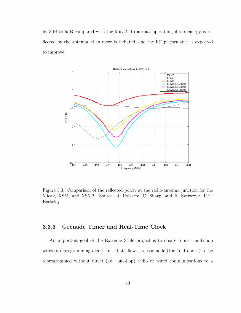
by 3dB to 5dB compared with the Mica2. In normal operation, if less energy is re-

flected by the antenna, then more is radiated, and the RF performance is expected

to improve.

408 413 418 423 428 433 438 443 448 453 458−20

−15

−10

−5

0

5Reflection coefficient of RF path

Frequency (MHz)

S11

(dB

)

Mica2XSMXSM2XSM2, L6=36nHXSM2, L6=39nHXSM2, L6=43nH

Figure 3.3: Comparison of the reflected power at the radio-antenna junction for theMica2, XSM, and XSM2. Source: J. Polastre, C. Sharp, and R. Szewczyk, U.C.Berkeley.

3.3.3 Grenade Timer and Real-Time Clock

An important goal of the Extreme Scale project is to create robust multi-hop

wireless reprogramming algorithms that allow a sensor node (the “old node”) to be

reprogrammed without direct (i.e. one-hop) radio or wired communications to a

43

node which holds a new program image (the “new node”). We argue that robust-

ness consists of two aspects for the case of wireless reprogramming: reliability and

recoverability. Reliabilty refers to the property that all old nodes within direct or in-

direct radio communications with a new node eventually will acquire the new image.

Recoverability refers to the property that regardless of the program image executing

on an old node, the old node will always (eventually) upgrade to the version that a

new node is running. In other words, an incorrect or Byzantine program can never

permanently disable an node from being reprogrammed with a newer image.

A number of algorithms have been proposed for providing over-the-air or multi-hop

wireless reprogramming functionality including the Crossbow In-Network Program-

ming (XNP) [22], Trickle [23], Multi-hop Over-the-Air Programming (MOAP) [24],

and Deluge [25]. All of these algorithms make certain assumptions about their oper-

ation. Chief among these assumptions is that the algorithm itself is actually invoked.

However, as we show in this section, such an assumption cannot be guaranteed on

the existing Mica2 platform and consequently the recoverability property cannot be

guaranteed either.

In a traditional preemptive operating system that runs on hardware support-

ing protected modes of operation, a timer is used to ensure the operating system

maintains control of the processor. Before turning over control of the processor to

application code running in user mode, the operating system sets a timer to interrupt

the processor. When the timer interrupts, control is returned to operating system.

Instructions that modify the operation of the timer are privileged, ensuring that such

instructions can be executed only in protected mode by the operating system [26].

44

The fundamental problem in our case is that like most 8-bit microcontrollers,

the Atmel ATmega128L processor used in the XSM and Mica2 platforms does not

provide a true protected mode of operation. Consequently, it becomes possible for

application code to take nearly complete control over the hardware, disable timers,

turn off interrupts, and leave the operating system with no mechanism to preempt a

misbehaving application. Hijacking of the operating system can occur either acciden-

tally or intentionally. A description of the basic hijacking problem, and one solution

to it, can be found in [27].

At the time of this work, the standard mode of compiling wirelessly reprogrammable

applications under TinyOS is to create a monolithic program image consisting of the

operating system, a wireless reprogramming component, and the user application.

These three components are expected to co-exist in cooperative harmony. There

are many ways to permanently disable wireless reprogramming under this scheme.

Simply downloading an application like “Blink” that does not include the wireless

reprogramming module at all is one way:

/opt/tinyos-1.x/apps/Blink

$ make mica2 install

In this case, the basic ability to wirelessly reprogram is altogether lost. Inserting an

atomic block that never exits works as well:

atomic while (TRUE)

And for the more robust operating system that makes use of the watchdog timer,

the following code will globally disable all interrupts, and loop endlessly, clearing the

watchdog timer. This approach is a slight variation on the previous example:

cli

loop: wdr

jmp loop

45

The problem in the last example is that when interrupts are disabled and the watchdog

timer is cleared periodically, there is no mechanism for the operating system to regain

control. Even if the interrupt vectors are all in a protected code segment, the cli, wdr,

and jmp are fairly common instructions so just their presence in code is not unusual,

especially in interrupt handlers. As a result, it appears non-trivial to “automatically”

detect rogue code. Consider the following “seemingly” normal program that seems

to loop until something happens (but R and b can be chosen such that nothing ever

happens):

cbi R,b

cli

loop: wdr

...

sbis R,b

jmp loop

sei

Atmel has provided a rich set of features making the ATmega128L microcontroller

in-application programmable. Atmel even provides a “quasi-protected” mode of op-

eration that, when enabled through various combinations of fuse settings, makes it

impossible for application code to modify the bootloader or interrupt vectors and

handlers. However, while these features can protect the bootloader and the interrupt

vectors and handlers from the application code, and even the application code from

itself, the features do nothing to guarantee that control eventually returns to trusted

code like the bootloader.

Unfortunately, there is no facility on the ATmega128L to guarantee that execution

eventually returns to trusted code. Furthermore, since it is impractical to hand-

reprogram 10,000 nodes in the event that a misbehaving image is downloaded, we

choose to implement a grenade timer similar to the one described in [27]. A grenade

46

timer is like a watchdog timer which cannot be reset. The most succint description

of the grenade timer is that “once started, the timer cannot be stopped, only sped

up.” The key features of our implementation include:

• Asynchronous Trigger: The grenade timer may be fired by any software at

any time.

• Adjustable Timeout: The amount of time Tfizz that the grenade timer

“fizzes” can be adjusted within bounds, typically by the bootloader, until the

grenade timer’s “pin is pulled.” A software mechanism could exist that allows

application code to request a Tfizz value, within certain bounds, during the next

reset.

• One-Shot Latch-out: Once the grenade timer is started, it cannot be stopped

and Tfizz cannot be changed.

• Alternate Uses: As long as the grenade timer has not been started, the real-

time clock used to implement the grenade timer remains accessible to either the

bootloader or the application and can be used freely.

Our grenade timer circuit is shown in Figure 3.4. The circuit works as follows.

After a power-on-reset (POR), capacitor C60 begins charging through R69 from an

initially discharged state. As long as the voltage across C60 is below VIH , the high-

level input voltage of the AND gate (U39), the output of the AND gate remains low

and the processor remains in reset. The processor’s RD line is automatically tri-stated

during a reset and hence tracks the voltage across capacitor C60. The AND gate’s

other input is pulled high by R57 since the INT output of the DS2417 (U30) is asserted

low only during an interrupt interval and not during a POR.

47

5

5

4

4

3

3

2

2

1

1

D D

C C

B B

A A

ADC1ADC[0..7]

VCC

VCC

VCCVCC

VCC

VCC

SERIAL_ID

WR

RSTN

RD

PWM0

THERM_PWR

Title

Size Document Number R ev

Date: Sheet o f

EXCEPT AS MAY BE OTHERWISE PROVIDED BY CONTRACT, THISDRAWING OR SPECIFICATION IS THE PROPRIETARY PROPERTY OFCROSSBOW TECHNOLOGY INC. IT IS ISSUED IN STRICT CONFIDENCEAND SHALL NOT BE REPRODUCED OR COPIED OR USED (PARTIALLYOR WHOLLY) IN ANY MANNER WITHOUT PRIOR EXPRESS WRITTENAUTHORIZATION OF CROSSBOW TECHNOLOGY INC.

DATEDWN

CHK

APRVD

APRVD 6310-0336-02 A

XSM100CA XTREME SCALE MOTE

Crossbow Technology41 Daggett Drive San Jose, CA. 95134

B2 8Monday, June 14, 2004

X

XX/XX/XX

5-14-04

XX/XX/XX

P. DUTTA

X

M. GRIMMER 5-14-04

POWER/ACCEL/LEDS

remove switch

OHIO STATE UNIVERSITY AND CROSSBOW

U30

DS2417

DIO2

X2 6

INT 3VCC4

X15

C761000pF

SW1

SPDT

12

3

R76100K1%

1

0

U33

NC7SB3157

3

1

65

4

RT1

10K

C16.1uF C60

.1uF

R103

0 OHM

R66

10.0K

Y4

32.768KHZ

21

34

R211K

R20

0 OHM

R70

0 OHM

R64

PHOTO

J6

HDR 2 X 1 X .1

1 1

2 2

R69

10.0K

U20

TC7WH74

D2

CK1Q 5

/Q 3

VCC 8PR7

CL6

R5710.0KR63

4.7K

C15.1uF

U39

74ACH1G08

1

24

5

Figure 3.4: Grenade timer and real-time clock circuit.

The time constant, τ , of the R69C60-circuit is 1ms and the equation for the voltage

across capacitor C60 is:

V (t) = VCC(1− e−t/τ ) (3.1)

Rearranging to solve for t, we have:

t = −τ ln

(1− V (t)

VCC

)(3.2)

At a supply voltage of 3V, the AND gate’s VIH is 2.1V. Substituting 3V and 2.1V

for VCC and V (t), respectively, gives t = 1.2ms. Therefore, after 1.2ms, both of the

AND gate’s inputs are high and the AND gate’s output goes high as well, allowing

the processor to exit the reset state and begin program execution.

The output of the AND gate is also connected to the asynchronous clear input of

the D-type flip-flop U20. By waiting 1.2ms before asserting this line, the power is given

enough time to stabilize before the flip-flop’s state is cleared (set low). Whenever the

flip-flops’s output, Q, is low, the multiplexer/analog SPDT switch (U33), connects

the processor’s SERIAL ID signal to the DS2417’s DIO pin, allowing the processor

48

to communicate with the DS2417, a real-time clock with a built-in timer. To start

the grenade timer, the bootloader loads the value of Tfizz into the DS2417 using the

Dallas 1-wire bus (SERIAL ID) and enables the device. The legal Tfizz values are:

1s, 4s, 32s, 64s, 2048s (34.13min), 4096s (68.27min), 65,536s (18.30hrs), and 131,072s

(36.41hrs).2

The bootloader or application code can start the grenade timer and ensure that

the no subsequent operation can alter or disable the grenade timer, by enabling the

processor’s WR line for output and asserting it high. Doing so creates a low-to-

high transition which has the effect of clocking the positive edge-triggered flip-flop.

Once clocked, the flip-flop output, Q, assumes the value of its input, D. Since D is

tied to VCC , the value of Q goes after the first clock and remains high until it is

asynchronously cleared.

Once Q is high, the multiplexer/analog SPDT switch (U33), disconnects or “latches

out” the processor from communicating with the DS2417. No additional clocking can

reverse this latch-out of the processor until the next DS2417 interrupt occurs or the

processor asserts RD low, both of which asynchronously clears the D flip flop, resets

the processor, and returns control to the bootloader. We note that if neither the

bootloader nor the application code asserts WR high, the DS2417 remains accessible

to the processor and can be used as a real-time clock.

We note that Atmel could have provided nearly equivalent functionality by includ-

ing a fuse setting that disabled non-bootloader control of a timer and its interrupt.

Alternately, Atmel could have provided a non-maskable external interrupt (i.e. an

2These values correspond to the U30’s interval select register IS〈2 : 0〉 values of 000 to 111,respectively. The processor must also enable U30’s oscillator by writing OSC〈1 : 0〉 = 11 and settingthe interrupt enable register, IE, by writing a 1 to this register. After this sequence of operations,the DS2417 will be configured to assert INT low for 122µs every Tfizz seconds.

49

interrupt that cannot be disabled at all). A non-maskable interrupt, when coupled

with the bootloader protection mechanisms and an external source of interrupts, could

have provided a more suitable quasi-protected mode. We do recognize that in certain

embedded applications, all interrupts are legitimately disabled during execution of

the interrupt handler for a variety of quite valid reasons. However, we argue that it

is reasonable to assume that an upper bound exists on the amount of time that any

interrupt handler, or atomic code block, is executing within a critical section. If this

upper bound can be expressed in clock cycles, we envision that a write-once register

could be used to store the maximum amount of time allowed between a non-maskable

interrupt being triggered and either enabling interrupt or execution control being

forcibly transferred to the non-maskable interrupt handler. Perhaps such features,

which can be found in some processors today, will become more common in future

microcontrollers.

The grenade timer can guarantee that the bootloader eventually regains control

of the processor. By properly setting the processor’s fusemap, the bootloader and the

interrupt vectors and handlers can be protected from the application code. However,

we have not yet discussed what the bootloader must do to recognize an outdated (and

perhaps misbehaving) image and recover by either reverting to an earlier image or

downloading a newer image. Those topics will be covered in a later section.

3.3.4 Network Bootloader

Our notion of a network bootloader works in conjuction with the grenade timer to

implement the retaskability and recoverability requirements. The bootloader consists

of a minimal network stack, a network reprogramming module, the grenade timer

50

drivers, and a small application. This bootloader should be factory programmed onto

the XSM and the fuses should be set such that the bootloader can be erased only by

manual reprogramming. The bootloader is responsible for the following operations:

• Version Checking: Check the version of the currently running application

image. The current image’s version number should be stored in an area of

non-volatile memory that is protected from the application code.

• Availability Checking: Check with neighboring nodes for a newer version of

the application image by broadcasting a request and listening for a response.

• Download: Initiate the downloading of a new application image, if any, from

a neighboring node. Keep track of the application image version in boot flash

rather than in the application image or application adjustable memory.

• Integrity Checking: Verify the integrity of a new application image and its

version number through a message authentication code.

• Programming: Move or copy the newly downloaded application image to

make it the default image.

• Arm Grenade Timer: Enable and arm the grenade timer to reset the proces-

sor in time Tfizz.. Disable any further operations on the grenade timer through

the latch-out feature.

• Load Application: Jump to the application entry point and begin execution.

In addition to the responsibilities of the bootloader, the compiler/linker needs to

be configured to relocate the interrupts vectors into a protected region of memory

51

(in particular, the RESET vector) and to generate application images which have a

non-zero entry point.

3.3.5 User Interface

The XSM user interface includes two buttons, three LEDs, a sounder, and a 51-

pin programming port. The RESET button is connected to the processor’s reset line

and depressing this button causes the processor to enter a reset state and releasing

this button allows the processor to begin program execution. The USER button is

connected to a processor interrupt line and requires an interrupt handler to process

the button pushes. Although user applications may modify the availability or func-

tionality of the USER button, the designer’s intent is for this button to serve as a

multi-function input that works in conjuction with the RESET button.

The default configuration of the XSM does not include an ON/OFF power switch.

While this design choice appears to violate generally accepted design principles, we

believe that in this case the choice is warranted. Since the XSM was designed for

use in an experimental network of 10,000 nodes, we wanted to minimize the number

of things which could go wrong including, for example, accidentally deploying nodes

with the power switch set to the OFF position. Another motivation was that we never

imagined that the nodes would be truly turned off in our application. Instead, the

nodes could exhibit various degrees of vigilance ranging from fully awake to deeply

asleep. We did recognize that for research and development purposes, a missing

power switch is just plain annoying. Consequently, we included circuit board pads

and traces so users could populate the power switch after market. The final motivation

for eliminating the power switch was cost.

52

The sounder subsystem includes a transducer capable of producing 98dB in the

4kHz to 5kHz acoustic range. The transducer is driven by an op amp that is pow-

ered from a dual-output charge pump which generates ±2 × VCC . The piezo trans-

ducer’s oscillation frequency is software-controllable but the transducer performs best

at 4.5kHz.

3.4 Sensors

Sensor selection is a fundamental task in the design of a wireless sensor node.

Choosing the right mix of sensors for the application at hand can improve discrim-

inability, reduce density, increase lifetime, simplify deployment, reduce computational

complexity, and lower probability of discovery – in short, improve performance.

Despite the plethora of available sensors, no primitive sensors exist that detect

people, vehicles, or other potential objects of interest. Instead, sensors are used to

detect various features of the targets like thermal or ferro-magnetic signatures. It

can be inferred from the presence of these analogues that, with some probability,

the target phenomenon exists. However, it should be clear that this estimation is an

imperfect process in which multiple unrelated phenomena can cause indistinguishable

sensor outputs. Additionally, all real-world signals are corrupted by noise which

limits a system’s effectiveness. For these reasons, in addition to sensor selection, the

related topics of signal detection, parameter estimation, and pattern recognition are

important [28, 29, 30].

Although several factors contributed to our final choice, the target phenomenolo-

gies (i.e. the perturbations to the environment that our targets are likely to cause)

drove the sensor selection process:

53

• Civilian: A civilian is likely to disrupt the environment thermally, seismically,

acoustically, electrically, chemically, and optically. Human body heat is emitted

as infra red energy omnidirectionally from the source. Human footsteps are im-

pulsive signals that cause ringing at the natural frequencies of the ground. The

resonant oscillations are damped and propagated through the ground. Footsteps

also create impulsive acoustic signals that travel through the air at a different

speed than the seismic effects of footsteps travel through the ground. A person’s

body can be considered a dielectric that causes a change in an ambient electric

field. Humans emit a complex chemical trail that dogs can easily detect and

specialized sensors can detect certain chemical emissions. A person reflects and

absorbs light rays and can be detected using a camera. A person also reflects

and scatters optical, electromagnetic, acoustic, and ultrasonic signals.

• Solder: An armed soldier is likely to have a signature that is a superset of

an unarmed person’s signature. We expect a soldier to carry a gun and other

equipment that contains ferromagnetic materials. As a result, we would expect

a soldier to have a magnetic signature that most civilians would not have. A

soldier’s magnetic signature is due to the disturbance in the ambient (earth’s)

magnetic field caused by the presence of such ferromagnetic material. We might

also expect that a soldier would better reflect and scatter electromagnetic signals

like radar due to the metallic content on his person.

• Vehicle: A vehicle is likely to disrupt the environment thermally, seismically,

acoustically, electrically, magnetically, chemically, and optically. Like humans,

vehicles have a thermal signature consisting of “hotspots” like the engine region

54

and a plume of hot exhaust. Both rolling and tracked vehicles have detectable

seismic and acoustic signatures. Tracked vehicles, in particular, have highly

characteristic mechanical signatures due to the rhythmic clicks and oscillations

of the tracks whereas wheeled vehicles tend to exhibit wideband acoustic energy.

Vehicles contain a considerable metallic mass that affects ambient electric and

magnetic fields more strongly and in an area much larger than a soldier. Vehicles

emit chemicals like carbon monoxide and carbon dioxide as a side effect of

combustion. Vehicles also reflect, scatter, and absorb optical, electromagnetic,

acoustic, and ultrasonic signals.

Of course, there is a tension between the richness of a sensor’s output and the

resources required to process the signals it generates. Imaging and radar sensors, for

example, can provide an immense amount of information but the algorithms needed

to extract this information can have high space, time, or message complexity, making

these sensors unsuitable for use on energy-constrained leaf nodes in a sensor network.

We take that view that a collection of simple sensors, each of which requires low

complexity algorithms for processing, can collaborate as an ensemble to provide a

higher detection signal-to-noise ratio and a lower classification error rate than is

otherwise possible on devices of this class. This view lead us to choose acoustic,

magnetic, and passive infrared as the key components of the XSM sensor suite, with

straightforward target detection and discriminability playing an important role in our

decision.

The strengths of acoustic sensors include long sensing range, high-fidelity, no line-

of-sight requirement, and passive nature. Weaknesses include poorly defined target

55

phenomenologies for certain target classes, high sampling rates for estimation, and

high time and space complexity for signal processing.

The strengths of magnetic sensors include well defined far-field target phenomenolo-

gies, discrimination of ferrous objects, no line-of-sight requirement, and passive na-

ture. Weaknesses include poorly defined near-field target phenomenologies, high con-

tinuous current draw, and limited sensing range.

The strengths of passive infrared sensors include excellent sensitivity, excellent

selectivity, low quiesent current, and passive nature. Weaknesses include line-of-sight

requirement and reduced sensitivity when ambient temperatures are the same as that

of the target.

By fusing simultaneous detections from these sensors, we can discriminate our

target classes using the following classification predicates:

civilian = pir ∧ ¬mag (3.3)

soldier = pir ∧mag (3.4)

vehicle = pir ∧mag ∧mic (3.5)

where pir refers to a passive infrared detection, mag refers to presence of a ferromag-

netic object near a sensor, and mic refers to either wideband acoustic energy or the

presence of harmonics in the acoustic spectra.

3.4.1 Acoustic

The JLI Electronics F6027AP microphone is at the heart of the acoustic subsys-

tem. This sensor is an omnidirectional back electret condenser microphone cartridge.

The microphone sensitivity is −46 ± 2dB (0dB is 1V/Pa at 1kHz), the frequency

56

response is 20Hz to 16kHz. The microphone is cylindrical shaped and 2.5mm tall by

6mm in diameter. This sensor was chosen because of its good sensitivity, small size,

leaded terminals. and overall price/performance.

The output of the microphone is capacitively-coupled and amplified using using

an op amp in an inverting configuration with gain G1 = −91. The output of this gain

stage is again AC-coupled and amplified using an inverting op amp configuration.

The gain of the second stage of amplification is variable using an 8-bit, digitally-

controlled potentiometer. The gain of the second amplifier stage is variable across a

range of G2 = −1.1 to −91, adjustable to one of 256-values along a linear scale (a

logarithmical would have been better). Since these gain stages are cascaded, a total

gain of G1G2 = 100 to 8300, or approximately 40dB to 80dB is possible.

The output of the two gain stages is again capacitively-coupled to eliminate bias

and then low pass filtered. The low pass filter is configured as a single-supply 2-pole

Sallen-Key filter with Butterworth characteristics for minimum passband ripple [31].

The low pass filter circuit is shown in Figure 3.5. The filter transfer function is:

Figure 3.5: Single supply Sallen-Key low pass filter with Butterworth characteristics.

57

H(s) =Vo

Vi

=k

As2 + Bs + 1(3.6)

where k = 1 since we use a unity gain op amp configuration, A = R1R2C1C2 and

B = R1C1 + R2C1 + R1C2(1− k). The filter’s cutoff frequency is:

fc =1

2π√

R1R2C1C2

(3.7)

In our implementation R1 and R2 are each composed of a fixed resistor (1.1kΩ)

in series with a digitally-controlled potentiometer (0 to 100kΩ). The values of R1

and R2 should be set equal for Butterworth characteristics. In our implementation,

C1 = 0.01µF is and C2 = 0.022µF. The ratio of C2/C1 = 2 is used for Butterworth

filter characteristics. The range of cutoff frequencies possible vary from approximately

100Hz when R1 = R2 = 101.1kΩ to 10kHz when R1 = R2 = 1.1kΩ. Resistors R3 and

R4 are 100kΩ resistors which set the signal bias to VCC/2. This biasing is necessary

since the circuit operates from a single supply.

The output of the low pass filter is again capacitively-coupled to eliminate bias

and then high pass filtered. Like the low pass filter, the high pass filter is configured

in a 2-pole Sallen-Key configuration with Butterworth characteristics. The high pass

filter circuit is shown in Figure 3.6. The filter transfer function is:

H(s) =Vo

Vi

=s2kA

As2 + Cs + 1(3.8)

where C = R2C2 + R2C1 + R1C2(1 − k). The coefficients A and k are the same

as in the low pass filter case, and the cutoff frequency is computed in an identical

manner as well. The roles of the resistors and capacitors are reversed in the high pass

filter case so the values of C1 and C2 should be set equal and the ratio R1/R2 = 2

provides Butterworth characteristics. In our implementation R1 and R2 are each

58

Figure 3.6: Single supply Sallen-Key high pass filter with Butterworth characteristics.

composed of a fixed resistor (470Ω and 240Ω, respectively) in series with a digitally-

controlled potentiometer (0 to 100kΩ). The range of cutoff frequencies possible vary

from approximately 20Hz when R1 = 100.47kΩ and R2 = 50.24kΩ to 4.7kHz when

R1 = 470Ω and R2 = 240Ω. Although not shown, the signal bias is set to VCC/2 using

a similar approach as in the low pass filter case. The cascaded filter pair implements

a tunable bandpass filter with independently adjustable cutoffs. Figure 3.7 shows

the frequency response of the low pass filter, high pass filter, and the pair cascaded

together to realize a bandpass filter.

The output of the high pass filter is connected to an ADC channel as well as the

negative input of a comparator. The positive input of the comparator is connected

to the wiper terminal of a digital potentiometer configured as a voltage divider. The

output of the comparator is connected to an interrupt line on the processor. This

circuit allows us to set a detection threshold which, when exceeded, interrupts the

processor, eliminating the need for continuous sampling and signal processing. It it

this wakeup circuit that supports energy-efficient passive vigilance.

59

3.4.2 Magnetic

The Honeywell HMC1052 magnetoresistive sensor is at the core of the magnetic

sensing subsystem. This sensor was chosen because of its two-axis orthogonal sens-

ing, small size, low-voltage operation, low-power consumption, high bandwidth, low

latency, and miniature surface mount package [32]. Internally, the magnetometer is

configured as a Wheatstone bridge whose output is differentially amplified by an in-

strumentation amplifier with a gain G1 = 247. The output of this instrumentation

amplifier is low pass filtered using an RC-circuit with cutoff frequency fc = 19Hz.

The output of the low pass filter is fed into the non-inverting input of a second in-

strumentation amplifier with gain G2 = 78, for a combined gain approaching 20,000

or 86dB. The inverting input of the second instrumentation amplifier is connected to

the wiper terminal of a digital potentiometer configured as a voltage divider. The

instrumentation amplifier’s inverting input is the only user-adjustable parameter in

the magnetometer subsystem and varying it adjusts the bias point of the amplifier.

3.4.3 Passive Infrared

The Kube Electronics C172 pyroelectric sensor is at the core of the passive infrared

subsystem. This sensor consists of two physically separated pyroelectric sensing el-

ements and a JFET amplifier sealed into a standard hermetic metal TO-5 housing

with an integrated optical filter. The sensor is fitted with a compact “cone optics

reflector” that obviates the need for additional lenses. Passive infrared (PIR) sensors

are very popular for detecting human and vehicle presence. These devices are the

central component in many motion sensors for automatic lighting, security systems,

and electric doors. PIR sensors are a good choice for presence and motion detection

60

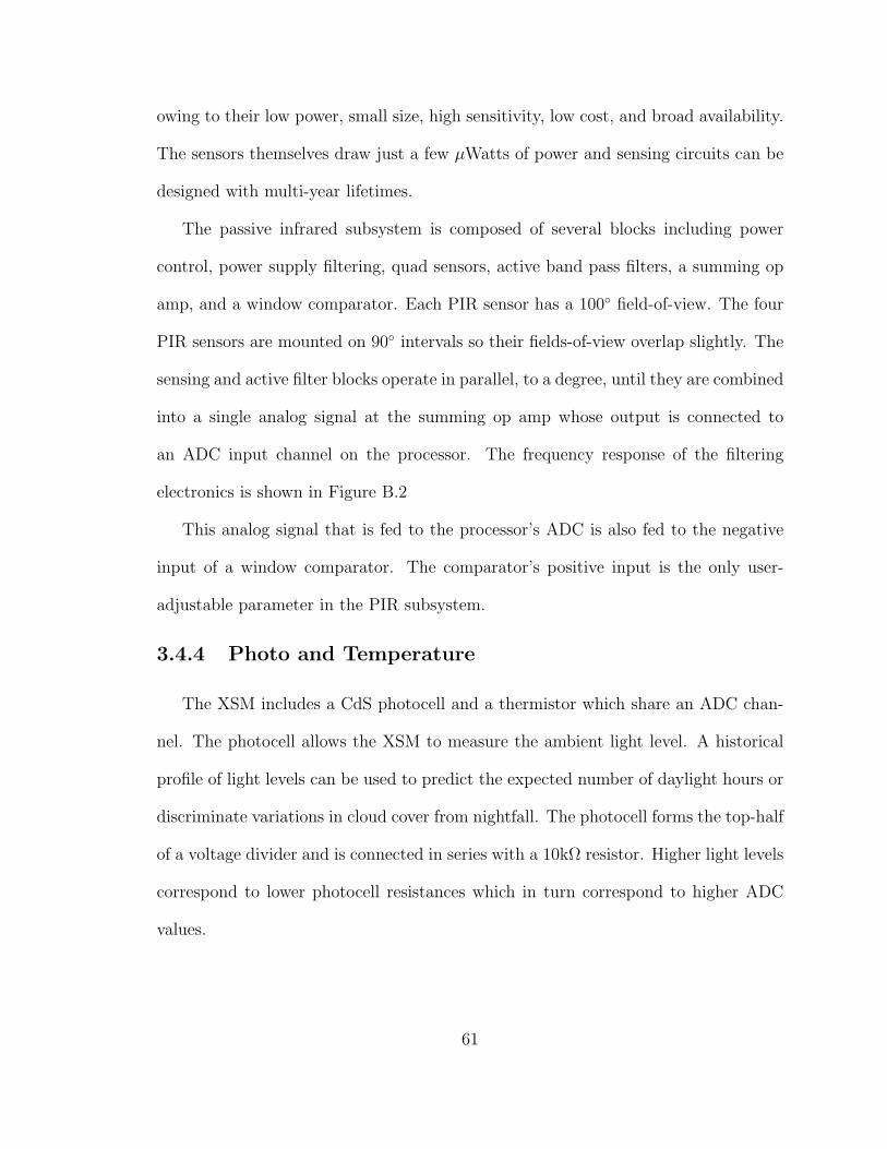
owing to their low power, small size, high sensitivity, low cost, and broad availability.

The sensors themselves draw just a few µWatts of power and sensing circuits can be

designed with multi-year lifetimes.

The passive infrared subsystem is composed of several blocks including power

control, power supply filtering, quad sensors, active band pass filters, a summing op

amp, and a window comparator. Each PIR sensor has a 100 field-of-view. The four

PIR sensors are mounted on 90 intervals so their fields-of-view overlap slightly. The

sensing and active filter blocks operate in parallel, to a degree, until they are combined

into a single analog signal at the summing op amp whose output is connected to

an ADC input channel on the processor. The frequency response of the filtering

electronics is shown in Figure B.2

This analog signal that is fed to the processor’s ADC is also fed to the negative

input of a window comparator. The comparator’s positive input is the only user-

adjustable parameter in the PIR subsystem.

3.4.4 Photo and Temperature

The XSM includes a CdS photocell and a thermistor which share an ADC chan-

nel. The photocell allows the XSM to measure the ambient light level. A historical

profile of light levels can be used to predict the expected number of daylight hours or

discriminate variations in cloud cover from nightfall. The photocell forms the top-half

of a voltage divider and is connected in series with a 10kΩ resistor. Higher light levels

correspond to lower photocell resistances which in turn correspond to higher ADC

values.

61

The thermistor allows the XSM to measure ambient temperature. Such a capabil-

ity has a number of uses. For example, some of the other sensors have temperature

coefficients for parameters like sensitivity and bias point. If the ambient temperature

is known, we can compensate for variations in these parameters. In other cases, a

node may power down in the event that the ambient temperature exceeds the node’s

operating range. Like the photocell, the thermistor forms the top-half of a voltage

divider and is connected in series with the same 10kΩ resistor as the photocell. Care

must be taken to ensure that the operation of the photecell and thermistor is mutu-

ally exclusive. In contrast with the photocell behavior, higher temperatures result in

a higher thermistor resistance, which in turn corresponds to a lower ADC value.

3.4.5 Acceleration

The XSM includes pads and traces for an Analog Devices ADXL202AE accelerom-

eter, and supporting electronics, as shown in Figure 3.9. The ADXL202AE is a small,

low-cost, solid-state, ±2g, dual-axis sensor. We were unable to include this sensor in

the production units due to cost considerations. However, the pads were provided to

gain an additional degree of freedom for our own research and also in the hopes that

future researchers might be able to use this platform to measure acceleration with

some very minor after market modifications.

3.5 Power

The estimated power consumption of the various XSM subsystem is shown in

Table 3.1. The key point to note is that the acoustic and PIR subsystems together

draw 650µA, or approximately 2mW, during continuous operation. This falls within

our acceptable average power budget of 6mW. We note that none of the remaining

62

Subsystem State Current (at 3V) Units

Acoustic off 1 µAAcoustic on 350 µA

Magnetometer off 1 µAMagnetometer on 3 mA

PIR off 1 µAPIR on 300 µA

Sounder off 1 µASounder on 16 mARadio off 1 µARadio receive 8 mARadio transmit 16 mA

Processor sleep 10 µAProcessor active 8 mA

Table 3.1: Estimated current draw of XSM subsystems.

subsystems can be powered continuously without exceeding our power budget. Con-

sequently, we are forced to use a low-power listen mode of communications or perhaps

something more radical like the acoustic sensing channel as a wakeup “radio” since

the XSM includes a sounder capable of producing 98dB of output in the 4kHz to

5kHz frequency range.3 It is also possible that scheduled communications might suf-

fice but it is not obvious that the system latency requirements can be met with such

an approach.

3.6 Packaging

Sensor nodes for intrusion detection may experience diverse and hostile environ-

ments with wind, rain, snow, flood, heat, cold, terrain, and canopy. The sensor

3The wisdom of using such high probability of detect channel in an application for intrusiondetection notwithstanding.

63

packaging is responsible for protecting the delicate electronics from these elements.

In addition, the packaging can affect the sensing and communications processes ei-

ther positively or negatively. Figure 3.10 shows the XSM enclosure and how the

electronics and batteries are mounted. The XSM enclosure is a commercial-off-the-

shelf plastic product that has been modified to suit our needs. Since the enclosure

plastic is constructed from a material that is opaque to infrared, each side has a

cutout for mounting a PIR-transparent window. Similarly, a number of holes on each

side allow acoustic signals to pass through. A water-resistant windscreen mounted

inside the enclosure sensor reduces wind noise and protects the electronics from light

rain. A telescoping antenna is mounted to the circuit board and protrudes through

the top of the enclosure. A rubber plunger makes the RESET and USER buttons

easily accessible yet unexposed.

3.7 Summary

We have presented the requirements, philosophy, and design of the eXtreme Scale

Mote. This is the first highly-integrated mote-class sensor node that directly supports

recoverability and passive vigilance – two essential features for large-scale and long-

lived operation. Recoverability is achieved through the use of a grenade timer. We are

unaware of any other device which implements a hardware grenade timer explicitly

for the purposes of recoverability. Passive vigilance is achieved using wakeup sensing

circuits. These circuits, through the use of low-power sensing and signal conditioning

electronics, combined with an event-driven sensor interface, allow the processor to

sleep a large fraction of the time, extending the system’s lifetime.

64

Figure 3.7: Bode diagram of cascaded Sallen-Key low pass and high pass filters withboth cutoff frequencies set to 4kHz (25krad/sec). The low pass filter magnitude andphase (blue) at 102 rad/sec is 0dB and 0, respectively, and at 106 rad/sec approaches-60dB and -180. The high pass filter magnitude and phase (green) at 102 rad/sec isapproximately -90dB and 180, respectively, and at 106 rad/sec approaches 0dB and0. The cascaded filter response implements a band pass filter that is the sum of thelow pass and high pass filters. The band pass filter magnitude and phase (red) at 102

rad/sec is approximately -90dB and 180, respectively, and at 106 rad/sec approaches-60dB and -180.

65

Date/Time run: 07/03/04 02:31:03PIR Signal Conditioning Circuit Frequency Response

Temperature: 27.0

Date: July 03, 2004 Page 1 Time: 02:31:13

(A) pir_bpf_bode.dat (active)

Frequency

1.0mHz 10mHz 100mHz 1.0Hz 10Hz 100Hz 1.0KHz 10KHzP(V(7))

-400d

-200d

0ddB(V(7)/V(1))

-40

0

40

80

SEL>>

Figure 3.8: Frequency response of PIR signal conditioning circuit for XSM.

5

5

4

4

3

3

2

2

1

1

D D

C C

B B

A A

ADC1ADC[0..7]

PW4

ADC3ADC4

VCC

VCC

VCCVCC

VCC

VCC

VCC

SERIAL_ID

WR

RSTN

RD

PW0

THERM_PWR

I2C_CLK

I2C_DATA

I2C_DATA0

I2C_DATA1

I2C_CLK1

I2C_CLK0

PW [0..7]

ADC[0..7]

Title

Size Document Number R ev

Date: Sheet o f

EXCEPT AS MAY BE OTHERWISE PROVIDED BY CONTRACT, THISDRAWING OR SPECIFICATION IS THE PROPRIETARY PROPERTY OFCROSSBOW TECHNOLOGY INC. IT IS ISSUED IN STRICT CONFIDENCEAND SHALL NOT BE REPRODUCED OR COPIED OR USED (PARTIALLYOR WHOLLY) IN ANY MANNER WITHOUT PRIOR EXPRESS WRITTENAUTHORIZATION OF CROSSBOW TECHNOLOGY INC.

DATEDWN

CHK

APRVD

APRVD 6310-0336-02 A

XSM100CA XTREME SCALE MOTE

Crossbow Technology41 Daggett Drive San Jose, CA. 95134

B2 8W ednesday, June 30, 2004

X

XX/XX/XX

5-14-04

XX/XX/XX

P. DUTTA

X

M. GRIMMER 5-14-04

POWER/GRENADE TIMER/LEDS

remove switch

OHIO STATE UNIVERSITY AND CROSSBOW

U30

DS2417

DIO2

X2 6

INT 3VCC4

X15

C761000pF

R113

330K

C17.1uF

SW1

SPDT

12

3

R76100K1%

R103

0 OHM

U8

ADXL202AE

ST1

T22

GND3

YOUT 4XOUT 5

YFILT 6XFILT 7

VCC8

R112

100

1

0

U33

NC7SB3157

3

1

65

4

RT1

10K

C16.1uF C60

.1uF

R110

4.7KC18.1uF

R108

4.7K

Y4

32.768KHZ

21

34

R66

10.0K

R211K

R70

0 OHM

R111

4.7K

J6

HDR 2 X 1 X .1

1 1

2 2

R64

PHOTO

R109

4.7K

U20

TC7WH74

D2

CK1Q 5

/Q 3

VCC 8PR7

CL6

R69

10.0K

C19.1uF

R5710.0K

C15.1uF

R634.7K

R107

4.7K

U39

74ACH1G08

1

24

5

R200 OHM

R22

4.7K

Figure 3.9: Accelerometer circuit available on the XSM (unpopulated).

66

Figure 3.10: This model shows how the XSM electronics and batteries are mountedin the enclosure. Source: Crossbow Technology.

67

CHAPTER 4

DETECTION AND CLASSIFICATION OFFERROMAGNETIC TARGETS

Most targets of military interest contain ferromagnetic materials which perturb

the ambient magnetic field surrounding the object. Soldiers carry guns, bullets, and

grenades. Vehicles have considerable ferrous content in the wheels, engines, and un-

dercarriage. These targets exhibit characteristic signatures. By detecting changes in

the ambient magnetic field, it is possible to detect the presence of these and other

target classes. In addition, by extracting parameters of the space-time varying mag-

netic fields surrounding these targets, we can can discriminate between certain tar-

get subclasses. In this work, we consider detection and classification techniques for

discriminating soldiers from vehicles using the space-time signatures of these target

classes. We also demonstrate techniques for energy-efficient use of sensors.

Deeply embedded and densely distributed networked systems that can sense and

control the environment, perform local computations, and communicate the results

will allow us to interact with the physical world on space and time scales previously

imagined only in science fiction. This enabling nature of sensor actuator networks has

contributed to a groundswell of research on both the system issues encountered when

building such networks and on the fielding of new classes of applications [33, 34, 12].

68

Perhaps equally important is that the enabling nature of sensor networks provides

novel approaches to existing problems, as we illustrate in this work in the context of

a well-known surveillance problem.

4.1 Related Work

Detection and classification of targets is a basic surveillance or military applica-

tion, and has hence received a considerable amount of attention in the literature.

Recent developments in the miniaturization of sensing, computing, and communica-

tions technology have made it possible to use a plurality of sensors within a single

device or sensor network node. Their low cost makes it feasible to deploy them in

significant numbers across large areas and consequently, these devices have become a

promising candidate for addressing the distributed detection and classification prob-

lems. A variety of approaches have been proposed that range over a rich design space

from purely centralized to purely distributed, high message complexity to high com-

putational complexity, data fusion-based to decision fusion-based, etc. The spatial

density and redundancy that is possible due to the diminishing cost of a single node

favors highly distributed models. The constraints of network reliability and load per-

mit sending only a limited amount of data over the network, and in some extreme

cases, even a single bit of data. Such binary networks have been used in previous

work for tracking [35, 36, 37]. Even classification schemes based on low dimensional

decision fusion [38] require significant local signal processing.

In contrast to our work, much of the work on target classification in sensor net-

works has used a centralized approach. This typically involves pattern recognition

or matching using time-frequency signatures produced by different types of targets.

69

Caruso, et. al. [39] describe a purely centralized vehicle classification system using

magnetometers based on matching magnetic signatures produced by different types of

vehicles. However, this and other such approaches require significant a priori config-

uration and control over the environment. In [39], for instance, the vehicle has to be

driven directly over the sensor for accurate classification and at random orientations

and distances, the system can only detect presence. Such an approach also imposes

high computational burden on individual nodes. Meesookho, et. al. [40], describe

a collaborative classification scheme based on exchanging local feature vectors. The

accuracy of this scheme, however, improves only as the number of collaborating sen-

sors increases, which imposes a high load on the network. By way of contrast, Duarte

et. al. [38] describes a classifier in which each sensor extracts feature vectors based

on its own readings and passes them through a local pattern classifier. The sensor

then transmits only the decision of the local classifier and an associated probability of

accuracy to a central node that fuses all such received decisions. This scheme, while

promising since it only slightly loads the network, requires significant computational

resources at each node.

4.2 Target Model

In this section, we present our model of both soldiers and vehicles as a magnetic

dipoles. A moving soldier or vehicle, or more generally, a moving ferromagnetic object

can be modeled as a moving magnetic dipole centered at (x, y, z). Still more generally,

the dipole position can be described as a function of time if x, y, and z are replaced

with x(t), y(t), and z(t), respectively.

70

The dipole is modeled as two equal but opposite equivalent magnetic charges +q

and −q, separated by a distance l = 2r, where r is the radial distance from the dipole

center to a charge. The orientation of the dipole is given in spherical coordinates

relative to the dipole center. The zenith (polar) angle φ and the azimuthal angle

θ, together with r, fully specify the position and orientation of the magnetic dipole,

as illustrated in Figure 4.1. As before, a more general description of the dipole’s

orientation as a function of time can be given by replacing the angles φ and θ with

time dependent versions φ(t) and θ(t) or position dependent versions φ(x, y, z) and

θ(x, y, z).

A non-uniform ferromagnetic object like a vehicle will have a more complex mag-

netic signature composed of dipoles of varying strengths and moment arm lengths

representing the engine block, axles, spare tires, roof, and other parts. These finer-

granularity components can be modeled in an additive manner due to superposition

effects. However, for a first order analysis sufficient for vehicle detection, a single

dipole provides an adequate estimate of the magnetic flux density B at the origin

B =µ

4πq

(r1

r31

− r2

r32

)(4.1)

where

r1 = (x + r sin θ cos φ)x + (y + r sin θ sin φ)y + (z + r cos θ)z (4.2)

and

r2 = (x− r sin θ cos φ)x + (y − r sin θ sin φ)y + (z − r cos θ)z (4.3)

The magnetic flux density B is composed of the following components:

B = Bxx + Byy + Bzz (4.4)

71

r

x

z

y

x

z

y

r

r 1

r 2

Figure 4.1: Magnetic dipole model.

where Bx, By, and Bz are the rectangular components given by:

Bx =µ

4πq

[x

(1

r31

− 1

r32

)+ r sin θ cos φ

(1

r31

+1

r32

)](4.5)

By =µ

4πq

[y

(1

r31

− 1

r32

)+ r sin θ cos φ

(1

r31

+1

r32

)](4.6)

Bz =µ

4πq

[z

(1

r31

− 1

r32

)+ r cos θ

(1

r31

+1

r32

)](4.7)

and where r1 and r2 are the magnitudes of r1 and r2, respectively:

r1 =√

(x + r sin θ cos φ)2 + (y + r sin θ sin φ)2 + (z + r cos θ)2 (4.8)

72

and

r2 =√

(x− r sin θ cos φ)2 + (y − r sin θ sin φ)2 + (z − r cos θ)2 (4.9)

4.3 Sensor Platform

Our sensor platform consists of the Mica2 processor/radio board and the Mica

Sensor Board, both available from Crossbow Technology.

4.3.1 Mica2 Processor and Radio Board

The familiar Mica2 mote, a derivative of the Mica family of motes developed at

U.C. Berkeley [41], served as our network node. The Mica2 offers an Atmel AT-

mega128L processor with 4KB of RAM, 128KB of FLASH program memory, and

512KB of EEPROM memory for logging. The motes run the TinyOS operating sys-

tem [42], and are programmed using the NesC language [43].

4.3.2 Mica Sensor Board

Our sensor node includes the popular Mica Sensor Board. This board includes

a 2-axis magnetometer, 2-axis accelerometer, microphone, thermistor, photosensor,

and sounder. For this work, we only used the magnetometer subsystem on the Mica

Sensor Board. The core of this circuit is the Honeywell HMC1002 dual 4-element

magnetoresistive wheatstone bridge. The HMC1002 can detect magnetic fields as low

as 30 µgauss and up to ±6 gauss (earth’s magnetic field is 0.5 gauss). The nomi-

nal sensitivity of the magnetometer is 1.0mV/V/gauss, which means the differential

output fluctuates 1.0mV per volt of supply voltage per gauss of magnetic field.

Some historical context might also be useful. The first use of magnetometers on

the Mote platform can be traced back to COTS Dust in 2000 [44]. While a design

73

for a magnetic field sensor, based on the NVE AA002-02 magnetic field sensor, is

presented, no fundamental motivating application is apparent.

Shortly thereafter, in March 2001, researchers demonstrated a fixed/mobile ex-

periment for tracking vehicles with a UAV-delivered sensor network at Twentynine

Palms [45]. While the sensorboard used in that experiment, called the “Magnetome-

ter Board,” never became available commercially, its design, based on the Honeywell

HMC1002 magnetometer [32], did become available [46] and served as the basis for

several future magnetometer designs.

The Mica Sensor Board owes part of it heritage to the Twentynine Palms sen-

sorboard and is in broad use across the sensor networking research community. Our

motivation for using the Micasb was to leverage a standard sensorboard platform. The

Honeywell magnetometer experiences both drift and a decrease in sensitivity when

exposed to temperature swings or strong magnetic fields. The Honeywell sensor in-

cludes a set/reset input to reduce this drift and resensitize the magnetometer using a

high current pulse. Unfortunately, the Mica Sensor Board lacks of any circuitry that

implements this set/reset feature.

4.4 Towards Low-power Sensing

A major concern with the magnetometer circuit present on the Mica Sensor Board

is its power consumption of nearly 20mW during continuous operation. Approxi-

mately 90% of the power is consumed by the sensor itself and the remaining power is

consumed by the signal conditioning electronics.4 One popular approach to lowering

4We note that the Mica Sensor Board design uses a pair of instrumentation amplifiers for eachmagnetometer channel. These amplifiers draw 175µA each and could be replaced with low-poweroperational amplifiers that draw less than 25µA each.

74

the power consumption of sensor circuits is to duty-cycle the sensor and supporting

electronics. The magnetometer is a predominantly resistive element with a bandwidth

of 5MHz and nanosecond-scale latencies, so it is well suited to duty-cycled operation.

However, the signal conditioning circuit is not suited to duty-cycled operation because

of the phase delay of a low pass filter used for anti-aliasing and 60Hz noise reduction

[47].

An analog low pass filter needs a continuous-time input so just duty-cycling the

magnetometer would result in a chain of low pass filter step responses as the power

to the sensor is toggled on and off. To compensate, we might turn on the sensor,

wait the settling time, and then take a sample. Since this filter has a time constant

τ = RC = 20kΩ×1µF=20ms, the settling time of the filter to a step response is about

5τ or 100ms, so duty-cycling will help reduce power consumption only at sampling

rates lower than 10Hz. Eliminating the filter altogether will cause aliasing and is

generally considered poor design for ADC circuits.

To address the problem of a low startup-latency, high-power sensor coupled with

a high-latency, low-power signal conditioning circuit, we propose the use of a mixed-

signal, multi-phase clocked, sample-and-hold control circuit as the interface between

the sensor and signal conditioning electronics. This approach is not limited to the

magnetometer and can be used for any sensor that satifies the low startup-latency

requirement. Our sample-and-hold control circuit is shown in Figure 4.2.

This circuit works as follows. Whenever VCC is applied to the SHC POWER

line, schmitt triggers U1 through U4 are turned on. Schmitt triggers U1 and U2 are

part of an oscillator circuit whose duty cycle and frequency is set using capacitor C1

and resistors R2 and R3. For a small (unbalanced) duty cycle, DC, in which the

75

5

5

4

4

3

3

2

2

1

1

D D

C C

B B

A A

ADC6

MAG_PWR

MAG_PWR

MAG_VREF

MAG_HOLD

MAG_PWR

MAG_VREF

MAG_PWR

I2C_CLK

MAG_PWR

MAG_PWR

ADC5

MAG_HOLD

MAG_PWR

I2C_DATA

MAG_PWR

MAG_PWR

MAG_VREF

PW5

HOLD

MAG_SENSOR_PWR

SENSOR_PWR

SHC_PWR

VCC

VCC

I2C_DATA1

MAG_SR

I2C_CLK1

PW[0..7]

ADC[0..7]

Title

Size Document Number R ev

Date: Sheet o f

EXCEPT AS MAY BE OTHERWISE PROVIDED BY CONTRACT, THISDRAWING OR SPECIFICATION IS THE PROPRIETARY PROPERTY OFCROSSBOW TECHNOLOGY INC. IT IS ISSUED IN STRICT CONFIDENCEAND SHALL NOT BE REPRODUCED OR COPIED OR USED (PARTIALLYOR WHOLLY) IN ANY MANNER WITHOUT PRIOR EXPRESS WRITTENAUTHORIZATION OF CROSSBOW TECHNOLOGY INC.

DATEDWN

CHK

APRVD

APRVD 6310-0336-02 A

XSM100CA XTREME SCALE MOTE

Crossbow Technology41 Daggett Drive San Jose, CA. 95134

B7 8Fr iday, A ugust 13, 2004

X

XX/XX/XX

5-14-04

XX/XX/XX

P. DUTTA

X

M. GRIMMER 5-14-04

OHIO STATE UNIVERSITY AND CROSSBOW

MAGNETOMETER SENSOR

ADDR[00]

R51

330

C581.0uF

U15

HMC1052

GNDB1

OUTB+2 GNDA1 3

OUTA+ 4

VB

R5

SR+6

OUTB-7

SR-8

GNDA2 9

OUTA- 10

V+

V-

+

-

U?LMC7215

5

31

2

4

U17A

AD5242

A1 2

W1 3

B1 4

SD6SCL7SDA8

AD09

AD110

O1 1

C561.0uF

C?0.1uF

U?

MAX4597

IN1

COM2

GND

3

NC 4

VCC

5

C551.0uF

U68F

74HC14A/SO

13 12

C?0.1uF

U3

5 6

C2

R55

25.5K

R7

C521.0uF

R2

R43

100K

C53

0.1uF25V

D1

GAIN

SNSVREF

U13B

INA2126

15

16

13 14

1110

12

U?

MAX4597

IN1

COM2

GND

3

NC 4

VCC

5

U1

1 2

14

7

U16

TLE2426

OUT 1

GND2IN3

NC4

NC5 NC 6NC 7NR 8

GAIN

V+

V-

SNSVREF

U18A

INA2126

2

1

4 3

98

67

5

R52

1.10K

R49

25.5K

U14

IRF7507

SN1GN2SP3GP4 DP 5

DP 6

DN 7

DN 8

R44

8.25K

U4

9 8

R6

R3

U17B

AD5242

A2 16

W2 15

B2 14

O2 13VSS12

VCC5

GND11

R41

200

V+

V-

+

-

U?LMC7215

5

31

2

4

R47

25.5K

R53

25.5K

C571.0uF

C1

C541.0uF

R50

8.25K

R5

Q3

ZXM61P03F

1

32

U68E

74HC14A/SO

11 10

U2

3 4

GAIN

V+

V-

SNSVREF

U13A

INA2126

2

1

4 3

98

67

5

C6510uF

R45

330

GAIN

SNSVREF

U18B

INA2126

15

16

13 14

1110

12

C3

R42

10.0K

R46

1.10K

Figure 4.2: Sample-and-hold control circuit.

Ton/(Ton + Toff ) << 1, R2 is chosen to be much smaller than R3 so that when D1

is forward-biased, R2 and R3 are both in C1’s path but when D1 is reverse-biased,

only R3 is in C1’s path. The output of the oscillator is used to enable (power on)

and disable (power off) the sensor. The SENSOR PWR signal powers on the sensor

during the Ton time and turns off the sensor during the Toff time. The sensor transient

time, Tt, is the amount of time required for the sensor output to stabilize (also known

as the sensor’s startup latency).

This SENSOR PWR signal is also connected to a positive edge detector formed

from capacitor C2, resistor R5, and schmitt trigger U3. Assume C2 is in a discharged

state and SENSOR PWR is low. Then, U3’s input will be low and output will be

76

high. If SENSOR PWR transitions from low to high, as would occur when the oscil-

lator output changes from Toff to Ton, this low-to-high transition passes through the

capacitor and causes the output of U3 to go low. C2 begins to charge through R5,

which causes the voltage across R5 to decrease until C2 is fully charged. When the

voltage across R5 reaches VIL, the low-level input of U3, the output of U3 transitions

from a low state to a high state. The purpose of this edge detector is create a delay

after the SENSOR PWR low to high edge. This length of this delay must exceed the

startup latency of the sensor.

The output of the first positive edge detector is connected to a second positive

edge detector formed from capacitor C3, resistor R6, and schmitt trigger U4. The

output of this second edge detector is normally high but it generates a negative pulse

(high to low to high) when the detector detects a positive edge on its input. The

output pulse of the edge detector provides the HOLD signal and is connected to the

control line of an analog switch (not shown). When the HOLD signal is low, the hold

capacitor tracks (samples) the output voltage of the sensor. When the HOLD signal

is high, the hold capacitor is disconnected from the sensor and holds the last tracked

output value of the sensor.

The width of the edge detector’s output pulse is chosen to exceed the turn on

time of the analog switch that connects the sensor to hold capacitor and the charging

time of the hold capacitor (not shown). Note that the second of the edge detectors

is triggered on the rising edge of the preceding positive edge detector output. Recall

that at the time of the positive edge detector’s rising edge, the output of the sensor

has stabilized so the sampling period occurs during a stable sensor signal. Note that

77

the oscillator’s on time Ton must exceed the sum of the width of the pulses that are

generated from the two edge detectors.

The time constant, τ = RC, of a positive edge detector determines the width

of the high to low to high pulse that is generated when the edge detector’s input

transitions from low to high. When the capacitor, C, is charging after a low to high

transition on the input, the voltage across the resistor, R is:

V (t) = VCC(1− e−t/τ ) (4.10)

Substituting VIL for V (t) and rearranging to solve for t, we have:

t = −τ ln(1− VIL

VCC

)(4.11)

The output of the hold capacitor, buffered with an op amp, is connected to the

remaining signal conditioning electronics just like the sensor would be in the absence

of the sample-and-hold control circuit.

The current consumption of the sample-and-hold control is less than 50µA and

the current consumption of the additional op amps is similar, for an increase of nearly

100µA. This increase is overshadowed by the significant decrease in average current

consumption owing to the duty-cycling of the sensor itself. With low latency sensors,

duty cycles of 1% or less are easily achievable.

4.5 Detection

The component graph of the detection signal chain for ferromagnetic targets is

shown in Figure 4.3. The modules of this signal chain include a limiter, low pass

filter (noise filtering), decimator, moving statistics, constant false alarm rate (CFAR)

78

Figure 4.3: Magnetometer signal detection chain.

detector, low pass filter (hysteresis), and energy estimator. The outputs of the de-

tector include signal duration and signal energy content. Addition modules could

include a peak estimator or a hidden markov model for finer-grained signature anal-

ysis supporting classification. This signal chain operates independently on each of

the two magnetometer axes and fuses the readings together at each node. Such local

fusing reduces false alarms caused by spurious noise along only one axis. The design

philosophy of the signal detection subsystem is that all operations occur in response

to events – that is, the arrival of new data samples or timer events drives signal

processing. Sampling occurs with a certain predetermined frequency, fs, which is a

function of Vmax and the noise power spectral density. In the future, we envision an

adaptive sampler that adjusts to varying noise power and frequency.

A detailed description of the signal chain modules include:

79

• Limiter: The limiter is a non-linear module that acts to limit the samples that

are large in magnitude in an effort by the detector to reduce the effect of noise

outliers. Without the limiter, the PD could be reduced substantially.

• Low Pass Filter: The FIR low pass filter computes a moving average of the

signal to reduce noise and improve the PFA.

• Decimator: The decimator allows downsampling to rates more appropriate for

our signal phenomenology.

• Moving Statistics: The moving statistics module estimates the signal mean

and variance over the previous n data samples every time a new sample becomes

available.

• CFAR Detector: The output of the CFAR detector is true during the interval

in which a target passes by the sensor and false otherwise. This module esti-

mates the signal duration. The module implements a Neyman-Pearson detector

that works by building a histogram, which serves as a proxy for the probability

density function, of the signal variance in the noise over a long period of time

and then compares it to the (nearly) instantaneous signal variance as reported

by the moving statistics.

• Hysteresis: The hysteresis is implemented using an IIR low pass filter over

the signal variance. The IIR filter provides a “fast-attack, slow-decay” response

(i.e. a non-constant phase shift). Such a response was desired in order to

avoid breaking up a single detection event into multiple smaller detections.

80

The downside, however, is that stronger signals cause longer decay times and

biases the duration estimation non-linearly before it is reported.

• Energy Estimator: The energy estimator module determines the energy con-

tent of the signal of interest. The estimator begins computing the energy con-

tent of the signal when the output of the signal detector is true and stops when

the output of the signal detector is false. The interval over which the energy

content is computed is the duration of the signal. The energy is computed by

subtracting the moving average, or bias, from the signal and then summing the

squares of the samples over the period of the signal. An event is signaled upon

completion of the energy content computation.

• Classifier: The classifier fuses the various parameters (duration, energy, etc.)

and, optionally, can attempt to categorize the target into one of several classes.

4.6 Classification

The goal of ferromagnetic classification is to correctly label a target as belonging

to one of several classes including soldier and vehicle. Vehicles contain significantly

greater amounts of metallic mass than soldiers and consequently vehicles magnetically

affect much larger areas than soldiers do. In general, each ferromagnetic target class

has a minimum and maximum area in which it disrupts earth’s ambient magnetic

field in a manner that is detectable by our sensors. In this section, we formalize the

notion of this area, called the target’s “influence field,” develop an estimator for it,

and analyze the estimator’s performance for varying degrees of network reliability

and latency.

81

4.6.1 The Influence Field as a Spatial Statistic

The influence field is the size of the area in which a target can be detected. In

practice, the influence field is the union of the areas bounded by the curves of equipo-

tential field strength where the signal-to-noise ratio exceeds the sensor’s minimum

detectable threshold. Since the size and shape of this area changes as a function of

sensor calibration and sensitivity, noise power, and other nuisance parameters like

target orientation, the area is bounded by a maximum and minimum value and is

best treated as a random variable We will show that a Gaussian approximation is a

suitable model for the random variable. The influence fields of different target classes

are usually different, both in relative and absolute terms, from one sensing mode to

the next. A vehicle may have a 5× larger magnetic influence field than a person but

a 50× larger acoustic influence field than the same person.

The following example will serve to further illustrate this concept. Assume that

nodes are deployed with a density of λ and that the nominal area of the influence field

is A. Then, the number of sensors, n, that can simultaneously detect the object is

given by n = Aλ, or more generally by the range [Aminλ, Amaxλ]. If target classes do

not have overlapping influence field ranges, then the system can discriminate between

target classes by examining the value of n. For example, assume a regular grid on

5-foot centers giving a deployment density of λ = 1/52 = 0.04 sensors/sqft, and a

target with a minimum and maximum influence radius of 12 ft and 15 ft, respectively.

Then, Amin = π122 = 452 sqft and Amax = π152 = 707 sqft. We find that between

nmin = Aminλ = 0.04 × 452 = 18 and nmax = Amaxλ = 0.04 × 707 = 28 sensors will

detect the target’s presence at a single point in time. Given the same deployment

density, assume a second target with a minimum and maximum influence radius of 5

82

ft and 8 ft, respectively. Then, Amin = π52 = 79 sqft and Amax = π82 = 201 sqft. We

find that between nmin = Aminλ = 0.04×79 = 3 and nmax = Amaxλ = 0.04×201 = 8

sensors will detect the second target’s presence at a single point in time.

For practical reasons, we associate with the influence field a window of time in

which the target is detected. There are several factors that influence the choice of the

size of this window. The number of nodes that can detect a moving target in a given

interval of time may depend upon the size of the object, the amount of ferromagnetic

content and hence the range at which it can be detected by a magnetometer, the

velocity of the target, and the number of sensors in the region around the target.

Therefore, we must consider the density of node deployment and the size and speed

of the target types.

Based on target motion models for our target classes, we identify the smallest

and the slowest moving ones as well as the largest and fastest moving ones. The

amount of time required to process the data for a given window must be less than

the window duration in order to meet the needs of a real-time online system. We are

also concerned with the concurrent detection of the same event at different sensors

because of differences in the hardware, the sensitivity of sensors, or the parameters

of the detection algorithm running at the sensor node. For instance, a fast-attack,

slow-decay detector, like the one used in our signal detection software, can affect sen-

sors in a non-linear and non-deterministic manner, causing perceived time differences

between the starts and ends of detections at different nodes for the same event. This

uncertainty in detection duration, which can be as large as 500ms, also affects the size

of the influence field window. Finally, we also have to factor in the effect of network

unreliability on the number of messages corresponding to the detection events that

83

are actually received at the classifier. Based on these factors, we selected 500ms as the

width of the influence field window. In an ideal case, we would we have sensors with

constant phase delay, a window size of zero, and deterministic network performance.

Given classification’s required window size, we must verify that detection events

occurring at the same physical time are timestamped accordingly with values that

be converted to the same relative timebase at the classifier. In order to achieve this

common timebase, we propose using ETA, the Elapsed Time on Arrival protocol. This

service also needs to guarantee that the maximum difference in the estimates of any

two nodes in the network does not exceed some fraction of the classifier window size.

For instance, for a window size of 500 ms and a classification accuracy of exceeding

99%, we require that the accuracy of the time synchronization service to be within

1% of 500ms or 5ms.

4.6.2 Influence Field Estimator

In order to estimate the influence field, each node that detects a target transmits

a single bit representing the target’s presence along with the elapsed timestamp of the

presence detection and a monotonically increasing event identifier. Once again, upon

detecting the target’s absence, the node transmits the elapsed timestamp with the

same event identifier (each presence-absence pair shares an event identifier). These

presence and absence messages are convergecast to the classifier service running on

a distinguished node, which in our case is the base station located at the root of the

network. The duration of the target’s presence in a particular node’s field of view

is easily computed by taking the difference in the timestamp values from the pair

messages sharing an event id received from that node.

84

4.6.3 Classifier Design

The classifier collects data received from the network and partitions it into win-

dows of global time. Once the incoming data has been partitioned into windows

based on global time, the classifier counts the number of nodes that have detected

the presence of an target in that window. To conserve the network bandwidth, nodes

simply report the start and the end of a detection event. Hence, the classifier has

to maintain a history of nodes that have started detecting an event but have not yet

stopped detecting it. The classifier carries forward the count of such active nodes

from one window to the next. Further, all detection events in a classification window

need not belong to the same target. For instance, if multiple targets simultaneously

in the network, each target will be detected by the nodes in the region surrounding it.

The classifier distinguishes multiple targets and does not combine these simultaneous

detections into a single larger target.

Wind and other sources of noise can cause nodes to report false detections. The

classifier identifies such outliers that could skew the classification. Consequently,

the classifier uses localization information about the reporting nodes and knowledge

of the target motion and phenomenological models. For example, if the classifier

receives only two detection events and the influence field for the smallest target type,

the soldier, is expected to be between 4 and 9 for the given density considering

50% network reliability, the classifier identifies these nodes as outliers and does not

generate a classification. If, on the other hand, the influence field for a soldier is

9 while that for a car is 36, and if 4 soldiers walk through the network at the same

time such that they are at sufficient distance from one another, the classifier identifies

that the corresponding events belong to different targets and accurately classifies the

85

targets as 4 soldiers rather than a single car. Note that the data association problem is

automatically addressed because of the fine-grained spatial locality of the detections.

The output of the classifier at the end of each classification window is one or more

classification decisions along with the supporting evidence, in the form of a set or sets

of nodes, that are associated with the given target.

Classifier latency is an important tunable parameter that governs the length of

time that the classifier waits between receiving the first detection event and providing

the first classification result. The classifier masks detection events until it has received

a sufficient number of samples to achieve the desired probability of false alarm, PFA.

In addition, the classifier introduces a delay while waiting for enough samples to

report a meaningful classification. Consequently, the classifier latency is only one of

two components that contribute to the overall system latency. The other component

of system latency is the latency between detecting a target at the sensor node and

reporting that detection to the classifier. We investigate the classifier performance as

a function of latency in the next section.

4.6.4 Validation

A theoretical model of a target’s influence field, parameterized with the target’s

size, speed, heading, inclination, location, and ferro-magnetic content can be used to

demonstrate that the probability density functions of the various target classes are

discriminable. However, an accurate model of a target’s influence field may be difficult

to achieve without incorporating many nuisance parameters and even still may require

time consuming finite element methods to compute. Due to the spatial, temporal, and

class-conditional variations of the numerous nuisance parameters, we present a simple

86

lumped parameter model of the computed strength and shape of the influence field for

both a soldier and a vehicle in Figure 4.4. The soldier is modeled as carrying a gun of

length 3 ft at an azimuthal angle of 20. The vehicle is modeled as the superposition

of the influence fields of the engine, front axle, rear axle, transmission, spare tire, and

steering wheel. In both cases, the positive y-axis is pointing toward the northwest and

the field strength displayed is the planar projection of the magnetic field at ground

level across the displayed area. These models should convey a sense of the relative

shape of the influence fields and an intuitive understanding of their discriminability.5

Since we do not know the true weights and variations of the parameters, we will use

empirical methods to validate the model.

Figure 4.4: The shape of the influence field of a soldier and a vehicle.

5Note: the field strength is not scaled the same for both plots. Hence, these plots demonstratethe shape but not the relative size of the influence fields.

87

As with any real system, experimental validation of performance is necessary. In

the case of the influence field as an estimator of the target’s class, this validation

exists at three levels: the theoretical influence field, the influence field as measured

by the sensor nodes, and the influence field as reported to the classfier. Due to

the complexity of the theoretical model, the remainder of this section will focus on

empirical measurements of the influence field at the sensor nodes and its estimate

at the classifer. The key distinction is that the estimated influence field is a noisy

function of the measured influence field, network reliability, latency, probability of

detection and false alarm, detector hysteresis, and nuisance parameters described

earlier. How much “noise” is added and in what quantities as a result of these

additional parameters in reality is not clear. Consequently, we vary a few easily

controllable parameters such as speed, heading, network reliability and latency, and

lump the remaining parameters.

Figure 4.5 shows the influence field probability distributions for a soldier and a

car, as actually measured by the sensors. The measured influence field of a soldier

has a mean, µ, of 12.2 and a variance, σ2, of 0.44 while a car has a mean of 43.5

and a variance of 0.49. We overlay on this figure a pair of curves ∼ N (12.1, 1)

and ∼ N (43.5, 1.5), approximating the influence field of a soldier and a vehicle,

respectively. It should be clear from Figure 4.5, that there exists a clear separation

between the measured influence fields for a soldier and a car. Since the distributions

have nearly identical variances, we can compute the discriminability, d′, as

d′ =|µ2 − µ1|

σ= 67 (4.12)

which indicates a practically infinitesmal probability of mis-classification.

88

0 10 20 30 40 500

0.05

0.1

0.15

0.2

0.25

0.3

0.35

0.4Measured Influence Field

Number of Detecting Nodes, N

P(ω

i|N)

Soldier (ω1)

Vehicle (ω2)

0 10 20 30 40 500

0.05

0.1

0.15

0.2

0.25

0.3

0.35

0.4Approximated Influence Field

Number of Detecting Nodes, N

P(ω

i|N)

Soldier (ω1)

Vehicle (ω2)

Figure 4.5: The influence field of a soldier and a car as measured at the sensor nodes,and their Gaussian approximations.

We note that these influence field values are ideal in the sense that they are based

on data obtained directly at the nodes and not necessarily the data that is actually

available to the classifier. In order to evaluate system performance, we study the

effects of network unreliability and latency on the classifier performance by varying

the transmission power level (3, 6, 9, and 12), the number of transmissions per message

(1, 2, 3, 4, 5), and the classifier latency (5, 10, and 15 seconds). In all, we run a total of

280 experiments using 16 different parameter configurations (a subset of the possible

parameter space). Analyzing the timestamped measurements at the nodes and at the

classifier, we identify in Figure 4.6 the parameter values which best demonstrate the

variability in the estimator performance as a function of reliability and latency. We

use the notation MAC(P,T,L), where P is the power setting, T is the total number

of transmissions, and L is the latency in seconds.

89

0 10 20 300

0.1

0.2

0.3

0.4MAC (9,1,5)

0 10 20 300

0.1

0.2

0.3

0.4MAC (9,1,10)

Pro

babi

lity

0 10 20 300

0.1

0.2

0.3

0.4MAC (9,1,15)

Estimated Influence Field

0 10 20 300

0.1

0.2

0.3

0.4MAC (9,3,5)

VehicleSoldier

0 10 20 300

0.1

0.2

0.3

0.4MAC (9,3,10)

Pro

babi

lity

0 10 20 300

0.1

0.2

0.3

0.4MAC (9,3,15)

Estimated Influence Field

Figure 4.6: Probability distribution of the estimated influence field as a function ofmedia access control (MAC) power, transmissions, and latency. MAC(P,T,L), whereP is the power setting, T is the total number of transmissions, and L is the latencyin seconds.

The confusion matrix for MAC(9,1,5) is shown in Table 4.1. The classifier perfor-

mance is clearly unacceptable with this optimistic single transmission per node and

a classifier latency of 5 seconds.

We find that increasing the latency to 10 seconds, as shown in MAC(9,1,10),

improves the classifier performance to 100%. Recall, however, that we used a lumped

parameter approach that did not attempt to characterize the influence field over the

90

Soldier Vehicle

Soldier PCS,S= 31% PCS,V

= 69%Vehicle PCV,S

< 1% PCV,V> 99%

Table 4.1: The confusion matrix for the influence field classifier for MAC(9,1,5) as-suming the PCV,V

> 99% requirement is met.

entire range of all possible parameters. Consequently, the probability distributions of

the influence fields would likely have greater variance than our test cases indicate and

would likely overlap, reducing the discriminability to an unacceptable level. Since

increasing the latency from 5 to 10 seconds improves the classifier performance, we

are motivated to further increase latency, to 15 seconds, as shown in MAC(9,1,15).

We find, however, that no further improvement in discriminability results from this

increase in latency. We still remain interested in improving the classifier performance,

so we must consider other parameters.

Turning our attention to reliability, we attempt to transmit each message at most

three times (i.e. two retransmissions) and with a latency of 5 seconds. The results

are shown in MAC(9,3,5). We find that our attempt to increase network reliability

has actually decreased the discriminability of the target classes since the probability

distributions now overlap even more so than with MAC(9,1,5). We attribute this poor

performance to the increased traffic generated from retransmissions and its attendant

effects on collision and congestion. Next, we try MAC(9,3,10) and notice an improve-

ment over MAC(9,3,5) in that the discriminability has improved. We also note the

MAC(9,3,10) results in a distribution whose variance is smaller than MAC(9,1,10).

91

Encouraged by the positive trends in both separating the means and decreasing the

variances, we investigate MAC(9,3,15) and find that it offers the best discriminability.

We notice that while MAC(9,3,15) offers the best overall performance, the worst

case network reliability is approximately 50%, since only one-half of the detections at

the nodes are actually available to the classifier. We also note that the network loss

rate varies according to target class. There is less variation in the soldier’s influence

field than in the vehicle’s, as estimated at the classifier across all of our tests. The

soldier’s estimated influence field ranges from 9 in MAC(9,1,5) to 6.4 in MAC(9,3,5),

a decrease of 27% and 48%, respectively, from the measured value of 12.2. In con-

trast, the vehicle’s estimated influence field ranges from 21.2 in MAC(9,3,15) to 7.7

in MAC(9,3,5), a decrease of 51% and 82%, respectively, from the measured value of

43.5. In other words, the network delivers approximately twice the reliability for a

soldier than it does for a vehicle. We attribute this wide variation to the different

levels of traffic that are generated isochronously for the different target classes. As-

suming a 10% margin of error in the influence field estimation and greater than 99%

classification accuracy, we find that the acceptable lower bound on network reliability

for classification is approximately 50%.

We have focused our attention on discriminating soldiers from vehicles. We now

turn to sensor fusion in order to address the classification of persons, and to make our

detection of soldiers and vehicles more robust. Recall that the radar motion sensors

detect all of the target classes but only the ferro-magnetic targets are detected by

the magnetic sensors. Consequently, we can fuse these two sensing modalities into a

single predicate that the classifier evaluates at the end of each window to determine

whether a person, and only a person, is present

92

We also use sensor fusion to make the detection of soldiers and vehicles more

robust

soldier = magnetic ∧ (f < x∗) (4.13)

vehicle = magnetic ∧ (f ≥ x∗) (4.14)

where f is the estimated influence field and x∗ is the decision boundary that minimizes

the classification error rate. In our case, x∗ = 14.

93

CHAPTER 5

TOWARDS UWB RADAR-ENABLED SENSORNETWORKS

Ultrawideband (UWB) radar-enabled sensor networks have the potential to ad-

dress key sensing, classification, tracking, and localization challenges common to many

intrusion detection applications. We investigate the suitability of UWB radar as a

sensing technology for resource-constrained sensor networks. We consider sensor-

specific factors like range, power, latency, interference, and size. In addition, we also

consider low space, time, and message complexity algorithms for signal detection,

parameter estimation, and target classification. Our work is grounded in off-the-

shelf sensor and processor hardware along with some custom supporting electronics.

Preliminary laboratory experiments and field trials demonstrate promising results al-

though much work remains before the sensors can be deployed in unknown or hostile

environments.

5.1 Introduction

Traditionally, intrusion detection systems have used infrared, acoustics, seismic,

and magnetics for passive sensing, and optics and ultrasonics for active sensing,

94

but radar has been conspicuously absent. Conventional radio detection and rang-

ing (radar) systems employ transmitted and reflected microwaves to detect, locate,

and track objects over long distances and large areas. Due to its versatility, radar has

found applications in defense, law enforcement, meteorology, and mapping. However,

widespread commercial applications of radar have been limited because conventional

systems are expensive, bulky, and difficult to use.

A new kind of radar sensor system based on time domain reflectometry (TDR)

techniques and ultrawideband (UWB) technology was developed in the mid-1990s at

Lawrence Livermore National Labs [48]. Livermore’s tradename for its version of the

sensor is micropower impulse radar or MIR. Livermore’s MIR sensors are inexpensive,

compact, and low-power – while still offering detection, ranging, and velocimetry

capability – which makes them ideal for use with wireless sensor networks. MIR,

like conventional radar, uses transmitted and reflected microwaves. However, unlike

conventional systems that transmit bursts of narrowband continuous waves, MIR

uses very short, and consequently ultrawideband, pulses and is therefore also called

ultrawideband radar or just UWB radar. These short pulses contain very little energy

but since the energy they do contain is spread across a broad range of frequencies,

UWB signals are better able to penetrate obstacles and are more immune to multipath

effects. UWB radar technology has been used for proximity detectors, motion sensors,

rangefinders, electronic dipsticks, graphics tablets, stud finders, and tripwires. For

the remainder of this work, we will use the term “UWB radar” or simply “radar”

when referring to ultrawideband radar sensors which operate on this principle.

As an active rather than passive technology, UWB radar has a larger sensing

radius than either infrared or magnetic sensors and consequently UWB radar can

95

be deployed in lower densities. UWB radar sensors require neither line-of-sight like

infrared sensors nor exposure to the environment like acoustic sensors, making them

easy to conceal inside of trees, rocks, or other objects which are impervious to light

and sound. For foot traffic, UWB and seismic sensors offer similar sensing range

but unlike seismic sensors, UWB radars do not need to be staked into the ground.

UWB radars are active sensors since they transmit short bursts of RF energy but

since their transmissions are very short, the pulses usually appear to be background

noise. The sensors can be made both difficult to detect and resistant to jamming by

dithering the pulse repetition rate or using other coding techniques. In addition to

these benefits, UWB radar-enabled sensor nodes can determine an object’s range and

speed, and in some cases, estimate an object’s size. It is for these and other reasons

that radar-enabled sensor networks promise a new level of performance in wide-area

intrusion detection systems.

5.2 Theory of Operation

Ultrawideband radar is available in two broad categories: pulse Doppler and pulse

echo. Pulse Doppler radar operates on the Doppler principle and is primarily used

for motion sensing. Pulse echo radar employs time-of-flight and is typically used as

a rangefinder. For this work, we use pulse Doppler radar sensors. Consequently, for

the remainder of this work, when we refer to UWB radar, we mean pulse Doppler

radar unless explicitly stated otherwise.

UWB radar works by transmitting a short pulse and listening for its reflection.

If the object that reflects the transmitted pulse is moving, then the frequency of the

reflected pulse will be Doppler-shifted to a frequency that is slightly different from the

96

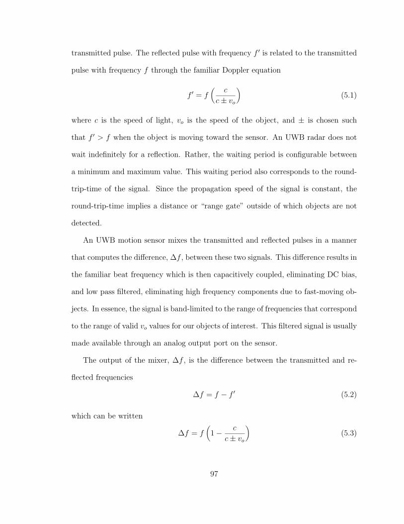
transmitted pulse. The reflected pulse with frequency f ′ is related to the transmitted

pulse with frequency f through the familiar Doppler equation

f ′ = f(

c

c± vo

)(5.1)

where c is the speed of light, vo is the speed of the object, and ± is chosen such

that f ′ > f when the object is moving toward the sensor. An UWB radar does not

wait indefinitely for a reflection. Rather, the waiting period is configurable between

a minimum and maximum value. This waiting period also corresponds to the round-

trip-time of the signal. Since the propagation speed of the signal is constant, the

round-trip-time implies a distance or “range gate” outside of which objects are not

detected.

An UWB motion sensor mixes the transmitted and reflected pulses in a manner

that computes the difference, ∆f , between these two signals. This difference results in

the familiar beat frequency which is then capacitively coupled, eliminating DC bias,

and low pass filtered, eliminating high frequency components due to fast-moving ob-

jects. In essence, the signal is band-limited to the range of frequencies that correspond

to the range of valid vo values for our objects of interest. This filtered signal is usually

made available through an analog output port on the sensor.

The output of the mixer, ∆f , is the difference between the transmitted and re-

flected frequencies

∆f = f − f ′ (5.2)

which can be written

∆f = f(1− c

c± vo

)(5.3)

97

rearranging to solve for vo and simplifying

vo = ±c

(∆f

f −∆f

)(5.4)

Since we know c and f , if we can estimate ∆f , then we can also determine vo.

For example, if a UWB radar with a 2.4GHz center frequency outputs a signal with

∆f =16Hz, an object would be moving with a radial velocity of 2m/s.

We can further simplify the computation by recognizing that for the objects of

interest to us, ∆f << f , so

vo = ±c

(∆f

f −∆f

)(5.5)

becomes

vo ≈ ±c

(∆f

f

)(5.6)

and a signal’s wavelenth λ = c/f gives

vo ≈ ±∆fλ (5.7)

and a signal’s period ∆T = 1/∆f gives

vo ≈ ±λ/∆T (5.8)

A sinusoidal signal encounters a zero-crossing every ∆Tz = ∆T/2, which corresponds

to half of a wavelength. Estimating ∆Tz is a matter measuring the elapsed time

between successive zero crossings.

In addition to the target object, the transmitted pulse is reflected or “scattered”

by other nearby objects like rocks, trees, and walls which are of no interest. We

refer to these useless reflections as clutter. The strength of a reflection is a function

of an object’s shape, size, permittivity εr, and permeability µr. Fortunately, most

98

of the objects that cause clutter are stationary and their reflections, no matter how

strong, are filtered out. Therefore, in theory, the beat frequency due to clutter is

zero and the sensor’s analog output is a constant voltage. However, in practice, we

find that some background noise (e.g. due to environmental effects or thermal noise)

and clutter noise (e.g. due to a leaf fluttering in the wind) do have an effect on

the sensor’s output. Some of this noise is also filtered out but some of it is not.

Distinguishing between noise and a signal of interest due to a legitimate object is the

topic of detection.

5.3 Sensor Platform

Our sensor platform consists of several circuit boards including a processor/radio

board, an ultrawideband radar motion sensor, and a generic sensor board. While

these devices are available off-the-shelf, no off-the-shelf products were found which

were suitable for the interface circuitry or the packaging, so custom electronics and

enclosures were used. Figure 5.1 shows the stack of circuit boards used to implement

our sensor network node.

5.3.1 Radar Sensor and Antenna

We used the TWR-ISM-002 sensor shown in Figure 5.2 and available from Ad-

vantaca [49] as our radar sensor platform. This sensor detects motion up to a 60ft

radius around the sensor but this range is adjustable to a shorter distance using an

onboard potentiometer. The sensor includes a 51-pin connector designed to interface

mechanically with the expansion connector on the Mica Motes [41]. The sensor re-

quires 3.4V - 6.0V (nominally 3.6V) and draws less than 1mA from this supply. The

99

Figure 5.1: Radar sensor network node electronics. The circuit boards from top tobottom are: (i) dipole antenna for transceiving the radar signal, (ii) radar sensor,(iii) interface/power board, (iv) generic sensor board, and (v) processor/radio board.The battery case which holds two AA batteries can be seen at the bottom of the stack.

unit also requires a precise power source to provide 5.5V with a ±1% tolerance and

draws a nominal 7.5mA from this second supply.

The sensor provides a fast-attack and slow-decay digital output meaning that the

output is asserted immediately after detecting a target but is not unasserted until

approximately one second after the target is no longer detected. The sensitivity, like

the range, can be adjusted using a potentiometer. Adjusting the sensitivity simply

varies the detection threshold used for the digital output. We found the sensor’s

digital output had a high false alarm rate outdoors even though indoors, the digital

output performed quite well.

In addition to the digital output, an analog output is available. The analog

output is a lowpass-filtered version of the Doppler baseband signal. The lowpass filter

response has a 3 dB/octave drop-off above 18 Hz and an additional 12 dB/octave

above 220 Hz. The analog output signal varies from 0V to 2.5V and is nominally

biased at 1.25V when there is no motion. When a target is moving within sensing

100

range and with a radial velocity component, the analog output oscillates between 0V

and 2.5V. The output is a noisy, potentially clipped, weighted sum of sinusoids whose

frequencies are related to the radial velocity of each reflecting surface (e.g. chest,

arms, legs, etc.) and whose amplitude is related to the strength of the reflection.

Since our application required robust detection outdoors, we used the analog output

and digitally processed the signals using the detection and estimation algorithms

presented in this work.

Figure 5.2: Advantaca TWR-ISM-002 pulse Doppler ultrawideband radar motionsensor.

The sensor includes a dipole antenna board which mounts on top of the radar

sensor board using an MMCX connector. A null in the antenna plane makes it

possible for a target moving along a radial in this plane to go undetected.

5.3.2 Mica Power Board

Despite the mechanical compatibility through the expansion connector interface,

matching signal pin assignments, and common power pin assignments between the

radar sensor and the Mica mote, the radar does require different and incompatible

101

operating voltages. The Mica motes require, and through the expansion connector

provide, the raw battery voltage which can vary from 3.3V nominally to 2.7V or lower.

Since the supply voltages required by the radar sensor board exceed the voltages

and tolerances provided by the our batteries, we designed a circuit consisting of a

pair of boost switching regulators to generate these higher voltages and provide the

necessary tolerances. The Mica Power Board implements this circuit and is shown in

Figure 5.3. The board owes its odd footprint with a U-shaped cutout in the upper

left and a square with rounded corners in the middle to a desire to maintain physical

compatibility with the existing Mica Sensor Board.

Figure 5.3: The Mica Power Board has two fully independent switching regulatorsthat are potentiometer adjustable and can deliver 3V - 40V at 200mA each.

The Mica Power Board has two fully independent switching regulators that are

potentiometer adjustable and can deliver 3V - 40V at 200mA each. The circuit

works by intercepting the two power signals available through the bottom expansion

connector and replacing these signals with the outputs of the two regulators and then

passing the regulator output through the top connector. The Mica Power Board also

102

includes a shutdown feature. When the board is in the shutdown state, power is

simply passed though the board as if it were not present.

5.3.3 Mica Sensor Board

Our sensor node includes the popular Mica Sensor Board. This board includes a

2-axis magnetometer, 2-axis accelerometer, microphone, thermistor, photosensor, and

sounder. We had planned on using the magnetometer but discovered that the mere

presence of the radar interfered with the magnetometer readings. We conducted a

variety of experiments to isolate the source of the interference but in the final analysis,

we were unable to pinpoint the source of the interference.

5.3.4 Mica2 Processor and Radio Board

The familiar Mica2 mote, a derivative of the Mica family of motes developed at

U.C. Berkeley [41], served as our network node. The Mica2 offers an Atmel AT-

mega128L processor with 4KB of RAM, 128KB of FLASH program memory, and

512KB of EEPROM memory for logging. The motes run the TinyOS operating sys-

tem [42], and are programmed using the NesC language [43].

5.3.5 Packaging

Sensor nodes for intrusion detection may experience diverse and hostile environ-

ments with wind, rain, snow, flood, heat, cold, terrain, and canopy. The sensor

packaging is responsible for protecting the delicate electronics from these elements.

In addition, the packaging can affect the sensing and communications processes either

positively or negatively.

103

Our enclosure is smooth and capsule shaped, as shown in Figure 5.4. This shape

provides a self-righting capability and minimizes wind-resistance. The enclosure body

is clear to allow sunlight to illuminate a solar cell mounted inside. Unfortunately, this

has the side effect of heating the electronics to a level at which they intermittently

fail. The sensor electronics are mounted on a frame that attached to the enclosure

shell using a single gimbal mechanism. The gimbal is free to rotate along the long

axis of the enclosure. The frame is asymmetrically weighted in favor of the side

with batteries so that the batteries are on the bottom and a solar cell is on top.

The gimbal mechanism, when coupled with the rotational degree of freedom of the

cylindrical enclosure, increases the likelihood that the radar and radio antennas plane

will be perpendicular to the ground and the solar cell will be pointing toward the sky,

helping to increase the node’s sensing range, communications range, and lifetime.

5.4 Power Considerations

A major concern with the radar circuit used in this work is its power consumption

of nearly 45mW during continuous operation. Unfortunately, this sensor also has a

high-latency initialization process, as can be seen in Figure 5.5.

As a result of this high-latency initialization process, we find this particular sensor

a poor fit as a low-power wakeup sensor. This is not a fundamental limitation of the

technology, however, and we are aware of other radar systems with an “instant on”

capability.

104

Figure 5.4: Self-righting enclosure used for packaging the radar sensor.

5.5 Detection

From a signal processing perspective, detection refers to the process of determin-

ing when a signal of interest is present. To bridge the notion of detecting an object’s

presence with the notion of detecting a signal’s presence, we must have a model

that relates the two. The model should also describe how the sensor will respond to

background noise and clutter noise. The analog output of pulse Doppler radar will os-

cillate about a bias point with frequency components that are principally determined

by speed of moving clutter and moving objects, when present, as well as background

noise. The analog output’s amplitude is determined by the size, shape, permittivity,

and permeability of moving clutter and objects.

105

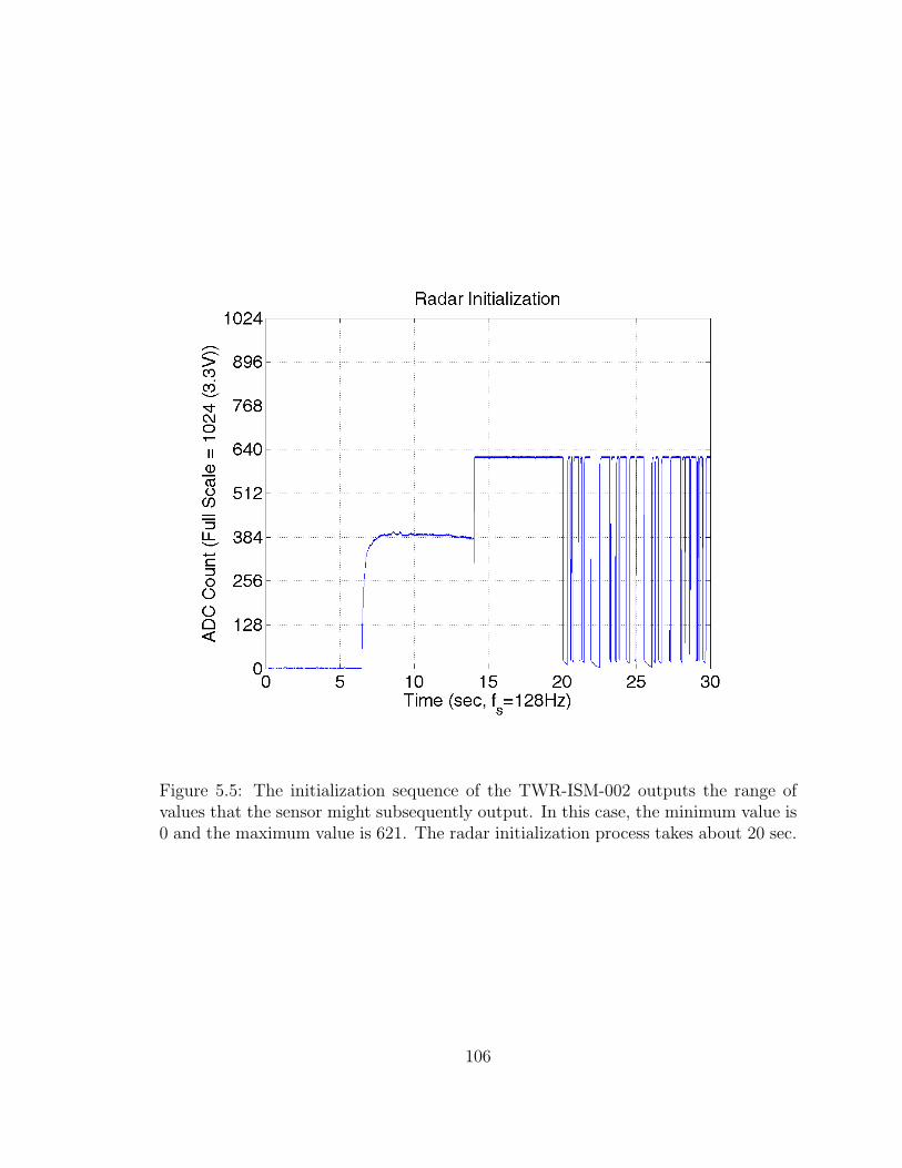
Figure 5.5: The initialization sequence of the TWR-ISM-002 outputs the range ofvalues that the sensor might subsequently output. In this case, the minimum value is0 and the maximum value is 621. The radar initialization process takes about 20 sec.

106

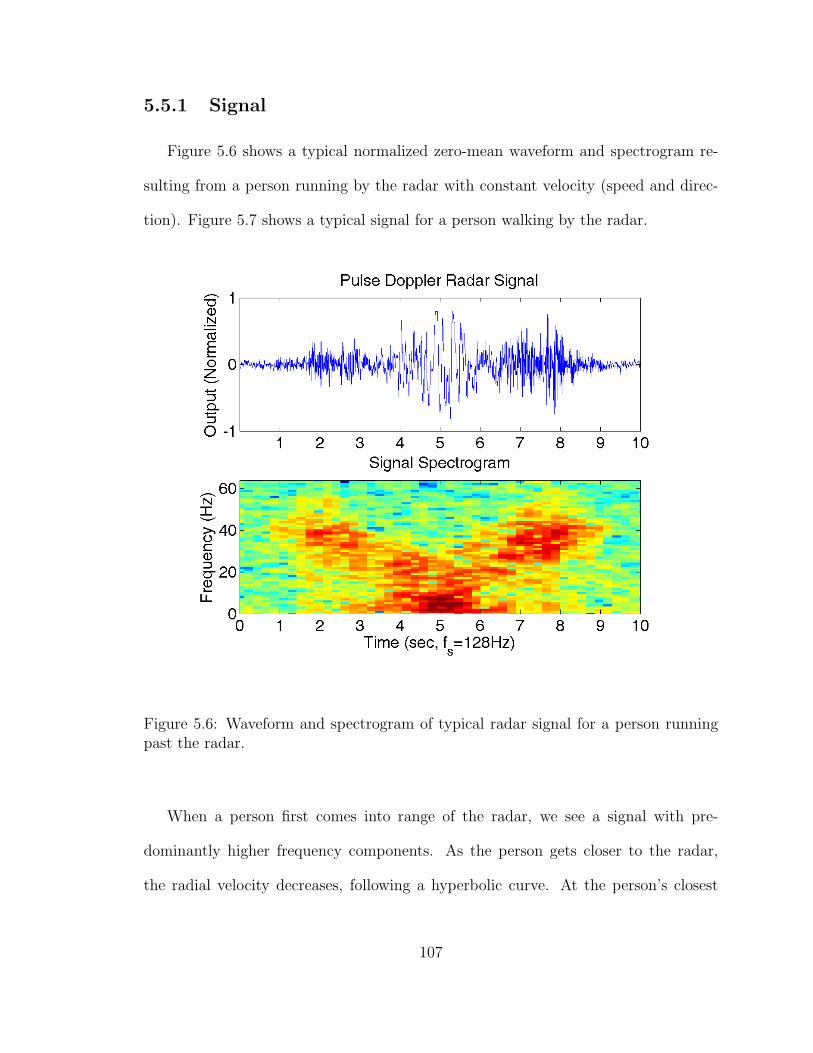
5.5.1 Signal

Figure 5.6 shows a typical normalized zero-mean waveform and spectrogram re-

sulting from a person running by the radar with constant velocity (speed and direc-

tion). Figure 5.7 shows a typical signal for a person walking by the radar.

Figure 5.6: Waveform and spectrogram of typical radar signal for a person runningpast the radar.

When a person first comes into range of the radar, we see a signal with pre-

dominantly higher frequency components. As the person gets closer to the radar,

the radial velocity decreases, following a hyperbolic curve. At the person’s closest

107

Figure 5.7: Waveform and spectrogram of typical radar signal for a person walkingpast radar.

108

point-of-approach (CPA) to the radar, the radial velocity approaches zero, assum-

ing a non-zero CPA. At this point, lower frequency components dominate the power

spectrum. Then, as the person moves away from the sensor, essentially the mirror

image of the first half of the waveform is repeated. Figures 5.8, 5.9, and 5.10 show

additional radar waveforms.

Figure 5.8: Sample signal data for person walking past sensor. The red line is theestimated bias, computed as the mean of the data set.

109

Figure 5.9: Sample signal data for person running past sensor. The red line is theestimated bias, computed as the mean of the data set.

110

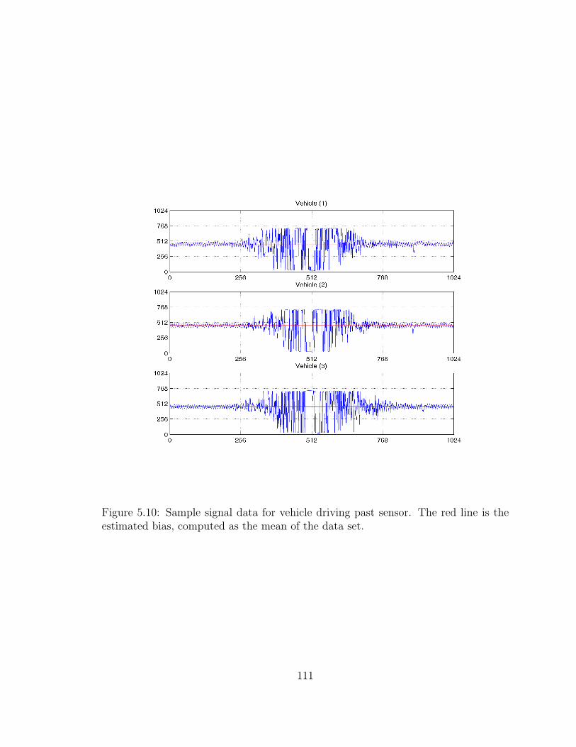
Figure 5.10: Sample signal data for vehicle driving past sensor. The red line is theestimated bias, computed as the mean of the data set.

111

5.5.2 Noise and Clutter

Background noise tends to be normally distributed and wide sense stationary over

time constants larger than the time constant of a typical passing object. However,

background noise may not be wide sense stationary over much larger timescales due,

for example, to solar or meteorological effects. Similary, we note that there are

occasions in which the noise is not independent and identically distributed. That

is, we find the occasional presence correlated of noise. This is particularly true for

clutter noise due to a fluttering leaf, a flying bird, or heavy rainfall, for example,

and is more difficult to discriminate from signals caused by the motion of legitimate

targets of interest. Figure 5.11 shows the observed noise at several different times

and locations.

In the time domain, which is what we are practically limited to on processors

of this class, the main differences between clutter and objects of interest are that

clutter sometimes has a lower energy content (i.e. the signal amplitude is smaller)

and frequently tends to be more bursty (i.e. lasts for a shorter period of time than

legitimate targets) but occasionally tends to far less bursty (i.e. lasts for a longer

period of time than a legitimate target).

5.5.3 Energy Detector

Initially, we used a binary-hypothesis energy detector to discriminate between

noise (H0) and a signal of interest (H1). After subtracting the bias from the radar’s

analog output, the signal is averaged over a moving window of size N and squared to

compute the energy, E. The window size N is chosen to be small enough so that the

detector is agile and large enough that the detector is stable in the presence of noise.

112

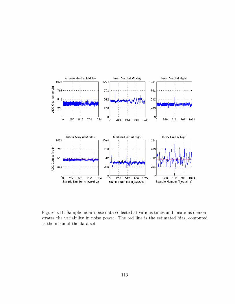
Figure 5.11: Sample radar noise data collected at various times and locations demon-strates the variability in noise power. The red line is the estimated bias, computedas the mean of the data set.

113

Determining the bias point requires care since over short intervals, the signal is

often skewed. One way to address this issue is to use a longer window when computing

the bias. In our implementation, the average bias x is determined over the trailing

Nk samples of the raw signal. In order to conserve memory, this computation is

performed hierarchically and with a block scheme modulo N , resulting in a space

complexity of kN . The value of Nk is chosen such that it reflects the time constant

of the environment and is empirically determined by application of the Central Limit

Theorem until filtered background noise has Gaussian statistics.

Variations in individual sensors or battery levels can also affect the signal statistics

across different sensors or on the same sensor over time. In our case, the UWB radar

sensors are powered from a DC boost regulator which maintains a constant output

voltage even when the input battery voltage sags. However, there is no such boost

regulator for the processor or its ADC voltage reference. As a result, when the battery

voltage sags, the both the bias point and signal of the UWB radar sensor appear to

increase. While it is possible to compensate for battery droop using the internal

bandgap reference in the processor, such an approach is not sufficient since there are

still other effects that affect the bias point.

A similar approach is used to determine the average energy E of the background

noise over a similarly long time interval. Since even the background noise varies over

large timescales, a constant false alarm rate (CFAR) detector is used to provide an

adaptive decision threshold, γ, for the energy detector. The detector decides

H =

H0 if E ≤ γH1 if E > γ

where γ is computed

γ = ασE + E (5.9)

114

where the value of α is the one that satisfies

PFA = 1−∫ α

−∞

1√2π

e−12x2

dx (5.10)

for a required false alarm rate, PFA.

Unfortunately, the CFAR energy detector is not immune to clutter noise like

fluttering leaves or heavy rain. The types of correlated noise and clutter shown in

Figure 5.11 is quite prevalent in our waveforms and hence must be dealt with in our

detection algorithms to achieve acceptable false alarm rates. Traditionally, discrimi-

nating such clutter from legitimate objects requires additional signal processing but

we will consider another method.

5.5.4 Histogram-similarity Detector

A simple CFAR energy detector will fail in the presence of highly-correlated noise

or clutter. It may be possible to reduce the false alarm effects of correlated noise by

averaging the signal over a longer window or by estimating additional parameters of

the signal, but this approach requires greater memory and processing. An alternate

detector design that better discriminates clutter from a legitimate object, without

increasing algorithmic complexity, is desirable.

Due to the issues with a simple energy detector, we implemented a different detec-

tion algorithm based on histogram matching. The motivation behind this approach

is due to the discernable probability distribution functions (PDF) of signal, clutter,

and noise. Our observation is that it is simpler to directly correlate the prototype

PDFs with the observed PDFs and select the prototype class with which the observed

samples has the strongest correlation.

115

The details of our approach are as follow. The sensor output is normalized and

quantized. The output of the quantizer is histogrammed over a moving window.

The quantization level, window size, and window overlap are all adjustable. The

bins in each histogram window are converted to elements in a test vector which is

then compared with a set of prototype vectors. The hypothesis corresponding to the

prototype which has the highest correlation to the test vector is selected.

Figure 5.12 shows a moving histogram of the radar signal amplitude as a result

of ambient background noise and heavy rain. Figure 5.13 shows a moving histogram

of the radar signal amplitude as a result of a person walking by and a car driving

by. Notice the conspicuously dense clusters near the top and bottom bins for the

car and person, but the absence of a dense cluster near the top and bottom bins in

the cases of background noise and heavy rain. Conversely, notice the conspicuous

absence of high density clustered near the middle bins for the car and person, but

the presence of high density near the middle bins in the cases of background noise

and heavy rain. By finding the greatest correlation between a sampled histogram and

a set of pre-collected prototype histograms or priors, the detector can discriminate

many types of clutter from objects of interest. Our approach essentially compares

the probability densities of the sampled data and prototypes directly.

Normalization and Quantization

A feature of the TWR-ISM-002 sensor is that within the first 30 seconds or so after

being powered up, the sensor enters an initialization phase during which it outputs

a signal that spans the entire range of values the sensor might subsequently output

during normal operation, as shown in Figure 5.5.

116

Figure 5.12: Signal amplitude (raw) and moving histogram (normalized) of radaroutput due to background noise and heavy rain taken over a 32 second period with asampling rate of 128Hz and a histogram window, bins, and overlap of 256, 0, and 16,respectively.

We monitor the output of the sensor during this time and store the minimum and

maximum amplitude values, Amin and Amax, respectively, that are observed. These

values are then used to precompute a mapping function between the sensor output and

the normalized and quantized values used for histogramming. The mapping function

uses a binary search and can map an input value onto an output value with only

O(lgN) comparisons, where N is the number of quantization levels. In contrast, if

computational resources were not at a premium, a normalize and quantize operation

117

Figure 5.13: Signal amplitude (raw) and moving histogram (normalized) of radaroutput due to a walking person and passing vehicle taken over a 32 second periodwith a sampling rate of 128Hz and a histogram window, bins, and overlap of 256, 0,and 16, respectively.

for each sample x might look like:

normquant(x) =(x− Amin)×N

Amax − Amin

(5.11)

Some efficiencies may be possible if, for example, N ∈ 2i : i ∈ 1, 2, 3. . . .

but a binary search should be more efficient than multiplication and division, since

processors of this class may lack hardware support for such operations.

118

Another possibility is to use integer operations, which is faster than floating point

operations, but doing so introduces rounding errors. For example, consider the fol-

lowing integer implementation of the map function:

void map1(int Amin, int Amax, int* bins, int N)

int i;

int range = Amax - Amin;

int step = range / N;

for (i = 0; i < N; i++)

bins[i] = step * i;

bins[15] = Amax;

Calling map1(0, 621, bins, 16) returns with the following elements in the bins

array:

0,38,76,114,152,190,228,266,304,342,380,418,456,494,532,570

These values are skewed due to rounding errors. A floating point implementation

of the same function does not suffer from this problem:

void map2(float Amin, float Amax, int* bins, int N)

int i;

float range = Amax - Amin;

float step = range/N;

for (int i = 0; i < N; i++)

bins[i] = (int)(step * i);

bins[N-1] = (int)Amax;

Calling map2(0, 621, bins, 16) returns with the following elements in the bins

array:

119

0,38,77,116,155,194,232,271,310,349,388,426,465,504,543,582

In this example, map1’s N -th bin spans 570 to 621 compared with map2’s N -th

bin which spans 582 to 621. The rounding error causes the true size of the N -th bin

to be distorted by 31%.

Histogramming

We use a moving histogram that takes two parameters – window size and window

overlap – to partition the sampled waveform into (possibly overlapping) blocks and

generates a histogram for each such block. The histogrammming process is shown

in Figure 5.14. The output of the histogramming process is a vector whose length

equals the number of bins in the histogram and whose output frequency is window

size divided sampling rate.

Correlation-based Similarity Matching

Once the sampled waveforms have been transformed into a sequence of histograms,

we look for the greatest correlation between each histogram and a set of prototype

histograms which have been previously collected and labeled. A high correlation

implies a high level of confidence whereas the absence of a strong correlation might

imply that a new class has been observed. We find the approach of directly comparing

PDFs to be remarkably efficient yet effective. This approach is particularly useful

since we have limited a priori knowledge of the classes. Of course, this approach

will not work in some cases. For example, the PDFs of two sinusoids of the same

amplitude but different frequencies cannot be discriminated using this approach.

120

window width

window overlap

h i s

t o g

r a m

time

Figure 5.14: Moving histogram over radar waveform.

121

CHAPTER 6

ETA: THE ELAPSED TIME ON ARRIVAL PROTOCOL

Time synchronization, or simply timesync, in wireless sensor networks refers to the

problem of synchronizing clocks across a set of sensor nodes which are connected to

one another over a single- or multi-hop wireless communications channel. Timesync

is useful for establishing the temporal ordering of events or deterministic temporal

bounds on events. Timesync also may be used to coordinate future actions at two

or more nodes. In this work, we present a simple post facto time synchronization

protocol that maintains the elapsed time since an event occurred without the need

for a calibration process, explicit reference pulses, or periodic reference broadcasts.

6.1 Related Work

A number of algorithms have been proposed for time synchronization in wireless

sensor networks. An analysis of the essential issues surrounding timesync for sensor

networks can be found in [50]. An more indepth analysis of timesync can be found

in [51]. These algorithms can be divided into proactive and reactive classes.

Proactive algorithms attempt to maintain synchronized clocks through the use of

periodic messages and include [52, 53, 54, 55]. Periodic messages are required since

clocks run at different rates. The crystals used to make clocks oscillate at slightly

122

different frequencies due to manufacturing variations and these small differences cause

the clocks to skew over time. The amount of skew is influenced by several factors

including crystal accuracy and temperature coefficients. Proactive timesync, and in

particular global timesync, is well suited to data collection applications which must

synchronize observations across the networks or for applications that use a store and

forward mechanism.

Reactive algorithms synchronize clocks post facto rather than periodically. A

major benefit of such algorithms is reduced power consumption due to the lower

messaging frequency. In [14], an algorithm substantially similar to ours is proposed.

A drawback to the algorithm is the requirement for multiple floating-point operations

at each node. Perhaps more important is that this earlier work assumes it is difficult

to estimate message delays between nodes. This assumption is likely due to the

queuing, randomness, and contention that may occur in the media access control

layer of many networks. The desktop-class computers used in this study typically do

not provide a way to estimate the delay between the time a message is enqueued to

the transmit buffer and the time a message is actually transmitted. However, with

the advent of specially-designed operating systems like TinyOS [42] and integrated

sensor nodes like the Mica motes, event callbacks that are invoked at the actual

time of message transmission. By passing a pointer to the message buffer in the

event callback, the callee can set the timestamp field in the message deterministically.

This idea has been extended to the newest generation of radios that have transmit

queues. For example, the Chipcon CC2420 radio, which supports the IEEE 802.15.4

standard, allows random access into the transmit FIFO during transmission of a

frame and provides hardware interrupts as each bit of the frame is being transmitted

123

[56]. UCLA’s Reference Broadcast System (RBS) is perhaps the best known post

facto timesync algorithm [57]. This algorithm uses a transmitter node to synchronize

the clocks of two receiver nodes to each other.

6.2 Elapsed Time on Arrival

We argue that a global timesync service is not required for event detection ap-

plications. Frequently, timesync’s role in event detection is to correlate in time ob-

servations that occur across space. The need to correlate these observations stems

from the fundamental requirements of the application itself. False alarm rates can

be lowered if multiple, geographically-close, sensors observe the same event at nearly

the same time. Tracking an object requires estimating its spatio-temporal position

with respect to a common space-time basis, which requires localization in addition to

timesync.

Our key observations is that with deterministic MAC-layer timestamping, we can

eliminate the calibration phase that is required in [14] and [57] as well as the need

for a “third party” node in [57] and Single-Pulse Synchronization found in [51].

The ETA algorithm works by storing the time of an event occurrence in a node’s

local time. Local-time conversions occur whenever messages are transmitted from

one node to another. That is, whenever a message is transmitted, the elapsed time

is computed and included as a separate field in the message. On receipt, a node

computes the event time but subtracting the elapsed time from the receiving node’s

local time. This approach allows all time-related state to be kept within the message

and is particularly useful if a the same node must retransmit a message repeatedly,

perhaps due to congestion or a poor link.

124

OnEvent()

Message message;

message.eventTime = GetLocalTime();

Enqueue(message);

OnBeginTransmission(Message message)

message.elapsedTime = GetLocalTime() - message.eventTime;

OnReceive(Message message)

message.detectTime = GetLocalTime() - message.elapsedTime;

Enqueue(message);

Figure 6.1: Elapsed Time on Arrival (ETA) algorithm.

The details of our algorithm are shown in Figure 6.1. Each node keeps a free

running local clock or timer accessible through the GetLocalTime call. On an event

occurrence, the local time is noted and stored in an event message’s eventTime field.

The event message is then enqueued for transmission. When the event message has

been scheduled for and begins transmission (ostensibly after some delay in the media

access control layer), the timestamp of the event (eventTime) is subtracted from the

then-current value of the timer and this difference (elapsedTime) is also inserted into

the message being transmitted.

The performance of this algorithm is principally affected by two factors. First,

variations in crystal oscillator frequencies will result in variations in the accounting

of elapsed time. If the oscillator frequency has a symmetric distribution, and an

125

estimate of the mean frequency is known, then the errors could cancel each other out.

Second, variations in the jitter of the media access control layer might also result in

variations in the accounting of elapsed time.

126

CHAPTER 7

RARE: THE REACTIVE RANGE ESTIMATIONPROTOCOL

We study the relationship between mobility and ranging in the context of wireless

sensor networks. We observe that a mobile object can aid sensor nodes in estimating

the distance to neighboring nodes. These distance estimates are possible without

requiring the nodes to directly range one another or be in coordination with the

mobile object. Distance estimation between nodes is an important prerequisite for

many existing localization algorithms. In this work, we present an algorithm for

estimating inter-node distances as a function of coordinated range measurements to a

mobile object. The algorithm’s complexity is related to the complexity of the mobile

object’s trajectory and the required accuracy in range estimation. For a constant-

speed, straight-line trajectory, the algorithm is expected to estimate range with two

distinct passes of the mobile object. For a variable-speed, straight-line trajectory,

our algorithm can estimate range with a modestly greater complexity than the first

case. As the trajectory’s complexity increases, increasingly complex computations

are required, culminating in a quadratic optimization problem. Our approach is

distinct from prior approaches to estimating inter-node distances in that the nodes

do not estimate this distance by directly measuring received signal strength or time

127

of flight from another node. Nor do we require that the mobile object know or

communicates its own position. Instead, our approach is based entirely on the nodes

estimating the range to a mobile object in a coordinated fashion and then combining

these range estimates to yield the distance estimate between all pairs or triples of

concurrently observing nodes. We also provide a mechanism for determining the

quality of the estimated distances, allowing nodes to reject measurements that would

likely result in poor distance estimates. The algorithm is distributed and scalable

as all computations and communications are purely local. We validate our approach

through both simulated and empirical results.

7.1 Introduction

This section provides a brief background on the problem of localization in wireless

sensor networks and describes the problem’s frequent dependence on distance esti-

mation between neighboring nodes. Then, the motivation underlying this approach

to distance estimation is explored. Finally, the organization of the remainder of the

work is presented.

7.1.1 Background

Wireless sensor networks hold great promise as an enabling technology for a va-

riety of monitoring applications. Many such applications require that the sensor

network report the time and location of an event. Time synchronization addresses

the problem of establishing a coordinated notion of time. Localization is concerned

with establishing a spatial coordinate system and determining the positions of the

sensor nodes and other objects of interest within this coordinate system.

128

In some applications, the sensor nodes may number in the thousands or be de-

ployed in a manner that results in random positions and orientations. Additionally,

the nodes may move, be moved, or become inaccessible after deployment. In such

cases, it may not be practical to individually configure each node with its position. A

canonical application exemplifying these possibilities is the detection and tracking of

targets traveling through an area in which sensor nodes have been deployed randomly

[15]. In such applications, the past, present, or future locations of the target must

be estimated with respect to a local or global coordinate system. In order to specify

the target location with respect to the coordinate system, the sensor nodes must be

aware of their own positions within this coordinate space; hence the importance of

localization in detection and tracking applications of sensor networks.

Localization is important in many other sensor network applications. There are

cases in which node locations, however crude, are needed soon after deployment. For

example, geographic routing requires nodes to route messages along gradients that are

computed from node locations. For such cases, a simple localization scheme, perhaps

based on hop-count [16], can be used to bootstrap the node positions.

Despite its central role and uniform importance, localization remains a difficult

problem to solve in the general case for a number of reasons including its sensitivity

to range estimation errors, the uncertainty of real deployment environments, and the

need for specialized hardware.

Many localization algorithms rely on the distances between nodes. This distance

estimation is usually implemented with signal strength decay, time-of-flight (TOF),

time-of-arrival (TOA), or time-difference-of-arrival (TDOA). Signal strength is known

to vary with position, orientation, hardware, environment, and complex fading effects.

129

As a result, received signal strength provides widely variable range estimates and is

increasingly avoided as a basis for range estimation. Instead, ranging techniques

based on the propagation speed of signals has been used in the recent literature

to estimate distances. However, such TOF, TOA, and TDOA techniques require

specialized hardware to support the localization system. This additional hardware

adds cost and may not be useful beyond its limited localization function.

7.1.2 Motivation and Approach

The primary motivation for this work comes from the observation that in many

applications, the nodes may be equipped with sensors that can detect the distance

to a moving object, or target, but may not require specialized hardware solely to

support localization, if it were possible to perform it in some other way. Additional

hardware supporting just localization may add uneccesary cost and complexity.

A secondary motivation for this work is based on the observation that both RSSI

and TOA are random functions not of time but of place [58]. Therefore, diversity

in space is likely to improve both of these estimation techniques. By spatially and

temporally averaging these signals, better noise filtering is possible than with just

temporal averaging as would be the case for static nodes ranging each other.

Finally, we also observe that in some situations, a node’s location may not be

needed at all until a target is actully present. In such cases, a lazy localization

strategy, in which nodes only localize when the sensor network is being used to track

an object, may suffice. This approach has the benefit of consuming energy only when

the nodes have a reason to localize.

130

The goal of our work is to realize the following scenario. A set of sensor network

nodes are deployed into a region at unknown locations. A friendly (or unfriendly)

target travels through the sensor network in a structured (or random) walk. The nodes

determine the distance between themselves and their neighboring nodes using the

techniques described herein. Once the node-to-node distances have been estimated,

any one of the available range-based localization algorithms may be used to determine

the position of the nodes. Once localized in this manner, the nodes can multilaterate

the location of targets and report this information if needed.

7.1.3 Organization

Section 7.2 reviews related work on localization in sensor networks. Section 7.3

identifies a variety of techniques for ranging, or estimating the distance between a

target and a sensor node. Section 7.4 describes several algorithms to combine the

node-to-target range estimations into node-to-node distance separations. Section 7.5

describes our experimental methodology, hardware, and software used to test our

algorithms. Section 7.6 provides the results of our work. Section 7.8 identifies areas

of improvement and discusses our future plans. Section 7.7 summarizes our results

and provides our concluding thoughts.

7.2 Related Work

In [59], the authors identify three requirements necessary for distributed algo-

rithms that can be employed on large-scale ad-hoc sensor networks consisting of more

than 100 nodes: self-organizing (i.e. does not depend on global infrastructure), robust

(i.e. tolerant to node failures and range errors), and energy efficient (i.e. require little

computation and, especially, communication). The authors also identify three key

131

context parameters: connectivity, anchor fraction, and range errors. We note that

connectivity and anchor fraction are a common denominator in the sense that for any

given deployment realization, the two parameters are either fixed or outside of our

control. Consequently, we focus on range errors, the only remaining parameter.

In [60], the authors explore the use of a GPS-equipped mobile beacon to provide

three distinct range estimates from three non-collinear points to each node. Bayesian

inference is used to compute successive position estimates. Each new measurement

constrains the probability distribution function representing the node’s position. This

algorithm employs RSSI to determine the distance between the mobile beacon and

the node. While this is the only work that we are familiar with that uses a mobile

beacon in this manner, our work is distinct from it since our work neither requires

that the mobile object, or target, know its own position, nor that it communicate

this information to the nodes.

In [61], collaborative multilateration is presented. Position estimates are obtained

by setting up a global non-linear optimization problem and solving it using iterative

least squares. Both distributed and centralized computation models are presented

and evaluated. Of particular relevance is the proposed method of establishing local

coordinate systems by using laser rangefinders.

In [58], the authors investigate the effects of noise on range estimation. The

paper concludes that range errors owing to RSSI are about twice the range errors

owing to TOA. However, from a Cramer-Rao Bound analysis, the authors argue

that at some density, a location system can perform as well using RSSI and TOA.

A particularly relevant observation of this paper is that both RSSI and TOA are

random functions not of time but of place. Obstructions between a pair of devices

132

that cause shadowing and obstruction of the line-of-sight, or LOS, don’t change over

time. However, two devices placed the same distance apart in a different area would

have a different realization. The authors also note that RSSI and TOA can both be

shown to demonstrate a very close fit to the Gaussian distribution. Based on these

conclusions, we argue that the spatial averaging that is possible using a mobile target

will result in smaller range estimation errors than for static nodes.

In [16], hop count to anchors is used as the basis for initiating localization and

approximating range to a set of anchors. This phase is followed by a refinement

phase in which more accurate positions are computed using the estimated ranges

between nodes. The relevance of this work is that it provides a mechanism that is

complimentary to our approach for cases in which the network requires at least a

crude level of localization.

In [62], a learning theory approach to location estimation is presented. This

approach uses supervised learning, in which systems are trained with a collection of

samples. While similar approaches have enjoyed considerable success other domains

(e.g. robotics), there are some challenges to its use in wireless sensor networks. The

first challenge is the great variability of the real world which could make it difficult to

obtain a representative training set. The second challenge is that learning theory, as

presented, requires that sensor nodes are capable of performing a non-trivial amount

of computation, such as solving reasonably large systems of linear equations.

While our approach bears a resemblance to some of the ideas present in the related

work, we are unaware of any other system that ranges a single mobile target as

the basis for estimating the inter-node distances in support of localization. Once

the approach outlined herein has been used to estimate inter-node ranges, any of

133

the techniques for range-based localization described in this section can be used to

tranform the inter-node ranges into a coordinate system.

7.3 Range Estimation

Our approach requires that sensor nodes be able to determine the distance to a tar-

get. Fortunately, a variety of products and technologies exist which perform exactly

this function. In [63], the design of an acoustic rangefinder is presented. Commercial

ultrasonic rangefinders suitable for our purposes are available from several sources.

These rangefinders estimate range using the round-trip-time consisting of an ultra-

sonic pulse and its echo. Inexpensive and low-power pulse echo or pulse Doppler radar

rangefinders can be purchased or licensed from several sources. Laser rangefinders are

popular and available from a variety of photography suppliers. Inexpensive infrared

triangulation rangefinders can be built using off-the-shelf light emitting diodes and

position sensitive devices.

In addition to these direct rangefinding devices, sensors may be able to measure

the energy dissipated from a target by viewing the target as an isotropically-decaying

point source of energy. This approach is similar to measuring the RSSI and using

that measurement to estimate distance. However, like RSSI, energy fields may be

subject to many nuisance parameters and may experience a variety of environmental

effects, making their use less desirable.

7.4 Distance Estimation

Given a range sensor that can continuously determine the distance between a

node and target6, we now address the question of combining the range time series

6When the target is in range of the sensor

134

from neighboring nodes into a single estimate, d, of the distance separating the two

nodes. We assume the existence of a time synchronization service that establishes a

common timebase between nodes.

We consider two general cases of target trajectories in computing d: the target

crosses the line segment connecting a pair of nodes or the target does not, as shown

in Figures 7.1 and 7.2, respectively.

r 2,2

x

r 2,1

r 1,2

r 1,1

N 1 N 2 d

1

2

Figure 7.1: The trajectory of a target crosses the line segment connecting the nodes.

135

r 2,2

x

r 2,1

r 1,2

r 1,1

N 1 N 2 d

1 2

Figure 7.2: The trajectory of a target does not cross the line segment connecting thenodes.

7.4.1 Case 1

As shown in Figure 7.1, the target crosses the line segment connecting the nodes.

For the scenario in which the target take a generalized trajectory, Section 7.4.1 de-

scribes a method to compute d. While the general solution always holds, its complex-

ity can be improved for scenarios in which the target maintains a linear trajectory,

as described in Section 7.4.1.

General Trajectory

Let us denote r1(t) and r2(t) as the distance at time t of the target from nodes

N1 and N2, respectively. Consider a function r+(t) such that

r+(t) = r1(t) + r2(t) (7.1)

136

We observe the minimum value of r+(t) occurs at the time, td, the target is crossing

the line segment N1N2 and that

d = r+(t = td). (7.2)

If r+(t) is monotonic, this computation requires O(lg n) operations using a binary

search for td where n is the number of discrete samples of r+(t) over the interval of

interest. If, however, r+(t) is not monotonic, then there may be many local minima,

increasing the algorithm’s complexity to O(n). Note that for a linear trajectory,

the time and message complexity remains O(lg n), assuming no optimizations. We

observe that for a linear trajectory, the approach outlined in Section7.4.1 is possible

with constant complexity.

Linear Trajectory

The problem is to find d, the length of the line segment connecting N1 and N2,

given r1,1, r1,2, r2,1, and r2,2. Let θ1 be the angle enclosed by x and r1,2 and θ2 be the

angle enclosed by x and r2,1. We can solve for d by applying the law of cosines

d =√

r21,1 + r2

2,1 − 2r1,1r2,1 cos(π/2 + θ2) (7.3)

and after substitution and simplification, we have

d =√

r21,1 + r2

2,1 + 2r1,1r2,2 (7.4)

and its dual

d =√

r22,2 + r2

1,2 + 2r1,1r2,2 (7.5)

In the special case where the target’s trajectory, x, is perpendicular to and crosses

the line segment N1N2, we have r1,1 = r1,2 and r2,1 = r2,2. After substitution and

137

simplification, we have

d = r1,1 + r2,1 (7.6)

and its dual

d = r2,2 + r1,2 (7.7)

which is the expected result.

The complexity of this computation is constant but the distance estimates that

result from this computation may be poor if the target’s motion is non-linear in the

sensor’s field of view.

7.4.2 Case 2

In Figure 7.2, the target does not cross the line segment connecting the nodes.

For the scenario in which the target takes a general trajectory but crosses the line

connecting points N1N2 within range of both sensors, Section 7.4.2 describes a method

to compute d. For the scenario in which the target maintains a linear trajectory,

Section 7.4.2 describes an efficient method to compute d.

General Trajectory

As before, let us denote r1(t) and r2(t) as the distance at time t of the target from

nodes N1 and N2, respectively. Consider a function r−(t) such that

r−(t) = |r1(t)− r2(t)| (7.8)

We observe the maximum value of r−(t) occurs at the time, td, the target is

crossing the line that passes through the points N1 and N2 and that

d = r−(t = td) (7.9)

138

As in the case of r+(t), if r−(t) is monotonic, this computation requires O(lg n)

operations using a binary search to find td where n is the number of discrete samples of

r−(t) over the interval of interest. Once again, we observe that for a linear trajectory,

the approach outlined in Section7.4.2 is possible with constant complexity.

Linear Trajectory

The problem, once again, is to find d, the length of the line segment connecting

N1 and N2, given r1,1, r1,2, r2,1, and r2,2. We call the value of d computed using this

configuration dL. As before, θ1 is the angle enclosed by x and r1,2 and θ2 is the angle

enclosed by x and r2,1, giving

d =√

r21,1 + r2

2,1 − 2r1,1r2,2 (7.10)

and its dual

d =√

r22,2 + r2

1,2 − 2r1,1r2,2 (7.11)

In the special case where the target’s trajectory, x, is perpendicular to and crosses

the line passing through N1N2 but does not cross the line segment, N1N2, we again

have r1,1 = r1,2 and r2,1 = r2,2, giving

d = |r1,1 − r2,1| (7.12)

and its dual

d = |r2,2 − r1,2| (7.13)

which is the expected result.

Finally, in the special case where the target’s trajectory, x, is parallel to the line

passing through N1N2, we have r1,1 = r2,2 and r1,2 = r2,1, giving

d =√

r22,1 − r2

1,1 (7.14)

139

and its dual

d =√

r21,2 − r2

2,2 (7.15)

which is usual the Pythagorean result.

7.4.3 Ambiguities and Assumptions

The two general cases of target trajectories outlined in Sections 7.4.1 and 7.4.2

(where the target either crosses the line segment connecting a pair of nodes or the

target does not), are in general indistinguishable from each other since for any tra-

jectory, a node N whose position is on one side of the trajectory line has an image,

N ′, situated at the reflection of N across the trajectory line. This ambiguity leads to

two possible solutions for the distance separating a pair of nodes.

Despite the non-unique solution for any given trajectory, it is still possible to

uniquely determine the distance separating two nodes by comparing the results of

multiple distinct target trajectories. Each such trajectory will yield two possible

solutions of which only one is the true distance. The other solution generally will

vary for distinct trajectories. By comparing the distance estimates across multiple

distinct trajectories, it is possible to identify the true distance as the mode, or most

frequently occuring member, of this data set. However, the dataset is sparse initially

(afterall, we do want to converge to a range estimate with a reasonably small number

trajectories) and the data are noisy, precluding a search for single-valued mode in the

data set. We will address this problem further in Section 7.4.4.

Prior to proceeding, we outline our assumptions as follow: (1) the sensing radius

RS is much greater than the average separation of the nodes; (2) only a single target

140

is present in a network “neighborhood” at a given time; (3) a time synchronization

service exists that allows the sensors to maintain a common timebase.

7.4.4 Pairwise Distance Estimation Algorithm

In order to estimate the distances in Sections 7.4.1 and 7.4.2, the nodes must

exchanges information with their neighbors about their own observations. In this

section, we provide our algorithm for performing distance estimation between a pair

of nodes.

Algorithm

Whenever a node initially detects the presence of a target, it notes the time, t0,

and then begins keeping track of all subsequent range estimates to the target as long

as the target remains present. When the target finally leaves the node’s field of view,

the node again notes the time, t1. We call the node active during this detection

period spanning the time between t0 and t1. While the node is active, it also keeps

track of the shortest distance to the target it has measured, rCPA, and the time of

this measurement, tCPA. The distance rCPA denotes the closest point of approach or

CPA.

The algorithm then tests the symmetry about tCPA and the monotonicity over the

segments t0 to tCPA and tCPA to t1 of the range samples. Even if the range samples are

both symmetric and monotonic, the trajectory still may not be linear, but we assume

that the trajectory is linear. At this point, the node broadcasts a message with the

following fields: t0, t1, tCPA, and rCPA. The node also stores this information locally.

Upon receiving a message from a neighbor, q, a node, p, checks to see if it is currently

active. If so, then the node waits until it is no longer active before proceeding.

141

Linear Trajectory. If the trajectory is assumed to be linear, then at this point,

the node processes the message if the predicate, P , in Equation 7.16 is true. Other-

wise, the message is processed by the algorithm used in the general case.

P = (p.t0 ≤ q.tCPA ≤ p.t1) ∧ (q.t0 ≤ p.tCPA ≤ q.t1) (7.16)

The predicate P tests whether the sending node, q, and receiving node, p, each

observed the target at the time of the target’s closest point of approach to the other.

If the predicate is true, then node p sends a query message to node q requesting q’s

range to the target, q.p.rCPA, at the time of p’s CPA, p.tCPA. Node p also includes its

own range to the target, p.q.rCPA at time q.tCPA in this message. Node p determines

p.q.rCPA by computing i according to Equation 7.17, and then retrieving the i-th

range value collected after p.t0.

i = (q.tCPA − p.t0)fs (7.17)

Upon receiving a response from node q, node p performs the following assignments

r1,1 = p.rCPA (7.18)

r1,2 = p.q.rCPA (7.19)

r2,1 = q.p.rCPA (7.20)

r2,2 = q.rCPA (7.21)

The node computes four different values of d corresponding to the two cases

described in Section 7.4.1 as dL and Section 7.4.2 as dH , respectively, and the dual

ways of computing the value for each of these cases, dH1 , dH2 , dL1 , and dL2 . The node

then averages the dual values such that

dH = (dH1 + dH2)/2 (7.22)

142

dL = (dL1 + dL2)/2 (7.23)

By averaging the duals, we reduce the error due to a single erroneous range estimate

since each estimate is squared in only one of the two duals.

General Trajectory. If the range samples are either non-symmetric or non-

monotonic, then the trajectory under consideration is not linear. Consequently, the

node attempts to recover the distance estimate using ahd

In the case of a general trajectory, the message complexity will increase. The

simplest and most effective method of finding the minimum sum of two sets of ranges

is to communicate a node’s entire dataset from t0 to t1. When node p finishes its data

collection, it broadcasts a request for range data in timespan [t0, t1] to its neighbors.

Upon receiving a range request, a neighbor node, q, will find any data that overlaps

with p’s dataset and return this data along with the time endpoints of the overlapping

data. Upon receiving neighbor q’s data, p will sum this with its own data and return

the minimum sum (it’s estimated range from node p to node q).

It is conceivable that nodes p and q might be able to find the minimum sum without

exchanging their entire datasets. In the case of many trajectories, this minimum

sum will occur between the closest point of approach to each node. In this case, it

would only be necessary to exchange the data in [p.tCPA, q.tCPA] between motes. For

nodes with large sensing radii, this could provide a savings in communication costs.

However, there are trajectories in which the mobile object can pass close to both

nodes, but not between them giving a non-optimal reading.

One approach to reducing message complexity is to use a binary search over the

sample space. For such an approach, node p sends a sample of its data to q, after

which the nodes use a gradient descent method to find the the minimum sum. This

143

method, like nearly all gradient descent methods, is susceptible to local minima. As

the data indicate in Figure 7.9, this concern is not merely academic. Regardless, for

cases in which the dataset is large (e.g. large sampling radius or high frequency), a

binary search method may be appropriate.

Computing the Most Likely Estimate. Each node keeps both the dH and dL

values that are estimated in each round in a circular buffer. For any particular target

trajectory, only one of these values will yield the actual separation between the nodes

while the other value generally will vary for distinct trajectories. Consequently, about

50% of our estimates will tend to cluster around the true value of d while the other

50% will be incorrect. The distribution may be symmetric, right-tailed, or left-tailed,

depending on the target trajectories.

Our problem, then, is to find the mode of this data set. Unfortunately, since the

data are noisy, the mode is not single valued. One method of computing the mode of

such data was proposed in [64]. We adopt the median as an estimator of the mode,

since we expect 50% of the data to be clustered around the true distance. Therefore,

with each new set of estimates, the node computes the median, d, and uses this value

as the estimate d = d. We do note that a more robust estimator might be one that

estimates the mode as

mode = 2×median−mean (7.24)

7.5 Implementation

In order to characterize the performance of our algorithms, we ran several simu-

lations in Matlab and validated our simulations with empirical test cases.

144

7.5.1 Network Nodes

The Mica2Dot mote, a member of the Mica family of motes developed at U.C.

Berkeley [41], served as our network node. The Mica2Dot offers an Atmel processor

clocked at 4MHz with 4KB of random access memory, 128KB of FLASH program

memory, and 512KB of EEPROM memory. The motes run the TinyOS operating

system [42], and are programmed using the NesC language [43]. Our nodes are shown

in Figure 7.3.

Figure 7.3: Our experimental hardware consists of Mica2Dot motes (center), andclockwise from the top: rechargeable battery with top-mounted power adapter board,recharger contact board, HoneyDot magnetometer (unused in this experiment), ul-trasonic transceiver board, and the complete sensor node including an inverted conefor reflecting the ultrasonic signal omnidirectionally.

145

7.5.2 Ultrasound Transceiver

We used an ultrasound transceiver board to simulate ranging data from the mobile

mote to the network nodes, as shown in Figure 7.3. The mobile object carried an

ultrasound transmitter that issued ultrasound “chirps” every 250ms, where each chirp

consists of a radio message and ultrasound tone at 25kHz. While it is certainly unlikely

that a target travelling through a sensor network will be equipped with an ultrasound

transmitter, ultrasound provided a convenient platform with which to find ranging

information to the mobile object without having specific information on the position

of the mobile object. Each network node used an ultrasound receiver to measure the

time difference of arrival (TDOA) between the radio message and ultrasound beep.

In order to obtain accurate ranging data, we ran calibration tests on each node,

placing the transmitter at 10cm increments from the receiving node. The median of

each data set is shown in Figure 7.4. A simple line fit provides the two parameters

needed to calibrate future data. Using this same data, we subtracted out the median

value from each data set to measure the noise from the ultrasound transceiver. This

noise was found to be surprisingly uniform over a ±5 cm range as shown in Figure 7.5.

The target trajectories are shown in Figure 7.6.

7.5.3 Experimental Setup

Our experimental testbed is shown in Figure 7.7. The setup consists of four

Mica2Dot motes placed in a rectangle with sides of length 70cm and 90cm. There

are four test trajectories: A, B, C, and D. A is diagonal red-colored straight line

trajectory that separates the testbed into two halves with nodes 1 and 3 on one side

and nodes 2 and 4 on the other side. B is straight line trajectory that separates the

146

0 200 400 600−50

0

50Node 1 Calibration Data (Data − Median)

Sample Number

Mea

sure

d D

ista

nce

(mm

)

0 200 400 600 800−50

0

50Node 2 Calibration Data (Data − Median)

Sample Number

Mea

sure

d D

ista

nce

(mm

)0 500 1000

−50

0

50Node 3 Calibration Data (Data − Median)

Sample Number

Mea

sure

d D

ista

nce

(mm

)

0 500 1000−50

0

50Node 4 Calibration Data (Data − Median)

Sample NumberM

easu

red

Dis

tanc

e (m

m)

Figure 7.4: Temporal variation of the range error over time.

testbed into two halves with nodes 1 and 2 on one side and nodes 3 and 4 on the other

side. C is a curved blue-dotted trajectory that starts near node 1 and weaves between

nodes 1 and 2, then between nodes 1 and 3, then between nodes 3 and 4, then again

between nodes 1 and 4, and finally between nodes 4 and 2. D is a curved yellow-dotted

trajectory that starts near node 1 and follows the edge of the field toward node 3,

then turns a corner and continues toward node 4. In this setup, the target was moved

manually, although we hope to use autonomous or remote controlled robots in the

future for this task.

147

−60 −20 20 60 0

20

40

60

80

100

120

140Node 1 Error Distribution

Distance (mm)−60 −20 20 60

0

50

100

150

200Node 2 Error Distribution

Distance (mm)

−60 −20 20 60 0

50

100

150

200

250Node 3 Error Distribution

Distance (mm)−60 −20 20 60

0

50

100

150

200

250Node 4 Error Distribution

Distance (mm)

Figure 7.5: The range error distribution for our four nodes. More than 99% of themeasurements fall within ± 6cm of the true distance.

7.6 Results

We present the results of our experiments in this section. Figure 7.8 shows the

measured range from each of the four nodes to the target over the observation window

of interest for trajectory C.

In Figure 7.9, the sum, r+(t), is shown in red in the top half of each figure and dif-

ference, r−(t), is shown in blue in the bottom half of each figure. The black horizontal

like shows the true distance. The minimum sum and the maximum difference are our

estimators for the true distance between a pair of nodes. For the cases in which the

148

Figure 7.6: The target trajectories.

target trajectory satisfies the requirement of crossing the line N1N2, we see that the

estimates are quite close to the actual distance. The Case 1 trajectory occurs for all

node pairs except between 2 and 3. We see that in every case, the minimum value

of the top line (sum) provides a good estimate. The Case 2 trajectory occurs for all

node pairs except between 2 and 4. Again, we see that in every case, the maximum

value of the bottom line (difference) provides a good estimate of the true distance.

Table 7.1 comparises the cumulative range errors of the CPA, sum, and difference

algorithms as function of the number of passing targets. We see that both the CPA

149

Figure 7.7: Our experimental setup consists of four Mica2Dot motes: bottom left(1),top left(2), bottom right(3), and top right(4).

and sum algorithms provide only a few centimeters of error whereas the difference

error is quite large.

7.7 Summary

We have presented a novel algorithm for determining the distance between a pair of

neighboring nodes that are able to simultaneously range a target. Our approach works

by exchanging a small number of messages between such nodes and is both distributed

and scalable since all computations and communications are local. In contrast to

earlier work, our approach neither requires that the target know or communicate

its own position nor that it be cooperative in its trajectory selection. We identified

150

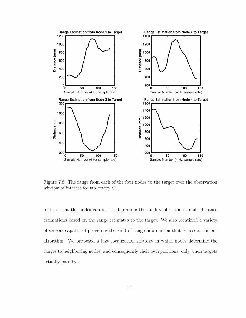
0 50 100 1500

200

400

600

800

1000

1200Range Estimation from Node 1 to Target

Sample Number (4 Hz sample rate)

Dis

tanc

e (m

m)

0 50 100 150200

400

600

800

1000

1200

1400Range Estimation from Node 2 to Target

Sample Number (4 Hz sample rate)

Dis

tanc

e (m

m)

0 50 100 150200

400

600

800

1000

1200Range Estimation from Node 3 to Target

Sample Number (4 Hz sample rate)

Dis

tanc

e (m

m)

0 50 100 150200

400

600

800

1000

1200

1400

1600Range Estimation from Node 4 to Target

Sample Number (4 Hz sample rate)

Dis

tanc

e (m

m)

Figure 7.8: The range from each of the four nodes to the target over the observationwindow of interest for trajectory C.

metrics that the nodes can use to determine the quality of the inter-node distance

estimations based on the range estimates to the target. We also identified a variety

of sensors capable of providing the kind of range information that is needed for our

algorithm. We proposed a lazy localization strategy in which nodes determine the

ranges to neighboring nodes, and consequently their own positions, only when targets

actually pass by.

151

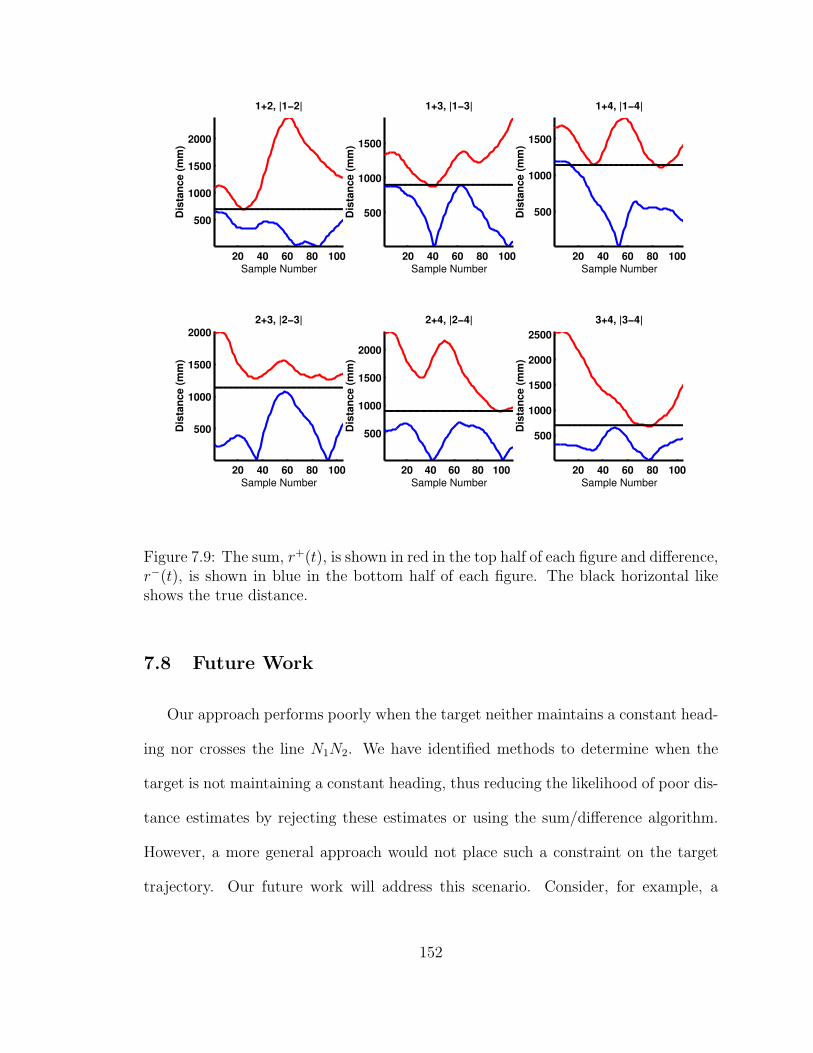
20 40 60 80 100

500

1000

1500

2000

1+2, |1−2|

Sample Number

Dis

tanc

e (m

m)

20 40 60 80 100

500

1000

1500

1+3, |1−3|

Sample Number

Dis

tanc

e (m

m)

20 40 60 80 100

500

1000

1500

1+4, |1−4|

Sample Number

Dis

tanc

e (m

m)

20 40 60 80 100

500

1000

1500

20002+3, |2−3|

Sample Number

Dis

tanc

e (m

m)

20 40 60 80 100

500

1000

1500

2000

2+4, |2−4|

Sample Number

Dis

tanc

e (m

m)

20 40 60 80 100

500

1000

1500

2000

25003+4, |3−4|

Sample Number

Dis

tanc

e (m

m)

Figure 7.9: The sum, r+(t), is shown in red in the top half of each figure and difference,r−(t), is shown in blue in the bottom half of each figure. The black horizontal likeshows the true distance.

7.8 Future Work

Our approach performs poorly when the target neither maintains a constant head-

ing nor crosses the line N1N2. We have identified methods to determine when the

target is not maintaining a constant heading, thus reducing the likelihood of poor dis-

tance estimates by rejecting these estimates or using the sum/difference algorithm.

However, a more general approach would not place such a constraint on the target

trajectory. Our future work will address this scenario. Consider, for example, a

152

Run 1 Run 2 Run 3 Run 4

CPA Error 7cm 11cm 11cm 6cmSum Error 9cm 16cm 4cm 7cmDifference Error 34cm 31cm 20cm 14cm

Table 7.1: A comparison of the cumulative range errors of the CPA, sum, and differ-ence algorithms as function of the number of passing targets.

configuration that allows three independent sensor nodes to range the same target

simultaneously at three distinct points in time, as shown in Figure 7.10.

r 1,3

r 2,3

r 3,3

r 1,1 r 2,1

r 3,1

r 1,2

r 3,2

r 2,2

N 1

N 2 N 3

t 1

t 2

t 3

Trajectory of mobile object

Figure 7.10: The trajectory of a target (yellow dot) and its distance rn,t from threesensor nodes at three points in time, where n is one of N1, N2, and N3, and t is oneof t1, t2, and t3.

The positions of the three nodes N1, N2, and N3 are unknown and we refer to these

nodes as the unknown nodes. Each of these unknown nodes is able to determine the

153

distance to the target at three distinct times t1, t2, and t3. Let us define the range

graph as the planar geometric structure whose six vertices are defined by the location

of three unknown nodes N1, N2, and N3, and of a target at three times t1, t2, and t3,

and whose edges are the nine ranges ri,j. We have proven that the range graph is both

rigid and unique if neither the three nodes nor the three points of the trajectory are

collinear. Solving the resulting quadratically constrained optimization problem will

yield the positions of the three nodes and position of the target at the three times.

154

CHAPTER 8

CONCLUSIONS

This thesis reports on our experiences in performing event detection with wireless

sensor networks. We first presented the key differences between data collection and

event detection, noting, for example their very different energy usage profiles. Our

key observation was that the detection of random events is a fundamentally different

problem from the periodic collection of data and that these differences give rise to

a rich space of tradeoffs and a multitude of opportunities for energy savings. For

example, data collection may allow sensor nodes to sleep most of the time but event

detection requires that sensors be actively or passively vigilant most of the time. On

the other hand, data collection may require frequent messaging to report measure-

ments but event detection may only require reporting when an event actually occurs.

In the case of sensing, data collection is more miserly with energy but in the case of

messaging, event detection may be more miserly with energy. Based on these obser-

vations, we proposed an extreme architecture for random event detection – one that

advocates an entirely event-driven approach.

Using energy as the critical metric, we then presented the design of the eXtreme

Scale Mote (XSM), a novel sensor network platform that includes capabilities for pas-

sive vigilance (low-power wakeup sensing) and recoverability (grenade timer). This

155

new platform extends the event-driven model into sensing by adding an interrupt in-

terface to sensors. We then demonstrated the essential elements of detection and clas-

sification, common to many intrusion detections systems, for ferromagnetic targets.

We noted the challenges of using high-power, low-latency sensors in conjunction with

low-power, high-latency analog signal conditioning circuits and presented the design

of a multi-phase clocked sample-and-hold control circuit for addressing this problem

in the general case. Our design makes it possible to use such sensors for low-power

passive vigilance purposes when, normally, they could not be used in such a manner.

As a counterpoint, we presented the platform design and signal processing algorithms

for an ultrawideband radar sensor. We demonstrated low-complexity algorithms for

signal detection and pattern classification but we did not find the radar sensors well

suited for low-power wakeup purposes due to their high-latency startup calibration

process.

We then extended the event-driven model into the middleware, advocating reac-

tive or post facto protocols for time synchronization, localization, and routing. The

observation that led us in this direction was that when the frequency of random events

is much lower than the peer-to-peer middleware messaging rate, stale state, particu-

larly for protocols like time synchronization and routing, is maintained unnecessarily.

By updating state reactively or post facto, significant energy can be saved and in-

stead used to extend system lifetime. We presented the design of an event-driven

time synchronization algorithm and the both the design and implementation of a re-

active localization algorithm. We admit that our ideas may be difficult to implement

broadly without realizing some technical advances in low-power wakeup sensors and

wakeup radios.

156

We also learned a number of key lessons during the development of the systems

presented in this thesis, as outlined below.

System-building: We took the view that ultimately diverse sensors, algorithms,

platforms, radios, batteries, and other components must be assembled into cohesive

integrated systems to provide value, and that the process of actually building these

systems would teach us a great deal. System-building does come at a very high

cost – both in time and money. For example, the specification, design, prototyping,

evaluation, redesign, and reevaluation of the XSM has already taken more than nine

months and is still continuing. The design effort primarily involved two different in-

stitutions and the evaluation effort involved another half-dozen. Navigating through

the complexities of such distributed teams is especially challenging. And still fur-

ther compounding our difficulties is the special nature of the electronic components

marketplace – allocations, lead times, second sources, and so on. Bringing up a new

platform is expensive and we advocate avoiding this process unless a quantum leap

in features or performance is both needed and unavailable through other avenues.

Noise: Noise is typically modeled as a normally distributed random variable

and samples of this variable are assumed independent and identically distributed

(uncorrelated). Our experience demonstrates that this model frequently fails to holds

in the harsh realities of the great outdoors. We find that noise tends to be wider-

tailed and more correlated than Gaussian and that clutter caused by real objects not

of interest to us is quite prevalent. Correlated noise and clutter can result in false

alarm rates. For example, air thermals can cause false alarms on our passive infrared

sensors, requiring us to extract additional features for distinguish signals from noise.

Since the root cause of the non-Gaussian nature of the noise is unknown, we are forced

157

to deal with the problem in signal processing, where signals are routinely clipped and

filtered to eliminate spikes and lower the false alarm rate. However, we still find

it difficult to differentiate between signals and clutter noise. In such scenarios, a

distributed algorithm is useful since even though the noise is correlated in time at a

point in space, it is unlikely correlated in space at a point in time. By averaging across

space-time, we are able reduce the probability of false alarm. For even greater noise

rejection, we could introduce additional orthogonal sensing modes allowing diversity

in space, time, and signal.

Signal Processing: As a direct consequence of the harshness of the real-world

noise model and the impossibility of attending to individual sensors at scales ap-

proaching 10,000 nodes, the signal processing algorithms must be robust and adaptive.

At the same times, the algorithms are constrained by limited memory, computational

resources, and communications bandwidth. Achieving the desired receiver operating

characteristic (ROC) curve in the face of such system-wide constraints is difficult

and time-consuming. Consequently, we warn future systems designers to be wary

of approaches that trivialize the sensing and signal processing aspects of these net-

works. An acceptable solution, we find, frequently violates desired modularity and

encapusation properties and suffers from poor reuse properties. We must discover

new methods to improve the design of signal processing algorithms for this class of

devices.

Testbeds: We discovered that the data collection aspects of our research were

both time-consuming and overhead-laden. To clarify what we mean by “time-consuming

and overhead-laden,” consider a typical day of testing for collecting two hours of field

data. First, the test site had to be reserved several days in advance since we our test

158

facility was owned by a third party. The remainder of our effort was concentrated on

the actual day of testing, as shown in Figure 8.1.

Figure 8.1: Typical schedule spanning from 9:00 A.M. to 11:30 P.M. for collecting anhour or two of sensor data.

A review of the test day schedule reveals a ten hour overhead for a medium

scale experiment. As a result, we did not test our applications in the field frequently.

159

Instead, we would schedule multi-hour tests followed by multiple days of programming

in the lab to correct errors. There were times during which we made adjustments

to our programs in-the-field because of silly programming mistakes. Other problems

were more difficult to diagnose. For example, we frequently discovered that things

did not work in the field at medium scale even though they did work it the lab at a

smaller scale. In such cases, we had to return to the lab with only the data logs we

had captured but without an efficient mechanism to verify that any particular change

would correct the problem. Consequently, we found the overhead of testing to be far

greater than a few hours – in some cases we spent entire days with no results.

We identified many problems with our testing strategy. The overhead involved in

setting up and tearing down tests was simply too great for us to do testing regularly

and we did not have sufficient visibility into the overall state of the system to analyze

and understand, in a fine-grained manner, what each element of the system was doing

at any given moment. Our tests were not meaningfully repeateable since temperature,

humidity, sunlight, rain, and other factors varied from day to day. The scalability

of our tests were limited by the overhead involved in programming nodes, deploying

and retrieving sensors, and downloading data.

To address these drawbacks to our testing strategy, we have begun construction

of a state-of-the-art automated sensor network testbed. We envision a testbed that

takes as input the program(s) to be tested, the network topology to be used, the

environmental conditions to be simulated, and the behaviors of evader and pursuer

robotic agents. The testbed would provide as output, via an out-of-band communi-

cations channel, a time-stamped history of sent and received messages, all important

state changes in every sensor node, the actual network topology that was used, the

160

timing and sequence of environmental factors, the actual trajectories and actions of

the robotic agents, and an overhead video of the entire testing session. The guiding

principle of our vision is to automate every aspect of the testbed so that experiments

are fast, informative, and repeatable. In a slight variation on this theme, we also

envision supporting Internet-based ad hoc interactive control of both the pursuer and

evader robots while the testbed collects detailed trajectory information about both.

161

CHAPTER 9

FUTURE WORK

9.1 Sensor and Platforms

A number of potential future research directions emerged during the course of

this work. We believe wakeup sensors will become standard on future sensor network

platforms because they extend the inherently more energy-efficient event-driven model

into hardware. In support of such wakeup sensors, we expect future platforms to

integrate increasingly lower-power and more programmable analog signal processing

electronics. For example, programmable differentiators, integrators, detectors, and

automatic gain control circuits may enable passive vigilance with lower false alarm

and power consumption rates than possible today. This trend may lead to dedicated

VLSI signal processors with both analog and digital interfaces. Specialized mixed-

signal circuits may provide extremely fine-grained and synchronized power control,

sampling, filtering, and triggering, all in hardware. Advances in MEMS may enable

zero-power wakeup by directly coupling mechanical energy at the resonant frequencies

of the sensors. Low-power wakeup radios will allow neighboring sensor nodes to

initiate communications even when the processor and main radio is turned off.

162

Once sensor network platforms begin supporting wakeup sensors and radios with

event-driven interfaces, entirely event-driven application approaches will emerge due

to the desire for longer system lifetimes. Communications will become predominantly

reactive rather than proactive. Time synchronization, localization, and link estima-

tion will occur ex post facto. The latency-lifetime tradeoff will incorporate hysteresis:

if there is no event activity for a prolonged period time, then the network will exhibit

a higher latency when reporting the very first event after the period of no activity.

Thereafter, the latency may be positively correlated with the amount of time that

passes before the next event arrives (i.e. latency increases if there is no activity, per-

haps with some important thresholds or in a quantized manner). However, if there is

a constant flurry of event activity, then the network maintains a constant high level

of vigilance and low latency. Dynamically varying latency in this manner supports

power management and is similar to the way adaptive biological systems work.

Future platforms will integrate energy-harvesting subsystems like solar cells. Such

capabilities will allow a sensor node to dynamically govern its own behavior based on

its assigned tasks, energy reserves, and probable future power availability. To this list,

certainly we could add neighbors’ energy reserves as well. The static inputs to such a

“power management” scheme might be the user’s desired level of system performance,

false alarm rate, latency, active vs passive vigilance (or something in between – do the

“best” given the available power reserves or expected future power availability). In

addition, the user might suggest multiple thresholds or ranges of system performance:

ideal, acceptable, minimum. If the node’s performance drops below minimum it

should just go to sleep or increase its vigilance to achieve this level of performance even

163

if it means a premature death. Such a dynamic approach will enable sensor networks

to provide continuous best efforts performance and significantly longer lifetimes.

9.2 Ultrawideband Technologies

Ultrawideband (UWB) technologies will become inexpensive and broadly available

as these technologies become integrated into mainstream applications like wireless net-

working and vehicle collision avoidance. Such applications will drive this technology

toward low-power chip-scale solutions. Researchers, concurrently, will demonstrate

experimental radar-enabled sensor networks with the potential to address key sens-

ing, classification, tracking, time synchronization, localization, and communications

challenges for a variety of security applications including detection, classification, and

tracking. In the future, UWB-enabled sensor networks will determine the range, ve-

locity, tomographic features, and cross-sectional areas of targets from 50m away, syn-

chronize network time on pico-second scales, estimate ranges to neighboring nodes at

sub-centimeter accuracies, and communicate at megabit-rates. UWB radar-enabled

sensor networks will provide this new level of functionality and performance at mil-

liwatt power levels, with low probability of detect or intercept, and with modest

algorithmic space, time, and message complexity.

9.3 Tool Support for Signal Processing

Designing appropriate signal processing algorithms consumed a significant amount

of our time. There are four factors which contributed to making this task so diffi-

cult. First, data collection is itself quite time-consuming. Second, the physical world

164

exhibits great variability which causes noise and clutter that is difficult to discrimi-

nate from signals of interest. The decision boundary is particularly difficult when the

probabilities of detection and false alarm are constrained. Third, the limited energy

reserves of many sensor network nodes preclude classical signal processing algorithms

which have high space, time, or message cost. Fourth, signal processing is itself a com-

plex topic which is made even more difficult when saddled with the highly-coupled

system-wide constraints encountered in sensor networks.

Novel signal processing algorithm and tools will be developed as sensor networks

are increasingly used to monitor random phenomena. Future research might focus

on automating the analysis, system identification, and automated code generation of

signal processing chains. Users would upload long time series of data into these tools

and would specify available power budget and the energy cost of various operations.

The tools would then, perhaps using some user supplied hints, automatically cluster

the data based a set of statistics. Relevant clusters of the data would be labeled

appropriately by the user and the tool would automatically generate software algo-

rithms to identify the presence of this data. The algorithms would be constrained

by the available memory, processing power, and communications ability of the sensor

nodes.

9.4 Applications

Many non-military event detection applications will emerge in the future. Re-

searchers are investigating applications of wireless sensor networks for traffic surveil-

lance, structural health monitoring, and distributed earthquake monitoring. Traffic

surveillance, in particular, represents a rich class of sensor network applications with

165

enormous potential benefits for society. Novel approaches based on a distributed

computing model that performs in situ information processing, aggregation, and ex-

filtration is promising. A distributed approach to traffic surveillance could improve

travel time estimation, allow rapid incident detection, and provide typical traffic pa-

rameters including flow, speed, and density.

The instrumentation of the traffic facility with a network of sensors is not a new

concept. Most metropolitan areas have sophisticated traffic management systems for

monitoring the roadways. However, today’s systems distribute the data collection

function throughout the facility, but perform highly centralized data processing. As

a result, these systems produce and transmit enormous volumes of data, frequently

over expensive communication channels. Much of the data that are transmitted are

used to perform near-real-time computations to obtain salient and actionable traffic

management data, but the data are then discarded. Sensor networks will allow this

processing to take place within the network, and only interesting event data will be

forwarded to the traffic management center.

Reliably determining whether the traffic state is free flowing or congested is consid-

ered the most important function of a traffic surveillance system but this requirement

is difficult to implement with today’s prevailing detector technologies that only mon-

itor the traffic state at sparse points along the roadway. Since traffic incidents can

occur at any point on the roadway, but can only be detected with today’s sparsely

distributed sensors, incidents may go unnoticed for long periods of time. Incident de-

tection is also possible by monitoring backward- and forward-moving “shockwaves”

that radiate from congested regions but the backward-moving shockwaves generated

by a queue move at a fraction of the free flow speed possibly causing critical minutes

166

to elapse between the time that an incident occurs and when it is detected. Down-

stream or forward-moving shockwaves travel more quickly but they are less reliable

than upstream shockwaves as indicators of congestion.

Wireless sensor networks can be applied to the problem of determining whether

the traffic facility is free flowing or congested. By aggregating traffic flow in a fine-

grained and highly-distributed manner across all lanes, including any egress or ingress

lanes, we may be able to accurately identify traffic state changes in near real-time. A

densely distributed sensor network can determine the traffic state and detect traffic

incidents faster than today’s approaches due to the finer granularity with which sensor

networks can monitor the traffic facility.

We envision a traffic surveillance model in which vehicle trajectory data are pro-

cessed locally in a dense network of sensors and shared with neighboring sensors

that are upstream, downstream, and in adjacent lanes. Our motivation comes from

the apparent spatial- and temporal-locality of traffic state perturbations, suggesting

a distributed approach that allows individual sensor nodes, or clusters of nodes, to

perform localized processing, filtering, and triggering functions. Collaborative signal

processing may enable more complex data sampling, aggregation, and compression

than is possible with an individual node.

A distributed traffic surveillance system could provide significant benefits over ex-

isting systems. By distributing the computing throughout the traffic facility, we can

increase local processing and aggregation while simultaneously reducing the need the

to transmit enormous volumes of information that quickly are discarded. A densely

distributed network of sensors also enables much faster, and more local, congestion

detection than is possible today enabling us to improve travel time estimation, allow

167

rapid incident detection, and provide typical traffic parameters including flow, speed,

and density. Ultimately, by instrumenting the traffic facility and dynamically rerout-

ing traffic, we may be able to significantly reduce travel delay and lower the cost of

traffic congestion which resulted in a $67 billion burden on the U.S. economy in 2000

[65].

The high capital and operating expenses associated with current traffic surveil-

lance technologies, especially when compared to the limited value they provide, gives

us an economic incentive to develop sensor networks for traffic surveillance.

168

APPENDIX A

ELECTRICAL SCHEMATICS

169

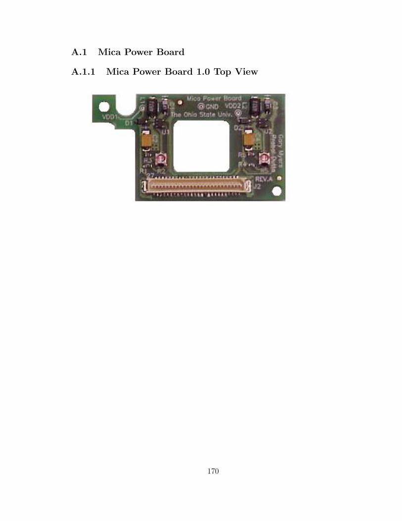
A.1 Mica Power Board

A.1.1 Mica Power Board 1.0 Top View

170

A.1.2 Mica Power Board 1.0 Schematic

5 5

4 4

3 3

2 2

1 1

DD

CC

BB

AA

AD

C7

VD

D2

PW

M1B

AD

C5

FLA

SH

_CLK

Littl

e_G

uy_S

PI_

Clo

ck

PW

2

AD

C2

INT0

INT1

AC

-

INT2

Littl

e_G

uy_R

eset

FLA

SH

SO

LED

2

INT3

VD

D1

RES

ET

PW

3

FLA

SH

SI

PW

7

gnd_

anal

og

PW

4

Littl

e_G

uy_M

ISO

DC

_BO

OS

T_S

HU

TDO

WN

PW

5

AD

C3

AD

C4

PW

0

I2C

_BU

S_1

_CLK

ALERD

PW

1

LED

1

PW

M0

PR

OG

_MO

SI_

SPI

PW

6LE

D3

Littl

e_G

uy_M

OS

I

AC

+

I2C

_BU

S_1

_DAT

A

WR

AD

C6

AD

C1

AD

C0_

BB

Out

Vcc

PW

0

VD

D1

VD

D2

Vcc

PW

1

PW

4P

W5

PW

0

Littl

e_G

uy_M

ISO

PW

2P

W1

Littl

e_G

uy_M

OS

I

UAR

T_TX

D0

Littl

e_G

uy_R

eset

UA

RT_

RXD

0

PW

6

Littl

e_G

uy_S

PI_

Clo

ck

PW

3

RES

ET

Vcc

PW

M1B

AD

C6

AD

C2

AD

C4

AD

C5

AD

C3

AD

C0_

BB

Out

AD

C7

AD

C1

PW

M1A

PR

OG

_MIS

O_S

PIS

CK

_SP

I

AC

+P

WM

1A

gnd_

anal

og

LED

3

FLA

SH

_CLK

FLA

SH

SO

DC

_BO

OS

T_S

HU

TDO

WN

LED

1R

D

I2C

_BU

S_1

_CLK

INT0

PW

7

WR

AC

-

PW

M0

I2C

_BU

S_1

_DAT

A

PR

OG

_MIS

O_S

PI

INT1

INT2

ALE

PR

OG

_MO

SI_

SPI

SC

K_S

PI

VD

D_A

NA

LOG

FLA

SH

SI

LED

2

INT3

UA

RT_

RXD

0U

ART_

TXD

0

Title

Size

Doc

umen

t Num

ber

Rev

Dat

e:S

heet

of

Prab

al D

utta

, The

Ohi

o St

ate

Uni

vers

ity1

Mic

a Po

wer

Boa

rdC

11

Sat

urda

y, M

ay 0

3, 2

003

Connector(Bottom)

Connector(Top)

NOTE:TheMicaPowerBoard("MICAPB")isdesignedto

interfacewiththeMICA,MICA2,andMICASBontheBOTTOM

connector.TheVDD_ANALOGandVccareNOTconnected

straightthroughlikeinmostMICAdaughterboards.

Instead,thesesignalsarereplacedwiththeoutputsoftwo

adjustableDC-DCconverterslabeledVDD1andVDD2.

RecommendedParts:

L1,L2:MurataLQH3C4R7M24orSumidaCD43-4R7

C1,C3:AVXTAJA156M010(CASEA)

C2,C4:AVXTAJB226M006(CASEB)

D1,D2:MBR0520(SOD123)

VDD1=1.23(1+R1a/R1);

R1aistophalfofR1

VDD2=1.23(1+R2a/R2);

R2aistophalfofR2

R2,R5:PANASONICEVM-7JSX30BQ4

R3

TBD

R5

47K

D1

C3

15uF

U1

LT16

13

SW1

GND 2

SHD

N4

FB3

VIN

5

R4

TBD

HIROSESOCKET

J1 1 2 3 4 5 6 7 8 9 10 11 12 13 14 15 16 17 18 19 20 21 22 23 24 25

5253

26

27 28 29 30 31 32 33 34 35 36 37 38 39 40 41 42 43 44 45 46 47 48 49 50 51

U2

LT16

13

SW1

GND 2

SHD

N4

FB3

VIN

5

R2

47K

HIROSEPLUG

J2 1 2 3 4 5 6 7 8 9 10 11 12 13 14 15 16 17 18 19 20 21 22 23 24 25

52

53

26

27 28 29 30 31 32 33 34 35 36 37 38 39 40 41 42 43 44 45 46 47 48 49 50 51

C1

15uF

D2

C2

22uF

R6

TBD

R1

TBD

L1 4.7u

H

L2 4.7u

H

C4

22uF

171

A.2 XSM 1.0

172

A.2.1 XSM 1.0 Top View

173

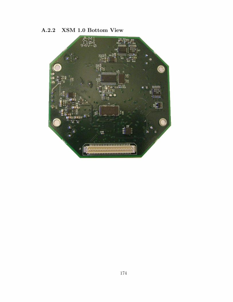
A.2.2 XSM 1.0 Bottom View

174

A.2.3 Acoustic Subsystem

5 5

4 4

3 3

2 2

1 1

DD

CC

BB

AA

MICR

OPHO

NE/S

OUNDER

6310

-033

6-01

A

XS

M10

0CA

XT

RE

ME

SC

ALE

MO

TE

Cro

ssbo

w T

echn

olog

y41

Dag

gett

Driv

eS

an J

ose,

CA

. 951

34

B1

7T

uesd

ay, F

ebru

ary

24, 2

004

X

XX/X

X/XX

2-3-

03

XX/X

X/XX

M. G

RIM

ME

R

X

M. G

RIM

ME

R2-

3-03

Titl

e

Siz

eD

ocum

ent N

umbe

rR

ev

Dat

e:S

heet

of

EX

CE

PT

AS

MA

Y B

E O

TH

ER

WIS

E P

RO

VID

ED

BY

CO

NT

RA

CT,

TH

ISD

RA

WIN

G O

R S

PE

CIF

ICA

TIO

N IS

TH

E P

RO

PR

IETA

RY

PR

OP

ER

TY O

FC

RO

SS

BO

W T

EC

HN

OLO

GY

INC

. IT

IS IS

SU

ED

IN S

TRIC

T C

ON

FID

EN

CE

AN

D S

HA

LL N

OT

BE

RE

PR

OD

UC

ED

OR

CO

PIE

D O

R U

SE

D (P

AR

TIA

LLY

OR

WH

OLL

Y)

IN A

NY

MA

NN

ER

WIT

HO

UT

PR

IOR

EX

PR

ES

S W

RIT

TEN

AU

THO

RIZ

ATI

ON

OF

CR

OS

SB

OW

TE

CH

NO

LOG

Y IN

C.

DA

TE

DW

N

CH

K

AP

RV

D

AP

RV

D

VR

EF

VR

EF

VR

EF

VS

W-

VS

W+

PW

3

PW

2

AD

C2

AU

DIO

_RX

_PW

R

AU

DIO

_RX

_PW

RA

UD

IO_R

X_P

WR

AU

DIO

_RX

_PW

RA

UD

IO_R

X_P

WR

PW

7

PW

M1B

PW

[0..7

]

PW

[0..7

]

PW

M1A

I2C

_CLK

I2C

_DA

TA

PW

[0..7

]

AC

-AD

C[0

..7]

VC

C

VC

C

VC

C

C71

0.1u

F

Q1 ZX

M61

P03

F

1

32

C9

2.2U

F

C13

2.2U

F

C2 1u

F

R5

1.10

K

Q2 ZX

M61

P03

F

1

32

R10

100K

U21

A

AD

5242

2 3 4

6789 10

1

A1

W1

B1

SD

SC

LS

DA

AD

0A

D1

O1

V+ V-

+ -

U5

LM82

612

31

5

4

+ -

V+ V-

U2

MA

X44

66

1 34

5 2

R68

100K

C10

.1uF

R11

56.0

K

C1

10uF

C6

10uF

C11

.1uF

R13

2.21

K

C8

.033

uF

R6

1.10

K

C12

2.2U

F

PZ

1 BU

ZZ

ER

1 2

U22

MA

X74

13E

UA

67

548

132

OS

SH

DN

OU

TV

+C

LK

CO

MG

ND

IN

C3

1uF

C7

0.22

uF

R2

1.10

K

C4

1uF

+ -

V+ V-

U1

MA

X44

66

1 34

5 2

Q5 ZX

M61

P03

F

1

32

U6 M

AX

864

2 4

108 91

15

16

5

12

1413

67

C2+ C2-

NC

FC

0

NC

C1-

V+

C1+

V-

IN

NC

NC

SH

DN

FC

1

R1

100K

U21

B

AD

5242

16 15 14 13125 11

A2

W2

B2

O2

VS

S

VC

C

GN

D

R3

1.10

K

C14

2.2U

F

C5

1uF

R8

5.1K

D1

SD

M10

K45

MM

1

MIC

1 2

R12

100K

R4

100K

R7

1.10

K

V+ V-

+ -

U3

LMC

7215

5

31

2

4R

910

0K

175

A.2.4 XSM 1.0 Power, Accelerometer, and LEDs

5 5

4 4

3 3

2 2

1 1

DD

CC

BB

AA

POWE

R/AC

CEL/

LEDS

6310

-033

6-01

A

XS

M10

0CA

XT

RE

ME

SC

ALE

MO

TE

Cro

ssbo

w T

echn

olog

y41

Dag

gett

Driv

eS

an J

ose,

CA

. 951

34

B2

7T

uesd

ay, F

ebru

ary

24, 2

004

X

XX/X

X/XX

2-3-

03

XX/X

X/XX

M. G

RIM

ME

R

X

M. G

RIM

ME

R2-

3-03

Titl

e

Siz

eD

ocum

ent N

umbe

rR

ev

Dat

e:S

heet

of

EX

CE

PT

AS

MA

Y B

E O

TH

ER

WIS

E P

RO

VID

ED

BY

CO

NT

RA

CT,

TH

ISD

RA

WIN

G O

R S

PE

CIF

ICA

TIO

N IS

TH

E P

RO

PR

IETA

RY

PR

OP

ER

TY O

FC

RO

SS

BO

W T

EC

HN

OLO

GY

INC

. IT

IS IS

SU

ED

IN S

TRIC

T C

ON

FID

EN

CE

AN

D S

HA

LL N

OT

BE

RE

PR

OD

UC

ED

OR

CO

PIE

D O

R U

SE

D (P

AR

TIA

LLY

OR

WH

OLL

Y)

IN A

NY

MA

NN

ER

WIT

HO

UT

PR

IOR

EX

PR

ES

S W

RIT

TEN

AU

THO

RIZ

ATI

ON

OF

CR

OS

SB

OW

TE

CH

NO

LOG

Y IN

C.

DA

TE

DW

N

CH

K

AP

RV

D

AP

RV

D

AD

C4

AD

C3

PW

4

PW

0

PW

1

INT

2

INT

3

PW

[0..7

]

AD

C[0

..7]

PW

M0

PW

M1C

PW

[0..7

]

INT

[0..3

]

VC

C

VC

C

R23

330K

C17

.1uF

R16 0

OH

M

D10

RE

D

SW

1

SP

DT

12

3

U8

AD

XL2

02A

E

1 2 3

45 67

8

ST

T2

GN

D

YO

UT

XO

UT

YF

ILT

XF

ILT

VC

C

R70

470

D6

RE

D

D11

RE

D

R22

100

R74

470

C16

.1uF

R69

470

C18

.1uF

D7

RE

D

R21

1K

R20 0

OH

M

D2 BA

T54

C

R72

470

BT1

BA

TT

ER

Y_2

AA

1

2

V-

V+

D8

RE

D

J6 HD

R 2

X 1

X .1

1 21 2

C19

.1uF

R71

470

C15

.1uF

R73

470

D9

RE

D

176

A.2.5 XSM 1.0 Radio Subsystem

5 5

4 4

3 3

2 2

1 1

DD

CC

BB

AA

50 OHM LINES

50 OHM LINES

50 OHM LIN

ES

L5 L2 L3 L4 C12

C13

C15

C17

REFDES

900 MHZ

433 MHZ

4.7NH

120NH

2.7NH

4.7NH

10PF

-- 10PF

10PF

12NH

68NH

6NH

33NH

15PF

8PF

20PF

20PF

315 MHZ

15NH

39NH

20NH

56NH

8PF

2.2PF

30PF

30PF

RADI

O

6310

-033

6-01

A

XS

M10

0CA

XT

RE

ME

SC

ALE

MO

TE

Cro

ssbo

w T

echn

olog

y41

Dag

gett

Driv

eS

an J

ose,

CA

. 951

34

B3

7T

uesd

ay, F

ebru

ary

24, 2

004

X

XX/X

X/XX

2-3-

03

XX/X

X/XX

M. G

RIM

ME

R

X

M. G

RIM

ME

R2-

3-03

Titl

e

Siz

eD

ocum

ent N

umbe

rR

ev

Dat

e:S

heet

of

EX

CE

PT

AS

MA

Y B

E O

TH

ER

WIS

E P

RO

VID

ED

BY

CO

NT

RA

CT,

TH

ISD

RA

WIN

G O

R S

PE

CIF

ICA

TIO

N IS

TH

E P

RO

PR

IETA

RY

PR

OP

ER

TY O

FC

RO

SS

BO

W T

EC

HN

OLO

GY

INC

. IT

IS IS

SU

ED

IN S

TRIC

T C

ON

FID

EN

CE

AN

D S

HA

LL N

OT

BE

RE

PR

OD

UC

ED

OR

CO

PIE

D O

R U

SE

D (P

AR

TIA

LLY

OR

WH

OLL

Y)

IN A

NY

MA

NN

ER

WIT

HO

UT

PR

IOR

EX

PR

ES

S W

RIT

TEN

AU

THO

RIZ

ATI

ON

OF

CR

OS

SB

OW

TE

CH

NO

LOG

Y IN

C.

DA

TE

DW

N

CH

K

AP

RV

D

AP

RV

D

PA

LE

PD

AT

A

DC

LK

DC

LK

SP

I_S

CK

PC

LKP

DA

TA

PA

LE

AD

C0

SP

I_M

ISO

CH

P_O

UT

AV

CC

AV

CC

VC

C

VC

C

AV

CC

VC

C

AV

CC

VC

C

L4 33nH

C31

1000

pF

C27

15pF

J3

HD

R 2

X 1

X .1

1 21 2

C32

22pF

U9

CC

1000

21

15915

3 4

10 11

12

1318 17

23 24 25 26 2728

VCC

AVCCAVCCAVCCAVCC

RF_

IN

RF

_OU

T

L1 L2

CH

P_O

UT

R_B

IAS

XO

SC

1X

OS

C2

DIO

DC

LKP

CLK

PD

AT

AP

ALE

RS

SI

C20

.033

uFC

2110

00pF

L5 10nH

R29

82.5

K

C24

220p

F

C33

4.7p

F

R25

1M

C30

22pF

C22

1000

pF

C34

13pF

Y1

14.7

456M

HZ

21

21

R26

1M

C29

4.7p

F

C25

.033

uF

C35

13pF

C28

8.0p

F

L2 68nH

R24

1M

C26

1000

pF

C23

220p

F

R28

27.4

K

L3 6.8N

H

L1

BE

AD

-080

5

R27

10K

177

A.2.6 XSM 1.0 Expansion Connector

5 5

4 4

3 3

2 2

1 1

DD

CC

BB

AA

PIN

NAME

DESCRIPTIO

N

1 2 3 4 5 6 7 8 9 10 11 12 13 14 15 16 17 18 19 20 21 22 23 24 25 26

GND

VSNSR

INT3

INT2

INT1

INT0

BAT_MON

LED3

LED2

LED1

RD WR ALE

PW7

USART1_CLK

PROG_MOS

IPROG_MIS

OSPI_SCK

USART1_RXD

USART1_TXD

I2C_CLK

I2C_DATA

PWM0

PWM1A

AC+

AC-

GROUND

SENSOR SUPPLY

GPIO

GPIO

GPIO

GPIO

BATTERY VOLTAGE MONITOR ENABLE

LED3

LED2

LED1

GPIO

GPIO

GPIO

POWER CONTROL 7

USART1 CLOCK

SERIAL PROGRAM M

OSI

SERIAL PROGRAM M

ISO

SPI SERIAL CLO

CKUSART1 RX DA

TAUSART1 TX DA

TAI2C BUS CLOCK

I2C BUS DATA

GPIO/PWM

0GPIO/PWM1A

GPIO/AC+

GPIO/AC-

UART_RXD0

UART_TXD0

PW0

PW1

PW2

PW3

PW4

PW5

PW6

ADC7

ADC6

ADC5

ADC4

ADC3

ADC2

ADC1

ADC0

THERM_PWR

THRU1

THRU2

THRU3

RSTN

PWM1B

VCC

GND

NAME

27 28 29 30 31 32 33 34 35 36 37 38 39 40 41 42 43 44 45 46 47 48 49 50 51PIN

DESCRIPTIO

N

UART_0 RECEI

VEUART_0 TRANSMIT

POWER CONTROL 0

POWER CONTROL 1

POWER CONTROL 2

POWER CONTROL 3

POWER CONTROL 4

POWER CONTROL 5

POWER CONTROL 6

ADC INPUT 7 - BATTERY MONITOR/JTAG TDI

ADC INPUT 6 / JTAG

TDO

ADC INPUT 5 / JTAG

TMS

ADC INPUT 4 / JTAG

TCK

ADC INPUT

3ADC INPUT

2ADC INPUT

1ADC INPUT 0 / RSSI MON

ITOR

TEMP SENSOR ENABLE

THRU CONNECT

1THRU CONNECT

2THRU CONNECT3

RESET (NEG

)GPIO/PWM1B

DIGITAL SUPP

LYGROUND

PROG_MOS

IPROG_MISO

MOTE

CON

NECTOR

6310

-033

6-01

A

XS

M10

0CA

XT

RE

ME

SC

ALE

MO

TE

Cro

ssbo

w T

echn

olog

y41

Dag

gett

Driv

eS

an J

ose,

CA

. 951

34

B4

7T

uesd

ay, F

ebru

ary

24, 2

004

X

XX/X

X/XX

2-3-

03

XX/X

X/XX

M. G

RIM

ME

R

X

M. G

RIM

ME

R2-

3-03

Titl

e

Siz

eD

ocum

ent N

umbe

rR

ev

Dat

e:S

heet

of

EX

CE

PT

AS

MA

Y B

E O

TH

ER

WIS

E P

RO

VID

ED

BY

CO

NT

RA

CT,

TH

ISD

RA

WIN

G O

R S

PE

CIF

ICA

TIO

N IS

TH

E P

RO

PR

IETA

RY

PR

OP

ER

TY O

FC

RO

SS

BO

W T

EC

HN

OLO

GY

INC

. IT

IS IS

SU

ED

IN S

TRIC

T C

ON

FID

EN

CE

AN

D S

HA

LL N

OT

BE

RE

PR

OD

UC

ED

OR

CO

PIE

D O

R U

SE

D (P

AR

TIA

LLY

OR

WH

OLL

Y)

IN A

NY

MA

NN

ER

WIT

HO

UT

PR

IOR

EX

PR

ES

S W

RIT

TEN

AU

THO

RIZ

ATI

ON

OF

CR

OS

SB

OW

TE

CH

NO

LOG

Y IN

C.

DA

TE

DW

N

CH

K

AP

RV

D

AP

RV

D

UA

RT

_TX

D0

UA

RT

_RX

D0

SP

I_S

CK

RS

TN

UA

RT

_TX

D0

UA

RT

_RX

D0

VC

C

VC

C

M3

MTG

128

11

HIROSE PLUG

J5

DF

9-51

P-1

V(5

4)

1 2 3 4 5 6 7 8 9 10 11 12 13 14 15 16 17 18 19 20 21 22 23 24 25 26

27 28 29 30 31 32 33 34 35 36 37 38 39 40 41 42 43 44 45 46 47 48 49 50 51

M4

MTG

128

11

M1

MTG

128

11

M2

MTG

128

11

178

A.2.7 XSM 1.0 Microcontroller and Memory Subsystem

5 5

4 4

3 3

2 2

1 1

DD

CC

BB

AA

CPU/

FLAS

H/SE

RIAL ID

6310

-033

6-01

A

XS

M10

0CA

XT

RE

ME

SC

ALE

MO

TE

Cro

ssbo

w T

echn

olog

y41

Dag

gett

Driv

eS

an J

ose,

CA

. 951

34

B5

7T

uesd

ay, F

ebru

ary

24, 2

004

X

XX/X

X/XX

2-3-

03

XX/X

X/XX

M. G

RIM

ME

R

X

M. G

RIM

ME

R2-

3-03

Titl

e

Siz

eD

ocum

ent N

umbe

rR

ev

Dat

e:S

heet

of

EX

CE

PT

AS

MA

Y B

E O

TH

ER

WIS

E P

RO

VID

ED

BY

CO

NT

RA

CT,

TH

ISD

RA

WIN

G O

R S

PE

CIF

ICA

TIO

N IS

TH

E P

RO

PR

IETA

RY

PR

OP

ER

TY O

FC

RO

SS

BO

W T

EC

HN

OLO

GY

INC

. IT

IS IS

SU

ED

IN S

TRIC

T C

ON

FID

EN

CE

AN

D S

HA

LL N

OT

BE

RE

PR

OD

UC

ED

OR

CO

PIE

D O

R U

SE

D (P

AR

TIA

LLY

OR

WH

OLL

Y)

IN A

NY

MA

NN

ER

WIT

HO

UT

PR

IOR

EX

PR

ES

S W

RIT

TEN

AU

THO

RIZ

ATI

ON

OF

CR

OS

SB

OW

TE

CH

NO

LOG

Y IN

C.

DA

TE

DW

N

CH

K

AP

RV

D

AP

RV

D

FLA

SH

_CS

SE

RIA

L_ID

PW

7P

W6

PW

5P

W4

PW

3P

W2

PW

1P

W0

US

AR

T1_

RX

D

SE

RIA

L_ID

US

AR

T1_

CLK

US

AR

T1_

TX

D

UA

RT

_TX

D0

US

AR

T1_

RX

D

LED

3LED

2

LED

1

FLA

SH

_CS

FLA

SH

_CS

SP

I_M

OS

IA

DC

3

AD

C5

AD

C4

AD

C0

AD

C6

AD

C2

AD

C7

AD

C1

INT

1IN

T2

INT

3

INT

0

INT

0IN

T[0

..3]

FLA

SH

_CS

US

AR

T1_

TX

DU

SA

RT

1_C

LKU

SA

RT

1_R

XD

PC

LKP

DA

TA

LED

3LE

D2

LED

1

MA

G_S

RC

HP

_OU

TT

HE

RM

_PW

RP

W[0

..7]

SP

I_S

CK

PW

M0

PW

M1A

PW

M1B

RS

TN

INT

[0..3

]

UA

RT

_RX

D0

UA

RT

_TX

D0

AC

-

AD

C[0

..7]

WR

RD

ALE

SP

I_M

ISO

I2C

_CLK

I2C

_DA

TA

US

AR

T1_

RX

DU

SA

RT

1_T

XD

PA

LEU

SA

RT

1_C

LK

AC

+

PW

M1C

VC

C

VC

C

VC

C

VC

C

VC

C

VC

C

VC

C

VS

NS

R

VC

C

VC

CV

CC

C46

1000

pF

U12 DS

2401

P

2D

Q

R33

0 O

HM

C43

.1uF

C47

1000

pF

C39

.01u

F

C44

.1uF

R36

10K

R34

1M

D4

GR

EE

N

12

R31

10K

C40

.01u

F

C51

13pF

C38

.01u

F

C45

.1uF

C73

0.1u

F

50V

10%

R32

1M

D3

RE

D

12

R38

470

Y2

7.37

28M

HZ

2 341

X2

X2

X1

X1

C36

10uF

6.3V

Y3

32.7

68K

HZ21

34

C48

1000

pF

R40

470

C37

.01u

F

U20

AT

45D

B16

1B

12 3456

7

8 9 10 11 12 13 14 151617181920212223

2425 262728

GN

DN

CN

C

CS

SC

KS

IS

O

NC

NC

NC

NC

NC

NC

NC

NC

NC

NC

NC

NC

NC

NC

NC

RD

YR

ST

WP

NC

NC

VC

C

D5

YE

LLO

W

12

C41

.01u

F

R67

10.0

K

SW

2

PB

SP

ST

12

53 4

R30

470

R37

4.7K

U10

AT

ME

GA

128L

51 50 49 48 47 46 45 44 10 11 12 13 14 15 16 1735 36 37 38 39 40 41 42

25 26 27 28 29 30 31 32 2 3 4 5 6 7 8 9 61 60 59 58 57 56 55 54

6462

1

202423

33 34 43

1819

PA

0/A

D0

PA

1/A

D1

PA

2/A

D2

PA

3/A

D3

PA

4/A

D4

PA

5/A

D5

PA

6/A

D6

PA

7/A

D7

PB

0/S

SP

B1/

SC

KP

B2/

MO

SI

PB

3/M

ISO

PB

4/O

C0

PB

5/O

C1A

PB

6/O

C1B

PB

7/O

C1C

PC

0/A

8P

C1/

A9

PC

2/A

10P

C3/

A11

PC

4/A

12P

C5/

A13

PC

6/A

14P

C7/

A15

PD

0/I2

C_C

LKP

D1/

I2C

_DA

TA

PD

2/R

XD

1P

D3/

TX

D1

PD

4/IC

1P

D5/

XC

K1

PD

6/T

1P

D7/

T2

PE

0/R

XD

0P

E1/

TX

D0

PE

2/X

CK

0P

E3/

OC

3AP

E4/

OC

3BP

E5/

OC

3CP

E6/

T3

PE

7/IC

3

PF

0/A

DC

0P

F1/

AD

C1

PF

2/A

DC

2P

F3/

AD

C3

PF

4/T

CK

PF

5/T

MS

PF

6/T

DO

PF

7/T

DI

AVCCAREF

PE

N

RSTXTAL1XTAL2

PG

0/W

RP

G1/

RD

PG

2/A

LE

PG3/TOSC2PG4/TOSC1

C49

1000

pF

U11

AT

45D

B04

1

1 2 3 458

SI

SC

KR

ST

CS

WP

SO

R35

10K

C50

13pF

C42

.01u

F

R39

470

179

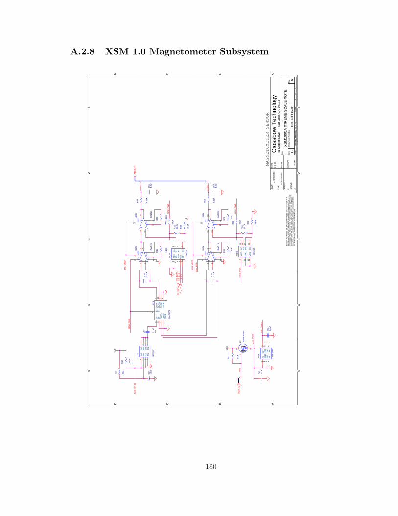
A.2.8 XSM 1.0 Magnetometer Subsystem

5 5

4 4

3 3

2 2

1 1

DD

CC

BB

AA

MAGN

ETOM

ETER

SENSOR

6310

-033

6-01

A

XS

M10

0CA

XT

RE

ME

SC

ALE

MO

TE

Cro

ssbo

w T

echn

olog

y41

Dag

gett

Driv

eS

an J

ose,

CA

. 951

34

B6

7T

uesd

ay, F

ebru

ary

24, 2

004

X

XX/X

X/XX

2-3-

03

XX/X

X/XX

M. G

RIM

ME

R

X

M. G

RIM

ME

R2-

3-03

Titl

e

Siz

eD

ocum

ent N

umbe

rR

ev

Dat

e:S

heet

of

EX

CE

PT

AS

MA

Y B

E O

TH

ER

WIS

E P

RO

VID

ED

BY

CO

NT

RA

CT,

TH

ISD

RA

WIN

G O

R S

PE

CIF

ICA

TIO

N IS

TH

E P

RO

PR

IETA

RY

PR

OP

ER

TY O

FC

RO

SS

BO

W T

EC

HN

OLO

GY

INC

. IT

IS IS

SU

ED

IN S

TRIC

T C

ON

FID

EN

CE

AN

D S

HA

LL N

OT

BE

RE

PR

OD

UC

ED

OR

CO

PIE

D O

R U

SE

D (P

AR

TIA

LLY

OR

WH

OLL

Y)

IN A

NY

MA

NN

ER

WIT

HO

UT

PR

IOR

EX

PR

ES

S W

RIT

TEN

AU

THO

RIZ

ATI

ON

OF

CR

OS

SB

OW

TE

CH

NO

LOG

Y IN

C.

DA

TE

DW

N

CH

K

AP

RV

D

AP

RV

D

MA

G_V

RE

F

MA

G_P

WR

MA

G_V

RE

F

MA

G_P

WR

MA

G_P

WR

AD

C6

AD

C5

MA

G_V

RE

F

MA

G_P

WR

MA

G_P

WR

MA

G_P

WR

PW

5I2

C_C

LKI2

C_D

AT

A

PW

5

MA

G_S

RA

DC

[0..7

]

PW

[0..7

]

I2C

_DA

TA

I2C

_CLK

VC

C VC

C

C58

1.0u

F

U15

HM

C10

52

1234

5

6 78

910

GN

DB

OU

TB

+G

ND

A1

OU

TA

+

VBR

SR

+

OU

TB

-

SR

-

GN

DA

2

OU

TA

-

U17

A

AD

5242

2 3 4

6789 10

1

A1

W1

B1

SD

SC

LS

DA

AD

0A

D1

O1

C56

1.0u

F

C55

1.0u

F

R49

39.2

K R47

39.2

K

R51

1.10

KR

53

39.2

K

C52

1.0u

F

R43

100K

GAINSNS

VREF

U13

B

INA

2126

15 16

13

14

1110

12

U16 TLE

2426

123 4 5

678O

UT

GN

DIN N

CN

CN

CN

CN

R

GAIN

V+ V-

SNS

VREF

U18

A

INA

2126

2 1

4

3

9 8

67

5

R52

1.10

K

U14

IRF

7507

12345 6 7 8

SN

GN

SP

GP

DP

DP

DN

DN

R44

8.25

K

U17

B

AD

5242

16 15 14 13125 11

A2

W2

B2

O2

VS

S

VC

C

GN

D

R41

200

C53

0.1u

F25

V

C57

1.0u

F

R55

39.2

K

C54

1.0u

F

R50

8.25

K

R48 20.0

K

Q3 ZX

M61

P03

F

1

32

R45

1.10

K

GAIN

V+ V-

SNS

VREF

U13

A

INA

2126

2 1

4

3

9 8

67

5C

6510

uF

GAINSNS

VREF

U18

B

INA

2126

15 16

13

14

1110

12

R54 20.0

K

R46

1.10

K

R42

10.0

K

180

A.2.9 XSM 1.0 Passive Infrared Subsystem

5 5

4 4

3 3

2 2

1 1

DD

CC

BB

AA

PIR

SENS

OR

6310

-033

6-01

A

XS

M10

0CA

XT

RE

ME

SC

ALE

MO

TE

Cro

ssbo

w T

echn

olog

y41

Dag

gett

Driv

eS

an J

ose,

CA

. 951

34

B7

7T

uesd

ay, F

ebru

ary

24, 2

004

X

XX/X

X/XX

2-3-

03

XX/X

X/XX

M. G

RIM

ME

R

X

M. G

RIM

ME

R2-

3-03

Titl

e

Siz

eD

ocum

ent N

umbe

rR

ev

Dat

e:S

heet

of

EX

CE

PT

AS

MA

Y B

E O

TH

ER

WIS

E P

RO

VID

ED

BY

CO

NT

RA

CT,

TH

ISD

RA

WIN

G O

R S

PE

CIF

ICA

TIO

N IS

TH

E P

RO

PR

IETA

RY

PR

OP

ER

TY O

FC

RO

SS

BO

W T

EC

HN

OLO

GY

INC

. IT

IS IS

SU

ED

IN S

TRIC

T C

ON

FID

EN

CE

AN

D S

HA

LL N

OT

BE

RE

PR

OD

UC

ED

OR

CO

PIE

D O

R U

SE

D (P

AR

TIA

LLY

OR

WH

OLL

Y)

IN A

NY

MA

NN

ER

WIT

HO

UT

PR

IOR

EX

PR

ES

S W

RIT

TEN

AU

THO

RIZ

ATI

ON

OF

CR

OS

SB

OW

TE

CH

NO

LOG

Y IN

C.

DA

TE

DW

N

CH

K

AP

RV

D

AP

RV

D

AD

C7

PIR

_PW

R

AD

C1

AD

C[0

..7]

INT

1

PW

6

PIR

_PW

R

PIR

_PW

R

PIR

_PW

R

AD

C[0

..7]

TH

ER

M_P

WR

PW

[0..7

]

INT

[0..3

]

AC

+

I2C

_CLK

I2C

_DA

TA

VC

C

R59

47.5

K

R65

100K

R62

1.00

M

C63

47uF

R58

18.2

K

+ -

V+ V-

U24

MA

X44

66

1 34

5 2

U29

B

AD

5242

16 15 14 13125 11

A2

W2

B2

O2

VS

S

VC

C

GN

D

PIRD S

U26

LHI8

78

321

C62

0.01

5uF

R56

100K

R61

47.5

K RT

1

10K

C68

47uF

C72

.033

uF

C60

47uF

V+ V-

+ -

U28

LMC

7215

5

31

2

4

C69

1000

pF

C66

.1uF

R60

1.00

M

Q4 ZX

M61

P03

F

1

32

C64

0.01

uF

R57

18.2

K

R66

10.0

K

C59 47

uF

C61

47uF

PIRD S

U27

LHI8

78

321

PIRD S

U19

LHI8

78

321

C70

1000

pF

U29

A

AD

5242

2 3 4

6789 10

1

A1

W1

B1

SD

SC

LS

DA

AD

0A

D1

O1

R64

PH

OT

O

R75

100K

C67

1000

pF

+ -

V+ V-

U23

MA

X44

66

1 34

5 2

PIRD S

U25

LHI8

78

321

D12

SD

M10

K45

181

A.3 XSM 2.0

182

A.3.1 XSM 2.0 Top View

183

A.3.2 XSM 2.0 Bottom View

184

A.3.3 XSM 2.0 Acoustic Subsystem

5 5

4 4

3 3

2 2

1 1

DD

CC

BB

AA

VR

EF

VR

EF

PW

3

AU

DIO

_R

X_P

WR

AU

DIO

_R

X_P

WR

INT

1

AU

DIO

_R

X_P

WR

AD

C2

VF

ILT

VR

EF

VF

ILT

AU

DIO

_R

X_P

WR

AU

DIO

_R

X_P

WR

AU

DIO

_R

X_P

WR

AU

DIO

_R

X_P

WR

AU

DIO

_R

X_P

WR

AU

DIO

_R

X_P

WR

AU

DIO

_R

X_P

WR

AU

DIO

_R

X_P

WR

VC

C

PW

[0..

7]

I2C

_C

LK

0I2

C_

DA

TA

0

I2C

_C

LK

0I2

C_

DA

TA

0

I2C

_D

AT

A0

I2C

_C

LK

0

AD

C[0

..7

]

INT

[0..

3]

Titl

e

Siz

eD

ocu

men

t N

um

ber

Re

v

Da

te:

Sh

eet

of

EX

CE

PT

AS

MA

Y B

E O

TH

ER

WIS

E P

RO

VID

ED

BY

CO

NT

RA

CT

, T

HIS

DR

AW

ING

OR

SP

EC

IFIC

AT

ION

IS

TH

E P

RO

PR

IET

AR

Y P

RO

PE

RT

Y O

FC

RO

SS

BO

W T

EC

HN

OLO

GY

IN

C.

IT

IS

IS

SU

ED

IN

ST

RIC

T C

ON

FID

EN

CE

AN

D S

HA

LL

NO

T B

E R

EP

RO

DU

CE

D O

R C

OP

IED

OR

US

ED

(P

AR

TIA

LLY

OR

WH

OL

LY

) IN

AN

Y M

AN

NE

R W

ITH

OU

T P

RIO

R E

XP

RE

SS

WR

ITT

EN

AU

TH

OR

IZA

TIO

N O

F C

RO

SS

BO

W T

EC

HN

OLO

GY

IN

C.

DA

TE

DW

N

CH

K

AP

RV

D

AP

RV

D63

10-0

336-

02A

XS

M10

0CA

XT

RE

ME

SC

ALE

MO

TE

Cro

ssbo

w T

echn

olog

y41

Dag

gett

Driv

eS

an J

ose,

CA

. 951

34

B1

8W

ed

nes

day

, Ju

ne

30

, 2

00

4

X

XX

/XX

/XX

5-14

-04

XX

/XX

/XX

P.

DU

TT

A

X

M.

GR

IMM

ER

5-14

-04

MICROPHONE

ADDR[01]

ADDR[11]

ADDR[10]

20 Hz to

4 kHz

HPF

100 Hz to

10 kHz

LPF

OHIO STATE UNIVERSITY AND CROSSBOW

R99

100K

Q1 ZX

M61

P03

F

1

32

R10

110

0K

C74

0.0

1uF

R10

0

100K

MM

1 MIC

1 2

C79

.1u

F

R10

100K

R93

47

0 O

HM

U21

A

AD

5242A

12

W1

3

B1

4

SD

6S

CL

7S

DA

8

AD

09

AD

110

O1

1

+ -

V+

V-

U2

MA

X44

66

1 34

5 2

C1

10uF

C95

1uF

R54

10.0

K

C6

10uF

+ -

V+

V-

U31

MA

X44

66

1 34

5 2

R95

10.0

K

U38

A

AD

5242A

12

W1

3

B1

4

SD

6S

CL

7S

DA

8

AD

09

AD

110

O1

1

U37

A

AD

5242A

12

W1

3

B1

4

SD

6S

CL

7S

DA

8

AD

09

AD

110

O1

1

R6

1.10

KR

81.

10K

R2

1.10

K

C75

0.0

22u

F

C4

1uF

+ -

V+

V-

U1

MA

X44

66

1 34

5 2

C94

10uF

R18

1.10

K

R1

100K

U21

B

AD

5242A

216

W2

15

B2

14

O2

13V

SS

12

VC

C5

GN

D11

R3

1.10

K

R98

100K

+ -

V+

V-

U32

MA

X44

66

1 34

5 2

U38

B

AD

5242A

216

W2

15

B2

14

O2

13V

SS

12

VC

C5

GN

D11

R94

240

OH

M

C78

.1u

F

C5

1uF

R11

100K

R5

0 O

HM

C81

10uF

R97

10.0

K

U37

B

AD

5242A

216

W2

15

B2

14

O2

13V

SS

12

VC

C5

GN

D11

R4

100K

R7

1.10

K

R19

1.10

K

V+

V-

+ -

U3

LMC

7215

5

31

2

4

C80

1000

pF

185

A.3.4 XSM 2.0 Power, Accelerometer, LEDs, and GrenadeTimer

5 5

4 4

3 3

2 2

1 1

DD

CC

BB

AA

AD

C1

AD

C[0

..7

]

PW

4

AD

C3

AD

C4

VC

C

VC

C

VC

CV

CC

VC

C

VC

C

VC

C

SE

RIA

L_

ID

WR

RS

TN

RD

PW

0

TH

ER

M_P

WR

I2C

_C

LK

I2C

_D

AT

A

I2C

_D

AT

A0

I2C

_D

AT

A1

I2C

_C

LK

1

I2C

_C

LK

0

PW

[0..

7]

AD

C[0

..7

]

Titl

e

Siz

eD

ocu

men

t N

um

ber

Re

v

Da

te:

Sh

eet

of

EX

CE

PT

AS

MA

Y B

E O

TH

ER

WIS

E P

RO

VID

ED

BY

CO

NT

RA

CT

, T

HIS

DR

AW

ING

OR

SP

EC

IFIC

AT

ION

IS

TH

E P

RO

PR

IET

AR

Y P

RO

PE

RT

Y O

FC

RO

SS

BO

W T

EC

HN

OLO

GY

IN

C.

IT

IS

IS

SU

ED

IN

ST

RIC

T C

ON

FID

EN

CE

AN

D S

HA

LL

NO

T B

E R

EP

RO

DU

CE

D O

R C

OP

IED

OR

US

ED

(P

AR

TIA

LLY

OR

WH

OL

LY

) IN

AN

Y M

AN

NE

R W

ITH

OU

T P

RIO

R E

XP

RE

SS

WR

ITT

EN

AU

TH

OR

IZA

TIO

N O

F C

RO

SS

BO

W T

EC

HN

OLO

GY

IN

C.

DA

TE

DW

N

CH

K

AP

RV

D

AP

RV

D63

10-0

336-

02A

XS

M10

0CA

XT

RE

ME

SC

ALE

MO

TE

Cro

ssbo

w T

echn

olog

y41

Dag

gett

Driv

eS

an J

ose,

CA

. 951

34

B2

8W

ed

nes

day

, Ju

ne

30

, 2

00

4

X

XX

/XX

/XX

5-14

-04

XX

/XX

/XX

P.

DU

TT

A

X

M.

GR

IMM

ER

5-14

-04

POWER/GRENADE TIMER/LEDS

remove switch

OHIO STATE UNIVERSITY AND CROSSBOW

U30

DS

2417

DIO

2

X2

6

INT

3V

CC

4

X1

5

C76

1000

pF

R11

3

330K

C17

.1u

F

SW

1

SP

DT

12

3

R76

100K

1%

R10

3

0 O

HM

U8

AD

XL2

02A

E

ST

1

T2

2

GN

D3

YO

UT

4X

OU

T5

YF

ILT

6X

FIL

T7

VC

C8

R11

2

100

1 0

U33

NC

7S

B31

57

31

65

4

RT

1

10K

C16

.1u

FC

60

.1u

F

R11

0

4.7K

C18

.1u

F

R10

8

4.7K

Y4

32

.76

8KH

Z

2134

R66

10.0

K

R21

1K

R70

0 O

HM

R11

1

4.7K

J6 HD

R 2

X 1

X .1

11

22

R64

PH

OT

O

R10

9

4.7K

U20

TC

7WH

74

D2

CK

1Q

5

/Q3

VC

C8

PR

7

CL

6

R69

10.0

K

C19

.1u

F

R57

10.0

K

C15

.1u

F

R63

4.7K

R10

7

4.7K

U39

74

AC

H1G

08

1 24

5

R20

0 O

HM

R22

4.7K

186

A.3.5 XSM 2.0 Sounder Subsystem

5 5

4 4

3 3

2 2

1 1

DD

CC

BB

AA

PW

2

VS

W-

VS

W+

SO

UN

D_

PW

R

VC

C

PW

M1B

PW

[0..

7]

Titl

e

Siz

eD

ocu

men

t N

um

ber

Re

v

Da

te:

Sh

eet

of

EX

CE

PT

AS

MA

Y B

E O

TH

ER

WIS

E P

RO

VID

ED

BY

CO

NT

RA

CT

, T

HIS

DR

AW

ING

OR

SP

EC

IFIC

AT

ION

IS

TH

E P

RO

PR

IET

AR

Y P

RO

PE

RT

Y O

FC

RO

SS

BO

W T

EC

HN

OLO

GY

IN

C.

IT

IS

IS

SU

ED

IN

ST

RIC

T C

ON

FID

EN

CE

AN

D S

HA

LL

NO

T B

E R

EP

RO

DU

CE

D O

R C

OP

IED

OR

US

ED

(P

AR

TIA

LLY

OR

WH

OL

LY

) IN

AN

Y M

AN

NE

R W

ITH

OU

T P

RIO

R E

XP

RE

SS

WR

ITT

EN

AU

TH

OR

IZA

TIO

N O

F C

RO

SS

BO

W T

EC

HN

OLO

GY

IN

C.

DA

TE

DW

N

CH

K

AP

RV

D

AP

RV

D63

10-0

336-

02A

XS

M10

0CA

XT

RE

ME

SC

ALE

MO

TE

Cro

ssbo

w T

echn

olog

y41

Dag

gett

Driv

eS

an J

ose,

CA

. 951

34

B3

8W

ed

nes

day

, Ju

ne

30

, 2

00

4

X

XX

/XX

/XX

5-14

-04

XX

/XX

/XX

P.

DU

TT

A

X

M.

GR

IMM

ER

5-14

-04

SOUNDER

OHIO STATE UNIVERSITY AND CROSSBOW

C9

2.2

UF

C13

2.2

UF

Q2 ZX

M61

P03

F

1

32

R15

43.2

K

C77

1000

pF

C10

.1u

F

C12

2.2

UF

PZ

1 BU

ZZ

ER

1 2

V+

V-

+ -

U5

LM73

01

2

31

5

4

U6 M

AX

864C

2+2

C2-

4

NC

10

FC

08

NC

9C

1-1

V+

15

C1+

16

V-

5

IN12

NC

14N

C13

SH

DN

6F

C1

7

C14

2.2

UF

R12

100K

R17

15K

187

A.3.6 XSM 2.0 Radio Subsystem

5 5

4 4

3 3

2 2

1 1

DD

CC

BB

AA

PA

LE

PD

AT

A

DC

LK

DC

LK

AV

CC

AV

CC

VC

C

VC

C

AV

CC

VC

C

AV

CC

VC

C

SP

I_S

CK

PC

LKP

DA

TA

PA

LE

AD

C0

SP

I_M

ISO

CH

P_

OU

T

Titl

e

Siz

eD

ocu

men

t N

um

ber

Re

v

Da

te:

Sh

eet

of

EX

CE

PT

AS

MA

Y B

E O

TH

ER

WIS

E P

RO

VID

ED

BY

CO

NT

RA

CT

, T

HIS

DR

AW

ING

OR

SP

EC

IFIC

AT

ION

IS

TH

E P

RO

PR

IET

AR

Y P

RO

PE

RT

Y O

FC

RO

SS

BO

W T

EC

HN

OLO

GY

IN

C.

IT

IS

IS

SU

ED

IN

ST

RIC

T C

ON

FID

EN

CE

AN

D S

HA

LL

NO

T B

E R

EP

RO

DU

CE

D O

R C

OP

IED

OR

US

ED

(P

AR

TIA

LLY

OR

WH

OL

LY

) IN

AN

Y M

AN

NE

R W

ITH

OU

T P

RIO

R E

XP

RE

SS

WR

ITT

EN

AU

TH

OR

IZA

TIO

N O

F C

RO

SS

BO

W T

EC

HN

OLO

GY

IN

C.

DA

TE

DW

N

CH

K

AP

RV

D

AP

RV

D63

10-0

336-

02A

XS

M10

0CA

XT

RE

ME

SC

ALE

MO

TE

Cro

ssbo

w T

echn

olog

y41

Dag

gett

Driv

eS

an J

ose,

CA

. 951

34

B4

8F

rid

ay,

Au

gu

st 0

6,

20

04

X

XX

/XX

/XX

5-14

-04

XX

/XX

/XX

P.

DU

TT

A

X

M.

GR

IMM

ER

5-14

-04

50 OHM LINES

50 OHM LINES

50 OHM LINES

RADIO

OHIO STATE UNIVERSITY AND CROSSBOW

L4 33nH

C31

1000

pF

C27

15pF

C32

22pF

U9

CC

100

0

VCC21

AVCC1

AVCC5

AVCC9

AVCC15

RF

_IN

3

RF

_OU

T4

L110

L211

CH

P_O

UT

12

R_B

IAS

13X

OS

C1

18

XO

SC

217

DIO

23

DC

LK24

PC

LK25

PD

AT

A26

PA

LE27

RS

SI

28

C20

.03

3uF

C21

1000

pF

L5 10nH

R29

82.5

K

C24

220p

F

C33

4.7

pF

M6

MT

G12

5/30

0

1

R25

1M

C30

22pF

L6 39nH

C99

22pF

C34

12pF

C22

1000

pF

Y1

14

.745

6MH

Z

22

11

R26

1M

C29

4.7

pF

C25

.03

3uF

C28

8.0

pF

L2 68nH

R24

1M

C35

12pF

C26

1000

pF

C23

220p

F

R28

27.4

K

L3 6.8

NH

L1

BE

AD

-080

5

R27

10K

188

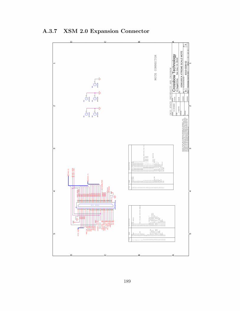
A.3.7 XSM 2.0 Expansion Connector

5 5

4 4

3 3

2 2

1 1

DD

CC

BB

AA

PW

2IN

T2

AD

C7

PW

5

TH

RU

1

INT

3

AD

C6

AD

C2

PW

0

AD

C0

TH

RU

2

PW

6

AD

C1

UA

RT

_TX

D0

PW

1

TH

RU

3

INT

0

AD

C4

INT

1

PW

4P

W3

AD

C3

UA

RT

_RX

D0

PW

7

AD

C5

VC

C

VC

C

LED

1 SP

I_S

CK

I2C

_C

LK

MA

G_S

R

PW

M1A

RS

TN

PW

[0..

7]

WR

UA

RT

_TX

D0

US

AR

T1_

TX

D

US

AR

T1_

CLK

LED

2

PW

M0

AC

-

INT

[0..

3]

RD

TH

ER

M_P

WR

US

AR

T1_

RX

D

LED

3

ALE I2

C_

DA

TA

AC

+

PW

M1B

AD

C[0

..7

]

UA

RT

_RX

D0

Titl

e

Siz

eD

ocu

men

t N

um

ber

Re

v

Da

te:

Sh

eet

of

EX

CE

PT

AS

MA

Y B

E O

TH

ER

WIS

E P

RO

VID

ED

BY

CO

NT

RA

CT

, T

HIS

DR

AW

ING

OR

SP

EC

IFIC

AT

ION

IS

TH

E P

RO

PR

IET

AR

Y P

RO

PE

RT

Y O

FC

RO

SS

BO

W T

EC

HN

OLO

GY

IN

C.

IT

IS

IS

SU

ED

IN

ST

RIC

T C

ON

FID

EN

CE

AN

D S

HA

LL

NO

T B

E R

EP

RO

DU

CE

D O

R C

OP

IED

OR

US

ED

(P

AR

TIA

LLY

OR

WH

OL

LY

) IN

AN

Y M

AN

NE

R W

ITH

OU

T P

RIO

R E

XP

RE

SS

WR

ITT

EN

AU

TH

OR

IZA

TIO

N O

F C

RO

SS

BO

W T

EC

HN

OLO

GY

IN

C.

DA

TE

DW

N

CH

K

AP

RV

D

AP

RV

D63

10-0

336-

02A

XS

M10

0CA

XT

RE

ME

SC

ALE

MO

TE

Cro

ssbo

w T

echn

olog

y41

Dag

gett

Driv

eS

an J

ose,

CA

. 951

34

B5

8W

ed

nes

day

, Ju

ne

30

, 2

00

4

X

XX

/XX

/XX

5-14

-04

XX

/XX

/XX

P.

DU

TT

A

X

M.

GR

IMM

ER

5-14

-04

PIN

NAME

DESCRIPTION

1 2 3 4 5 6 7 8 9 10

11

12

13

14

15

16

17

18

19

20

21

22

23

24

25

26

GND

VSNSR

INT3

INT2

INT1

INT0

BAT_MON

LED3

LED2

LED1

RD

WR

ALE

PW7

USART1_CLK

PROG_MOSI

PROG_MISO

SPI_SCK

USART1_RXD

USART1_TXD

I2C_CLK

I2C_DATA

PWM0

PWM1A

AC+

AC-

GROUND

SENSOR SUPPLY

GPIO

GPIO

GPIO

GPIO

BATTERY VOLTAGE MONITOR ENABLE

LED3

LED2

LED1

GPIO

GPIO

GPIO

POWER CONTROL 7

USART1 CLOCK

SERIAL PROGRAM MOSI

SERIAL PROGRAM MISO

SPI SERIAL CLOCK

USART1 RX DATA

USART1 TX DATA

I2C BUS CLOCK

I2C BUS DATA

GPIO/PWM0

GPIO/PWM1A

GPIO/AC+

GPIO/AC-

UART_RXD0

UART_TXD0

PW0

PW1

PW2

PW3

PW4

PW5

PW6

ADC7

ADC6

ADC5

ADC4

ADC3

ADC2

ADC1

ADC0

THERM_PWR

THRU1

THRU2

THRU3

RSTN

PWM1B

VCC

GND

NAME

27

28

29

30

31

32

33

34

35

36

37

38

39

40

41

42

43

44

45

46

47

48

49

50

51

PIN

DESCRIPTION

UART_0 RECEIVE

UART_0 TRANSMIT

POWER CONTROL 0

POWER CONTROL 1

POWER CONTROL 2

POWER CONTROL 3

POWER CONTROL 4

POWER CONTROL 5

POWER CONTROL 6

ADC INPUT 7 - BATTERY MONITOR/JTAG TDI

ADC INPUT 6 / JTAG TDO

ADC INPUT 5 / JTAG TMS

ADC INPUT 4 / JTAG TCK

ADC INPUT 3

ADC INPUT 2

ADC INPUT 1

ADC INPUT 0 / RSSI MONITOR

TEMP SENSOR ENABLE

THRU CONNECT 1

THRU CONNECT 2

THRU CONNECT3

RESET (NEG)

GPIO/PWM1B

DIGITAL SUPPLY

GROUND

MOTE CONNECTOR

PROG_MOSI

PROG_MISO

OHIO STATE UNIVERSITY AND CROSSBOW

HIROSE PLUG

J5

DF

9-5

1P-1

V(5

4)

1 2 3 4 5 6 7 8 9 10 11 12 13 14 15 16 17 18 19 20 21 22 23 24 25 26

27 28 29 30 31 32 33 34 35 36 37 38 39 40 41 42 43 44 45 46 47 48 49 50 51

M5

MT

G12

8

11

M3

MT

G12

8

11

M4

MT

G12

8

11

M1

MT

G12

8

11

M2

MT

G12

8

11

189

A.3.8 XSM 2.0 Microcontroller and Memory Subsystem

5 5

4 4

3 3

2 2

1 1

DD

CC

BB

AA

FL

AS

H_

CS

SE

RIA

L_

ID

PW

7P

W6

PW

5P

W4

PW

3P

W2

PW

1P

W0

US

AR

T1_

RX

DU

SA

RT

1_C

LKU

SA

RT

1_T

XD

UA

RT

_TX

D0

US

AR

T1_

RX

D

LED

3

FL

AS

H_

CS

FL

AS

H_

CS

SP

I_M

OS

IA

DC

3

AD

C5

AD

C4

AD

C0

AD

C6

AD

C2

AD

C7

AD

C1

INT

1IN

T2

INT

3

INT

0

INT

[0..

3]

LED

1

LED

2

SE

RIA

L_

ID

PW

M1A

PW

M1C

INT

0

I2C

_C

LK

I2C

_D

AT

A ALE

ALE

RS

TN

VC

C

VC

C

VC

C

VC

CV

CC

VC

C

VC

C

VS

NS

R

VC

C

VC

C

VC

C

VC

C

PC

LKP

DA

TA

LED

3LE

D2

LED

1

MA

G_S

RC

HP

_O

UT

TH

ER

M_P

WR

PW

[0..

7]

SP

I_S

CK

PW

M0

PW

M1A

PW

M1B

RS

TN

INT

[0..

3]

UA

RT

_RX

D0

UA

RT

_TX

D0

AC

-

AD

C[0

..7

]

WR

RD

ALE

SP

I_M

ISO

I2C

_C

LK

I2C

_D

AT

AU

SA

RT

1_R

XD

US

AR

T1_

TX

DP

ALE

US

AR

T1_

CLK

AC

+

PW

M1C

SE

RIA

L_

ID

I2C

_D

AT

A1

I2C

_C

LK

1

I2C

_C

LK

0I2

C_

DA

TA

0

Titl

e

Siz

eD

ocu

men

t N

um

ber

Re

v

Da

te:

Sh

eet

of

EX

CE

PT

AS

MA

Y B

E O

TH

ER

WIS

E P

RO

VID

ED

BY

CO

NT

RA

CT

, T

HIS

DR

AW

ING

OR

SP

EC

IFIC

AT

ION

IS

TH

E P

RO

PR

IET

AR

Y P

RO

PE

RT

Y O

FC

RO

SS

BO

W T

EC

HN

OLO

GY

IN

C.

IT

IS

IS

SU

ED

IN

ST

RIC

T C

ON

FID

EN

CE

AN

D S

HA

LL

NO

T B

E R

EP

RO

DU

CE

D O

R C

OP

IED

OR

US

ED

(P

AR

TIA

LLY

OR

WH

OL

LY

) IN

AN

Y M

AN

NE

R W

ITH

OU

T P

RIO

R E

XP

RE

SS

WR

ITT

EN

AU

TH

OR

IZA

TIO

N O

F C

RO

SS

BO

W T

EC

HN

OLO

GY

IN

C.

DA

TE

DW

N

CH

K

AP

RV

D

AP

RV

D63

10-0

336-

02A

XS

M10

0CA

XT

RE

ME

SC

ALE

MO

TE

Cro

ssbo

w T

echn

olog

y41

Dag

gett

Driv

eS

an J

ose,

CA

. 951

34

B6

8W

ed

nes

day

, Ju

ne

30

, 2

00

4

X

XX

/XX

/XX

5-14

-04

XX

/XX

/XX

P.

DU

TT

A

X

M.

GR

IMM

ER

5-14

-04

CPU/FLASH/SERIAL ID

OHIO STATE UNIVERSITY AND CROSSBOW

NO STUFF

NO STUFF

R68

100K

C46

1000

pF

U12

DS

2401

P

DQ

2

D8

YE

LL

OW

12

C43

.1u

F

C47

1000

pF

C39

.01

uF

C44

.1u

F

1 0

U44 N

C7

SB

3157

31

65

4

R36

10K

R34

1M

D4

GR

EE

N

12

R31

10K

R90

100K

C50

12pF

C40

.01

uF

D7

GR

EE

N

12

C38

.01

uF

C45

.1u

F

C73

0.1

uF

R32

1M

D3

RE

D

12

R38

470

Y2

7.3

728

MH

Z

X2

2

X2

3X

14

X1

1

C36

10uF

6.3

V

Y3

32

.76

8K

HZ21

34

C48

1000

pF

R40

470

R91

100K

U10

AT

ME

GA

128L

PA

0/A

D0

51

PA

1/A

D1

50

PA

2/A

D2

49

PA

3/A

D3

48

PA

4/A

D4

47

PA

5/A

D5

46

PA

6/A

D6

45

PA

7/A

D7

44

PB

0/S

S10

PB

1/S

CK

11

PB

2/M

OS

I12

PB

3/M

ISO

13

PB

4/O

C0

14

PB

5/O

C1A

15

PB

6/O

C1B

16

PB

7/O

C1C

17

PC

0/A

835

PC

1/A

936

PC

2/A

1037

PC

3/A

1138

PC

4/A

1239

PC

5/A

1340

PC

6/A

1441

PC

7/A

1542

PD

0/IN

T0

25

PD

1/IN

T1

26

PD

2/R

XD

127

PD

3/T

XD

128

PD

4/IC

129

PD

5/X

CK

130

PD

6/T

131

PD

7/T

232

PE

0/R

XD

02

PE

1/T

XD

03

PE

2/X

CK

04

PE

3/O

C3A

5

PE

4/O

C3B

6

PE

5/O

C3C

7

PE

6/T

38

PE

7/IC

39

PF

0/A

DC

061

PF

1/A

DC

160

PF

2/A

DC

259

PF

3/A

DC

358

PF

4/T

CK

57

PF

5/T

MS

56

PF

6/T

DO

55

PF

7/T

DI

54

AVCC64

AREF62

PE

N1

RST20XTAL1 24

XTAL2 23

PG

0/W

R33

PG

1/R

D34

PG

2/A

LE43

PG3/TOSC2 18PG4/TOSC1 19

1 0

U45

NC

7S

B31

57

31

65

4C

5112

pF

C37

.01

uF

D6

RE

D

12

D5

YE

LL

OW

12

C41

.01

uF

SW

3

PB

SP

ST

RA

12

34

R9

100K

R67

10.0

K

R30

470

R37

4.7K

SW

2

PB

SP

ST

12

53 4

C49

1000

pF

U11

AT

45D

B04

1

SI

1

SC

K2

RS

T3

CS

4W

P5

SO

8

R35

10K

R33

0 O

HM

C42

.01

uF

R39

470

R10

4

10K

190

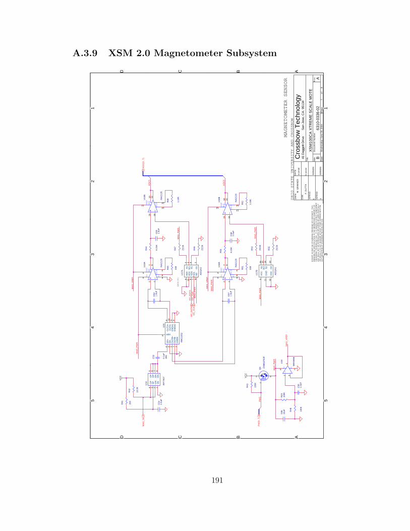
A.3.9 XSM 2.0 Magnetometer Subsystem

5 5

4 4

3 3

2 2

1 1

DD

CC

BB

AA

PW

5

MA

G_P

WR

MA

G_P

WR M

AG

_VR

EF

MA

G_P

WR

I2C

_D

AT

A

AD

C6

MA

G_P

WR

MA

G_V

RE

F

MA

G_V

RE

F

AD

C5

MA

G_P

WR

I2C

_C

LK

MA

G_P

WR

MA

G_P

WR

VC

C VC

C

MA

G_S

R

PW

[0..

7]

I2C

_C

LK

1I2

C_

DA

TA

1

AD

C[0

..7

]

Titl

e

Siz

eD

ocu

men

t N

um

ber

Re

v

Da

te:

Sh

eet

of

EX

CE

PT

AS

MA

Y B

E O

TH

ER

WIS

E P

RO

VID

ED

BY

CO

NT

RA

CT

, T

HIS

DR

AW

ING

OR

SP

EC

IFIC

AT

ION

IS

TH

E P

RO

PR

IET

AR

Y P

RO

PE

RT

Y O

FC

RO

SS

BO

W T

EC

HN

OLO

GY

IN

C.

IT

IS

IS

SU

ED

IN

ST

RIC

T C

ON

FID

EN

CE

AN

D S

HA

LL

NO

T B

E R

EP

RO

DU

CE

D O

R C

OP

IED

OR

US

ED

(P

AR

TIA

LLY

OR

WH

OL

LY

) IN

AN

Y M

AN

NE

R W

ITH

OU

T P

RIO

R E

XP

RE

SS

WR

ITT

EN

AU

TH

OR

IZA

TIO

N O

F C

RO

SS

BO

W T

EC

HN

OLO

GY

IN

C.

DA

TE

DW

N

CH

K

AP

RV

D

AP

RV

D63

10-0

336-

02A

XS

M10

0CA

XT

RE

ME

SC

ALE

MO

TE

Cro

ssbo

w T

echn

olog

y41

Dag

gett

Driv

eS

an J

ose,

CA

. 951

34

B7

8W

ed

nes

day

, Ju

ne

30

, 2

00

4

X

XX

/XX

/XX

5-14

-04

XX

/XX

/XX

P.

DU

TT

A

X

M.

GR

IMM

ER

5-14

-04

MAGNETOMETER SENSOR

OHIO STATE UNIVERSITY AND CROSSBOW

ADDR[00]

R51

330

U15

HM

C10

52

GN

DB

1

OU

TB

+2

GN

DA

13

OU

TA

+4

VBR5

SR

+6

OU

TB

-7

SR

-8

GN

DA

29

OU

TA

-10

C58

1.0

uF

U17

A

AD

5242A

12

W1

3

B1

4

SD

6S

CL

7S

DA

8

AD

09

AD

110

O1

1

C56

1.0

uF

C55

1.0

uF

R55

25.5

K

R23

100K

C52

1.0

uF

R43

100K

GAIN

SNS

VREFU

13B

INA

21

26

15 16

13

14

1110

12

GAIN

V+

V-

SNS

VREF

U18

A

INA

21

26

2 1

4

3

9 8

67

5

R52

1.10

K

R49

25.5

K

U14

IRF

75

07

SN

1G

N2

SP

3G

P4

DP

5

DP

6

DN

7

DN

8

R44

8.2

5K

U17

B

AD

5242A

216

W2

15

B2

14

O2

13V

SS

12

VC

C5

GN

D11

R41

200

R48

100K

R47

25.5

K

C53

0.1

uF

25V

R53

25.5

K

C57

1.0

uF

C54

1.0

uF

R50

8.2

5K

Q3 ZX

M61

P03

F

1

32GAIN

V+

V-

SNS

VREF

U13

A

INA

21

26

2 1

4

3

9 8

67

5

C65

10uF

R45

330

+ -

V+

V-

U16

MA

X44

66

1 34

5 2

GAIN

SNS

VREF

U18

B

INA

21

26

15 16

13

14

1110

12

R46

1.10

K

R42

10.0

K

191

A.3.10 XSM 2.0 Passive Infrared Subsystem

5 5

4 4

3 3

2 2

1 1

DD

CC

BB

AA

PIR

_P

WR

PIR

_P

WR

PIR

_P

WR

PIR

_P

WR

INT

2

AD

C7

PIR

_P

WR

PW

6

PIR

_P

WR

PIR

_P

WR

PIR

_P

WR

PIR

_P

WR

PIR

_P

WR

VC

C

AD

C[0

..7

]

I2C

_D

AT

A1

INT

[0..

3]

I2C

_C

LK

1

PW

[0..

7]

PW

M0

PW

M1A

AC

+

AC

-

Titl

e

Siz

eD

ocu

men

t N

um

ber

Re

v

Da

te:

Sh

eet

of

EX

CE

PT

AS

MA

Y B

E O

TH

ER

WIS

E P

RO

VID

ED

BY

CO

NT

RA

CT

, T

HIS

DR

AW

ING

OR

SP

EC

IFIC

AT

ION

IS

TH

E P

RO

PR

IET

AR

Y P

RO

PE

RT

Y O

FC

RO

SS

BO

W T

EC

HN

OLO

GY

IN

C.

IT

IS

IS

SU

ED

IN

ST

RIC

T C

ON

FID

EN

CE

AN

D S

HA

LL

NO

T B

E R

EP

RO

DU

CE

D O

R C

OP

IED

OR

US

ED

(P

AR

TIA

LLY

OR

WH

OL

LY

) IN

AN

Y M

AN

NE

R W

ITH

OU

T P

RIO

R E

XP

RE

SS

WR

ITT

EN

AU

TH

OR

IZA

TIO

N O

F C

RO

SS

BO

W T

EC

HN

OLO

GY

IN

C.

DA

TE

DW

N

CH

K

AP

RV

D

AP

RV

D63

10-0

336-

02A

XS

M10

0CA

XT

RE

ME

SC

ALE

MO

TE

Cro

ssbo

w T

echn

olog

y41

Dag

gett

Driv

eS

an J

ose,

CA

. 951

34

B8

8W

ed

nes

day

, Ju

ne

30

, 2

00

4

X

XX

/XX

/XX

5-14

-04

XX

/XX

/XX

P.

DU

TT

A

X

M.

GR

IMM

ER

5-14

-04

PIR SENSOR

OHIO STATE UNIVERSITY AND CROSSBOW

ADDR[01]

R83

1.00

M

R59

47.5

K

C61

2.2

UF

C90

47uF

+ -

V+

V-

U34

MA

X44

66

1 34

5 2

R79

4.7K

V+

V-

+ -

U22

LMC

7225

5

31

2

4

R87

47.5

KV+

V-

+ -

U40

LMC

7215

5

31

2

4

R65

100K

V+

V-

+ -

U43

LMC

7215

5

31

2

4

R13

100K

R73

100K

R89

1.00

M

PIR

D S

U26

LH

I87

8

321

+ -

V+

V-

U36

MA

X44

66

1 34

5 2

C92

47uF

C70

1000

pF

C82

2.2

UF

C83

1000

pF

C63

47uF

+ -

V+

V-

U24

MA

X44

66

1 34

5 2

C72

10uF

U29

B

AD

5242A

216

W2

15

B2

14

O2

13V

SS

12

VC

C5

GN

D11

C62

0.0

15uF

R80

4.7K

C89

2.2

UF

R56

100K

C68

47uF

+ -

V+

V-

U35

MA

X44

66

1 34

5 2

V+

V-

+ -

U41

LMC

7215

5

31

2

4

R14

100K

PIR

D S

U27

LH

I87

8

321

C85

0.0

1uF

R60

1.00

M

C66

.1u

F

Q4 ZX

M61

P03

F

1

32

C93

0.0

1uF

C87

1000

pF

R84

47.5

K

R58

4.7K

R88

10.0

K

C86

2.2

UF

C64

0.0

1uF

R10

5

25.5

K

R82

10.0

K

C97

10uF

R71

100K

R62

1.00

M

C91

1000

pF

PIR

D S

U19

LH

I87

8

321

U29

A

AD

5242A

12

W1

3

B1

4

SD

6S

CL

7S

DA

8

AD

09

AD

110

O1

1

R85

10.0

K

V+

V-

+ -

U28

LMC

7225

5

31

2

4

V+

V-

+ -

U42

LMC

7215

5

31

2

4

R86

1.00

M

R77

4.7K

C67

1000

pF

C88

0.0

1uF

+ -

V+

V-

U23

MA

X44

66

1 34

5 2

R10

6

25.5

K

R81

47.5

K

R72

100K

C84

47uF

PIR

D S

U25

LH

I87

8

321

R61

10.0

K

C71

10uF C

98

10uF

192

APPENDIX B

CIRCUIT SIMULATIONS

B.1 Acoustic

Microphone Bandpass Filter (Cascaded Sallen-Key LPF and HPF) Circuit Frequency Response (at 4kHz)

* OPAMP V+ V- Vo Gnd

.SUBCKT OPAMP 1 2 4 5

R1 2 1 1e6

E1 3 5 2 1 1e4

R0 3 4 50

.ENDS OPAMP

* LPF Vi Gnd Vo

.SUBCKT LPF 1 10 6

Cin 1 2 1e-6

C1 4 10 .01e-6

C2 6 3 .022e-6

R1 2 3 2680

R2 3 4 2680

R3 6 5 100e3

X1 5 4 6 10 OPAMP

.ENDS LPF

* HPF Vi Gnd Vo

.SUBCKT HPF 1 10 5

C1 1 2 1e-7

C2 2 3 1e-7

R1 3 10 281

R2 5 2 562

R3 5 4 100e3

X1 4 3 5 10 OPAMP

.ENDS HPF

X1 1 0 2 LPF

X2 2 0 3 HPF

V1 1 0 AC 1

.AC DEC 300 100 1000000

.PROBE

.END

193

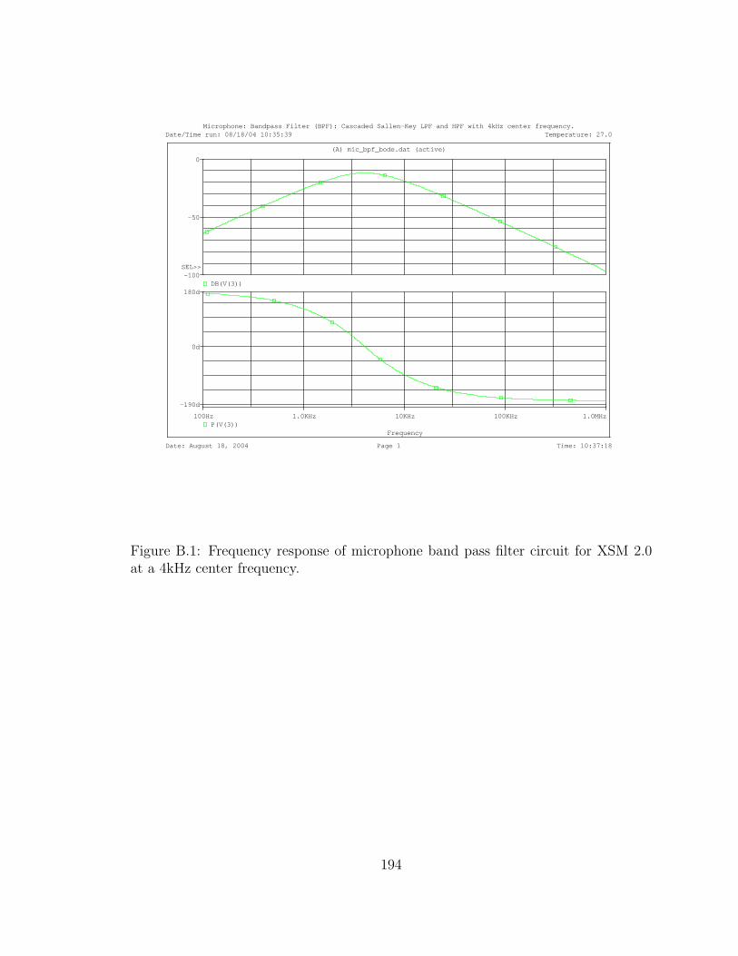
Date/Time run: 08/18/04 10:35:39Microphone: Bandpass Filter (BPF): Cascaded Sallen-Key LPF and HPF with 4kHz center frequency.

Temperature: 27.0

Date: August 18, 2004 Page 1 Time: 10:37:18

(A) mic_bpf_bode.dat (active)

Frequency

100Hz 1.0KHz 10KHz 100KHz 1.0MHzP(V(3))

-190d

0d

180dDB(V(3))

-100

-50

0

SEL>>

Figure B.1: Frequency response of microphone band pass filter circuit for XSM 2.0at a 4kHz center frequency.

194

B.2 Passive Infrared

PIR Signal Conditioning Circuit Frequency Response

* OPAMP: V- (1), V+ (2), Vout(4), Gnd (5)

.SUBCKT OPAMP 1 2 4 5

R1 2 1 1e6

E1 3 5 2 1 1e4

R0 3 4 50

.ENDS OPAMP

X1 3 1 2 0 OPAMP

C1 2 3 .01e-6

R1 2 3 1e6

C2 4 0 47e-6

R2 3 4 10e3

V1 1 0 AC 1mV

C3 2 5 2.2e-6

R3 5 8 4.7e3

X2 8 6 7 0 OPAMP

C4 7 8 .015e-6

R4 7 8 1e6

V2 100 0 DC 3

V3 0 101 DC 3

Rp 100 6 25e3

Rn 101 6 25e3

.AC DEC 100 0.001 10000

.PROBE

.END

195

Date/Time run: 07/03/04 02:31:03PIR Signal Conditioning Circuit Frequency Response

Temperature: 27.0

Date: July 03, 2004 Page 1 Time: 02:31:13

(A) pir_bpf_bode.dat (active)

Frequency

1.0mHz 10mHz 100mHz 1.0Hz 10Hz 100Hz 1.0KHz 10KHzP(V(7))

-400d

-200d

0ddB(V(7)/V(1))

-40

0

40

80

SEL>>

Figure B.2: Frequency response of PIR signal conditioning circuit for XSM 2.0.

196

APPENDIX C

PACKAGING CONCEPTS

Sensor nodes for intrusion detection may experience diverse and hostile environ-

ments with wind, rain, snow, flood, heat, cold, terrain, and canopy. The sensor

packaging is responsible for protecting the delicate electronics from these elements.

In addition, the packaging can affect the sensing and communications processes either

positively or negatively. We present several packaging concepts that were considered

for the XSM as well an enclosure design that was selected for an earlier radar sensor

node:

• Capsule: A self-righting enclosure for the radar sensor.

• Hockey Puck: A compact enclosure concept for the XSM.

• Cone: A partially self-righting enclosure concept for the XSM.

• COTS (1): A modified COTS enclosure concept for the XSM.

• COTS (2): An improved version of COTS (1) enclosure for the XSM.

197

C.1 Capsule

Figure C.1: Capsule enclosure.

The capsule-shaped enclosure is smooth and provides a self-righting capability

and minimizes wind-resistance. The enclosure body is clear to allow sunlight to illu-

minate a solar cell mounted inside. Unfortunately, this has the side effect of heating

the electronics to a level at which they intermittently fail. The sensor electronics are

mounted on a frame that is attached to the enclosure shell using a single gimbal mech-

anism. The gimbal is free to rotate along the long axis of the enclosure. The frame is

asymmetrically weighted in favor of the side with batteries so that the batteries are

on the bottom and a solar cell is on top. The gimbal mechanism, when coupled with

the rotational degree of freedom of the cylindrical enclosure, increases the likelihood

198

that the radar and radio antennas plane will be perpendicular to the ground and the

solar cell will be pointing toward the sky, helping to increase the node’s sensing range,

communications range, and lifetime.

199

C.2 Hockey Puck

2.20

1.80

SolidWorks Student LicenseAcademic Use Only Figure C.2: Hockey puck enclosure.

The hockey puck-shaped enclosure shown in Figure C.2 consists of a cover, body,

and base. The base is a mostly solid cylindrical plastic piece which increases the mass

near the bottom of the package, lowering the overall center-of-gravity, and reducing

the likelihood of the package tipping over. The base has a square-shaped cavity that

can house batteries. A second cylindrically-shaped cavity extends upward from the

battery compartment and acts as a friction-fit holder for the sounder. A smaller

cylindrical cavity extends from the top of the sounder compartment and emerges as

a hole on the top of the base. This small cavity serves as an acoustic waveguide,

channeling energy from the sounder to the environment. A similar cavity and hole

exists on the body to expose the microphone to the environment. The circular top face

200

of the base has a centered and recessed circular ring. The purpose of the recessed ring

is to aid with self-guided assembly when mating with the body which has matching

polarized holes and countersunk bosses. The body is manufactured either from an

infrared-transparent plastic or has cutouts for four passive infrared sensors. The XSM

is mounted upside down in this enclosure and the PIR reflectors protrude downward

into the four pie-slice shaped cavities.

201

C.3 Cone

SolidWorks Student LicenseAcademic Use OnlyFigure C.3: Cone enclosure, Source: Crossbow Technology.

The cone-shaped enclosure was motivated by the desire for a self-righting capabil-

ity. With such a feature, the a node could be “tossed down” much like a traffic cone

and we would be reasonably confident that it would land right-side-up and that the

magnetometers would be level. While the wide base helps to reduce the likelihood of

the cone tipping over, we would have had to add a significant amount of weight to

202

the cone’s base to ensure the self-righting capability across the spectrum of possible

laydowns.

An interesting aspect of this design is a “hanging pendulum” circuit board which

is suspended by the antenna. The figure shows the The antenna itself is attached to

the apex of the cone. However, the proposed “swivel” of the circuit board would only

have been ±10 deg to ±15 deg which would correspond to a change of less than 2-4 %

in the projection of the magnetic field onto the tilted circuit board. In other words,

for inclines not exceeding ±15 deg, very little would be gained from this feature.

203

C.4 COTS Box A

Figure C.4: Simple COTS enclosure. Source: Crossbow Technology.

The commerically-available box-shaped enclosure was motivated by a desire to

reduce cost and leverage standard products.

204

C.5 COTS Box B

Figure C.5: Heavily-modified COTS enclosure. Source: Crossbow Technology.

A variation on COTS Box A, this design inverted the circuit board, added acoustic

holes, and increased the PIR cutouts. The circuit board was inverted for two reasons.

First, by inverting the circuit board, we were able to maximize the separation between

the magnetometer and batteries. Since batteries contain magnetic materials, their

205

presence near a magnetometer tends to diminish the sensor’s sensitivity. Second,

inverting the board increased the height of the antenna by about one inch. Low-lying

antennas tend to experience increased ground absorbtion and reduced range, so by

increasing the separation between the antenna and ground, we expect to improve the

node’s transmission range.

Figure C.6: Heavily-modified COTS enclosure (transparent). Source: Crossbow Tech-nology.

206

APPENDIX D

EXPERIMENTAL DATA

D.1 Magnetometer

Preliminary experiments indicated that a number of variables affect the magni-

tude and direction of the magnetic field at a test point as a result of a ferromagnetic

object’s passage nearby. These variables include an object’s length, mass, magne-

tization, permeability, distance from the test point, orientation with respect to the

point, orientation with respect to Earth’s magnetic field, and presence of nearby fer-

romagnetic materials. The following experiments are designed to provide empirical

evidence to support a subset of the variables contemplated in the analytical model.

The experiments also provide training data for filtering, detection, classification, and

estimation algorithms.

D.1.1 Procedural Considerations

A number of procedural considerations were discovered, some in the literature,

and some experientially, that are summarized here. Following these recommendations

helps reduce the sources of noise during the data collection process and the sources

of confusion during the subsequent data analysis process.

207

Nomenclature: The term “experimental setup” or “configuration” is used to in-

dicate a static configuration of sensors. The term “experiment” refers to a

dynamic configuration used to test a hypothesis. Experiments are numbered

using Arabic numerals. The term “subexperiment” is used indicate a variation

in one or more experimental parameters like velocity or orientation but without

changing the hypothesis under test. Subexperiments are denoted by appending

a Roman capital letter to experiment identifier. The term “trial” indicates a

single execution of a given experiment or subexperiment. Trials are numbered

using Arabic numerals appended to subexperiment identifiers. The symbol B

is used to denote the magnitude of a magnetic field and Bx, By, and Bz denote

the x, y, and z components of B. The symbols vX and τX represent the target’s

velocity and a time offset for the subexperiment, respectively.

Orientation: A consistent orientation of the sensors with respect to the ambient

magnetic field is important for training data. In earlier experiments, the sen-

sitive axes A and B of the magnetometer (and x and y, respectively, for the

nomenclature used here), were oriented west and south in one setup, and north

and west in another setup. The data that was collected in those experiments

was the sum the x and y axis values, essentially resulting in an attempt to

compare Bx + By with Bx − By. The lesson is that sensor orientation matters

and that attention should be paid to a magnetometer’s sensitive axis. For the

following experiments, the sensitive axes are pointed west and south.

Orthogonality: The real problem with orientation was that the x and y components

of the magnetic field were not reported separately. This shortcoming occurred

208

due to an initially poor understanding of the theoretical model. Filtering, arith-

metical, statistical and other operations on the raw x and y data may be more

meaningful than operations on combined data streams.

Placement: It is best to avoid placing the sensors near metal objects like light poles

as these objects are likely to distort the ambient magnetic field. A compass can

be used to verify that the x and y components of the ambient magnetic field

are constant throughout the sensor test bed.

Clock Synchronization: Earlier experiments demonstrated very low clock drift

(less than 0.03%) over a period spanning more than 30 minutes and across

six separate sensors. It is unclear whether this difference is due to true clock

drift or the loss of data samples during the downloading process. Regardless,

a reasonable conclusion appears to be that in experiments lasting minutes to

hours, initial clock synchronization is sufficient and no explicit ongoing clock

synchronization is necessary over the duration of the experiment.

Personnel: The personnel carrying out these experiments should avoid wearing steel

toed shoes, metal belt buckles, and other ferromagnetic materials near the sen-

sors in order to avoid generating spurious signals.

Site Description: It is useful to capture location, weather, date, time-of-day, a site

picture, and ambient magnetic field at the sensor test bed. For the last of these

items, the National Geophysical Data Center, a part of the National Oceanic and

209

Atmospheric Association, which is itself a part of the U.S. Department of Com-

merce, hosts an online implementation of the International Geomagnetic Refer-

ence Field, a model that can compute the expected magnetic field at any point

on the Earth’s surface: http://www.ngdc.noaa.gov/IAGA/wg8/wg8.html.

D.1.2 Experimental Setup

Honeywell HMC-1002 2-axis magnetometers [66] were used as the magnetic sensor

and Mica Motes developed at Berkeley were used for the experimental platform [41]

in these experiments. There were several experimental setups or configurations used

in the experiments.

L-Setup

The L-Setup consisted of six 2-axis sensors sampling at frequency fs of 20Hz. A

pair of sensors were placed at each of the three vertices of a 24ft by 32ft L-shaped

region. If the pair of sensors located at the knee of the L is defined as the origin of a

coordinate plane with the positive y-axis pointing North, then the sensors are located

at (0,0), (24,0), and (32,0). The overall size of the sensor test bed is 40ft by 40ft and

the visible grid is on 4ft by 4ft centers.

X-Setup

Setup X consisted of five 2-axis sensors sampling at frequency fs of 20Hz. Four

of the sensors are placed at the vertices of a 16ft by 16ft square and the fifth sensor

is placed at the center of the square, in an X-shape, as shown in Figure D.1 (not to

scale). If the fifth and centrally-located sensor is defined as the origin of a coordinate

plane with the positive y-axis pointing North, then the sensors are located at (0,0),

210

(-20,-20)

(20,20)

(20,-20)

(-20,20)

(0,0)

(8,8) (-8,8)

(-8,-8) (8,-8)

N

Figure D.1: Experimental Setup.

(8,8), (-8,8), (-8,-8), and (8,-8). The overall size of the sensor test bed is 40ft by 40ft

and the visible grid is on 4ft by 4ft centers.

D.1.3 Experiments

This section describes the specific experiments that were carried out. The experi-

ments were designed to test noise statistics and the relationship between the strength

of the magnetic field at a test point as function of a target’s velocity, distance from

the test point, orientation with respect to the point, and orientation with respect to

211

Earth’s magnetic field. Due to limited time and resources, some of the contemplated

variables were not tested in isolation. Specifically, length, mass, magnetization, and

permeability were not tested in independently. These variables are coupled for most

of the easily available targets, so the target’s length and mass are noted, and its

magnetization and permeability are ignored.

Control

The purpose of the control was to capture the ambient or background noise void

of any external stimuli. Control data was captured by letting the sensors collect data

prior to starting any of the experiments. The experiments indicated that the power

spectral density of the background noise varied significantly. This majority of this

variability appears as gaussian random noise. However, non-random sources of noise

appear to be present as well.

Noise Floor

The noise floor of a measurment device is the measured noise with the device’s

inputs grounded. The noise characteristics of the Honeywell sensor is availabled in

[66] but the noise characteristics of the entire measurement system including the

two-stage amplifier and analog-to-digital converter are not known. The noise floor

consists of a number of components including 1/f noise and wideband noise. While

it is not possible to directly “ground” the magnetometer inputs, the sensor can be

placed inside a Faraday cage for the purpose of taking noise floor measurements. A

poor man’s Faraday cage was constructed from a sheet of aluminum foil as follows.

First, the sensor was wrapped with a non-conducting plastic material to prevent

short-circuiting. Then, the plastic foil encased sensor was wrapped in a sheet of

212

aluminum foil. The aluminum foil created a closed conducting surface. Finally, both

the aluminum and plastic foils were removed, concluding the experiment. The sensors

collected samples during this entire process.

Preliminary

The preliminary experiments were designed to familiarize the

Velocity

The purpose of this experiment was to determine the relationship between the

target’s velocity and magnetic signature. The hypothesis under test was that different

speeds will stretch and shrink the signal temporally, for slower and faster speeds,

respectively. The data indicates that reversing the direction of travel will cause the

sign of the signal to be reversed, relative to a bias, if present. Six subexperiments are

used to test the hypothesis. In this experiment, the target’s direction and speed of

travel are varied. The experiment is depicted graphically in Figure D.2. The double-

ended red arrow represents the target’s motion. The specific variations to the target’s

speed and direction are enumerated below. Subexperiment A

1. Velocity: vA =5mph (7.33fps); west → east

2. Trajectory (fps): x(t) = vA(t− τA); y(t) = −16

3. Target: 1999 Honda Accord

4. Trials: 3

Subexperiment B

1. Velocity: vB =10mph (14.66fps); west → east

213

(-20,-20)

(20,20)

(20,-20)

(-20,20)

(0,0)

(8,8) (-8,8)

(-8,-8) (8,-8)

Figure D.2: Velocity Experiment.

214

2. Trajectory (fps): x(t) = vB(t− τB); y(t) = −16

3. Target: 1999 Honda Accord

4. Trials: 3

Subexperiment C

1. Velocity: vC =15mph (22fps); west → east

2. Trajectory (fps): x(t) = vC(t− τC); y(t) = −16

3. Target: 1999 Honda Accord

4. Trials: 3

Subexperiment D

1. Velocity: vD =5mph (7.33fps); east → west

2. Trajectory (fps): x(t) = −vD(t− τD); y(t) = −16

3. Target: 1999 Honda Accord

4. Trials: 3

Subexperiment E

1. Velocity: vE =10mph (14.66fps); east → west

2. Trajectory (fps): x(t) = −vE(t− τE); y(t) = −16

3. Target: 1999 Honda Accord

4. Trials: 3

215

Subexperiment F

1. Velocity: vF =15mph (22fps); east → west

2. Trajectory (fps): x(t) = −vF (t− τF ); y(t) = −16

3. Target: 1999 Honda Accord

4. Trials: 3

Distance

This experiment attempts to determine the relationship between the target’s dis-

tance from the sensor and the strength of the detected magnetic field. The hypothesis

under test was that the magnetic field strength drops off in a 1/r2 fashion. Ten subex-

periments are used to test the hypothesis. In this experiment, the target’s direction

and distance from sensor are varied. The experiment is depicted graphically in Fig-

ure D.3. There are two orthogonal sets of single-ended red arrows representing the

target’s motion. The specific variations to the target’s distance and direction are

enumerated below.

Subexperiment A

1. Velocity: vA =10mph (14.66fps); west → east

2. Trajectory (fps): x(t) = vA(t− τA); y(t) = −16

3. Target: 1999 Honda Accord

4. Trials: 3

Subexperiment B

216

(-20,-20)

(20,20)

(20,-20)

(-20,20)

(0,0)

(8,8) (-8,8)

(-8,-8) (8,-8)

Figure D.3: Distance Experiment.

217

1. Velocity: vB =10mph (14.66fps); west → east

2. Trajectory (fps): x(t) = vB(t− τB); y(t) = −8

3. Target: 1999 Honda Accord

4. Trials: 3

Subexperiment C

1. Velocity: vC =10mph (14.66fps); west → east

2. Trajectory (fps): x(t) = vC(t− τC); y(t) = 0

3. Target: 1999 Honda Accord

4. Trials: 3

Subexperiment D

1. Velocity: vD =10mph (14.66fps); west → east

2. Trajectory (fps): x(t) = vD(t− τD); y(t) = 8

3. Target: 1999 Honda Accord

4. Trials: 3

Subexperiment E

1. Velocity: vE =10mph (14.66fps); west → east

2. Trajectory (fps): x(t) = vE(t− τE); y(t) = 16

3. Target: 1999 Honda Accord

218

4. Trials: 3

Subexperiment F

1. Velocity: vF =10mph (14.66fps); south → north

2. Trajectory (fps): x(t) = −16; y(t) = vF (t− τF )

3. Target: 1999 Honda Accord

4. Trials: 3

Subexperiment G

1. Velocity: vG =10mph (14.66fps); south → north

2. Trajectory (fps): x(t) = −8; y(t) = vG(t− τG)

3. Target: 1999 Honda Accord

4. Trials: 3

Subexperiment H

1. Velocity: vH =10mph (14.66fps); south → north

2. Trajectory (fps): x(t) = 0; y(t) = vH(t− τH)

3. Target: 1999 Honda Accord

4. Trials: 3

Subexperiment I

1. Velocity: vI =10mph (14.66fps); south → north

219

2. Trajectory (fps): x(t) = 8; y(t) = vI(t− τI)

3. Target: 1999 Honda Accord

4. Trials: 3

Subexperiment J

1. Velocity: vJ =10mph (14.66fps); south → north

2. Trajectory (fps): x(t) = 16; y(t) = vJ(t− τJ)

3. Target: 1999 Honda Accord

4. Trials: 3

Orientation

This experiment, when combined with earlier experiments, test the relationship

between the target’s orientation with respect to the sensor and the strength of the

detected magnetic field. The hypothesis under test was that different orientations will

result in different signal waveforms. The analysis indicates that the waveform will

appear to look like a full sinusoidal period, a half sinusoidal period, or full sinusoidal

period with one-half period damped. Ten subexperiments are used to test the hypoth-

esis. In this experiment, the orientation and starting location of the target are varied.

The experiment is depicted graphically in Figure D.4. The single-ended red arrows

represent the target’s motion. The specific variations to the target’s orientation and

starting positions are enumerated below. The results of this experiment, when cou-

pled with the results of the earlier Distance experiment, provide ample evidence to

support our hypothesis.

220

(-20,-20)

(20,20)

(20,-20)

(-20,20)

(0,0)

(8,8) (-8,8)

(-8,-8) (8,-8)

Figure D.4: Orientation Experiment.

221

Experiment : Length and Mass

Subexperiment A

1. Velocity: vA =10mph (14.66fps); southwest → northeast

2. Trajectory (fps): x(t) = vA cos(π4)(t− τA); y(t) = vA sin(π

4)(t− τA)

3. Target: 1999 Honda Accord

4. Trials: 3

Subexperiment B

1. Velocity: vB =10mph (14.66fps); westsouthwest → eastnortheast

2. Trajectory (fps): x(t) = vA cos(π6)(t− τA); y(t) = vA sin(π

6)(t− τA)

3. Target: 1999 Honda Accord

4. Trials: 3

Subexperiment C

1. Velocity: vB =10mph (14.66fps); southwest → northeast

2. Trajectory (fps): x(t) = vA cos(π4)(t− τA); y(t) = vA sin(π

4)(t− τA)

3. Target: 1999 Honda Accord

4. Trials: 3

Subexperiment D

1. Velocity: vB =10mph (14.66fps); southsouthwest → northnortheast

222

2. Trajectory (fps): x(t) = vA cos(π3)(t− τA); y(t) = vA sin(π

3)(t− τA)

3. Target: 1999 Honda Accord

4. Trials: 3

Subexperiment E

1. Velocity: vB =10mph (14.66fps); southwest → northeast

2. Trajectory (fps): x(t) = vA cos(π4)(t− τA); y(t) = vA sin(π

4)(t− τA)

3. Target: 1999 Honda Accord

4. Trials: 3

Subexperiment F

1. Velocity: vF =10mph (14.66fps); southeast → northwest

2. Trajectory (fps): x(t) = vA cos(3π4

)(t− τA); y(t) = vA sin(3π4

)(t− τA)

3. Target: 1999 Honda Accord

4. Trials: 3

Subexperiment G

1. Velocity: vG =10mph (14.66fps); southsoutheast → northnorthwest

2. Trajectory (fps): x(t) = vA cos(2π3

)(t− τA); y(t) = vA sin(2π3

)(t− τA)

3. Target: 1999 Honda Accord

4. Trials: 3

223

Subexperiment H

1. Velocity: vH =10mph (14.66fps); southeast → northwest

2. Trajectory (fps): x(t) = vA cos(3π4

)(t− τA); y(t) = vA sin(3π4

)(t− τA)

3. Target: 1999 Honda Accord

4. Trials: 3

Subexperiment I

1. Velocity: vI =10mph (14.66fps); eastsoutheast → westnorthwest

2. Trajectory (fps): x(t) = vA cos(5π6

)(t− τA); y(t) = vA sin(5π6

)(t− τA)

3. Target: 1999 Honda Accord

4. Trials: 3

Subexperiment J

1. Velocity: vJ =10mph (14.66fps); southeast → northwest

2. Trajectory (fps): x(t) = vA cos(3π4

)(t− τA); y(t) = vA sin(3π4

)(t− τA)

3. Target: 1999 Honda Accord

4. Trials: 3

Bias, Drift, and Sensitivity

This experiment attempts to observe the relationship between drift in the signal

bias and magnetometer sensitivity, if any. Earlier experiments indicated a drift in the

signal bias over time, as shown in Figure D.5. It was not clear whether bias drift was

224

0 250 500 750 1000 1250 1500 1750 2000 2250 2500 2750 3000 3250 3500 3750 4000−350

−300

−250

−200

−150

−100

−50

0

50

100

150Magnetometer Values over 16 Experiments

Samples

Mag

neto

met

er V

alue

s

Figure D.5: Magnetometer bias drift on the Mica Sensor Board.

bounded since the observation interval lasted less than 30 minutes. A drift in bias

can be corrected dynamically during signal processing but such a correction could

come at the expense of the systems ability to detect very low frequency signals. It

also appeared as if the magnetometer’s sensitivity decreased with increasing drift in

bias. However, there was insufficient data for a statistically meaningful conclusion

to be drawn. Figure D.5 shows the Bx + By values for three 2-axis magnetometers.

The red, green, and blue signals correspond to magnetometers placed at (0,0), (20,0),

and (0,32), respectively, with units measured in feet. The vertical dotted lines are

the demarcations between experiments and/or multiple trials of the same experiment.

Experiment 1 had four trials in the interval [1-999]. Experiment 2 had three trials in

225

the interval [1000-1749]. Experiment 3 had five trials in the interval [1750-2999] but

the fourth trial, with interval [2500-2749], had an external disturbance and should be

ignored. Finally, Experiment 4 had four trials in the interval [3000-3999]. A number

of observations are apparent. The green signal has a more significant noise component

than the red signal, which in turn has a stronger noise component than the blue signal.

The reason may be related to the green and red sensors’ closer proximity to a large

metal lightpole. Note that signal discontinuities at the trial boundaries reflect bias

drift in at least one of the signals in every trial boundary in the range [1-2500] but

almost none thereafter. The original signals contained 23,050 data samples each while

the displayed signals have 4,000 samples each, or only 17.35% of the original data set.

The eliminated data samples correspond to inter-trial quiet periods.

D.2 Radar

Several datasets from our UWB radar experiments are shown in Figure D.6.

1. car.txt: Urban alley. Shows 3 car passes.

2. day.txt: Large grassy field. Likely shows wind blowing leaves around.

3. dayfrontyard.txt: Urban front yard. Likely shows wind blowing treesand shrubs around.

4. heavyrain.txt: Urban front yard. Shows heavy rainfall on sensor.

5. mediumrain.txt: Urban front yard. Shows medium rainfall on sensor.

6. NE.txt: Parking garage. Person passes: walk(3), run(4), walk(3).

7. NE2.txt: Unclassified.

8. night.txt: Urban front yard at night.

9. NW.txt: Parking garage. Person passes: walk(3), run(4),

10. NW2.txt: Unclassified.

11. NW3.txt: Unclassified.

12. SE.txt: Parking garage. Person passes: walk(3), run(4), walk(3).Signal is noisy.

226

13. SE2.txt: Unclassified.

14. SE3.txt: Unclassified.

15. SW.txt: Parking garage. Person passes: walk(2), run(4), walk(3).

16. SW2.txt: Unclassified.

227

Figure D.6: UWB radar dataset thumbnails showing environmental noise, clutternoise, and signal due to targets of interest. In all cases, the initial and final burstsor clusters of data should be ignored since this corresponds to either the sensor ini-tializing or the experimenter moving near the sensor to deploy it or recover it. Thetimescales are different on the various subfigures and should not be compared di-rectly. The purpose of this figure is to provide a quick and visual method to find anappropriate dataset.

228

APPENDIX E

RELEASES

-----Original Message-----

From: Sarah Bergbreiter

Sent: Wednesday, July 07, 2004 2:45 AM

To: ’Prabal Dutta’

Subject: RE: RE: Masters thesis

...

No problems with the Mobiloc stuff -- I added it in my thesis under "future

work" :) Hope you’re having fun in Redmond and things are going well with you,

Sarah

-----Original Message-----

From: Prabal Dutta

Sent: Monday, July 05, 2004 8:01 AM

To: sbergbre@EECS.Berkeley.EDU

Subject: RE: RE: Masters thesis

Sarah,

...

I wanted to let you know that I am planning to incorporate a superset of the

MobiLoc work into my thesis under the concept of laziness in middleware

services (timesync, localization, routing, etc.), if that’s OK with you.

- Prabal

...

-----Original Message-----

From: Mike Horton

Sent: Tuesday, May 25, 2004 9:56 AM

To: dutta.4@osu.edu; mhorton@xbow.com

Subject: RE: XSM schematics

Hi Prabal,

No problem.

Mike

-----Original Message-----

From: Prabal Dutta

229

Sent: Tuesday, May 25, 2004 6:01 AM

To: mhorton@xbow.com

Subject: XSM schematics

Mike,

I wanted to include some of the XSM schematics in my masters thesis, much like

Joe Polastre did in his thesis with the Mica Weatherboard. However, I wanted to

get your permission before doing so. Thanks.

- Prabal

Prabal,

Sure, you can include those in your thesis. As for acknowledgements,

I’ve seen two things done: include attributions in the figure caption or include

a name in the general acknowledgement section. Either works for me. Or if you

have another option in mind I’m sure it will work.

Rob

-----Original Message-----

From: Prabal Dutta

Sent: Monday, May 24, 2004 11:20 AM

To: ’Robert Szewczyk’

Subject: RE: XSM v. Mica 2

Rob,

The document that I was working on has been sucked into my thesis. I wanted to

include the plots that you and Cory generated in my thesis and I was wondering

if (1) you’re OK with that and (2) if so, how you would like me to acknowledge

your contribution?

Thanks.

- Prabal

-----Original Message-----

From: Lin Gu

Sent: Monday, May 24, 2004 10:12 PM

To: Prabal Dutta

Subject: Re: Question

On Mon, May 24, 2004 at 06:11:56PM -0400, Prabal Dutta wrote:

>

> Lin,

>

> I wanted to include your observations about the magnetometer startup

> latency in my MS thesis and I just wanted to get your permission

> before doing so. I would of course acknowledge the source in the thesis.

Sure. I’ll be glad if that information can be a supporting material for your

thesis. Feel free to use it.

BTW, just a curious question. I find the POT setting for different

mote/magnetometer pairs are quite different. And I need to search for about a

dozen times even when varying (big then small) step sizes are used. Does this

match your experience? Also, have you found it necessary to use the set/reset

function in the magnetometer?

Best luck with your thesis!

230

lin

...

-----Original Message-----

From: Sameer Sundresh

Sent: Tuesday, May 25, 2004 11:46 AM

To: Prabal Dutta

Subject: Re: [Fwd: questions regarding the extreme scaling mote platform]

Sure, that’s fine. We have some data on our website:

http://www-osl.cs.uiuc.edu/nest/data/?M=D

Prabal Dutta wrote:

> Sameer,

>

> I wanted to include your observations about the anisotropic radiation

> pattern of the Mica2’s in my MS thesis and I just wanted to get your

> permission before doing so. I would of course acknowledge the source

> in the thesis.

>

> - Prabal

231

BIBLIOGRAPHY

[1] Mark Hewish, “Reformatting fighter tactics,” Jane’s International DefenseReview, June 2001.

[2] Gregory J. Pottie, “Wireless sensor networks,” in IEEE Information TheoryWorkshop Proceedings, June 1998.

[3] G.J. Pottie and W.J. Kaiser, “Wireless integrated network sensors,” Communi-cations of the ACM, vol. 43, no. 5, pp. 51–58, May 2000.

[4] J. M. Kahn, R. H. Katz, and K. S. J. Pister, “Next century challenges: Mobilenetworking for ”smart dust”,” in International Conference on Mobile Computingand Networking (MOBICOM), 1999, pp. 271–278.

[5] David Tennenhouse, “Proactive computing,” Communications of the ACM, vol.43, no. 5, pp. 43–50, May 2000.

[6] B. West, P. Flikkema, T. Sisk, and G. Koch, “Wireless sensor networks fordense spatio-temporal monitoring of the environment: A case for integratedcircuit, system, and network design,” in 2001 IEEE CAS Workshop on WirelessCommunications and Networking, Notre Dame, Indiana, Aug. 2001.

[7] Samuel Madden, The Design and Evaluation of a Query Processing Architecturefor Sensor Networks, Ph.D. thesis, U.C. Berkeley, 2003.

[8] Joseph Polastre, “Design and implementation of wireless sensor networks forhabitat monitoring,” M.S. thesis, U.C. Berkeley, 2003.

[9] S. Adlakha, S. Ganeriwal, C. Schurgers, and M. B. Srivastava, “Density, accu-racy, delay and lifetime tradeoffs in wireless sensor networks: A multidimensionaldesign perspective,” Proceedings of ACM Sensys 2003, Los Angeles, California,2003.

[10] T. He, S. Krishnamurthy, J. Stankovic, T. Abdelzaher, L. Luo, T. Yan, L. Gu,J. Hui, and B. Krogh, “Energy-efficient surveillance systems using wireless sensornetworks,” in Mobisys 2004, June 2004.

232

[11] Lin Gu and Jack Stankovic, “Radio triggered wake-up capability for sensornetworks,” in Real-Time Applications Symposium, May 2004.

[12] A. Arora, P. Dutta, S. Bapat, V. Kulathumani, H. Zhang, V. Naik, V. Mit-tal, H. Cao, M. Gouda, Y. Choi, T. Herman, S. Kulkarni, U. Arumugam,M. Nesterenko, A. Vora, and M. Miyashita, “A line in the sand: A wirelesssensor network for target detection, classification, and tracking,” Computer Net-works Journal, Oct. 2004.

[13] Ronald E. Walpole and Raymond H. Myers, Probability and Statistics for Engi-neers and Scientists, The Macmillan Company, New York, 1972.

[14] Kay Romer, “Time synchronization in ad hoc networks,” in MobiHoc 2001, June2004.

[15] Bruno Sinopoli, Courtney Sharp, Luca Schenato, Shawn Schaffert, andS. Shankar Sastry, “Distributed control applications within sensor networks,”Proceedings of the IEEE, Special Issue on Sensor Networks and Applications,vol. 91, no. 8, pp. 1235–1246, Aug. 2003.

[16] Chris Savarese, Jan Rabaey, and Koen Langendoen, “Robust positioning algo-rithms for distributed ad-hoc wireless sensor networks,” in USENIX TechnicalAnnual Conference. USENIX, 2002, pp. 317–328.

[17] Cory Sharp and et.al., “Design and implementation of a sensor network systemfor vehicle tracking and autonomous interception (personal communication),”2004.

[18] M.J. Dong, G. Yung, and W.J. Kaiser, “Low power signal processing architec-tures for network microsensors,” in Proceedings of 1997 International Symposiumon Low Power Electronics and Design, Monterey, CA, USA, Aug. 1997, pp. 173–177.

[19] David H. Goldberg, Andreas G. Andreou, Pedro Julian, Philippe O. Pouliquen,Laurence Riddle, and Rich Rosasco, “A wake-up detector for an acoustic surveil-lance sensor network: algorithm and vlsi implementation,” in Third InternationalSymposium on Information Processing in Sensor Networks (IPSN 2004), 2004.

[20] G. Zhou, T. He, S. Krishnamurthy, and J. Stankovic, “Impact of radio irregu-larity on wireless sensor networks,” in Mobisys 2004, June 2004.

[21] Sameer Sundresh, “Mica-2 experimental data,” http://www-osl.cs.uiuc.edu/

nest/data/?M=D, Feb. 2004.

[22] Crossbow Technology, Mote In-Network Programming User Reference, CrossbowTechnology, 2003.

233

[23] Philip Levis, Neil Patel, David Culler, and Scott Shenker, “Trickle: A self-regulating algorithm for code propagation and maintenance in wireless sensornetworks,” in Proceedings of the First USENIX/ACM Symposium on NetworkedSystems Design and Implementation (NSDI 2004), 2004.

[24] Thanos Stathopoulos, John Heidemann, and Deborah Estrin, “A remote codeupdate mechanism for wireless sensor networks,” Tech. Rep. CENS-TR-30, Uni-versity of California, Los Angeles, Center for Embedded Networked Computing,November 2003.

[25] Jonathan W. Hui and David Culler, “The dynamic behavior of a data dissemina-tion protocol for network programming at scale,” in The 2nd ACM Conferenceon Embedded Networked Sensor Systems (SenSys’04), 2004.

[26] Abraham Silberschatz, Peter Baer Galvin, and Greg Gagne, Operating SystemConcepts, John Wiley & Sons, Inc., sixth edition, 2003.

[27] Frank Stajano and Ross Anderson, “The grenade timer: Fortifying the watchdogtimer against malicious mobile code,” in Proceedings of 7th International Work-shop on Mobile Multimedia Communications (MoMuC 2000), Waseda, Tokyo,Japan, Oct. 2000.

[28] Steven M Kay, Fundamentals of Statistical Signal Processing: Estimation The-ory, vol. I, Prentice-Hall, Inc., 1993.

[29] Steven M Kay, Fundamentals of Statistical Signal Processing: Detection Theory,vol. II, Prentice-Hall, Inc., 1998.

[30] Richard O. Duda, Peter E. Hart, and David G. Stork, Pattern Classification,John Wiley & Sons, Inc., second edition, 2001.

[31] James Karki, Analysis of the Sallen-Key Architecture, Texas Instruments, 1999.

[32] Honeywell, HMC1051/HMC1052/HMC1053: 1, 2 and 3-axis Magnetic Sensors,2004.

[33] A. Cerpa, J. Elson, D. Estrin, L. Girod, M. Hamilton, and J. Zhao, “Habitatmonitoring: Application driver for wireless communications technology,” In Pro-ceedings of the 2001 ACM SIGCOMM Workshop on Data Communications inLatin America and the Caribbean, Apr. 2001.

[34] Alan Mainwaring, Joseph Polastre, Robert Szewczyk, and David Culler, “Wire-less sensor networks for habitat monitoring,” ACM International Workshop onWireless Sensor Networks and Applications, 2002.

234

[35] J. Liu, P. Cheung, L. Guibas, and F. Zhao, “A dual-space approach to trackingand sensor management in wireless sensor networks,” In Proc. 1st ACM Int’lWorkshop on Wireless Sensor Networks and Applications, pp. 131–139, Apr.2002.

[36] J. Liu, J. Reich, and F. Zhao, “Collaborative in-network processing for targettracking,” Journal on Applied Signal Processing, 2002.

[37] Javed Aslam, Zack Butler, Florin Constantin, Valentino Crespi, George Cybenko,and Daniela Rus, “Tracking a moving object with a binary sensor network,”Proceedings of ACM Sensys 2003, Los Angeles, California, 2003.

[38] Marco Duarte and Yu-Hen Hu, “Vehicle classification in distributed sensor net-works,” Journal of Parallel and Distributed Computing, 2004, to appear.

[39] Michael J. Caruso and Lucky S. Withanawasam, “Vehicle detection and compassapplications using AMR magnetic sensors, AMR sensor documentation,” http:

//www.magneticsensors.com/datasheets/amr.pdf.

[40] C. Meesookho, S. Narayanan, and C. S. Raghavendra, “Collaborative classifi-cation applications in sensor networks,” Second IEEE Sensor Array and Multi-channel Signal Processing Workshop, Aug. 2002.

[41] Jason Hill and David Culler, “Mica: A wireless platform for deeply embeddednetworks,” IEEE Micro, vol. 22, no. 6, pp. 12–24, 2002.

[42] Jason Hill, “A software architecture supporting networked sensors,” Master’sthesis, U.C. Berkeley Dept. of Electrical Engineering and Computer Sciences,2000.

[43] David Gay, Phil Levis, Rob von Behren, Matt Welsh, Eric Brewer, and DavidCuller, “The nesc language: A holistic approach to networked embedded sys-tems,” in Proceedings of Programming Language Design and Implementation(PLDI) 2003, 2003.

[44] Seth Hollar, “Cots dust,” M.S. thesis, U.C. Berkeley, 2000.

[45] Krisofer S. J. Pister, “29 palms fixed/mobile experiment: Tracking vehicles witha uav-delivered sensor network,” 2001.

[46] U.C. Berkeley, “Magnetometer board - 2xmagvd,” http://webs.cs.berkeley.

edu/tos/hardware/design/ORCAD_FILES/2xMagvd/.

[47] Lin Gu, “Design of the extreme scale mote (personal communication),” 2004.

235

[48] Becky Failor (Ed.), “Micropower impulse radar,” Science & Technology Review,pp. 16–29, Jan. 1996.

[49] Advantaca, Inc., TWR-ISM-002-I Radar: Hardware User’s Manual, 2002.

[50] Jeremy Elson and Kay Romer, “Wireless sensor networks: A new regime fortime synchronization,” in Proceedings of the First Workshop on Hot Topics inNetworks (HotNets-I), Oct. 2002.

[51] Jeremy Elson, Time Synchronization in Wireless Sensor Networks, Ph.D. thesis,University of California, Los Angeles, 2003.

[52] Saurabh Ganeriwal, Ram Kumar, and Mani B. Srivastava, “Timing-sync pro-tocol for sensor networks,” in SenSys’03, Los Angeles, California, USA, Nov.2003.

[53] Richar Karp, Jeremy Elson, Deborah Estrin, and Scott Shenker, “Optimal andglobal time synchronization in sensornets,” Tech. Rep. CENS Technical Report0012, University of California, Los Angeles, Los Angeles, California, USA, Apr.2003.

[54] Hui Dai and Richard Han, “Tsync: a lightweight bidirectional time synchroniza-tion service for wireless sensor networks,” SIGMOBILE Mob. Comput. Commun.Rev., vol. 8, no. 1, pp. 125–139, 2004.

[55] Miklos Maroti, Branislav Kusy, Gyula Simon, and Akos Ledeczi, “The floodingtime synchronization protocol,” Tech. Rep. ISIS-04-501, Institute for SoftwareIntegrated Systems, Vanderbilt University, Nashville, Tennessee, 2004.

[56] Chipcon, Chipcon CC2420 Datasheet: 2.4 GHz IEEE 802.15.4 / ZigBee-readyRF Transceiver (v 1.2), 2003.

[57] Jeremy Elson, “Fine-grained network time synchronization using referencebroadcasts,” in Proceedings of the Fifth Symposium on Operating Systems Designand Implementation (OSDI 2002), June 2002.

[58] Neal Patwari and Alfred O. Hero, “Location estimation accuracy in wirelesssensor networks,” in Asilomar Conf. on Signals and Systems, Nov. 2002.

[59] Koen Langendoen and Niels Reijers, “Distributed localization in wireless sensornetworks: A quantitative comparison,” Computer Networks (Elsevier), vol. 43,pp. 499–518, Nov. 2003.

[60] Mihail L. Sichitiu and Vaidyanathan Ramadurai, “Localization of wireless sensornetworks with a mobile beacon,” Tech. Rep., North Carolina State University,July 2003.

236

[61] Andreas Savvides, Heemin Park, and Mani B. Srivastava, “The bits and flops ofthe n-hop multilateration primitive for node localization problems,” WSNA’02,Sept. 2002.

[62] Slobodan Simic, “A learning theory approach to sensor networks,” IEEE Per-vasive Computing, Oct. 2003.

[63] Lewis Girod, “Development and characterization of an acoustic rangefinder,”2000.

[64] Maurice Kendall and Alan Stuart, The Advanced Theory of Statistics, CharlesGriffin, London, U.K., 1979.

[65] David Schrank and Tim Lomax, “The 2003 annual urban mobility study,” Tech.Rep., Texas Transportation Institute, Texas A&M University, 2003.

[66] Honeywell, HMC1001/HMC1002/HMC1021/HMC1022: 1 and 2-axis MagneticSensors, 2003.

237