on probabilistic checking in perfect zero knowledge probabilistic checking in perfect zero knowledge...
TRANSCRIPT

arX
iv:1
610.
0379
8v1
[cs.
CC
] 12
Oct
201
6
On Probabilistic Checking in Perfect Zero Knowledge
Technion
Alessandro [email protected]
UC Berkeley
Michael A. [email protected]
Stanford University
Ariel [email protected]
Technion
Michael [email protected]
Technion
Nicholas [email protected]
University of Toronto
October 13, 2016
Abstract
We present the first constructions ofsingle-prover proof systems that achieveperfectzero knowledge (PZK) forlanguages beyondNP, under no intractability assumptions:
1. The complexity class#P has PZK proofs in the model of Interactive PCPs (IPCPs) [KR08], where the verifierfirst receives from the prover a PCP and then engages with the prover in an Interactive Proof (IP).
2. The complexity classNEXP has PZK proofs in the model of Interactive Oracle Proofs (IOPs) [BCS16, RRR16],where the verifier, in every round of interaction, receives aPCP from the prover.
Unlike PZK multi-prover proof systems [BGKW88], PZK single-prover proof systems are elusive: PZK IPs arelimited toAM ∩ coAM [For87, AH91], while known PCPs and IPCPs achieve onlystatisticalsimulation [KPT97,GIMS10]. Recent work [BCGV16] has achieved PZK for IOPs but only for languages inNP, while our results gobeyond it.
Our constructions rely onsuccinctsimulators that enable us to “simulate beyondNP”, achieving exponential sav-ings in efficiency over [BCGV16]. These simulators crucially rely on solving a problem that lies at the intersection ofcoding theory, linear algebra, and computational complexity, which we call thesuccinct constraint detectionproblem,and consists of detecting dual constraints with polynomialsupport size for codes of exponential block length. Ourtwo results rely on solutions to this problem for fundamental classes of linear codes:
• An algorithm to detect constraints for Reed–Muller codes ofexponential length.
• An algorithm to detect constraints for PCPs of Proximity of Reed–Solomon codes [BS08] of exponential degree.
The first algorithm exploits the Raz–Shpilka [RS05] deterministic polynomial identity testing algorithm, and shows, toour knowledge, a first connection of algebraic complexity theory with zero knowledge. Along the way, we give a per-fect zero knowledge analogue of the celebrated sumcheck protocol [LFKN92], by leveraging both succinct constraintdetection and low-degree testing. The second algorithm exploits the recursive structure of the PCPs of Proximity toshow that small-support constraints are “locally” spannedby a small number of small-support constraints.
Keywords: probabilistically checkable proofs, interactive proofs, sumcheck, zero knowledge, polynomial identity testing
1
Contents1 Introduction 3
1.1 Proof systems with unconditional zero knowledge . . . . . .. . . . . . . . . . . . . . . . . . . . . . . . . . . . . . . . . . . . 31.2 What about perfect zero knowledge for single-prover systems? . . . . . . . . . . . . . . . . . . . . . . . . . . . . . . . . . . . . 41.3 Results . . . . . . . . . . . . . . . . . . . . . . . . . . . . . . . . . . . . . . . . .. . . . . . . . . . . . . . . . . . . . . . . 4
2 Techniques 62.1 Detecting constraints for exponentially-large codes .. . . . . . . . . . . . . . . . . . . . . . . . . . . . . . . . . . . . . . . . . 62.2 From constraint detection to perfect zero knowledge viamasking . . . . . . . . . . . . . . . . . . . . . . . . . . . . . . . . . . 92.3 Achieving perfect zero knowledge beyondNP . . . . . . . . . . . . . . . . . . . . . . . . . . . . . . . . . . . . . . . . . . . 112.4 Roadmap . . . . . . . . . . . . . . . . . . . . . . . . . . . . . . . . . . . . . . . . .. . . . . . . . . . . . . . . . . . . . . . 12
3 Definitions 133.1 Basic notations . . . . . . . . . . . . . . . . . . . . . . . . . . . . . . . . . .. . . . . . . . . . . . . . . . . . . . . . . . . . 133.2 Single-prover proof systems . . . . . . . . . . . . . . . . . . . . . . .. . . . . . . . . . . . . . . . . . . . . . . . . . . . . . 133.3 Zero knowledge . . . . . . . . . . . . . . . . . . . . . . . . . . . . . . . . . . .. . . . . . . . . . . . . . . . . . . . . . . . 153.4 Codes . . . . . . . . . . . . . . . . . . . . . . . . . . . . . . . . . . . . . . . . . . .. . . . . . . . . . . . . . . . . . . . . 16
4 Succinct constraint detection 184.1 Definition of succinct constraint detection . . . . . . . . . .. . . . . . . . . . . . . . . . . . . . . . . . . . . . . . . . . . . . 184.2 Partial sums of low-degree polynomials . . . . . . . . . . . . . .. . . . . . . . . . . . . . . . . . . . . . . . . . . . . . . . . 204.3 Univariate polynomials with BS proximity proofs . . . . . .. . . . . . . . . . . . . . . . . . . . . . . . . . . . . . . . . . . . 22
5 Sumcheck with perfect zero knowledge 285.1 Step 1 . . . . . . . . . . . . . . . . . . . . . . . . . . . . . . . . . . . . . . . . . . .. . . . . . . . . . . . . . . . . . . . . 295.2 Step 2 . . . . . . . . . . . . . . . . . . . . . . . . . . . . . . . . . . . . . . . . . . .. . . . . . . . . . . . . . . . . . . . . 32
6 Perfect zero knowledge for counting problems 34
7 Perfect zero knowledge from succinct constraint detection 357.1 A general transformation . . . . . . . . . . . . . . . . . . . . . . . . . .. . . . . . . . . . . . . . . . . . . . . . . . . . . . . 357.2 Perfect zero knowledge IOPs of proximity for Reed–Solomon codes . . . . . . . . . . . . . . . . . . . . . . . . . . . . . . . . . 38
8 Perfect zero knowledge for nondeterministic time 408.1 Perfect zero knowledge IOPs of proximity for LACSPs . . . .. . . . . . . . . . . . . . . . . . . . . . . . . . . . . . . . . . . 418.2 Perfect zero knowledge IOPs for RLACSPs . . . . . . . . . . . . . .. . . . . . . . . . . . . . . . . . . . . . . . . . . . . . . 428.3 Putting things together . . . . . . . . . . . . . . . . . . . . . . . . . . .. . . . . . . . . . . . . . . . . . . . . . . . . . . . . 44
Acknowledgements 45
A Prior work on single-prover unconditional zero knowledge 46
B Proof of Lemma 4.3 47
C Proof of Lemma 4.6 48
D Proof of Lemma 4.11 49
E Proof of Claim 4.23 50
F Definition of the linear code family BS-RS 51
G Proof of Lemma 4.27 53G.1 The recursive cover and its combinatorial properties . .. . . . . . . . . . . . . . . . . . . . . . . . . . . . . . . . . . . . . . . 53G.2 Computing spanning sets of dual codes in the recursive cover . . . . . . . . . . . . . . . . . . . . . . . . . . . . . . . . . . . . 55G.3 Putting things together . . . . . . . . . . . . . . . . . . . . . . . . . . .. . . . . . . . . . . . . . . . . . . . . . . . . . . . . 56
H Folklore claim on interpolating sets 57
References 58
2

1 Introduction
We study proof systems that unconditionally achieve soundness and zero knowledge, that is, without relying on in-tractability assumptions. We present two new constructions in single-prover models that combine aspects of proba-bilistic checking and interaction: (i)Interactive Probabilistically-Checkable Proofs[KR08], and (ii)Interactive OracleProofs(also calledProbabilistically Checkable Interactive Proofs) [BCS16, RRR16].
1.1 Proof systems with unconditional zero knowledge
Zero knowledge is a central notion in cryptography. A fundamental question, first posed in [BGKW88], is the follow-ing: what types of proof systems achieve zero knowledge unconditionally? We study this question, and focus on thesetting ofsingle-prover proof systems, as we now explain.
IPs and MIPs. An interactive proof(IP) [BM88, GMR89] for a languageL is a pair of interactive algorithms(P, V ),whereP is known as the prover andV as the verifier, such that: (i) (completeness) for every instancex ∈ L , P (x)makesV (x) accept with probability1; (ii) (soundness) for every instancex 6∈ L , every proverP makesV (x) acceptwith at most a small probabilityε. A multi-prover interactive proof(MIP) [BGKW88] extends an IP to the case wherethe verifier interacts withmultiplenon-communicating provers.
Zero knowledge. An IP is zero knowledge[GMR89] if malicious verifiers cannot learn any informationabout aninstancex in L , by interacting with the prover, besides the factx is in L : for any efficient verifierV there is anefficient simulatorS such thatS(x) is “indistinguishable” fromV ’s view when interacting withP (x). Dependingon the notion of indistinguishability, one gets different types of zero knowledge: computational, statistical, or perfectzero knowledge (respectively CZK, SZK, or PZK), which require that the simulator’s output and the verifier’s vieware computationally indistinguishable, statistically close, or equal. Zero knowledge for MIPs is similarly defined[BGKW88].
IPs vs. MIPs. The complexity classes captured by the above models are (conjecturally) different: all and onlylanguages inPSPACE have IPs [Sha92]; while all and only languages inNEXP have MIPs [BFL91]. Yet, whenrequiring zero knowledge, the difference between the two models is even greater. Namely, the complexity class of SZK(and PZK) IPs is contained inAM ∩ coAM [For87, AH91] and, thus, does not containNP unless the polynomialhierarchy collapses [BHZ87].1 In contrast, the complexity class of PZK MIPs equalsNEXP [BGKW88, LS95,DFK+92].
Single-prover proof systems beyond IPs. The limitations of SZK IPs preclude many information-theoretic andcryptographic applications; at the same time, while capturing all of NEXP, PZK MIPs are difficult to leverage inapplications because it is hard to exclude all communication between provers. Research has thus focused on obtainingzero knowledge by considering alternatives to the IP model for which there continues to be asingleprover. E.g.,an extension that does not involve multiple provers is to allow the verifier to probabilistically check the prover’smessages, instead of reading them in full, as in the following models. (1) In a probabilistically checkable proof(PCP)[FRS88, BFLS91, FGL+96, AS98, ALM+98], the verifier has oracle access to a single message sent bythe prover;zero knowledge for this case was first studied by [KPT97]. (2)In an interactive probabilistically checkable proof(IPCP) [KR08], the verifier has oracle access to the first message sent by the prover, but must read in full all subsequentmessages (i.e., it is a PCP followed by an IP); zero knowledgefor this case was first studied by [GIMS10]. (3) In aninteractive oracle proof(IOP) [BCS16, RRR16], the verifier has oracle access to all ofthe messages sent by the prover(i.e., it is a “multi-round PCP”); zero knowledge for this case was first studied by [BCGV16]. The above models are inorder of increasing generality; their applications include unconditional cryptography [GIMS10], zero knowledge withblack-box cryptography [IMS12, IMSX15], and zero knowledge with random oracles [BCS16].
1A seminal result in cryptography says that if one-way functions exist then every language having an IP also has a CZK IP [GMR89, IY87,BGG+88]; also, if one-way functions do not exist then CZK IPs capture only “average-case”BPP [Ost91, OW93]. Thus, prior work givesminimal assumptions that make IPs a powerful tool for zero knowledge. However, we focus on zero knowledge achievablewithout intractabilityassumptions.
3
1.2 What about perfect zero knowledge for single-prover systems?
In the setting of multiple provers, one can achieve the best possible notion of zero knowledge: perfect zero knowledgefor all NEXP languages, even with only two provers and one round of interaction [BGKW88, LS95, DFK+92]. Incontrast, in the setting of a single prover,all prior PCP and IPCP constructions achieve onlystatisticalzero knowledge(see Appendix A for a summary of prior work). This intriguingstate of affairs motivates the following question:
What are the powers and limitations of perfect zero knowledge for single-prover proof systems?
The above question is especially interesting when considering that prior PCP and IPCP constructions all follow thesameparadigm: they achieve zero knowledge by using a “locking scheme” on an intermediate construction that is zeroknowledge against (several independent copies of) the honest verifier. Perfect zero knowledge in this paradigm is notpossible because a malicious verifier can always guess a lock’s key with positive probability. Also, besides precludingperfect zero knowledge, this paradigm introduces other limitations: (a) the prover incurs polynomial blowups to avoidcollisions due to birthday paradox; and (b) the honest verifier is adaptive (first retrieve keys for the lock, then unlock).
Recent work explores alternative approaches but these constructions suffer from other limitations: (i) [IWY16]apply PCPs to leakage-resilient circuits, and obtain PCPs forNP with a non-adaptive verifier but they are only witness(statistically) indistinguishable; (ii) [BCGV16] exploit algebraic properties of PCPs and obtain2-round IOPs that areperfect zero knowledge but only forNP.
In sum, prior work is limited to statistical zero knowledge (or weaker) or to languages inNP. Whether perfectzero knowledge is feasible for more languages has remained open. Beyond the fundamental nature of the question ofunderstanding perfect zero knowledge for single-prover proof systems, recall that perfect zero knowledge, in the caseof single-prover interactive proofs, is desirable becauseit implies general concurrent composability while statisticalzero knowledge does not always imply it [KLR10], and one may hope to prove analogous results for IPCPs and IOPs.
1.3 Results
We present the first constructions ofsingle-prover proof systems that achieve perfect zero knowledge for languagesbeyondNP; prior work is limited to languages inNP or statistical zero knowledge. We develop and apply linear-algebraic algorithms that enable us to “simulate beyondNP”, by exploiting new connections to algebraic complexitytheory and local views of linear codes. In all of our constructions, we do not use locking schemes, the honest verifieris non-adaptive, and the simulator is straightline (i.e., does not rewind the verifier). We now summarize our results.
1.3.1 Perfect zero knowledge beyondNP
(1) PZK IPCPs for #P. We prove that the complexity class#P has IPCPs that are perfect zero knowledge. We doso by constructing a suitable IPCP system for the counting problem associated to3SAT, which is#P-complete.
Theorem 1.1(informal statement of Thm. 6.2). The complexity class#P has Interactive PCPs that are perfect zeroknowledge against unbounded queries (that is, a malicious verifier may ask an arbitrary polynomial number of queriesto the PCP sent by the prover).
The above theorem gives new tradeoffs relative to prior work. First, [KPT97] construct PCPs forNEXP that arestatistical zero knowledge against unbounded queries. Instead, we construct IPCPs (which generalize PCPs) for#P,but we gain perfect zero knowledge. Second, [GIMS10] construct IPCPs forNP that (i) are statistical zero knowledgeagainst unbounded queries, and (ii) have a polynomial-timecomputable oracle. Instead, we construct IPCPs that havean exponential-time computable oracle, but we gain perfectzero knowledge and all languages in#P.
(2) PZK IOPs for NEXP. We prove thatNEXP has2-round IOPs that are perfect zero knowledge againstunbounded queries. We do so by constructing a suitable IOP system forNTIME(T ) against query boundb, for eachtime functionT and query bound functionb; the result forNEXP follows by settingb to be super-polynomial.
Theorem 1.2(informal statement of Thm. 8.1). For every time boundT and query boundb, the complexity classNTIME(T ) has2-round Interactive Oracle Proofs that are perfect zero knowledge againstb queries, and where theproof length isO(T + b) and the (honest verifier’s) query complexity ispolylog(T + b).
4

The above theorem gives new tradeoffs relative to [KPT97]’sresult, which gives PCPs forNEXP that have statisticalzero knowledge, polynomial proof length, and an adaptive verifier. Instead, we construct IOPs (which generalize PCPs)for NEXP, but we gain perfect zero knowledge, quasilinear proof length, and a non-adaptive verifier. Moreover, ourtheorem extends [BCGV16]’s result fromNP to NEXP, positively answering an open question raised in that work.Namely, [BCGV16]’s result requiresT, b to be polynomially-bounded because their simulator runs inpoly(T + b)time; in contrast, our result relies on a simulator that runsin timepoly(q+logT +log b), whereq is the actual numberof queries made by the malicious verifier; this is the exponential improvement that enables us to “go up toNEXP”.Overall, we learn that “2 rounds of PCPs” are enough to obtain perfect zero knowledge (even with quasilinear prooflength) for any language inNEXP.
1.3.2 Succinct constraint detection for Reed–Muller and Reed–Solomon codes
Our theorems in the previous section crucially rely on solving a problem that lies at the intersection of coding theory,linear algebra, and computational complexity, which we call the constraint detection problem. We outline the roleplayed by this problem in Section 2.2, while now we informally introduce it and state our results about it.
Detecting constraints in codes.Constraint detection is the problem of determining which linear relations hold acrossall codewords of a linear codeC ⊆ F
D, when considering only a given subdomainI ⊆ D of the code rather than allof the domainD. This problem can always be solved in time that is polynomialin |D| (via Gaussian elimination);however, if there is an algorithm that solves this problem intime that ispolynomial in the subdomain’s size|I|, ratherthan the domain’s size|D|, then we say that the code hassuccinctconstraint detection; in particular, the domain couldhaveexponentialsize and the algorithm would still run in polynomial time.
Definition 1.3 (informal). We say that a linear codeC ⊆ FD hassuccinct constraint detectionif there exists an
algorithm that, given a subsetI ⊆ D, runs in timepoly(log |F| + log |D| + |I|) and outputsz ∈ FI such that
∑
i∈I z(i)w(i) = 0 for all w ∈ C, or “no” if no such z exists. (In particular,|D| may be exponential.)
We further discuss the problem of constraint detection in Section 2.1, and provide a formal treatment of it in Section 4.1.Beyond this introduction, we shall use (and achieve) a stronger definition of constraint detection: the algorithm isrequired to output a basis for the space of dual codewords inC⊥ whose support lies in the subdomainI, i.e., a basisfor the spacez ∈ DI : ∀w ∈ C , ∑i∈I z(i)w(i) = 0. Note that in our discussion of succinct constraint detectionwe do not leverage the distance property of the codeC, but we do leverage it in our eventual applications.
Our zero knowledge simulators’ strategy includes samplinga “random PCP”: a random codewordw in a linearcodeC with exponentially large domain size|D| (see Section 2.2 for more on this). Explicitly samplingw requirestimeΩ(|D|), and so is inefficient. But a verifier makes only polynomially-many queries tow, so the simulator has toonly simulatew when restricted to polynomial-size setsI ⊆ D, allowing the possibility of doing so in timepoly(|I|).Achieving such a simulation time is an instance of (efficiently and perfectly) “implementing a huge random object”[GGN10] via astatefulalgorithm [BW04]. We observe that ifC has succinct constraint detection then this samplingproblem forC has a solution: the simulator maintains the set(i, ai)i∈I of past query-answer pairs; then, on a newverifier queryj ∈ D, the simulator uses constraint detection to determine ifwj is linearly dependent onwI , andanswers accordingly (such linear dependencies characterize the required probability distribution, see Lemma 4.3).
Overall, our paper thus provides an application (namely, obtaining PZK simulators for classes beyondNP) wherethe problem of efficient implementation of huge random objects arises naturally, and also whereperfectimplementa-tion (no probability of error in the simulated distribution) is a requirement of the application.
We now state our results about succinct constraint detection.
(1) Reed–Muller codes, and their partial sums. We prove that the family of linear codes comprised of evaluationsof low-degree multivariate polynomials, along with their partial sums, has succinct constraint detection. This familyis closely related to thesumcheck protocol[LFKN92], and indeed we use this result to obtain a PZK analogue of thesumcheck protocol (see Section 2.2.2 and Section 5), which yields Theorem 1.1 (see Section 2.3.1 and Section 6).
Recall that the family of Reed–Muller codes, denotedRM, is indexed by tuplesn = (F,m, d), whereF is a finitefield andm, d are positive integers, and then-th code consists of codewordsw : Fm → F that are the evaluation of anm-variate polynomialQ of individual degree less thand overF. We denote byΣRM the family that extendsRM withevaluations of all partial sums over certain subcubes of a hypercube:
5
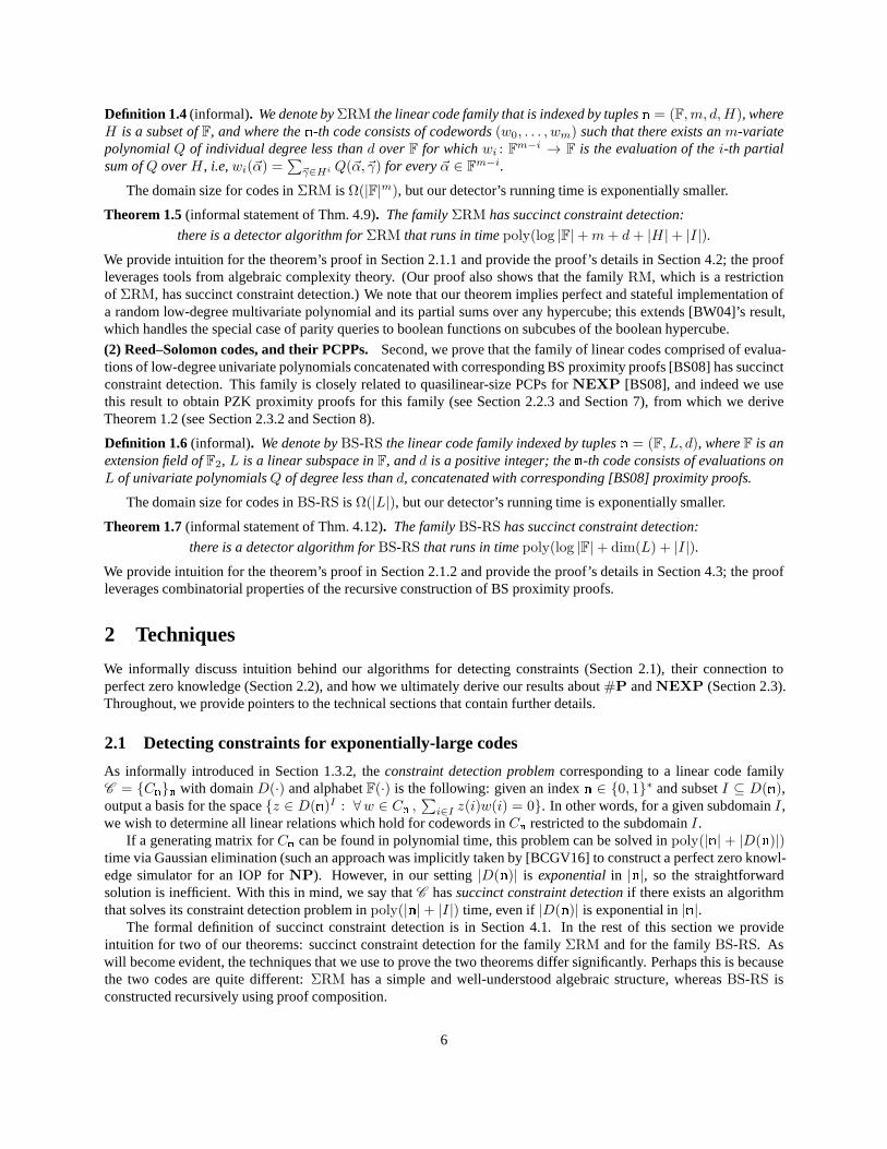
Definition 1.4 (informal). We denote byΣRM the linear code family that is indexed by tuplesn = (F,m, d,H), whereH is a subset ofF, and where then-th code consists of codewords(w0, . . . , wm) such that there exists anm-variatepolynomialQ of individual degree less thand overF for whichwi : F
m−i → F is the evaluation of thei-th partialsum ofQ overH , i.e,wi(~α) =
∑
~γ∈Hi Q(~α,~γ) for every~α ∈ Fm−i.
The domain size for codes inΣRM isΩ(|F|m), but our detector’s running time is exponentially smaller.
Theorem 1.5(informal statement of Thm. 4.9). The familyΣRM has succinct constraint detection:
there is a detector algorithm forΣRM that runs in timepoly(log |F|+m+ d+ |H |+ |I|).We provide intuition for the theorem’s proof in Section 2.1.1 and provide the proof’s details in Section 4.2; the proofleverages tools from algebraic complexity theory. (Our proof also shows that the familyRM, which is a restrictionof ΣRM, has succinct constraint detection.) We note that our theorem implies perfect and stateful implementation ofa random low-degree multivariate polynomial and its partial sums over any hypercube; this extends [BW04]’s result,which handles the special case of parity queries to boolean functions on subcubes of the boolean hypercube.
(2) Reed–Solomon codes, and their PCPPs.Second, we prove that the family of linear codes comprised ofevalua-tions of low-degree univariate polynomials concatenated with corresponding BS proximity proofs [BS08] has succinctconstraint detection. This family is closely related to quasilinear-size PCPs forNEXP [BS08], and indeed we usethis result to obtain PZK proximity proofs for this family (see Section 2.2.3 and Section 7), from which we deriveTheorem 1.2 (see Section 2.3.2 and Section 8).
Definition 1.6 (informal). We denote byBS-RS the linear code family indexed by tuplesn = (F, L, d), whereF is anextension field ofF2, L is a linear subspace inF, andd is a positive integer; then-th code consists of evaluations onL of univariate polynomialsQ of degree less thand, concatenated with corresponding [BS08] proximity proofs.
The domain size for codes inBS-RS isΩ(|L|), but our detector’s running time is exponentially smaller.
Theorem 1.7(informal statement of Thm. 4.12). The familyBS-RS has succinct constraint detection:
there is a detector algorithm forBS-RS that runs in timepoly(log |F|+ dim(L) + |I|).We provide intuition for the theorem’s proof in Section 2.1.2 and provide the proof’s details in Section 4.3; the proofleverages combinatorial properties of the recursive construction of BS proximity proofs.
2 Techniques
We informally discuss intuition behind our algorithms for detecting constraints (Section 2.1), their connection toperfect zero knowledge (Section 2.2), and how we ultimatelyderive our results about#P andNEXP (Section 2.3).Throughout, we provide pointers to the technical sections that contain further details.
2.1 Detecting constraints for exponentially-large codes
As informally introduced in Section 1.3.2, theconstraint detection problemcorresponding to a linear code familyC = C
n
n
with domainD(·) and alphabetF(·) is the following: given an indexn ∈ 0, 1∗ and subsetI ⊆ D(n),output a basis for the spacez ∈ D(n)I : ∀w ∈ C
n
,∑
i∈I z(i)w(i) = 0. In other words, for a given subdomainI,we wish to determine all linear relations which hold for codewords inC
n
restricted to the subdomainI.If a generating matrix forC
n
can be found in polynomial time, this problem can be solved inpoly(|n| + |D(n)|)time via Gaussian elimination (such an approach was implicitly taken by [BCGV16] to construct a perfect zero knowl-edge simulator for an IOP forNP). However, in our setting|D(n)| is exponentialin |n|, so the straightforwardsolution is inefficient. With this in mind, we say thatC hassuccinct constraint detectionif there exists an algorithmthat solves its constraint detection problem inpoly(|n|+ |I|) time, even if|D(n)| is exponential in|n|.
The formal definition of succinct constraint detection is inSection 4.1. In the rest of this section we provideintuition for two of our theorems: succinct constraint detection for the familyΣRM and for the familyBS-RS. Aswill become evident, the techniques that we use to prove the two theorems differ significantly. Perhaps this is becausethe two codes are quite different:ΣRM has a simple and well-understood algebraic structure, whereasBS-RS isconstructed recursively using proof composition.
6
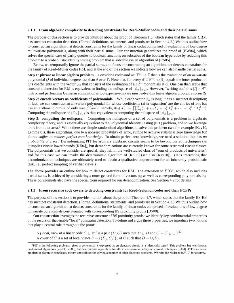
2.1.1 From algebraic complexity to detecting constraints for Reed–Muller codes and their partial sums
The purpose of this section is to provide intuition about theproof of Theorem 1.5, which states that the familyΣRMhas succinct constraint detection. (Formal definitions, statements, and proofs are in Section 4.2.) We thus outline howto construct an algorithm that detects constraints for the family of linear codes comprised of evaluations of low-degreemultivariate polynomials, along with their partial sums. Our construction generalizes the proof of [BW04], whichsolves the special case of parity queries to boolean functions on subcubes of the boolean hypercube by reducing thisproblem to a probabilistic identity testing problem that issolvable via an algorithm of [RS05].
Below, we temporarily ignore the partial sums, and focus on constructing an algorithm that detects constraints forthe family of Reed–Muller codesRM, and at the end of the section we indicate how we can also handle partial sums.
Step 1: phrase as linear algebra problem. Consider a codewordw : Fm → F that is the evaluation of anm-variatepolynomialQ of individual degree less thand overF. Note that, for every~α ∈ F
m, w(~α) equals the inner product ofQ’s coefficients with the vectorφ~α that consists of the evaluation of alldm monomials at~α. One can then argue thatconstraint detection forRM is equivalent to finding the nullspace ofφ~α~α∈I . However, “writing out” this|I| × dmmatrix and performing Gaussian elimination is too expensive, so we must solve this linear algebra problemsuccinctly.
Step 2: encode vectors as coefficients of polynomials.While each vectorφ~α is long, it has a succinct description;in fact, we can construct anm-variate polynomialΦ~α whose coefficients (after expansion) are the entries ofφ~α, buthas an arithmetic circuit of only sizeO(md): namely,Φ~α( ~X) :=
∏mi=1(1 + αiXi + α2
iX2i + · · · + αd−1
i Xd−1i ).
Computing the nullspace ofΦ~α~α∈I is thus equivalent to computing the nullspace ofφ~α~α∈I .
Step 3: computing the nullspace. Computing the nullspace of a set of polynomials is a problem in algebraiccomplexity theory, and is essentially equivalent to the Polynomial Identity Testing (PIT) problem, and so we leveragetools from that area.2 While there are simple randomized algorithms to solve this problem (see for example [Kay10,Lemma 8]), these algorithms, due to a nonzero probability oferror, suffice to achieve statistical zero knowledgebutdo not suffice to achieve perfect zero knowledge. To obtain perfect zero knowledge, we need a solution that has noprobability of error. Derandomizing PIT for arbitrary algebraic circuits seemsto be beyond current techniques (asit implies circuit lower bounds [KI04]), but derandomizations are currently known for some restricted circuit classes.The polynomials that we consider are special: they fall in the well-studied class of “sum of products of univariates”,and for this case we can invoke the deterministic algorithm of [RS05] (see also [Kay10]). (It is interesting thatderandomization techniques are ultimately used to obtain aqualitative improvement for an inherently probabilistictask, i.e., perfect sampling of verifier views.)
The above provides an outline for how to detect constraints for RM. The extension toΣRM, which also includespartial sums, is achieved by considering a more general formof vectorsφ~α as well as corresponding polynomialsΦ~α.These polynomials also have the special form required for our derandomization. See Section 4.2 for details.
2.1.2 From recursive code covers to detecting constraints for Reed–Solomon codes and their PCPPs
The purpose of this section is to provide intuition about theproof of Theorem 1.7, which states that the familyBS-RShas succinct constraint detection. (Formal definitions, statements, and proofs are in Section 4.3.) We thus outline howto construct an algorithm that detects constraints for the family of linear codes comprised of evaluations of low-degreeunivariate polynomials concatenated with corresponding BS proximity proofs [BS08].
Our construction leverages the recursive structure of BS proximity proofs: we identify key combinatorial propertiesof the recursion that enable “local” constraint detection.To define and argue these properties, we introduce two notionsthat play a central role throughout the proof:
A (local) viewof a linear codeC ⊆ FD is a pair(D, C) such thatD ⊆ D andC = C|D ⊆ F
D.A coverof C is a set of local viewsS = (Dj , Cj)j of C such thatD = ∪jDj .
2PIT is the following problem: given a polynomialf expressed as an algebraic circuit, isf identically zero? This problem has well-knownrandomized algorithms [Zip79, Sch80], but deterministic algorithms for all circuits seem to be beyond current techniques [KI04]. PIT is a centralproblem in algebraic complexity theory, and suffices for solving a number of other algebraic problems. We refer the reader to [SY10] for a survey.
7

Combinatorial properties of the recursive step. Given a finite fieldF, domainD ⊆ F, and degreed, let C :=RS[F, D, d] be the Reed–Solomon code consisting of evaluations onD of univariate polynomials of degree less thand overF; for concreteness, say that the domain size is|D| = 2n and the degree isd = |D|/2 = 2n−1.
The first level of [BS08]’s recursion appends to each codeword f ∈ C an auxiliary functionπ1(f) : D′ → F withdomainD′ disjoint fromD. Moreover, the mapping fromf toπ1(f) is linear overF, so the setC1 := f‖π1(f)f∈C ,wheref‖π1(f) : D ∪D′ → F is the function that agrees withf onD and withπ1(f) onD′, is a linear code overF.The codeC1 is the “first-level” code of a BS proximity proof forf .
The codeC1 has a naturally defined coverS1 = (Dj , Cj)j such that eachCj is a Reed–Solomon codeRS[F, Dj , dj ] with 2dj ≤ |Dj | = O(
√d), that is, with rate1/2 and block lengthO(
√d). We prove several com-
binatorial properties of this cover:
• S1 is 1-intersecting.For all distinctj, j′ in J , |Dj ∩ Dj′ | ≤ 1 (namely, the subdomains are almost disjoint).
• S1 isO(√d)-local. Every partial assignment toO(
√d) domainsDj in the cover that islocally consistentwith the
cover can be extended to aglobally consistentassignment, i.e., to a codeword ofC1. That is, there existsκ = O(√d)
such that every partial assignmenth : ∪κℓ=1 Djℓ → F with h|Djℓ∈ Cjℓ (for eachℓ) equals the restriction to the
subdomain∪κℓ=1Djℓ of some codewordf‖π1(f) in C1.
• S1 isO(√d)-independent. The ability to extend locally-consistent assignments to “globally-consistent” codewords
of C1 holds in a stronger sense: even when the aforementioned partial assignmenth is extendedarbitrarily to κadditional point-value pairs, this new partial assignmentstill equals the restriction of some codewordf‖π1(f) inC1.
The locality property alone already suffices to imply that given a subdomainI ⊆ D ∪ D′ of size|I| <√d, we can
solve the constraint detection problem onI by considering only those constraints that appear in views that intersectI(see Lemma 4.22). ButC has exponential block length so a “quadratic speedup” does not yet imply succinct constraintdetection. To obtain it, we also leverage the intersection and independence properties to reduce “locality” as follows.
Further recursive steps. So far we have only considered the first recursive step of a BS proximity proof; weshow how to obtain covers with smaller locality (and therebydetect constraints with more efficiency) by consideringadditional recursive steps. Each codeCj in the coverS1 ofC1 is a Reed–Solomon codeRS[F, Dj , dj ] with |Dj |, dj =O(√d), and the next recursive step appends to each codeword inCj a corresponding auxiliary function, yielding a
new codeC2. In turn,C2 has a coverS2, and another recursive step yields a new codeC3, which has its own coverS3,and so on. The crucial technical observation (Lemma 4.20) isthat the intersection and independence properties, whichhold recursively, enable us to deduce thatCi is 1-intersecting,O( 2i
√d)-local, andO( 2i
√d)-independent; in particular,
for r = log log d+O(1), Sr is 1-intersecting,O(1)-local,O(1)-independent.Then, recalling that detecting constraints for local codesrequires only the views in the cover that intersectI
(Lemma 4.22), our constraint detector works by choosingi ∈ 1, . . . , r such that the coverSi is poly(|I|)-local,finding in this cover apoly(|I|)-size set ofpoly(|I|)-size views that intersectI, and computing inpoly(|I|) time abasis for the dual of each of these views — thereby proving Theorem 1.7.
Remark 2.1. For the sake of those familiar withBS-RS we remark that the domainD′ is the carefully chosen subsetof F×F designated by that construction, the codeC1 is the code that evaluates bivariate polynomials of degreeO(
√d)
onD ∪D′ (along the way mappingD ⊆ F to a subset ofF× F), the subdomainsDj are the axis-parallel “rows” and“columns” used in that recursive construction, and the codesCj are Reed–Solomon codes of block lengthO(
√d). The
O(√d)-locality and independence follow from basic properties ofbivariate Reed–Muller codes; see Example 4.14.
Remark 2.2. It is interesting to compare the above result withlinear lower bounds on query complexityfor testingproximity to random low density parity check (LDPC) codes [BHR05, BGK+10]. Those results are proved by ob-taining a basis for the dual code such that every small-support constraint is spanned by a small subset of that basis.The same can be observed to hold forBS-RS, even though this latter code is locally testable withpolylogarithmicquery complexity[BS08, Thm. 2.13]. The difference between the two cases is due to the fact that, for a random LDPCcode, an assignment that satisfies all but a single basis-constraint is (with high probability) far from the code, whereasthe recursive and1-intersecting structure ofBS-RS implies the existence of words that satisfy all but a single basisconstraint, yet are negligibly close to being a codeword.
8

2.2 From constraint detection to perfect zero knowledge viamasking
We provide intuition about the connection between constraint detection and perfect zero knowledge (Section 2.2.1),and how we leverage this connection to achieve two intermediate results: (i) a sumcheck protocol that is perfect zeroknowledge in the Interactive PCP model (Section 2.2.2); and(ii) proximity proofs for Reed–Solomon codes that areperfect zero knowledge in the Interactive Oracle Proof model (Section 2.2.3).
2.2.1 Local simulation of random codewords
Suppose that the prover and verifier both have oracle access to a codewordw ∈ C, for some linear codeC ⊆ FD with
exponential-size domainD, and that they need to engage in some protocol that involvesw. During the protocol, theprover may leak information aboutw that is hard to compute (e.g., requires exponentially-manyqueries tow), and sowould violate zero knowledge (as we see below, this is the case for protocols such as sumcheck).
Rather than directly invoking the protocol, the prover firstsends to the verifier a random codewordr ∈ C (as anoracle sincer has exponential size) and the verifier replies with a random field elementρ ∈ F; then the prover andverifier invoke the protocol on the new codewordw′ := ρw+ r ∈ C rather thanw. Intuitively, running the protocol onw′ now does not leak information aboutw, becausew′ is random inC (up to resolvable technicalities). Thisrandomself-reducibilitymakes sense for only some protocols, e.g., those where completeness is preserved for any choice ofρand soundness is broken for only a small fraction ofρ; but this will indeed be the case for the settings described below.
The aforementionedmaskingtechnique was used by [BCGV16] for codes with polynomial-size domains, but weuse it for codes with exponential-size domains, which requires exponentially more efficient simulation techniques.Indeed, to prove perfect zero knowledge, a simulator must beable to reproduce, exactly, the view obtained by anymalicious verifier that queries entries ofw′, a uniformly random codeword inC; however, it is too expensive forthe simulator to explicitly sample a random codeword and answer the verifier’s queries according to it. Instead, thesimulator must sample the “local view” that the verifier seeswhile queryingw′ at asmallnumber of locationsI ⊆ D.
But simulating local views of the formw′|I is reducible to detectingconstraints, i.e., codewords in the dual codeC⊥ whose support is contained inI. Indeed, if no word inC⊥ has support contained inI thenw′|I is uniformlyrandom; otherwise, each additional linearly independent constraint ofC⊥ with support contained inI further reducesthe entropy ofw′|I in a well-understood manner. (See Lemma 4.3 for a formal statement.) In sum, succinct constraintdetection enables us to “implement” [GGN10, BW04] random codewords ofC despiteC having exponential size.
We now discuss two concrete protocols for which the aforementioned random self-reducibility applies, and forwhich we also have constructed suitably-efficient constraint detectors.
2.2.2 Perfect zero knowledge sumchecks
The celebrated sumcheck protocol [LFKN92] isnotzero knowledge. In the sumcheck protocol, the prover and verifierhave oracle access to a low-degreem-variate polynomialF over a fieldF, and the prover wants to convince the verifierthat
∑
~α∈Hm F (~α) = 0 for a given subsetH of F. During the protocol, the prover communicates partial sumsof F ,which are#P-hard to compute and, as such, violate zero knowledge.
We now explain how to use random self-reducibility to make the sumcheck protocolperfect zero knowledge, at thecost of moving from the Interactive Proof model to the Interactive PCP model.
IPCP sumcheck. Consider the following tweak to the classical sumcheck protocol: rather than invoking sumcheckonF directly, the prover first sends to the verifier a random low-degree polynomialR that sums to zero onHm (as anoracle), the verifier replies with a random field elementρ, and then the two invoke sumcheck onQ := ρF +R instead.
Completeness is clear because if∑
~α∈Hm F (~α) = 0 and∑
~α∈Hm R(~α) = 0 then∑
~α∈Hm(ρF + R)(~α) = 0;soundness is also clear because if
∑
~α∈Hm F (~α) 6= 0 then∑
~α∈Hm(ρF + R)(~α) 6= 0 with high probability overρ,regardless of the choice ofR. (For simplicity, we ignore the fact that the verifier also needs to test thatR has lowdegree.) We are thus left to show perfect zero knowledge, which turns out to be a much less straightforward argument.
The simulator. Before we explain how to argue perfect zero knowledge, we first clarify what we mean by it: sincethe verifier has oracle access toF we cannot hope to ‘hide’ it; nevertheless, we can hope to argue that the verifier, byparticipating in the protocol, does not learn anything about F beyond what the verifier can directly learn by querying
9

F (and the fact thatF sums to zero onHm). What we shall achieve is the following: an algorithm that simulates theverifier’s view by making as many queries toF as thetotal number of verifier queries to eitherF orR.
On the surface, perfect zero knowledge seems easy to argue, becauseρF + R seems random among low-degreem-variate polynomials that sum to zero onHm. More precisely, consider the simulator that samples a random low-degree polynomialQ that sums to zero onHm and uses it instead ofρF + R and answers the verifier queries asfollows: (a) whenever the verifier queriesF (~α), respond by queryingF (~α) and returning the true value; (b) wheneverthe verifier queriesR(~α), respond by queryingF (~α) and returningQ(~α) − ρF (~α). Observe that the number ofqueries toF made by the simulator equals the number of (mutually) distinct queries toF andR made by the verifier,as desired.
However, the above reasoning, while compelling, is insufficient. First,ρF +R is not random because a maliciousverifier can chooseρ depending on queries toR. Second, even ifρF +R were random (e.g., the verifier does not queryR before choosingρ), the simulator must run in polynomial time, both producingcorrectly-distributed ‘partial sums’of ρF + R and answering queries toR, but samplingQ alone requires exponential time. In this high level discussionwe ignore the first problem (which nonetheless has to be tackled), and focus on the second.
At this point it should be clear from the discussion in Section 2.2.1 that the simulator does not have to sampleQexplicitly, but only has to perfectly simulate local views of it by leveraging the fact that it can keep state across queries.And doing so requires solving the succinct constraint detection problem for a suitable codeC. In this case, it sufficesto consider the codeC = ΣRM, and our Theorem 1.5 guarantees the required constraint detector.
The above discussion omits several details, so we refer the reader to Section 5 for further details.
2.2.3 Perfect zero knowledge proximity proofs for Reed–Solomon
Testing proximity of a codewordw to a given linear codeC can be aided by aproximity proof [DR04, BGH+06],which is an auxiliary oracleπ that facilitates testing (e.g.,C is not locally testable). For example, testing proximity tothe Reed–Solomon code, a crucial step towards achieving short PCPs, is aided via suitable proximity proofs [BS08].
From the perspective of zero knowledge, however, a proximity proof can be ‘dangerous’: a few locations ofπ canin principle leak a lot of information about the codewordw, and a malicious verifier could potentially learn a lot aboutw with only a few queries tow andπ. The notion of zero knowledge for proximity proofs requiresthat this cannothappen: it requires the existence of an algorithm that simulates the verifier’s view by making as many queries tow asthe total number of verifier queries to eitherw or π [IW14]; intuitively, this means that any bit of the proximity proofπ reveals no more information than one bit ofw.
We demonstrate again the use of random self-reducibility and show a general transformation that, under certainconditions, maps a PCP of proximity(P, V ) for a codeC to a corresponding2-round Interactive Oracle Proof ofProximity (IOPP) forC that isperfect zero knowledge.
IOP of proximity for C. Consider the following IOP of Proximity: the prover and verifier have oracle access to acodewordw, and the prover wants to convince the verifier thatw is close toC; the prover first sends to the verifier arandom codewordr in C, and the verifier replies with a random field elementρ; the prover then sends the proximityproofπ′ := P (w′) that attests thatw′ := ρw + r is close toC. Note that this is a2-round IOP of Proximity forC,because completeness follows from the fact thatC is linear, while soundness follows because ifw is far fromC, thenso isρw + r for everyr with high probability overρ. But is the perfect zero knowledge property satisfied?
The simulator. Without going into details, analogously to Section 2.2.2, asimulator must be able to sample localviews for random codewords from the codeL := w‖P (w) w∈C , so the simulator’s efficiency reduces to the effi-ciency of constraint detection forL. We indeed prove that ifL has succinct constraint detection then the simulatorworks out. See Section 7.1 for further details.
The case of Reed–Solomon.The above machinery allows us to derive a perfect zero knowledge IOP of Proximityfor Reed–Solomon codes, thanks to our Theorem 1.7, which states that the family of linear codes comprised of evalua-tions of low-degree univariate polynomials concatenated with corresponding BS proximity proofs [BS08] has succinctconstraint detection; see Section 7.2 for details. This is one of the building blocks of our construction of perfect zeroknowledge IOPs forNEXP, as described below in Section 2.3.2.
10

2.3 Achieving perfect zero knowledge beyondNP
We outline how to derive our results about perfect zero knowledge for#P andNEXP.
2.3.1 Perfect zero knowledge for counting problems
We provide intuition for the proof of Theorem 1.1, which states that the complexity class#P has Interactive PCPsthat are perfect zero knowledge.
We first recall the classical (non zero knowledge) Interactive Proof for#P [LFKN92]. The languageL#3SAT,which consists of pairs(φ,N) whereφ is a3-CNF boolean formula andN is the number of satisfying assignments ofφ, is#P-complete, and thus it suffices to construct an IP for it. The IP forL#3SAT works as follows: the prover andverifier botharithmetizeφ to obtain a low-degree multivariate polynomialpφ and invoke the (non zero knowledge)sumcheck protocol on the claim “
∑
~α∈0,1n pφ(~α) = N ”, where arithmetic is over a large-enough prime field.Returning to our goal, we obtain a perfect zero knowledge Interactive PCP by simply replacing the (non zero knowl-
edge) IP sumcheck mentioned above with our perfect zero knowledge IPCP sumcheck, described in Section 2.2.2. InSection 6 we provide further details, including proving that the zero knowledge guarantees of our sumcheck protocolsuffice for this case.
2.3.2 Perfect zero knowledge for nondeterministic time
We provide intuition for the proof of Theorem 1.2, which implies that the complexity classNEXP has Interac-tive Oracle Proofs that are perfect zero knowledge. Very informally, the proof consists of combining two buildingblocks: (i) [BCGV16]’s reduction fromNEXP to randomizablelinear algebraic constraint satisfaction problems,and (ii) our construction of perfect zero knowledge IOPs of Proximity for Reed–Solomon codes, described in Sec-tion 2.2.3. Besides extending [BCGV16]’s result fromNP toNEXP, our proof provides a conceptual simplificationover [BCGV16] by clarifying how the above two building blocks work together towards the final result. We nowdiscuss this.
Starting point: [BS08]. Many PCP constructions consist of two steps: (1) arithmetize the statement at hand (in ourcase, membership of an instance in someNEXP-complete language) by reducing it to a “PCP-friendly” problem thatlooks like alinear-algebraicconstraint satisfaction problem (LACSP); (2) design a tester that probabilistically checkswitnesses for this LACSP. In this paper, as in [BCGV16], we take [BS08]’s PCPs forNEXP as a starting point,where the first step reducesNEXP to a “univariate” LACSP whose witnesses are codewords in a Reed–Solomoncode of exponential degree that satisfy certain properties, and whose second step relies on suitableproximity proofs[DR04, BGH+06] for that code. Thus, overall, the PCP consists of two oracles, one being the LACSP witness andthe other being the corresponding BS proximity proof, and itis not hard to see that such a PCP isnot zero knowledge,because both the LACSP witness and its proximity proof reveal hard-to-compute information.
Step 1: sanitize the proximity proof. We first address the problem that the BS proximity proof “leaks”, by simplyreplacing it with our own perfect zero knowledge analogue. Namely, we replace it with our perfect zero knowledge2-round IOP of Proximity for Reed–Solomon codes, described in Section 2.2.3. This modification ensures that thereexists an algorithm that perfectly simulates the verifier’sview by making as many queries to the LACSP witness as thetotal number of verifier queries toeither the LACSP witness or other oracles used to facilitateproximity testing. At thispoint we have obtained a perfect zero knowledge2-round IOP of Proximity forNEXP (analogous to the notion of azero knowledge PCP of Proximity [IW14]); this part is where,previously, [BCGV16] were restricted toNP becausetheir simulator only handled Reed–Solomon codes withpolynomialdegree while our simulator is efficient even forsuch codes withexponentialdegree. But we are not done yet: to obtain our goal, we also need to address the problemthat the LACSP witness itself “leaks” when the verifier queries it, which we discuss next.
Step 2: sanitize the witness. Intuitively, we need to inject randomness in the reduction from NEXP to LACSPbecause the prover ultimately sends an LACSP witness to the verifier as an oracle, which the verifier can query. This isprecisely what [BCGV16]’s reduction fromNEXP to randomizableLACSPs enables, and we thus use their reductionto complete our proof. Informally, given an a-priori query boundb on the verifier’s queries, the reduction outputs awitnessw with the property that one can efficiently sampleanotherwitnessw′ whose entries areb-wise independent.We can then simply use the IOP of Proximity from the previous step on this randomized witness. Moreover, since the
11

efficiency of the verifier is polylogarithmic inb, we can setb to be super-polynomial (e.g., exponential) to preservezero knowledge against any polynomial number of verifier queries.
The above discussion is only a sketch and we refer the reader to Section 8 for further details. One aspect that wedid not discuss is that an LACSP witness actually consists oftwo sub-witnesses, where one is a “local” deterministicfunction of the other, which makes arguing zero knowledge somewhat more delicate.
2.4 Roadmap
After providing formal definitions in Section 3.1, the rest of the paper is organized as summarized by the table below.
§4.2 Theorem 1.5/4.9 detecting constraints forΣRM §4.3 Theorem 1.7/4.12 detecting constraints forBS-RS
y
y
§5 Theorem 5.3 PZK IPCP for sumcheck §7 Theorem 7.3 PZK IOP of Proximity for RS codes
y
y
§6 Theorem 1.1/6.2 PZK IPCP for#P §8 Theorem 1.2/8.1 PZK IOP forNEXP
12

3 Definitions
3.1 Basic notations
Functions, distributions, fields. We usef : D → R to denote a function with domainD and rangeR; given a subsetD of D, we usef |D to denote the restriction off to D. Given a distributionD, we writex ← D to denote thatxis sampled according toD. We denote byF a finite field and byFq the field of sizeq; we sayF is abinary field ifits characteristic is2. Arithmetic operations overFq costpolylog q but we shall consider these to have unit cost (andinspection shows that accounting for their actual polylogarithmic cost does not change any of the stated results).
Distances. A distance measure is a function∆: Σn × Σn → [0, 1] such that for allx, y, z ∈ Σn: (i) ∆(x, x) = 0,(ii) ∆(x, y) = ∆(y, x), and (iii)∆(x, y) ≤ ∆(x, z) + ∆(z, y). We extend∆ to distances to sets: givenx ∈ Σn andS ⊆ Σn, we define∆(x, S) := miny∈S ∆(x, y) (or 1 if S is empty). We say that a stringx is ǫ-close to another stringy if ∆(x, y) ≤ ǫ, andǫ-far fromy if ∆(x, y) > ǫ; similar terminology applies for a stringx and a setS. Unless notedotherwise, we use therelative Hamming distanceover alphabetΣ (typically implicit): ∆(x, y) := |i : xi 6= yi|/n.
Languages and relations. We denote byR a (binary ordered) relation consisting of pairs(x,w), wherex is theinstanceandw is thewitness. We denote byLan(R) the language corresponding toR, and byR|
x
the set of witnessesin R for x (if x 6∈ Lan(R) thenR|
x
:= ∅). As always, we assume that|w| is bounded by some computable functionof n := |x|; in fact, we are mainly interested in relations arising fromnondeterministic languages:R ∈ NTIME(T )if there exists aT (n)-time machineM such thatM(x,w) outputs1 if and only if (x,w) ∈ R. Throughout, we assumethatT (n) ≥ n. We say thatR has relative distanceδR : N→ [0, 1] if δR(n) is the minimum relative distance amongwitnesses inR|
x
for all x of sizen. Throughout, we assume thatδR is a constant.
Polynomials. We denote byF[X1, . . . , Xm] the ring of polynomials inm variables overF. Given a polynomialPin F[X1, . . . , Xm], degXi
(P ) is the degree ofP in the variableXi. We denote byF<d[X1, . . . , Xm] the subspaceconsisting ofP ∈ F[X1, . . . , Xm] with degXi
(P ) < d for everyi ∈ 1, . . . ,m.Random shifts. We later use a folklore claim about distance preservation for random shifts in linear spaces.
Claim 3.1. Letn be inN, F a finite field,S anF-linear space inFn, andx, y ∈ Fn. If x is ǫ-far fromS, thenαx+ y
is ǫ/2-far fromS, with probability1− |F|−1 over a randomα ∈ F. (Distances are relative Hamming distances.)
3.2 Single-prover proof systems
We use two types of proof systems that combine aspects of interactive proofs [Bab85, GMR89] and probabilisti-cally checkable proofs [BFLS91, AS98, ALM+98]: interactive PCPs(IPCPs) [KR08] andinteractive oracle proofs(IOPs) [BCS16, RRR16]. We first describe IPCPs (Section 3.2.1) and then IOPs (Section 3.2.2), which generalize theformer.
3.2.1 Interactive probabilistically checkable proofs
An IPCP [KR08] is a PCP followed by an IP. Namely, the proverP and verifierV interact as follows:P sends toV aprobabilistically checkable proofπ; afterwards,P andV π engage in an interactive proof. Thus,V may read a few bitsof π but must read subsequent messages fromP in full. An IPCP systemfor a relationR is thus a pair(P, V ), whereP, V are probabilistic interactive algorithms working as described, that satisfies naturally-defined notions of perfectcompleteness and soundness with a given errorε(·); see [KR08] for details.
We say that an IPCP hask rounds if this “PCP round” is followed by a(k − 1)-round interactive proof. (That is,we count the PCP round towards round complexity, unlike [KR08].) Beyond round complexity, we also measure howmany bits the prover sends and how many the verifier reads: theproof lengthl is the length ofπ in bits plus the numberof bits in all subsequent prover messages; thequery complexityq is the number of bits ofπ read by the verifier plusthe number of bits in all subsequent prover messages (since the verifier must read all of those bits).
In this work, we do not count the number of bits in the verifier messages, nor the number of random bits used bythe verifier; both are bounded from above by the verifier’s running time, which we do consider. Overall, we say thata relationR belongs to the complexity classIPCP[k, l, q, ε, tp, tv] if there is an IOP system forR in which: (1) the
13

number of rounds is at mostk(n); (2) the proof length is at mostl(n); (3) the query complexity is at mostq(n); (4) thesoundness error isε(n); (5) the prover algorithm runs in timetp(n); (6) the verifier algorithm runs in timetv(n).
3.2.2 Interactive oracle proofs
An IOP [BCS16, RRR16] is a “multi-round PCP”. That is, an IOP generalizes an interactive proof as follows: when-ever the prover sends to the verifier a message, the verifier does not have to read the message in full but may probabilis-tically query it. In more detail, ak-round IOP comprisesk rounds of interaction. In thei-th round of interaction: theverifier sends a messagemi to the prover; then the prover replies with a messageπi to the verifier, which the verifiercan query in this and later rounds (via oracle queries). After thek rounds of interaction, the verifier either accepts orrejects.
An IOP systemfor a relationR with soundness errorε is thus a pair(P, V ), whereP, V are probabilistic interactivealgorithms working as described, that satisfies the following properties. (See [BCS16] for more details.)
Completeness:For every instance-witness pair(x,w) in the relationR, Pr[〈P (x,w), V (x)〉 = 1] = 1.
Soundness:For every instancex not inR’s language and unbounded malicious proverP , Pr[〈P , V (x)〉 = 1] ≤ ε(n).
Beyond round complexity, we also measure how many bits the prover sends and how many the verifier reads: theproof lengthl is the total number of bits in all of the prover’s messages, and thequery complexityq is the total numberof bits read by the verifier across all of the prover’s messages. Considering all of these parameters, we say that arelationR belongs to the complexity classIOP[k, l, q, ε, tp, tv] if there is an IOP system forR in which: (1) thenumber of rounds is at mostk(n); (2) the proof length is at mostl(n); (3) the query complexity is at mostq(n); (4) thesoundness error isε(n); (5) the prover algorithm runs in timetp(n); (6) the verifier algorithm runs in timetv(n).
IOP vs. IPCP. An IPCP (see Section 3.2.1) is a special case of an IOP becausean IPCP verifier must read in full allof the prover’s messages except the first one (while an IOP verifier may query any part of any prover message). Theabove complexity measures are consistent with those definedfor IPCPs.
3.2.3 Restrictions and extensions
The definitions below are about IOPs, but IPCPs inherit all ofthese definitions because they are a special case of IOP.
Adaptivity of queries. An IOP system isnon-adaptiveif the verifier queries are non-adaptive, i.e., the queriedlocations depend only on the verifier’s inputs.
Public coins. An IOP system ispublic coin if each verifier messagemi is chosen uniformly and independently atrandom, and all of the verifier queries happen after receiving the last prover message.
Proximity. An IOP of proximityextends the definition of an IOP in the same way that a PCP of proximity extendsthat of a PCP [DR04, BGH+06]. An IOPP systemfor a relationR with soundness errorε and proximity parameterδis a pair(P, V ) that satisfies the following properties.
Completeness:For every instance-witness pair(x,w) in the relationR, Pr[〈P (x,w), V w(x)〉 = 1] = 1.
Soundness:For every instance-witness pair(x,w) with ∆(w,R|x
) ≥ δ(n) and unbounded malicious proverP ,Pr[〈P , V w(x)〉 = 1] ≤ ε(n).
Similarly to above, a relationR belongs to the complexity classIOPP[k, l, q, ε, δ, tp, tv] if there is an IOPP systemfor R with the corresponding parameters.
Promise relations. A promise relationis a relation-language pair(RYES,L NO) with Lan(RYES)∩LNO = ∅. An IOP
for a promise relation is the same as an IOP for the (standard)relationRYES, except that soundness need only holdfor x ∈ L NO. An IOPP for a promise relation is the same as an IOPP for the (standard) relationRYES, except thatsoundness need only hold forx ∈ Lan(RYES) ∪L NO.
14

3.2.4 Prior constructions
In this paper we give new IPCP and IOP constructions that achieve perfect zero knowledge for various settings. Belowwe summarize known constructions in these two models.
IPCPs. Prior work obtains IPCPs with proof length that depends on the witness size rather than computation size[KR08, GKR08], and IPCPs with statistical zero knowledge [GIMS10] (see Section 3.3 for more details).
IOPs. Prior work obtains IOPs with perfect zero knowledge forNP [BCGV16], IOPs with small proof length andquery complexity [BCG+16], and an amortization theorem for “unambiguous” IOPs [RRR16]. Also, [BCS16] showhow to compile public-coin IOPs into non-interactive proofs in the random oracle model.
3.3 Zero knowledge
We define the notion of zero knowledge for IOPs and IPCPs achieved by our constructions:perfect zero knowledge viastraightline simulators. This notion is quite strong not only because it unconditionally guarantees perfect simulationof the verifier’s view but also because straightline simulation implies desirable properties such as composability. Wenow provide some context and then give formal definitions.
At a high level, zero knowledge requires that the verifier’s view can be efficiently simulated without the prover.Converting the informal statement into a mathematical one involves many choices, including choosing which verifierclass to consider (e.g., the honest verifier? all polynomial-time verifiers?), the quality of the simulation (e.g., is itidentically distributed to the view? statistically close to it? computationally close to it?), the simulator’s dependenceon the verifier (e.g., is it non-uniform? or is the simulator universal?), and others. The definitions below consider twovariants: perfect simulation via universal simulators against either unbounded-query or bounded-query verifiers.
Moreover, in the case of universal simulators, one distinguishes between a non-blackbox use of the verifier, whichmeans that the simulator takes the verifier’s code as input, and a blackbox use of it, which means that the simulatoronly accesses the verifier via a restricted interface; we consider this latter case. Different models of proof systems callfor different interfaces, which grant carefully-chosen “extra powers” to the simulator (in comparison to the prover) soto ensure that efficiency of the simulation does not imply theability to efficiently decide the language. For example: inZK IPs, the simulator may rewind the verifier; in ZK PCPs, the simulator may adaptively answer oracle queries. In ZKIPCPs and ZK IOPs (our setting), the natural definition wouldallow a blackbox simulator to rewind the verifierandalsoto adaptively answer oracle queries. The definitions below,however, consider only simulators that are straightline[FS89, DS98], that is they do not rewind the verifier, becauseour constructions achieve this stronger notion.
Recall that protocols that are perfectly secure with a straightline simulator (in the standalone model) remain secureunder concurrent general composition [KLR10]. In particular, the above notion of zero knowledge is preserved undersuch composition and, for example, one can use parallel repetition to reduce soundness error without impacting zeroknowledge. Indeed, straightline simulation facilitates many applications, e.g., verifiable secret sharing in [IW14], andunconditional general universally-composable secure computation in [GIMS10].
We are now ready to define the notion of perfect zero knowledgevia straightline simulators. We first discuss thenotion for IOPs, then for IOPs of proximity, and finally for IPCPs.
3.3.1 ZK for IOPs
Below is the definition of perfect zero knowledge (via straightline simulators) for IOPs.
Definition 3.2. Let A,B be algorithms andx, y strings. We denote byView 〈B(y), A(x)〉 the view of A(x) inan interactive oracle protocol withB(y), i.e., the random variable(x, r, a1, . . . , an) wherex is A’s input, r is A’srandomness, anda1, . . . , an are the answers toA’s queries intoB’s messages.
Straightline simulators in the context of IPs were used in [FS89], and later defined in [DS98]. The definition belowconsiders this notion in the context of IOPs, where the simulator also has to answer oracle queries by the verifier. Notethat since we consider the notion of perfect zero knowledge,the definition of straightline simulation needs to allow theefficient simulator to work even with inefficient verifiers [GIMS10].
15

Definition 3.3. We say that an algorithmB hasstraightline accessto another algorithmA if B interacts withA,without rewinding, by exchanging messages withA and also answering any oracle queries along the way. We denotebyBA the concatenation ofA’s random tape andB’s output. (SinceA’s random tape could be super-polynomiallylarge,B cannot sample it forA and then output it; instead, we restrictB to not see it, and we prepend it toB’s output.)
Definition 3.4. An IOP system(P, V ) for a relationR is perfect zero knowledge (via straightline simulators) against unbounded queries(resp., against query boundb) if there exists a simulator algorithmS such that for every algorithm (resp.,b-query al-gorithm) V and instance-witness pair(x,w) ∈ R, SV (x) andView 〈P (x,w), V (x)〉 are identically distributed.Moreover,S must run in timepoly(|x|+ qV (|x|)), whereqV (·) is V ’s query complexity.
We say that a relationR belongs to the complexity classPZK-IOP[k, l, q, ε, tp, tv, b] if there is an IOP systemfor R, with the corresponding parameters, that is perfect zero knowledge with query boundb; also, it belongs to thecomplexity classPZK-IOP[k, l, q, ε, tp, tv, ∗] if the same is true with unbounded queries.
3.3.2 ZK for IOPs of proximity
Below is the definition of perfect zero knowledge (via straightline simulators) for IOPs of proximity. It is a straight-forward extension of the corresponding notion for PCPs of proximity, introduced in [IW14].
Definition 3.5. An IOPP system(P, V ) for a relation R is perfect zero knowledge (via straightline simulators)against unbounded queries(resp., against query boundb) if there exists a simulator algorithmS such that for everyalgorithm (resp.,b-query algorithm)V and instance-witness pair(x,w) ∈ R, the following two random variablesare identically distributed:
(
SV ,w(x) , qS
)
and(
View 〈P (x,w), V w(x)〉 , qV)
,
whereqS is the number of queries tow made byS, andqV is the number of queries tow or to prover messages madeby V . Moreover,S must run in timepoly(|x|+ qV (|x|)), whereqV (·) is V ’s query complexity.
We say that a relationR belongs to the complexity classPZK-IOPP[k, l, q, ε, δ, tp, tv, b] if there is an IOPPsystem forR, with the corresponding parameters, that is perfect zero knowledge with query boundb; also, it belongsto the complexity classPZK-IOPP[k, l, q, ε, δ, tp, tv, ∗] if the same is true with unbounded queries.
Remark 3.6. Analogously to [IW14], our definition of zero knowledge for IOPs of proximity requires that the numberof queries tow byS equals the total number of queries (tow or prover messages) byV . Stronger notions are possible:“the number of queries tow by S equals the number of queries tow by V ”; or, even more, “S andV read the samelocations ofw”. The definition above is sufficient for the applications of IOPs of proximity that we consider.
3.3.3 ZK for IPCPs
The definition of perfect zero knowledge (via straightline simulators) for IPCPs follows directly from Definition 3.4 inSection 3.3.1 because IPCPs are a special case of IOPs. Dittofor IPCPs of proximity, whose perfect zero knowledgedefinition follows directly from Definition 3.5 in Section 3.3.2. (For comparison, [GIMS10] define statistical zeroknowledge IPCPs, also with straightline simulators.)
3.4 Codes
An error correcting codeC is a set of functionsw : D → Σ, whereD,Σ are finite sets known as the domain andalphabet; we writeC ⊆ ΣD. The message length ofC is k := log|Σ| |C|, its block length isℓ := |D|, its rate isρ := k/ℓ, its (minimum) distance isd := min∆(w, z) : w, z ∈ C , w 6= z when∆ is the (absolute) Hammingdistance, and its (minimum) relative distance isτ := d/ℓ. At times we writek(C), ℓ(C), ρ(C), d(C), τ(C) to makethe code under consideration explicit. All the codes we consider are linear codes, discussed next.
16

Linearity. A codeC is linear if Σ is a finite field andC is aΣ-linear space inΣD. The dual code ofC is the setC⊥ of functionsz : D → Σ such that, for allw : D → Σ, 〈z, w〉 :=∑i∈D z(i)w(i) = 0. We denote bydim(C) thedimension ofC; it holds thatdim(C) + dim(C⊥) = ℓ anddim(C) = k (dimension equals message length).
Code families. A code familyC = Cn
n∈0,1∗ has domainD(·) and alphabetF(·) if each codeC
n
has domainD(n) and alphabetF(n). Similarly,C has message lengthk(·), block lengthℓ(·), rateρ(·), distanced(·), and relativedistanceτ(·) if each codeC
n
has message lengthk(n), block lengthℓ(n), rateρ(n), distanced(n), and relativedistanceτ(n). We also defineρ(C ) := inf
n∈N ρ(n) andτ(C ) := infn∈N τ(n).
Reed–Solomon codes.The Reed–Solomon (RS) code is the code consisting of evaluations ofunivariatelow-degreepolynomials: given a fieldF, subsetS of F, and positive integerd with d ≤ |S|, we denote byRS[F, S, d] the linearcode consisting of evaluationsw : S → F overS of polynomials inF<d[X ]. The code’s message length isk = d,block length isℓ = |S|, rate isρ = d
|S| , and relative distance isτ = 1− d−1|S| .
Reed–Muller codes. The Reed–Muller (RM) code is the code consisting of evaluations ofmultivariatelow-degreepolynomials: given a fieldF, subsetS of F, and positive integersm, d with d ≤ |S|, we denote byRM[F, S,m, d]the linear code consisting of evaluationsw : Sm → F overSm of polynomials inF<d[X1, . . . , Xm] (i.e., we boundindividual degrees rather than their sum). The code’s message length isk = dm, block length isℓ = |S|m, rate isρ = ( d
|S|)m, and relative distance isτ = (1 − d−1
|S| )m.
17
4 Succinct constraint detection
We introduce the notion ofsuccinct constraint detectionfor linear codes. This notion plays a crucial role in construct-ing perfect zero knowledge simulators for super-polynomial complexity classes (such as#P andNEXP), but webelieve that this naturally-defined notion is also of independent interest. Given a linear codeC ⊆ F
D we refer to itsdual codeC⊥ ⊆ F
D as theconstraint spaceof C. Theconstraint detection problemcorresponding to a family oflinear codesC = C
n
n
with domainD(·) and alphabetF(·) is the following:
Given an indexn and subsetI ⊆ D(n), output a basis forz ∈ D(n)I : ∀w ∈ Cn
,∑
i∈I z(i)w(i) = 0.3
If |D(n)| is polynomial in|n| and a generating matrix forCn
can be found in polynomial time, this problem canbe solved inpoly(|n| + |I|) time via Gaussian elimination; such an approach was implicitly taken by [BCGV16] toconstruct a perfect zero knowledge simulator for an IOP forNP. However, in our setting,|D(n)| is exponentialin |n|and|I|, and the aforementioned generic solution requires exponential time. With this in mind, we sayC hassuccinctconstraint detectionif there exists an algorithm that solves the constraint detection problem inpoly(|n| + |I|) timewhen|D(n)| is exponentialin |n|. After defining succinct constraint detection in Section 4.1, we proceed as follows.
• In Section 4.2, we construct a succinct constraint detectorfor the family of linear codes comprised of evaluations ofpartial sums of low-degree polynomials. The construction of the detector exploits derandomization techniques fromalgebraic complexity theory. Later on (in Section 5), we leverage this result to construct a perfect zero knowledgesimulator for an IPCP for#P.
• In Section 4.3, we construct a succinct constraint detectorfor the family of evaluations of univariate polynomialsconcatenated with corresponding BS proximity proofs [BS08]. The construction of the detector exploits the re-cursive structure of these proximity proofs. Later on (in Section 8), we leverage this result to construct a perfectzero knowledge simulator for an IOP forNEXP; this simulator can be interpreted as an analogue of [BCGV16]’ssimulator that runsexponentially fasterand thus enables us to “scale up” fromNP to NEXP.
Throughout this section we assume familiarity with terminology and notation about codes, introduced in Section 3.4.We assume for simplicity that|n|, the number of bits used to representn, is at leastlogD(n) + logF(n); if this doesnot hold, then one can replace|n| with |n|+ logD(n) + logF(n) throughout the section.
Remark 4.1 (sparse representation). In this section we make statements about vectorsv in FD where the cardinality
of the domainD may be super-polynomial. When such statements are computational in nature, we assume thatv is notrepresented as a list of|D| field elements (which requiresΩ(|D| log |F|) bits) but, instead, assume thatv is representedas a list of the elements insupp(v) (and each element comes with its index inD); this sparserepresentation onlyrequiresΩ(|supp(v)| · (log |D|+ log |F|)) bits.
4.1 Definition of succinct constraint detection
Formally define the notion of aconstraint detector, and the notion ofsuccinct constraint detection.
Definition 4.2. Let C = Cn
n
be a linear code family with domainD(·) and alphabetF(·). A constraint detectorfor C is an algorithm that, on input an indexn and subsetI ⊆ D(n), outputs a basis for the space
z ∈ D(n)I : ∀w ∈ Cn
,∑
i∈I
z(i)w(i)
.
We say thatC has aT (·, ·)-time constraint detectionif there exists a detector forC running in timeT (n, ℓ); we alsosay thatC hassuccinct constraint detectionif it haspoly(|n|+ ℓ)-time constraint detection.
3In fact, the following weaker definition suffices for the applications in our paper:given an indexn and subsetI ⊆ D(n), outputz ∈ F(n)I
such that∑
i∈I z(i)w(i) = 0 for all w ∈ Cn
, or ‘independent’ if no suchz exists. We achieve the stronger definition, which is also easier to workwith.
18

A constraint detector induces a corresponding probabilistic algorithm for ‘simulating’ answers to queries to arandom codeword; this is captured by the following lemma, the proof of which is in Appendix B. We shall use suchprobabilistic algorithms in the construction of perfect zero knowledge simulators (see Section 5 and Section 8).
Lemma 4.3. Let C = Cn
n
be a linear code family with domainD(·) and alphabetF(·) that hasT (·, ·)-timeconstraint detection. Then there exists a probabilistic algorithmA such that, for every indexn, set of pairsS =(α1, β1), . . . , (αℓ, βℓ) ⊆ D(n)× F(n), and pair(α, β) ∈ D(n) × F(n),
Pr[
A(n, S, α) = β]
= Prw←C
n
w(α) = β
∣
∣
∣
∣
∣
∣
∣
w(α1) = β1...
w(αℓ) = βℓ
.
MoreoverA runs in timeT (n, ℓ) + poly(log |F(n)| + ℓ).
For the purposes ofconstructinga constraint detector, the sufficient condition given in Lemma 4.6 below is some-times easier to work with. To state it we need to introduce twoways of restricting a code, and explain how theserestrictions interact with taking duals; the interplay between these is delicate (see Remark 4.7).
Definition 4.4. Given a linear codeC ⊆ FD and a subsetI ⊆ D, we denote by (i)C⊆I the set consisting of the
codewordsw ∈ C for whichsupp(w) ⊆ I, and (ii)C|I the restriction toI of codewordsw ∈ C.
Note thatC⊆I andC|I aredifferent notions. Consider for example the1-dimensional linear codeC = 00, 11in F
1,22 and the subsetI = 1: it holds thatC⊆I = 00 andC|I = 0, 1. In particular, codewords inC⊆I
are defined overD, while codewords inC|I are defined overI. Nevertheless, throughout this section, we sometimescompare vectors defined over different domains, with the implicit understanding that the comparison is conducted overthe union of the relevant domains, by filling in zeros in the vectors’ undefined coordinates. For example, we may writeC⊆I ⊆ C|I to mean that00 ⊆ 00, 10 (the set obtained from0, 1 after filling in the relevant zeros).
Claim 4.5. LetC be a linear code with domainD and alphabetF. For everyI ⊆ D,
(C|I)⊥ = (C⊥)⊆I ,
that is,
z ∈ D(n)I : ∀w ∈ Cn
,∑
i∈I
z(i)w(i)
=
z ∈ C⊥n
: supp(z) ⊆ I
.
Proof. For the containment(C⊥)⊆I ⊆ (C|I)⊥: if z ∈ C⊥ andsupp(z) ⊆ I thenz lies in the dual ofC|I becauseit suffices to consider the subdomainI for determining duality. For the reverse containment(C⊥)⊆I ⊇ (C|I)⊥: ifz ∈ (C|I)⊥ thensupp(z) ⊆ I (by definition) so that〈z, w〉 = 〈z, w|I〉 for everyw ∈ C, and the latter inner productequals0 becausez is in the dual ofC|I ; in sumz is dual to (all codewords in)C and its support is contained inI, soz belongs to(C⊥)⊆I , as claimed.
Observe that Claim 4.5 tells us the constraint detection is equivalent to determining a basis of(Cn
|I)⊥ = (C⊥n
)⊆I .The following lemma asserts that if, given a subsetI ⊆ D, we can find a set of constraintsW in C⊥ that spans(C⊥)⊆I then we can solve the constraint detection problem forC; we defer the proof of the lemma to Appendix C.
Lemma 4.6. LetC = Cn
n
be a linear code family with domainD(·) and alphabetF(·). If there exists an algorithmthat, on input an indexn and subsetI ⊆ D(n), outputs inpoly(|n| + |I|) time a subsetW ⊆ F(n)D(n) (in sparserepresentation) with(C⊥
n
)⊆I ⊆ span(W ) ⊆ C⊥n
, thenC has succinct constraint detection.
Remark 4.7. The following operations donot commute: (i) expanding the domain via zero padding (for the purposeof comparing vectors over different domains), and (ii) taking the dual of the code. Consider for example the codeC =
0 ⊆ F12 : its dual code isC⊥ = 0, 1 and, when expanded toF1,22 , the dual code is expanded to(0, 0), (1, 0);
yet, whenC is expanded toF1,22 it produces the code(0, 0) and its dual code is(0, 0), (1, 0), (0, 1), (1, 1). Toresolve ambiguities (when asserting an equality as in Claim4.5), we adopt the convention that expansion is donealways last(namely, as late as possible without having to compare vectors over different domains).
19

4.2 Partial sums of low-degree polynomials
We show that evaluations of partial sums of low-degree polynomials have succinct constraint detection (see Defini-tion 4.2). In the following,F is a finite field,m, d are positive integers, andH is a subset ofF; also,F<d[X1, . . . , Xm]denotes the subspace ofF[X1, . . . , Xm] consisting of those polynomials with individual degrees less thand. More-over, givenQ ∈ F
<d[X1, . . . , Xm] and ~α ∈ F≤m (vectors overF of length at mostm), we defineQ(~α) :=
∑
~γ∈Hm−|~α| Q(~α,~γ), i.e., the answer to a query that specifies only a suffix of the variables is the sum of the val-ues obtained by letting the remaining variables range overH . We begin by defining the code that we study, whichextends the Reed–Muller code (see Section 3.4) with partialsums.
Definition 4.8. We denote byΣRM[F,m, d,H ] the linear code that comprises evaluations of partial sums of polyno-mials inF<d[X1, . . . , Xm]; more precisely,ΣRM[F,m, d,H ] := wQQ∈F<d[X1,...,Xm] wherewQ : F≤m → F is thefunction defined bywQ(~α) :=
∑
~γ∈Hm−|~α| Q(~α,~γ) for each~α ∈ F≤m.4 We denote byΣRM the linear code family
indexed by tuplesn = (F,m, d,H) and where then-th code equalsΣRM[F,m, d,H ]. (We represent indicesn so toensure that|n| = Θ(log |F|+m+ d+ |H |).)
We prove that the linear code familyΣRM has succinct constraint detection:
Theorem 4.9(formal statement of 1.5). ΣRM haspoly(log |F|+m+ d+ |H |+ ℓ)-time constraint detection.
Combined with Lemma 4.3, the theorem above implies that there exists a probabilistic polynomial-time algorithmfor answering queries to a codeword sampled at random fromΣRM, as captured by the following corollary.
Corollary 4.10. There exists a probabilistic algorithmA such that, for every finite fieldF, positive integersm, d,subsetH of F, subsetS = (α1, β1), . . . , (αℓ, βℓ) ⊆ F
≤m × F, and(α, β) ∈ F≤m × F,
Pr[
A(F,m, d,H, S, α) = β]
= PrR←F<d[X1,...,Xm]
R(α) = β
∣
∣
∣
∣
∣
∣
∣
R(α1) = β1...
R(αℓ) = βℓ
.
MoreoverA runs in timepoly(log |F|+m+ d+ |H |+ ℓ).
We sketch the proof of Theorem 4.9, for the simpler case wherethe code isRM[F,m, d,H ] (i.e., without partialsums). We can view a polynomialQ ∈ F
<d[X1, . . . , Xm] as a vector over the monomial basis, with an entry for eachpossible monomialX i1
1 . . . X imm (with 0 ≤ i1, . . . , im < d) containing the corresponding coefficient. The evaluation
of Q at a point~α ∈ Fm then equals the inner product of this vector with the vectorφ~α, in the same basis, whose
entry forX i11 . . . X im
m is equal toαi11 . . . α
imm . Given~α1, . . . , ~αℓ, we could use Gaussian elimination onφ~α1
, . . . , φ~αℓ
to check for linear dependencies, which would be equivalentto constraint detection forRM[F,m, d,H ].However, we cannot afford to explicitly write downφ~α, because it hasdm entries. Nevertheless, we can still
implicitly check for linear dependencies, and we do so by reducing the problem, by building on and extending ideas of[BW04], to computing the nullspace of a certain set of polynomials, which can be solved via an algorithm of [RS05](see also [Kay10]). The idea is to encode the entries of thesevectors via a succinct description: a polynomialΦ~α
whose coefficients (after expansion) are the entries ofφ~α. In our setting this polynomial has the particularly naturalform:
Φ~α( ~X) :=m∏
i=1
(1 + αiXi + α2iX
2i + · · ·+ αd−1
i Xd−1i ) ;
note that the coefficient of each monomial equals its corresponding entry inφ~α. Given this representation we canuse standard polynomial identity testing techniques to findlinear dependencies between these polynomials, whichcorresponds to linear dependencies between the original vectors. Crucially, we cannot afford any mistake, even withexponentially small probability, when looking for linear dependencies for otherwise we would not achieve perfectsimulation; this is why the techniques we leverage rely on derandomization. We now proceed with the full proof.
4Note thatΣRM[F,m, d,H] is indeed linear: for everywQ1, wQ2
∈ ΣRM[F,m, d,H], a1, a2 ∈ F, and ~α ∈ F≤m, it holdsthat a1wQ1
(~α) + a2wQ2(~α) = a1
∑~γ∈Hm−|~α| Q1(~α,~γ) + a2
∑~γ∈Hm−|~α| Q2(~α,~γ) =
∑~γ∈Hm−|~α|(a1Q1 + a2Q2)(~α,~γ) =
wa1Q1+a2Q2(~α). Butwa1Q1+a2Q2
∈ ΣRM[F,m, d,H], sinceF<d[X1, . . . , Xm] is a linear space.
20

Proof of Theorem 4.9.We first introduce some notation. Define[< d] := 0, . . . , d − 1. For vectors~α ∈ Fm and
~a ∈ [< d]m, we define~α~a :=∏m
i=1 αai
i ; similarly, for variables~X = (X1, . . . , Xm), we define~X~a :=∏m
i=1Xai
i .We identifyΣRM[F,m, d,H ] with F
[<d]m ; a codewordwQ then corresponds to a vector~Q whose~a-th entry isthe coefficient of the monomial~X~a in Q. For~α ∈ F
≤m, let
φ~α :=
~α~a∑
~γ∈Hm−|~α|
~γ~b
~a∈[<d]|~α| ,~b∈[<d]m−|~α|
.
We can also viewφ~α as a vector inF[<d]m by merging the indices, so that, for all~α ∈ F≤m andwQ ∈ ΣRM[F,m, d,H ],
wQ(~α) =∑
~γ∈Hm−|~α|
Q(~α,~γ) =∑
~γ∈Hm−|~α|
∑
~a∈[<d]|~α|
∑
~b∈[<d]m−|~α|
~Q~a,~b · ~α~a~γ~b
=∑
~a∈[<d]|~α|
∑
~b∈[<d]m−|~α|
~Q~a,~b · ~α~a∑
~γ∈Hm−|~α|
~γ~b = 〈 ~Q, φ~α〉 .
Hence for every~α1, . . . , ~αℓ, ~α ∈ F≤m anda1, . . . , aℓ ∈ F, the following statements are equivalent (i)w(~α) =
∑ℓi=1 aiw(~αi) for all w ∈ ΣRM[F,m, d,H ]; (ii) 〈~f, φ~α〉 =
∑ℓi=1 ai〈~f, φ~αi
〉 for all ~f ∈ F[<d]m (iii) φ~α =
∑ℓi=1 aiφ~αi
. We deduce that constraint detection forΣRM[F,m, d,H ] is equivalent to the problem of findinga1, . . . , aℓ ∈ F such thatφ~α =
∑ℓi=1 aiφ~αi
, or returning ‘independent’ if no sucha1, . . . , aℓ exist.However, the dimension of the latter vectors isdm, which may be much larger thanpoly(log |F|+m+d+ |H |+ℓ),
and so we cannot afford to “explicitly” solve theℓ × dm linear system. Instead, we “succinctly” solve it, by takingadvantage of the special structure of the vectors, as we now describe. For~α ∈ F
m, define the polynomial
Φ~α( ~X) :=
m∏
i=1
(1 + αiXi + α2iX
2i + · · ·+ αd−1
i Xd−1i ) .
Note that, while the above polynomial is computable via a small arithmetic circuit, its coefficients (once expandedover the monomial basis) correspond to the entries of the vector φ~α. More generally, for~α ∈ F
≤m, we define thepolynomial
Φ~α( ~X) :=
|~α|∏
i=1
(1 + αiXi + · · ·+ αd−1i Xd−1
i )
m−|~α|∏
i=1
∑
γ∈H
(1 + γXi+|~α| + · · ·+ γd−1Xd−1i+|~α|)
.
Note thatΦ~α is a product of univariate polynomials. To see that the abovedoes indeed representφ~α, we rearrange theexpression as follows:
Φ~α( ~X) =
|~α|∏
i=1
(1 + αiXi + · · ·+ αd−1i Xd−1
i )
∑
~γ∈Hm−|~α|
m−|~α|∏
i=1
(1 + γiXi+|~α| + · · ·+ γd−1i Xd−1i+|~α|)
= Φ~α(X1, . . . , X|~α|)
∑
~γ∈Hm−|~α|
Φ~γ(X|~α|+1, . . . , Xm)
;
indeed, the coefficient of~X~a,~b for ~a ∈ [< d]|~α| and~b ∈ [< d]m−|~α| is ~α~a∑
~γ∈Hm−|~α| ~γ~b, as required.
Thus, to determine whetherφα ∈ span(φα1 , . . . , φαℓ), it suffices to determine whetherΦα ∈ span(Φα1 , . . . ,Φαℓ
).In fact, the linear dependencies are in correspondence: fora1, . . . , aℓ ∈ F, φα =
∑ℓi=1 aiφαi
if and only if Φα =∑ℓ
i=1 aiΦαi. Crucially, eachΦαi
is not only inF<d[X1, . . . , Xm] but is a product ofm univariate polynomials eachrepresented via anF-arithmetic circuit of sizepoly(|H | + d). We leverage this special structure and solve the above
21

problem by relying on an algorithm of [RS05] that computes the nullspace for such polynomials (see also [Kay10]),as captured by the lemma below;5 for completeness, we provide an elementary proof of the lemma in Appendix D.
Lemma 4.11. There exists a deterministic algorithmD such that, on input a vector ofm-variate polynomials~Q =(Q1, . . . , Qℓ) overF where each polynomial has the formQk( ~X) =
∏mi=1Qk,i(Xi) and eachQk,i is univariate of
degree less thand with d ≤ |F| and represented via anF-arithmetic circuit of sizes, outputs a basis for the linearspace~Q⊥ := (a1, . . . , aℓ) ∈ F
ℓ :∑ℓ
k=1 akQk ≡ 0. Moreover,D runs inpoly(log |F|+m+ d+ s+ ℓ) time.
The above lemma immediately provides a way to construct a constraint detector forΣRM: given as input an indexn = (F,m, d,H) and a subsetI ⊆ D(n), we construct the arithmetic circuitΦα for eachα ∈ I, and then run thealgorithmD on vector of circuits(Φα)α∈I , and directly outputD’s result. The lemma follows.
4.3 Univariate polynomials with BS proximity proofs
We show that evaluations of univariate polynomials concatenated with corresponding BS proximity proofs [BS08]have succinct constraint detection (see Definition 4.2). Recall that the Reed–Solomon code (see Section 3.4) is notlocally testable, but one can test proximity to it with the aid of the quasilinear-size proximity proofs of Ben-Sassonand Sudan [BS08]. These latter apply when low-degree univariate polynomials are evaluated overlinear spaces, sofrom now on we restrict our attention to Reed–Solomon codes of this form. More precisely, we consider Reed–Solomon codesRS[F, L, d] whereF is an extension field of a base fieldK, L is aK-linear subspace inF, andd =|L| · |K|−µ for someµ ∈ N
+. We then denote byBS-RS[K,F, L, µ, k] the code obtained by concatenating codewordsin RS[F, L, |L| · |K|−µ] with corresponding BS proximity proofs whose recursion terminates at “base dimension”k ∈ 1, . . . , dim(L) (for completeness we include a formal definition of these in Appendix F); typicallyK, µ, k arefixed to certain constants (e.g., [BS08] fixes them toF2, 3, 1, respectively) but below we state the cost of constraintdetection in full generality. The linear code familyBS-RS is indexed by tuplesn = (K,F, L, µ, k) and then-th codeisBS-RS[K,F, L, µ, k], and our result aboutBS-RS is the following:
Theorem 4.12(formal statement of 1.7). BS-RS haspoly(log |F|+ dim(L) + |K|µ + ℓ)-time constraint detection.
The proof of the above theorem is technically involved, and we present it via several steps, as follows. (1) InSection 4.3.1 we introduce the notion of acode coverand two key combinatorial properties of these:κ-locality andκ-independence. (2) In Section 4.3.2 we introduce the notion of arecursivecode cover and relate its combinatorialproperties to those of (standard) code covers. (3) In Section 4.3.3 we show how to construct succinct constraintdetectors starting from algorithms that detect constraints only ‘locally’ for code covers and recursive code covers.(4) In Section 4.3.4 we show thatBS-RS has a recursive code cover with the requisite properties andthus implies, viathe results of prior steps, a succinct constraint detector,as claimed. Several sub-proofs are deferred to the appendices,and we provide pointers to these along the way.
The role of code covers. We are interested in succinct constraint detection: solving the constraint detection problemfor certain code families with exponentially-large domains (such asBS-RS). We now build some intuition about howcode covers can, in some cases, facilitate this.
Consider the simple case where the codeC ⊆ FD is a direct sum of many small codes: there existsS =
(Dj , Cj)j such thatD = ∪jDj andC = ⊕jCj where, for eachj, Cj is a linear code inFDj and the subdo-mainDj is small and disjoint from other subdomains. The detection problem for this case can be solved efficiently:use the generic approach of Gaussian elimination independently on each subdomainDj.
Next consider a more general case where the subdomains are not necessarily disjoint: there existsS = (Dj , Cj)jas above but we do not require that theDj form a partition ofD; we say that each(Dj , Cj) is alocal viewofC becauseDj ⊆ D andCj = C|Dj
, and we say thatS is acode coverof C. Now suppose that for eachj there exists an efficient
constraint detector forCj (which is defined onDj); in this case, the detection problem can be solved efficiently atleast for those subsetsI that are contained inDj for somej. Generalizing further, we see that we can efficiently solve
5One could use polynomial identity testing to solve the aboveproblem in probabilistic polynomial time; see [Kay10, Lemma 8]. However, dueto a nonzero probability of error, this suffices only to achieve statistical zero knowledge, butdoes not suffice to achieve perfect zero knowledge.
22

constraint detection for a codeC if there is a coverS = (Dj, Cj)j such that, given a subsetI ⊆ D, (i) I is containedin some subdomainDj , and (ii) constraint detection forCj can be solved efficiently.
We build on the above ideas to derive analogous statements for recursive code covers, which arise naturally in thecase ofBS-RS. But note that recursive constructions are common in the PCPliterature, and we believe that our cover-based techniques are of independent interest as, e.g., theyare applicable tootherPCPs, including [BFLS91, AS98].
4.3.1 Covering codes with local views
The purpose of this section is to formally define the notion ofcover and certain combinatorial properties of these.
Definition 4.13. LetC be a linear code with domainD and alphabetF. A (local) view of C is a pair (D, C) suchthatD ⊆ D andC|D = C. A coverofC is a set of local viewsS = (Dj, Cj)j ofC such thatD = ∪jDj . Also, wedefine a cover’s domain intersection asdi(S) := ∪i6=j(Di ∩ Dj) and, given a setJ , we defineDJ := ∪j∈J Dj.
Example 4.14(line cover ofRM). Suppose for instance thatC is the Reed–Muller codeRM[F,F,m, d]: C consistsof evaluations overD = F
m of polynomials inF<d[X1, . . . , Xm] (see Definition 3.4). A cover ofC that is extensivelystudied in the PCP and property-testing literature is the one given by (axis-parallel)lines. A line (in thei-th direction)is a set of|F| points that agree on all but one coordinate (thei-th one); and theline coverof C is thusS = (Dℓ, Cℓ)whereℓ ranges over all (axis-parallel) lines andCℓ is the Reed–Solomon codeRS[F,F, d] (see Definition 3.4).
Observe that the domain intersection of the line cover equalsFm, which is also the domainD of the base codeC.However, forBS-RS, we consider a cover whose domain intersection is a strict subset ofD (see Appendix G).
Next, we specify a notion oflocality for covers. A partial assignmentw′ ∈ FD′
is locally consistentwith a coverS = (Dj , Cj)j if for every local view(Dj , Cj) with Dj ⊆ D′ the restrictionw′|Dj
is a codeword ofCj . Then we
say that a cover isκ-local if any locally consistent assignmentw′ ∈ FD′
, whereD′ is a union of at mostκ domains inthe cover, can be extended to a “globally consistent” codewordw of C.
Definition 4.15. LetC be a linear code with domainD and alphabetF. Givenκ ∈ N, aκ-local coverofC is a coverS = (Dj, Cj)j ofC such that: for every subset of view-indicesJ of size at mostκ and every wordw′ ∈ FDJ withw′|Dj
∈ Cj (for everyj ∈ J), the wordw′ can be extended to some wordw in C, i.e.,w satisfiesw|DJ= w′). (The
trivial coverS = (D,C) ofC is κ-local for everyκ.)
The following definition significantly strengthens the previous one. Informally, a cover isκ-independentif everypartial assignment over a subdomainD′ that is the union ofκ subdomains from the coverandκ auxiliary locationscan be extended to a “globally consistent” codeword. We use this stronger notion in our main Lemma 4.20.
Definition 4.16. LetC be a linear code with domainD and alphabetF. Givenκ ∈ N, aκ-independent coverofC isa κ-local coverS = (Dj , Cj)j such that for every setJ of size at mostκ, subdomainD′ ⊆ di(S) of size at mostκ,
andw′ ∈ FD′∪DJ with w′|Dj
∈ Cj for everyj ∈ J , there existsw ∈ C such thatw|D′∪DJ= w′. (The trivial cover
S = (D,C) ofC is κ-independent for everyκ ∈ N because it isκ-local and hasdi(S) = ∅.)
Example 4.17. The line cover from Example 4.14 isd-local because any evaluation on at mostd (axis-parallel)lines ℓ1, . . . , ℓd that is a polynomial of degree(d − 1) along each ofℓ1, . . . , ℓd can be extended to a codeword ofRM[F,F,m, d]. Furthermore, it isd/2-independent because any locally consistent assignment tod/2 such lines andd/2 pointsp1, . . . , pd/2 can be extended to a valid Reed–Muller codeword. To see this,observe that there exists aninterpolating setH1 × · · · ×Hm (with |Hi| = d) that containsp1, . . . , pd/2 and intersects each line ind points; weshall later use this observation for the bivariate case (m = 2), a proof for that case is provided at Claim H.1.
4.3.2 Recursive covers and locality
Proximity proofs for codes such as the Reed–Solomon code andthe Reed–Muller code are typically obtained viatechniques of proof composition [AS98]. Informally, a problem is reduced to a set of smaller sub-problems of thesame kind (which are usually interconnected), and a sub-proof is constructed for each sub-problem. This processleads to a proof for the original problem that is “covered” bythe sub-proofs for the sub-problems, and naturally imply
23

a cover of the proof by these sub-proofs. This process is thenrepeated recursively until the sub-problems are smallenough for the verifier to check directly — and in our case leads to the notion ofrecursive covers, which we definebelow.
To support the definition of a recursive cover, we first introduce notation for rooted trees. Edges in a rooted treeT = (V,E) are directed from the rootr towards the leaves; the edge directed fromv to u is denoted(v, u); v is thepredecessorof u andu thesuccessorof v; if there is a path fromv to v′ we say thatv is anancestorof v′; if there is nodirected path betweenv andv′ (in either direction) we say that the two vertices aredisconnected. Theset of successorsof v is denotedsuccessors(T, v). Thedepthof a vertexv in T is denoteddepth(T, v) and equals the number of edgeson the path fromr to v. The depth ofT is denoteddepth(T ) and equals the maximum ofdepth(T, v) asv rangesin V . Thei-th layer of T is denotedlayer(T, i) and equals the set ofv ∈ V such thatdepth(T, v) = i. (Note thatdepth(T, r) = 0 andlayer(T, 0) = r.) An equidepthtree is a tree in which all leaves have equal depth.
Definition 4.18. LetC be a linear code with domainD and alphabetF. A recursive coverofC is a directed rootedequidepth treeT of non-zero depth where each vertexv is labeled by a view(Cv , Dv) such that: (i)Cv is a linearcode with domainDv and alphabetF; (ii) if v is the root, then(Cv, Dv) = (C,D); and (iii) for every non-leafv thesetTv := (Cu, Du)u∈successors(T,v) is a cover ofCv. Furthermore we define the following notions:
• Givend ∈ 0, . . . , depth(T ), thed-depth restriction of T is T |d :=⋃
v∈layer(T,d)(Cv, Dv). (Note thatT |0 =
(C,D).)
• Givenc ∈ N, we say thatT is c-intersecting if |Du ∩ Du′ | ≤ c for every two disconnected verticesu, v.
• Givenκ ∈ N, we say thatT is κ-independentif Tv is aκ-independent cover ofCv for every non-leaf vertexv in T .
Remark 4.19. The above definition is restricted to equidepth trees, but can be extended to general trees as follows.Iteratively append to each leafv of non-maximal depth a single successoru labeled by(Cu, Du) := (Cv, Dv); thisleads to a cover ofTv that is0-intersecting andκ-doubly independent forκ that equalsCv ’s dual distance.
Below we state the main lemma of this section. This lemma saysthat (given certain restrictions) if a recursivecover has thelocal property ofindependence(of some degree) at each internal vertex, then each of its layers has theglobal property oflocality (of some degree) as a cover of the root. Later on (in Section 4.3.3) we show how coverlocality is used to construct constraint detectors.
Lemma 4.20(main). LetC be a linear code with domainD and alphabetF, and letT be a recursive cover ofC suchthat (i) T is c-intersecting forc > 0, and (ii) for every non-leaf vertexv in T it holds thatTv is aκ-independent coverof Cv. Then, for everyd ∈ 0, . . . , depth(T ), T |d is a κ
c -local cover ofC.
Proof. We prove the statement by induction on the non-negative integerd. The base case is whend = 0, and holdsbecauseT |0 = (D,C) is the trivial cover, thus it is aκ′-local cover ofC for anyκ′ ≥ 0 and, in particular, aκc -localcover. We now assume the statement ford < depth(T ) and prove it for depthd+ 1.
Let T |d = (Dj , Cj)j be thed-depth cover ofC, and letT |d+1 = (Di,j , Ci,j)i,j be the(d + 1)-depth cover
of C, where, for everyi, T |(i)d+1 = (Di,j , Ci,j)j is the cover ofCi (this can be ensured via suitable indexing). LetJ
be a set of pairs(i, j) of size at mostκc , and letw′ ∈ FDJ be such thatw′|Di,j∈ Ci,j for every(i, j) ∈ J . We show
that there existsw ∈ C such thatw|DJ= w′. DefineI := i : ∃ j s.t. (i, j) ∈ J and note that|I| ≤ |J | ≤ κ
c . By the
inductive assumption, it suffices to show that there existsw ∈ FDI such that (a)w|Di,j= w′|Di,j
for every(i, j) ∈ J ,
and (b)w|Di∈ Ci for everyi ∈ I.
For simplicity assumeI = 1, . . . , |I|. We constructw incrementally and vieww as belonging to(F ∪ ∅)DI ,i.e., it is a partial mapping fromDI to F. Let def(w) := α ∈ DI : w(α) 6= ∅ denote the set of locations wherew is defined. Initializedef(w) = DJ andw|DJ
= w′; then, for increasingi = 1, . . . , |I|, iteratively extendw to be
defined (also) overDi, eventually obtainingw ∈ FDI . In thei-th iteration (that handlesDi), it is sufficient to provethe existence of a codewordwi ∈ Ci such thatwi|Di∩def(w) = w|Di∩def(w). If such a codeword exists then we shall
definew on Di byw|Di= wi, thus eventually reachingw that satisfies the stated requirements.
24

To show that during thei-th iteration the desiredwi exists, partition the elements ofDi ∩ def(w) into two sets:V := ∪j s.t. (i,j)∈JDi,j andW := (Di∩def(w))\V . Note thatW ⊆ ∪i′ 6=i(Di∩ Di′), because definingw(α) for anyα ∈ W can be done only: (i) in the initialization phase, so thatα ∈ Di′,j′ ⊆ Di′ for some(i′, j′) ∈ J with i′ 6= i (asotherwiseα ∈ V ); or (ii) in a previous iteration, so thatα ∈ Di′ for somei′ < i (asDi′ was already handled andwis already defined on all ofDi′). The above implies thatW ⊆ di(T |(i)d+1) and the assumption thatT is c-intersectingimplies
|W | ≤∑
i′ 6=i
|Di ∩ Di′ | ≤ c · |I| ≤ c · |J | ≤ κ .
Similarly, note that for every fixedi ∈ I the number of pairs(i, j) ∈ J is at most|J | ≤ κ. By assumptionCi has aκ-independent cover and thus we conclude (via Definition 4.16) that the desiredwi exists, as required.
4.3.3 From recursive covers to succinct constraint detection
The purpose of this section is to establish sufficient conditions for succinct constraint detection by leveraging coverswith small-enough views and large-enough locality. First,in Definition 4.21 and Lemma 4.22, we definecover-basedconstraint detectionand prove that it implies succinct constraint detection; informally, we consider the case whena code has a sequence of covers where view size and locality reduce together, and prove that we can locally detectconstraints in a number of views that is proportional to the constraint’s weight and each view’s size is proportional tothe constraint’s weight, by choosing the right cover from the sequence. Then, in Definition 4.24 and Lemma 4.25, weextend our discussion to recursive code covers by definingrecursive-cover-based constraint detectionand establishingthat it implies the previous notion. We conclude (in Corollary 4.26) that recursive-cover-based constraint detectionimplies succinct constraint detection.
Definition 4.21. Let C = Cn
n
be a linear code family with domainD(·) and alphabetF(·). We say thatC hascover-based constraint detectionif there exists an algorithm that, given an indexn and subsetI ⊆ D(n), outputs inpoly(|n| + |I|) time a subsetW ⊆ F(n)D(n) for which there exists a subsetS′ of some|I|-local coverS ofC
n
, andthe following holds: (i)|S′| ≤ |I|; (ii) I ⊆ (∪(D,C)∈S′ D); (iii) span(W ) = span(∪(D,C)∈S′ C⊥).
Lemma 4.22. Let C = Cn
n
be a linear code family with domainD(·) and alphabetF(·). If C has cover-basedconstraint detection thenC has succinct constraint detection.
To prove this lemma we require a technical claim, the proof ofwhich is deferred to Appendix E.
Claim 4.23. LetC be a linear code with domainD and alphabetF, letS = (Dj , Cj)j be aκ-local cover ofC. Forany setJ of size at mostκ it holdsspan(∪j∈J C⊥j ) = (C⊥)⊆(∪j∈J Dj).
Proof of Lemma 4.22.By Lemma 4.6, it suffices to show an algorithm that, on input anindexn and subsetI ⊆ D(n),outputs a subsetW ⊆ F(n)D(n) with (C⊥
n
)⊆I ⊆ span(W ) ⊆ C⊥n
in poly(|n| + |I|) time. We take this algorithm tobe the one guaranteed by Definition 4.21. To see correctness,let DS′ := ∪(D,C)∈S′ D, and note that Definition 4.21
and Claim 4.23 imply thatspan(W ) = (C⊥n
)⊆DS′and(C⊥
n
)⊆I ⊆ (C⊥n
)⊆DS′⊆ C⊥
n
, as required.
Next we show that, under certain conditions, code families with recursive covers imply a sequence of covers that wecan use to construct cover-based constraint detectors. Combined with Lemma 4.22, this result is key for establishinga connection from certain proximity proof constructions tosuccinct constraint detectors.
Definition 4.24. Let C = Cn
n
be a linear code family with domainD(·) and alphabetF(·). We say thatC hasrecursive-cover-based constraint detectionif:
• there existsc ∈ N such that, for every indexn, Cn
has ac-intersecting recursive coverTn
;
• there exists an algorithm that, given an indexn and subsetI ⊆ D(n), outputs inpoly(|n| + |I|) time a subsetW ⊆ F(n)D(n) for which there existd ∈ 0, . . . , depth(T
n
) andU ⊆ layer(Tn
, d) such that: (i) for everyvertexv in T
n
with depth(Tn
, v) < d, the coverTn,v is c|I|-independent; (ii)|U | ≤ |I|; (iii) I ⊆ (∪u∈U Du);
(iv) span(W ) = span(∪u∈U C⊥u ).
25

Lemma 4.25. LetC = Cn
n
be a linear code family with domainD(·) and alphabetF(·). If C has recursive-cover-based constraint detection, thenC has cover-based constraint detection.
Proof. The definition of recursive-cover-based detection says that there exist (a)c ∈ N such that, for every indexn,Cn
has ac-intersecting recursive coverTn
, and (b) an algorithm satisfying certain properties. We show that this algorithmmeets the requirements for being a cover-based constraint detector (see Definition 4.21). Consider any indexn andsubsetI ⊆ D(n), and letW be the output of the algorithm. Letd ∈ 0, . . . , depth(T
n
) andU ⊆ layer(Tn
, d) be theobjects associated toW (guaranteed by the definition of recursive-cover-based constraint detection). LetS := T
n
|d(i.e.,S is thed-depth restriction ofT
n
) andS′ := (Du, Cu)u∈U ; it suffices to show thatS is |I|-local. The claimfollows directly by the assumption ond and Lemma 4.20, becauseT
n,v is c|I|-independent for every vertexv in Tn
with depth(Tn
, v) < d, and thusS = Tn
|d is indeed a|I|-local cover ofC.
Corollary 4.26. Let C = Cn
n
be a linear code family with domainD(·) and alphabetF(·). If C has recursive-cover-based constraint detection, thenC has succinct constraint detection.
Proof. Follows directly from Lemma 4.25 (recursive-cover-based constraint detection implies cover-based constraintdetection) and Lemma 4.22 (cover-based constraint detection implies succinct constraint detection).
4.3.4 Proof of Theorem 4.12
The purpose of this section is to prove Theorem 4.12. By Corollary 4.26, it suffices to argue that the linear code familyBS-RS has recursive-cover-based constraint detection (see Definition 4.24).
Recall that we consider Reed–Solomon codesRS[F, L, d] whereF is an extension field of a base fieldK, L isa K-linear subspace inF, andd = |L| · |K|−µ for someµ ∈ N; and we denote byBS-RS[K,F, L, µ, k] the codeobtained by concatenating codewords inRS[F, L, |L| · |K|−µ] with corresponding [BS08] proximity proofs with “basedimension”k ∈ 1, . . . , dim(L) (see Appendix F for details). The linear code familyBS-RS is indexed by tuplesn = (K,F, L, µ, k) and then-th code isBS-RS[K,F, L, µ, k].
We represent indicesn so thatlog |F|+dim(L)+ |K|µ ≤ poly(|n|). The base fieldK and extension fieldF requireO(log |K|) andO(log |F|) bits to represent; the subspaceL requiresO(dim(L)) elements inF to represent; and thetwo integersµ andk requireO(log µ) andO(log k) bits to represent. In addition, we add|K|µ arbitrary bits of padding.Overall, we obtain that|n| = Θ(log |K|+log |F|+log |F|·dim(L)+logµ+log k+|K|µ) = Θ(log |F|·dim(L)+|K|µ).
The main claim in this section is the following (and does not rely on fixingK, µ).
Lemma 4.27. Define the depth functiond(K, L, µ, a) := log2 dim(L)− log2(log|K| a+ µ+ 2)− 1. The linear codefamilyBS-RS satisfies the following properties.
• For every indexn = (K,F, L, µ, k), BS-RS[K,F, L, µ, k] has a1-intersecting recursive coverTn
. Also, for everypositive integerm and non-leaf vertexv in T
n
with depth(Tn
, v) < d(K, L, µ,m), the coverTn,v ism-independent.
• There exists an algorithm that, given an indexn = (K,F, L, µ, k) and subsetI ⊆ D(n), outputs in timepoly(log |F|+dim(L) + |K|µ + |I|) a subsetW ⊆ F
D(n) for which there existU ⊆ layer(Tn
, d(K, L, µ, |I|)) such that:(i) |U | ≤ |I|; (ii) I ⊆ (∪u∈U Du); (iii) span(W ) = span(∪u∈U C⊥u ).
Given the above lemma, we can complete the proof of Theorem 4.12, as explained below. We defer the (long andtechnical) proof of the lemma to Appendix G, and instead end this section with an overview of that proof.
Proof of Theorem 4.12.The proof follows from Lemma 4.27 above and from Corollary 4.26, as we now explain.Corollary 4.26 states that if a linear code familyC has recursive-cover-based constraint detection (see Defini-
tion 4.24), thenC has succinct constraint detection (see Definition 4.2). Also recall that the definition of recursive-cover-based detection requires having ac-intersecting recursive cover for each code in the class, and an algorithmsatisfying certain properties.
Observe that Lemma 4.27 guarantees that every code inBS-RS has a1-intersecting recursive code and, moreover,guarantees the existence of an algorithm whose output satisfies the required properties. We are left to argue that thealgorithm runs in timepoly(|n|+ |I|). But this immediately follows from the running time stated in Lemma 4.27 andthe fact thatlog |F|+ dim(L) + |K|µ ≤ poly(|n|).
26

Overview of Lemma 4.27’s proof. We assume familiarity with the linear code familyBS-RS from [BS08]; forcompleteness, we provide formal definitions and notations in Appendix F. Recall that the Reed–Solomon code is notlocally testable, but one can test proximity to it with the aid of BS proximity proofs [BS08]; the linear code familyBS-RS consists of the concatenation of Reed–Solomon codes with BScorresponding proximity proofs.
The construction of the aforementioned proximity proofs isrecursive, with each step in the recursion reducing boththe evaluation domain size|L| and the degreed to (approximately) their square roots. Namely, testing proximity of acodewordw to RS[F, L, d] is reduced to testing proximity ofΘ(
√
|L|) codewordswii to RS[F, Li, di]i, where|Li|, di = Θ(
√
|L|) for eachi. This step is then recursively applied (by way of proof composition [AS98]) to eachcodewordwi, until the domain size is “small enough”.
The first part of the proof of Lemma 4.27 consists of various combinatorial claims (see Appendix G.1). First, weobserve that the union of the domains of the codewordswi covers (and, actually, slightly expands) the domain of theoriginal codewordw; this holds recursively, and induces a recursive coverT (see Definition G.3). We prove thatT is1-intersecting (see Claim G.4) and that, for every vertexv in T of depth at mostd, the coverTv is (|L|2−d−1 · |K|−µ−2)-independent, which implies the stated independence property aboutTv (see Claim G.5). The core of the argumentfor this second claim is to show that the codeCv equalsBS-RS[K,F, Lv, µ, k] for some subspaceLv such thatdim(L) · 2−d ≤ dim(L) ≤ dim(L) · 2−d + 2µ (see Claim G.6).
The second part of the proof of Lemma 4.27 consists of establishing the computational efficiency of certain tasksrelated to the recursive cover (see Appendix G.2). Specifically, we bound the time required to compute a spanning setfor covers inT (see Claim G.8). After a few more observations, we are able toconclude the proof.
27

5 Sumcheck with perfect zero knowledge
We show how to obtain an IPCP for sumcheck that isperfect zero knowledge against unbounded queries.
Sumcheck. The sumcheck protocol [LFKN92, Sha92] is an IP for the claim “∑
~α∈Hm F (~α) = 0”, whereF is apolynomial inF<d[X1, . . . , Xm] andH is a subset ofF. The prover and verifier have input(F,m, d,H) and oracleaccess to (the evaluation table onFm of) F . The sumcheck protocol has soundness error1 − (1 − d
|F|)m; the prover
runs in spacepoly(log |F|+m+ d+ |H |) and the verifier in timepoly(log |F|+m+ d+ |H |); the number of roundsism; finally, the protocol is public coin and the verifier queriesF only at one random point.
Leakage. The sumcheck protocol isnotzero knowledge: a verifier, by interacting with the honest prover, learns partialsums ofF , in addition to the fact that “
∑
~α∈Hm F (~α) = 0” is true. Assuming one way functions, onecanmake anyinteractive proof, including the sumcheck protocol, to be (computational) zero knowledge [GMR89, IY87, BGG+88];moreover, one-way functions are necessary for obtaining zero knowledge IPs for non-trivial languages [OW93]. Aswe do not wish to make intractability assumptions, we now turn to a different proof system model.
Perfect zero knowledge via IPCPs. We obtain an IPCP for sumcheck that is perfect zero knowledgeagainst un-bounded queries. Namely, a malicious verifier has oracle access to a proof stringπ and also interacts with the prover,but learns no information aboutF beyond the fact that the statement aboutF is true, in the following sense. Thereexists an algorithm that perfectly simulates the verifier’sview by making as many queries toF as thetotal numberof verifier queries to eitherF or the oracleπ. (Analogously to zero knowledge for proximity testers, a verifier mayqueryF at any time, so any such information comes “for free” and, also, any query toπ ‘counts’ as a query toF ; seeSection 3.3.)
Our construction proceeds in two steps:
• Step 1. We modify the sumcheck protocol to make it perfect zero knowledge, but in a hybrid model where theprover and verifier have access to a random polynomialR ∈ F
<d[X1, . . . , Xm] such that∑
~α∈Hm R(~α) = 0.Crucially, soundness relies only on the fact thatR is low-degree, but not the fact that it is random or sums to0.Also, the modified protocol doesnot depend on a bound on the malicious verifier’s queries, and thus maintains zeroknowledge even against unbounded queries.
• Step 2.We observe that in the IPCP model the prover can send an oracleproof stringπ that represents the evaluationtable ofR, and the verifier can test thatπ is close to low-degree, and then use self correction to queryit. Thisextension preserves the zero knowledge properties of the previous step.
The more interesting of the two steps is the first one, so we briefly discuss the intuition behind it. Our idea is that,rather than executing the sumcheck protocol onF directly, the prover and verifier execute it onρF + R, whereρis chosen at random by the verifier (afterR is sampled). Completeness is clear because if
∑
~α∈Hm F (~α) = 0 and∑
~α∈Hm R(~α) = 0 then∑
~α∈Hm(ρF + R)(~α) = 0; soundness is also clear because if∑
~α∈Hm F (~α) 6= 0 then∑
~α∈Hm(ρF + R)(~α) 6= 0 with high probability overρ (regardless of∑
~α∈Hm R(~α)). We are thus left to showperfect zero knowledge, which turns out to be a much less straightforward argument.
On the surface, perfect zero knowledge appears easy to argue: simply note thatρF + R is random among allpolynomials inF<d[X1, . . . , Xm] that sum to zero onHm. However, this argument, while compelling, is not enough.First, ρF + R is not random because a malicious verifier can chooseρ depending on queries toR; we discuss thisissue further down below. Second, even ifρF + R were random (e.g., the verifier does not queryR before choosingρ), the simulator must run in polynomial time but it is not clear how that is possible, as we now explain.
Consider the following simulator: (1) sample a random polynomialQsim ∈ F<d[X1, . . . , Xm] subject to
∑
~α∈Hm Qsim(~α) =0 and use it to simulateρF + R; (2) whenever the verifier queriesF (~α), respond by queryingF (~α) and returningthe true value; (3) whenever the verifier queriesR(~α), respond by queryingF (~α) and returningQsim(~α) − ρF (~α).One can argue that the simulator produces the correct distribution; moreover, the number of queries toF made by thesimulator equals the number of (mutually) distinct queriestoF andR made by the verifier, as desired.
But how does the simulator sample a random polynomial inF<d[X1, . . . , Xm] in polynomial time? The size of
the representation of such a polynomial isΩ(dm), which is exponential. We get around this problem by exploiting thefact that the number of queries the verifier can make is polynomially bounded, and the simulator can keep state aboutthe answers to past queries and ‘make up’ on the fly the answer to a new query by resolving dependencies between
28
queries. More precisely, we leverage our construction of a succinct constraint detector for evaluations of low-degreepolynomials (see Section 4.2), which itself relies on toolsborrowed from algebraic complexity theory. The samedetector also allows to simulatepartial sums, which the prover sends in the course of the sumcheck protocol itself.
Finally, we explain how we address the issue that the verifiermay choose to queryR before sendingρ. We handlethis by first (implicitly) sampling a random polynomialRsim, and responding to each verifier query toR(~α) withRsim(~α). Then, when the verifier sendsρ, we drawQsim conditioned on the already-queried values forR being‘correct’; i.e., for each point~α queried beforeρ is sent, we add the condition thatQsim(~α) = ρF (~α) + Rsim(~α). Wethen continue as described above, and it is not too difficult to argue that this strategy yields the correct distribution.
We are now ready to turn the above discussions into formal definitions and proofs. First, we give the definition of thesumcheck relation and of a PZK IPCP system for sumcheck; thenwe state and prove the PZK Sumcheck Theorem.
Definition 5.1. The sumcheck relation and its promise variant are defined as follows.
• The sumcheck relationis the relationRSC of instance-witness pairs(
(F,m, d,H, v), F)
such that (i)F is a fi-nite field,H is a subset ofF, v is an element ofF, andm, d are positive integers withmd
|F| <12 ; (ii) F is in
F<d[X1, . . . , Xm] and sums tov onHm.
• Thesumcheck promise relationis the pair of relations(RYES
SC,RNO
SC) whereRYES
SC := RSC andRNO
SC are the pairs(
(F,m, d,H, v), F)
such that(F,m, d,H, v) is as above andF is inF<d[X1, . . . , Xm] but does notsum tov onHm.
Definition 5.2. A PZK IPCP system for sumcheckwith soundness errorε is a pair of interactive algorithms(P, V )that satisfies the following properties.
• COMPLETENESS. For every(
(F,m, d,H, v), F)
∈ RYES
SC, Pr[
〈PF (F,m, d,H, v), V F (F,m, d,H, v)〉 = 1]
= 1.
• SOUNDNESS. For every(
(F,m, d,H, v), F)
∈ RNO
SC and malicious proverP , Pr[
〈P , V F (F,m, d,H, v)〉 = 1]
≤ ε.
• PERFECT ZERO KNOWLEDGE. There exists a straightline simulatorS such that, for every(
(F,m, d,H, v), F)
∈ RYES
SC
and malicious verifierV , the following two random variables are identically distributed(
SV ,F (F,m, d,H, v) , qS
)
and(
View 〈PF (F,m, d,H, v), V F 〉 , qV)
,
whereqS is the number of queries toF made byS andqV is the number of queries toF or PCP oracle made byV .Moreover,S runs in timepoly(log |F|+ |H |+m+ qV ), whereqV is V ’s query complexity.
Theorem 5.3(PZK Sumcheck). There exists a PZK public-coin IPCP system(P, V ) for sumcheck with soundnesserror ε = O(md
|F| ) and the following efficiency parameters.• Oracle round:P sends an oracle proof stringπ : Fm → F.• Interactive proof:after the oracle round,P andV engage in anm-round interactive proof; across the interaction,
the verifier sends to the proverO(m) field elements, while the prover sends to the verifierO(md) field elements.• Queries:after the interactive proof,V non-adaptively queriesπ at poly(log |F|+m+ d) locations.• Space and time:P runs in spacepoly(log |F| + m + d + |H |), while V in time poly(log |F| + m + d + |H |).
(The prover’s space complexity assumes that the randomnesstape is two-way rather than one-way; see Remark 5.7below.)
5.1 Step 1
We construct a public-coin IP for sumcheck that is perfect zero knowledge, in the “R-hybrid” model, where the proverand verifier have access to a uniformly randomR ∈ F
<d[X1, . . . , Xm] conditioned on∑
~α∈Hm R(~α) = 0.
Construction 5.4. The IP system(PIP, VIP) is defined as follows. BothPIP andVIP receive a tuple(F,m, d,H, v)as common input, and two polynomialsF,R ∈ F
<d[X1, . . . , Xm] as oracles. The interaction proceeds as follows:
29

1. VIP draws a random elementρ in F, and sendsρ toPIP; then2. PIP andVIP run the sumcheck IP [LFKN92, Sha92] on the statement “
∑
~α∈Hm Q(~α) = ρv” whereQ := ρF +R(with PIP playing the role of the prover andVIP that of the verifier).
Note that(PIP, VIP) is public-coin, and satisfies the following efficiency properties.
– Communication:The number of rounds ism, because the first message is fromVIP to PIP; then the standardsumcheck protocol starts with a message from the prover to the verifier, and is followed bym − 1 full rounds.Across the interaction,PIP sendsO(m) field elements toVIP, whilePIP sendsO(md) field elements toVIP.
– Queries:VIP queriesF andR each at a single random point because, at the end of the sumcheck protocol, theverifier queriesQ at a random point~γ, and such a query can be “simulated” by queryingF andR at ~γ and thenusing these answers, along withρ, to compute the necessary value forQ.
– Space and time:PIP runs in spacepoly(log |F| +m + d + |H |), while VIP in time poly(log |F| +m + d + |H |).(The prover’s space complexity assumes that the randomnesstape is two-way; see Remark 5.7 below.)
We now state and prove the completeness, soundness, and perfect zero knowledge properties.
Lemma 5.5. The IP system(PIP, VIP) satisfies the following properties.
• COMPLETENESS. For every(
(F,m, d,H, v), F)
∈ RYES
SC andR ∈ F<d[X1, . . . , Xm] with
∑
~α∈Hm R(~α) = 0,
Pr[
〈PF,RIP (F,m, d,H, v), V F,R
IP (F,m, d,H, v)〉 = 1]
= 1 .
• SOUNDNESS. For every(
(F,m, d,H, v), F)
∈ RNO
SC, R ∈ F<d[X1, . . . , Xm], and malicious proverP ,
Pr[
〈P , V F,RIP (F,m, d,H, v)〉 = 1
]
≤ md+ 1
|F| .
• PERFECT ZERO KNOWLEDGE. There exists a straightline simulatorSIP such that, for every(
(F,m, d,H, v), F)
∈R
YES
SC and malicious verifierV , the following two random variables are identically distributed
(
SV ,FIP (F,m, d,H, v) , qSIP
)
and(
View 〈PF,RIP (F,m, d,H, v), V F,R〉 , qV
)
,
whereR is uniformly random inF<d[X1, . . . , Xm] conditioned on∑
~α∈Hm R(~α) = 0, qSIP is the number ofqueries toF made bySIP, andqV is the number of queries toF or R made byV . Moreover,SIP runs in timepoly(log |F|+m+ d+ |H |+ qV ) whereqV is V ’s query complexity.
Proof. We argue first completeness, then soundness, and, finally, perfect zero knowledge.
Completeness. If bothF sums tov onHm andR sums to0 onHm, thenQ := ρF +R sums toρv onHm for everychoice ofρ. Then completeness follows from the completeness of standard sumcheck.
Soundness. For everyF,R ∈ F<d[X1, . . . , Xm] with
∑
~α∈Hm F (~α) 6= 0. Then∑
~α∈Hm Q(~α) equalsρv for at mostone choice ofρ, namely,(
∑
~α∈Hm R(~α))/(v −∑~α∈Hm F (~α)). Thus, except with probability1/|F|, the sumcheckprotocol is invoked on an incorrect claim, which incurs a soundness error of at mostmd
|F| . The claimed soundness errorfollows by a union bound.
Perfect zero knowledge. We begin by proving perfect zero knowledge via a straightline simulatorSslow whosenumber of queries toF equalsqV , but runs in timepoly(|F|m + qV ). After that, we explain how to modifySslow intoanother simulatorSIP, with an identical output distribution, that runs in the faster time claimed in the lemma.
The simulatorSslow, given straightline access toV and oracle access toF , works as follows:
30

1. Draw a uniformly randomRsim ∈ F<d[X1, . . . , Xm] conditioned on
∑
~α∈Hm Rsim(~α) = 0.
2. WheneverV queriesF at~γ ∈ Fm, returnF (~γ); wheneverV queriesR at~γ ∈ F
m, returnRsim(~γ).3. Receiveρ from V , and draw a uniformly randomQsim ∈ F
<d[X1, . . . , Xm] conditioned on∑
~α∈Hm Qsim(~α) = ρv andQsim(~γ) = ρF (~γ) +Rsim(~γ) for every coordinate~γ ∈ F
m queried in Step 2. (This latter condition requires queryingFat~γ for every coordinate~γ ∈ F
m queried toRsim in Step 2.)4. Hereafter: wheneverV queriesF at~γ ∈ F
m, returnF (~γ); wheneverV queriesR at~γ ∈ Fm, returnQsim(~γ) − ρF (~γ).
(In either case, a query toF is required.)5. Run the sumcheck protocol withV onQsim. (Note thatV may queryF or R before, during, or after this protocol.)6. Output the view of the simulatedV .
Note thatSslow runs in timepoly(|F|m + qV ). Also,Sslow makes one query toF for every query toF orR by V (atleast provided thatV ’s queries have no duplicates, which we can assume without loss of generality). Thus, overall, thenumber of queries toF by Sslow is qV . We now argue thatSslow ’s output is identically distributed toV ’s view wheninteracting with the honest proverPIP, forR random inF<d[X1, . . . , Xm].
Claim. SV ,Fslow ≡ View 〈PF,R
IP , V F,R〉.
Proof. Define the random variableQ := ρF + R, whereρ is chosen byV . Observe that there exists a(deterministic) functionv(·) such that
View 〈PF,RIP , V F,R〉 = v(Q,F, r) and SV ,F
slow = v(Qsim, F, r) ,
where the random variabler is V ’s private randomness. Indeed, (i) the messages sent and received byV are identical to those when interacting withPIP onQ andQsim, respectively; (ii)V ’s queries toFare answered honestly; (iii)V ’s queries toR are answered byR = Q − ρF andRsim = Qsim − ρFrespectively. We are only left to argue that, for any choice of r,Q andQsim are identically distributed:
– Q = ρF + R is uniformly random inF<d[X1, . . . , Xm] conditioned on∑
~α∈Hm Q(~α) = ρv, be-causeR is uniformly random inF<d[X1, . . . , Xm] conditioned on
∑
~α∈Hm R(~α) = 0 (andF is inF<d[X1, . . . , Xm] and satisfies
∑
~α∈Hm F (~α) = v); and
– Qsim is uniformly random inF<d[X1, . . . , Xm] conditioned on∑
~α∈Hm Qsim(~α) = ρv, becauseQsim is sampled at random inF<d[X1, . . . , Xm] conditioned on
∑
~α∈Hm Qsim(~α) = ρv andQsim(~γi) =Rsim(~γi) + ρF (~γi) for some (adversarial) choice of~γ1, . . . , ~γk. But Rsim is uniformly random inF<d[X1, . . . , Xm] such that
∑
~α∈Hm Rsim(~α) = 0, so the latter condition says thatQsim matches arandom polynomial on the set of points~γ1, . . . , ~γk, giving the claimed distribution forQsim.
We explain how to modifySslow so as to reduce the running time topoly(log |F|+m+ d+ |H |+ qV ).Note thatSslow ’s inefficiency arises from sampling two random polynomialsin F
<d[X1, . . . , Xm], namelyRsim
andQsim, subject to certain constraints, and using them to answerV ’s messages and queries. We observe (and carefullyjustify below) that all information aboutRsim andQsim received byV is answers to queries of the form “given~γ ∈ F
≤m, return the valueA(~γ) :=∑
~α∈Hm−|~γ| A(~γ, ~α)” for a randomA ∈ F<d[X1, . . . , Xm], possibly conditioned
on previous such queries; when~γ has length zero we use the symbol⊥, so thatA(⊥) denotes∑
~α∈Hm A(~α). The newsimulator can use the algorithmA from our Corollary 4.10 to adaptively answer such queries, without ever explicitlysampling the two polynomials.
We now argue that all information aboutRsim andQsim received byV fromSslow can be viewed as queries of theabove form, by discussing each step ofSslow.
• In Step 1,Sslow draws a uniformly randomRsim ∈ F<d[X1, . . . , Xm] conditioned onRsim(⊥) = 0.
• In Step 2,Sslow answers any query~γ ∈ Fm toR with Rsim(~γ).
• In Step 3,Sslow draws a uniformly randomQsim ∈ F<d[X1, . . . , Xm] conditioned onQsim(⊥) = ρv and also on
Qsim(~γ) = Rsim(~γ) + ρF (~γ) for at mostqV points~γ ∈ Fm (namely, the points corresponding to queries in Step 2).
31

• In Step 4,Sslow replies any query~γ ∈ Fm toR with Qsim(~γ)− ρF (~γ).
• In Step 5,Sslow runs the sumcheck protocol withV onQsim, which requires computing univariate polynomials ofthe form
∑
~α∈Hm−|θ|−1 Qsim(~θ,X, ~α) ∈ F[X ] for various choices of~θ ∈ F<m. Each of these polynomials has
degree less thand, and so can be obtained by interpolation from its evaluationat anyd distinct points; each of theseis the answer of a query toQsim of the required form, with~γ = (~θ, δ) for someδ ∈ F. Overall, during the protocol,Sslow only needs to queryQsim atmd points~γ ∈ F
≤m.
In sum, we can modifySslow so that instead of explicitly samplingRsim andQsim, it usesA to sample the answerfor each query toQsim orRsim, conditioning the uniform distribution on the answers to previous queries. Putting allof this together, we obtain the simulatorSIP described below, whose output is identically distributed to the output ofSslow.
The simulatorSIP, given straightline access toV and oracle access toF , works as follows:
1. LetansRsim be a subset ofF≤m × F that records query-value pairs forRsim; initially, ansRsim equals(⊥, 0).2. WheneverV queriesF at~γ ∈ F
m, returnF (~γ); wheneverV queriesR at~γ ∈ Fm, returnβ := A(F,m, d,H, ansRsim , ~γ).
In the latter case, add(~γ, β) to ansRsim .3. Receiveρ from V , and computeansQsim := (~γ, β+ ρF (~γ))(~γ,β)∈ansRsim
; this subset ofF≤m ×F records query-valuepairs forQsim. Note thatansQsim includes the pair(⊥, ρv) becauseF (⊥) = v by assumption.
4. Hereafter: wheneverV queriesF at~γ ∈ Fm, returnF (~γ); wheneverV queriesR at~γ ∈ F
m, returnβ′ := β − ρF (~γ)whereβ := A(F,m, d,H, ansQsim , ~γ). In the latter case, add(~γ, β) to ansQsim .
5. Run the sumcheck protocol withV onQsim, by using the algorithmA and updatingansQsim appropriately. (Note thatVmay queryF or R before, during, or after this protocol.)
6. Output the view of the simulatedV .
Note thatSIP makes the same number of queries toF asSslow does. Also, the number of pairs inansRsim is at mostqV +md + 1; ditto for ansQsim . Since the algorithmA is called at mostqV +md times, the running time ofSIP ispoly(log |F|+m+ d+ |H |+ qV ), as required.
5.2 Step 2
The IP described and analyzed in Section 5.1 is in the “R-hybrid” model. We now compile that IP into an IPCP, byusing proximity testing and self-correction, thereby concluding the proof of the PZK Sumcheck Theorem.
Proof of Theorem 5.3.Construct an IPCP system(P, V ) for sumcheck as follows:
• The proverP , given input(F,m, d,H, v) and oracle access toF , samples a uniformly random polynomialR ∈F<d[X1, . . . , Xm] conditioned on
∑
~α∈Hm R(~α) = 0 and sends its evaluationπ : Fm → F to the verifierV . Then
P simulatesPF,RIP (F,m, d,H, v).
• The verifierV , after receiving a proof stringπ : Fm → F, simulatesV F,πIP (F,m, d,H, v) up toVIP’s single query
~α ∈ Fm to π (which occurs after the interaction), whichV does not answer directly but instead answers as follows.
First,V checks thatπ is -close to the evaluation of a polynomial inF<d[X1, . . . , Xm] by performing an individual-degree test with proximity parameter := 1
8 and soundness errorǫ := md|F| [GS06, GR15]; then,V computes
π(~α) via self-correction with soundness errorǫ [RS96, AS03], and replies with that value. Both procedures requirepoly(log |F|+m+ d) queries and time. Finally,V rejects ifVIP rejects or the individual degree test rejects.
Completeness and perfect zero knowledge of(P, V ) are inherited, in a straightforward way, from those of(PIP, VIP).We now argue soundness. So consider an instance-witness pair
(
(F,m, d,H, v), F)
∈ RNO
SC and a malicious proverP ,and denote byπ : Fm → F the proof string sent byP . We distinguish between the following two cases.
• Case 1:π is -far from evaluations of polynomials inF<d[X1, . . . , Xm].
In this case, the low-degree test accepts with probability at mostǫ.
32
• Case 2:π is -close to evaluations of polynomials inF<d[X1, . . . , Xm].
In this case, letR be the unique polynomial inF<d[X1, . . . , Xm] whose evaluation is-close toπ; this polynomialexists because is less than the unique decoding radius (of the corresponding Reed–Muller code), which equals12 (1 − d−1
|F| )m, and is at most14 by the assumption thatmd
|F| <12 . By the soundness of(PIP, VIP), the probability
thatV F,RIP accepts is at mostmd+1
|F| (see Lemma 5.5). HoweverV only has access toπ, and uses self-correction on
it to computeR at the single location~α ∈ Fm required byVIP; the probability that the returned value is not correct
is at mostǫ. Hence, by a union bound,V accepts with probability at mostmd+1|F| + ǫ.
Overall, we deduce thatV accepts with probability at mostmaxǫ , md+1|F| + ǫ ≤ 3md
|F| .
Remark 5.6(necessity of IPCP). One may be tempted to “flatten” the IPCP used to prove Theorem 5.3, by sending asingle PCP that already contains all possible transcripts,relative to all possibleρ’s. Such a modification does indeedpreserve completeness and soundness. (In fact, even a smallsubset ofρ’s is enough for constant soundness error,because only oneρ in F is “bad”.) However, this modification doesnot preserve zero knowledge: if a verifier learns,say, the partial sumsα1 := ρ1F (~γ) + R(~γ) andα2 := ρ2F (~γ) + R(~γ) for ρ1 6= ρ2 and some~γ ∈ F
≤m then healso learnsF (~γ) = α1−α2
ρ1−ρ2, violating zero knowledge. (That said, the modificationdoespreservehonest-verifierzero
knowledge.)
Remark 5.7 (space complexity of the prover). The prover in a zero knowledge protocol is a probabilistic function,and hence reads bits from its randomness tape. In the case of the above protocol, the proverP must sample theevaluation of a random polynomialR in F
<d[X1, . . . , Xm]; the entropy ofR is exponential and thus requires readingan exponential number of random bits from the randomness tape. (Beyond this,P requires no other randomness.)
It is easy to see thatP can run in exponential time and space. However, if the proverhastwo-way access to itsrandom tape,P can run in exponential time and polynomial space: the provertreats the random tape as the coeffi-cients ofR, computing an evaluation at a given point by reading the tapecoefficient-by-coefficient and summing thecontributions of each monomial.
Two-way access to the randomness tape is a relaxation of the standard definition, which permits onlyone-wayaccess to it [Nis93]; that is, random bits must be stored on the work tape in order to be accessed again. It is notknown whether the relaxation makes polynomial-space machines more powerful for decision problems (the class isequivalent to “almost”-PSPACE [BVW98]), nor do we know how to obtain a polynomial-space prover with onlyone-way access. Nevertheless, we believe that polynomial space with two-way access to the random tape is still quitemeaningful, e.g., it yields standard polynomial space relative to a random oracle.
33

6 Perfect zero knowledge for counting problems
We prove that#P has an IPCP that is perfect zero knowledge against unboundedqueries. (Recall that#P correspondsto all counting problems associated to decision problems inNP.) We do so by constructing a suitable protocol for thecounting problem associated to3SAT, which is#P-complete.
Definition 6.1. Let L#3SAT be the language of pairs(φ,N) whereφ is a 3-CNF boolean formula andN is thenumber of satisfying assignments ofφ. We denote byn the number of variables and byc the number of clauses inφ.
We construct a public-coin IPCP system forL#3SAT that is perfect zero knowledge against unbounded queries,and has exponential proof length and polynomial query complexity. As in the non-ZK IP counterpart, the number ofrounds isO(n), the prover runs in spacepoly(c) (with a caveat, see Remark 5.7), and the verifier in timepoly(c).
Theorem 6.2(formal statement of 1.1). There exists a IPCP system(P, V ) that putsL#3SAT in the complexity class
PZK-IPCP
rounds k = O(n)proof length l = exp(n)query complexity q = poly(c)soundness error ε = 1/2prover space sp = poly(c)verifier time tv = poly(c)query bound b = ∗
.
Moreover, the verifierV is public-coin and non-adaptive.
Proof. Let (PSC, VSC) be the PZK IPCP system for sumcheck from Theorem 5.3, and letSSC be any simulator atteststo its perfect zero knowledge. We construct an IPCP system(P, V ) for L#3SAT as follows.
• The proverP , given an instance(φ,N), finds a primeq ∈ (2n, 22n], computes the arithmetizationpφ ∈ F<3cq [X1, . . . , Xn]
of φ and simulatesPFSC(F,m, d,H, v)with F := Fq,m := n, d := 3c,H := 0, 1, v := N , andF (X1, . . . , Xn) :=
pφ(X1, . . . , Xn). (The proverP also communicates the primeq to theV verifier.)
• The verifierV , given an instance(φ,N), also computesF,m, d,H, v, F , and then simulatesV FSC(F,m, d,H, v),
and accepts if and only if the simulation accepts.
Note that the arithmetization of a3-CNF formulaφ can be computed in timepoly(c), and the claimed given effi-ciency parameters follow from Theorem 5.3. We now argue completeness, then soundness, and finally perfect zeroknowledge.
Completeness. Completeness follows from the completeness of(PSC, VSC) and the fact that if(φ,N) ∈ L#3SAT
then(
(F,m, d,H, v), F)
= ((Fq, n, 3c, 0, 1n, N), pφ) ∈ RYES
SC.
Soundness. Soundness follows from the soundness of(PSC, VSC) and the fact that if(φ,N) /∈ L#3SAT then(
(F,m, d,H, v), F)
= ((Fq, n, 3c, 0, 1n, N), pφ) ∈ RNO
SC.
Perfect zero knowledge. We construct a simulatorS that provides perfect zero knowledge. Given an instance(φ,N) and straightline access to a verifierV , the simulatorS computesF,m, d,H, v, F as above and simulates
SV ,FSC (F,m, d,H, v). By the perfect zero knowledge property of(PSC, VSC), the simulator’s output is identically
distributed toView 〈PFSC(F,m, d,H, v), V
F 〉; but note thatV does not query any oracles outside of its interactionwith PSC so thatV F = V . By the construction ofP above, this view equals toView 〈P (φ,N), V 〉, as desired.
34
7 Perfect zero knowledge from succinct constraint detection
We show how to obtain perfect zero knowledge2-round IOPs of Proximity forany linear code that has proximityproofs with succinct constraint detection (Section 7.1). Afterwards, we instantiate this general transformation forthecase of Reed–Solomon codes (Section 7.2), whose proximity proofs we discussed in Section 4.3.
7.1 A general transformation
PCPs of proximity for codes. A PCP of Proximity[DR04, BGH+06] for a code familyC = Cn
n
is a pair(PC , VC ) where for every indexn andw ∈ F
D(n): if w ∈ Cn
thenV w,πC
(n) accepts with probability1 with π :=P (n, w); if w is ‘far’ from C
n
thenw ∈ Cn
rejects with high probability regardless ofπ. We do not formally definethis notion because it is a special case of a1-round IOP of Proximity (see Section 3.2.3) where the verifier message isempty; we usePCPP[l, q, ε, δ, tp, tv] to denote the corresponding complexity class. Note that, since bothπ andware provided as oracles toV , the query complexity ofV is thetotal number of queries across both oracles.
Leakage from proximity proofs. While proximity proofs facilitate local testing, they are aliability for zero knowl-edge: in principle even a single query toπ may ‘summarize’ information that needs many queries tow to simulate.(This holds for BS proximity proofs [BS08], for instance.) Our construction facilitates local testing while avoidingthis leakage.
Perfect zero knowledge IOPs of Proximity. The notion of zero knowledge for IOPs of Proximity that we targetis defined in Section 3.3.2 and is analogous to [IW14]’s notion for PCPs of Proximity (a special case of our setting).Informally, it requiress an algorithm that simulates the verifier’s view by making as many queries tow as thetotalnumber of verifier queries to eitherw or any oracles sent by the prover; intuitively, this means that any bit of anymessage oracle reveals no more information than one bit ofw.
A generic ‘masking’ construction. Suppose that the linear code familyC = Cn
n
has a PCP of Proximity.Consider the2-round IOP of Proximity that uses masking via random self-reducibility (similarly to [BCGV16]) asfollows. The prover and verifier have inputn and oracle access to a codewordw, and the prover wants to convince theverifier thatw is close toC
n
. Rather than sending a proximity proof forw, the prover samples a random codewordz ∈ C
n
and sends it to the verifier; the verifier replies with a randomfield elementρ; the prover sends a proximityproof for the new codewordρw+ z. Completeness follows from linearity ofC
n
; soundness follows from the fact thatif w is far fromC
n
then so is the wordρw + z for everyz with high probability overρ.Perfect zero knowledge intuitively follows from the observation thatρw + z is essentially a random codeword
(up to malicious choice ofρ). We formally prove this for the case wherethe linear code family consisting of theconcatenation of codewords inC with corresponding proximity proofs has succinct constraint detection.
We are now ready to turn the above discussions into formal definitions and proofs. Throughout, given a code familyC , we denote byRel(C ) the relation consisting of all pairs(n, w) such thatw ∈ C
n
.
Definition 7.1. Let C = Cn
n
be a linear code family with domainD(·) and alphabetF(·), and let(P, V ) be aPCPP system forRel(C ). We say that(P, V ) is linear if P is deterministic and is linear in its input codeword: forevery indexn there exists a matrixA
n
with entries inF(n) such thatP (n, w) = An
· w for all w ∈ Cn
(equivalently,the setw‖P (n, w) w∈C
n
is a linear code).
Definition 7.2. Let C = Cn
n
be a linear code family with domainD(·) and alphabetF(·), and let(P, V ) be aPCPP system forRel(C ). We say that(P, V ) hasT (·, ·)-time constraint detectionif (P, V ) is linear and, moreover,the linear code familyL = L
n
hasT (·, ·)-time constraint detection, whereLn
:= w‖P (n, w) w∈Cn
; we alsosay that(P, V ) hassuccinct constraint detectionif the same holds withT (n, ℓ) = poly(n+ ℓ).
Theorem 7.3. Let C = Cn
n
be a linear code family with domainD(·), alphabetF(·), block lengthℓ(·), and aS(·)-time sampler. Suppose that there exists a PCPP system(PC , VC ) for Rel(C ) that (is linear and) has succinct
35
constraint detection and putsRel(C ) in the complexity class
PCPP
answer alphabet F(n)proof length lC (n)query complexity qC (n)soundness error εC (n)proximity parameter δC (n)prover time tp
C(n)
verifier time tvC (n)verifier randomness rvC (n)
.
Then there exists an IOPP system(P, V ) that putsRel(C ) in the complexity class
PZK-IOPP
answer alphabet F(n)rounds k(n) = 2proof length l(n) = lC (n) + ℓ(n)query complexity q(n) = 2qC (n)soundness error ε(n) = εC (n) + 1
|F(n)|
proximity parameter δ(n) = 2δC (n)prover time tp(n) = tp
C(n) + S(n) +O(ℓ(n))
verifier time tv(n) = tvC (n) +O(qC (n))verifier randomness rv(n) = rvC (n) + log |F(n)|query bound b(n) = ∗
.
Remark 7.4 (the case of LTCs). It is tempting to apply Theorem 7.3 to the notable special case where the proximityproof is empty(e.g., whenC is locally testable so no proximity proofs are needed). However, in this case, thezero knowledge guarantee of our construction does not buy anything compared to when the verifier queries only thecodeword (indeed, the verifieralreadylearns precisely the value of codeword at those positions which it queries andnothing else).
Construction 7.5. The IOPP system(P, V ) is defined as follows. The prover receives a pair(n, w) as input, whilethe verifier receives the indexn as input andw as an oracle. The interaction proceeds as follows:1. P samples a random codewordz in C
n
and sendsz to V ;2. V samples a random elementρ in F(n) and sendsρ to P ;3. P computes the proofπ := PC (n, ρw + z) and sendsπ to V ;
4. V checks thatV w′,πC
(n) accepts, wherew′ := ρw + z (any queryα tow′ is computed asρw(α) + z(α)).
The round complexity, proof length, query complexity, and prover and verifier complexities claimed in Theo-rem 7.3 follow in a straightforward way from Construction 7.5. We now argue completeness and soundness (Claim 7.6)and perfect zero knowledge (Claim 7.7).
Claim 7.6. The IOPP system(P, V ) has completeness1 and soundness errorε(n) = εC (n) + 1|F(n)| .
Proof. First we argue completeness. Suppose that the instance-witness pair(n, w) is in the relationRel(C ), i.e., thatthe wordw is in the codeC
n
. Then, the linearity ofCn
implies that, for every wordz in Cn
and elementρ in F(n),the wordρw + z is also inC
n
. Thus completeness of(P, V ) follows from the completeness of(PC , VC ).Next we argue soundness. Suppose thatw is 2δC (n)-far fromC
n
. For every wordz in F(n)ℓ(n) (not necessarilyin C
n
), there exists at most oneρ in F(n) such thatρw + z is δC (n)-close toCn
(see Claim 3.1). The soundness of(PC , VC ) implies thatVC accepts with probability at mostεC (n) if VC is invoked on a word that isδC (n)-far fromCn
. Thus, sinceV invokesVC on the wordρw + z, the probability thatV accepts is at mostεC (n) + 1|F(n)| .
Claim 7.7. There exists a straightline simulatorS such that, for every(n, w) ∈ Rel(C ) and malicious verifierV , thefollowing two random variables are identically distributed
(
SV ,w(n) , qS
)
and(
View 〈Pw(n), V w〉 , qV)
,
whereqS is the number of queries tow made byS andqV is the number of queries tow or to prover messages madeby V . Moreover,S runs in timepoly(n+ qV ), whereqV is V ’s query complexity.
36

Proof. We begin by proving perfect zero knowledge via a straightline simulatorSslow whose number of queries towequalsqV , but runs in timepoly(tp(n) + qV ). After that, we explain how to modifySslow into another simulatorS,with an identical output distribution, that runs in the faster time claimed in the lemma.
The simulatorSslow, given straightline access toV and oracle access tow, works as follows:
1. Draw a uniformly randomzsim ∈ Cn
.2. WheneverV queriesw atα ∈ D(n), returnw(α); wheneverV queriesz atα ∈ D(n), returnzsim(α).3. Receiveρ from V , and draw a uniformly randomw′
sim‖πsim ∈ Ln
conditioned onw′sim(α) = ρw(α)+zsim(α) for every
coordinateα ∈ D(n) queried in Step 2. (This latter condition requires queryingw atα for every coordinateα ∈ D(n)queried tozsim in Step 2.)
4. Hereafter: wheneverV queriesw atα ∈ D(n), returnw(α); wheneverV queriesz atα ∈ D(n), returnw′sim(α)−ρw(α).
(In either case, a query tow is required.)5. Tell V that the oracleπ has been ‘sent’; wheneverV queries thei-th entry ofπ, return thei-th entry ofπsim. (Note that
V may queryw or z before or after learning aboutπ.)6. Output the view of the simulatedV .
Note thatSslow runs in timepoly(tp(n) + qV ). Also,Sslow makes one query tow for every query tow or z by V (atleast provided thatV ’s queries have no duplicates, which we can assume without loss of generality), and zero queriestow for every query toπ by V . Thus, overall, the number of queries tow by Sslow is at mostqV ; clearly, this numberof queries can be padded to be equal toqV . We now argue thatSslow ’s output is identically distributed toV ’s viewwhen interacting with the honest proverP , for z random inC
n
.
Claim. SV ,wslow ≡ View 〈Pw(n), V w〉.
Proof. Define the random variablew′ := ρw + z, whereρ is chosen byV . Observe that there exists a(deterministic) functionv(·) such that
View 〈Pw,z, V w,z〉 = v(w′, w, r) and SV ,wslow = v(w′sim, w, r) ,
where the random variabler is V ’s private randomness. Indeed, (i) the messages sent and received byV are identical to those when interacting withP on w′ andw′sim, respectively; (ii)V ’s queries toware answered honestly; (iii)V ’s queries toz are answered byz = w′ − ρw andzsim = w′sim − ρwrespectively; (iv)V ’s queries toπ are answered byPC (n, w′) andPC (n, w′sim) respectively. We areonly left to argue that, for any choice ofr, w′ andw′sim are identically distributed:
– w′ = ρw + z is uniformly random inCn
, becausez is uniformly random inCn
, w is in Cn
, andCn
is linear; and
– w′sim is uniformly random inCn
, becausew′sim is sampled at random inCn
conditioned onw′sim(αi) =zsim(αi) + ρw(αi) for some (adversarial) choice ofα1, . . . , αk. But zsim is uniformly random inC
n
,so the latter condition says thatw′sim matches a random codeword on the set of pointsα1, . . . , αk,giving the claimed distribution forw′sim.
We explain how to modifySslow so as to reduce the running time topoly(n+qV ). The inefficiency ofSslow comesfrom samplingzsim ∈ Cn andw′sim‖πsim ∈ Ln, which takes timepoly(S(n) + ℓ(n)) andpoly(tpC (n)) respectively,which need not be polynomial inn. In the following, we show how to not explicitly sample thesecodewords but,instead, adaptively sample them by relying on constraint detection.
First, note that ifL has constraint detection with a certain efficiency then so doesC with the same efficiency.The theorem’s hypothesis says thatL has succinct constraint detection; so bothC andL have succinct constraintdetection. We then invoke Lemma 4.3 to obtain probabilisticpolynomial-time algorithmsAC ,AL for the codefamiliesC ,L respectively. Using these algorithms, we write the more efficient simulatorS, as follows.
37
LetD∗(n) be the domain ofLn
: this is the disjoint union ofD(n) (the domain ofCn
) and[lC (n)] (the domain ofPC (n, Cn
)).The simulatorS, given straightline access toV and oracle access tow, works as follows:
1. Letanszsim be a subset ofD(n)× F(n) that records query-value pairs forzsim; initially, anszsim equals∅.2. WheneverV queriesw atα ∈ D(n), returnw(α); wheneverV queriesz atα ∈ D(n), returnβ := AC (n, anszsim , α).
In the latter case, add(α, β) to anszsim .3. Receiveρ from V , and computeans := (α, β+ ρw(α))(α,β)∈anszsim
; this subset ofD∗(n)×F(n) records query-valuepairs forw′
sim‖πsim.4. Hereafter: wheneverV queriesw atα ∈ D(n), returnw(α); wheneverV queriesz atα ∈ D(n), returnβ′ := β− ρw(α)
whereβ := AL (n, ans, α) and add(α, β) to ans.5. Tell V that the oracleπ has been ‘sent’; note that we do not yet commit to any entries in the proof, save for those which
are implied by the verifier’s previous queries tow. WheneverV queries thei-th location inπ, returnπi := AL (n, ans, i)and add(i, πi) to ans. (Note thatV may queryw or z before or after learning aboutπ.)
6. Output the view of the simulatedV .
Note thatS makes the same number of queries tow asSslow does. Also, the number of pairs inanszsim is at mostqV ;ditto for ans. Since the algorithmA is called at mostqV times, the running time ofS ispoly(n+qV ), as required.
We conclude with a lemma that says that succinct constraint detection is in some sense inherent to the “masking”approach used in Construction 7.5.
Lemma 7.8. If (PC , VC ) is a linear PCPP such that Construction 7.5 yields(P, V ) with perfect zero knowledge, then(PC , VC ) has a constraint detector that runs in probabilistic polynomial time. (In fact, the same statement holds evenif the construction yields(P, V ) with only statistical zero knowledge.)
Proof. The linear codeLn
:= w‖P (n, w) w∈Cn
has domainD∗(n) := D(n) ⊔ [lC (n)], which is the disjoint unionof D(n) (the domain ofC
n
) and[lC (n)] (the domain ofP (n, Cn
)); see Definition 7.2. LetI ⊆ D∗(n). We need, inprobabilistic polynomial time, to output a basis for(L
n
|I)⊥. Construct a malicious verifierV that works as follows:1. Receivez ∈ C
n
fromP .2. Sendρ = 0 toP .3. Receiveπ fromP .4. For eachi ∈ I: if i ∈ D(n) then queryz at i, and if i ∈ [lC (n)] then queryπ at i; call the answerβi.
By PZK, there is a probabilistic polynomial time algorithmS such that the output ofSV ,w(n) is identically distributedtoView 〈Pw(n), V w〉, for everyw ∈ C
n
. Setw to be the zero codeword, and suppose we runSV ,w(n); this invocationmakesS sample answers(βi)i∈I = (z′(i))i∈I for z′ = z‖PC (n, z) uniformly random inL
n
.Thus, to perform constraint detection in probabilistic polynomial time, we proceed as follows. We runSV ,w(n)
k > |I| times, recording a vector~βj = (βi)i∈I at thej-th iteration. LetB be thek × |I| matrix with rows~β1, . . . , ~βk.Output a basis for the nullspace ofB, which we can find inpoly(log |F|+ k + |I|) time.
We now argue correctness of the above approach. First, for everyu ∈ FI such that
∑
i∈I u(i)w′(i) = 0 for every
w′ ∈ Ln
, it holds thatu is in the nullspace ofB, because codewords used to generateB satisfy the same relation.Next, the probability that there existsu ∈ F
I in the nullspace ofB such that∑
i∈I u(i)w′(i) 6= 0 for somew′ ∈ L
n
isat most1/|F|k−|I|. Indeed, for every suchu, Prz′←L
n
[∑
i∈I u(i)z′(i) = 0] ≤ 1/|F| (sinceL
n
is a linear code), so theprobability thatu is in the nullspace ofB is at most1/|F|k; we then obtain the claimed probability by a union bound.Overall, the probability that the algorithm answers incorrectly is at most1/|F|k−|I|.
7.2 Perfect zero knowledge IOPs of proximity for Reed–Solomon codes
We have already proved that the linear code familyBS-RS, which consists of low-degree univariate polynomialsconcatenated with corresponding BS proximity proofs [BS08], has succinct constraint detection. When combinedwith the results in Section 7.1, we obtain IOPs of Proximity for Reed–Solomon codes, as stated in the corollary below.
Definition 7.9. We denote byRS+ the linear code family indexed by tuplesn = (F, L, d), whereF is an extensionfield ofF2 andL is anF2-linear subspace ofF with d ≤ |L|/8, and then-th code consists of the codewords from theReed–Solomon codeRS[F, L, d].
38

Theorem 7.10([BS08]). For every functionδ : 0, 1∗ → (0, 1), the linear code familyRS+ has PCPs of Proximitywith soundness error1/2, proximity parameterδ, prover running time (and thus proof length) that is quasilinear inthe block lengthℓ(n), and verifier running time (and thus query complexity) that is polylogarithmic inℓ(n)/δ(n).
Corollary 7.11. For every functionδ : 0, 1∗ → (0, 1), there exists an IOPP system that putsRel(RS+) in thecomplexity class
PZK-IOPP
answer alphabet F(n)rounds k(n) = 2
proof length l(n) = O(ℓ(n))query complexity q(n) = polylog(ℓ(n)/δ(n))soundness error ε(n) = 1/2proximity parameter δ(n)
prover time tp(n) = O(ℓ(n))verifier time tv(n) = polylog(ℓ(n)/δ(n))query bound b(n) = ∗
.
Proof. Invoke Theorem 7.3 on the linear code familyRS+ with corresponding BS proximity proofs (Theorem 7.10).Indeed, the concatenation of codewords inRS+ and proximity proofs yields the familyBS-RS, which has succinctconstraint detection by Theorem 4.12. (This last step omitsa technical, but uninteresting, step: the proximity proofsfrom Theorem 4.12 consider the case where the degreed equalsthe special value|L|/8, rather than being bounded byit; but proximity proofs for smaller degreed are easily obtained from these, as explained in [BS08].)
When constructing perfect zero knowledge IOPs forNEXP (Section 8) we shall need perfect zero knowledgeIOPs of Proximity not quite for the familyRS+ but for an extension of it that we denote byERS+, and for which[BS08] also gives PCPs of proximity. The analogous perfect zero knowledge result follows in a similar way, asexplained below.
Definition 7.12. Given a fieldF of characteristic 2,F2-linear subspacesH,L ⊆ F with |H | ≤ |L|/8, andd0, d1 ∈ N
with d0, d1 ≤ |L|/8, we denote byERS+[F, L,H, d0, d1] the linear code consisting of all pairs(w0, w1) wherew0 ∈ RS[F, L, d0], w1 ∈ RS[F, L, d1], andw1(x) = 0 for all x ∈ H . We denote byERS+ the linear code familyindexed by tuplesn = (F, L, d0, d1) for which then-th code isERS+[F, L,H, d0, d1].
Theorem 7.13([BS08]). For every functionδ : 0, 1∗ → (0, 1), the linear code familyERS+ has PCPs of Proximitywith soundness error1/2, proximity parameterδ, prover running time (and thus proof length) that is quasilinear inthe block lengthℓ(n), and verifier running time (and thus query complexity) that is polylogarithmic inℓ(n)/δ(n).
Proof sketch.A PCP of proximity for a codeword(w0, w1) toERS+[F, L,H, d0, d1] consists of(π0, w′1, π1), where• π0 is a PCP of proximity forw0 toRS[F, L, d0];• w′1 is the evaluation of the polynomial obtained by dividing (the polynomial of)w1 by the zero polynomial ofH ;• π1 is a PCP of proximity forw′1 toRS[F, L, d1 − |H |].The verifier, which has oracle access to(w0, w1) and(π0, w′1, π1), checks both PCPs or proximity and then performsa consistency check betweenw1 andw′1. See [BS08] for details.
Corollary 7.14. For every functionδ : 0, 1∗ → (0, 1), there exists an IOPP system that putsRel(ERS+) in thecomplexity class
PZK-IOPP
answer alphabet F(n)rounds k(n) = 2
proof length l(n) = O(ℓ(n))query complexity q(n) = polylog(ℓ(n)/δ(n))soundness error ε(n) = 1/2proximity parameter δ(n)
prover time tp(n) = O(ℓ(n))verifier time tv(n) = polylog(ℓ(n)/δ(n))query bound b(n) = ∗
.
Proof. Invoke Theorem 7.3 on the linear code familyERS+ with corresponding BS proximity proofs (Theorem 7.13),which has succinct constraint detection as we now clarify. Acodeword(w0, w1) has proximity proof(π0, w′1, π1), andTheorem 4.12 implies that(w0, π0) and(w′1, π1) have succinct constraint detection. But every coordinate of w′1 is easyto compute from the same coordinate inw1, and concatenating codewords preserves succinct constraint detection.
39

8 Perfect zero knowledge for nondeterministic time
We prove thatNEXP has2-round IOPs that are perfect zero knowledge against unbounded queries. We do so byconstructing a suitable IOP system forNTIME(T ) against query boundb, for each time functionT and query boundfunction b, where the verifier runs in time polylogarithmic in bothT andb. Crucially, the simulator runs in timepoly(q + logT + log b), whereq is the actual number of queries made by the malicious verifier; this exponentialimprovement over [BCGV16], where the simulator runs in timepoly(T + b), enables us to “go up toNEXP”.
Theorem 8.1(formal statement of Theorem 1.2). For every constantd > 0, time bound functionT : N → N withn ≤ T (n) ≤ 2n
d
, and query bound functionb : N → N with b(n) ≤ 2nd
, there exists an IOP system(P, V ) thatmakesNTIME(T ) a subset of the complexity class
PZK-IOP
answer alphabet F(n) = F2
rounds k(n) = 2
proof length l(n) = O(T (n) + b(n))query complexity q(n) = polylog(T (n) + b(n))soundness error ε(n) = 1/2
prover time tp(n) = poly(n) · O(T (n) + b(n))verifier time tv(n) = poly(n+ log(T (n) + b(n)))query bound b(n)
.
Moreover, the verifierV is public-coin and non-adaptive.
Our proof is similar to that of [BCGV16], and the only major difference is that [BCGV16]’s simulatorexplicitlysamples random codewords, while we rely on succinct constraint detection to do soimplicitly. Indeed, the reductionfrom NTIME(T ) generates codewords of sizeO(T ), which means that sampling random codewords of that size isinfeasible whenT is super-polynomial. We structure our argument in three steps, highlighting the essential compo-nents that implicitly underlie [BCGV16]’s ‘monolithic’ argument; we view this as a conceptual contribution of ourwork.
Step 1 (Section 8.1).We construct perfect zero knowledge IOPs of Proximity forlinear algebraic constraint satisfac-tion problems(LACSPs) [BCGV16], a family of constraint satisfaction problems whose domain and range are linearcodes. An instancex of LACSP is specified by a functiong and a pair of codesC0, C1; a witnessw for x is a pair(w0, w1) such thatw0 ∈ C0, w1 ∈ C1, andg(w0) = w1. A natural approach to construct a perfect zero knowledgeIOPP for this relation is the following: if we are given a perfect zero knowledge IOP of Proximity for the relationRel(C0×C1), then the verifier can test proximity ofw = (w0, w1) toC0×C1 and then sample a random indexj andcheck thatg(w0)[j] = w1[j]. In order for the verifier’s strategy to make sense, we require g to (i) satisfy a distancecondition with respect toC0, C1, namely, thatC1 ∪ g(C0) has large relative distance; (ii) be ‘local’, which means thatcomputingg(w0)[j] requires examining only a few indices ofw0; and (iii) be ‘evasive’, which means that ifw0 isclose to somew0 ∈ C0, theng(w0) is close tog(w0). All of this implies that if(w0, w1) is far from any valid witnessbut close toC0 × C1, we know thatg(w0) is far fromw1, so that examining a random indexj gives good soundness.
Step 2 (Section 8.2). We build on the above result to derive perfect zero knowledgeIOPs for a subfamily of LAC-SPs calledrandomizable LACSPs(RLACSPs) [BCGV16]. The key difference between this protocol and the IOP ofProximity described above is that in the “proximity setting”, the verifier, and thus also the simulator, has oracle accessto the witness, while in the “non-proximity setting” the witness issentto the verifier but the simulator must make dowithout it; in particular, merely sending the witness(w0, w1) is notzero knowledge. We thus rely on the randomizabil-ity property of RLACSPs to generate witnesses from at-wise independent distribution, wheret is larger than the queryboundb. In particular, while the simulator runs in time polynomialin the actual number of queries made by a verifier,it runs in timepolylogarithmicin t, and thus we can setb to be super-polynomial in order to obtain unbounded-queryzero knowledge against polynomial-time verifiers.
Step 3 (Section 8.3). We derive Theorem 8.1 (perfect zero knowledge IOPs forNTIME(T )) by combining: (1) theaforementioned result for RLACSPs; (2) [BCGV16]’s reduction from NTIME to RLACSPs; (3) a perfect zeroknowledge IOP of Proximity for a suitable choice ofC0 × C1, which we derived in Section 7.2. This last componentis the one that makes use of succinct constraint detection, and relies on the technical innovations of our work.
40

8.1 Perfect zero knowledge IOPs of proximity for LACSPs
A constraint satisfaction problem asks whether, for a given“local” function g, there exists an inputw such thatg(w)is an accepting output. For example, in the case of 3SAT withn variables andm clauses, the functiong maps0, 1nto 0, 1m, andg(w) indicates which clauses are satisfied byw ∈ 0, 1n; hencew yields an accepting output if (andonly if) g(w) = 1m. Below we introduce a family of constraint satisfaction problems whose domain and range arelinear-algebraic objects, namely, linear codes.
We begin by providing the notion of locality that we use forg, along with a measure ofg’s “pseudorandomness”.
Definition 8.2. Letg : Σn → Σm be a function. We say thatg is q-local if for everyj ∈ [m] there existsIj ⊆ [n] with|Ij | = q such thatg(w)[j] (thej-th coordinate ofg(w)) depends only onw|Ij (the restriction ofw to Ij ). Moreover,we say thatg is s-evasiveif for everyI ⊆ [n] the probability thatIj intersectsI for a uniformj ∈ [m] is at most
s · |I|n .
For example, ifg is a 3SAT formula theng is 3-local becauseIj equals the variables appearing in clausej;moreover,g is s-evasive if and only if every variablexi appears in at most a fractions/n of the clauses (i.e., theevasiveness property corresponds to the fraction of clauses in which a variable appears). Also, a natural case wheregis q-evasive is when the elements ofIj are individually uniform in[n] whenj is uniform in[m].
Definition 8.3. Letg : Σn → Σm be a function. We say thatg is c-efficient if there is ac-time algorithm that, givenjandw|Ij , computes the setIj and valueg(w)[j].
The above definition targets succinctly-described languages. For example, a succinct 3SAT instance is given by acircuit of sizeS that, on inputj, outputs a description of thej-th clause; the definition is then satisfied withc = O(S).
Definition 8.4 (LACSP). LetC0(n), C1(n) be (descriptions of) linear codes overF(n) with block lengthℓ(n) andrelative distanceτ(n). The promise relation oflinear algebraic CSPs(LACSPs)
(RYES
LACSP,L NO
LACSP)[F(n), C0(n), C1(n), ℓ(n), τ(n), q(n), c(n)]
considers instance-witness pairs(x,w) of the following form.
• An instancex is a tuple(1n, g) where:
– g : F(n)ℓ(n) → F(n)ℓ(n) is q(n)-local, q(n)-evasive, andc(n)-efficient;– C1(n) ∪ g(C0(n)) has relative distance at leastτ(n) (though may not be a linear space).
• A witnessw is a tuple(w0, w1) wherew0, w1 ∈ F(n)ℓ(n).
The yes-relationRYES
LACSPconsists of all pairs(x,w) as above where the instancex and witnessw jointly satisfy the
following: w0 ∈ C0(n), w1 ∈ C1(n), andg(w0) = w1. (In particular, a witnessw = (w0, g(w0)) with w0 ∈ C0(n)satisfiesx if and only ifg(w0) ∈ C1(n).) The no-language consists of all instancesx as above wherex /∈ Lan(RYES
LACSP).
Remark 8.5. In [BCGV16] the codesC0 andC1 are allowed to have distinct block lengths while, for simplicity, weassume that they have the same block length; this restriction does not change any of their, or our, results.
We are now ready to give perfect zero knowledge IOPs of proximity for LACSPs.
Theorem 8.6. Suppose that there exists an IOPP system(P , V ) that putsRel(C0 × C1) in the complexity class
PZK-IOPP[F, k, l, q, δ, ε, tp, tv, ∗] .Then there exists an IOPP system(PLACSP, VLACSP) that puts(RYES
LACSP,L NO
LACSP)[F, C0, C1, ℓ, τ, q, c] in the complexity class
PZK-IOPP
answer alphabet F(n)
rounds k(n) = k(n)
proof length l(n) = l(n)query complexity q(n) = q(n) + q(n) + 1
soundness error ε(n) = max
ε(n) , 1− τ (n) + 2δ(n) · (q(n) + 1)
proximity parameter δ(n) = δ(n)prover time tp(n) = tp(n)verifier time tv(n) = tv(n) + c(n)query bound b(n) = ∗
.
41
Moreover, if(P , V ) is non-adaptive (respectively, public-coin) then so is(PLACSP, VLACSP).
Proof. We construct the IOPP system(PLACSP, VLACSP) for R, where the prover receives(x,w) =(
(1n, g), (w0, w1))
as input while the verifier receivesx as input andw as an oracle, as follows:1. PLACSP andVLACSP invoke the IOPP system(P , V ) to prove that(w0, w1) ∈ C0 × C1;2. VLACSP chooses a randomj ∈ [ℓ] and checks thatg(w0)[j] = w1[j];3. VLACSP rejects if and only ifV rejects or the above check fails.
Completeness. If (x,w) ∈ RYES
LACSP, then (i)w0 ∈ C0, w1 ∈ C1, so V always accepts, and (ii)g(w0) = w1 so the
consistency check succeeds for everyj ∈ [ℓ]. We deduce thatVLACSP always accepts.
Soundness. Suppose thatx ∈ Lan(RYES
LACSP)∪L NO
LACSPandw are such that∆(w,RYES
LACSP|x
) ≥ δ. Writing w = (w0, w1),we argue as follows.
• Case 1:∆(w, C0 × C1) ≥ δ. In this caseV rejects with probability at least1− ε.
• Case 2:∆(w, C0 × C1) < δ. There exist codewordsw0 ∈ C0 andw1 ∈ C1 such that(w0, w1) is δ-close to(w0, w1) for δ < δ. By assumption,∆(w,RYES
LACSP|x
) ≥ δ, so in particular(w0, w1) cannot be inRYES
LACSP|x
, andg(w0) 6= w1. SinceC1 ∪ g(C0) has relative distance at leastτ , ∆(g(w0), w1) ≥ τ . Observe that sinceC0 andC1 have the same block length,∆(w0, w0) ≤ 2δ and∆(w1, w1) ≤ 2δ. Thus sinceg is q-evasive, the probabilitythat the set of coordinatesI := i ∈ [ℓ] : w0[i] 6= w0[i] intersects withIj for randomj ∈ [ℓ] is at most2δq, so∆(g(w0), g(w0)) ≤ 2δq. Using the triangle inequality, we deduce that
∆(g(w0), w1) ≥ τ − 2δ(q + 1),
which means the consistency check rejects with probabilityat leastτ − 2δ(q + 1).
It follows thatVLACSP accepts with probability at mostmaxε, 1− τ + 2δ(q + 1).Perfect zero knowledge. We can choose the simulatorSLACSP for (PLACSP, VLACSP) to equal any simulatorS that fulfillsthe perfect zero knowledge guarantee of(P , V ). Indeed, the behavior ofPLACSP is the same asP , and so the view ofany malicious verifierV when interacting withPLACSP is identical to its view when interacting withP .
8.2 Perfect zero knowledge IOPs for RLACSPs
The above discussion achieves perfect zero knowledge for LACSPs, “up to queries to the witness”. We now explainhow to simulate these queries as well, without any knowledgeof the witness, for a special class of LACSPs calledrandomizable LACSPs. For these, the prover can randomize a given witness(w0, g(w0)) by sampling a randomu′ ina t-wise independent subcodeC′ of C0, and use the new ‘shifted’ witness(w0+u
′, g(w0+u′)) instead of the original
one. We now define the notion of randomizable LACSPs, and thenshow how to construct perfect zero knowledgeIOPs for these, against bounded-query verifiers and where the the query bound depends ont.
Definition 8.7 (randomizability). An instancex = (1n, g) is t(n)-randomizable in time r(n) (with respect to codefamiliesC0(n), C1(n)) if: (i) there exists at(n)-wise independent subcodeC′ ⊆ C0(n) such that if(w0, g(w0))satisfiesx, then, for everyw′0 in C′ + w0 := w′ + w0 | w′ ∈ C′, the witness(w′0, g(w
′0)) also satisfiesx; and
(ii) one can sample, in timer(n), three uniformly random elements inC′, C0(n), C1(n) respectively.
Definition 8.8 (RLACSP). The promise relation ofrandomizable linear algebraic CSPs(RLACSPs) is
(RYES
RLACSP,L NO
RLACSP)[F(n), C0(n), C1(n), ℓ(n), τ(n), q(n), c(n), t(n), r(n)]
whereRYES
RLACSPis obtained by restrictingRLACSP to instances that aret-randomizable in timer, andL NO
RLACSP:= L NO
LACSP.
Theorem 8.9. Suppose that there exists an IOPP system(P , V ) that putsRel(C0 × C1) in the complexity class
PZK-IOPP[F, k, l, q, δ, ε, tp, tv, ∗] .
42

Then there exists an IOP system(PRLACSP, VRLACSP) that puts(RYES
RLACSP,L NO
RLACSP)[F, C0, C1, ℓ, τ, q, c, t, r] (with c polynomi-
ally bounded) in the complexity class
PZK-IOP
answer alphabet F(n)
rounds k(n) = k(n)
proof length l(n) = l(n) + ℓ(n)query complexity q(n) = q(n) + q(n) + 1
soundness error ε(n) = max
ε(n) , 1− τ (n) + 2 · δ(n) · (q(n) + 1)
prover time tp(n) = tp(n) + c(n) · ℓ(n) + r(n)verifier time tv(n) = tv(n) + c(n)query bound b(n) = t(n)/q(n)
.
Moreover, if(P , V ) is non-adaptive (respectively, public-coin) then so is(PRLACSP, VRLACSP).
Proof. Let (PLACSP, VLACSP) be the IOPP system forRLACSP guaranteed by Theorem 8.6. We construct the IOP system(PRLACSP, VRLACSP) for (RYES
RLACSP,L NO
RLACSP), where the prover receives(x,w) =
(
(1n, g), (w0, w1))
as input while theverifier receivesx as input, as follows:
1. The proverPRLACSP parses the witnessw as(w0, w1) ∈ C0 ×C1, samples a randomu′ ∈ C′ (the subcode ofC0 forwhich t-randomizability holds), setsw′0 := u′ + w0 andw′1 := g(w′0), and sendsw′ := (w′0, w
′1) to VRLACSP.
2. In parallel to the above interaction, the proverPRLACSP and verifierVRLACSP invoke the IOPP system(PLACSP, VLACSP) onthe inputx and new “prover-randomized” witnessw′. The verifierVRLACSP accepts if and only ifVLACSP does.
The claimed efficiency parameters immediately follow by construction. We now show that(PRLACSP, VRLACSP) satisfiescompleteness, soundness, and perfect zero-knowledge.
Completeness. Suppose that(x,w) =(
(1n, g), (w0, w1))
is in the relationRYES
RLACSP, so thatw0 ∈ C0, w1 ∈ C1, and
g(w0) = w1. By randomizability (Definition 8.8), sincew′0 ∈ C′ +w0, we deduce thatw′ = (w′0, w′1) = (w′0, g(w
′0))
satisfiesx, and so(x,w′) ∈ RYES
LACSP. Completeness then follows by the completeness of(PLACSP, VLACSP).
Soundness. Suppose thatx = (1n, g) is in the languageL NO
RLACSP= L NO
LACSP, so thatRYES
LACSP|x
= ∅. Regardless ofwhat ‘witness’w′ is sent byPRLACSP, it holds that∆(w′,RYES
LACSP|x
) = ∆(w′, ∅) = 1 ≥ δ, so that the soundness of(PLACSP, VLACSP) implies thatVLACSP, and thusVRLACSP, accepts with probability at mostmaxε, 1− τ + 2δ · (q + 1).Perfect zero knowledge. Let V be any verifier that makes at mostb := t/q queries, and letSLACSP be the perfect zeroknowledge simulator for(PLACSP, VLACSP). We construct a simulatorSRLACSP for (PRLACSP, VRLACSP) as follows:
SVRLACSP
(x):
1. SRLACSP initializes two empty stringsw0 andw1 which will be partially filled during the simulation.
2. SRLACSP invokesSV ,(w0,w1)LACSP , and during the execution answers oracle queries to(w0, w1) in the following
way.(a) If SLACSP queriesw0 at a locationj ∈ [ℓ]: if w0[j] is already defined then return that value; otherwise
sample a randoma ∈ F(n), setw0[j] := a, and reply withw0[j].(b) If SLACSP queriesw1 at a locationj ∈ [ℓ]: if w1[j] is already defined then return that value; otherwise
compute the set of indicesIj ⊆ [ℓ] thatg(·)j depends on; then ‘query’ the values ofw0[i] for all i ∈ Ijas in the previous step; then updatew1[j] := g(w0)[j] and reply withw1[j].
Observe thatSRLACSP runs in timepoly(|x|+ qV + c), whereqV denotes the actual number of queries made byV andcis g’s efficiency (see Definition 8.3). Sincec is polynomially bounded,SRLACSP runs in timepoly(|x|+qV ), as required.
We must show thatView 〈PRLACSP(x,w), V (x)〉 andSVRLACSP
(x) are identically distributed. Recall thatPRLACSP(x,w)samplesw′ and then invokesPLACSP(x,w
′); viewingw′ as a random variable, we get thatView 〈PRLACSP(x,w), V (x)〉 ≡View 〈PLACSP(x,w
′), V (x)〉. By (PLACSP, VLACSP)’s perfect zero knowledge guarantee, we also know that
(
View 〈PLACSP(x,w′), V (x)〉, qV
)
≡(
SV ,w′
LACSP(x), qSLACSP
)
.
We are left to show thatSV ,w′
LACSP (x) ≡ SVRLACSP
(x).
43

By the query bound, we know thatSLACSP makes at mostt/q queries tow′. By construction ofSRLACSP, this causesat mostt entries inw0 to be ‘defined’, since|Ij | ≤ q for all j ∈ [ℓ] (by g’s locality); letE ⊆ [ℓ] be these entries. Sincew1 = g(w0), all of the responses toSLACSP’s queries are determined byw′0|E . WhileE is itself dependent onw′0 (asV ’squeries may be adaptive), this does not affect the distribution of the stringw′0|E because|E| ≤ t andw′0 is drawn froma t-wise independent distribution. We deduce that there exists a deterministic functionv(·) such thatSLACSP’s queriesto w′ are answered byv(w′0|E) in the ‘real’ execution, andSRLACSP answers the same queries withv(U) whereU is
uniformly random inFE. Butw′0 is |E|-wise independent, so thatw′0|E ≡ U , and thusSV ,w′
LACSP (x) ≡ SVRLACSP
(x).
8.3 Putting things together
We are almost ready to prove Theorem 8.1, the main theorem of this section. The last missing piece is a suitablereduction fromNTIME(T ) toRRLACSP, the promise relation of RLACSPs. Below, we state a special case of [BCGV16,Thm. 7.9], which provides the reduction that we need.
Theorem 8.10(NTIME → RRLACSP). For everyT, t : N → N, constantτ ∈ (0, 1), andR ∈ NTIME(T ) thereexist algorithmsinst,wit1,wit2 satisfying the following conditions:
• EFFICIENT REDUCTION. For every instancex, lettingx′ := inst(x):
– if x ∈ Lan(R) thenx′ ∈ Lan(RYES
RLACSP);
– if x 6∈ Lan(R) thenx′ ∈ L NO
RLACSP;
– for every witnessw, if (x,w) ∈ R then(x′,wit1(x,w)) ∈ RYES
RLACSP;
– for every witnessw′, if (x′,w′) ∈ RYES
RLACSPthen(x,wit2(x,w′)) ∈ R.
Moreover,inst runs in timepoly(n+ log(T (n) + t(n))) andwit1,wit2 run in timepoly(n) · O(T (n) + t(n)).
• RANDOMIZABLE LINEAR ALGEBRAIC CSP.The promise relation(RYES
RLACSP,L NO
RLACSP) has the parameters:
(RYES
RLACSP,L NO
RLACSP)
field F = F2log(T+t)+O(log log(T+t))
first code C0
second code C1
block length ℓ = O(T + t)relative distance τmap locality q = polylogTmap efficiency c = poly(n+ logT )randomizability t
randomize time r = O(T + t)
.
(The hidden constants depend on the choice ofτ ; see [BCGV16, Thm. 7.9] for the dependence onτ .)
• ADDITIVE REED–SOLOMON CODES. Rel(C0 × C1) is a subfamily ofERS+.
Proof of Theorem 8.1.The theorem directly follows by having the prover and verifier reduce the given relation inNTIME(T ) to (RYES
RLACSP,L NO
RLACSP), following Theorem 8.10, and then invoking Theorem 8.9 withthe perfect zero
knowledge IOP of Proximity forERS+ from Corollary 7.14.
44

Acknowledgements
Work of E. Ben-Sasson, A. Gabizon, and M. Riabzev was supported by the Israel Science Foundation (grant 1501/14).Work of M. A. Forbes was supported by the NSF, including NSF CCF-1617580, and the DARPA Safeware program;it was also partially completed when the author was at Princeton University, supported by the Princeton Center forTheoretical Computer Science.
45
A Prior work on single-prover unconditional zero knowledge
We summarize prior work onsingle-prover proof systems that achieve zero knowledge unconditionally. First, thecomplexity classes of PZK IPs and SZK IPs are contained inAM ∩ coAM [For87, AH91], so they do not containNP unless the polynomial hierarchy collapses [BHZ87]; thus, IPs have strong limitations. Next, we discuss othersingle-prover proof systems: PCPs and IPCPs; all prior workfor these is aboutstatisticalzero knowledge (SZK), viasimulators that are straightline (which is needed in many ofthe cryptographic applications explored in these works).
SZK PCP for NEXP. [KPT97] obtain PCPs forNEXP that are SZK against unbounded queries; the PCP hasexponential length, the honest verifier makes a polynomial number of queries, and malicious verifiers can make anypolynomial number of queries. Their construction has two steps: (1) transform a given PCP into a new one thatis PZK against (several independent copies of) the honest verifier; (2) transform the latter PCP into a new one thatis SZK against malicious verifiers. The first step uses secretsharing and builds on techniques of [DFK+92]; thesecond useslocking schemes, which are information-theoretic PCP-analogues of commitment schemes. Subsequentwork simplifies the steps: [IW14] use MPC techniques to simplify the first step; and [IMS12, IMSX15] give a simpleconstruction of locking schemes, by obtaining a non-interactive PCP-analogue of [Nao91]’s commitment scheme.
SZK PCP for NP against unboundedqueries. A PCP must have super-polynomial length if it ensures SZK againstany polynomial number of malicious queries: if not, a malicious verifier could read the entire PCP, in which case zeroknowledge is impossible for non-trivial languages [GO94].If one allows the prover to be inefficient, then invoking[KPT97]’s result for any language inNEXP, includingNP languages, suffices. Yet, in the case ofNP, one canstill aim for oracle efficiency: the prover outputs a succinct representation of the oracle, i.e., a polynomial-size circuitthat, given an index, outputs the value at that index. However, [IMS12, MX13, IMSX15] show that languages withoracle-efficient PCPs that are SZK against unbounded queries are contained in the complexity class of SZP IPs, whichis unlikely to containNP.
SZK PCP for NP against boundedqueries. [KPT97] obtain PCPs forNP that are SZK againstb maliciousqueries, for a given polynomially-bounded functionb. The construction is analogous to the one forNEXP, but withdifferent parameter choices. (The simplifications in [IMS12, IMSX15, IW14] also apply to this case.)
Subsequently, [IW14] consider the case of zero knowledge PCPsof proximity; they obtain PCPPs forNP thatare SZK againstb malicious queries. Like [KPT97], their construction has two steps: (1) use MPC techniques totransform a given PCPP into a new one that is PZK against (several independent copies of) the honest verifier; (2) uselocking schemes to transform the latter PCPP into a new one that is SZK against malicious verifiers.
SZK IPCP for NP against unboundedqueries. For an IPCP to ensure SZK against any polynomial number ofqueries, the prover must send a PCP with super-polynomial length: if not, a malicious verifier could read the entirePCP, forcing the IPCP model to “collapse” to IP (recall that the complexity class of SZK IPs is unlikely to containNP). As in the PCP model, one may still aim for oracle efficiency,and this time no limitations apply because apositive result is known: [GIMS10] obtain oracle-efficientIPCPs forNP that are SZK against unbounded queries.Their construction is analogous to [KPT97]’s, but relies oninteractive locking schemesin the IPCP model, rather thannon-interactive ones in the PCP model; this circumvents theimpossibility result for oracle-efficient PCPs.
46

B Proof of Lemma 4.3
The algorithmA, given (n, S, α), whereS = (α1, β1), . . . , (αℓ, βℓ) ⊆ D(n) × F(n) andα ∈ D(n), works asfollows: (1) runC ’s constraint detector on input(n, α1, . . . , αℓ, α); (2) if the detector outputs an empty basis ora basisz1, . . . , zd wherezi(α) = 0 for all i, then output a random element inF(n); (3) if the detector outputs somebasis elementzj wherezj(α) 6= 0, then output−∑ℓ
i=1zj(αi)zj(α)
βi. The stated time complexity ofA is clear from itsconstruction. We now argue correctness. Define the probability
p := Prw←C
n
w(α) = β
∣
∣
∣
∣
∣
∣
∣
w(α1) = β1...
w(αℓ) = βℓ
.
Claim. (A) If there exista1, . . . , aℓ ∈ F(n) such thatw(α) =∑ℓ
i=1 aiw(αi) for all w ∈ Cn (Condition A), thenp = 1 ifβ =
∑ℓ
i=1 aiβi andp = 0 otherwise. (B) If no sucha1, . . . , aℓ exist, thenp = 1|F(n)|
.
Proof of claim. If Condition A holds, then, for anyw ∈ Cn such thatw(α1) = β1, . . . , w(αℓ) = βℓ, it holds thatw(α) =∑ℓ
i=1 aiw(αi) =∑ℓ
i=1 aiβi, which proves the first part of the claim.Next, let d := dim(Cn) and letw1, . . . , wd be a basis ofCn. Defineφα := (w1(α), . . . , wd(α)). We argue that
Condition A holds if and only ifφα ∈ span(φα1 , . . . , φαℓ):
• Suppose that Condition A holds. Thenwj(α) =∑ℓ
i=1 aiwj(αi) for every j ∈ 1, . . . , d. Sincewj(α) is the j-thcoordinate ofφα, it also holds thatφα =
∑ℓi=1 aiφαi , so thatφα ∈ span(φα1 , . . . , φαℓ
).
• Suppose thatφα ∈ span(φα1 , . . . , φαℓ). Then there exista1, . . . , aℓ such thatφα =
∑ℓ
i=1 aiφαi . For anyw ∈ Cn,we can writew =
∑d
j=1 bjwj (for somebj ’s), so thatw(α) =∑d
j=1 bjwj(α) = 〈w, φα〉 =∑ℓ
i=1 ai〈w, φαi〉 =∑ℓ
i=1 aiw(αi).
Thus, the negation of Condition A is equivalent toφα /∈ span(φα1 , . . . , φαℓ), which we now assume to prove the second
part of the claim, as follows.Let Φ ∈ F(n)ℓ×d be the matrix whose rows areφα1 , . . . , φαℓ
, and letw′1, . . . , w
′k be a basis forΦ’s nullspace. LetΦ′
be the matrixΦ augmented with the rowφα. Note thatrank(Φ′) = rank(Φ) + 1, so the nullspace ofΦ′ has dimensionk − 1, which implies that there existsj ∈ 1, . . . , k such that〈w′
j , φα〉 6= 0. Also note that, for everyw ∈ Cn such thatw(α1) = β1, . . . , w(αℓ) = βℓ andr ∈ F(n), the codewordw+rw′
j satisfies the same equations asw does. Therefore, ifw isdrawn uniformly randomly fromCn such thatw(α1) = β1, . . . , w(αℓ) = βℓ, thenw+ rw′
j for r uniformly random inF(n)
is identically distributed tow. We conclude thatPr[w(α) = β] = Pr[(w + rw′j)(α) = β] = Pr[r = β−〈w,φα〉
〈w′j,φα〉
] = 1|F(n)|
,
since〈w′j , φα〉 6= 0.
By the definition of constraint detection,a1, . . . , aℓ as above exist if and only if there existsz in the space output bythe constraint detector such thatz(α) = 1. If the constraint detector outputsz1, . . . , zd such thatzi(α) = 0 for all i,then clearly the space contains no such vector. Otherwise, let j be such thatzj(α) 6= 0; thenai = −zj(αi)/zj(α)for i = 1, . . . , ℓ is a solution. Hence this distribution equals that ofA’s output, and moreover fully describes theprobability distribution ofw(α). The lemma follows.
47
C Proof of Lemma 4.6
By Claim 4.5, it suffices to show an algorithm that computes a basis of(C⊥n
)⊆I in poly(|n|+ |I|) time. So consider thealgorithm that, on input an indexn and subsetI ⊆ D(n), works as follows. First, invoke the hypothesis to computethe setW ; since vectors are represented sparsely we conclude that|W |, |supp(W )| ≤ poly(|n| + |I|). (Recall thatsupp(W ) := ∪z∈W supp(z).) We may assumeW is linearly independent; otherwise, make it thus via Gaussianelimination which runs in timepoly(|W | + |supp(W )|). Similarly, the bound on|W | and|supp(W )| implies that abasisW ′ for the subspaceW⊆I can be found in timepoly(|n| + |I|), and we letW ′ be the output of our algorithm.
To argue correctness it suffices to show thatspan(W ′) = (C⊥n
)⊆I . We first arguespan(W ′) ⊆ (C⊥n
)⊆I , so letz′ ∈ span(W ′), which can be represented asz′ =
∑
λ∈Λ aλ∑
z∈W λ(z) · z; note thatz′ ∈ span(W ) ⊆ C⊥n
andsupp(z′) ⊆ supp(W ) = I ∪ I. Hence, it suffices to show thatsupp(z′) ∩ I = ∅; but this is true by the choice ofΛ, becauseM · λ = 0 for everyλ ∈ Λ, so that
∑
z∈W λ(w) · z(α) = 0 for everyα ∈ I (byM ’s definition), so thatz′(α) =
∑
λ∈Λ aλ∑
z∈W λ(z) · z(α) = 0 for everyα ∈ I, as required.We next argue thatspan(W ′) ⊇ (C⊥
n
)⊆I , and for this it suffices to show that anyw ∈ span(W ) having represen-tationw =
∑
z∈W az · z such that~a := (az)z∈W /∈ span(Λ) can not be in(C⊥n
)⊆I . This follows by the definition ofΛ, because for any~a /∈ span(Λ) there existsα ∈ I such thatw(α) =
∑
z∈W az · z(α) 6= 0, so thatw /∈ (C⊥n
)⊆I .
48

D Proof of Lemma 4.11
For completeness, we give an elementary proof of Lemma 4.11,by simplifying the proof of [Kay10, Thm. 10] forpolynomials of the form we require; note that [RS05] and [BW04] also use similar techniques. We first introducesome notation. We consider a polynomialQ ∈ F
<d[X1, . . . , Xm] equivalently as a univariate polynomial of degreeless thand in X1 with coefficients inF<d[X2, . . . , Xm], and let∂j1Q be the coefficient ofXj
1 in this representation.Define∂j1 ~Q := (∂j1Q1, . . . , ∂
j1Qℓ). In general, given an arbitrary arithmetic circuit representing a polynomialQ, it is
not clear how to efficiently compute a circuit representing∂j1Q, becauseQ may have exponentially many monomials.Nevertheless, for circuits of the required form, this computation is trivial.
Claim. Let ~Q := (Q1, . . . , Qℓ) be a vector of polynomials inF<d[X1, . . . , Xm]. If d ≤ |F| then ~Q⊥ =⋂d−1
j=0 (∂j1~Q)⊥.
Proof. Whend ≤ |F|, Q ∈ F<d[X1, . . . , Xm] ≡ 0 if and only if all of its coefficients are zero when written as aformal
sum. Then one direction of the set equality follows straightforwardly from the linearity of∂j1, namely,~Q⊥ ⊆
⋂d−1j=0(∂
j1~Q)⊥.
For the other direction, we argue as follows. Fix some(a1, . . . , aℓ) ∈⋂d−1
j=0(∂j1~Q)⊥ and letT :=
∑ℓk=1 akQk; we have
that ∂j1T ≡ 0 for all j ∈ 0, . . . , d − 1, by linearity. ButT =
∑d−1j=0 (∂
j1T )X
j1 by definition, soT ≡ 0, and thus
(a1, . . . , aℓ) ∈ ~Q⊥.
Thus to compute a basis of~Q⊥ it suffices to compute the intersection of the bases of(∂j1~Q)⊥ for all j ∈ 0, . . . , d−1.
The naive approach yields an exponential-time algorithm since we reduce the problem tod subproblems of roughlythe same size. Observe, however, that forQk of the specified form,
∂j1Qk = ck,jTk whereTk :=
(
m∏
i=2
Qk,i(Xi)
)
,
for constantsck,j computable in timepoly(s). Let ~T := (T1, . . . , Tℓ) and letT⊥ ∈ Fℓ×b be a basis for~T⊥; note that
b ≤ ℓ. Let~a := (a1, . . . , aℓ) ∈ Fℓ, and observe that for eachj,
∑ℓk=1 ak∂
j1Qk ≡ 0 if and only if
∑ℓk=1 akck,jTk ≡ 0,
or equivalently,(a1c1,j, . . . , aℓcℓ,j) ∈ ~T⊥. Hence(a1, . . . , aℓ) ∈⋂d
j=0(∂j1~Q)⊥ if and only if for eachj there exists
~vj ∈ Fb such thatT⊥ ~vj = (a1c1,j , . . . , aℓcℓ,j). This is a system of linear equations in~a, ~v0, . . . , ~vd−1 of size
poly(ℓ+ d+ b), and hence we can compute a basis for its solution space in timepoly(log |F|+ d+ ℓ+ b). Restrictingthis basis to~a yields a basis for~Q⊥.
If Q1, . . . , Qn are univariate then we can easily determine a basis for~Q⊥ in deterministic polynomial time (byGaussian elimination). Otherwise, if theQi arem-variate, we use the procedure above to reduce computing~Q⊥
to computing~T⊥ for some~T = (T1, . . . , Tℓ) where theTi are(m − 1)-variate. This algorithm terminates in timepoly(log |F|+m+ d+ s+ ℓ).
49

E Proof of Claim 4.23
First we show thatspan(∪j∈J C⊥j ) ⊆ (C⊥)⊆(∪j∈J Dj). For everyj ∈ J andz ∈ C⊥j , it holds thatsupp(z) ⊆ Dj ;
therefore, for everyz ∈ span(∪j∈J C⊥j ), it holds thatsupp(z) ⊆ ∪j∈JDj ; thus it is suffices to show that, for every
z ∈ ∪j∈J C⊥j andw ∈ C, it holds that〈w, z〉 = 0. But this holds because for everyz ∈ ∪j∈J C⊥j there existsj ∈ Jsuch thatz ∈ C⊥j andC|Dj
= Cj so that〈w, z〉 = 〈w|Dj, z〉 = 0, as required.
Next we show thatspan(∪j∈J C⊥j ) ⊇ (C⊥)⊆(∪j∈J Dj), which is equivalent tospan(∪j∈J C⊥j ) ⊇ (C|∪j∈J Dj)⊥ by
Claim 4.5. Recall that for any two linear spacesU, V it holds thatU ⊆ V if and only ifU⊥ ⊇ V ⊥, thus it is sufficientto show thatspan(∪j∈J C⊥j )⊥ ⊆ C|∪j∈J Dj
, i.e., that everyw ∈ span(∪j∈J C⊥j )⊥ can be extended tow′ ∈ C. This
latter statement holds becausespan(∪j∈J C⊥j )⊥|Dj⊆ (C⊥j )⊥ = Cj for everyj ∈ J , and thusw|Dj
∈ Cj . Recalling|J | ≤ κ implies, by Definition 4.15, thatw can be extended to a codewordw′ ∈ C, as claimed.
50
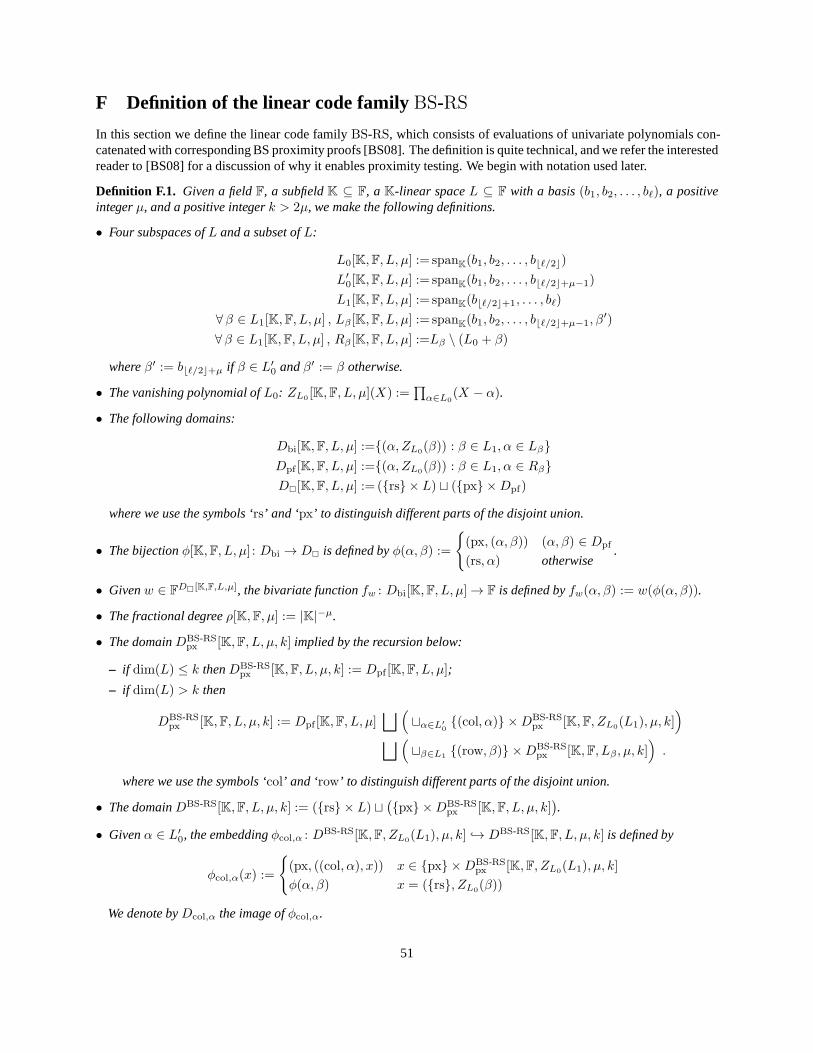
F Definition of the linear code familyBS-RS
In this section we define the linear code familyBS-RS, which consists of evaluations of univariate polynomials con-catenated with corresponding BS proximity proofs [BS08]. The definition is quite technical, and we refer the interestedreader to [BS08] for a discussion of why it enables proximitytesting. We begin with notation used later.
Definition F.1. Given a fieldF, a subfieldK ⊆ F, a K-linear spaceL ⊆ F with a basis(b1, b2, . . . , bℓ), a positiveintegerµ, and a positive integerk > 2µ, we make the following definitions.
• Four subspaces ofL and a subset ofL:
L0[K,F, L, µ] := spanK(b1, b2, . . . , b⌊ℓ/2⌋)
L′0[K,F, L, µ] := spanK(b1, b2, . . . , b⌊ℓ/2⌋+µ−1)
L1[K,F, L, µ] := spanK(b⌊ℓ/2⌋+1, . . . , bℓ)
∀β ∈ L1[K,F, L, µ] , Lβ[K,F, L, µ] := spanK(b1, b2, . . . , b⌊ℓ/2⌋+µ−1, β
′)
∀β ∈ L1[K,F, L, µ] , Rβ [K,F, L, µ] :=Lβ \ (L0 + β)
whereβ′ := b⌊ℓ/2⌋+µ if β ∈ L′0 andβ′ := β otherwise.
• The vanishing polynomial ofL0: ZL0 [K,F, L, µ](X) :=∏
α∈L0(X − α).
• The following domains:
Dbi[K,F, L, µ] :=(α,ZL0(β)) : β ∈ L1, α ∈ LβDpf [K,F, L, µ] :=(α,ZL0(β)) : β ∈ L1, α ∈ RβD[K,F, L, µ] := (rs × L) ⊔ (px ×Dpf)
where we use the symbols ‘rs’ and ‘px’ to distinguish different parts of the disjoint union.
• The bijectionφ[K,F, L, µ] : Dbi → D is defined byφ(α, β) :=
(px, (α, β)) (α, β) ∈ Dpf
(rs, α) otherwise.
• Givenw ∈ FD[K,F,L,µ], the bivariate functionfw : Dbi[K,F, L, µ]→ F is defined byfw(α, β) := w(φ(α, β)).
• The fractional degreeρ[K,F, µ] := |K|−µ.
• The domainDBS-RSpx [K,F, L, µ, k] implied by the recursion below:
– if dim(L) ≤ k thenDBS-RSpx [K,F, L, µ, k] := Dpf [K,F, L, µ];
– if dim(L) > k then
DBS-RSpx [K,F, L, µ, k] := Dpf [K,F, L, µ]
⊔
(
⊔α∈L′0(col, α) ×DBS-RS
px [K,F, ZL0(L1), µ, k])
⊔
(
⊔β∈L1 (row, β) ×DBS-RSpx [K,F, Lβ, µ, k]
)
.
where we use the symbols ‘col’ and ‘row’ to distinguish different parts of the disjoint union.
• The domainDBS-RS[K,F, L, µ, k] := (rs × L) ⊔(
px ×DBS-RSpx [K,F, L, µ, k]
)
.
• Givenα ∈ L′0, the embeddingφcol,α : DBS-RS[K,F, ZL0(L1), µ, k] → DBS-RS[K,F, L, µ, k] is defined by
φcol,α(x) :=
(px, ((col, α), x)) x ∈ px ×DBS-RSpx [K,F, ZL0(L1), µ, k]
φ(α, β) x = (rs, ZL0(β))
We denote byDcol,α the image ofφcol,α.
51

• Givenβ ∈ L1, the embeddingφrow,β : DBS-RS[K,F, Lβ, µ, k] → DBS-RS[K,F, L, µ, k] is defined by
φrow,β(x) :=
(px, ((row, β), x)) x ∈ px ×DBS-RSpx [K,F, Lβ, µ, k]
φ(α, β) x = (rs, α)We denote byDrow,β the image ofφrow,β.
• Givenα ∈ L′0, ψcol,α : FDBS-RS[K,F,L,µ,k] → F
DBS-RS[K,F,ZL0(L1),µ,k] is the projection ofDBS-RS[K,F, L, µ, k] onDcol,α with indices renamed to elements ofDBS-RS[K,F, ZL0(L1), µ, k]. Formally,ψcol,α(w) = w′ if and only ifw′(φcol,α(x)) = w(x) for all x ∈ DBS-RS[K,F, ZL0(L1), µ, k].
• Givenβ ∈ L1, ψrow,β : FDBS-RS[K,F,L,µ,k] → F
DBS-RS[K,F,Lβ,µ,k] is the projection ofDBS-RS[K,F, L, µ, k] onDrow,β with indices renamed to elements ofDBS-RS[K,F, Lβ, µ, k]. Formally, ψrow,β(w) = w′ if and only ifw′(φrow,β(x)) = w(x) for all x ∈ DBS-RS[K,F, Lβ, µ, k].
The following definition considers a code that extends the evaluation of a univariate polynomial with a bivariatefunction that represents the polynomial over a specially-chosen set.
Definition F.2 (RS). Given a fieldF, a subfieldK ⊆ F, aK-linear spaceL ⊆ F, and a positive integerµ, the codeRS[K,F, L, µ] consists of allw ∈ F
D[K,F,L,µ] such thatfw : Dbi → F is an evaluation of a low degree polynomial:there exists a polynomialg ∈ F[X,Y ] such that: (i)degX(g) < |L0|, (ii) degY (g) < |L1| ·ρ[K,F, µ], (iii) g|Dbi
= fw.
Ben-Sasson and Sudhan [BS08] show that:
• v ∈ RS[F, L, |L| · ρ] if and only if there existsw ∈ RS[K,F, L, µ] such thatw|rs×L = v;
• w ∈ RS[K,F, L, µ] if and only if
– for everyα ∈ L′0, fw|α×ZL0 (L1) ∈ RS[F, ZL0(L1), |L1| ·ρ] (with the standard mapping between domains) and– for everyβ ∈ L1, fw|Lβ×ZL0(β)
∈ RS[F, Lβ, |L0|] (with the standard mapping between domains).
The above equivalences illustrate the ‘quadratic reduction’ from testing thatw ∈ FL is a codeword ofRS[F, L, |L| · ρ]
to a set ofΘ(√
|L|) problems of testing membership in codes of the formRS[F, L′, d′] with |L′|, d′ = Θ(√
|L|).The code from Definition F.2 corresponds to one step of the recursive construction of [BS08]. We now build on
that definition, and recursively define the linear code family BS-RS.
Definition F.3 (BS-RS). Given a fieldF, a subfieldK ⊆ F, a K-linear spaceL ⊆ F, a positive integerµ, and apositive integerk > 2µ, the codeBS-RS[K,F, L, µ, k] consists of all wordsw ∈ F
DBS-RS[K,F,L,µ,k] satisfying thefollowing. If dim(L) ≤ k thenw ∈ RS[K,F, L, µ]. If dim(L) > k the following holds: (1) for everyα ∈ L′0 thereexistswα ∈ BS-RS[K,F, ZL0(L1), µ, k] such thatwα(φcol,α(x)) = w(x) for everyx ∈ D[K,F, ZL0(L1), µ, k];(2) for everyβ ∈ L1 there existswβ ∈ BS-RS[K,F, Lβ, µ, k] such thatwβ(φrow,β(x)) = w(x) for everyx ∈D[K,F, Lβ, µ, k].
We conclude this section with two claims aboutBS-RS that we use in later sections. We omit the proof of the firstclaim (and refer the interested reader to [BS08]), and provethe second claim based on the first one.
Claim F.4. For every codewordw ∈ RS[F, L, |L| · ρ], positive integerµ, and positive integerk > 2µ, there exists auniqueπw such thatw πw ∈ BS-RS[K,F, L, µ, k].
Claim F.5. The following two statements hold for the codeBS-RS[K,F, L, µ, k]:• for everyα ∈ L′0 andw′ ∈ BS-RS[K,F, ZL0(L1), µ, k] there existsw ∈ BS-RS[K,F, L, µ, k] such thatψcol,α(w) = w′;• for everyβ ∈ L1 andw′ ∈ BS-RS[K,F, Lβ, µ, k] there existsw ∈ BS-RS[K,F, L, µ, k] such thatψrow,β(w) = w′.
Proof. The proofs for the two statements are similar, so we only givethe proof for the first statement. Letw′ ∈BS-RS[K,F, ZL0(L1), µ, k], and definewrs := w′|rs×ZL0(L1); observe thatwrs in RS[F, ZL0(L1), |L1| · ρ]. ByClaim F.4,w′ is uniquely determined bywrs, thus it suffices to show that there existsw ∈ RS[K,F, L, µ] such thatfw|α×ZL0 (L1) = wrs. By definition ofRS, it suffices to show that there exists a bivariate polynomialg ∈ F[X,Y ]
such that: (i)degX(g) < |L0|, (ii) degY (g) < |L1| · ρ, (iii) g|α×ZL0(L1) = wrs ∈ RS[F, ZL0(L1), |L1| · ρ]. Theexistence of suchg follows by considering a suitable interpolating set (see, e.g., Appendix H).
52

G Proof of Lemma 4.27
In this section we prove Lemma 4.27. In Appendix G.1 we define the recursive cover and prove its combinatorial prop-erties; in Appendix G.2 we prove that a spanning set for the duals of codes in this cover can be computed efficiently;in Appendix G.3, we put these together to conclude the proof.
G.1 The recursive cover and its combinatorial properties
We define a recursive cover forBS-RS and then prove certain combinatorial properties for it. Thedefinition relies onthe definition of another cover, which we now introduce.
Definition G.1. Thenative coverS[K,F, L, µ, k] of BS-RS[K,F, L, µ, k] is defined as follows:
• if dim(L) ≤ k then the cover contains only the trivial view(DBS-RS[K,F, L, µ, k],BS-RS[K,F, L, µ, k]);
• if dim(L) > k then the cover contains
– the view(BS-RS[K,F, ZL0(L1), µ, k], Dcol,α) for everyα ∈ L′0, and– the view(BS-RS[K,F, Lβ, µ, k], Drow,β) for everyβ ∈ L1.
We now prove that the native cover is indeed a cover.
Claim G.2. The native cover ofBS-RS[K,F, L, µ, k] is a code cover (see Definition 4.13).
Proof. From Claim F.5 we know that:• for everyα ∈ L′0, the restriction ofBS-RS[K,F, L, µ, k] toDcol,α equalsBS-RS[K,F, ZL0(L1), µ, k];• for everyβ ∈ L1, the restriction ofBS-RS[K,F, L, µ, k] toDrow,β equalsBS-RS[K,F, Lβ, µ, k].Therefore, it suffices to show thatD ⊆ (∪α∈L′
0Dcol,α) ∪ (∪β∈L1Drow,β). So letx be an index inD.
• If there existsα ∈ L′0 such thatx ∈ px × (col, α) ×DBS-RSpf [K,F, ZL0(L1), µ, k], thenx ∈ Dcol,α.
• If there existsβ ∈ L1 such thatx ∈ px × (row, β) ×DBS-RSpf [K,F, Lβ, µ, k], thenx ∈ Drow,β .
• If x ∈ px×Dpf [K,F, L, µ], then there existβ ∈ L1 andα ∈ Rβ such thatx = (px, (α,ZL0(β))), sox ∈ Drow,β .• If x ∈ rs × L, then there existβ ∈ L1 andα ∈ Lβ such thatφ[K,F, L, µ](α,ZL0(β)) = x, sox ∈ Drow,β.
The recursive cover ofBS-RS is recursively defined based on the native cover ofBS-RS.
Definition G.3. The recursive coverT [K,F, L, µ, k]ofBS-RS[K,F, L, µ, k] is the tree of depth⌊log dim(L)− log(k)⌋where, for every non-leaf vertexv labeled by(D,BS-RS[K,F, L, µ, k]), the vertexv has|S[K,F, L, µ, k]| successors,all labeled by elements ofS[K,F, L, µ, k] with the natural embedding of their domains intoD.
Claim G.4. The recursive cover ofBS-RS[K,F, L, µ, k] is 1-intersecting (see Definition 4.18).
Proof. We must show that for every two disconnected verticesu, v it holds that|Du ∩ Dv| ≤ 1. It suffices to do sofor every two distinctsiblingsu, v, because ifa is an ancestor ofb thenDa containsDb. Hence, we only need to showthat for every two distinct views(D, C), (D′, C′) in the native coverS[K,F, L, µ, k], it holds that|D ∩ D′| ≤ 1. Firstwe observe that for everyα1 6= α2 ∈ L′0 andβ1 6= β2 ∈ L1, the following sets are disjoint by definition:• px × (col, α1) ×DBS-RS
pf [K,F, ZL0(L1), µ, k],• px × (col, α2) ×DBS-RS
pf [K,F, ZL0(L1), µ, k],• px × (row, β1) ×DBS-RS
pf [K,F, Lβ1, µ, k],• px × (row, β2) ×DBS-RS
pf [K,F, Lβ2, µ, k].Thus it is enough to show that:• Any two columns are distinct:φ(α1, β1) 6= φ(α2, β2) for everyα1 6= α2 ∈ L′0 andβ1, β2 ∈ ZL0(L1).• Any two rows are distinct:φ(α1, β1) 6= φ(α2, β2) for everyβ1 6= β2 ∈ ZL0(L1), α1 ∈ Lβ1 , andα2 ∈ Lβ2 .• The intersection of any row and column has at most one element: φ(α, β′) 6= φ(α′, β) for everyα, α′ ∈ L′0 andβ, β′ ∈ ZL0(L1) with (α′, β′) 6= (α, β).
But all the above follow from the fact thatφ[K,F, L, µ] is a bijection and, thus, an injection.
53

The next claim establishes a connection between the depth ofa vertexv in the recursive cover and the independenceof the coverTv of the codeCv.
Claim G.5. For every vertexv in layer(T, d), the coverTv is (|K|dim(L)·2−d−1−µ−2)-independent. In particular, byassignment, it holds that, for every positive integerm and every non-leaf vertexv in T [K,F, L, µ, k] with depth lessthanlog2 dim(L)− log2(log|K|m+ µ+ 2)− 1, the coverTv ism-independent.
The proof of the above claim directly follows from Claim G.7 and Claim G.6, stated and proved below. The first ofthese two claims connects the depth of a vertexv and the dimension of a spaceLv such thatCv = BS-RS[F,K, Lv, µ, k](this claim is used separately also for establishing computational properties in in Appendix G.2).
Claim G.6. If v ∈ layer(T [K,F, L, µ, k], d) thenCv = BS-RS[K,F, L, µ, k] for someL such that
dim(L) · 2−d ≤ dim(L) ≤ dim(L) · 2−d + 2µ .
Proof. The proof is by induction ond. The base cased = 0 follows directly from the definition; so we now assumethe claim ford − 1 and prove it ford. Let v ∈ layer(T, d) be a vertex of depthd, and letu ∈ layer(T, d− 1) bev’spredecessor. By the inductive assumption,Cu = BS-RS[K,F, Lu, µ, k] for someLu such thatdim(L) · 2−(d−1) ≤dim(Lu) ≤ dim(L) · 2−(d−1) + 2µ.
First we argue thatTu is not the trivial (singleton) cover. For this, it suffices toshow thatdim(Lu) > k. But thisfollows from the inductive assumption, sincedepth(T, u) < ⌊log dim(L)− log(k)⌋, so thatdim(Lu) ≥ dim(L) ·2−(⌊log dim(L)−log(k)⌋−1) ≥ 2k.
RecallCv = BS-RS[K,F, Lv, µ, k] for some spaceLv; we are thus left to show thatdim(Lu) ·2−1 ≤ dim(Lv) ≤dim(Lu)·2−1+µ. We do so by giving two cases, based on the form ofLv: (a) ifLv = ZL0[K,F,Lu,µ,k](L1[K,F, Lu, µ, k])
thendim(Lv) = dim(L1[K,F, Lu, µ, k]) = ⌈dim(Lu)2 ⌉; (b) if there existsβ ∈ L1[K,F, Lu, µ, k] such thatLv =
Lβ[K,F, Lu, µ, k] thendim(Lv) = dim(L0[K,F, Lu, µ, k]) + µ = ⌊dim(Lu)2 ⌋ + µ. In either casedim(Lu) · 2−1 ≤
dim(Lv) ≤ dim(Lu) · 2−1 + µ, and the claim follows.
Claim G.7. The native coverS[K,F, L, µ, k] is |K| dim(L)2 −µ−2-independent.
Proof. Recalling Definition 4.16, fix arbitrary subsetsD′ ⊆ (col × L′0) ⊔ (row × L1) andD′′ ⊆ D[K,F, L, µ]
both of size at most|K| dim(L)2 −µ−2, and defineD := D′′ ∪ (∪(col,α)∈D′Dcol,α) ∪ (∪(row,β)∈D′Drow,β). Let w′ ∈
FDBS-RS
be such that: (i) for every(col, α) ∈ D′ it holds thatψcol,α(w′) ∈ BS-RS[K,F, ZL0(L1), µ, k]; and (ii) for
every (row, β) ∈ D′ it holds thatψrow,β(w′) ∈ BS-RS[K,F, Lβ, µ, k]. We need to show that there existsw ∈
BS-RS[K,F, L, µ, k] such thatw|D = w′|D.In fact, it suffices to show that there existsw ∈ RS[K,F, L, µ] such thatw|D∩D
= w′|D∩D, because
Claim F.4 implies there exists a unique codewordw ∈ BS-RS[K,F, L, µ, k] such thatw|D= w andw|D = w′|D.
Thus, we now argue that there existsw ∈ RS[K,F, L, µ] such that the following holds.
• For every(col, α) ∈ D′ andβ ∈ ZL0(L1), it holds thatfw(α, β) = w′(φ(α, β)) = (ψcol,α(w
′)) (rs, β). Inparticular,fw
|α×ZL0 (L1) ∈ RS[F, ZL0(L1), |L1| · ρ], and letpcol,α be its univariate low degree extension toF.
• For every(row, β) ∈ D′ andα ∈ Lβ, it holds thatfw(α,ZL0(β)) = w′(φ(α,ZL0 (β))) = (ψrow,β(w
′)) (rs, α).In particular,fw
|Lβ×ZL0(L1) ∈ RS[F, Lβ, |L0|], and letprow,β be its univariate low degree extension toF.
• For every(α, β) ∈ D′′, it holds thatfw(α,ZL0(β)) = w′(φ(α,ZL0 (β))).
By Definition F.2 it suffices to show that there exists a bivariate polynomialg ∈ F[X,Y ] such that: (i)degX(g) < |L0|;(ii) degY (g) < |L1| · ρ; (iii) g|X=α = pcol,α for every(col, α) ∈ D′; (iv) g|Y=ZL0 (β)
= prow,β for every(row, β) ∈D′; (v) g(α, β) = w′(φ(α,ZL0(β))) for every(α, β) ∈ D′′. But notice that|D′| + |D′′| ≤ 2 · |K| dim(L)
2 −µ−2 =
|K| dim(L)2 −µ−1 < min|L0|, |L1| · ρ, because (a)log|K|(|L0|) = dim(L0) ≥ dim(L)
2 − 1, and (b)log|K|(|L1| · ρ) =dim(L1)− µ ≥ dim(L)
2 − µ. The claim follows by considering a suitable interpolatingset (see Section H).
54
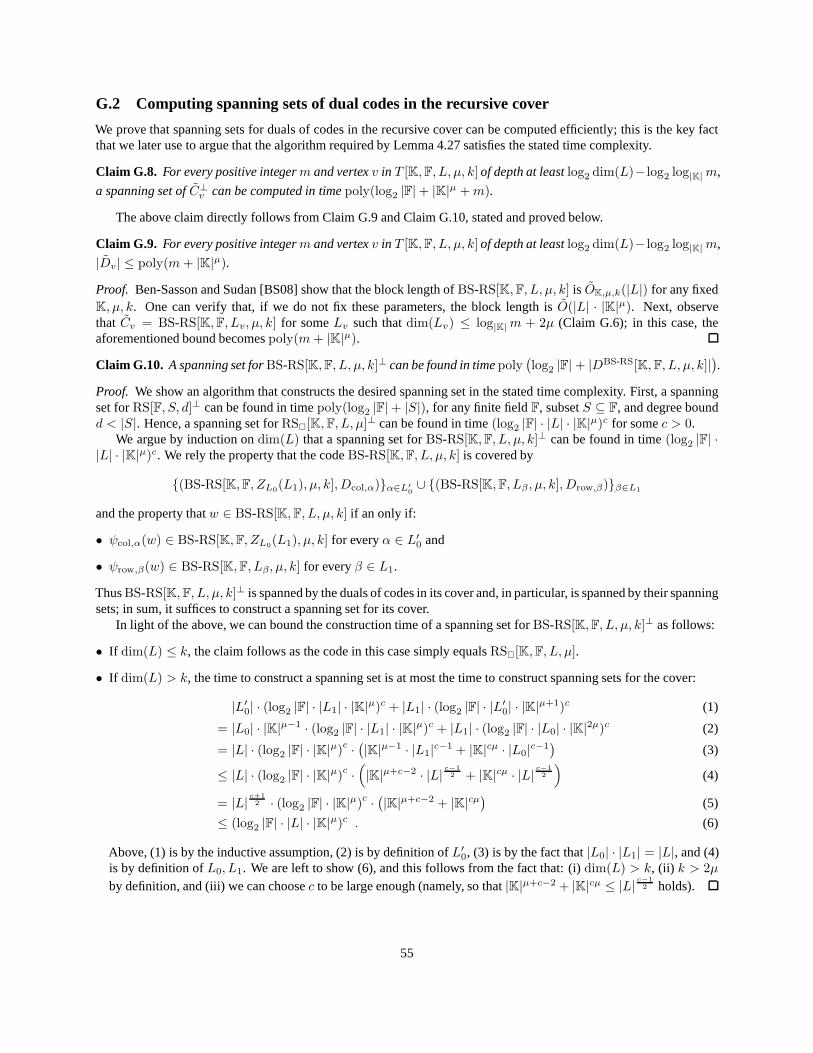
G.2 Computing spanning sets of dual codes in the recursive cover
We prove that spanning sets for duals of codes in the recursive cover can be computed efficiently; this is the key factthat we later use to argue that the algorithm required by Lemma 4.27 satisfies the stated time complexity.
Claim G.8. For every positive integerm and vertexv in T [K,F, L, µ, k] of depth at leastlog2 dim(L)− log2 log|K|m,
a spanning set ofC⊥v can be computed in timepoly(log2 |F|+ |K|µ +m).
The above claim directly follows from Claim G.9 and Claim G.10, stated and proved below.
Claim G.9. For every positive integerm and vertexv in T [K,F, L, µ, k] of depth at leastlog2 dim(L)− log2 log|K|m,
|Dv| ≤ poly(m+ |K|µ).
Proof. Ben-Sasson and Sudan [BS08] show that the block length ofBS-RS[K,F, L, µ, k] is OK,µ,k(|L|) for any fixedK, µ, k. One can verify that, if we do not fix these parameters, the block length isO(|L| · |K|µ). Next, observethat Cv = BS-RS[K,F, Lv, µ, k] for someLv such thatdim(Lv) ≤ log|K|m + 2µ (Claim G.6); in this case, theaforementioned bound becomespoly(m+ |K|µ).
Claim G.10. A spanning set forBS-RS[K,F, L, µ, k]⊥ can be found in timepoly(
log2 |F|+ |DBS-RS[K,F, L, µ, k]|)
.
Proof. We show an algorithm that constructs the desired spanning set in the stated time complexity. First, a spanningset forRS[F, S, d]⊥ can be found in timepoly(log2 |F|+ |S|), for any finite fieldF, subsetS ⊆ F, and degree boundd < |S|. Hence, a spanning set forRS[K,F, L, µ]
⊥ can be found in time(log2 |F| · |L| · |K|µ)c for somec > 0.We argue by induction ondim(L) that a spanning set forBS-RS[K,F, L, µ, k]⊥ can be found in time(log2 |F| ·
|L| · |K|µ)c. We rely the property that the codeBS-RS[K,F, L, µ, k] is covered by
(BS-RS[K,F, ZL0(L1), µ, k], Dcol,α)α∈L′0∪ (BS-RS[K,F, Lβ, µ, k], Drow,β)β∈L1
and the property thatw ∈ BS-RS[K,F, L, µ, k] if an only if:
• ψcol,α(w) ∈ BS-RS[K,F, ZL0(L1), µ, k] for everyα ∈ L′0 and
• ψrow,β(w) ∈ BS-RS[K,F, Lβ, µ, k] for everyβ ∈ L1.
ThusBS-RS[K,F, L, µ, k]⊥ is spanned by the duals of codes in its cover and, in particular, is spanned by their spanningsets; in sum, it suffices to construct a spanning set for its cover.
In light of the above, we can bound the construction time of a spanning set forBS-RS[K,F, L, µ, k]⊥ as follows:
• If dim(L) ≤ k, the claim follows as the code in this case simply equalsRS[K,F, L, µ].
• If dim(L) > k, the time to construct a spanning set is at most the time to construct spanning sets for the cover:
|L′0| · (log2 |F| · |L1| · |K|µ)c + |L1| · (log2 |F| · |L′0| · |K|µ+1)c (1)
= |L0| · |K|µ−1 · (log2 |F| · |L1| · |K|µ)c + |L1| · (log2 |F| · |L0| · |K|2µ)c (2)
= |L| · (log2 |F| · |K|µ)c ·(
|K|µ−1 · |L1|c−1 + |K|cµ · |L0|c−1)
(3)
≤ |L| · (log2 |F| · |K|µ)c ·(
|K|µ+c−2 · |L| c−12 + |K|cµ · |L| c−1
2
)
(4)
= |L| c+12 · (log2 |F| · |K|µ)c ·
(
|K|µ+c−2 + |K|cµ)
(5)
≤ (log2 |F| · |L| · |K|µ)c . (6)
Above, (1) is by the inductive assumption, (2) is by definition ofL′0, (3) is by the fact that|L0| · |L1| = |L|, and (4)is by definition ofL0, L1. We are left to show (6), and this follows from the fact that: (i) dim(L) > k, (ii) k > 2µ
by definition, and (iii) we can choosec to be large enough (namely, so that|K|µ+c−2 + |K|cµ ≤ |L| c−12 holds).
55

G.3 Putting things together
Proof of Lemma 4.27.Define the depth functiond(K, L, µ, a) := log2 dim(L) − log2(log|K| a + µ + 2) − 1. Weargue the two conditions in the lemma. First, for every indexn = (K,F, L, µ, k), T [K,F, L, µ, k] is a1-intersectingrecursive cover ofBS-RS[K,F, L, µ, k] (by Claim G.4). Moreover, for every positive integerm and non-leaf vertexvin T with depth(T, v) < d(K, L, µ,m), the coverTv ism-independent (by Claim G.5).
Second, consider the algorithm that, given an indexn = (K,F, L, µ, k) and subsetI ⊆ DBS-RS[K,F, L, µ, k],works as follows: (1) for everyα ∈ I choose an arbitrary vertexvα in layer(T, d(K, L, µ, |I|)) such thatα ∈ Dvα ,and then setU := vαα∈I ; (2) compute a spanning setWv set forC⊥v ; (3) returnW := ∪u∈UWu. This algorithmsatisfies the required properties. First, it runs in timepoly(log2 |F|+dim(L)+|K|µ+|I|) because a spanning set set forC⊥u can be computed in timepoly(log2 |F|+ |K|µ + |I|) (by Claim G.8). Next, its outputW meets the requirements:• U ⊆ layer(T [K,F, L, µ, k], d(K, L, µ, |I|));• |U | ≤ |I|, by definition ofU ;• I ⊆ (∪u∈U Du), by definition ofU ;• span(W ) = span(∪u∈UWu) = span(∪u∈U C⊥u ), by definition ofW andWu.This completes the proof of Lemma 4.27.
56
H Folklore claim on interpolating sets
Claim H.1. LetF be a field, letdcols, drows ∈ N, and consider three setsScols, Srows ⊆ F andSpnts ⊆ F× F such that|Scols|+ |Srows|+ |Spnts| ≤ mindcols, drows. Letf : F× F→ F be a function such that:
• for everyα ∈ Scols there existsgcol,α ∈ F<drows [x] such thatf(α, β) = gcol,α(β) for everyβ ∈ F;
• for everyβ ∈ Srows there existsgrow,β ∈ F<dcols [x] such thatf(α, β) = grow,β(α) for everyα ∈ F.
Then there existsg ∈ F[X,Y ] such that: (i)degX(g) < drows; (ii) degY (g) < dcols; (iii) g|X=α = gcol,α for everyα ∈ Scols; (iv) g|Y=β = grow,β for everyβ ∈ Srows; (v) g(α, β) = f(α, β) for every(α, β) ∈ Spnts.
Proof. Any rectangleDX ×DY ⊆ F× F with |DX | = drows and|DY | = dcols is an interpolating set: for everyw ∈FDX×DY there exists a uniqueg ∈ F[X,Y ] such that: (i)degX(g) < drows; (ii) degY (g) < dcols; (iii) g|DX×DY
= w.Define
DX := Scols ∪ α : ∃β s.t. (α, β) ∈ Spnts and DY := Srows ∪ β : ∃α s.t. (α, β) ∈ Spnts .
Note that|DX | ≤ drows and|DY | ≤ dcols; if either is strictly smaller, extend it arbitrarily to match the upper bound.Choosew ∈ F
DX×DY to be a word that satisfies: (i)w(α, β) = f(α, β) for everyα ∈ Scols andβ ∈ DY ;(ii) w(α, β) = f(α, β) for everyβ ∈ Srows andα ∈ DX ; (iii) w(α, β) = f(α, β) for every(α, β) ∈ Spnts. Denote bygw ∈ F[X,Y ] the unique “low degree extension” ofw; we show thatgw satisfies the requirements of the claim.
The degree bounds and the equivalence onSpnts follows by definition ofgw; thus it suffices to show equivalenceof gw with f when restricted to the required rows and columns.
• For everyα ∈ Scols: it holds by definition ofgw thatgw|α×DY= f |α×DY
; moreover,gw|α×F andf |α×Fare evaluations of polynomials of degree less than|DY |, which implies thatgw|α×F = f |α×F.
• For everyβ ∈ Srows: it holds by definition ofgw thatgw|DX×β = f |DX×β; moreover,gw|F×β andf |F×βare evaluations of polynomials of degree less than|DX |, which implies thatgw|F×β = f |F×β.
57

References[AH91] William Aiello and Johan Hastad. Statistical zero-knowledge languages can be recognized in two rounds.Journal of
Computer and System Sciences, 42(3):327–345, 1991. Preliminary version appeared in FOCS ’87.
[ALM +98] Sanjeev Arora, Carsten Lund, Rajeev Motwani, Madhu Sudan, and Mario Szegedy. Proof verification and the hardnessof approximation problems.Journal of the ACM, 45(3):501–555, 1998. Preliminary version in FOCS ’92.
[AS98] Sanjeev Arora and Shmuel Safra. Probabilistic checking of proofs: a new characterization of NP.Journal of the ACM,45(1):70–122, 1998. Preliminary version in FOCS ’92.
[AS03] Sanjeev Arora and Madhu Sudan. Improved low-degree testing and its applications.Combinatorica, 23(3):365–426,2003. Preliminary version appeared in STOC ’97.
[Bab85] Laszlo Babai. Trading group theory for randomness. InProceedings of the 17th Annual ACM Symposium on Theoryof Computing, STOC ’85, pages 421–429, 1985.
[BCG+16] Eli Ben-Sasson, Alessandro Chiesa, Ariel Gabizon, Michael Riabzev, and Nicholas Spooner. Short interactive oracleproofs with constant query complexity, via composition andsumcheck, 2016. Crypto ePrint 2016/324.
[BCGV16] Eli Ben-Sasson, Alessandro Chiesa, Ariel Gabizon, and Madars Virza. Quasilinear-size zero knowledge from linear-algebraic PCPs. InProceedings of the 13th Theory of Cryptography Conference, TCC ’16-A, pages 33–64, 2016.
[BCS16] Eli Ben-Sasson, Alessandro Chiesa, and Nicholas Spooner. Interactive oracle proofs. InProceedings of the 14thTheory of Cryptography Conference, TCC ’16-B, pages ??–??, 2016.
[BFL91] Laszlo Babai, Lance Fortnow, and Carsten Lund. Non-deterministic exponential time has two-prover interactiveprotocols.Computational Complexity, 1:3–40, 1991. Preliminary version appeared in FOCS ’90.
[BFLS91] Laszlo Babai, Lance Fortnow, Leonid A. Levin, and Mario Szegedy. Checking computations in polylogarithmictime.In Proceedings of the 23rd Annual ACM Symposium on Theory of Computing, STOC ’91, pages 21–32, 1991.
[BGG+88] Michael Ben-Or, Oded Goldreich, Shafi Goldwasser, JohanHastad, Joe Kilian, Silvio Micali, and Phillip Rogaway.Everything provable is provable in zero-knowledge. InProceedings of the 8th Annual International Cryptology Con-ference, CRYPTO ’89, pages 37–56, 1988.
[BGH+06] Eli Ben-Sasson, Oded Goldreich, Prahladh Harsha, MadhuSudan, and Salil P. Vadhan. Robust PCPs of proximity,shorter PCPs, and applications to coding.SIAM Journal on Computing, 36(4):889–974, 2006.
[BGK+10] Eli Ben-Sasson, Venkatesan Guruswami, Tali Kaufman, Madhu Sudan, and Michael Viderman. Locally testable codesrequire redundant testers.SIAM Journal on Computing, 39(7):3230–3247, 2010.
[BGKW88] Michael Ben-Or, Shafi Goldwasser, Joe Kilian, and Avi Wigderson. Multi-prover interactive proofs: how to removeintractability assumptions. InProceedings of the 20th Annual ACM Symposium on Theory of Computing, STOC ’88,pages 113–131, 1988.
[BHR05] Eli Ben-Sasson, Prahladh Harsha, and Sofya Raskhodnikova. Some 3CNF properties are hard to test.SIAM Journalon Computing, 35(1):1–21, 2005.
[BHZ87] Ravi B. Boppana, Johan Hastad, and Stathis Zachos.Does co-NP have short interactive proofs?Information Process-ing Letters, 25(2):127–132, 1987.
[BM88] Laszlo Babai and Shlomo Moran. Arthur-merlin games: A randomized proof system, and a hierarchy of complexityclasses.Journal of Computer and System Sciences, 36(2):254–276, 1988.
[BS08] Eli Ben-Sasson and Madhu Sudan. Short PCPs with polylog query complexity. SIAM Journal on Computing,38(2):551–607, 2008. Preliminary version appeared in STOC’05.
[BVW98] Ronald V. Book, Heribert Vollmer, and Klaus W. Wagner. Probabilistic type-2 operators and “almost”-classes.Com-putational Complexity, 7(3):265–289, 1998.
[BW04] Andrej Bogdanov and Hoeteck Wee. A stateful implementation of a random function supporting parity queries over hy-percubes. InProceedings of the 7th International Workshop on Approximation Algorithms for Combinatorial Optimiza-tion Problems, and of the 8th International Workshop on Randomization and Computation, APPROX-RANDOM ’04,pages 298–309, 2004.
[DFK+92] Cynthia Dwork, Uriel Feige, Joe Kilian, Moni Naor, and Shmuel Safra. Low communication 2-prover zero-knowledgeproofs for NP. InProceedings of the 11th Annual International Cryptology Conference, CRYPTO ’92, pages 215–227,1992.
58
[DR04] Irit Dinur and Omer Reingold. Assignment testers: Towards a combinatorial proof of the PCP theorem. InProceedingsof the 45th Annual IEEE Symposium on Foundations of ComputerScience, FOCS ’04, pages 155–164, 2004.
[DS98] Cynthia Dwork and Amit Sahai. Concurrent zero-knowledge: Reducing the need for timing constraints. InProceed-ings of the 18th Annual International Cryptology Conference, CRYPTO ’98, pages 442–457, 1998.
[FGL+96] Uriel Feige, Shafi Goldwasser, Laszlo Lovasz, Shmuel Safra, and Mario Szegedy. Interactive proofs and the hardnessof approximating cliques.Journal of the ACM, 43(2):268–292, 1996. Preliminary version in FOCS ’91.
[For87] Lance Fortnow. The complexity of perfect zero-knowledge (extended abstract). InProceedings of the 19th AnnualACM Symposium on Theory of Computing, STOC ’87, pages 204–209, 1987.
[FRS88] Lance Fortnow, John Rompel, and Michael Sipser. On the power of multi-prover interactive protocols. InTheoreticalComputer Science, pages 156–161, 1988.
[FS89] Uriel Feige and Adi Shamir. Zero knowledge proofs of knowledge in two rounds. InProceedings of the 9th AnnualInternational Cryptology Conference, CRYPTO ’89, pages 526–544, 1989.
[GGN10] Oded Goldreich, Shafi Goldwasser, and Asaf Nussboim. On the implementation of huge random objects.SIAMJournal on Computing, 39(7):2761–2822, 2010. Preliminary version appeared in FOCS ’03.
[GIMS10] Vipul Goyal, Yuval Ishai, Mohammad Mahmoody, and Amit Sahai. Interactive locking, zero-knowledge PCPs, andunconditional cryptography. InProceedings of the 30th Annual Conference on Advances in Cryptology, CRYPTO’10,pages 173–190, 2010.
[GKR08] Shafi Goldwasser, Yael Tauman Kalai, and Guy N. Rothblum. Delegating computation: Interactive proofs for Muggles.In Proceedings of the 40th Annual ACM Symposium on Theory of Computing, STOC ’08, pages 113–122, 2008.
[GMR89] Shafi Goldwasser, Silvio Micali, and Charles Rackoff. The knowledge complexity of interactive proof systems.SIAMJournal on Computing, 18(1):186–208, 1989. Preliminary version appeared in STOC ’85.
[GO94] Oded Goldreich and Yair Oren. Definitions and properties of zero-knowledge proof systems.Journal of Cryptology,7(1):1–32, December 1994.
[GR15] Tom Gur and Ron D. Rothblum. Non-interactive proofs of proximity. In Proceedings of the 6th Innovations inTheoretical Computer Science Conference, ITCS ’15, pages 133–142, 2015.
[GS06] Oded Goldreich and Madhu Sudan. Locally testable codes and PCPs of almost-linear length.Journal of the ACM,53:558–655, July 2006. Preliminary version in STOC ’02.
[IMS12] Yuval Ishai, Mohammad Mahmoody, and Amit Sahai. On efficient zero-knowledge PCPs. InProceedings of the 9thTheory of Cryptography Conference on Theory of Cryptography, TCC ’12, pages 151–168, 2012.
[IMSX15] Yuval Ishai, Mohammad Mahmoody, Amit Sahai, and David Xiao. On zero-knowledge PCPs: Limitations, simplifications, and applications, 2015. Available athttp://www.cs.virginia.edu/ ˜ mohammad/files/papers/ZKPCPs-Full.pdf .
[IW14] Yuval Ishai and Mor Weiss. Probabilistically checkable proofs of proximity with zero-knowledge. InProceedings ofthe 11th Theory of Cryptography Conference, TCC ’14, pages 121–145, 2014.
[IWY16] Yuval Ishai, Mor Weiss, and Guang Yang. Making the best of a leaky situation: Zero-knowledge PCPs from leakage-resilient circuits. InProceedings of the 13th Theory of Cryptography Conference, TCC ’16-A, pages 3–32, 2016.
[IY87] Russell Impagliazzo and Moti Yung. Direct minimum-knowledge computations. InProceedings of the 7th AnnualInternational Cryptology Conference, CRYPTO ’87, pages 40–51, 1987.
[Kay10] Neeraj Kayal. Algorithms for arithmetic circuits,2010. ECCC TR10-073.
[KI04] Valentine Kabanets and Russell Impagliazzo. Derandomizing polynomial identity tests means proving circuit lowerbounds.Computational Complexity, 13(1-2):1–46, 2004.
[KLR10] Eyal Kushilevitz, Yehuda Lindell, and Tal Rabin. Information-theoretically secure protocols and security under com-position.SIAM Journal on Computing, 39(5):2090–2112, 2010. Preliminary version appeared in STOC ’06.
[KPT97] Joe Kilian, Erez Petrank, and Gabor Tardos. Probabilistically checkable proofs with zero knowledge. InProceedingsof the 29th Annual ACM Symposium on Theory of Computing, STOC ’97, pages 496–505, 1997.
[KR08] Yael Kalai and Ran Raz. Interactive PCP. InProceedings of the 35th International Colloquium on Automata, Lan-guages and Programming, ICALP ’08, pages 536–547, 2008.
[LFKN92] Carsten Lund, Lance Fortnow, Howard J. Karloff, and Noam Nisan. Algebraic methods for interactive proof systems.Journal of the ACM, 39(4):859–868, 1992.
59

[LS95] Dror Lapidot and Adi Shamir. A one-round, two-prover, zero-knowledge protocol for NP.Combinatorica, 15(2):204–214, 1995.
[MX13] Mohammad Mahmoody and David Xiao. Languages with efficient zero-knowledge PCPs are in SZK. InProceedingsof the 10th Theory of Cryptography Conference, TCC ’13, pages 297–314, 2013.
[Nao91] Moni Naor. Bit commitment using pseudorandomness.Journal of Cryptology, 4(2):151–158, 1991. Preliminaryversion appeared in CRYPTO ’89.
[Nis93] Noam Nisan. On read-once vs. multiple access to randomness in logspace.Theoretical Computer Science, 107(1):135–144, 1993.
[Ost91] Rafail Ostrovsky. One-way functions, hard on average problems, and statistical zero-knowledge proofs. InProceed-ings of the 6th Annual Structure in Complexity Theory Conference, CoCo ’91, pages 133–138, 1991.
[OW93] Rafail Ostrovsky and Avi Wigderson. One-way functions are essential for non-trivial zero-knowledge. InProceedingsof the 2nd Israel Symposium on Theory of Computing Systems, ISTCS ’93, pages 3–17, 1993.
[RRR16] Omer Reingold, Ron Rothblum, and Guy Rothblum. Constant-round interactive proofs for delegating computation.In Proceedings of the 48th ACM Symposium on the Theory of Computing, STOC ’16, pages 49–62, 2016.
[RS96] Ronitt Rubinfeld and Madhu Sudan. Robust characterizations of polynomials with applications to program testing.SIAM Journal on Computing, 25(2):252–271, 1996.
[RS05] Ran Raz and Amir Shpilka. Deterministic polynomial identity testing in non-commutative models.ComputationalComplexity, 14(1):1–19, 2005. Preliminary version appeared in CCC ’04.
[Sch80] Jacob T. Schwartz. Fast probabilistic algorithms for verification of polynomial identities.Journal of the ACM,27(4):701–717, 1980.
[Sha92] Adi Shamir. IP = PSPACE.Journal of the ACM, 39(4):869–877, 1992.
[SY10] Amir Shpilka and Amir Yehudayoff. Arithmetic circuits: A survey of recent results and open questions.Foundationsand Trends in Theoretical Computer Science, 5(3-4):207–388, 2010.
[Zip79] Richard Zippel. Probabilistic algorithms for sparse polynomials. InProceedings of the 1979 International Symposiumon Symbolic and Algebraic Computation, EUROSAM ’79, pages 216–226, 1979.
60