on power-law relationships of the internet...

On Power-Law Relationships of the Internet Topology

Michalis Faloutsos Petros Faloutsos

U.C. Riverside U. of Toronto Dept. of Comp. Science Dept. of Comp. Science [email protected] [email protected]

Christos Faloutsos * Carnegie Mellon Univ.

Dept. of Comp. Science christosQcs.cmu.edu

Abstract

Despite the apparent randomness of the Internet, we dis- cover some surprisingly simple power-laws of the Internet topology. These power-laws hold for three snapshots of the Internet, between November 1997 and December 1998, despite a 45% growth of its size during that period. We show that our power-laws fit the real data very well resulting in correlation coefficients of 96% or higher.

Our observations provide a novel perspective of the structure of the Internet. The power-laws describe concisely skewed distributions of graph properties such as the node outdegree. In addition, these power-laws can be used to estimate important parameters such as the average neighborhood size, and facilitate the design and the performance analysis of protocols. Furthermore, we can use them to generate and select realistic topologies for simulation purposes.

1 Introduction

“What does the Internet look like?” “Are there any topological properties that don’t change in time?” ~‘How will it look like a year from now?” “How can I generate Internet-like graphs for my simulations?” These are some of the questions motivating this work.

In this paper, we study the topology of the Internet and we identify several power-laws. Furthermore, we discuss multiple benefits from understanding the topology of the Internet. First, we can design more efficient protocols that take advantage of its topological properties. Second, we can create more accurate artificial models for simulation purposes. And third, we can derive estimates for topological parameters (e.g. the average number of neighbors within h

*This research was partially funded by the National Science Foun- dation under Grants No. IRI-9625428 and DMS-9873442. Also, by the National Science Foundation, ARPA and NASA under NSF Co-

operative Agreement No. IRI-9411299, and by DARPA/ITO through Order F463, issued by ESC/ENS under contract N66001-97-C-851. Additional funding was provided by dooations from NEC and Intel. Views and conclusions contained in this document are those of the authors and should not be interpreted as representing official poli- cies, either expressed or implied, of the Defense Advanced Research Projects Agency or of the United States Government.

Permission to make digital or hard copies of all or part of this work for personal or classroom use is granted without fee provided that copies are not made or distributed for profit or commercial advantage and that copies bear this notice and the full citation on the first page. To copy otherwise, to republish, to post on servers or to redistribute to lists, requires prior specific permission and/or a fee. SIGCOMM ‘99 9199 Cambridge, MA, USA Q 1999 ACM l-58113-135.6/99/0008...$5.00

hops) that are useful for the analysis of protocols and for speculations of the Internet topolog in the future.

P. Modeling the Internet topology is an important open problem despite the attention it has attracted recently. Pax- son and Floyd consider this problem as a major reason “Why We Don’t Know How To Simulate The Internet” [16]. Sev- eral graph-generator models have been proposed [23] [5] [27], but the problem of creating realistic topologies is not yet solved; the selection of several parameter values are left to the intuition and the experience of each researcher.

As our primary contribution, we identify three power- laws for the topology of the Internet over the duration of a year in 1998. Power-laws are expressions of the form y 0: zQ, where a is a constant, z and y are the measures of interest, and o( stands for “proportional to”. Some of those exponents do not change significantly over time, while some exponents change by approximately 10%. However, the important observation is the existence of power-laws, i.e., the fact that there is some exponent for each graph instance. During 1998, these power-laws hold in three Internet instances with good linear fits in log-log plots; the correlation coefficient of the fit is at least 96% and usually higher than 98%. In addition, we introduce a graph metric to quantify the density of a graph and propose a rough power-law approximation of that metric. Furthermore, we show how to use our power- laws and our approximation to estimate useful parameters of the Internet, such as the average number of neighbors within h hops. Finally, we focus on the generation of realistic graphs. Our power-laws can help verify the realism of synthetic topologies. In addition, we measure several crucial parameters for the most recent graph generator [27].

Our work in perspective. Our work is based on three In- ternet instances over a one-year period. During this time, the size of the network increased substantially (45%). De- spite this, the sample space is rather limited, and mak- ing any generalizations would be premature until additional studies are conducted. However, the authors believe that these power-laws characterize the dynamic equilibrium of the Internet growth in the same way power-laws appear to describe various natural networks such as the the human respiratory system [12], and automobile networks [6]. At a more practical level, the regularities characterize the topology concisely during 1998. If this time period turns out to be a transition phase for the Internet, our observations will obviously be valid only for 1998. In absence of revolutionary

‘In this paper, we use the expression “the topology of the Inter- net”, although the topology changes and it would be more accurate to talk about “Internet topologies”. We hope that this does not mislead or confuse the reader.

251

changes, it is reasonable to expect that our power-laws will continue to hold in the future.

The rest of this paper is structured as follows. In Sec- tion 2, we present some definitions and previous work on measurements and models for the Internet. In Section 3, we present our Internet instances and provide useful measurements. In Section 4, we present our three observed power- laws and our power-law approximation. In Section 5, we explain the intuition behind our power-laws, discuss their use, and show how we can use them to predict the growth of the Internet. In Section 6, we conclude our work and discuss future directions.

2 Background and Previous Work

The Internet can be decomposed into connected subnetworks that are under separate administrative authorities, as shown in Figure 1. These subnetworks are called domains or autonomous systems’. This way, the topology of the Internet can be studied at two different granularities. At the router level, we represent each router by a node [14]. At the inter-domain level, each domain is represented by a single node [lo] and each edge is an inter-domain inter- connection. The study of the topology at both levels is equally important. The Internet community develops and employs different protocols inside a domain and between domains. An intra-domain protocol is limited within a domain, while an inter-domain protocol runs between domains treating each domain as one entity.

Symbol Definition

G An undirected graph.

N Number of nodes in a graph.

E Number of edges in a graph.

6 The diameter of the graph.

dv Outdegree of node u.

2 The average outdegree of the nodes of a 1 graph: 6=2 E/N -

Table 1: Definitions and symbols.

Metrics. The metrics that have been used so far to describe graphs are mainly the node outdegree, and the distances between nodes. Given a graph, the outdegree of a node is defined as the number of edges incident to the node (see Table 1). The distance between two nodes is the number of edges of the shortest path between the two nodes. Most studies report minimum, maximum, and average values and plot the outdegree and distance distribution. We denote the number of nodes of a graph by N, t.he number of edges by E, and the diameter of the graph by 6.

Real network studies. Govindan and Reddy [lo] study the growth of the inter-domain topology of the Internet between 1994 and 1995. The graph is sparse with 75% of the nodes having outdegrees less or equal to two. They distinguish four groups of nodes according to their outdegree. The authors observe an increase in the connectivity over time. Pansiot and Grad [14] study the topology of the Internet in

‘The definition of an autonomous system can vary in the literature, but it usually coincides with that of the domain [IO].

1995 at the router level. The distances they report are approximately two times larger compared to those of Govindan and Reddy. This leads to the interesting observation that, on average, one hop at the inter-domain level corresponded to two hops at the router level in 1995.

Generating Internet Models. Regarding the creation of realistic graphs, Waxman introduced what seems to be one of the most popular network models [23]. These graphs are created probabilistically considering the distance between nodes in a Euclidean sense. This model was successful in representing small early networks such as the ARPANET. As the size and the complexity of the network increased more detailed models were needed [5] [27]. In the most recent work, Zegura et al. [27] introduce a comprehensive model that includes several previous models 3. They call their model transit-stub, which combines simple topologies (e.g. Waxman graphs and trees) in a hierarchical structure. There are several parameters that control the structure of the graph. For example, parameters define the total number and the size of the stubs. An advantage of this model lies in its ability to describe a number of topologies. At the same time, a researcher needs experimental estimates to set values to the parameters of the model.

Power-laws in communication networks. Power-laws have been used to describe the traffic in communications networks, but not their topology. Actually, both self-similarity, and heavy tails appear in network traffic and are both related to power-laws. A variable X follows a heavy tail distribution if P[X > z] = kalea L(z), where k E 8?+ and L(z) is a slowly varying function: Zimt,,[L(tx)/L(x)] = 1 [20] [24]. A Pareto distribution is a special case of a heavy tail distribution with P[X > z] = k” x-=. It is easy to see that power-laws, Pareto and heavy-tailed distributions are intimately related. In a pioneering work, Leland et al. [ll] show the self-similar nature of Local Area Network (LAN) traffic. Second, Paxson and Floyd [15] provide evidence of self similarity in Wide Area Network (WAN) traffic. In modeling the traffic, Willinger et al. [25] provide structural models that describe LAN traffic as a collective effect of simple heavy- tailed ON-OFF sources. Finally, Willinger et al. [24] bring all of the above together by describing LAN and WAN traffic through structural models and showing the relation of the self-similarity at the macroscopic level of WANs with the heavy-tailed behavior at the microscopic level of individual sources. In addition, Crovella and Bestavros use power-laws to describe traffic patterns in the World Wide Web [3]. At an intuitive level, the previous works seem to attribute the heavy-tailed behavior of the traffic to the heavy-tailed distribution of the size of the transmitted data files, and to the heavy-tailed characteristics of the human-computer interac- tion. Recently, Chuang and Sirbu [2] use a power-law to estimate the size of multicast distribution trees. Note that in a follow-up work, Philips et al. [17] verify the reasonable accuracy of the Chuang-Sirbu scaling law for practical purposes, but they also propose an estimate that does not follow a power-law.

3 Internet Instances

In this section, we present the Internet instances we ac- quired and we study their evolution in time. We examine the inter-domain topology of the Internet from the end of 1997 until the end of 1998. We use three real graphs that correspond to six-month intervals approximately. The data

3The graph generator software is publicly available [27].

252

Domain 2 Domain 3

Domain 2

Figure 1: The structure of Internet at a) the router level and b) the inter-domain level. The hosts connect to routers in LANs.

1: Host : 0 Router i 0 Domain

Domain 3

(4

4600 L Internet Growth -

1

E "r 4wo- v)

: E 3600 - s

2 's 3000 -

2 E

z' 2500 -

2600 Nov1997

6 "%?i:%ls Dec1996

Figure 2: The growth of the Internet: the number of domains versus time between the end of 1997 until the end of 1998.

is provided by the National Laboratory for Applied Net- work Research [9 The information is collected by a route server from BGP a. routing tables of multiple geographically distributed routers with BGP connections to the server. We list the three dataset.s that we use in our paper, and we present more information in Appendix A.

Int-11-97: the inter-domain topology of the Internet in November of 1997 with 3015 nodes, 5156 edges, and 3.42 avg. outdegree.

Int-04-98: the inter-domain topology of the Internet in April of 1998 with 3530 nodes, 6432 edges, and 3.65 avg. outdegree.

Int-12-98: the inter-domain topology of the Internet in December of 1998 with 4389 nodes, 8256 edges, and 3.76 avg. outdegree.

Note that the growth of the Internet in the time period we study is 45% (see Figure 2). The change is signif- icant, and it ensures that the three graphs reflect different instances of an evolving network.

Although we focus on the Internet topology at the inter- domain level, we also examine an instance at the router

4BGP stands for the Border Gateway Protocol [19], and it is the inter-domain routing protocol.

(b)

level. The graph represents the topology of the routers of the Internet in 1995, and was tediously collected by Pansiot and Grad [14].

l Rout-95: the routers of the Internet in 1995 with 3888 nodes, 5012 edges, and an average outdegree of 2.57.

Clearly, the above graph is considerably different from the first three graphs. First of all, the graphs model the topology at different levels. Second, the Rout-95 graph comes from a different time period, in which Internet was in a fairly early phase.

To facilitate the graph generation procedures, we analyze the Internet in a way that suits the graph generator models [27]. Namely, we decompose each graph in two components: the tree component that contains all nodes that belong exclusively to trees and the core component that contains the rest of the nodes including the roots of the trees. We report several interesting measurements in Appendix A. For example, we find that 40-50% of the nodes belong to trees. Also, 80% the trees have a depth of one, while the maximum tree depth is three.

4 Power-Laws of the Internet

In this section, we observe three of power-laws of the In- ternet topology. Namely, we propose and measure graph properties, which demonstrate a regularity that is unlikely to be a coincidence. The exponents of the power-laws can be used to characterize graphs. In addition, we introduce a graph metric that is tailored to the needs of the complexity analysis of protocols. The metric reflects the density or the connectivity of nodes, and we offer a rough approximation of its value through a power-law. Finally, using our observations and metrics, we identify a number of interesting relationships between important graph parameters.

In our work, we want to find metrics or properties that quantify topological properties and describe concisely skewed data distributions. Previous metrics, such as the average outdegree, fail to do so. First, metrics that are based on minimum, maximum and average values are not good de- scriptors of skewed distributions; they miss a lot of information and probably the “interesting” part that we would want to capture. Second, the plots of the previous metrics are difficult to quantify, and this makes difficult the comparison of graphs. Ideally, we want to describe a plot or a distribution with one number.

253

The frequency of an outdegree, d, is the num-

The rank of a node, v, is its index in the order

P(h) The number of pairs of nodes is the total number of pairs of nodes within less or equal to h hops, including self-pairs, and counting all other nairs twice.

,

NN(h) 4

The average number of nodes in a neighborhood of h hops.

x The eigen value of a square matrix A: 3x E RN and Ax = Xx.

i The order of A; in xi 2 AZ.. . 1 AN

Table 2: Novel definitions and their symbols.

To express our power-laws, we introduce several graph metrics that we show in Table 2. We define frequency, fd, of some outdegree, d, to be the number of nodes that have this outdegree. If we sort the nodes in decreasing outdegree sequence, we define rank, rv, to be the index of the node in the sequence, while ties in sorting are broken arbitrarily. We define the number of pairs of nodes P(h) to be the total number of pairs of nodes within less or equal to h hops, including self-pairs, and counting all other pairs twice. The use of this metric will become apparent later. We also define NN(h) to be the average number of nodes in a neighborhood of h hops. Finally, we recall the definition of the eigenvalues of a graph, which are the eigenvalues of its adjacency matrix.

In this section, we use linear regression to fit a line in a set of two-dimensional points [18]. The technique is based on the least-square errors method. The validity of the approximation is indicated by the correlation coefficient which is a number between -1.0 and 1.0. For the rest of this paper, we use the absolute value of the correlation coefficient, ACC. An ACC value of 1.0 indicates perfect linear correlation, i.e., the data points are exactly on a line.

4.1 The rank exponent R

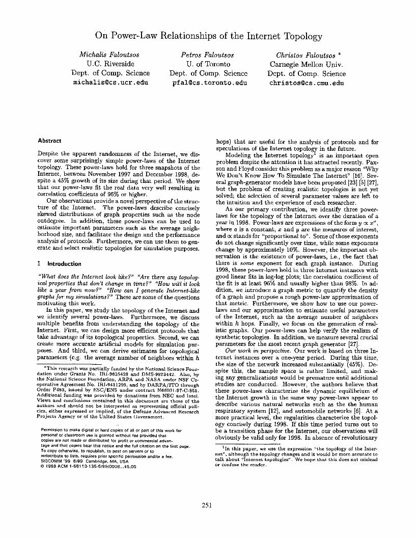
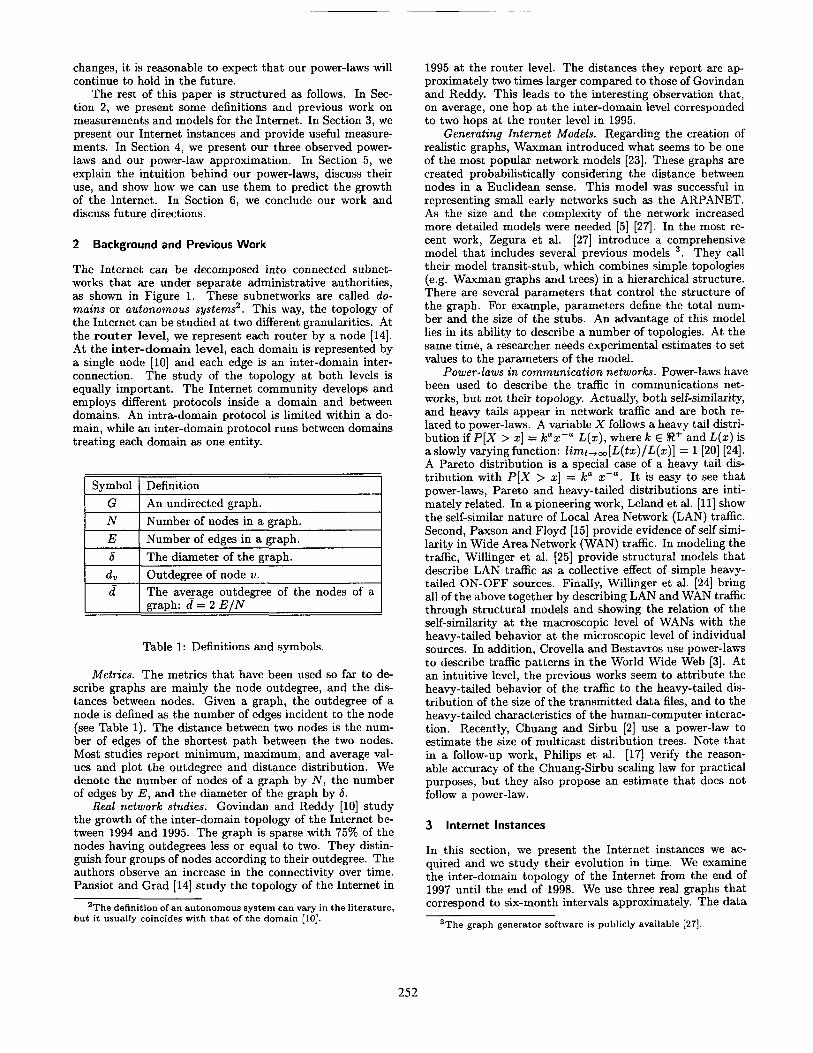
In this section, we study the outdegrees of the nodes. We sort the nodes in decreasing order of outdegree, d,, and plot the (rU, d,) pairs in log-log scale. The results are shown in Figures 3 and 4. The measured data is represented by diamonds, while the solid line represents the Ieaat-squares approximation.

A striking observation is that the plots are approximated well by the linear regression. The correlation coefficient is higher than 0.974 for the inter-domain graphs and 0.948 for the Rout-95 graph. This leads us to the following power-law and definition.

Power-Law 1 (rank exponent) The outdegree, d,, of a node v, is proportional to the rank of the node, rv, to the power of a constant, R:

d,, K r?

Definition 1 Let us sort the nodes of a graph in decreasing order of outdegree. We define the rank exponent, R, to be

the slope of the plot of the outdegrees of the nodes versus the rank of the nodes in log-log scale.

For the three inter-domain instances, the rank exponent, R, is -0.81, -0.82 and -0.74 in chronological order as we see in Appendix B. The rank exponent of the Rout-95 graph, -0.48, is different compared to that of the first three graphs. This is something that we expected, given the differences in the nature of the graphs. On the other hand, this difference suggests that the rank exponent can distinguish graphs of different nature, although they both follow Power-Law 1. This property can make the rank exponent a powerful metric for characterizing families of graphs, see Section 5.

Intuitively, Power-Law 1 most likely reflects a principle of the way domains connect; the linear property observed in our four graph instances is unlikely to be a coincidence. The power-law seems to capture the equilibrium of the trade- off between the gain and the cost of adding an edge from a financial and functional point of view, as we discuss in Section 5.

Extended Discussion - Applications. We can estimate the proportionality constant for Power-Law 1, if we require that the minimum outdegree of the graph is one (dN = 1). This way, we can refine the power-law as follows.

Lemma 1 The outdegree, d,, of a node v, is a function of the rank of the node, rV and the rank exponent, I?., as follows

1 d, = ~a rc

Proof. The proof can be found in Appendix C. Finally, using lemma 1, we relate the number of edges

with the number of nodes and the rank exponent.

Lemma 2 The number of edges, E, of a graph can be estimated as a function of the number of nodes, N, and the rank exponent, R, as follows:

EC ’ 2(7Z+1) (1 -

Proof. The proof can be found in Appendix C. Note that Lemma 2 can give us the number of edges as

a function of the number of nodes for a given rank exponent. We tried the lemma in our datasets and the estimated number of edges differed by 9% to 20% from the actual number of edges. More specifically for the Int-12-98, the lemma underestimates the number of edges by 10%. We can get a closer estimate (3.6%) by using a simple linear interpola- tion in the number of edges given the number of nodes. Note that the two prediction mechanisms are different: our lemma does not need previous network instances, but it needs to know the rank exponent. However, given previous network instances, we seem to be better off using the linear inter- polation according to the above analysis. We examined the sensitivity of our lemma with respect to the value of rank exponent. A 5% increase (decrease) in the absolute value of the rank exponent increases (decreases) the number of edges by 10% for the number of nodes in Int-12-98.

4.2 The outdegree exponent 0

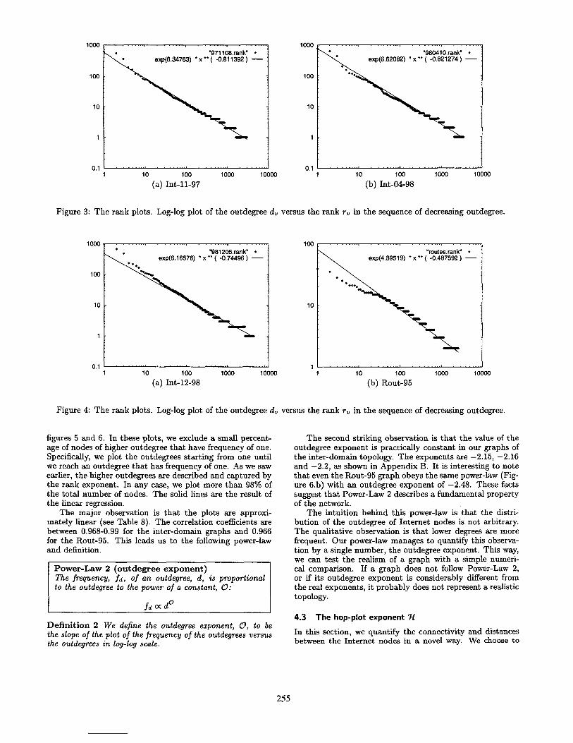
In this section, we study the distribution of the outdegree of the graphs, and we manage to describe it concisely by a single number. Recall that the frequency, fd, of an outdegree, d, is the number of nodes with outdegree d. We plot the frequency fd versus the outdegree d in log-log scale in

254

"971108.rank exp(6.34763) l x "( -0.611392 )

"960410.rank" l

exp(6.62082) 'x*'( -0.821274 ) -

10 100 1000 10000 1 10 100 1000 10000

(a) Int-11-97 (b) Int-04-98

Figure 3: The rank plots. Log-log plot of the outdegree d, versus the rank ru in the sequence of decreasing outdegree.

. . '961205.rank" l : exp(6.16576) 'x"( -0.74496) - :

10

1 10 100 1000 1ooOe 1 10 100 loo0 10000

(a) Int-12-98 (b) Rout-95

Figure 4: The rank plots. Log-log plot of the outdegree d, versus the rank r,, in the sequence of decreasing outdegree.

figures 5 and 6. In these plots, we exclude a small percent- The second striking observation is that the value of the age of nodes of higher outdegree that have frequency of one. outdegree exponent is practically constant in our graphs of Specifically, we plot the outdegrees starting from one until the inter-domain topology. The exponents are -2.15, -2.16 we reach an outdegree that has frequency of one. As we saw and -2.2, as shown in Appendix B. It is interesting to note earlier, the higher outdegrees are described and captured by that even the Rout-95 graph obeys the same power-law (Fig- the rank exponent. In any case, we plot more than 98% of ure 6.b) with an outdegree exponent of -2.48. These facts the total number of nodes. The solid lines are the result of suggest that Power-Law 2 describes a fundamenbal property the linear regression. of the network.

The major observation is that the plots are approximately linear (see Table 8). The correlation coefficients are between 0.968-0.99 for the inter-domain graphs and 0.966 for the Rout-95. This leads us to the following power-law and definition.

Power-Law 2 (outdegree exponent) The frequency, fd, of an outdegree, d, is proportional to the outdegree to the power of a constant, C?

The intuition behind this power-law is .that the distribution of the outdegree of Internet nodes is not arbitrary. The qualitative observation is that lower degrees are more frequent. Our power-law manages to quantify this observation by a single number, the outdegree exponent. This way, we can test the realism of a graph with a simple numerical comparison. If a graph does not follow Power-Law 2, or if its outdegree exponent is considerably different from the real exponents, it probably does not represent a realistic topology.

Definition 2 We define the outdegree exponent, 0, to be the slope of the plot of the frequency of the outdegrees versus the outdegrees in log-log scale.

4.3 The hop-plot exponent Yl

In this section, we quantify the connectivity and distances between the Internet nodes in a novel way. We choose to

255

‘971108.0ut’ l

~~(7.68565) * x l * ( -2.16632 ) - ‘980410.0Ut” l

exp(7.69793) * x ** ( -2.16356) -

100 100

10 10

.

1 1 1

(a) Id-:10-W

100 1

(b) Int-ii-98 100

Figure 5: The outdegree plots: Log-log plot of frequency fd versus the outdegree d.

“981205.0ur l

exp(8.11393) l x ** ( -2.20266 ) - -r0utes.out~ l

exp(8.52124) * x”( -2.48628) - :

(a) Int-1198 loo

(b) Rou:95 loo

Figure 6: The outdegree plots: Log-log plot of frequency fd versus the outdegree d.

study the size of the neighborhood within some distance, instead of the distance itself. Namely, we use the total number of pairs of nodes P(h) within h hops, which we define as the total number of pairs of nodes within less or equal to h hops, including self-pairs, and counting all other pairs twice.

Let us see the intuition behind the number of pairs of nodes P(h). For h = 0, we only have the self-pairs: P(0) = N. For the diameter of the graph 6, h = 6, we have the self- pairs plus all the other possible pairs: P(b) = N*, which is the maximum possible number of pairs. For a hypothetical ring topology, we have P(h) oc h’, and, for a 2-dimensional grid, we have P(h) 0: h*, for h < b. We examine whether the number of pairs P(h) for the Internet follows a similar power-law.

In figures 7 and 8, we plot the number of pairs P(h) as a function of the number of hops h in log-log scale. The data is represented by diamonds, and the dotted horizontal line represents the maximum number of pairs, which is iV*. We want to describe the plot by a line in least-squares fit, for h < 6, shown as a solid line in the plots. We approximate the first 4 hops in the inter-domain graphs, and the first 12 hops in the Rout-95. The correlation coefficients are is 0.98

for inter-domain graphs and 0.96, for the Rout-95, as we see in Appendix B. Unfortunately, four points is a rather small number to verify or disprove a linearity hypothesis ex- perimentally. However, even this rough approximation has several useful applications as we show later in this section.

Approximation 1 (hop-plot exponent) The total number of pairs of nodes, P(h), within h hops, is proportional to the number of hops to the power of

Definition 3 Let us plot the number of pairs of nodes, P(h), within h hops uersus the number of hops in log-log scale. For h < 6, we define the slope of this plot to be the hop-plot exponent,%.

Observe that the three inter-domain datasets have practically equal hop-plot exponents; 4.6,4.7, and 4.86 in chronological order, as we see in Appendix B. This shows that the hop-plot exponent describes an aspect of the connectivity of the graph in a single number. The Rout-95 plot, in fig. 8.b,

256

1e+11 \

1e+lO -

le+09 r

le+OB

le+07 -

le+O6 r

“971108.hopplot” l

exp(9.84805) * x l * ( 4.62706 ) - : maximum number of pairs ........

1e+11 t

le+lO -

1e+o9 I

le+O6 7

le+07 -

le+O6 -

“980410.hopplot” l

exp(10.0876) * x** ( 4.71768) - : maximum number of pairs ........

10000 -

1000 1 10 1 10

(a) Int-11-97 (b) Int-04-98

Figure 7: The hop-plots: Log-log plots of the number of pairs of nodes P(h) within h hops versus the number of hops h.

;., [:I maxlmum number of paws ........

;.f i/ maxlmum number of pairs ....-...

,E--::;‘.......................... ; l=J$-/+ I

‘:I: 1 10

(a) Int-12-98

1000 t 1

(b) Rou::95

J 100

Figure 8: The hop-plots: Log-log plots of the number of pairs of nodes P(h) within h hops versus the number of hops h.

ham more points, and thus, we can argue for its linearity with more confidence. The hop-plot exponent of Rout-95 is 2.8, which is much different compared to those of the inter-domain graphs. This is expected, since the Rout-95 is a sparser graph. Recall that for a ring topology, we have 3t = 1, and, for a 2-dimensional grid, we have ‘H = 2. The above observations suggest that the hop-plot exponent can distinguish families of graphs efficiently, and thus, it is a good metric for characterizing the topology.

Extended Discussion - Applications. We can refine Approximation 1 by calculating its proportionality constant. Let us recall the definition of the number of pairs, P(h). For h = 1, we consider each edge twice and we have the self-pairs, therefore: P(1) = N + 2 E. We demand that Approximation 1 satisfies the previous equation as an initial condition.

Lemma 3 The number of pairs within h hops is

h < 6 h>b

where c = N + 2 E to satisfy initial conditions.

In networks, we often need to reach a target without knowing its exact position [7] [l]. In these cases, selecting the extent of our broadcast or search is an issue. On the one hand, a small broadcast will not reach our target. On the other hand, an extended broadcast creates too many messages and takes a long time to complete. Ideally, we want to know how many hops are required to reach a “sufficiently large” part of the network. In our hop-plots, a promising solution is the intersection of the two asymptote lines: the horizontal one at level N2 and the asymptote with slope ?Y. We calculate the intersection point using Lemma 3, and we define:

Definition 4 (effective diameter) Given a graph with iV nodes, E edges, and 7-l hop-plot exponent, we define the effective diameter, 6,f, as:

N2 l&f= -

( >

l/N

N+2E

Intuitively, the effective diameter can be understood as follows: any two nodes are within 6,s hops from each other with high probability. We verified the above statement ex- perimentally. The effective diameters of our inter-domain

257

4500 I Actual -

4000 - using hopplot -+-. -. using avg OutdeQree a../

3500 -

3wo -

2500 -

2000 -

1500 -

1000 -

500 t /(I/----------- ,____-_ -- __._._______ ____.. -........‘..

______:

1 1.5 2 2.5 3 3.5 4 Number of Hops

Figure 9: Average neighborhood size versus number of hops the actual, and estimated size a) using hop-plot exponent, b) using the average outdegree for Int-12-98.

Hops hop-plot avg. outdegree

1 0.02 1.82

I 2 I -0.66 I -0.93 I

I 3 I -0.47 I -0.95 I I 4 I 0.17 I -0.93 I

Table 3: The relative error of the two estimates for the average neighborhood size with respect to the real value. Negative error means under-estimate.

graphs was slightly over four. Rounding the effective diameter to four, approximately 80% of the pairs of nodes are within this distance. The ceiling of the effective diameter is five, which covers more than 95% of the pairs of nodes.

An advantage of the effective diameter is that it can be calculated easily, when we know N, and ‘U. Recall that we can calculate the number of edges from Lemma 2. Given that the hop-plot exponent is practically constant, we can estimate the effective diameter of future Internet instances as we do in Section 5.

Furthermore, we can estimate the average size of the neighborhood, NN(h), within h hops using the number of pairs P(h). Recall that P(h) - N is the number of pairs without the self-pairs.

NN(h) = 7 - 1

Using Equation 1 and Lemma 3, we can estimate the average neighborhood size.

Lemma 4 The average size of the neighborhood, NIV(h), within h hops as a function of the hop-plot exponent, ‘fl, for h << 6, is

NIV(h) = + hS - 1

where c = N + 2 E to satisfy initial conditions.

The average neighborhood is a commonly used parameter in the performance of network protocols. Our estimate is an improvement over the commonly used estimate that

uses the average outdegree [26] [7] which we call average- outdegree estimate:

NN’(h) = d (6- l)h-l

In figure 9, we plot the actual and both estimates of the average neighborhood size versus the number of hops for the Int-12-98 graph. In Table 3, we show the normalized error of each estimate: we calculate the quantity: (p - r)/r where p the prediction and T the real value. The results for the other inter-domain graphs are similar. The superiority of the hop-plot exponent estimate is apparent compared to the average-outdegree estimate. The discrepancy of the average- outdegree estimate can be explained if we consider that the estimate does not comply with the real data; it implicitly assumes that the outdegree distribution is uniform. In more detail, it assumes that each node in the periphery of the neighborhood adds d - 1 new nodes at the next hop. Our data shows that the outdegree distribution is highly skewed, which explains why the use of the hop-plot estimate gives a better approximation.

The most interesting difference between the two estimates is qualitative. The previous estimate considers the neighborhood size exponential in the number of hops. Our estimate considers the neighborhood as an ‘?-l-dimensional sphere with radius equal to the number of hops, which is a novel way to look at the topology of a network5. Our data suggests that the hop-plot exponent-based estimate gives a closer approximation compared to the average-outdegree- based metric.

4.4 The eigen exponent &

In this section, we identify properties of the eigenvalues of our Internet graphs. There is a rich literature that proves that the eigenvalues of a graph are closely related to many basic topological properties such as the diameter, the number of edges, the number of spanning trees, the number of connected components, and the number of walks of a certain length between vertices, as we can see in [8] and [4]. All of the above suggest that the eigenvalues intimately relate to topological properties of graphs.

We plot the eigenvalue Xi versus i in log-log scale for the first 20 eigenvalues. Recall that i is the order of X; in the decreasing sequence of eigenvalues. The results are shown in Figure 10 and Figure 11. The eigenvalues are shown as diamonds in the figures, and the solid lines are approximations using a least-squares fit.

Observe that in all graphs, the plots are practically linear with a correlation coefficient of 0.99, as we see in Ap- pendix B. It is rather unlikely that such a canonical form of the eigenvalues is purely coincidental, and we therefore conjecture that it constitutes an empirical power-law of the Internet topology.

Power-Law 3 (eigen exponent) TILe eigenvalues, A;, of a graph are proportional to the order, i, to the power of a constant, E:

Xi o( i’

Definition 5 We define the eigen exponent, E, to be the slope of the plot of the sorted eigenvalues versus their order in log-log scale.

5Note that our results focus on relatively small neighborhoods compared to the diameter h <( 6. Other experimental studies focus on neighborhoods of larger radius [17].

258

ber of nodes, the number of edges, and the average neighborhood size.

l We propose power-law exponents, instead of averages, as an efficient way to describe the highly-skewed graph metrics which we examined.

.4part from their theoretical interest, we showed a number of practical applications of our power-laws. First, our power-laws can assess the realism of synthetic graphs, and enhance the validity of our simulations. Second, they can help analyze the average-case behavior of network protocols. For example, we can estimate the message complexity of protocols using our estimate for the neighborhood size. Third, the power-laws can help answer “what-if” scenar- ios like “what will be the diameter of the Internet, when the number of nodes doubles?” ‘( what will be the number of edges then?”

In addition, we decompose and measure the Internet in a way that relates to the state-of-the-art graph generation models. This decomposition provides measurements that facilitate the selection of parameters for the graph generators.

For the future, we believe that our suggestion to look for power-laws will open the floodgates to discovering many additional power-laws of the Internet topology. Our opti- mism is based on two facts: (a) power-laws are intimately related to fractals, chaos and self-similarity [21] and (b) there is overwhelming evidence that self-similarity appears in a large number of settings, ranging from traffic patterns in networks [24], to biological and economical systems [12].

ACKNOWLEDGMENTS. We would like to thank Mark Craven, Daniel Zappala, and Adrian Perrig for their help in earlier phases of this work. The authors are grateful to Pansiot and Grad for providing the Rout-95 routers data. We would also like to thank Vern Paxson, and Ellen Zegura for the thorough review and valuable feedback. Finally, we would like to thank our mother Sofia Faloutsou-Kalamara and dedicate this work to her.

References

PI

PI

[31

[41

[51

[61

171

PI

PI

K. Carlberg and J. Crowcroft. Building shared trees using a one-to-many joining mechanism. ACM Computer Commu- nication Review, pages 5-11, January 1997.

J. Chuang and M. Sirbu. Pricing multicast communications: A cost based approach. In Proc. of the INET’98, 1998.

M. Crovella and A. Bestavros. Self-similarity in World Wide Web traffic, evidence and possible causes. SIGMETRICS. pages 160-i69, 1996. -

D. M. Cvetkovit, M. Boob, and H. Sachs. Spectra of Graphs. Academic press, 1979.

M. Doar. A better model for generating test networks. Proc. Global Internet, IEEE, Nov. 1996.

Christos Faloutsos and Ibrahim Kamel. Beyond uniformity and independence: Analysis of R-trees using the concept of fractai dimension. In- Proc. ACM SIGACT-SIGMOD- SIGART PODS, oages 4-13. Minneanolis. MN. Mav 24-26 1994. Also availidle-% CS-Tk-3198, GMIkCS-i’R-93-130.

M. Faloutsos, A. Banerjea, and R. Pankaj. QoSMIC: a &OS Multicast Internet protocol. ACM SIGCOMM. Computer Communication Review., Sep 2-4, Vancouver BC 1998.

M. Faloutsos, P. Faloutsos, and C. Faloutsos. Power-laws of the Internet topology. Technical Report UCR-CS-99-01, University of California Riverside, Computer Science, 1999.

National Laboratory for Applied Network Research. Routing data. Supported by NSF, http://moat.nlanr.net/Routing/rawdata/, 1998.

[101

1121

[I31

[I41

P51

WI

[I71

PI

P-4

PO1

PI

[‘=I

[231

P41

1251

[261

P71

PI

R. Govindan and A. Reddy. An analysis of internet inter- domain topology and route stability. Proc. IEEE INFO- COM, Kobe, Japan, April 7-11 1997.

W.E. Leland, M.S. Taqqu, W. Willinger, and D.V. Wilson. On the self-similar nature of ethernet traffic. IEEE Trans- actions on Networking, 2(1):1-15, February 1994. (earlier version in SIGCOMM ‘93, pp 183-193).

B. Mandelbrot. I+actal Geometry of Nature. W.H. Freeman, New York, 1977.

J. Moy. Multicast routing extensions for OSPF. ACM Con- nunications, 37(8):61-66, 1994.

J.-J. Pansiot and D Grad. On routes and multicast trees in the Internet. ACM Computer Communication Review, 28(1):41-50, January 1998.

V. Paxson and S. Floyd. Wide-area traffic: The failure of Poisson modeling. IEEE/ACM Transactions on Networking, 3(3):226-244, June 1995. (earlier version in SIGCOMM’SI, pp. 257-268).

V. Paxson and S. Floyd. Why we don’t know how to simulate the internet. Proceedings of the 1997 Winter Simulation Conference, December 1997.

G. Philips, S. Shenker, and H. Tangmunarunkit. Scaling of multicast trees: Comments on the chuang-sirbu scaling law. ACM SIGCOMM. Computer Communication Review., Sep 1999.

William H. Press, Saul A. Teukolsky, William T. Vetterling, and Brian P. Flannery. Numerical Recipes in C. Cambridge University Press, 2nd edition, 1992.

Y. Rekhter and T. Li (Eds). A Border Gateway Protocol 4 (BGP-4). Internet-Draft.:draft-ietf-idr-bgp4-08.txt available from ftp://ftp.ietf.org/internet-drafts/, 1998.

S. R. Resnick. Heavy tail modeling and teletraffic data. An- nals of Statistics, 25(5):1805-1869, 1997.

Manfred Schroeder. l+actals, Chaos, Power Laws: Minutes from an Infinite Paradise. W.H. Freeman and Company, New York, 1991.

D. Waitzman, C. Partridge, and S. Deering. Distance vector multicast routing protocol. IETF RFC 1075, 1998.

B. M. Waxman. Routing of multipoint connections. IEEE Journal of Selected Areas in Communications, pages 1617- 1622, 1988.

W. Willinger, V. Paxson, and M.S. Taqqu. Self-similarity and heavy tails: Structural modeling of network traffic. In A Practical Guide to Heavy Tails: Statistical Techniques and Applications, 1998. Adler, R., Feldman, R., and Taqqu, M.S., editors, Birkhauser.

Walter Willinger, Murad Taqqu, Robert Sherman, and Daniel V. Wilson. Self-similarity through high variability: statistical analysis of ethernet LAX traffic at the source level. ACM SIGCOMM’95. Computer Communication Re- view, 25:100-113, 1995.

D. Zappala, D. Estrin, and S. Shenker. Alternate path routing and pinning for interdomain multicast routing. Technical Report USC CS TR 97-655, U. of South California, 1997.

E. W. Zegura, K. L. Calvert, and M. J. Donahoo. A quanti- tative comparison of graph-based models for internetworks. IEEE/ACM Transactions on Networking, 5(6):770-783, De- cember 1997. http://www.cc.gatech.edu/projects/gtitm/.

G.K. Zipf. Humun Behauior and Principle of Least Eflort: An Introduction to Human Ecology. Addison Wesley, Cam- bridge, Massachusetts, 1949.

261

Int-11-97 Int-04-98 Int-12-98

nodes 3015 3530 4389

edges 5156 6432 8256

avg. 3.42 3.65 3.76 outdegree

max. 590 745 979 outdegree

diameter 9 11 10

avg. distance 3.76 3.77 3.75

Table 6: The evolution of the Internet at the inter-domain level.

Int-11-97 Int-04-98 Int-12-98

#nodes in 50.05 45.05 40.76 trees (%)

#trees over 10.12 10.26 9.4 #nodes (%)

max depth 3 3 3

avg. tree size 4.9 4.4 4.3

core 4.7 4.9 4.9 outdegree

Table 7: The evolution of the Internet considering the core and the trees.

A Decomposing the Internet

We analyze the Internet in a way that suits the graph generator models [27]. The measurements we present can facilitate the selection of parameters for these generators.

We study the graphs through their decomposition into two components: the tree component that contains all nodes that belong exclusively to trees and the core component that contains the rest of the nodes including the roots of the trees. We measure several parameters from this decomposition that are shown in Table 7. These results leads to the following observations.

Approximately half of the nodes are in trees 40-50%

The number of nodes in trees decreased with time by 10% means that the Internet becomes more connected all around.

The maximum tree depth is 3, however more than 80% of the trees have depth one.

More than 95% of the tree-nodes have a degree of one. This leads to the following interesting observation: if we remoue the nodes with outdegree one from the orig- inal graph, we practically get the core component.

These observations can help users select appropriate values for the parameters used in various graph generation techniques [27].

1 Exponent 1 Int-11-97 1 Int-04-98 1 Int-12-98 11 Rout-95 1

rank -0.81 -0.82 -0.74 -0.48 ACC 0.981 0.979 0.974 0.948

outdeeree ACC um

-2.15 0.991

-2.16 -2.20 I -2.48 0.979 0.96s 0.966

hop-plot 4.62 4.71 4.86 2.83 ACC 0.983 0.981 0.980 0.991

eigen -0.471 -0.502 -0.487 -0.17 ACC 0.990 0.989 0.991 0.994

Table 8: An overview of all the exponents for all our graphs. Note that ACC is the absolute value of the correlation coefficient .

C The Proofs

Here we prove the Lemmas we present in our paper. Lemma 1. The outdegree, d,, of a node v, is a function

of the rank of the node, rV and the rank exponent, R, as follows

d, = & rr Proof. We can estimate the proportionality constant,C, for Power-Law 1, if we require that the outdegree of the N-th node is one, dN = 1.

dN = CN R *

C = l/N” (2)

We combine Power-Law 2 with Equation 2, and conclude the proof. n

Lemma 2. The number of edges, E, of a graph can be estimated as a function of the number of nodes, N, and the rank exponent, R, as follows:

E= 1

2 (R+l) (1 - j&i) N

Proof: The sum of all the outdegrees for all the ranks is equal to two times the number of edges, since we count each edge twice.

2E = ed,

In the last step, above we approximate the summation with an integral. Calculating the integral concludes the proof. n

B The Exponents of Our Power-Laws

We present the exponents of our power-laws in Table 8.

on power-law relationships of the internet...

Documents