on migrant selectivity eric r. jensen college of william ...economics.wm.edu/wp/cwm_wp32.pdf · on...

On Migrant Selectivity

Eric R. Jensen College of William and Mary

Sarah M. Gale Accenture

Paul E. Charpentier University of Wisconsin-Madison

College of William and Mary Department of Economics Working Paper Number 32

July 2006

We thank Yana Rodgers, George Grayson, David Card and David Jaeger for helpful comments and Dheeraj Jagadev for research assistance.

COLLEGE OF WILLIAM AND MARY DEPARTMENT OF ECONOMICS WORKING PAPER # 32 July 2006


Abstract

Recent migrants to the United States have displayed lower earnings levels and a slower rate of earnings convergence with natives than previous immigrants. Borjas has argued that this reflects negative selectivity of immigrants; others, including Card, Chiquiar and Hanson, and Duleep and Regets, question this contention. Some of the ambiguity is due to measurement problems, with educational attainment (or its labor market consequences) used in place of unobserved migrant quality. We suggest that constraints in the supply of education in sending regions significantly limit the usefulness of educational attainment or related measures as proxies for migrant quality. We propose an alternative measure of migrant quality that incorporates education supply constraints, and present evidence of Mexican migrants self-selecting positively on ability. JEL Codes: J24, J61 Keywords: Migration, self-selection, human capital Eric R. Jensen (corresponding author) Sarah M. Gale Thomas Jefferson Program in Public Policy and Accenture Department of Economics 11951 Freedom Drive College of William and Mary Reston, Virginia 20190 P.O. Box 8795 [email protected] Williamsburg, VA 23187-8795 [email protected] Paul E. Charpentier Department of Economics University of Wisconsin-Madison 1180 Observatory Drive Madison, WI 53706-1393 [email protected]

1


In an elegant and important theoretical paper, Roy (1951) develops a model of

endogenous selection into the occupations of “hunter” and “fisher.” In this model,

relative ability at hunting or fishing and subsequent expected income from whichever

occupation is chosen are directly tied. An important implication of Roy’s model is that

with comparable mean earnings in each occupation, those with low ability will avoid the

occupation where the income distribution has a longer left-hand tail, because they are

likely to be farther below mean earnings than had they chosen the distribution less

penalizing to low ability. Conversely, those with high ability will prefer the occupation

with the more diffuse distribution of income, as this allows a greater reward for ability.

In an influential body of work, Borjas (1990, 1991, 1994, 1999) has extended this

model to analyses of migration, where the choice actors make is country of residence

(effectively a basket of occupations and earnings), and the model is applied to

international migration to the United States. Borjas’ assumption, after Roy, is that

placement within an income distribution is reflective variously of ability, skills or “ethnic

capital.” Borjas (1994) defines ethnic capital conceptually as the quality of the ethnic

environment in which a person is raised and operationally as the average educational

attainment in a sending country. He posits that this ethnic capital influences the skills

and labor market outcomes of the children of immigrants, and suggests that the difference

in US earnings between immigrants and natives is useful as a proxy for relative skill

differentials. In this setting, even if mean incomes in both countries were the same, those

in the left tail of the relatively diffuse Mexican income, ability, or skills distribution

would have an incentive to migrate to the relatively egalitarian United States.

2

In later work of Borjas and in work of other contributors to this literature,

discussion centers on the placement of migrants within the distribution of skills, with

special regard for the transferability of skills acquired in the sending country. This

discussion is couched in human capital terms. Duleep and Regets (1999), for example,

predict that migrants with more to gain in investing in human capital will do so. This is

partly driven by low opportunity cost and partly by high expected benefits. Their

empirical prediction is that earnings will grow faster for immigrants than for the native

born. Schoeni (1997) finds less reassuring evidence on this count. Chiquiar and Hanson

(2005) compare counterfactual predictions of skill premia for US immigrants, had they

remained in the Mexican labor market, with the actual distribution of US earnings. In

contrast to Borjas, they find that Mexican immigrants would fall in the middle and upper

portion of the Mexican wage distribution.

As Borjas points out, at issue is not just the pace of earnings growth, but the

difference in initial earnings levels between immigrants and native-born populations.

Following a narrow interpretation of Roy, the issue is the labor market skills of migrants.

Assuming that training is provided efficiently in sending countries, the least able are also

the least trained. They have chosen to accumulate little human capital because the net

benefit to them is low. Borjas’ policy recommendation to limit immigration (e.g., Borjas

1999) follows unavoidably.

Roy’s is very much a story of functioning markets, but in many developing

countries, educational resources are heavily concentrated in urban areas. The populations

in these countries typically are substantially rural. Because educational supply

constraints are more likely to bind in rural areas, all else constant, levels of educational

3

attainment in rural areas will be lower. If this is the case, interpreting educational

differences across the population of migrants from developing countries as reflective of

broader quality differentials clearly is problematic, since some high-ability individuals

from educationally supply-constrained rural areas may have low levels of educational

attainment. The Borjas recommendation to limit low-skill immigrants carries less force

in this case, as there may be substantial gains to the host society accruing from training

those migrants who, due to supply constraints in sending countries, have low levels of

human capital upon arrival but, because of their high ability levels, have relatively high

expected gains from human capital accumulation.

We use data from the Mexican Migration Project to construct a model that

accounts for potentially supply-constrained access to education within Mexico. We find

that it is relatively better-educated individuals from impoverished, education-constrained

regions of Mexico, rather than a broad cross-section of the less educated, who are most

likely to migrate to the United States. The efficiency of exclusionary immigration

policies based on the presumption of low migrant ability therefore appear to be of

questionable efficiency vis-à-vis training or other more migrant-friendly policies that

would allow the host country to capitalize on highly able but suboptimally trained

migrants.

Negative or positive selection of immigrants?

The Borjas model is one of negative selection, where those with the lowest

ability, and so lowest potential earnings in either Mexico or the US, are most likely to

migrate to the US. For example, Borjas (1994, p. 1677) states that

4

Relative to natives, immigrants were about 21.7 percent more likely to be

high school dropouts in 1970, but are now more than twice as likely to be

high school dropouts.

Borjas interprets this apparent decline in immigrant quality as being attributable to

changes in the national origin mix of the immigrant flow, as migrant flows have

increasingly consisted of individuals from low-income countries, and offers this sort of

analysis as evidence of negative selection of migrants to the United States.

It has proven difficult to isolate migrant ability empirically. Borjas has regressed

a dummy variable representing the degree of income inequality in the sending country

relative to the United States or, closely related, the ratio of earnings of the top households

to the earnings of lowest-income households in the sending country, on the level and rate

of change of immigrant’s earnings (Borjas 1990). He finds that either regressor is

inversely associated with earnings. Borjas takes this as reflective of adverse selection of

migrants on ability or skill differentials, but the finding that countries with unequal

income distributions are likely to send migrants to the United States is at best an inexact

test of the Roy model. We will return to an alternative explanation of Borjas’ findings

later in the paper.

Chiswick (1999) notes that the Roy model is a special case of the human capital

model of migration. According to Chiswick, negative selection, if it exists, is a

tempering influence on what is likely, according to typical human capital models of

migration (e.g., Sjaastad 1962) to be positive selection overall. Chiquiar and Hanson

(2005) point out that illegal border crossing entails lower costs for the more educated

(who have less difficulty obtaining the needed cash), and that these costs are important in

the selection process. In this view, differences in mean earnings between countries

5

swamp the differences in earnings variance that drive the Roy model. High ability

individuals, able to bear the financial cost of migration from low-income countries yet

still benefiting from higher wages in the United States, are drawn there. Chiquiar and

Hanson project as counterfactuals the Mexican earnings of US immigrants, and find them

to be solidly in the middle of the Mexican earnings distribution.

The difficulty with such contentions lies in reconciling them with findings like

Borjas’ on immigrant quality. If migrants actually are those of high earning capacity,

relative to their peers at home, what accounts for the finding that, at least for some

immigrant groups, immigrant earnings are lower and grow more slowly compared to

natives? Schoeni (1997) brings this finding vividly home, showing that Mexican and

Central American emigrants have low initial levels and low rates of growth of earnings

compared to US natives, and low rates of growth compared to those who came to the US

from other countries. Schoeni controls for migrant education, and notes that Mexicans

educated in the United States had nearly twice the schooling of those educated in Mexico,

and a much smaller earnings differential compared to the native born. Card (2005) also

points out that earnings of foreign-born workers are much lower than those of the native-

born, and, attributing this to poor training and language skills of immigrants, sees little

prospect of the gap closing. However, using the 1995-2002 Current Population Survey,

Card shows that the children of immigrants have more education and higher wages than

comparable third-and-higher generation native born. Taken together, the findings of

Schoeni and Card are consistent with the view that some migrants possess innate abilities,

attitudes, or other potentially heritable qualities at least equal to non-migrants from their

6

countries of origin, but that their training is sufficiently poor relative to the native-born to

sustain a substantial earnings gap.

Stark and Taylor have argued in a series of papers for the importance of

household-level rather than individual-level decision making in migration. In this

context, they develop a model of relative household deprivation, and test it on a small

sample of Mexican households in two rural villages (Stark and Taylor 1991). They

estimate a multinomial logit model of the log odds of migrating domestically or

internationally, versus not migrating at all. While they base their discussion on raw

coefficients and do not present marginal effects, these are straightforward to calculate.

From their results, we calculate a marginal effect of income on the probability of

international migration of 0.41, and a marginal effect of relative income deprivation, a

measure that apparently is measured in the same units as income, of 0.09. Thus, income-

increasing policy changes may have differing effects on rural emigration, according to

the extent that effects of such changes meet different reactions across the income

distribution. Our calculated marginal effect of a year of educational attainment on the

probability of US migration, based on the Stark and Taylor multinomial logit coefficients,

is -0.02.

We are unable to attach statistical significance levels to any of the Stark and

Taylor marginal effects, but they are suggestive of two things. First, relative economic

standing matters. It appears that in this case, for all but the most inegalitarian policies,

effects on US migration driven by relative income standing are likely to be dominated by

absolute income levels but that nevertheless, the marginal effect of relative deprivation is

roughly 22% as large as the marginal effect of absolute income levels. Secondly, it

7

appears from the Stark and Taylor results that the less educated, measured in absolute

rather than relative terms, are more likely to migrate from rural Mexico to the US. It

would have been appealing in the present context had Stark and Taylor examined the

impact of relative education, as a proxy for relative deprivation based on future earnings.

Unfortunately, given the highly geographically concentrated sample they employ, there is

little supply-side variability in education Stark and Taylor could have exploited in these

data, and so little that could have been said in any case about relative education and

migration.

A model of Mexican-US migration

There are three characteristics that drive our model, none controversial:

1. Migrants choose to migrate where the wage differential, net of migration

costs, is positive.

2. Human capital accretions increase wages in both sending and receiving

labor markets, though at varying rates.

3. Human capital levels depend on an initial endowment and on subsequent

accumulation, and such accumulation is costly.

We assume that the wage received by an individual in Mexico, w0, is a function of

the base Mexican wage µ0, human capital accumulation h, and the return to human

capital in Mexico, !0(h), where !0">0.5 Human capital accumulation is a function of

ability a and skill accumulation s, with skills contributing to human capital accumulation

at constant rate #0 in Mexico. Skills are less costly for those with high ability or for those

5 We suppress an individual-specific subscript throughout for the sake of simplicity.

8

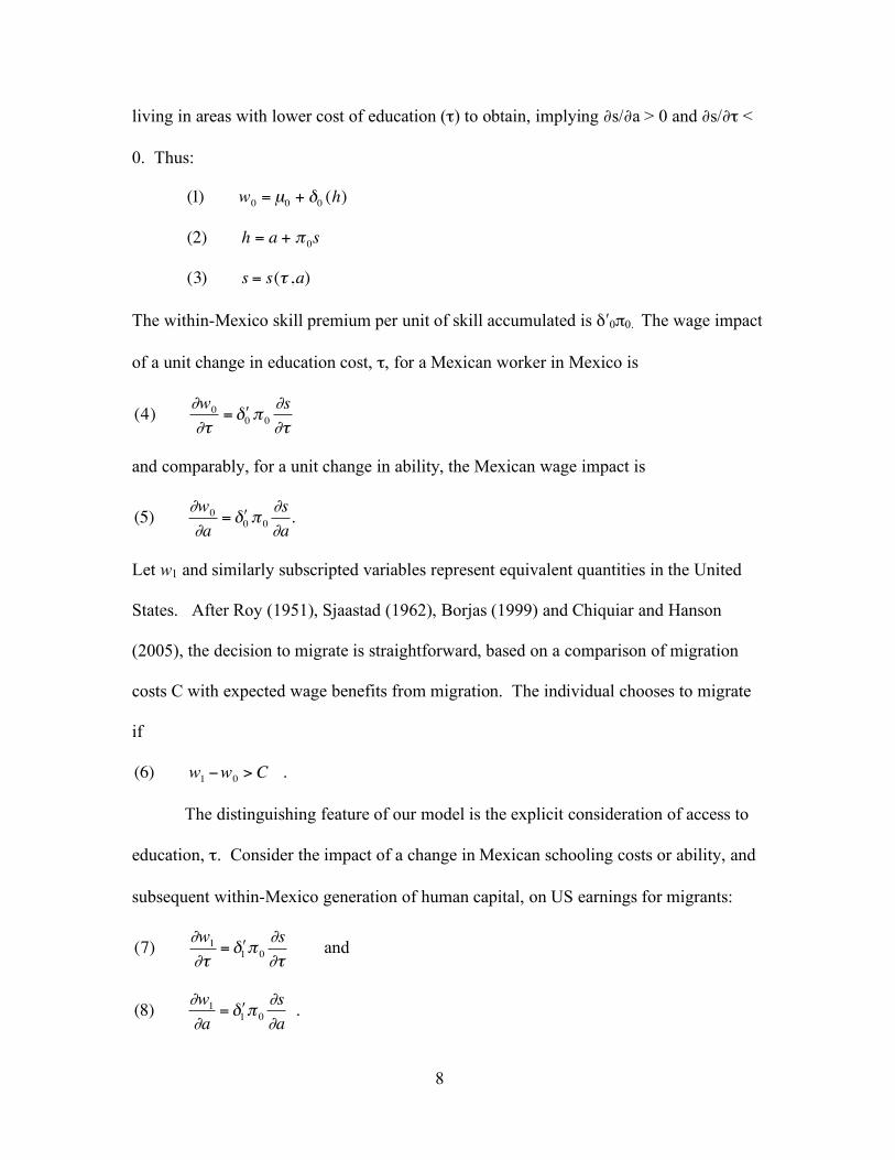
living in areas with lower cost of education ($) to obtain, implying %s/%a > 0 and %s/%$ <

0. Thus:

!

(1) w0

= µ0

+ "0(h)

!

(2) h = a + "0s

!

(3) s = s(" ,a)

The within-Mexico skill premium per unit of skill accumulated is !"0#0. The wage impact

of a unit change in education cost, $, for a Mexican worker in Mexico is

!

(4)"w

0

"#= $ %

0&0

"s

"#

and comparably, for a unit change in ability, the Mexican wage impact is

!

(5)"w0

"a= # $ 0 % 0

"s

"a.

Let w1 and similarly subscripted variables represent equivalent quantities in the United

States. After Roy (1951), Sjaastad (1962), Borjas (1999) and Chiquiar and Hanson

(2005), the decision to migrate is straightforward, based on a comparison of migration

costs C with expected wage benefits from migration. The individual chooses to migrate

if

!

(6) w1 "w0 > C .

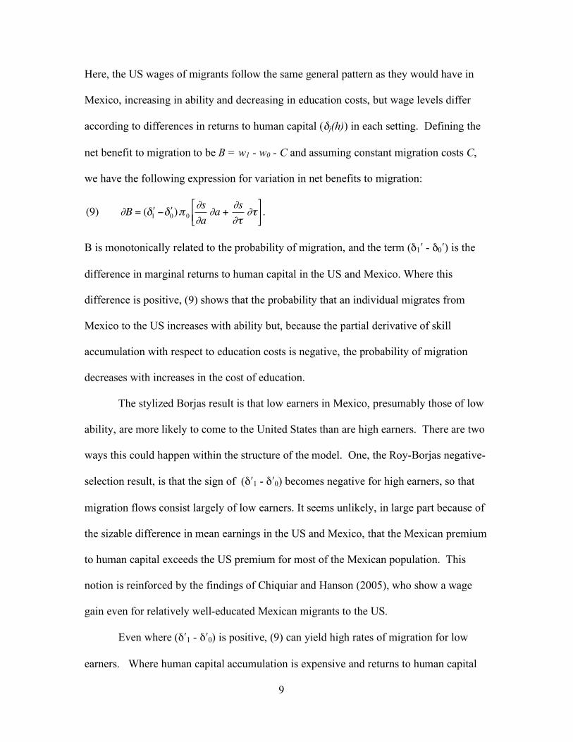
The distinguishing feature of our model is the explicit consideration of access to

education, $. Consider the impact of a change in Mexican schooling costs or ability, and

subsequent within-Mexico generation of human capital, on US earnings for migrants:

!

(7)"w

1

"#= $ %

1&0

"s

"# and

!

(8)"w

1

"a= # $

1%0

"s

"a .

9

Here, the US wages of migrants follow the same general pattern as they would have in

Mexico, increasing in ability and decreasing in education costs, but wage levels differ

according to differences in returns to human capital (!j(h)) in each setting. Defining the

net benefit to migration to be B = w1 - w0 - C and assuming constant migration costs C,

we have the following expression for variation in net benefits to migration:

!

(9) "B = ( # $ 1% # $

0)&

0

"s

"a"a +

"s

"'"'

(

) * +

, - .

B is monotonically related to the probability of migration, and the term (!1" - !0") is the

difference in marginal returns to human capital in the US and Mexico. Where this

difference is positive, (9) shows that the probability that an individual migrates from

Mexico to the US increases with ability but, because the partial derivative of skill

accumulation with respect to education costs is negative, the probability of migration

decreases with increases in the cost of education.

The stylized Borjas result is that low earners in Mexico, presumably those of low

ability, are more likely to come to the United States than are high earners. There are two

ways this could happen within the structure of the model. One, the Roy-Borjas negative-

selection result, is that the sign of (!"1 - !"0) becomes negative for high earners, so that

migration flows consist largely of low earners. It seems unlikely, in large part because of

the sizable difference in mean earnings in the US and Mexico, that the Mexican premium

to human capital exceeds the US premium for most of the Mexican population. This

notion is reinforced by the findings of Chiquiar and Hanson (2005), who show a wage

gain even for relatively well-educated Mexican migrants to the US.

Even where (!"1 - !"0) is positive, (9) can yield high rates of migration for low

earners. Where human capital accumulation is expensive and returns to human capital

10

are low at the destination, migration probabilities are low, all else constant. At the same

time, increasing ability is associated with increasing probabilities of migration, all else

constant. The question becomes one of the relative magnitudes of potentially opposing

effects. If the ability component dominates the accumulation component of the skill-

accumulation function s(a,"), as might occur with binding supply constraints in

education, and Mexican wages w0 are low enough compared to US wages,6 positive net

benefits of migration may obtain for those with low levels of human capital accumulation

but high levels of ability. While in some ways consistent with Borjas, in that educational

constraints make them low earners on arrival in the US, a broader, Roy-inspired

characterization of these individuals as being of low ability clearly would be

inappropriate in this case. Our model also allows for intermediate findings like those of

Chiquiar and Hanson, where the two effects yield a mix of migrants—those with some

human capital, either through native ability or training, are more likely to come to the US

than those without such capital.

An empirical model using Mexican data

The engine of Roy-Sjaastad migration is wage differentials. In Borjas’ (1999)

interpretation of the model for migration to the US from developing countries, the pull is

strongest for unskilled labor, and is posited to be the result of a relatively more diffuse

earnings distribution in Mexico. By migrating to the US, even though they remain at the

bottom of the US income distribution, they place themselves in the left tail of more

compact income distribution. The evidence in favor of this claim is largely

circumstantial, consisting of examining educational attainments or labor market outcomes

6 In this respect, the model is somewhat like that of Card’s (2001), where individual heterogeneity in the

marginal cost of education plays a key role in determining educational attainment.

11

of migrants. In what is to our knowledge the only direct examination of migrants’

placement in the sending country earnings distribution, Chiquiar and Hanson (2005)

provided strong evidence that, contrary to the prediction of negative self-selection, many

Mexicans solidly in the middle of the Mexican earnings distribution migrate to the US.

In this case, after Sjaastad, the driving force for migration is the difference in mean

wages between the US and Mexico, and the case that migrants are of low quality is

weakened.

There are distinctly different roles played by human capital accumulation in

various iterations of the Roy-Sjaastad model. Where the focus is on variation in earnings,

as in the work of Borjas, increases in Mexican human capital move potential migrants

closer to mean Mexican earnings, and so render them less likely to migrate. Where the

focus is on the level of earnings, as in Chiquiar and Hanson, or more generally where

positive selection of migrants with increasing human capital across the spectrum of

earnings is allowed, increases in human capital lead to increases in migration

probabilities. The sign and magnitude of the effect of human capital on migration

probabilities therefore provides a simple and direct test of the competing hypotheses.

To examine the behavior we posit, we need to differentiate between baseline

ability (a) and skill accumulation (s). Fortunately for our purposes, access to education,

and so the cost of skill accumulation, varies widely within Mexico. Education through at

least high school is easily available in urban areas, but educational access is severely

constrained in rural areas, especially in the south. We treat these variations between

geographic areas as exogenously determined with regard to international migration, and

so interpret geographic differentials in educational attainment as the outcomes of natural

12

experiments, presumably based on variation in education funding. Our empirical strategy

is to control for varying costs of human capital attainment by assuming that public

resources allocated to education are constant within small geographic areas, so that each

individual within an area is subject to the same education funding constraint. We then are

able to interpret differences in educational attainment within these small areas as

reflective of ability, motivation and other innate differences in human capital, holding

cost of educational attainment constant.

The Mexican Migration Project surveyed households in a large number of

communities in Mexico7. The survey inquired of household members about other,

potentially migrant, members and so avoided the problem of interviewing only those who

reside in Mexico at the time of the survey. For all household members, including adult

children not currently resident, general demographic information and brief migration

measures were collected. Data included age, sex, relationship to head of household,

marital status, current economic indicators, and characteristics of the first and last trips

made to the US or to other Mexican locations. There also were detailed event histories

for each household head, including up to 25 border crossings, and for his or her spouse.

The survey was administered during the winter months surrounding the Christmas

holidays, in an effort to capture those migrants who live most of the year in the U.S. and

returned to Mexico for the holidays. The resulting dataset has information from 71

communities for over 83,000 individuals, roughly one-fifth of whom had US migration

experience. Data collection began in 1982, and we use information collected between

1982 and 1999. The unit of analysis is the individual, and each surveyed household can

contribute multiple observations. Those individuals who had their first migration

7 See Massey et al. 1994 for a more complete description of these data.

13

experience prior to age 15 were dropped, as they were not likely to have engaged in an

independent choice to migrate.8

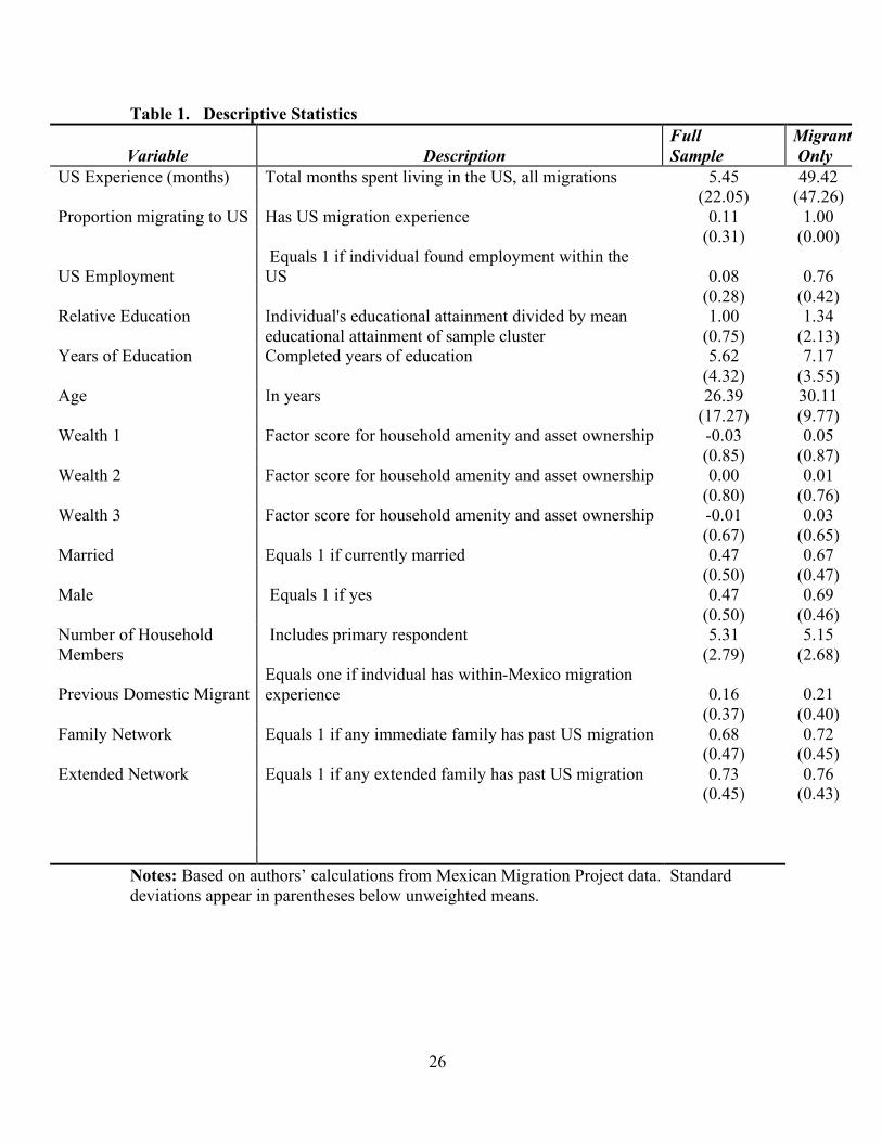
Summary statistics are presented in table 1. The variables are largely self-

explanatory, with the possible exceptions of relative education and the wealth variables.

The wealth variables are three factor scores based on a set of thirteen selected indicators

of wealth or financial wellbeing9. We take the factor score approach because the thirteen

indicators of wealth we employ are likely to be highly correlated with one another. Using

factor scores allows us to preserve as much information from these variables as we can,

and so, we hope, credibly to control for wealth variation in the regressions we run. There

are three scores that result from the factor analysis of the thirteen underlying indicators of

wealth. It is immediately apparent that compared to the full sample, which consists

largely of nonmigrants, US migrants are better educated, in both absolute and relative

terms; somewhat older, slightly less wealthy than average, and more likely to be male.

(Table 1 here)

The key variable in our analysis is relative educational attainment. In poor

communities, the mean number of years of school attended was low—the value for the

33rd

percentile of educational attainment over the entire sample was 4.29 years—and

someone who had more than this level of educational attainment could be construed, in

relative terms for that community, to be reasonably well educated. Geographic mobility

of children, especially in rural areas, is limited, and so differentials in local education

funding levels are likely to be persistent over their youth. Therefore, cross-sectional

8 This restriction is costly, as it eliminates almost half of the sample of US migrants.

9 The variables are dummies for ownership of land; a stove, refrigerator, washing machine, sewing

machine, radio, television, stereo, telephone, or motor vehicle, and whether the respondent’s dwelling has

running water, electricity, and flush toilets.

14

variation in educational attainment over the entire sample represents the impact of a

combination of supply side constraints, shared by all in a locality, and individual

variations in aptitude, motivation, and so forth.

We have two concerns regarding the use of this variable as a proxy for ability.

First, relative education is calculated based on the community of residence for the

respondent at the time of the survey, but its theoretical justification rests on constraints

operating during childhood and adolescence. Domestic rural to urban migration is fairly

common, and this may lead to some measurement error in relative education. Where this

occurs, the relative education we calculate is based on urban means. Because this is an

understatement of the true relative education for the rural area of origin, we expect that

internal migration will bias our results in the direction of conservatism.

Our analysis rests on the claim that relative education or motivation reflects

underlying ability more accurately than does overall years of education attained, because

it measures educational attainment in the context of local supply constraints. We will

interpret a positive marginal effect of relative education as evidence of positive migrant

selection based upon ability, and the converse as evidence of negative selection. The

validity of this claim depends on the degree to which relative educational attainment

reflects merit over (local) privilege. Our second concern is that relative educational

attainment probably is a noisy proxy for ability, so that, after the standard measurement

error result, we once again are likely to underestimate its effect. The problem may be

more severe than simple noise. For example, a more systematic effect may occur if the

locally privileged have both easier access to education and reduced likelihood of leaving

a comfortable situation. In this case, we are probably again underestimating the true

15

impact of relative education, biasing our result by including those who have high levels

of relative education but with (potentially) low levels of ability and low probabilities of

leaving home. While in either case, the estimated effect of relative education is likely to

be conservatively estimated, we recognize that there may be sources of bias that operate

to overstate the impact of relative education on migration propensities.

Reflecting the importance of educational attainment as a measure of quality in the

literature, we include total years of education attained as a covariate. We include several

demographic measures, including age, marital status, and sex. We also include several

indicators of resource availability and costs of migration, including family size and three

measures of wealth. Three proxies for the availability of migration networks and

opportunity costs appear as dummy variables: whether the individual had migrated

domestically, and whether they had immediate family or extended family in the United

States.

We estimate several models, regressed on a common set of covariates. All

incorporate community-level fixed-effects. Our contention that community-level

constraints in the supply of education exist is key to our argument, and our purpose in

including community-level fixed effects is twofold. First, we want to capture other

sources of community-level variation than levels of education. Secondly, we want to use

Hausman specification tests on models that omit and include relative education as a

means of assessing in a fairly general way the importance of community level differences

in access to education in subsequent migration outcomes. The first model is a linear

regression model on months spent in the United States, with a sample including both

migrants and non-migrants. Never-migrants have a value of zero for the dependent

16

variable, and the sum of all months spent in the US is recorded for migrants. The

information contained in the dependent variable for this regression therefore is a mixture

of migration propensities and durations of stay. We estimate this and subsequent models

for a full sample, and separately for subsamples of male and female respondents.

We attempt to decompose variation in the dependent variable of this simple model

into its constituent parts in two subsequent regressions. First, we estimate the

determinants of migration probability. A respondent is designated as a migrant if they

have reported one or more total months of US migration experience.10

Presumably, an

important determinant of how long a migrant stays is his or her success in the US labor

market. We next estimate linear models of the probability that a migrant found

employment in the US on their last or current migration. The independent variable here is

created from a categorical variable that classifies occupations held by migrants on their

last trip to the US. Overall, approximately seventy-seven percent of all migrants were

employed during their last migration to the US11

. Only the migrant subsample is used to

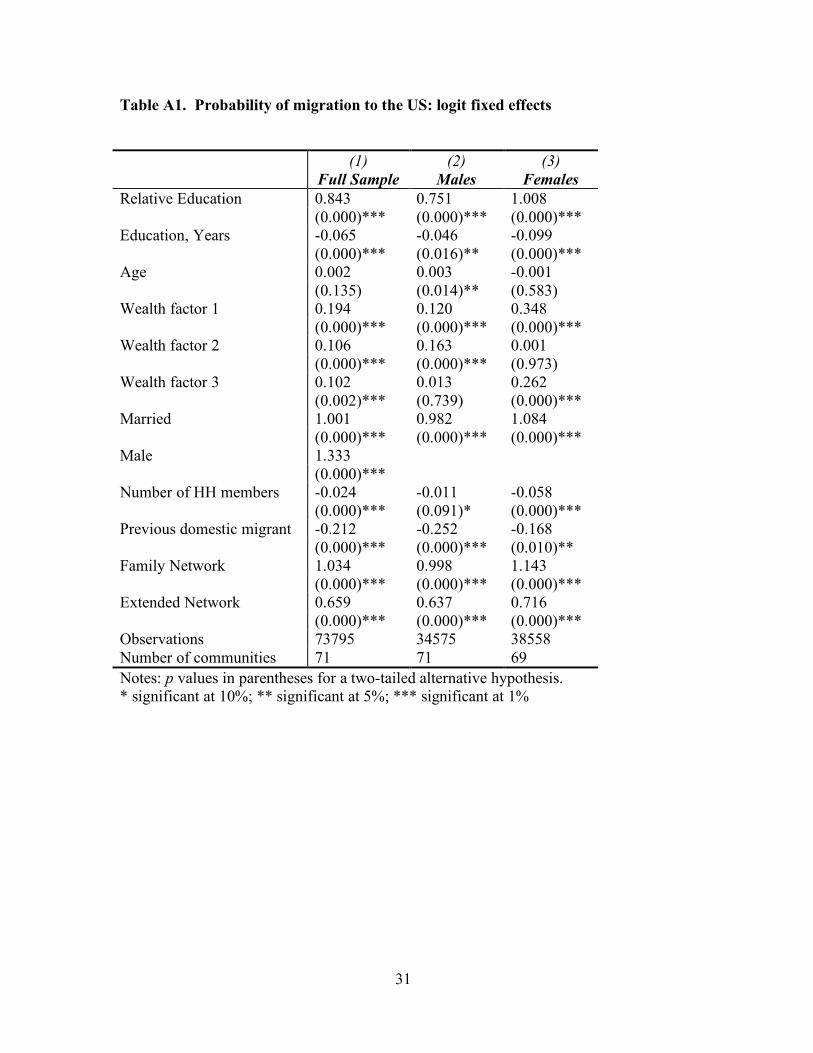
estimate this equation. We estimate both of these models as conditional community-level

fixed-effects logits, and, because of the difficulty of calculating marginal effects for this

type of model, as linear probability models with community-level fixed effects. We

present the fixed-effects logit results in the appendix. Because there are no striking

inferential differences between the logit and linear probability models, we focus on the

marginal effects from the linear probability results in the text.

(Table 2 here)

10

Within our sample, there are fifty-three individuals that report at least one migration to the US but who

also report having less than one month of US migration experience. They are not counted as migrants in

our analysis. 11

Some of these migrants may still be in the US at the time of the interview.

17

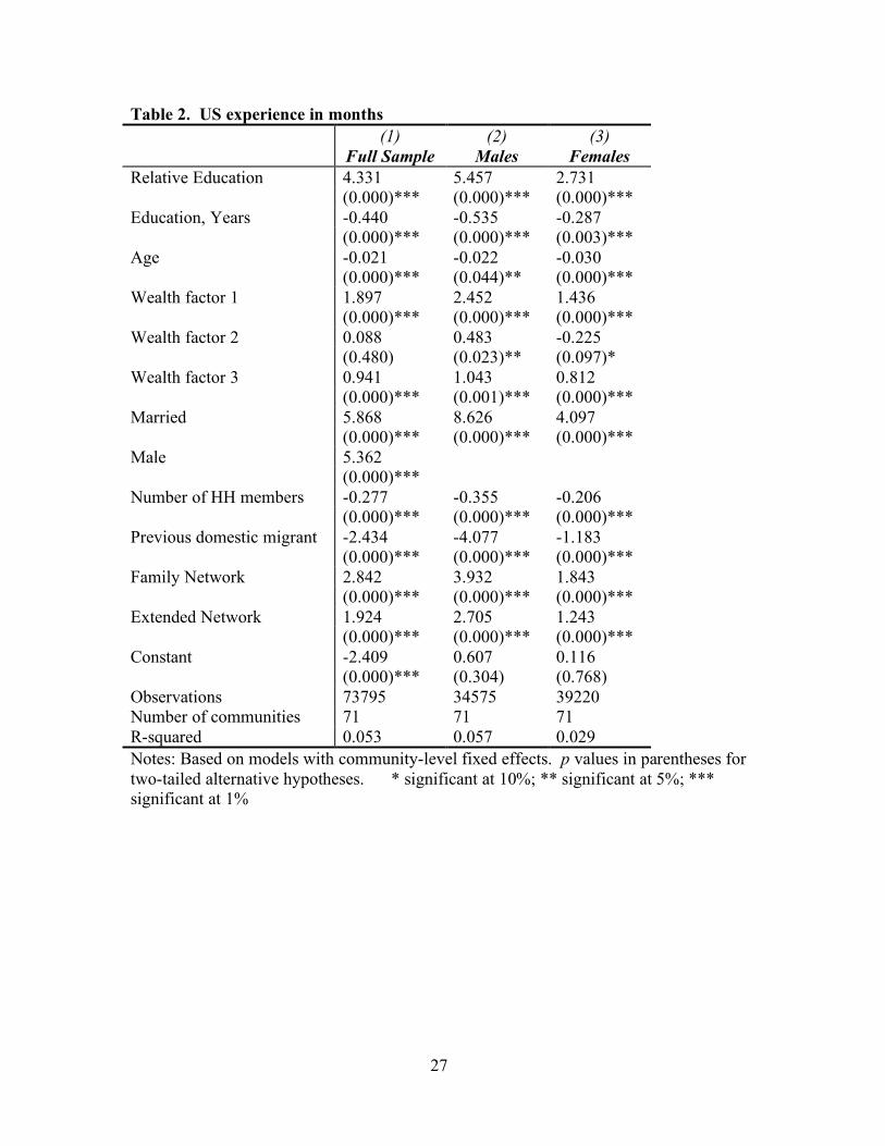
Table 2 shows that both education variables have distinct impacts on the linear

regression for total months in the US. The coefficient of relative education is positive

and significant in all cases. For the full sample, its value of 4.331 implies that the mean

months spent living in the US for this group, 5.45 months, would be increased to 8.6

months by a one standard deviation (0.75) increase in relative education. Absolute

education decreases average durations in the US. For the full sample, a one standard

deviation increase in education (4.3 years) would decrease duration in the US to 3.5

months. The effect of education, either relative or absolute, is roughly twice as large for

men as women, and the coefficient of “Male” shows that men, on average, stayed more

than five months longer in the US than did women on their last migration to the US.

The control variables in these results have coefficients much as expected.

Younger people are either more likely to go to the US or likely to stay longer than older

people, all else constant. We confirm the contention of Chiquiar and Hanson (2005) that

those from wealthier households are more likely to come or to stay in the US. A male

from a household one standard deviation above the mean in each wealth category spent

3.1 more months in the US, all else constant, than someone from a household with

average wealth. Married individuals, especially men, are more likely to spend time in the

US. Those who have migrated previously within Mexico are less likely to have spent

time in the US, and those with migration networks in place are more likely to have spent

time in the US than those without such networks.

The unanswered question from these results is whether variations in duration in

the US are due to changes in the probability that an individual migrates to the US in the

first place, or to changes in duration or in the probability that he or she stays in the US.

18

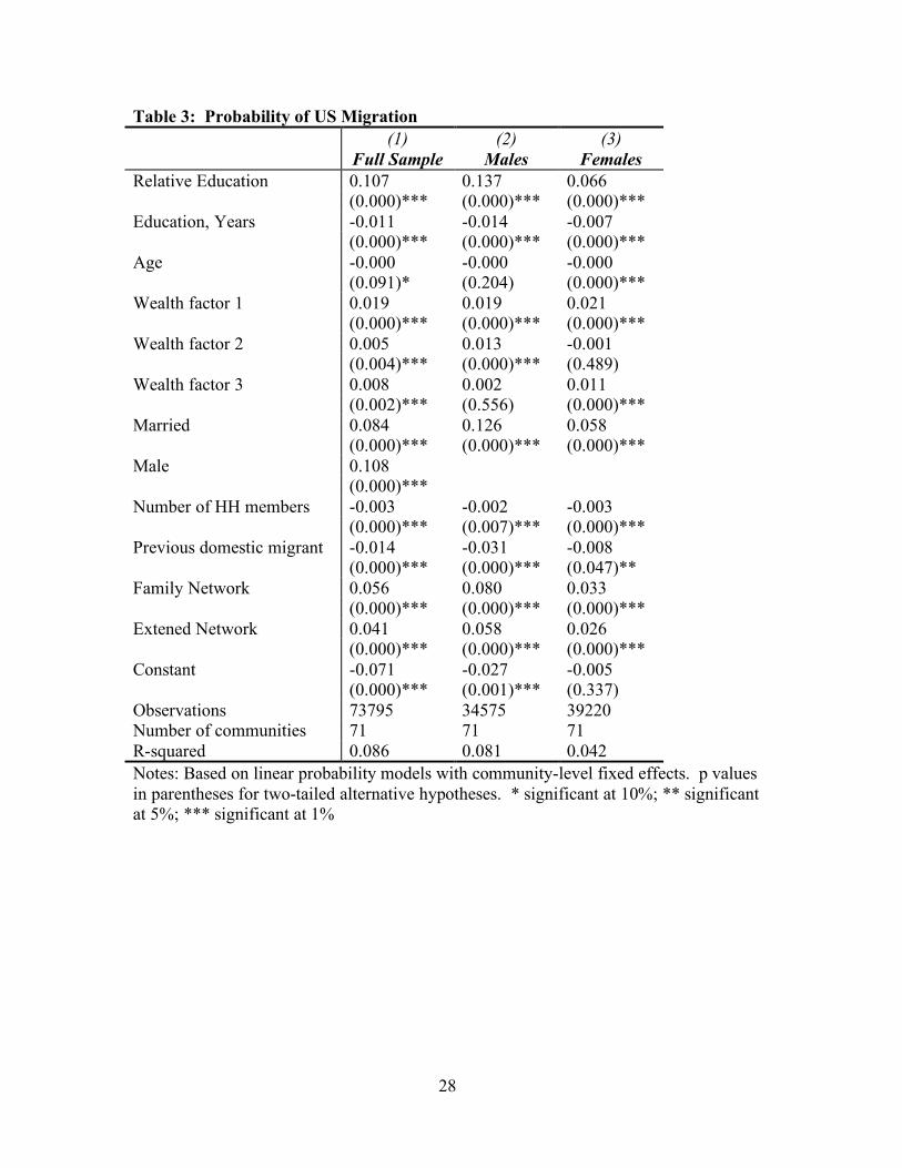
As the first step in decomposing the gross “US months” effect, we estimate a model of

the probability of ever having migrated to the US, and present the results in Table 3. The

determinants of migration are similar to those for total months in the US. Strikingly,

those relatively better educated are more likely to have migrated to the US at least once,

but those absolutely better educated are less likely to have done so. For males, we

estimate that all else constant, being one standard deviation above mean relative

education increases the probability of migrating by just over 10 points, or roughly double

the mean of 11%. Age is not an important determinant of US migration, but those from

wealthier households and with access to migration networks display higher probability of

ever migrating.

It is instructive to compare the magnitudes of the education effects in two stylized

settings. In the first, comparable to rural southern Mexico, adults average four years of

education completed. In the second, as might be the case in an urban area like Mexico

City, adults average ten years of completed education. Consider someone with eight

completed years of education. If they lived in the rural area, they would have relative

education of 2.0; in the urban, relative education of 0.8. An otherwise average male with

eight years of education has a predicted probability of migrating to the US from the

stylized rural area of 0.20, and from the stylized urban area of 0.04. Those with less

overall education therefore are much more likely to migrate to the US, as predicted by

Borjas. However, this result masks the subtler underlying finding that it is potentially

high-ability individuals from educationally supply-constrained areas who account for

much of this migration.

(Table 3 here)

19

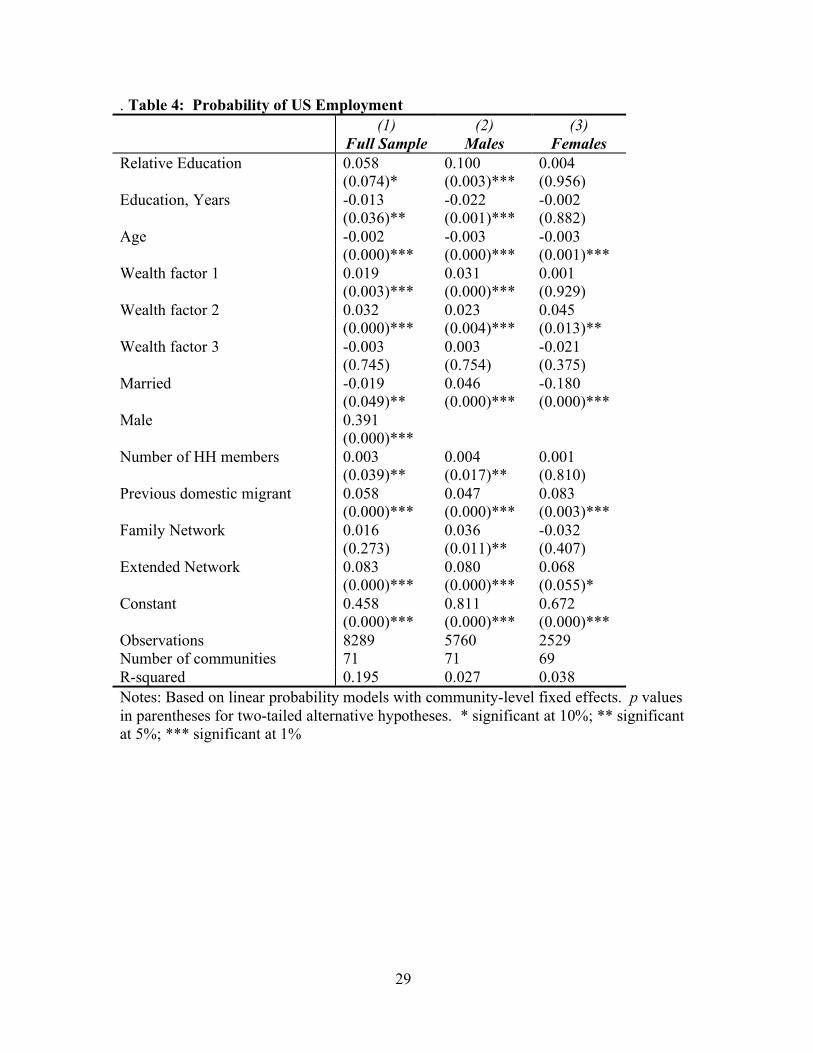
Given that migrants come to the US, the key question regarding how long they

stay is how they fare in the labor market. For the subsample of migrants to the US, we

estimated models of the probability of obtaining US employment. Focusing on the

results for males for the moment, Table 4 shows that, again, those with relatively high

education for the sending area do better in the job market. Of all male migrants to the US

in our sample, 87% reported finding a job in the US. A one standard deviation increase

in relative education increases this by 7.5 points, an increase of roughly 8.6%. This

effect would be offset by an increase of about 5 years in absolute education. Considering

again the stylized male migrants, each with 8 years of education but otherwise at sample

averages, we estimate the probability that the migrant from the education-constrained

area works at a job in the US to be 0.80, and from the area with higher levels of

education, 0.68.12

Finally, Table 4 shows little in the way of systematic determinants of

female employment. Most notable is the large negative coefficient for married women,

suggesting that some women are accompanying spouses but not entering the labor market

themselves.

(Table 4 here)

If educational constraints operating at the community level are important sources

of community level variation, their omission from the models we have examined should

be statistically costly. Our approach will be to exploit the well-known inconsistency of

random-effects estimators in the presence of omitted community-level variables when

these variables are correlated with included variables. We estimate models that

completely omit education; that include only absolute years of education; that include

12

We note that in this example, the coefficient of years of education is sufficiently negative for an above-

average level of education to generate predictions that in both cases are below sample averages.

20

only relative education, and that include both measures of education, in every case

including the full remaining set of control variables we have been using. We estimate

each in turn with a random effects estimator and a fixed effects estimator, exploiting the

consistency of the fixed-effects estimator to construct standard Hausman tests of the null

hypothesis that the random effects estimator is consistent. If, in moving from models that

ignore education to models that include it, we fail to reject the null hypothesis, this

constitutes support for the notion that the additional variables capture important variation

in outcomes.

(Table 5 here)

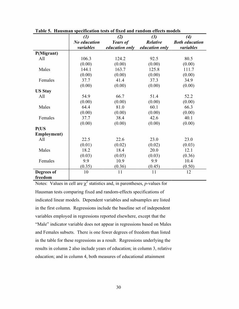
Table 5 presents a set of &2 statistics and associated p-values for various

regression models. The three dependent variables and three subsets of cases used in

Tables 2-4 appear in the rows of Table 5. The columns of Table 5 list the four

permutations of models just described. For the regressions of migrant and US stay, the

null hypothesis invariably is rejected. This must be construed as evidence that there

remain community-level effects not captured in the model, even after the educational

attainment variables are added. While the regression results in Tables 2 and 3 show the

education variables, especially relative education, to be important determinants of the

decision to migrate, the Hausman tests suggest that there are other community-level

effects not explicitly captured in the model that matter as well.

The determinants of the probability of US employment regressions are not

estimated precisely for female migrants, in part because the sample is relatively small,

but in part for reasons we have discussed above. In the US employment results of table

5, our focus therefore will be on males. In the final column, with the addition of

21

community-level and absolute years of education, we fail to reject the null hypothesis that

the random-effects model is consistent for males. This is supportive of the notion that

differences in educational attainment, both relative and absolute, are important

community-level sources of variation in accounting for US employment of migrants.

Notably, it takes both measures of educational attainment to achieve this result,

suggesting that the true effect of relative education on US employment of migrants may

be somewhat subtler than the simple linear specification we employ.

Discussion

We have developed a model of migration driven by human capital accumulation

where, in typical fashion, human capital consists of an endowment of ability and an

accumulation of skills. Though very simple, it is sufficient to generate two cases of

interest. In the first, which is essentially the Borjas (1999) interpretation of Roy (1951),

US earnings premiums drive those at the low end of the Mexican earnings scale to

migrate to the US. To be a credible explanation of migration concentrated amongst low-

skill immigrants, it must be the case that US wage premiums are relatively higher for less

educated than for more educated. Evidence on whether this is the case is mixed at best,

and Chiquiar and Hanson (2005) present the convincing counterpoint that mean earnings

are sufficiently high in the US that many across the Mexican income spectrum have an

incentive to migrate. In the second case, to the extent that Mexican migrants possess low

human capital, the explanation within our model is that they are high-ability individuals

who have been constrained in obtaining education.

Our findings are in many ways consistent with Borjas’. Borjas finds that

immigrants have low absolute levels of education, and we confirm that, at least when

22

compared to native US workers13

. Borjas finds that migrants are more likely to come

from countries with higher degrees of income inequality, and we indirectly extend this to

the subnational level, as those from areas with lower average levels of education are more

likely to migrate to the US than are individuals from areas where education level are

higher. Our differences with models reporting negative self-selection of migrants to the

US emerge as we look more closely at measures of immigrant quality.

Most notably, Mexicans with more relative education are more likely to migrate

to the United States and to find employment when they arrive than those with less

relative education. Those with more absolute education are less likely to migrate to the

United States than the more educated, though this effect is swamped by the relative

education effect, and less likely to get a job in the US. Therefore, we attribute a

significant share of the low levels of education Mexican migrants to the United States

display to supply constraints operating in their origin localities. To the extent that

increasing relative education captures increases in traits like ability or motivation, it is

apparently the more motivated or innately able that are migrating to the US. The findings

of Schoeni (1997) and Card (2005) on the labor market advantages enjoyed by migrants’

children are consistent with the notion that the migrants themselves are of high innate

ability. The Borjas result that those from sending countries where income is more

unequally distributed are more likely to come to the US also is consistent with our result,

as those are the countries of origin from which immigrants of high ability, faced with

constraints in obtaining education at home, have the most to gain by immigrating to the

US. The causal mechanism we propose clearly is somewhat different than that offered by

13

However, like Chiquiar and Hanson (2005), we find that on average, migrants to the US have more

education than nonmigrants.

23

Borjas. Because we have fairly direct evidence on the mechanics of the process, we do

not view Borjas’ results as especially persuasive evidence of negative selection of

immigrants.

The policy implications of our findings are very different from those that emerge

from analyses where migrant quality is approximated by years of education or, by

extension, labor market outcomes of immigrants. In the absence of supply constraints,

years of completed education may well be a reasonable proxy to assess both human

capital stocks and ability levels of immigrants. On the other hand, if, as appears to be the

case in much of Mexico, educational attainment is supply constrained, completed years of

education is flawed as a measure both of the entry-level stock of human capital and the

possible trajectory of human capital over time, because the low levels of education we

observe causes us to undervalue the ability component of human capital.

It seems from our results that educational supply constraints operate in Mexico,

and that (relatively) able but (absolutely) poorly educated immigrants are self-selecting

from poorer regions of Mexico. It is likely that Mexico represents the rule rather than an

exception amongst developing countries in this regard. If so, observed United States labor

market differentials may actually reflect educational supply constraints in sending

countries that have the effect of masking relatively high underlying ability of immigrants.

Models of negative selection are often used to justify reducing the number of immigrants

from particular origins. Rather than tightly restricting immigration, a case can be made

from the present results and those of and Chiquiar and Hanson (2005) for an immigration

policy that contains a significant training component, potentially easing the transition into

the United States economy for relatively able but untrained migrants.

24

References

Borjas, George J. 1990. Friends or Strangers: The Impact of Immigrants on the US

Economy. New York: Basic Books.

Borjas, George J. 1991. Ethnic Capital and Intergenerational Mobility. Quarterly

Journal of Economics 107,1 (February): 123-150.

Borjas, George J. 1994. The Economics of Immigration. Journal of Economic Literature

32 (4): 1667-1717.

Borjas, George J. 1999. Heaven’s Door: Immigration Policy and the American

Economy. Princeton: Princeton University Press.

Card, David. 2001. Estimating the Returns to Schooling: Progress on some Persistent

Economic Problems. Econometrica 69, no. 5 (Sept.): 1127-1160.

Card, David. 2005. Is the New Immigration Really So Bad? The Economic Journal

115, no. 507: F300-F323

Chiquiar, David and Gordon Hanson. 2005. International Migration, Self-Selection, and

the Distribution of Wages: Evidence from Mexico and the United States. Journal

of Political Economy 113: 239–281.

Chiswick, Barry R. 1999. Are Immigrants Favorably Self-Selected? An Economic

Analysis. American Economic Review 89, no. 2 (May):181-185.

Duleep, Harriet Orcutt and Mark C. Regets. 1999. Immigrants and Human Capital

Investment. American Economic Review 89, no. 2 (May): 186-191.

Massey, Douglas S., Joaquin Arango, Ali Koucouci, Adela Pelligrino, and J. Edward

Taylor. 1994. An Evaluation of International Migration Theory: The North

American Case. Population and Development Review 20: 699-752.

25

Roy, Andrew D. 1951. “Some Thoughts on the Distribution of Earnings,” Oxford

Economic Papers 3: 135-146.

Schoeni, Robert F. 1997. New Evidence on the Economic Progress of Foreign-Born Men

in the 1970s and 1980s. The Journal of Human Resources 32, no. 4. (Autumn):

683-740.

Sjaastad, Larry A. 1962. “The costs and returns of human migration”, Journal of

Political Economy 70 (Supplement): 80-93.

Stark, Oded and J. Edward Taylor. Migration Incentives, Migration Types: The Role of

Relative Deprivation. Economic Journal 101, no. 408 (September): 1163-1178.

26

Table 1. Descriptive Statistics

Variable Description

Full

Sample

Migrants

Only

US Experience (months) Total months spent living in the US, all migrations 5.45 49.42

(22.05) (47.26)

Proportion migrating to US Has US migration experience 0.11 1.00

(0.31) (0.00)

US Employment

Equals 1 if individual found employment within the

US 0.08 0.76

(0.28) (0.42)

Relative Education Individual's educational attainment divided by mean 1.00 1.34

educational attainment of sample cluster (0.75) (2.13)

Years of Education Completed years of education 5.62 7.17

(4.32) (3.55)

Age In years 26.39 30.11

(17.27) (9.77)

Wealth 1 Factor score for household amenity and asset ownership -0.03 0.05

(0.85) (0.87)

Wealth 2 Factor score for household amenity and asset ownership 0.00 0.01

(0.80) (0.76)

Wealth 3 Factor score for household amenity and asset ownership -0.01 0.03

(0.67) (0.65)

Married Equals 1 if currently married 0.47 0.67

(0.50) (0.47)

Male Equals 1 if yes 0.47 0.69

(0.50) (0.46)

Number of Household Includes primary respondent 5.31 5.15

Members (2.79) (2.68)

Previous Domestic Migrant

Equals one if indvidual has within-Mexico migration

experience 0.16 0.21

(0.37) (0.40)

Family Network Equals 1 if any immediate family has past US migration 0.68 0.72

(0.47) (0.45)

Extended Network Equals 1 if any extended family has past US migration 0.73 0.76

(0.45) (0.43)

Notes: Based on authors’ calculations from Mexican Migration Project data. Standard

deviations appear in parentheses below unweighted means.

27

Table 2. US experience in months

(1)

Full Sample

(2)

Males

(3)

Females

Relative Education 4.331 5.457 2.731 (0.000)*** (0.000)*** (0.000)***

Education, Years -0.440 -0.535 -0.287 (0.000)*** (0.000)*** (0.003)***

Age -0.021 -0.022 -0.030 (0.000)*** (0.044)** (0.000)***

Wealth factor 1 1.897 2.452 1.436 (0.000)*** (0.000)*** (0.000)***

Wealth factor 2 0.088 0.483 -0.225 (0.480) (0.023)** (0.097)*

Wealth factor 3 0.941 1.043 0.812 (0.000)*** (0.001)*** (0.000)***

Married 5.868 8.626 4.097 (0.000)*** (0.000)*** (0.000)***

Male 5.362

(0.000)***

Number of HH members -0.277 -0.355 -0.206 (0.000)*** (0.000)*** (0.000)***

Previous domestic migrant -2.434 -4.077 -1.183 (0.000)*** (0.000)*** (0.000)***

Family Network 2.842 3.932 1.843 (0.000)*** (0.000)*** (0.000)***

Extended Network 1.924 2.705 1.243 (0.000)*** (0.000)*** (0.000)***

Constant -2.409 0.607 0.116 (0.000)*** (0.304) (0.768)

Observations 73795 34575 39220

Number of communities 71 71 71

R-squared 0.053 0.057 0.029

Notes: Based on models with community-level fixed effects. p values in parentheses for

two-tailed alternative hypotheses. * significant at 10%; ** significant at 5%; ***

significant at 1%

28

Table 3: Probability of US Migration

(1)

Full Sample

(2)

Males

(3)

Females


Education, Years -0.011 -0.014 -0.007 (0.000)*** (0.000)*** (0.000)***

Age -0.000 -0.000 -0.000 (0.091)* (0.204) (0.000)***

Wealth factor 1 0.019 0.019 0.021 (0.000)*** (0.000)*** (0.000)***

Wealth factor 2 0.005 0.013 -0.001 (0.004)*** (0.000)*** (0.489)

Wealth factor 3 0.008 0.002 0.011 (0.002)*** (0.556) (0.000)***

Married 0.084 0.126 0.058 (0.000)*** (0.000)*** (0.000)***

Male 0.108

(0.000)***

Number of HH members -0.003 -0.002 -0.003 (0.000)*** (0.007)*** (0.000)***

Previous domestic migrant -0.014 -0.031 -0.008 (0.000)*** (0.000)*** (0.047)**

Family Network 0.056 0.080 0.033 (0.000)*** (0.000)*** (0.000)***

Extened Network 0.041 0.058 0.026 (0.000)*** (0.000)*** (0.000)***

Constant -0.071 -0.027 -0.005 (0.000)*** (0.001)*** (0.337)



R-squared 0.086 0.081 0.042

Notes: Based on linear probability models with community-level fixed effects. p values

in parentheses for two-tailed alternative hypotheses. * significant at 10%; ** significant

at 5%; *** significant at 1%

29

. Table 4: Probability of US Employment

(1)

Full Sample

(2)

Males

(3)

Females

Relative Education 0.058 0.100 0.004 (0.074)* (0.003)*** (0.956)

Education, Years -0.013 -0.022 -0.002 (0.036)** (0.001)*** (0.882)

Age -0.002 -0.003 -0.003 (0.000)*** (0.000)*** (0.001)***

Wealth factor 1 0.019 0.031 0.001 (0.003)*** (0.000)*** (0.929)

Wealth factor 2 0.032 0.023 0.045 (0.000)*** (0.004)*** (0.013)**

Wealth factor 3 -0.003 0.003 -0.021 (0.745) (0.754) (0.375)

Married -0.019 0.046 -0.180 (0.049)** (0.000)*** (0.000)***

Male 0.391

(0.000)***

Number of HH members 0.003 0.004 0.001 (0.039)** (0.017)** (0.810)

Previous domestic migrant 0.058 0.047 0.083 (0.000)*** (0.000)*** (0.003)***

Family Network 0.016 0.036 -0.032 (0.273) (0.011)** (0.407)

Extended Network 0.083 0.080 0.068 (0.000)*** (0.000)*** (0.055)*

Constant 0.458 0.811 0.672 (0.000)*** (0.000)*** (0.000)***



R-squared 0.195 0.027 0.038

Notes: Based on linear probability models with community-level fixed effects. p values

in parentheses for two-tailed alternative hypotheses. * significant at 10%; ** significant

at 5%; *** significant at 1%

30

Table 5. Hausman specification tests of fixed and random effects models

(1)

No education

variables

(2)

Years of

education only

(3)

Relative

education only

(4)

Both education

variables

P(Migrant)

All 106.3

(0.00)

124.2

(0.00)

92.5

(0.00)

80.5

(0.00)

Males 144.1

(0.00)

163.7

(0.00)

125.8

(0.00)

111.7

(0.00)

Females 37.7

(0.00)

41.4

(0.00)

37.3

(0.00)

34.9

(0.00)

US Stay

All 54.9

(0.00)

66.7

(0.00)

51.4

(0.00)

52.2

(0.00)

Males 64.4

(0.00)

81.0

(0.00)

60.1

(0.00)

66.3

(0.00)

Females 37.7

(0.00)

38.4

(0.00)

42.6

(0.00)

40.1

(0.00)

P(US

Employment)

All 22.5

(0.01)

22.6

(0.02)

23.0

(0.02)

23.0

(0.03)

Males 18.2

(0.03)

18.4

(0.05)

20.0

(0.03)

12.1

(0.36)

Females 9.9

(0.35)

10.9

(0.36)

9.9

(0.45)

10.4

(0.50)

Degrees of

freedom

10 11 11 12

Notes: Values in cell are !2 statistics and, in parentheses, p-values for

Hausman tests comparing fixed and random-effects specifications of

indicated linear models. Dependent variables and subsamples are listed

in the first column. Regressions include the baseline set of independent

variables employed in regressions reported elsewhere, except that the

“Male” indicator variable does not appear in regressions based on Males

and Females subsets. There is one fewer degrees of freedom than listed

in the table for these regressions as a result. Regressions underlying the

results in column 2 also include years of education; in column 3, relative

education; and in column 4, both measures of educational attainment

31

Table A1. Probability of migration to the US: logit fixed effects

(1)

Full Sample

(2)

Males

(3)

Females


Education, Years -0.065 -0.046 -0.099 (0.000)*** (0.016)** (0.000)***

Age 0.002 0.003 -0.001 (0.135) (0.014)** (0.583)

Wealth factor 1 0.194 0.120 0.348 (0.000)*** (0.000)*** (0.000)***

Wealth factor 2 0.106 0.163 0.001 (0.000)*** (0.000)*** (0.973)

Wealth factor 3 0.102 0.013 0.262 (0.002)*** (0.739) (0.000)***

Married 1.001 0.982 1.084 (0.000)*** (0.000)*** (0.000)***

Male 1.333

(0.000)***

Number of HH members -0.024 -0.011 -0.058 (0.000)*** (0.091)* (0.000)***

Previous domestic migrant -0.212 -0.252 -0.168 (0.000)*** (0.000)*** (0.010)**

Family Network 1.034 0.998 1.143 (0.000)*** (0.000)*** (0.000)***




Notes: p values in parentheses for a two-tailed alternative hypothesis.

* significant at 10%; ** significant at 5%; *** significant at 1%

32

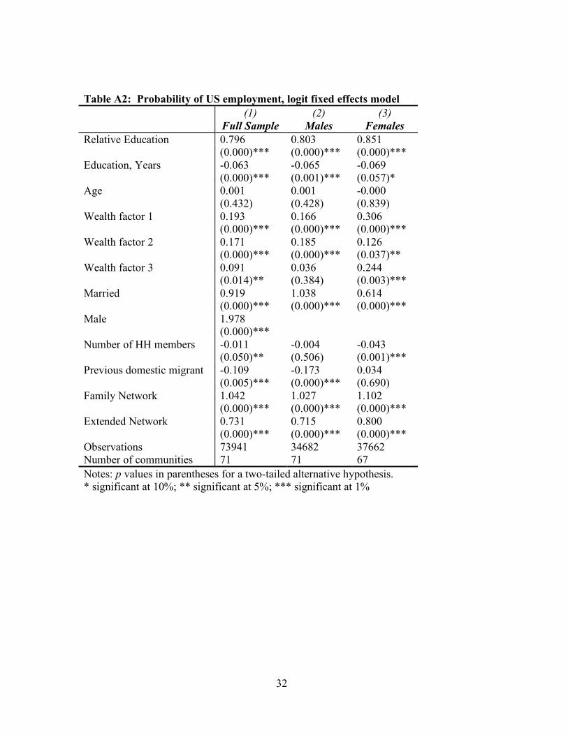
Table A2: Probability of US employment, logit fixed effects model

(1)

Full Sample

(2)

Males

(3)

Females


Education, Years -0.063 -0.065 -0.069 (0.000)*** (0.001)*** (0.057)*

Age 0.001 0.001 -0.000 (0.432) (0.428) (0.839)

Wealth factor 1 0.193 0.166 0.306 (0.000)*** (0.000)*** (0.000)***

Wealth factor 2 0.171 0.185 0.126 (0.000)*** (0.000)*** (0.037)**

Wealth factor 3 0.091 0.036 0.244 (0.014)** (0.384) (0.003)***

Married 0.919 1.038 0.614 (0.000)*** (0.000)*** (0.000)***

Male 1.978

(0.000)***

Number of HH members -0.011 -0.004 -0.043 (0.050)** (0.506) (0.001)***

Previous domestic migrant -0.109 -0.173 0.034 (0.005)*** (0.000)*** (0.690)

Family Network 1.042 1.027 1.102 (0.000)*** (0.000)*** (0.000)***




Notes: p values in parentheses for a two-tailed alternative hypothesis.

* significant at 10%; ** significant at 5%; *** significant at 1%

on migrant selectivity eric r. jensen college of william ...economics.wm.edu/wp/cwm_wp32.pdf · on...

Documents