on log-normal convolutions: an analytical-numerical method ...math.yorku.ca/~dhackman/log.pdf · on...
TRANSCRIPT

Electronic copy available at: https://ssrn.com/abstract=3034540
On log-normal convolutions: An analytical-numerical method
with applications to economic capital determination
Edward Furman∗, Dan Hackmann†, Alexey Kuznetsov‡
September 5, 2017
Abstract
We put forward an efficient algorithm for approximating the sums of independent and log-
normally distributed random variables. Namely, by merging tools from probability theory and nu-
merical analysis, we are able to compute the cumulative distribution functions of the just-mentioned
sums with any desired precision. Importantly, our algorithm is fast and can tackle equally well sums
with just a few or thousands of summands. We illustrate the effectiveness of the new method in
the contexts of the individual and collective risk models, aggregate economic capital determination,
and economic capital allocation.
Keywords: log-normal distribution, convolution, generalized gamma convolution, Pade approximation,
individual risk model, collective risk model, economic capital
JEL Classification: C02, C46, C63
1 Introduction
The log-normal distribution has been found appropriate for modelling losses originating from a great
variety of non-life insurance risks (e.g., Mikosch, 2009; Klugman et al., 2012). More specifically, Kleiber
and Kotz (2003) mention applications in property, fire, hurricane, and motor insurances, to name just
a few (also, e.g., Dropkin, 1964; Bickerstaff, 1972; O’Neill and Wells, 1972). Furthermore the standard
∗Dept. of Mathematics and Statistics, York University, 4700 Keele Street, Toronto, ON, M3J 1P3, Canada. Email:
[email protected]†Institute of Financial Mathematics and Applied Number Theory, Johannes Kepler University, Linz, Austria. Email:
[email protected]‡Dept. of Mathematics and Statistics, York University, 4700 Keele Street, Toronto, ON, M3J 1P3, Canada. Email:
1

Electronic copy available at: https://ssrn.com/abstract=3034540
formula of the European Insurance and Occupational Pensions Authority explicitely assumes the log-
normality of insurers’ losses (EIOPA-14-322, 2014). Finally, the role of the log-normal distribution is
at least as profound in finance, where it serves as the canonical model describing stock price returns
(e.g., Sprenkle, 1964; Milevsky and Posner, 1998). For a multitude of applications of the log-normal
distribution in other areas we refer to Limpert et al. (2001), and references therein.
Recall that the random variable (r.v.) Xµ,σ is said to be distributed log-normally with parameters
µ ∈ (−∞,∞) and σ > 0, succinctly Xµ,σ ∼ LN(µ, σ2), if its probability density function (p.d.f.) is given
by
f(x) =1
x√
2πσ2exp
(−1
2
(ln(x)− µ
σ
)2)
for x > 0. (1)
Although Xµ,σ is merely a simple transform of the well-understood Gaussian r.v., it has been puzzling
researchers for decades. For instance, an explicit expression for the Laplace transform of (1) has eluded
mathematicians thus far, and the existing series representations are rather cumbersome (Leipnik, 1991).
In this paper we are interested in a related problem of log-normal convolutions. In fact, the convolu-
tions of log-normal distributions have drawn considerable attention of researchers and practitioners due
to the fundamental importance of log-normal sums in engineering, biology, ecology, and economics, as
well as in actuarial science and finance. It is not surprising therefore that the existing contributions on
the topic are abundant and span all of the just-mentioned areas (e.g., Dufresne, 2008; Asmussen et al.,
2011, for recent literature reviews).
The problem is admittedly very intricate, and no explicit solution is generally available. The existing
methods to approximate the log-normal convolutions can be associated with the following three main
threads, or their variants: (i) moment matching method and its modifications, (ii) series representations
of the Laplace transform, and (iii) asymptotic results.
The moment matching method is akin to the idea of approximating the convolutions of log-normal dis-
tributions by means of (other) distributions. It seems that for the first time this method was documented
in Fenton (1960), who employs the log-normal distribution with the first and second moments being equal
to the first and second moments of the desired log-normal sum (e.g., Beaulieu et al., 1995; Milevsky and
Posner, 1998). The idea is further refined in Chen et al. (2008) and Zhang and Song (2008), who utilize
the four-parameter Pearson IV family of distributions to approximate the distribution of log-normal
sums. An alternative - analytical - way to approximate the convolutions of log-normal distributions
is by inverting the corresponding Laplace transform, which is to this end expanded into a series. In
this respect, Holgate (1989) discusses several techniques for approximating the characteristic function
of the log-normal distribution using the re-summation of divergent series, and also provides asymptotic
approximations, and Leipnik (1991) derives a convergent series representation for the characteristic func-
tion. Last but not least, asymptotic approximations of the convolutions of log-normal distributions are
derived in Asmussen and Rojas-Nandayapa (2008) (see also Dhaene et al., 2008). Methods that do not
2

immediately fit within the reseacrh directions above also exist (e.g., Vanduffel et al., 2008).
Unfortunately, the existing approaches may deliver inaccurate results. This is particularly so for
large values of the σ parameter, and when a small number of log-normally distributed summands are
considered. The reasons are that in the former case the distribution of Xµ,σ would have heavier tails,
and in the latter case the Central Limit Theorem would not apply (Asmussen et al., 2011). The solution
that we propose in this paper is distinct in that it hinges on a synthesis of several tools from probability
theory and numerical analysis. More specifically, we construct an approximant r.v., such that the Laplace
transform of its distribution converges uniformly and exponentially fast to the Laplace transform of the
distribution of Xµ,σ. The approximating Laplace transform of the desired convolution then follows
immediately, and the cumulative distribution function (c.d.f.) of the convolution is obtained via routine
inversion techniques. The proposed method performs equally well in the tail region of the distribution
of the sum, and in its ‘body’, it is quick when tackling numerous summands of varying tail thickness,
allows for any level of accuracy, and, last but not least, it can be generalized to compute the c.d.f.’s of
the sums of independent and not-necessarily log-normally distributed r.v.’s.
We illustrate the efficiency of our approach with a few examples borrowed from the context of eco-
nomic capital determination and allocation within the individual and collective risk models. We recall
in this respect that, for mutually independent r.v.’s X1, X2, . . . , the r.v.
SN := X1 + · · ·+XN
is called an Individual Risk Model (IRM) if N is a positive deterministic integer, and it is called a
Collective Risk Model (CRM) if N is random; in the latter case, the r.v.’s X1, X2, . . . are also assumed
to be identically distributed (i.i.d.). (In what follows, we use the symbol “:=” when we feel it is necessary
to emphasize that an equality is by definition.)
The aforementioned choice of examples is obviously not ad hoc. Indeed, besides the clear link to
the notion of convolutions, the individual and, also, collective risk models have been taught to actuarial
students for many years now, and the two models have manifested ubiquitously in both theoretical and
practical loss modelling (e.g., Kaas et al., 2008; Klugman et al., 2012). In addition, from the point of
view of the modern insurance regulation (e.g., Solvency II, and equivalents), it is essential to evaluate the
economic capital required for supporting the aggregate risk r.v. SN (herein we use the notions “risk” and
“loss” interchangeably). In this paper we touch on all of the above. Namely, we assume that X1, X2, . . .
are independent and log-normally distributed r.v.’s and compute the Value-at-Risk (VaR)
VaRq[SN ] := inf {s ∈ R : P[SN ≤ s] ≥ q} (2)
and the Conditional Tail Expectation (CTE)
CTEq[SN ] := E[SN | SN > VaRq[SN ]] for SN with finite mean (3)
3
risk measures, where q ∈ (0, 1) is the prudence parameter, and N is deterministic or random. The VaR
and the CTE risk measures do not require advertisement, as their popularity in insurance and banking
is immense (Artzner et al., 1999; McNeil et al., 2005; Denuit et al., 2006). For the situations when the
variability of the tail risk is of interest, we compute the Tail Variance (TV) risk measure
TVq[SN ] := Var[SN | SN > VaRq[SN ]] for SN with finite variance (4)
(Furman and Landsman, 2006). Furthermore, we compute the economic capital allocations that cor-
respond to risk measures (3) and (4) (Furman and Zitikis, 2008; Dhaene et al., 2012, and references
therein) when the r.v.’s X1, . . . , XN are distributed log-normally, and N is deterministic or random.
The rest of the paper is organized as follows. In Section 2 we describe our method, formulate and
prove the main results. Further, in Section 3 we build the required approximating scheme, and then in
Sections 4, 5 and 6 elucidate it with examples. In Section 7 we discuss the computation time of our
algorithm, and Section 8 provides concluding remarks. Some well-known but worthy to mention details
about the numerical inversion of the Laplace transform are relegated to Appendix A.
2 The analytical basis for the proposed method
From now and on, we often set µ = 0 and thus work with a unit scale log-normally distributed r.v.
Xσ ∼ LN(0, σ2), σ > 0. For simplicity of notation, we write Xσ ∼ LN(σ2).
Remark 1. In this paper we approximate the Laplace transform φσ(z) := E [exp(−zXσ)] with the help
of a simpler function φσ(z) for Re(z) ≥ 0. Obviously, once the approximation φ has been constructed, it
can be used to approximate the Laplace transform of the more general three parameter log-normal p.d.f.
(e.g., O’Neill and Wells, 1972)
f(x) =1
x√
2πσ2exp
(−1
2
(ln(x− τ)− µ
σ
)2)
for x > τ, (5)
where eµ > 0 and σ > 0 are, respectively, the scale and shape parameters, because the Laplace transform
of (5) is given by e−zτφσ (zeµ) for Re(z) ≥ 0.
It often happens in the mathematical sciences that generalizing an object highlights its essence and
in this way helps to understand it better. In our context, the answer to the question as to what the
distribution of the sum of independent and log-normally distributed r.v.’s is would be rather unclear,
unless a significantly more encompassing class of Generalized Gamma Convolutions (GGC’s) - of which
the log-normal distribution is a member - is considered.
More formally, it is known that the distribution of Xσ ∼ LN(σ2) is a limiting distribution of a
sequence of convolutions of gamma distributions, and it is thus infinitely divisible (Thorin, 1977; Bon-
desson, 2002). This motivates the introduction and study of the class of GGC’s as follows.
4

Definition 1 (Thorin (1977); Bondesson (1992)). The distribution on [0, ∞) of the r.v. X is a GGC if
its Laplace transform is
φ(z) := E[exp(−zX)] = exp(− az −
∫ ∞0
ln(1 + z/t)U(dt))
for Re(z) ≥ 0, (6)
where a ∈ [0, ∞) is a constant, and U(dt) is a positive Radon measure, also called Thorin measure,
which must satisfy ∫ ∞0
min(| ln(t)|, 1/t)U(dt) <∞.
Remark 2. Set a = 0 in (6) for convenience and without loss of generality, and notice that if U(dt) is a
discrete measure, then (6) is the Laplace transform of a finite convolution of gamma distributions, thus
motivating the name GGC.
We now briefly explain the main idea behind our approach. Let X be a random variable with a
distribution in the class of GGC’s, and let Γi ∼ Ga(αi, βi) denote independent gamma distributed r.v.’s
with shape parameters αi > 0 and rate parameters βi > 0. The distribution of X can be approximated
arbitrarily well by distributions of finite sums of the form
Xn :=n∑i=1
Γi. (7)
In other words, for each n ∈ N, there exist parameters αi = αi(n) and βi = βi(n), 1 ≤ i ≤ n, such
that Xn → X in distribution. The two (closely related) questions that we would like to answer are the
following:
(i) Given the distribution of X, is there a practical way to compute the parameters αi and βi of the
distribution of the approximating r.v. (7)?
(ii) Can we choose the parameters αi and βi in some sort of ‘optimal way’, so that the distribution of
Xn is as ‘close’ as possible to the distribution of X?
Note that approximating the distribution of X with the help of the distribution of r.v. (7) is equivalent
to approximating the Laplace transform φ(z) = E[exp(−zX)] by functions of the form
φn(z) := E[exp(−zXn)] =n∏i=1
(1 + z/βi)−αi for z > 0. (8)
Thus our second question can be rephrased more formally in the following way: can we choose the
parameters αi and βi so that as n → +∞ the functions φn(z) converge to φ(z) as fast as possible in
the half-plane Re(z) ≥ 0? In our next theorem we show that one can choose parameters αi and βi that
guarantee exponential rate of convergence, and we provide an explicit algorithm on how to compute
these parameters later.
5
Before stating the next result, we need to present one definition. For c > 0 and a positive r.v. X we
define the Escher transform r.v. X(c) via the distribution function
P(X(c) ∈ dx) =e−cx
E[e−cX ]P(X ∈ dx) for x > 0.
Now we are ready to state our main result in this section.
Theorem 1. Let the r.v. X have a distribution in the class of GGC’s, and assume that X is not of the
form in (7). Fix z∗ > 0, then the following three statements hold:
(i) For any n ∈ N, there exist positive numbers {αi}1≤i≤n and {βi}1≤i≤n such that the r.v. Xn defined
in (7) satisfies
E[(X(z∗)n )k] = E[(X(z∗))k] (9)
for 1 ≤ k ≤ 2n;
(ii) The numbers {αi}1≤i≤n and {βi}1≤i≤n are unique (up to permutation);
(iii) The functions φn(z) = E[exp(−zXn)] converge to φ(z) = E[exp(−zX)] uniformly and exponentially
fast on compact subsets of C \ (−∞, 0]. In particular, Xnd→ X.
Remark 3. Statement (i) in Theorem 1 warrants that the proposed approximating scheme is parsi-
monious. More specifically, in order to match the first 2n moments of the Esscher transforms of the
distributions of the r.v.’s Xn and X we would need at least 2n parameters, thus our approximation is
optimal in this sense.
Remark 4. In general one can not take z∗ = 0 in Theorem 1. This is due to the fact that not
all distributions are determined by their moments (for example, it is well-known that the log-normal
distribution is not uniquely determined by its moments). Therefore the use of Escher transform is
unavoidable in our method.
Remark 5. The parameter n ∈ N of the approximating Laplace transform regulates the accuracy of the
approximation (the larger, the better). We keep the subscript when a confusion may arise as to what the
degree of the approximation is (Sections 3 and 4), and we omit it - and write φ to simplify the notation
- when such degree is fixed (the rest of the paper).
Proof of Theorem 1. Without loss of generality we may assume that a = 0 in (6). Let U(dt) be the
Thorin measure as appears in (6). We define the two functions
ψ(z) = − d
dzln(φ(z)) =
∫ ∞0
U(dt)
t+ z, (10)
6

and ψ∗(z) = ψ(z + z∗) for z > 0. The function ψ is analytic in C \ (−∞, 0], thus ψ∗ is analytic in
C \ (−∞,−z∗]. After the change of variables w = 1/(t + z∗) in (10), the function ψ∗ can be written in
the form
ψ∗(z) =
∫ 1/z∗
0
µ(dw)
1 + wz(11)
for a positive measure µ(dw) on (0, 1/z∗), which is simply the pushforward of U(dt) using the function
w(t) = 1/(t + z∗). Integral representation (11) tells us that ψ∗(z) is a Stieltjes function, and it is well-
known (e.g., Baker and Graves-Morris, 1996) that Stieltjes functions can be approximated very well
by certain rational functions, called Pade approximants. This is the central idea behind the proof of
Theorem 1.
First of all, we note that the function ψ∗ is analytic in the disk |z| < z∗, thus it can be expanded in
Taylor series as follows
ψ∗(z) =∑k≥0
skzk, (12)
where
sk =ψ∗(k)(0)
k!=ψ(k)(z∗)
k!. (13)
The [n − 1/n] Pade approximation to ψ∗ is a rational function of the form P (z)/Q(z), where P (z) =
a0 + a1z+ a2z2 + · · ·+ an−1z
n−1 and Q(z) = 1 + b1z+ b2z2 + · · ·+ bnz
n are two polynomials that satisfy
P (z)
Q(z)− ψ∗(z) = O(z2n) for z → 0. (14)
In other words, the first 2n coefficients of the Taylor expansion of P (z)/Q(z) at zero should match the
corresponding 2n coefficients of ψ∗. According to Corollary 1 on page 164 in Baker and Graves-Morris
(1996), due to the fact that ψ∗ is a Stieltjes function, the [n − 1/n] Pade approximation to ψ∗ exists
and is unique. Furthermore, Theorem 5.4.1 in Baker and Graves-Morris (1996) (also Theorems 2.2 and
3.1 in Allen et al., 1975) tells us that the denominator Q(z) of the [n− 1/n] Pade approximation has n
simple zeros zi that lie in (−∞,−z∗) and that the rational function ψ∗n(z) := P (z)/Q(z) can be written
in the partial fraction form as
ψ∗n(z) =n∑i=1
αiz − zi
, (15)
where αi = P (zi)/Q′(zi) > 0, for i = 1, . . . , n. Finally, according to Theorem 5.4.4 in Baker and
Graves-Morris (1996), as n → +∞ we have ψ∗n(z) → ψ∗(z) exponentially fast on compact subsets of
C \ (−∞,−z∗].Let us define βi = −zi− z∗ (note that βi > 0). The above facts imply that as n→ +∞ the functions
φn(z) = exp
(−∫ z
0
ψ∗n(w − z∗)dw)
=n∏i=1
(1 + z/βi)−αi
7

converge to
φ(z) = exp
(−∫ z
0
ψ∗(w − z∗)dw)
exponentially fast on compact subsets of C \ (−∞, 0]. This completes the proof of parts (i) and (iii) of
the theorem.
Let us now prove part (ii). Assume that we have found numbers αi and βi such that part (i) holds.
Define φn(z) as in (8). Then the statement in part (i) implies that the rational function ddzφn(z) is the
[n − 1/n] Pade approximation to ψ∗(z). Thus the uniqueness of this Pade approximation implies the
uniqueness (up to permutation) of the coefficients αi and βi. This completes the proof of the theorem.
ut
3 The numerical basis for the proposed method
In this section we show how to compute numerically the coefficients αi and βi. The algorithm is quite
straightforward, the only difficulty being that it requires the use of high-precision arithmetic.
3.1 Computing the coefficients gk
The starting point for our algorithm is the numerical computation of the following numbers
gk := φ(k)(z∗) = (−1)kE[Xk exp(−z∗X)] for 0 ≤ k ≤ 2n. (16)
We compute gk by numerical integration
gk = (−1)k∫ ∞0
xke−z∗xfX(x)dx,
where fX is the p.d.f. of the r.v. X. To do this efficiently, we use the double-exponential quadrature of
Takahasi and Mori (1974): we perform a change of variables x = u(y) = exp(y−exp(−y)), y ∈ (−∞, ∞),
and approximate the resulting integral by a Riemann sum
Ih := h∞∑
m=−∞
u(mh)ke−z∗u(mh)fX(u(mh))(1 + e−mh)u(mh).
For nice enough functions fX(x), the rate of convergence of Ih to gk is very fast (as h→ 0+). For example,
when we take fX to be a log-normal p.d.f. with µ = 0 and σ = 0.5, we find that taking h = 0.008 and
truncating the above infinite series to the range −1000 < m < 1000 allows us to compute the first forty
coefficients gk with accuracy better than 1.0e− 300, which is sufficient for our purposes.
8

3.2 Computing the coefficients sk
Our next goal is to compute the coefficients sk defined in (13). We observe that the equation ψ∗(z) =
− ddz
ln(φ(z + z∗)) can be rewritten as
d
dzφ(z + z∗) = −ψ∗(z)φ(z + z∗), (17)
or, equivalently, as ∑k≥0
gk+1zk/k! = −
(∑n≥0
snzn
)×
(∑k≥0
gkzk/k!
).
Comparing the constant term in the Taylor series in the left-hand side and the right-hand side of the
above equation we find that s0 = −g1/g0, and comparing the coefficients in front of zk we obtain the
identity
sk = − 1
g0
(gk+1
k!+
k−1∑i=0
sigk−i
(k − i)!
), (18)
which allows us to compute sk recursively for all 1 ≤ k ≤ 2n− 1.
Computing the coefficients sk via recursion (18) requires the use of high-precision arithmetic. The
reason is that the numbers gk grow very fast in absolute value and have alternating sign, thus (18) leads
to subtracting large numbers and the inevitable loss of precision.
3.3 Computing the coefficients a0, . . . , an−1 and b1, . . . , bn
Next, given the values of {si}0≤i≤2n−1, we compute the numbers ai and bi that provide us the coefficients
of the numerator/denominator in the Pade approximation P (z)/Q(z). The procedure is as follows: solve
the system of n linear equations
s0 s1 s2 · · · sn−1
s1 s2 s3 · · · sn
s2 s3 s4 · · · sn+1
......
.... . .
...
sn−1 sn sn+1 · · · s2n−2
bn
bn−1
bn−2...
b1
= −
sn
sn+1
sn+2
...
s2n−1
(19)
to calculate bi, 1 ≤ i ≤ n. Then set a0 = s0 and compute
ak = sk +k∑i=1
bisk−i (20)
for 1 ≤ k ≤ n− 1. Solving the above system of linear equations again requires the use of high-precision
arithmetic, since the matrix may be ill-conditioned.
9

To justify the above method, we rewrite condition (14) in the form
(a0 + a1z + a2z2 + · · ·+ an−1z
n−1)−
(∑n≥0
snzn
)(1 + b1z + b2z
2 + · · ·+ bnzn) = O(z2n) for z → 0. (21)
By comparing the coefficients of zk for n ≤ k ≤ 2n− 1 we obtain system of equations (19), and formulas
(20) follow by comparing the coefficients of zk for 0 ≤ k ≤ n− 1 in (21).
3.4 Computing the coefficients α1, . . . , αn and β1, . . . , βn
In this last step of the algorithm, we define polynomials Q(z) := 1 + b1z + b2z2 + · · · + bnz
n and
P (z) := a0 + a1z+ a2z2 + · · ·+ an−1z
n−1. We compute {zi}1≤i≤n, which are the zeroes of the polynomial
Q(z) (we know that they are all simple and lie in (−∞,−z∗)). This step also requires the use of high-
precision arithmetic.
Finally, we compute
βi = −zi − z∗ and αi =P (zi)
Q′(zi)(22)
for 1 ≤ i ≤ n. These are the desired rate and shape parameters of the approximant r.v. Xn defined in
(7). Alternatively, these give us the parameters of the Laplace transform φn defined in (8).
4 Performance of the approximation algorithm: A simple ex-
ample
We briefly elucidate the accuracy of the approximation algorithm in the case of a single log-normally
distributed r.v. X0.83. A few notes are instrumental at the moment. First, the value of the shape
parameter σ = 0.83 has been chosen in line with the empirical evidence reported in O’Neill and Wells
(1972) in the context of the collision claim payments involving 30 – 40 year old drivers. Second, starting
off with the approximation of a single log-normally distributed r.v. allows us to use its c.d.f. as a
benchmark of the appropriateness of our approximation (in the case of the sum SN , we have no explicit
expressions to compare to). Last but not least, as we have already emphasized, the choice of the location
and scale parameters being equal to 0 and 1, respectively is made for convenience only, and the inclusion
of the general three parameter log-normal distribution (e.g., O’Neill and Wells, 1972) is straightforward.
At the outset, recall that the algorithm sketched in Section 3 has two free parameters, which are
n ∈ N and z∗ > 0. The former parameter has a simple intuitive interpretation, that is larger values
of n yield more accurate approximations. The impact of the latter parameter is harder to describe.
We have run several numerical experiments in this respect, computing the maximum absolute difference
between the approximating and explicit c.d.f.’s for a large range of values of z∗ > 0, and our conclusions
10

are that the choice of z∗ does not seem to affect the accuracy of the approximation, unless extremely
large or extremely small values are employed. The best accuracy is typically achieved for z∗ ∈ [0.3, 5],
and the error does not change significantly for the values of z∗ in this interval. Thus for all our further
computations we fix z∗ = 1.
To summarize, we set z∗ = 1 and evoke the approximation algorithm with n ∈ {10, 20, 30, 40}and then compute the c.d.f. of the approximant r.v.’s X10, X20, X30, and X40 via the inversion of the
corresponding approximating Laplace transforms φ10, φ20, φ30, and φ40 (see, Appendix A; we note in
passing that as φn are products of the form in (8), the conditions required to deriving (45) are met).
We choose large number of discretization points when computing the inverse Laplace transforms and
ensure that the errors from this step are less than 1.0e−12. Then we compare the approximating c.d.f.’s
with the explicit c.d.f. The outcomes are depicted in Figure 1. Remarkably, the figure suggests that the
approximation error in the right tail is only visible for n = 10, and the approximating c.d.f.’s are not
visually distinguishable from the original c.d.f. even for this small value of n.
5 Aggregate economic capital determination and allocation:
Individual Risk Model
Recall the individual risk model (Kaas et al., 2008; Klugman et al., 2012). Namely, for a sequence of -
in our case log-normally distributed - risk r.v.’s Xσ1 , . . . , XσN , and a deterministic constant N ∈ N, we
have
SN = Xσ1 + · · ·+XσN (23)
interpreted as the aggregate risk of an insurer. Whether the summands Xσi , i = 1, . . . , N represent
simple standalone risks, or, more cumbersome risks due to business lines of an insurer, they are assumed
mutually independent within the IRM framework. However, unlike in the context of the collective risk
model considered later on in Section 6, the risk r.v.’s Xσ1 , . . . , XσN in (23) must not be identically
distributed.
Theorem 1 allows to reduce the problem of computing the c.d.f.’s of r.v.’s (23) to a remarkably more
tractable set-up of finite sums of independent gamma distributed r.v.’s. More specifically, we have the
next corollary because the log-normal distribution is a GGC, and since Xσ1 , . . . , XσN are independent
r.v.’s.
Corollary 1. Statements (i) and (iii) in Theorem 1 hold with the r.v. X replaced with SN .
In the rest of the paper we aim at answering the following question: how much Economic Capital
(EC) is required to support the risks SN? To this end, let H : X → [0,∞] denote a regulatory risk
11

0
0.1
0.2
0.3
0.4
0.5
0.6
0.7
0.8
0.9
1
0 5 10 15 20 25 30 35 40
(a)
-3x10⁻⁶
-2x10⁻⁶
-1x10⁻⁶
0
1x10⁻⁶
2x10⁻⁶
3x10⁻⁶
4x10⁻⁶
0 0.1 0.2 0.3 0.4 0.5 0.6 0.7 0.8 0.9 1
(b)
-2.5x10⁻⁸
-2x10⁻⁸
-1.5x10⁻⁸
-1x10⁻⁸
-5x10⁻⁹
0
5x10⁻⁹
1x10⁻⁸
1.5x10⁻⁸
2x10⁻⁸
0 0.1 0.2 0.3 0.4 0.5 0.6 0.7 0.8 0.9 1
(c)
-1.4x10⁻⁷
-1.2x10⁻⁷
-1x10⁻⁷
-8x10⁻⁸
-6x10⁻⁸
-4x10⁻⁸
-2x10⁻⁸
0
2x10⁻⁸
30 32 34 36 38 40
(d)
Figure 1: Whenever it applies, the colours: green, blue, red, and black correspond to the approximations
of order n = 10, 20, 30, and 40, respectively. (a) The c.d.f. F of X0.83 compared with the c.d.f.’s Fn of
the approximant r.v.’s Xn. (b) The errors F (x) − Fn(x) in the left tail. (c) Same as in panel (b) but
omitting the n = 10 (green) approximation. (d) The errors F (x)− Fn(x) in the right tail.
12

measure that maps risk r.v.’s in the set of actuarial risks X to EC’s in the extended non-negative half-
line. Nowadays the determination of the aggregate EC - H[SN ] - is a compulsory task for insurers (e.g.,
Solvency II, Swiss Solvency Test). One of the most popular risk measures employed for this purpose is
the conditional tail expectation
CTEq[SN ] = E[SN | SN > VaRq[SN ]], (24)
where VaRq[SN ] is the Value-at-Risk, and q ∈ [0, 1) is the prudence parameter set by the regulations.
We note in passing that - for risk r.v.’s with continuous c.d.f.’s - the CTE risk measure coincides with
the Expected Shortfall (ES) risk measure, and so it is coherent in the sense of Artzner et al. (1999) (also,
Hurlimann, 2003; McNeil et al., 2005, Lemma 2.16), and belongs to the class of distorted (Wang, 1996)
and weighted (Furman and Zitikis, 2008) risk measures.
If the variability along the right tail is of a concern, the modified Tail Variance (mTV) risk measure
may become useful Furman and Landsman (2006) (also, Jiang et al., 2016, for a recent application). The
mTV takes into account both the magnitude and the variability of the tail risk, and for the aggregate
risk SN it is defined as
mTVq[SN ] = E[SN | SN > VaRq[SN ]] +Var[SN | SN > VaRq[SN ]
E[SN | SN > VaRq[SN ]], (25)
where q ∈ [0, 1) is the prudence parameter.
Our ultimate goal herein is to approximate (24) and (25). To this end, we have to find analytical
expressions for (24) and (25) that involve Laplace transforms of the convolutions of log-normally dis-
tributed r.v.’s. We can then develop the desired approximations by substituting the aforementioned
Laplace transforms with the approximating ones obtained with the help of Theorem 1. This requires a
few auxiliary tools.
Definition 2 (e.g., Patil and Rao (1978)). Let the r.v. X have c.d.f. F on [0, ∞), and such that
E[Xm] <∞ for m ∈ N. Then the m-th order size-biased variant of X, succinctly X∗(m), has the c.d.f.
FX∗(m)(x) =E[Xm1{X ≤ x}]
E[Xm]for x ≥ 0. (26)
It is clear from the definition that the p.d.f. and the Laplace transform of X∗(m) are, respectively,
fX∗(m)(x) =xmf(x)
E[Xm]for x > 0 (27)
and
φX∗(m)(z) := E[exp(−zX∗(m))] =E[Xme−zX ]
E[Xm]for Re(z) ≥ 0, m ∈ N. (28)
For m = 1, we simplify the notation and write X∗, FX∗ , fX∗ and φX∗ for the size-biased variant of X,
its c.d.f., p.d.f. and Laplace transform.
13

When both the original and the size-biased c.d.f.’s belong to the same family of c.d.f.’s, we say that
the distribution is closed under size-biasing of order m ∈ N. In Patil and Rao (1978) it is observed
that the log-normal distribution is closed under size-biasing of order one. That is, for Xσ ∼ LN(σ2),
we have X∗σ ∼ LN(σ2, σ2), and as a result φX∗σ(z) = φXσ(zeσ2), Re(z) ≥ 0. We further show that the
log-normal distribution is in fact closed under size-biasing of any order m ∈ N. Moreover, we show that
the size-biased variant of order m of log-normal convolutions admits a finite mixture representation.
Theorem 2. Let Xσ ∼ LN(σ2), σ > 0 be a log-normally distributed r.v. with the corresponding Laplace
transform φXσ . Also, let Xσj ∼ LN(σj) be mutually independent and log-normally distributed r.v.’s with
shape parameters σj > 0 and the corresponding Laplace transforms φXσj , j = 1, . . . , N . Finally, let
SN =∑N
j=1Xσj as before. Then the following assertions hold:
(1) For any m ∈ N and c = exp(mσ2), we have
φX∗(m)σ
(z) = φcXσ (z) for Re(z) ≥ 0; (29)
(2) For any m ∈ N and cj = exp(djσ2j ), j = 1, . . . , N , we have that the Laplace transform of the size-
biased variant of order m of the sum SN is the following weighted average of Laplace transforms
φS∗(m)N
(z) =1
E[Sm]
∑d1+···+dN=m
(m
d1, . . . , dN
) N∏j=1
E[Xdjj
]φc1X1+···+cNXN (z) for Re(z) ≥ 0. (30)
Proof. It is not difficult to check that, for m ∈ N, we have X∗(m)σj ∼ LN(mσ2, σ2), which proves (29). To
confirm (30), we have the following string of equations
φS∗(m)N
(z) =E[Sme−zS]
E[Sm]=
1
E[Sm]E
[(N∑j=1
Xj
)m
e−zS
]
=1
E[Sm]
∑d1+···+dN=m
(m
d1, . . . , dN
)E
[N∏j=1
Xdjj e−zXj
]
=1
E[Sm]
∑d1+···+dN=m
(m
d1, . . . , dN
) N∏j=1
E[Xdjj
] N∏j=1
E[Xdjj e−zXj
]E[X
djj ]
=1
E[Sm]
∑d1+···+dN=m
(m
d1, . . . , dN
) N∏j=1
E[Xdjj
]φX∗(d1)1 +···+X∗(dN )
N
(z)
=1
E[Sm]
∑d1+···+dN=m
(m
d1, . . . , dN
) N∏j=1
E[Xdjj
]φc1X1+···+cNXN (z),
which completes the proof. ut
14

Theorem 2 implies that, for any m ∈ N, we can approximate the Laplace transforms of the p.d.f.’s of
X∗(m)σj and S
∗(m)N using Theorem 1, and this is precisely what we need latter on in this section. We note
in passing that a particularly simple special case of (30) occurs for m = 1. Then we readily have, for
cj = exp(σ2j ),
φS∗N (z) =N∑j=1
E[Xj]
E[SN ]φcjXσj+
∑Ni=1,i 6=j Xσi
(z) for Re(z) ≥ 0 (31)
(e.g., Furman and Landsman, 2005, Proposition 1).
We are now ready to compute the approximations for (24) (Example 1) and (25) (Example 2). To
this end, we choose N = 3 and assume that the constituents of (23) represent log-normally distributed
risks due to three business lines of an insurer. We then derive the desired approximations using the
algorithm described in Section 3 with n = 20. Since the order of the approximation does not vary any
more, we use the “tilde” notation for all approximating quantities; e.g., φ, CTEq and mTVq denote,
respectively, the approximating Laplace transform, CTE and mTV risk measures.
Let pi = exp(σ2i /2), i = 1, . . . , N , and p+ =
∑Ni=1 pi.
Example 1. We start with the general IRM (see, (23)) with log-normally distributed constituents. Let
e(s) := E[SN1{SN > s}], s ≥ 0. Then - the proof is at the end of this section - we have
e(s) = E[SN ]L−1{
1− φS∗N (z)
z
}(s) for s ≥ 0. (32)
Consequently, for q ∈ [0, 1), we obtain with the help of Theorem 2,
CTEq[SN ] =p+
1− qL−1
{1− φS∗N (z)
z
}(VaRq[SN ])
=p+
1− qL−1
{1
z
(1−
N∑i=1
pip+φciXσi+
∑Nj=1,j 6=i Xσj
(z)
)}(VaRq[SN ]).
Therefore, for N = 3, ci = exp(σ2i ), and q ∈ [0, 1), we have the following approximation
CTEq[S3] ≈p+
1− qL−1
{1
z
(1−
3∑i=1
pip+φciXσi+
∑3j=1,j 6=i Xσj
(z)
)}(VaRq[S3]) = CTEq[S3], (33)
where φ and VaRq are obtained with the help of Theorem 1. This establishes the desired approximation.
To illustrate, assume that the r.v.’s Xσ1 , Xσ2 and Xσ3 are distributed as X0.83 ∼ LN(0.83). We
depict (33) as well as the CTE of the comonotonic sum Sc3 := 3X0.83 in Figure 2a. We note in passing
that the two are the lower and the upper bounds, respectively, in the Frechet set of all joint c.d.f.’s with
fixed LN(0.83) margins and varying positive cumulative dependence (Denuit et al., 2001). We compare
our approach with the outcomes due to the Monte Carlo (MC) simulation method (50 MC simulations
with 106 random samples) in Figure 2b (see, also, Figures 2c); the superiority of our method is evident.
This completes Example 1.
15

5
10
15
20
25
30
35
0.75 0.8 0.85 0.9 0.95 1
(a)
0
0.005
0.01
0.015
0.02
0.025
0.75 0.8 0.85 0.9 0.95 1
(b)
16
16.5
17
17.5
18
18.5
19
19.5
20
20.5
21
0.991 0.992 0.993 0.994 0.995 0.996 0.997 0.998
(c)
18.6
18.8
19
19.2
19.4
0.995 0.9952 0.9954 0.9956 0.9958 0.996 0.9962 0.9964
(d)
Figure 2: (a) Degree n = 20 approximations CTEq[Sc3] (green) and CTEq[S3] (blue), σ1 = σ2 = σ3 = 0.83.
(b) The absolute errors between CTEq[S3] as computed by numerical integration and: (i) CTEq[S3] (dark
green); (ii) the average of 50 MC derived values of CTEq[S3] (red) (c) CTEq[S3] (blue line) compared to
the maximum and minimum of CTEq[S3] computed using 50 MC simulations. (d) A close-up of (c) at
one point.
16
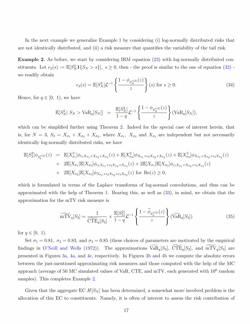
In the next example we generalize Example 1 by considering (i) log-normally distributed risks that
are not identically distributed, and (ii) a risk measure that quantifies the variability of the tail risk.
Example 2. As before, we start by considering IRM equation (23) with log-normally distributed con-
stituents. Let e2(s) := E[S2N1{SN > s}], s ≥ 0, then - the proof is similar to the one of equation (32) -
we readily obtain
e2(s) = E[S2N ]L−1
{1− φ
S∗(2)N
(z)
z
}(s) for s ≥ 0. (34)
Hence, for q ∈ [0, 1), we have
E[S2N | SN > VaRq[SN ]] =
E[S2N ]
1− qL−1
{1− φ
S∗(2)N
(z)
z
}(VaRq[SN ]),
which can be simplified further using Theorem 2. Indeed for the special case of interest herein, that
is, for N = 3, S3 = Xσ1 + Xσ2 + Xσ3 , where Xσ1 , Xσ2 and Xσ3 are independent but not necessarily
identically log-normally distributed risks, we have
E[S23 ]φ
S∗(2)3
(z) = E[X2σ1
]φc1Xσ1+Xσ2+Xσ3 (z) + E[X2σ2
]φXσ1+c2Xσ2+Xσ3 (z) + E[X2σ3
]φXσ1+Xσ2+c3Xσ3 (z)
+ 2E[Xσ1 ]E[Xσ2 ]φc1Xσ1+c2Xσ2+Xσ3 (z) + 2E[Xσ1 ]E[Xσ3 ]φc1Xσ1+Xσ2+c3Xσ3 (z)
+ 2E[Xσ2 ]E[Xσ3 ]φXσ1+c2Xσ2+c3Xσ3 (z) for Re(z) ≥ 0,
which is formulated in terms of the Laplace transforms of log-normal convolutions, and thus can be
approximated with the help of Theorem 1. Bearing this, as well as (33), in mind, we obtain that the
approximation for the mTV risk measure is
mTVq[S3] =1
CTEq[S3]× E[S2
3 ]
1− qL−1
1− φS∗(2)3
(z)
z
(VaRq[S3]) (35)
for q ∈ [0, 1).
Set σ1 = 0.81, σ2 = 0.83, and σ3 = 0.85 (these choices of parameters are motivated by the empirical
findings in O’Neill and Wells (1972)). The approximations VaRq[S3], CTEq[S3], and mTVq[S3] are
presented in Figures 3a, 4a, and 4e, respectively. In Figures 3b and 4b we compute the absolute errors
between the just-mentioned approximating risk measures and those computed with the help of the MC
approach (average of 50 MC simulated values of VaR, CTE, and mTV, each generated with 106 random
samples). This completes Example 2.
Given that the aggregate EC H[SN ] has been determined, a somewhat more involved problem is the
allocation of this EC to constituents. Namely, it is often of interest to assess the risk contribution of
17

0
5
10
15
20
25
30
35
40
45
50
0 0.2 0.4 0.6 0.8 1
(a)
0
0.0002
0.0004
0.0006
0.0008
0.001
0.0012
0.0014
0.0016
0 0.1 0.2 0.3 0.4 0.5 0.6 0.7 0.8 0.9 1
(b)
9
9.5
10
10.5
11
11.5
12
0.955 0.96 0.965 0.97 0.975 0.98 0.985 0.99
(c)
10
10.02
10.04
10.06
10.08
10.1
10.12
10.14
10.16
10.18
10.2
0.97 0.9705 0.971 0.9715 0.972
(d)
Figure 3: (a) Degree n = 20 approximation VaRq[S3], where σ1 = 0.81, σ2 = 0.83 and σ3 = 0.85. (b)
Absolute error between VaRq[S3] and the average of 50 MC simulations of VaRq[S3]. (c) VaRq[S3] (blue
line) compared to the maximum and minimum of VaRq[S3] computed using 50 MC simulations. (d) A
close-up of (c) at one point. All simulations are generated using 106 random samples.
18

6
8
10
12
14
16
18
20
0.75 0.8 0.85 0.9 0.95 1
(a)
0
0.002
0.004
0.006
0.008
0.01
0.012
0.014
0.016
0.018
0.02
0.022
0.75 0.8 0.85 0.9 0.95 1
(b)
16.5
17
17.5
18
18.5
19
19.5
20
20.5
21
0.991 0.992 0.993 0.994 0.995 0.996 0.997 0.998
(c)
18.6
18.8
19
19.2
19.4
0.995 0.9952 0.9954 0.9956 0.9958 0.996 0.9962 0.9964
(d)
8
10
12
14
16
18
20
0.75 0.8 0.85 0.9 0.95 1
(e)
Figure 4: (a) Degree n = 20 approximation CTEq[S3], where σ1 = 0.81, σ2 = 0.83 and σ3 = 0.85. (b)
Absolute error between CTEq[S3] and the average of 50 MC simulations of CTEq[S3]. (c) CTEq[S3] (blue
line) compared to the maximum and minimum of CTEq[S3] computed using 50 MC simulations. (d) A
close-up of (c) at one point. (e) Degree n = 20 approximation mTVq[S3] where σ1 = 0.81, σ2 = 0.83 and
σ3 = 0.85. All simulations are generated using 106 random samples.
19

each summand in (23) to H[SN ]. More formally, the allocation rule A : X × X → [0,∞] such that
A[X,X] = H[X] for X ∈ X assigns a finite (or infinite) value of the allocated EC to random pairs
(X,S) (e.g., Denault, 2001; Furman and Zitikis, 2008). One goal of the allocation exercise is profitability
testing, others are cost sharing and pricing (e.g., Venter, 2004).
Clearly, there are infinitely many ways to allocate the aggregate EC, and the literature on the allo-
cation rules is vast and growing rapidly (e.g., Dhaene et al., 2012, and references therein). In this paper
we work with the allocation counterparts of risk measures (24) and (25), which are, respectively,
CTEq[Xi, SN ] = E[Xi| SN > VaRq[SN ]], (36)
and
mTCoVq[Xi, SN ] := E[Xi| SN > VaRq[SN ]] +Cov[Xi, SN | SN > VaRq[SN ]
E[SN | SN > VaRq[SN ]], (37)
where i = 1, . . . , N , q ∈ [0, 1), and we assume that all the involved quantitites are well-defined and
finite. Obviously, we have CTEq[SN , SN ] = CTEq[SN ] and mTCoVq[SN , SN ] = mTVq[SN ] for i =
1, . . . , N, q ∈ [0, 1), and allocation rules (36) and (37) are fully additive. Moreover, these allocation
rules are ‘weighted’ (Furman and Zitikis, 2008), and they are therefore optimal in the sense of Dhaene
et al. (2012).
We are now ready to delve into the approximation of allocation rules (36) and (37).
Example 3. As in all previous examples, we consider a general IRM with log-normally distributed
standalone risks, and we specialize thereafter. Let h0(s) := E[Xj1{SN > s}], s ≥ 0, then - the proof is
at the end of this section,
h0(s) = E[Xj]L−1{
1
z
(1− φSN−Xj+X∗j (z)
)}(s) for s ≥ 0. (38)
This implies immediately, for q ∈ [0, 1) and cj = exp(σ2j ),
CTEq[Xj, SN ] =E[Xj]
1− qL−1
{1
z
(1− φ∑N
i=1, i6=j Xi+cjXj(z))}
(VaRq[SN ]).
Further, set N = 3, then
CTEq[Xj, S3] ≈E[Xj]
1− qL−1
{1
z
(1− φ∑3
i=1, i6=j Xi+cjXj(z))}
(VaRq[S3]) = CTEq[Xj, S3], , (39)
which is computed evoking Theorem 1.
In order to approximate the modified Tail Covariance allocation rule, we recall the following trivial
equation
Cov[Xj, SN | SN > VaRq[SN ]] = E[XjSN | SN > VaRq[SN ]]
− E[Xj| SN > VaRq[SN ]]× E[SN | SN > VaRq[SN ]] for q ∈ [0, 1).
20

The product of expectations can be computed as in Example 1, hence, we only need to approximate the
mixed expectation. To this end, let h(s) := E[XS1{S > s}], s ≥ 0, and note - the proof is at the end
of this section,
h(s) = E[Xj]E[SN,−j]L−1{
1
z
(1− φS∗N,−j+X∗j (z)
)}(s)
+ E[X2j ]L−1
{1
z
(1− φ
SN,−j+X∗(2)j
(z))}
(s),
where SN,−j :=∑N
i=1, i6=j Xi. This can be simplified with the help of Theorem 2, and in particular, for
N = 3, cj as before, and s ≥ 0,
h(s) = E[Xj]E[S3,−j]L−1{
1
z
(1−
3∑i=1, i6=j
E[Xi]
E[S3,−j]φcjXσj+ciXσi+
∑3k=1, k 6=i,j Xσk
(z)
)}(s)
+ E[X2j ]L−1
{1
z
(1− φS3,−j+c2jXj
(z))}
(s),
which implies, for cj = exp(σ2j ) and q ∈ [0, 1),
E[XjS3| S3 > VaRq[S3]] (40)
=E[Xj]E[S3,−j]
1− qL−1
{1
z
(1−
3∑i=1, i6=j
E[Xi]
E[S3,−j]φcjXσj+ciXσi+
∑3k=1, k 6=i,j Xσk
(z)
)}(VaRq[S3])
+E[X2
j ]
1− qL−1
{1
z
(1− φS3,−j+c2jXj
(z))}
(VaRq[S3])
≈ E[Xj]E[S3,−j]
1− qL−1
{1
z
(1−
3∑i=1, i6=j
E[Xi]
E[S3,−j]φcjXσj+ciXσi+
∑3k=1, k 6=i,j Xσk
(z)
)}(VaRq[S3])
+E[X2
j ]
1− qL−1
{1
z
(1− φS3,−j+c2jXj
(z))}
(VaRq[S3]),
which establishes the approximation of the conditional covariance, and can be computed using Theorem
1. Finally, the desired approximation of the modified Tail Covariance is
mTCovq[Xσi , S3] = CTEq[Xσi , S3] +Cov[Xj, S3| S3 > VaRq[S3]]
CTEq[S3], (41)
where CTEq[Xσi , S3] and CTEq[S3] are given in (39) and (33), respectively.
For visualization purposes, we again set σ1 = 0.81, σ2 = 0.83 and σ3 = 0.85, then the approximating
allocation rules based on the CTE and the modified Tail Covariance risk measures are depicted in Figures
5 and 6. This completes Example 3.
21

2
2.5
3
3.5
4
4.5
5
5.5
0.75 0.8 0.85 0.9 0.95 1
(a)
2
2.5
3
3.5
4
4.5
5
5.5
6
6.5
0.75 0.8 0.85 0.9 0.95 1
(b)
2.5
3
3.5
4
4.5
5
5.5
6
6.5
7
7.5
0.75 0.8 0.85 0.9 0.95 1
(c)
Figure 5: Degree n = 20 approximations (a) CTEq[X0.81, S3] (b) CTEq[X0.83, S3] and (c)
CTEq[X0.85, S3].
22

2.5
3
3.5
4
4.5
5
5.5
0.75 0.8 0.85 0.9 0.95 1
(a)
2.5
3
3.5
4
4.5
5
5.5
6
6.5
0.75 0.8 0.85 0.9 0.95 1
(b)
2.5
3
3.5
4
4.5
5
5.5
6
6.5
7
7.5
8
0.75 0.8 0.85 0.9 0.95 1
(c)
Figure 6: Degree n = 20 approximations (a) mTCovq[X0.81, S3] (b) mTCovq[X0.83, S3] (c)
mTCovq[X0.85, S3].
23

Proof of Equation (32). Note that the Laplace transform of e(s) is
L{e(s)}(z) =
∫ ∞0
e−zse(s)ds =
∫ ∞0
e−zs(∫ ∞
s
tf(t)dt
)ds =
1
z
∫ ∞0
(1− e−zt)tf(t)dt
=E[SN ]
z
∫ ∞0
(1− e−zt)dFS∗N (t) = E[SN ]
(1− φS∗N (z)
z
)for Re(z) ≥ 0. This completes the proof of the equation. ut
Proof of Equation (38). We have, for j = 1, . . . , N ,
L{h0(s)}(z) =
∫ ∞0
e−zsh0(s)ds =
∫ ∞0
e−zs∫ ∞0
∫ ∞s
ufXj ,SN (u, v)dvduds
=
∫ ∞0
e−zs∫ ∞0
ufXj(u)
(∫ ∞s−u
fSN−Xj(v)dv
)duds
= E[Xj]
∫ ∞0
e−zs∫ s
0
fX∗j (u)F SN−Xj(s− u)duds
= E[Xj]
∫ ∞0
e−zsF SN−Xj+X∗j (s)ds
for Re(z) ≥ 0. We then use property (ii) in Appendix A, which concludes the proof of the equation. ut
Proof of Equation 40. We have the following string of equations, for j = 1, . . . , N ,
L{h(s)}(z) =
∫ ∞0
e−zsh(s)ds =
∫ ∞0
e−zsE[XjSN1{S > s}]ds
=
∫ ∞0
e−zs∫ ∞0
∫ ∞s
uvfXj ,SN (u, v)dvduds
=
∫ ∞0
e−zs∫ ∞0
ufXj(u)
(∫ ∞s
vfSN−Xj(v − u)dv
)duds
= E[Xj]E[SN,−j]
∫ ∞0
e−zs∫ s
0
fX∗j (u)F S∗N,−j(s− u)duds
+ E[X2j ]
∫ ∞0
e−zs∫ s
0
fX∗(2)j
(u)F SN,−j(s− u)duds
= E[Xj]E[SN,−j]
∫ ∞0
e−zsF S∗N,−j+X∗j(s)ds+ E[X2
j ]
∫ ∞0
e−zsFSN,−j+X
∗(2)j
(s)ds
for Re(z) ≥ 0. This, along with property (ii) in Appendix A, completes the proof of the equation. ut
24

6 Aggregate economic capital determination: collective risk
model
In this section we assume that N is a discrete r.v., and so SN = Xσ1 + · · · + XσN is a collective risk
model with all of Xσ1 , Xσ2 , . . . independent mutually and on N , as well as identically distributed as a
canonical r.v. Xσ ∼ LN(σ2), σ > 0. Let GN(z) := E[zN ] denote the probability generating function
(p.g.f.) of N for all z ∈ (−∞, ∞) such that the p.g.f. is well-defined and finite.
In principle, once we have fixed the distributions of Xσ and N , we may proceed exactly as before and
approximate the Laplace transform of SN with the help of Theorem 1. This is clear from
φSN (z) = GN(φXσ(z)) ≈ GN(φXσ(z)) = φSN (z), Re(z) ≥ 0.
However, we must make a slight adjustment when computing the c.d.f FSN since the measure µ(dx) :=
P(SN ∈ dx) may have an atom at zero, and consequently FSN may be discontinuous there. We find that
better numerical results are achieved if we remove this atom.
More specifically, let µ({0}) = p0 ∈ (0, 1). The measure µ0(dx) := µ(dx) − p0δ0(dx) is absolutely
continuous with respect to the Lebesgue measure. It is easy to see that F0(x) := µ0([0, x]) has Laplace
transform φ0(z) := (φSN (z)− p0)/z, Re(z) ≥ 0. Therefore, we can use
FSN (x) = p0 + L−1 {φ0(z)} (x)
for the values of x near zero, and we revert to the methods in our preliminary examples otherwise.
Example 4. Let N be distributed Poisson with the unit rate parameter, and let SN = Xσ1 +Xσ2 + · · · ,where Xσ1 , Xσ2 , . . . are mutually independent, independent of N , and such that σ1 = σ2 = · · · = 0.83.
For this special N r.v., we have p0 = exp(−1). The graph of the approximation FSN (x) is shown in
Figure 7. Also shown therein is VaRq[SN ], which can be computed as the inverse of FSN (x) as before.
Of course in this case we have VaRq[SN] = 0 for q ≤ exp(−1). Using these results, we also compute
CTEq[SN ] and mTVq[SN ], which are depicted in Figure 8. This completes Example 4.
7 Computation time
In this section we provide the computation time needed to compute the quantities of interest in the
previous sections. These computation times are presented in Table 1.
All calculations were carried out on a desktop computer with 32GB of memory and an Intel i7-2600K
3.40GHz CPU. Times shown are measured in seconds. These represent the number of seconds required
25

0.3
0.4
0.5
0.6
0.7
0.8
0.9
1
0 5 10 15 20 25 30 35 40
(a)
0
5
10
15
20
25
30
35
40
0.3 0.4 0.5 0.6 0.7 0.8 0.9 1
(b)
Figure 7: Degree n = 20 approximations (a) FSN (x) and (b) VaRq[SN ].
4
6
8
10
12
14
16
0.75 0.8 0.85 0.9 0.95 1
(a)
4
6
8
10
12
14
16
18
0.75 0.8 0.85 0.9 0.95 1
(b)
Figure 8: Degree n = 20 approximations (a) CTEq[SN ] and (b) mTVq[SN ].
26
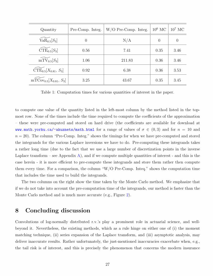
Quantity Pre-Comp. Integ. W/O Pre-Comp. Integ. 106 MC 107 MC
VaR0.5[S3] 0 N/A 0 0
CTE0.5[S3] 0.56 7.41 0.35 3.46
mTV0.5[S3] 1.06 211.83 0.36 3.46
CTE0.5[X0.81, S3] 0.92 6.38 0.36 3.53
˜mTCov0.5[X0.81, S3] 3.25 43.67 0.35 3.45
Table 1: Computation times for various quantities of interest in the paper.
to compute one value of the quantity listed in the left-most column by the method listed in the top-
most row. None of the times include the time required to compute the coefficients of the approximation
– these were pre-computed and stored on hard drive (the coefficients are available for download at
www.math.yorku.ca/~akuznets/math.html for a range of values of σ ∈ (0, 3) and for n = 10 and
n = 20). The column “Pre-Comp. Integ.” shows the timings for when we have pre-computed and stored
the integrands for the various Laplace inversions we have to do. Pre-computing these integrands takes
a rather long time (due to the fact that we use a large number of discretization points in the inverse
Laplace transform – see Appendix A), and if we compute multiple quantities of interest - and this is the
case herein - it is more efficient to pre-compute these integrands and store them rather then compute
them every time. For a comparison, the column “W/O Pre-Comp. Inteq.” shows the computation time
that includes the time used to build the integrands.
The two columns on the right show the time taken by the Monte Carlo method. We emphasize that
if we do not take into account the pre-computation time of the integrands, our method is faster than the
Monte Carlo method and is much more accurate (e.g., Figure 2).
8 Concluding discussion
Convolutions of log-normally distributed r.v.’s play a prominent role in actuarial science, and well-
beyond it. Nevertheless, the existing methods, which as a rule hinge on either one of (i) the moment
matching technique, (ii) series expansion of the Laplace transform, and (iii) asymptotic analysis, may
deliver inaccurate results. Rather unfortunately, the just-mentioned inaccuracies exacerbate when, e.g.,
the tail risk is of interest, and this is precisely the phenomenon that concerns the modern insurance
27

regulation the most. In this paper we have proposed a hybrid approach to resolving the problem. More
specifically, we have shown that it is possible to approximate the distribution of the sum of independent
and log-normally distributed r.v.’s with the help of the distribution of n-fold gamma convolutions in
such a way that the two are arbitrarily close. We then have utilized the class of Pade approximations
to find the parameters of the approximating distribution. For the convenience of the end-user, we have
pre-computed these parameters for a range of values of σ ∈ (0, 3) and for n = 10 and n = 20: these can
be downloaded at www.math.yorku.ca/~akuznets/math.html.
Remarkably, the algorithm that arises from our method is fast, accurate, and, last but not least, very
versatile. We have discussed the two former advantages earlier in the paper, and so we touch on the
versatility in more detail here. In this respect, recall that the thrust of our method is the observation that
the log-normal distribution is a member of the encompassing class of the generalized gamma convolutions.
Indeed this is how the link to the finite gamma convolutions emerges. Another distribution that belongs
to the class of generalized gamma convolutions - and is popular in actuarial science - is Pareto (e.g.,
Bondesson, 1992).
Consider the following p.d.f. of a Pareto distributed r.v. Y with shape parameter α > 0
f(y) = α(1 + y)−α−1, y > 0. (42)
Pareto is a classical example of a heavy-tailed distribution, and it holds that for the values α ∈ (1, 2]
the variance of Y is infinite, and for the values α ∈ (0, 1] even the mean of Y is infinite. We now quickly
apply our method to illustrate how it can be used in order to approximate p.d.f. (42), as well as the
corresponding c.d.f. We note in passing that the approximating c.d.f. of the sum of independent but not
necesserily identically Pareto-distributed r.v.’s can be computed along the line of Corollary 1 (see, e.g.,
Ramsay, 2009, that considers the situation of i.i.d. summands). In Seal (1980), it is mentioned that in
the real-world applications (e.g., fire and auto-mobile losses, to name a few), insurers have to frequently
deal with Pareto-distributed risks with infinite variances and finite means. Therefore in our illustration
below we choose α = 1.5.
We set z∗ = 1, run the approximation algorithm from Section 3 for n = {2, 4, 6, 8, 10, 20, 30, 40}in order to find the approximating Laplace transform, and then use the inversion method from Appendix
A to find the p.d.f. We compute the approximating c.d.f. over 200 points equally spaced over the
interval [0, 20], and compare the result with the exact one that follows from formula (42). The outcomes
are depicted in Figure 9. Noticeably, even lower orders of approximations, provide practically visually
indistinguishable results.
28

0 5 10 15 200
0.1
0.2
0.3
0.4
0.5
0.6
0.7
0.8
0.9
1
(a)
0 5 10 15 20 2510 -8
10 -7
10 -6
10 -5
10 -4
10 -3
(b)
Figure 9: (a) The black curve is the exact Pareto c.d.f. (with α = 1.5), the green (respectively, blue)
curve is the c.d.f. of the approximations Y2 (respectively, Y4). (b) The difference between the Pareto
c.d.f. and the c.d.f. of Yn for n ∈ {10, 20, 30, 40} (larger values of n correspond to smaller errors).
Acknowledgements
We are grateful to the Casualty Actuarial Society award under the umbrella of the 2017 Individual
Grants Competition for the support that has enabled us to concentrate our time and energy on this
project. Edward Furman and Alexey Kuznetsov also acknowledge the continuous financial support of
their research by the Natural Sciences and Engineering Research Council of Canada. Daniel Hackmann
was supported by the Austrian Science Fund (FWF) under the project F5508-N26, which is part of the
Special Research Program “Quasi-Monte Carlo Methods: Theory and Applications”.
9 References
Allen, G. D., Chui, C. K., Madych, W. R., Narcowich, F. J., and Smith, P. W. (1975). Pade approximation
of Stieltjes series. Journal of Approximation Theory, 14:302–316.
Artzner, P., Delbaen, F., Eber, J.-M., and Heath, D. (1999). Coherent measures of risk. Mathematical
Finance, 9(3):203–228.
Asmussen, S., Jensen, J. L., and Rojas-Nandayapa, L. (2011). A literature review on log-normal sums.
Technical report, University of Queensland.
29

Asmussen, S. and Rojas-Nandayapa, L. (2008). Asymptotics of sums of lognormal random variables with
Gaussian copula. Statistics and Probability Letters, 78(16):2709–2714.
Baker, G. A. and Graves-Morris, P. (1996). Pade Approximants. Cambridge University Press, Cambridge-
New-York, second edition.
Beaulieu, N. C., McLane, P. J., and Abu-Dayya, A. A. (1995). Estimating the distribution of a sum of
independent lognormal random variables. IEEE Transactions on Communications, 43(12):2869–2873.
Bickerstaff, D. R. (1972). Automobile collision deductibles and repair cost groups: the log-normal model.
Proceedings of the Casualty Actuarial Society, LIX:68.
Bondesson, L. (1992). Generalized Gamma Convolutions and Related Classes of Distributions and Den-
sities. Springer-Verlag, New-York, lecture notes in statistics edition.
Bondesson, L. (2002). On the Levy measure of the lognormal and the logcauchy distributions. Method-
ology and Computing in Applied Probability, (4):243 – 256.
Chen, S., Nie, H., and Ayers-Glassey, B. (2008). Lognormal sum approximation with a variant of Type
IV Pearson distribution. IEEE Communications Letters, 12(9):630–632.
Denault, M. (2001). Coherent allocation of risk capital. Journal of risk, (514):1–34.
Denuit, M., Dhaene, J., Goovaerts, M., and Kaas, R. (2006). Actuarial Theory for Dependent Risks:
Measures, Orders and Models. John Wiley & Sons, The Atrium, Southern Gate, Chichester.
Denuit, M., Dhaene, J., and Ribas, C. (2001). Does positive dependence between individual risks increase
stop-loss premiums? Insurance: Mathematics and Economics, 28(3):305–308.
Dhaene, J., Henrard, L., Landsman, Z., Vandendorpe, A., and Vanduffel, S. (2008). Some results on the
CTE-based capital allocation rule. Insurance: Mathematics and Economics, 42(2):855–863.
Dhaene, J., Tsanakas, A., Valdez, E. A., and Vanduffel, S. (2012). Optimal capital allocation principles.
Journal of Risk and Insurance, 79(1):1–28.
Dropkin, L. B. (1964). Size of loss distributions in workmens compensation insurance. Proceedings of
the Casualty Actuarial Society, LI:198.
Dufresne, D. (2008). Sums of log-normals. In Actuarial Research Conference Proceedings.
EIOPA-14-322 (2014). The underlying assumptions in the standard formula for the Solvency Capital
Requirement calculation. Technical report, European Insurance and Occupational Pensions Authority.
30

Fenton, L. F. (1960). The sum of log-normal probability distributions in scatter transmission systems.
IRE Transactions on Communications Systems, 8(1):57–67.
Filon, L. N. (1928). On a quadrature formula for trigonometric integrals. Proceedings of the Royal Society
of Edinburgh, 49:38–47.
Fosdick, L. D. (1968). A special case of the Filon quadrature formula. Mathematics of Computation,
22:77–81.
Furman, E. and Landsman, Z. (2005). Risk capital decomposition for a multivariate dependent gamma
portfolio. Insurance: Mathematics and Economics, 37(3):635–649.
Furman, E. and Landsman, Z. (2006). Tail variance premium with applications for elliptical portfolio of
risks. ASTIN Bulletin: The Journal of the International Actuarial Association, 36(2):433–462.
Furman, E. and Zitikis, R. (2008). Weighted risk capital allocations. Insurance: Mathematics and
Economics, 43(2):263–269.
Holgate, P. (1989). The log-normal characteristic function. Communications in Statistics - Theory and
Methods, 18(12):4539–4548.
Hurlimann, W. (2003). Conditional Value-at-Risk bounds for compound Poison risks and a normal
approximation. Journal of Applied Mathematics, 3:141–153.
Jiang, C.-F., Peng, H.-Y., and Yang, Y.-K. (2016). Tail variance of portfolio under generalized Laplace
distribution. Applied Mathematics and Computation, 282:187–203.
Kaas, R., Goovaerts, M., Dhaene, J., and Denuit, M. (2008). Modern Actuarial Risk Theory Using R.
Springer-Verlag, Berlin, Heidelberg, second edition.
Kleiber, C. and Kotz, S. (2003). Statistical Size Distributions in Economics and Actuarial Sciences.
Wiley & Sons, Hoboken, New Jersy.
Klugman, S. A., Panjer, H. H., and Willmot, G. E. (2012). Loss Models: From Data to Decisions. Wiley
& Sons, Hoboken, New Jersy, third edition.
Leipnik, R. B. (1991). On log-normal random variables: 1 - the characteristic function. Journal of
Australian Mathematical Society Series B, 32:327–347.
Limpert, E., Stahel, W. A., and Abbt, M. (2001). Log-normal distributions across the sciences: Keys
and clues. BioScience, 51(5):341–352.
31

McNeil, A. J., Frey, R., and Embrechts, P. (2005). Quantitative Risk Management: Concepts, Techniques
and Tools. Princeton University Press, New-York.
Mikosch, T. (2009). Non-Life Insurance Mathematics: An Introduction with Poisson Process. Springer-
Verlag, Berlin, Heidelberg.
Milevsky, M. A. and Posner, S. E. (1998). Asian options, the sum of lognormals, and the reciprocal
gamma distribution. Journal of Financial & Quantitative Analysis, 33(3):409–421.
O’Neill, B. and Wells, W. T. (1972). Some recent results in lognormal parameter estimation using
grouped and ungrouped data. Journal of the American Statistical Association, 67(337):76–80.
Patil, G. P. and Rao, C. R. (1978). Weighted distributions and size-biased sampling with applications
to wildlife populations and human families. Biometrics, 34(2):179–189.
Ramsay, C. M. (2009). The distribution of compound sums of Pareto distributed losses. Scandinavian
Actuarial Journal, 2009(September 2014):27–37.
Seal, H. L. (1980). Survival probabilities based on Pareto claim distributions. ASTIN Bulletin: The
Journal of the International Actuarial Association, (11):61 – 74.
Sprenkle, C. M. (1964). Warrant prices as indicator of expectation. Yale Economic Essays, 1:412–474.
Takahasi, H. and Mori, M. (1974). Double exponential formulas for numerical integration. Publ. RIMS
Kyoto Univ, 9:721–741.
Thorin, O. (1977). On the infinite divisibility of the lognormal distribution. Scandinavian Actuarial
Journal, 1977(3):121–148.
Vanduffel, S., Chen, X., Dhaene, J., Goovaerts, M., Henrard, L., and Kaas, R. (2008). Optimal ap-
proximations for risk measures of sums of lognormals based on conditional expectations. Journal of
Computational and Applied Mathematics, 221(1):202–218.
Venter, G. G. (2004). Capital allocation survey with commentary. North American Actuarial Journal,
8(2):96 – 107.
Wang, S. S. (1996). Premium calculation by transforming the layer premium density. ASTIN Bulletin:
the Journal of the International Actuarial Association, 26(26):71 – 92.
Zhang, K. Q. T. and Song, S. H. (2008). A systematic procedure for accurately approximating lognormal-
sum distributions. IEEE Transactions on Vehicular Technology, 57(1):663–666.
32

Appendix A Numerical inversion of Laplace transform
In this section we remind the reader some results from the theory of Laplace transform and discuss how
to compute the inverse Laplace transform efficiently and accurately. Let f be a p.d.f. and define by φ
the corresponding Laplace transform
φ(z) = Lf(z) =
∫ ∞0
e−zxf(x)dx, Re(z) ≥ 0.
The following results are well-known:
(i) If f is sufficiently smooth, then
f(x) = L−1{φ(z)}(x) =1
2πi
∫ c+i∞
c−i∞ezxφ(z)dz, (43)
where c is an arbitrary positive number.
(ii) Let F be the c.d.f. corresponding to f and F := 1 − F . Then LF (z) = φ(z)/z and LF (z) =
(1− φ(z))/z.
Let us now discuss how to compute the inverse Laplace transform efficiently. Assume that the function
φ is analytic in C\ (−∞, 0] and it converges to zero uniformly as z →∞ in this domain. Note that these
conditions, while rather restrictive in general, are always satisfied in examples used in the present paper
(see formula (8), for example). We begin by writing the inverse Laplace transform in an equivalent form
f(x) = Im
(1
π
∫ c+i∞
c
ezxφ(z)dz
), x ≥ 0, (44)
which follows from the fact φ(z) = φ(z). Now we choose a in the second quadrant (that is, arg(a) ∈(π/2, π)), rotate the contour of integration and change the variable of integration z = c+ au and obtain
the following integral representation
f(x) = Im
(aecx
π
∫ ∞0
euRe(a)xeiu Im(a)xφ(c+ au)du
), x ≥ 0. (45)
The above integral is more convenient to work with, compared to (44), for the following reason: the
integrand decays exponentially fast in (45) as Re(a) < 0 .
In the computations in Sections 4, 5 and 6, we typically choose −0.5 ≤ Re(a) ≤ −0.1, Im(a) = 1
and 0.25 ≤ c ≤ 5. To compute the oscillatory integral (45), we use the Filon’s quadrature (Filon, 1928;
Fosdick, 1968). This entails approximating φ(c+ au) locally by a polynomial of degree two (using three
discretization points), and integrating the result against the exponential function. In total, we typically
truncate the integral in (45) at a point in the interval [250, 500] and use between 500,001 and 1,000,001
unevenly spaced discretization points to evaluate the resulting integral.
33