on-line hplc phase-modulation
TRANSCRIPT

ON-LINE HPLC / PHASE-MODULATION
FLUORESCENCE LIFETIME
DETERMINATIONS FOR
POLYCYCLIC AROMATIC
HYDROCARBONS
By
WILLIAM TYLER COBB
Bachelor of Science in Chemistry
Southeastern Oklahoma State University
Durant, Oklahoma
1984
Submitted to the Faculty of the Oklahoma State University in partial fulfillment of
the requirements for the Degree of
DOCTOR OF PHILOSOPHY December, 1989

DEDICATION
Dedicated to My Wife,
Irma
and Children,
Carolina, Steven and Salvador
1360153

ON-LINE HPLC / PHASE-MODULATION
FLUORESCENCE LIFETIME
DETERMINATIONS FOR
POLYCYCLIC AROMATIC
HYDROCARBONS
Thesis approved:
Dean of the Graduate College
ii

PREFACE
This dissertation describes efforts to incorporate on
line fluorescence lifetime selectivity into the detection
and determination of polycyclic aromatic hydrocarbons
separated by high performance liquid chromatography. This
goal was approached through the use of multifrequency
phase-modulation fluorescence spectroscopy and non-linear
least squares fluorescence lifetime heterogeneity analysis.
The technique yields phase and modulation fluorescence
lifetimes at several points along each chromatographic
peak; peak heterogeneity is indicated if present, and
components in unresolved peaks can be quantitated without
the need for chromatographic resolution.
The support of several agencies and institutions was
critical to the eventual completion of this work and I wish
to acknowledge and extend my sincere thanks to them. First
I want to thank the United States Environmental Protection
Agency which was gracious enough to fund this project
through its entirety. Special thanks goes to the OSU
Center for Water Research which supplied funding for the
purchase of an HPLC, and also for a very nice and
appreciated Presidential Fellowship while I was at OSU. My
appreciation is extended to Oklahoma State University for
providing support in the form of teaching assistantships
iii

and scholarships. Lastly, I would like to thank Duke
University and the people in the Duke chemistry department
who very much helped make the transition from Oklahoma a
much smoother and enjoyable experience than it otherwise
would have been.
I would like to express my sincere gratitude to
several individuals without whose help, encouragement, and
understanding I would never have made it this far. My
research advisor, Dr. Linda B. McGown, in addition to being
an unending source of research-related ideas and
encouragement, was equally supportive and understanding of
issues outside of the laboratory. Without this
understanding, attempting to simultaneously raise a family
and pursue a Ph.D. in chemistry would surely have resulted
in failure in either one or both of these areas. I would
also like to thank the McGown research group for putting up
with me through thick and thin and especially to Kasem
Nithipatikom and Dave Millican for their support,
friendship and extensive help during my graduate career.
A special note of appreciation goes to my parents and
sisters whose expressions of joy and encouragement during
each phase of my educational career have provided me with
unequalled inspiration and hope to reach each subsequent
step in the climb to where I am now.
Above all my deepest and most heartfelt thanks goes to
my wife, Irma, who has been a source of undying support and
inspiration in spite of all the hardships, both financial
iv

and emotional, that pursuing a Ph.D. has placed on our
marriage and on our family. She unfortunately was forced
to delay her graduate studies in order to raise and support
our children, and now it's her turn to finish up her Ed.D.
in Adapted Physical Education. I would also like to thank
my wife and children for being my critical link to the real
world outside of graduate school, and it is to them that I
dedicate this dissertation.
v

TABLE OF CONTENTS
Chapter Page
I. INTRODUCTION. 1
II. DETERMINATION OF POLYCYCLIC AROMATIC HYDROCARBONS ........... . 5
Separation Techniques. . . . . . . . . 5 Detection And Peak Purity Determination
For HPLC . . . . . . . . . . . . . . . . 21
III. FLUORESCENCE LIFETIME THEORY AND APPLICATIONS . 49
IV.
v.
Fluorescence: A General Description. . 49 Fluorescence Lifetime Theory . . . . . 52 Heterogeneity Analysis Based On Phase-
Modulation Lifetimes . . . · . . . . . 63 On-line Fluorescence Lifetime Detection
For HPLC . . . . . . . . . . . . 77
EXPERIMENTAL ...
Chemicals ..... . Instrumentation.
RESULTS AND DISCUSSION ....
87
87 88
104
Characterization Of Test Compounds . . . . 104 On-Line Fluorescence Lifetime
Determinations . . . . . . . . . . . . . 111 Application of Phase-Modulation
Fluorescence Lif~time Determinations and Heterogeneity Analysis To Mixtures of B(k)F and B(b)F. . . . . . . . . . . . . 124
Fluorescence Lifetimes for PAHs On-line With HPLC Using A Multifrequency PhaseModulation Fluorometer. . . . . . . . . 134
Fluorescence Lifetimes, Heterogeneity Detection, and Heterogeneity Analysis for Mixtures of PAHs Using HPLC and Multifrequency Phase-Modulation Fluorescence . . . . . . . . . . . . . . 162
vi

Chapter
VI.
Phase-Modulation Fluorescence Lifetime Chromatograms and Heterogeneity Analysis for the Sixteen EPA Priority Pollutant
Page
PAHs . . . . . . . . . . . . . . . . . . 169 Related Studies: On-Line HPLC/Phase
Resolved Fluorescence Intensity (PRFI) Detection of PAHs. . . . . . . . . . 184
CONCLUSION. 194
BIBLIOGRAPHY . 197
APPENDICES . .
APPENDIX A - COMPUTER PROGRAM WRITTEN IN MICROSOFT QUICKBASIC TO CALCULATE INTENSITY-MATCHED LIFETIMES FOR
202
CHROMATOGRAMS . . . . . . . . 203
APPENDIX B - COMPUTER PROGRAM WRITTEN IN MICROSOFT QUICKBASIC TO CALCULATE FRACTIONAL INTENSITIES FROM FRACTIONAL CONTRIBUTIONS OBTAINED FROM HETEROGENEITY ANALYSES. . . . 209
vii

LIST OF TABLES
Table Page
1. EPA Priority Pollutant PAR 2
2. Identification of PARs for Figures 1 and 2 . 13
3. Values of k' for PARs Using LiChrosorb RP-18 . . 18
4. Minimum Detectable Quantities Using UV Absorbance and Fluorescence Detection
5. Detection Limits Using a Diode-Array Absorbance
34
Detector.............. . ... 40
6. Fluorescence Lifetimes of Tryptophan at Different pH Values . . . . . . . . . . . .
7. Resolved Lifetimes for Data in Table 6 Using Weber's Algorithm . . . .
8. Resolved Lifetimes for 1:3 Mixture of Perylene and 9-Arninoacridine Using NLLS With 5, 10, 20,
66
. 66
40 and 80 MHZ . . . . . . . . . . . . . . . . . 71
9. Computer Program Routines. 74
10. Resolved Fluorescence Lifetimes of Pyrene and Carbazole. . . . . . . . . . . . . . . . . 7 5
11. Resolved Fluorescence Lifetime of POPOP in the Presence of Pyrene and Carbazole . . . . . . . 76
12. Fluorescence Excitation and Emission Maxima. 106
13. Phase and Modulation Fluorescence Lifetimes. 108
14. Fluorescence Lifetimes for B(k)F 117
15. Fluorescence Lifetimes for B(k)F Along a Peak. . 119
16. Results for Batch Heterogeneity Analysis for B(k)F and B(b)F. . . . . . . . . . . . 128
17. Relative Errors for On-Line Heterogeneity Analysis . . . . . . . . . . . . . . . . 132
viii

Table Page
18. Mixtures of B(b)F and B(k)F for Heterogeneity Analysis . . . . . . . . . . . . . . . . . . . 138
19. Fluorescence Lifetimes of Mixtures of B(b)F and B(k)F ..................... 139
20. Results of Batch NLLS Heterogeneity Analysis 140
21. List of PAHs Used in Analysis in Order of HPLC Elution. . . . . . . . . . . . . . . . 172
22. Peak Identification for Figures 78 and 79. 189
ix

LIST OF FIGURES
Figure
1. Separation of PARs Using Isocratic Elution With 80% Aqueous MeCN. . ..... .
2. (a) Separation of PARs Using Gradient Elution. (b) Solvent Program for (a) Using Aqueous
Page
11
MeCN . . . . . . . . . . . . . . . . . . . 12
3. Separation of PARs Using EPA Method 610. . . 16
4. Isothermal Separation of PARs Using 80% Aqueous MeCN . . . . . . . . . . . . . . . . . . . 19
5. Temperature Gradient Separation of PARs Using 80% Aqueous MeCN . . . . . . . . . . . . . . . 20
6. LC/MS Separation of Phenanthrene, 9-Methylanthracene, and Fluoranthene
7. Comparison of Direct Deposition and Spray Deposition of HPLC Eluent With Moving Belt
25
Interface for LC/MS. . . . . . . . . . . . 26
8. Comparison of UV and MS Detection for Normal Phase LC . . . . . . . . . . . . . . . 27
9. Comparison of UV and MS Detection for Reversed-Phase LC . . . . . . . . . . . . . . . 2 8
10. Simultaneous UV Diode-Array and MS Detection. Inserts Show UV Absorbance and Mass Spectra of Benzo(a)pyrene . . . . . . . . . . . . . . 30
11. UV Absorbance Detection Using 3 Detectors in Series . . . . . . . . . . . . . . . . . . . . 33
12. UV Absorbance and Fluorescence Detection. (A)
13.
PAH Standards, (B) Alkylated Naphthalenes, (C) Refinery Effluent After Enrichment . . . . . . 35
Effects. of Baseline Drift and Offsets on Absorbance Ratios .......... . 37
X

Figure
14. Practical Effects of Peak Overlap and Peak Tailing on Absorbance Ratios . . . . . .
15. Separation of (1) Pyrene, (2) Fluoranthene, (3) Benzo(e)pyrene, (4) Biphenyl, (5) Fluorene, (6) Phenanthrene, (7) Naphthalene, (8)
Page
37
Acenaphthylene . . . . . . . . . . . . . . 45
16. Fluorescence Chromatogram of (a) Anthracene, (b) Chrysene, and (c) Benzo(a)pyrene . . . 47
17. Constant Energy Synchronous Luminescence Spectra of the Three Peaks in Figure 16. . 47
18. Exponential Fluorescence Decay After Pulsed Excitation . . . . . . . . . . . . . . 54
19. Least-Squares Reconvolution of a Two-Component Decay Using Single and Double Exponential Decay Laws for Fitting . . . . . . . . . . 55
·20. Component Stripping for Two-Component Decay. 57
21. Excitation (E(t)) and Emission (F(t)) Functions for Harmonic Excitation Showing the Demodulation m and Phase Shift q,· • • • • • • • 59
22. Divergence of Calculated Lifetimes From an Arithmetic Mean of 4 ns in Heterogeneous Systems of Two Components of Equal Intensity . 61
23. Divergence of Lifetimes in Two-Component Systems of 1 and 8 ns and Different Relative Intensity (weight) . . . . . . . . . . . . . . . . . . . 62
24. Relative Fluorescence Intensity and Fluorescence Lifetimes as a Function of pH for Tryptophan . 65
25. Distribution of Resolved Lifetimes Using Weber's Algorithm With More Than Two Frequencies for a Two-Component System of 3.1 and 8.7 ns . . . . 67
26. Phase and Modulation as a Function of Modulation Frequency for a Two-Component System of 3.1 and 8 • 7 ns . . . . . . . . . . . . . . . . . . 6 9
27. Errors in Resolved Lifetimes Using Weber's Algorithm as a Function of Frequency With One Frequency Fixed at 30 MHz. . . . . . . . . . . 70
28. Uncertainty in the Resolved Components of the 3.1 and 8.7 ns System Using NLLS . . . . . . . . . 71
xi

Figure Page
29. Resolved Lifetimes for Anthracene (4 ns) and 9-CNA (12 ns) Using Global, Conventional, and Algebraic (Weber's) Heterogeneity Analyses . . 78
30. Resolved Lifetimes for System in Figure 29 With Dynamic Quencher Added to Yield Lifetimes of 3.9 and 7.2 ns for Anthracene and 9-CNA. . . . 79
31. Fluorescence Detection of Six PAHs Using Pulsed Excitation and Time Delays of (a) 0 ns, (b) 15 ns, and (c) 45 ns. . . . . . . . . . . . . 81
32. Fluorescence Detection of B(a)P and B(ghi)P Using Pulsed Excitation and Time Delays of (A) 0 ns and (B) 20 ns . . . . . . . . . . 81
33. Instrumental Setup to Obtain 10 ns Delay Between Oscilloscope Inputs. . . . . . . . 83
34. Position of Oscilloscope Apertures for Ratio Measurement. . . . . . . . . . . . . . 83
35. Illustration of the Two Channels of Raw Data (a,b) and Their Ratio (c) for Fluoranthene 84
36. Two-Component Peak Consisting of Perylene and Benzo(a)pyrene Showing How the Ratiogram Can Resolve Overlapping Peaks. . . . . . . . . . . 85
37. General Diagram of HPLC/UV/Spectrofluorometer Setup. . . . . . . . . . . . . . . . . . . . . 89
38. SLM 4800S Phase-Modulation Spectrofluorometer. . 92
39.
40.
Debye-Sears Modulation Tank for SLM 4800S.
SLM 48000S Multifrequency Phase-Modulation Spectrofluorometer . . . . . . . . . . .
41. Beam Path Through Modulation Compartment for Dynamic Measurements Showing Q-Switch
95
96
Polarizer (Q) and Peckel's Cell (P). . 98
42. Beam Path Through Modulation Compartment for Steady-State Measurements Showing Mirror (M) 99
43. Chromatogram of 11 PAHs Using Gradient Elution and UV Absorbance Detection at 254 nm. . . . . 109
44. Fluorescence Lifetimes vs. HPLC Retention Time Time for PAHs From Figure 43 . . . . . . . . . 110
xii

Figure Page
45. Lifetime vs. Percent Aqueous Acetonitrile as Solvent. . . . . . . . . . . . . . . . 113
46. Lifetimes vs. Time Using Scatter as the Reference. . . . . . . . . . . . . . . . . . .
47. Lifetimes vs. Time Using DimethylPOPOP as the Reference. . . . . . . . . . . . . . . . . . .
48. Chromatograms of B(k)F and B(b)F Using Different Mobile Phase Compositions With Isocratic
122
123
Elution. . . . . . . . . . . . . . . . 130
49. Fluorescence Lifetime Chromatogram for B(k)F at 0.5 mL/min and 100% MeCN . . . . . . .
50. Fluorescence Lifetime Chromatograms of B(k)F Using 100% MeCN at (a) 0.2 and (b) 0.4 mL/min.
51. Fluorescence Lifetime Chromatograms of B(k)F Using 100% MeCN at (a) 0.6 and (b) 0.8 mL/min.
52. Fluorescence Lifetime Chromatograms at 0.5 mL/min and 80% MeCn for (a) B(k)F and (b)
142
144
145
B(b)F. . . . . . . . . . . . . . . . . . . 147
53. Fluorescence Lifetime Chromatograms at 0.5 mL/min and 90% Aqueous MeCN for (a) B(k)F and (b) B(b)F. . . . . . . . . . . . . . . . . 148
54. Fluorescence Lifetime Chromatograms at 0.5 mL/min and 100% MeCN for (a) B(k)F and (b) B(b)F. . . . . . . . . . . . . . . . . 149
55. Batch Fluorescence Lifetime Chromatogram Simulations for B(k)F (a) Before and (b) After Reference Intensity Matching . . . . . . . . . 150
56. Stopped-Flow Fluorescence Lifetime Chromatogram Simulations for B(k)F (a) Before and (b) After Reference Intensity Matching . . . . . . . 152
57. Dynamic (a.c.) and Steady-State (d.c.) Intensities and Modulation (a.c./d.c.) vs. Time for B(k)F . . . . . . . . . . . . 154
58. Fluorescence Lifetime Chromatograms for Fluoranthene at 0.3 mL/min and 100% MeCN Before and (b) After Reference Intensity Matching and a.c. Correction ..... .
xiii
(a)
156

Figure
59. Fluorescence Lifetime Chromatograms for B(k)F With 100% MeCN at (a) 0.3, (b) 0.5, (c) 0.8,
Page
and (d) 1.0 mL/min . . . . . . . . . . . . . . 158
60. Fluorescence Lifetime Chromatograms for B(k)F at 0.5 mL/min With (a) 70%, (b) 80%, (c) 90%, and (d) 100% MeCN ................. 160
61. Fluorescence Lifetime Chromatogram Using 10 MHz Modulation Frequency, 100% MeCN, and 0.3 mL/min . . . . . . . . . . . . . . . . . . . . 164
62. NLLS Heterogeneity Analysis Results for Fractional Contributions Using 4, 10, 15, 25, and 35 MHz . . . . . . . . . . . . . . . . . . 166
63. NLLS Heterogeneity Analysis Results for Fractional Contributions With Lifetimes Fixed Using the Same Frequencies as in Figure 62 168
64. Intensity Output and Modulation of 450 Watt Xenon Arc Lamp vs. Wavelength ..... .
65. Chromatograms of Compounds Listed in Table 21 Using 0.5 mL/min, 80% Aqueous MeCN and Fluorescence Detection With (a) Ex=330 nm, Em=345 nm LP + 600 nm SP Filters, (b)
171
Ex=360 nm, Em=399 nm LP + 600 nm SP Filters .. 173
66. Excitation and Emission Spectra of Black Quartz Fluorescence Flow Cell . . . . . . . . . . 175
67. Effect of Flow Cell Luminescence on Lifetime Chromatograms of B(k)F . . . . . . . . 177
68. Chromatogram of 11 Compounds Using 0.3 mL/min and 8 7% Aqueous MeCN . . . . . . . . . 17 9
69. Lifetime Chromatogram for 11 Compounds at 10 MHz Modulation Frequency . . . . . . . . . . . . . 180
70. Data From Figure 69 Expanded in Time .
71. (a) Heterogeneity Analysis Results Using NLLS and Frequencies of 5, 10, 15, 25, and 40 MHz.
181
(b) Same as in (a) but With Lifetimes Fixed. . 183
72. PRFI Resulting From Setting the Detector Phase (a) Exactly in Phase With a.c. Curve, (b) Exactly Out of Phase With a.c., and (c) at an Arbitrary Location on the a.c. Curve . . . 186
xiv

Figure Page
73. PRFI Chromatograms vs. Frequency With Detector Phase Set to Null Out Scattered Light. . . . . 191
74. PRFI Chromatograms at 10 MHz With Detector Phase Set to Null Out (a) Scattered Light, (b) 7 ns Contribution, and (c) 25 ns Contribution . . . 192
XV

CHAPTER I
INTRODUCTION
One of the largest classes of environmental pollutants
known today is the polycyclic aromatic hydrocarbons (PAHs),
which are the homologs of benzene in which three or more
aromatic rings are joined in various configurations. These
compounds are important due to their carcinogenic,
precarcinogenic, and/or mutagenic characteristics (1,2,3).
The environmental concern about PAHs led the World Health
Organization (WHO) to recommend that the total
concentration of six specific PAHs not exceed 200 ng/L for
domestic drinking water (4) . The six specified PAHs are
listed in Table 1 and designated by the asterisks. The
Environmental Protection Agency (EPA) also designates
sixteen EPA Priority Pollutant PAHs which are also shown in
Table 1 along with their molecular weights, structures, and
carcinogenic potentials (5) .
Polycyclic aromatic hydrocarbons can be formed from
both natural and anthropogenic sources; however, the latter
have been by far the major contributors in the past several
decades. Natural sources include volcanos, forest fires,
biosynthesis, and long-term degradation followed by
synthesis from biological material. Anthropogenic sources
1

2
TABLE 1
EPA PRIORITY POLLUTANT PAHa,c
Carcinogenic Compound Abreviatton Mol. Wt. Potentia 1
1) NAPHTHALENE Nph co 128
2) ACENAPHTHENE Act 6) 154
3) ACENAPHTHYLENE 6) 152
4) FLUORENE Fl 0::0 166
5) PHENANTHRENE Pht o9 178
6) ANTHRACENE An 00) 178
* 7) FLUORANTHENE Ft o:9J 202
OJ PYRENE Py &9 202
9) BENZ[o)ANTHRACENE B(o]A ro9 228 +
10) CHRYSENE Cht o50 228 +/-
•11) BENZO(~FLUORANTHENE B(b]F
~ 252 ++
• '12) BENZO(~FLUORANTHENE 9(1\)F 252
* 13) BENZO[o) PYRENE B[o)P
~ 252 ++++
14) DIBENZ [o,h] ANTHRACENE di9(o,h)A 278 . +++
* 15J BENZO (vhl] PERYLENE B[vh0P ~ 276
* 16) "INDEN0[1,2,3-ec()PYRENE 1[1,2,3-cd]P 62o 276 +
bWorld Health Organization regulated PAHs indicated with*· Indications are: - not carcinogenic; +/- weakly carcino-genic:or uncertain; +carcinogenic; ++, +++, ++++ strongly carci~ogenic. From ref. 3.

3
are extensive and include incomplete combustion of organic
material in automobiles, industries, and domestic heating
systems, as well as petroleum spills, sewage and industrial
wastes (6). In previous years, the occurrence of PARs in
air has been given the majority of attention. However, due
to their continuous accumulation in aqueous environments
such as lakes, rivers, and groundwater, the focus has begun
to shift to include this area of concern as well.
Due to the ubiquitous nature of PARs and their obvious
health risks to the general public, much effort has been
applied to the analytical chemistry of PARs. Selective and
very sensitive detection techniques are needed to isolate,
identify, and quantitate PARs in sample matrices that are
often very complex.
The research presented in this dissertation describes
the use of phase-modulation fluorescence lifetime detection
for PARs on-line with HPLC. In the second chapter, a
literature review describes several approaches to the
determination of PAHs with emphasis on detection techniques
for HPLC. The third chapter reviews the literature on the
theory and applications of fluorescence lifetimes. The
fourth chapter describes the results of my research, which
represents the first use of multifrequency phase-modulation
fluorescence lifetime measurements for on-the-fly detection
in HPLC. The new technique is capable of determining the
fluorescence lifetimes of PAHs separated by HPLC, flagging
heterogeneous or unresolved peaks, and quantitating the

components present in the unresolved peaks through the
incorporation of fluorescence lifetime selectivity.
4

CHAPTER II
DETERMINATION OF POLYCYCLIC AROMATIC
HYDROCARBONS
Separation Techniques
In the period between 1970 and 1985 there were
extensive advances in the analytical chemistry of PAHs.
This surge in research seems to have come about due to two
developing trends. One was the ever increasing public
awareness and concern about the health risks associated
with environmental pollutants, and the other was the
advances in analytical instrumentation which occurred in
this period. Some examples of the latter include the
developments in HPLC, gas chromatography (GC),
supercritical fluid chromatography (SFC), hyphenated
systems such as GC-MS, LC-MS, SFC-MS, computerization of
the analytical laboratory, as well as new methods for
extraction, pre-concentration, and sampling. In the past
few years these advances seem to have been reaching a
plateau stage, not because concern or interest has declined
but because further improvements in analytical
instrumentation have come about at a much slower pace.
When one considers the number and complexity of PAHs
present in environmental systems, it is clearly evident
5

that some form of separation is critical to the accurate
determination of the individual PAHs present in such a
system. Batch extractions are useful for isolating the
PARs from the environmental matrix such as water, soil, or
air, and further separation into classes or groups of PAH
compounds is possible. Beyond this point, a
chromatographic separation is required. Three types of
chromatography have bee~ extensively explored for the
separation of PAHs: gas chromatography (GC), supercritical
fluid chromatography (SFC), and high performance liquid
chromatography (RPLC) ;
Capillary Gas Chromatography
6
Probably the most widely used technique for the
separation of PAHs is capillary gas chromatography. This
is basically due to the high resolution and short analysis
times, both of which are important for complex PAR samples.
Much improvement in capillary GC separations for PAHs has
resulted from the development of chemically bonded phases
which allow a larger temperature range, and bonded liquid
crystal phases which permit separations based on the shape
of PAHs.
Separations of PARs in the presence of additional
compounds require a detector that is selective or can be
made to be selective toward the PAHs. For this reason,
flame ionization (FID) and photoionization (PID) detectors
are not typically used for PAR separations due to their

7
very general response. By far the most frequently used gas
chromatographic detector for PARs is the mass spectrometer,
which provides the molecular weight of compounds and
structural information based on fragmentation patterns.
Unfortunately, fragmentation patterns for PAR isomers are
typically too similar to distinguish between them. When MS
is the only type of detector used, and no selective
ionization or derivitization techniques are used,
misidentification of PARs is common. Fourier transform
infrared, UV absorption, and fluorescence detectors have
been used for GC, but the need for matrix isolation,
specialized flow cells, etc. has resulted in their limited
use for PAR determinations with GC.
Advantages of GC separations include: (1) high
resolution, (2) rapid analysis times, and (3) the
capability of mass spectral detection. Some disadvantages
include: (1) GC has only the stationary phase material, the
thermal gradient range, and the rate of temperature
increase as variable parameters for separation, (2) GC has
difficulty in separating PAH isomers, and (3) only the more
volatile (lower molecular weight) PARs can be determined
with GC.
Capillary Supercritical Fluid
Chromatography
Capillary SFC has become a technique that helps fill
the gap between HPLC and GC. The physical properties of

8
supercritical fluids provide the potential for
significantly enhanced chromatographic efficiency per unit
time compared to HPLC and for an extended molecular weight
range compared to GC (7). Many of the same detectors used
in HPLC and GC can be used in SFC. The FID detector is
often used in SFC, however many supercritical fluids
respond to the FID. Therefore, the FID detector is
somewhat limited for determination of PARs. Ultraviolet
absorption detection can be used in packed-column SFC, but
due to allowable uv absorption cell volume, high pressure
requirements, and resulting lower sensitivities, UV
absorption has not been used to a large degree for
capillary SFC. Fluorescence is often used for detection in
SFC and generally provides lower sensitivities than UV or
FID, in addition to greater selectivity. The mass
spectrometer is an ideal detector for SFC, allowing both
electron impact and chemical ionization modes.
Advantages of capillary SFC include: (1) SFC can be
used for higher molecular weight compounds than GC, (2) SFC
provides greater separation efficiencies than HPLC, and (3)
several detectors can be easily used for detection.
Disadvantages include: (1) pumping and injection are
difficult due to very low flow rates and the need for a
very small, reproducible injection amount, and (2) due to
the small amount injected, typically a few nanoliters, the
technique is not very useful for trace analysis.
9
High Performance Liquid Chromatography
High performance liquid chromatography is used
extensively for the separation of PARs due to its
exceptional ability to separate PAR isomers, higher
molecular weight non-volatile PARs, and thermally unstable
PARs. The efficiency of HPLC separations is influenced by
several factors such as column dimension, stationary phase
dimension, sample volume, pressure, mobile phase flow rate,
and the types of stationary and mobile phases used. Since
the advent of chemically bonded stationary phases,
reversed-phase HPLC (RPHPLC) has almost monopolized PAR
separations. The RPHPLC technique utilizes a nonpolar
stationary phase and a polar mobile phase. The mechanism
of separation of PAHs in RPHPLC mainly involves the
differential solubilities of the PARs in the mobile phase,
although interactions with the C-18 group of the support
surface also affect the retention mechanism.
Although many researchers use isocratic elution for
the reversed-phase separation of PAHs, gradient elution is
typically the most common technique. Acetonitrile/water or
methanol/water are the mobile phases that are most commonly
used for RPHPLC of PAHs for both isocratic and gradient
systems. For isocratic systems, a 70-95% organic system is
typically used. For a gradient system, the initial
composition is between 20% and 60% organic solvent and is
increased to 100% organic solvent. A very important factor
is the slope of the gradient program. Snyder et al. (8)

10
found that for a one minute dead time with acetonitrile, a
6.7% gradient slope is best for maximum resolution.
A comparison of isocratic and gradient separations of
sixteen PARs by Ogan et al. (9) is shown in Figures 1 and
2, and the peaks are identified in Table 2. The authors
found that the retention times of several PARs using
gradient elution were strongly affected by the length of
time the column has been equilibrated at initial conditions
prior to injection of the sample. They state that a
minimum equilibration time of 20 minutes is required under
their experimental conditions, and this time must be
constant from run to run in order to achieve reproducible
retention times; precision within one day using their
gradient elution program was 0.8% to 1.6% RSD for the first
seven compounds listed in Table 2 and 0.5 to 0.7% for the
rest. Day-to-day reproducibility was reported to be
slightly less. Although it wasn't stressed in the paper,
it is important to note that both the isocratic and
gradient elution chromatograms took a little more than 40
minutes; in addition, the gradient elution required an
additional 20 minutes for equilibration, which is not
required for isocratic elution. Therefore, one must take
these factors into consideration when designing a
separation scheme.
Some advantages of gradient elution are: (1) regular
band spacing throughout the entire chromatogram, (2)
constant band widths in the chromatogram for all bands, and

<D >-t: If)
® ;z w ~ 0 w <D @ ~ @ w
® u If) w 25 ::::> ® _,
<D .....
® ® @
0 10 20 30 •o MINUTES
Figure 1. Separation of PARs Using Isocratic Elution With 80% Aqueous MeCN. For Peak Identification See TABLE 2. From Ref. 9.
11

(a)
(b)
I I l ~u•2BO nm
l ~~~nm
)- CD I-iii z w I-~ CD ~ w 0 u Vl w a: 0 :J ..J 1&..
y~J 0 10
I I l ~ .. ·305 nm
l ~tm•430 nm
0
I
0
<D
20 MINUTES
I I I I I I I I I I I I
CD
0
30
@I l ~ 1m•500 nm :-
® ® @
® ® 0
r u yl
40
50% 1 : 1--15 MINUTES-:8 MINUTES:----27 MINUTES----
Figure 2. (a) Separation of PARs Using Gradient Elution. (b) Solvent Program For (a) Using Aqueous HeCN. From Ref. 9.
12

TABLE 2
IDENTIFICATION OF PARS FOR FIGURES 1 AND 2
Peak Number Compound
1. Naphthalene 2. Acenaphthene 3. Fluorene 4. Phenanthrene 5. Anthracene 6. Fluoranthene 7. Pyrene 8. Benz(a)anthracene 9. Chrysene
10. Benzo(e)pyrene 11. Benzo(b)fluoranthene 12. Benzo(k)fluoranthene 13. Benzo(a)pyrene 14. Dibenz(a,h)anthracene 15. Benzo(ghi)perylene 16. Indeno(1,2,3-cd)pyrene
From ref. 9.
13

14
(3) comparable resolution or effective plate number for
early and late eluting bands. Some advantages of isocratic
elution over gradient elution are: (1) increased
reproducibility of retention times, (2) no need for column
equilibration between runs, (3) no change in background
signals due to changing solvent composition, and (4) the
elimination of noise problems due to the solvent mixing
during a gradient elution. Automated systems with
programmable gradient controllers that are currently
available have solved some of the problems of gradient
elution but many difficulties still persist. When complete
separation is required, the improved separations achievable
with gradient elution usually outweigh any time
constraints.
There are three groups of PARs that are often poorly
resolved, including: (1) benz(a)anthracene/chrysene; (2)
benzo(e)pyrene/benzo(a)pyrene/benzo(b)fluoranthene/
benzo(k)fluoranthene; and (3) benzo(ghi)perylene/
indeno(123-cd)pyrene. Das and Thomas (10) used isocratic
elution with 82% acetonitrile in water and a 250 X 2.1 mm
Dupont Zorbax ODS column for PAH separation, but failed to
separate B(k)F, B(e)P, and perylene. They were able to
separate B(a)P from these, but were unable to separate
B(a)A from chrysene. The poor separation is apparently due
to a combination of isocratic elution and poor column
selectivity. Sorrell and Reding (11) used isocratic
elution with acetonitrile/water (70/30) at 1 mL/min and a

15
Waters ~Bondapak C-18 column to separate PARs from a water
sample. Several pairs of compounds were incompletely
separated, including fluoranthene/pyrene, chrysene/
benz(a)anthracene, and benzo(b)fluoranthene/
benzo(k)fluoranthene. Consequently, the authors had to
rely on absorbance ratio measurements and stopped-flow
fluorescence spectra for complete identification and any
quantitation at all. It is evident that these workers did
not take full advantage of either column packing or mobile
phase parameters.
The EPA method 610 (5) recommends using a reversed
phase HC-ODS Sil-X 250 X 2.6 mm Perkin-Elmer column and
gradient elution for the separation of the sixteen PARs
that the EPA has defined as priority pollutant PAHs. The
gradient program consists of 40% acetonitrile in water for
5 minutes, followed by a linear gradient to 100%
acetonitrile over 25 minutes. UV-VIS detection at 254 nm
is used for a general response, followed in series by a
variable-wavelength fluorescence detector for the actual
PAH determinations. The separation achieved for a standard
sample is shown in Figure 3; this is an excellent example
of the very good separation that can be obtained if full
utilization of column packing type and mobile phase
composition is employed. It is important to note that the
above separation was of a synthetic sample and, more often
than not, such good separation is not so easily achieved
for "real samples" . Symons and Crick (12) used isocratic

COLW.:N: HC-ODS SIL-X :,:CEILE PHASE: 40% TO 100r. ACETONITRILE IN WATER CETECTOR: FLUORESCENCE
0 4 8 12
w z w c:
w 0 z w ::;) ~:Z...J
W > W· ~ 2--
ILl 2 w
u...;::;:: ...J --<c:::a:: =<< - Zl :z, Q.u.,.LU <: c.;! u Zc::< w
wZ zw wU c:.q: == --:z;:: <2 2< w
16 .20 24 28
RETENTION TIME-MINUTES
36 40
Figure 3. Separation of PAHs Using EPA Method 610. From Ref. 5.
16

17
elution with acetonitrile/water (75/25) and a 100 X 8 mm
Rad-Pak C-18 column to separate a mixture of ten PARs in
both a synthetic and a real sample. The system did a good
job of separating the PARs in the synthetic mixture, but
did not resolve most of the PARs in the real sample.
Lankmayr and Muler (13) investigated the separation of 17
PAHs on a LICHrosorb RP-18, 150 X 3.2 mm column with an
isocratic acetonitrile/water (85/15) mobile phase. The k'
values (capacity factors), defined as the ratio of the
amount of solute in the stationary phase to the amount of
solute in the mobile phase and calculated as
k' = (tr- to)/to
are shown in Table 3. Benz(a)anthracene and chrysene were
not resolved, nor were perylene/ benzo(k)fluoranthene.
Chmielowiec and Sawatzky (14) investigated the use of
temperature as a separation parameter. They used a
Chromegabond C-18 314 X 4.6 mm column with 80% acetonitrile
in water as the mobile phase. For temperature control they
used a water bath circulated through a column jacket.
Gradient temperature control was reported to be within 0.2°
C. Figures 4 and 5 show the isothermal and temperature
gradient chromatograms. The temperature gradient resulted
in narrowing of the peaks as well as shortening of the
separation time. Also noted is the fact that compounds 13
and 14 were unresolved isothermally but were separated with
the gradient. Although temperature gradients may not be

TABLE 3
VALUES OF k' FOR PARS USING LICHROSORB RP-18
Compound
Fluoranthene Pyrene Triphenylene 11 H-Benzi(a)fluorene Benz(a)anthracene Chrysene Benzo(b)fluoranthene Perylene Benzo(e)pyrene Benzo(k)fluoranthene Dibenz(a,c)anthracene Benzo(a)pyrene Dibenz(a,h)anthracene 3-Methylcholanthrene Indeno(1,2,3-cd)pyrene Benzo(ghi)perylene Coronene
From ref. 13.
k'
2.09 2.71 2.82 2.88 3.29 3.35 4.89 4.99 5.05 5.33 5.84 6.17 7.01 9.21 9. 29 9.55
18.96
18

-E c v 10
"' -w 0 z <t m a: 0 (f)
m <t
0
8
2
4
3
9
5
13,14
10
II
12
10
16
15
17
19
15 20
TIME (min)
TEMP. 25•c
25 30
Figure 4. Isothermal Separation of PARs Using 80% Aqueous MeCN. From Ref. 14.
19
35

-E c ~ I() C\1 -I.IJ u z <t aJ a: 0 en aJ <t
2
8
4 7 5
3 9
6
v
14
10
16
15 II
19
12 I
TEMP. 5o•c v
v v 17 v 22
18 21
Figure 5. Temperature Gradient Separation of PARs Using 80% Aqueous MeCN. From Ref. 14.
20
21
helpful in all cases, it is evident that they can be used
as a separation parameter to improve resolution in some
cases.
Detection And Peak Purity Determination
For HPLC
A major advantage of HPLC for the separation of PARs
is the availability of yery sensitive and selective
detectors. for their determinations, such as mass spectral,
UV absorption, and fluorescence detectors. The first
priority is for the detector to identify the components
present in a particular sample. Once the identification is
accomplished, it is often necessary to quantitate the
individual components. However, any attempt at
quantitation is meaningless unless one is confident that
the peak to be quantitated is homogeneous, consisting of
only one component.
Giddings states, based on probability theory, that
chromatograms of real samples generally will contain no
more than 37% of their potential peaks, and even worse,
only about 18% of their potential single-component
peaks. (15) He used theoretical examples and plots to
illustrate that a chromatogram must be approximately 95%
vacant in order to provide a 90% probability that a given
component of interest will appear as an isolated peak.
Given this prediction and the fact, as stated by Ebel and
Mueck (16), "checking peak homogeneity is one of the first

22
and most important steps in chromatographic data
evaluations in order to guarantee reliable qualitative or
quantitative results", peak purity determination has and
always will be of utmost importance in chromatographic
separations. In this section, the capabilities of mass
spectrometry, UV absorbance, and fluorescence detection are
discussed in relation to peak identification, quantitation,
and peak purity determination.
Mass Spectrometry
A mass spectrometer (MS) interfaced to an HPLC can
provide, in addition to sensitivity, strong evidence for
the identity of a compound by giving specific structural
information. Most applications of HPLC-MS involve the use
of microbore columns with very low mobile phase flow rates.
Analytical scale HPLC-MS has been utilized for some PAH
analyses, but it suffers from inherent problems because the
vacuum system of the spectrometer cannot easily be coupled
to the exit of the HPLC. Two types of analytical-scale
HPLC-MS interfaces are commercially available and this is
where the bulk of the research in recent years has been
conducted.
The simplest approach to HPLC-MS consists of feeding a
portion of the eluent from the HPLC directly into the ion
source of the mass spectrometer that is configured for
chemical ionization (CI) mass spectrometry. This
arrangement is known as direct liquid introduction (DLI),

23
and produces solvent mediated CI mass spectra. If
conventional HPLC columns are used, this system as such has
limited sensitivity due to the splitting off of the major
portion of the HPLC eluent. Also, since the amount of
liquid entering the MS increases the source pressure to a
level that precludes the use of other ionization techniques
such as electron impact ionization (EI), only limited
structural information can generally be obtained (17).
A secorid approach involves the removal of solvent by
means of a continuously moving belt. The HPLC eluent is
fed onto the belt and solvent is removed by an infrared
heater and two vacuum locks. The residual solute is flash
vaporized into the ion source of a mass spectrometer where
conventional EI and CI mass spectra can be obtained (18).
The following two papers represent attempts to solve
several of the problems inherent to DLI and the moving-belt
interface.
Christensen and co-workers (19) developed a system
that could preconcentrate the liquid stream and introduce
the concentrate by DLI, thereby combining some of the
advantages of both ordinary DLI and the moving belt
technique. The eluent from the HPLC at 1 mL/min was
concentrated by evaporation of the solvent, by allowing it
to flow down an electrically heated wire. The concentrated
eluent flowed through a very small needle valve which was
constructed such that the eluent was sprayed into the ion
source of a conventional, differentially pumped, quadrupole

24
mass spectrometer. Figure 6 shows the UV absorbance
detection at 254 nm and single ion monitoring of compounds
with and without preconcentration. With the UV detection,
phenanthrene and 9-methylanthracene coelute and show up as
a single peak. The mass (m/z = 192) chromatogram shows 9-
methylanthracene without interference from the
phenanthrene.
Hayes (20) developed a system that utilized spray
deposition of the HPLC eluent onto a moving belt interface
to help incorporate such things as high water contents in
reversed-phase HPLC, increased chromatographic efficiency,
the use of normal-bore columns, and applicability to
quantitative analysis. The advantage o~ spray deposition
is evident in Figure 7 when compared to the conventional
method of flowing the eluent onto the belt in a continuous
stream. Figure 8 is an example of the good comparison
between UV and the MS total ion chromatograms for a normal
phase separation, and also of the additional power of the
MS over fixed wavelength UV in its ability to pick out
overlapping peaks with different MS fragmentation
characteristics. Figure 9 provides further proof that a
reversed-phase gradient starting with a high water content
caused no major problems with the HPLC-MS profile. It is
important to note that all of the above HPLC-MS work was
done with normal-bore columns, i.e., 150 or 200 X 4.6 mm.
Peak Purity Determination. The availability of a mass
spectrum for each peak in a chromatogram is extremely

mlz
m/z
10 11 12
minutes
UV 2s.inm
13 1.C 15
Figure 6. LC/MS Separation of Phenanthrene, 9-Methylanthracene, and Fluoranthene. Upper Single Ion Records are With Concentration Using Heated Wire. Lower Trace Is Without Wire. From Ref. 19.
25

A.
Olrtct Otpolil ion
Cold G01 Sproy
Figure 7. Comparison of Direct Deposition and Spray Deposition of HPLC Eluent With Moving Belt Interface For LC/MS. From Ref. 20.
26

•
A.
r-·
-· B.
LC-MS
a
i .... .l
n. ro.
:1 c.
:l :1 Figure 8.
• LC -uv 0
d t>
be I ( I J
0
d
b
~ \.. l \. .n. .n. 1M. 1M. r. g
A ' I
'
( I
l I Comparison of UV
and MS Detection For Normal Phase LC. From Ref. 20.
27

A.
·-~, I B. I
~
i
~1 I J
r.
a
0 c
d
c
d
a b
g
g
h i
k LC -UV
LC -l'v'S k
Figure 9. Comparison of UV and MS Detection For ReversedPhase LC. From Ref. 20.
28

29
helpful for identification through structure elucidation.
The mass spectrometer can also be very useful for
determining peak homogeneity, since unresolved peaks can be
resolved based on the difference in their molecular
weights. However, the most problematic compounds in the
PAR class are the isomers, which cannot be differentiated
by MS since they have the same molecular weight. Even
electron impact (EI) ionization does not help much because
the fragmentation patterns for PAR isomers are typically
indistinguishable.
Quillian et al .. (21) used HPLC/MS and, while
observing the isomers of mass 252, noted that "the mass
spectra of.these different isomers are yery similar and are
not useful for differentiating isomers". Therefore, while
HPLC/MS can be very helpful, some other detection technique
that can differentiate between PAR isomers is often
additionally needed. For this reason, Quillian and Sim
(22) investigated the use of simultaneous mass spectrometry
and UV diode array detection (DAD) . Figure 10 shows a
separation of PARs with the UV absorbance chromatogram at
254 nm, the mass spectrometer chromatogram for selected
masses, the UV absorption spectrum for B(a)P, and the mass
spectrum for B(a)P.
Ultraviolet Absorption Detection
Since PARs strongly absorb in the ultraviolet region
(250-280 nm), the UV detector can be considered a universal

3 ~J! II,
ii 1\ 16
I
2
I~
m/z
20
21 ,
2122
29
I ..
3T I 38
I
178 ------J ~!;,:II--.-JL-L:-:-- •• (t0.5l
0
18 20
228 ___ JV .... _,
••
•• •
I. J .. ,
11• ••• ne --IIW•252.094
29 • ........................ . r" .... . 28 1011
31 32
2T 34
252-------'·
10 20 30 Time (min)
3T 36
40 50
Figure 10. Simultaneous UV Diode-Array and MS Detection. Inserts Show UV Absorbance and Mass Spectra of Benzo(a)pyrene. From Ref. 22.
30
31
detector for this class of compounds. Because the
absorption of UV light by PAHs generally follows the Beer
Lambert law, the calibration plots are linear over a broad
concentration range.
The most common detector for PAHs separated by HPLC is
a fixed-wavelength detector at 254 nm. These detectors are
rugged and simple in design and therefore are very
dependable for routine analysis (23,24). The source is
usually a low pressure mercury lamp, which has strong
emission at 254 nm.
Minimum detectable quantities for fixed UV at 254 nm
were reported by Christensen and May (25) for phenanthrene
(25 pg), pyrene (85 pg), chrysene (46 pg), and
benzo(a)pyrene (21 pg). Sorrell and Reding (11) used three
UV absorbance detectors in series, with the first at 254
nm, the second at 280 nm, and the third at 267, 308, or 340
nm. These optimal wavelengths were used to identify PARs
in three different sample clean-up fractions by minimizing
interferences near a relative absorption maximum of the
different PARs. All but two of 17 PARs could be
sufficiently resolved from co-eluting PAHs and other
interfering compounds by using the two fixed (254 and 280
nm) detectors and the one variable wavelength detector.
They not only used this technique for suppression of
impurities but also to lower the detection limits. For
example, the response of chrysene is twice that of B(a)A at
267 nm and one-fifth that of B(a)A at 280 nm, therefore it

32
was possible to determine the concentrations of both of
these compounds under optimal conditions, as seen in Figure
11. Dibenzo(a,h)anthracene was quantified from the 280 nm
response since it was five times greater than at 254 nm.
Using optimal wavelengths, 15 PARs could be quantitated at
concentrations of 1-3 ng/L.
Simons and Crick (12) used UV detection at 254 nm and
280 nm, and fluorescence detection in their determinations
of PARs in refinery effluent. Table 4 shows the minimum
detectable quantities at each of the two UV wavelengths and
also for fluorescence detection. Figure 12 shows the
different selectivities obtained by each of the detector
schemes. It is important to note the varied response of
the detectors for the several PAR standards: Compounds 7
and 11 do not give any response at 280 nm, whereas they are
sufficiently strong absorbers at 254 nm and fluoresce when
excited at 360 nm.
The main advantage of UV detectors is that they are
simple and easy to operate. They are often used in series
with fluorescence detectors as a means of providing a
general response before the fluorescence detector provides
a more selective and sensitive response.
Peak Purity Determination. Since UV-VIS absorbance
detection has been one of the most relied upon techniques
for routine detection of PAHs, it seems only natural that
this is the area which has historically been most concerned
with identification of peak heterogeneity. If only single

0.02 AUFS 280 nm
0.02 AUFS 2e7nm
0.02 AUFS 254 nm
0
...... 1(~ • .... \.0'-' ........... ----"---.. --~---- ... ---------, ,-... -----, ,., ~---------------... ...------
' \ : \: \: '...l '• • -''
1 '' Benzo(ghl)perylene
: :eenzo(e)pyrene
~:r----. I
Chryaene
Anthracene
5 35 min
Figure 11. UV Absorbance Detection Using 3 Detectors In Series. From Ref. 11.
33

TABLE 4
MINIMUM DETECTABLE QUANTITIES USING UV ABSORBANCE AND FLUORESCENCE DETECTION
Compound Compound Detection limit (na)• ~·c
number 254 nm 280 nm Fluor,b
1 Naphthalene 6 4 2.56 2 1-Methylnaphthalene 10 2 3.48 3 2-Methylnaphthalene 8 4 3.61 4 Fluorene 1 2 3.97 6 Phenanthrene 0.8 3 4.64 6 2,3-Dimethyl· 12 8 4.83
naphthalene 7 Anthracene 0.4 0.2 6.10 8 Fluoranthene a 2 0.1 6.32 9 Pyrene 2 4 7.17
10 Benz(a)anthracene 1.5 0.9 0.9 9.63 11 Perylene 0.05 0.006 14.04 12 Benz( a )pyrene 1 1 0.06 15.93 13 Dibenz(a,h)· 26 6 6 19.66
anthracene
•slgnal-to-nol.se ratio • 2. A dallh lndlcatea that no aignlflcant alanal wu obse"ed· bFJuor• escence with excitation at 360 nm and meuurement at 418-700 nm. ecapaclty ractorl were calculated In the uaual way.
From ref. 12.
34

A
4 5
B
10
10
7 B 10
13
13
12
, 13
c
8
3
e
1 2 3
B 12
e. 360nm Em 400-700nm
0 1i 10 15 20 211 0 II 10 111 0 1i 10 15 20 211 30 •
TIME (MIN) TIME (MIN) TIME (MIN).
Figure 12. UV Absorbance and Fluorescence Detection. (A) PAH Standards, (B) Alkylated Naphthalenes, (C) Refinery Effluent After Enrichment. For Peak Identification See TABLE 4. From Ref. 12.
35
36
channel UV-VIS detection is available, only careful
evaluations of peak shapes enables discriminations between
pure and partially resolved peaks, usually based on peak
moment analysis (26) or signal slope analysis using
derivative chromatograms(27).
The introduction of dual-wavelength detection
instrumentation brought about the development of the
absorbance ratio (28,29,30) and various peak suppression
techniques, based either on difference chromatography
(31,32,33) or derivative chromatography (34,35). Both of
the above approaches rely upon carefully chosen wavelengths
(36,37) which are easily known for synthetic samples but
difficult or impossible to know for unknown mixtures. The
capabilities of the widely used absorbance ratio procedure
are controversial (38) .
Drouen and co-workers (39) used the absorbance ratio
technique for solute recognition in liquid chromatography
and noted that, "In principle, the ratio of the absorbances
measured at two different wavelengths is characteristic for
a given solute and provides the means to recognize unknown
components in successive chromatograms. In practice, the
applicability of the absorbance ratio is restricted by
chromatographic and instrumental limitations, such as
unresolved peaks, base line drift and offset, finite
sampling rate, and peak tailing". Figure 13 shows the
effects of baseline drift and offsets on the absorbance
ratios. Figure 14 shows a practical example of the effects
'~ .....
~J{KJtJLJtJLJLJL ~ ~ lJLTIA'JLJIJlJL ~~1111111
• b c d. g h
Figure 13. Effects of Baseline Drift and Offsets on Absorbance Ratios. From Ref. 39 .
... o
a b
Figure 14.
c d e
Practical Effects of Peak Overlap and Peak Tailing on Absorbance Ratios. From Ref. 39.
37

38
of peak overlap and peak tailing on the ratiogram. For
this example, during a gradient run from 95% THF/water to
80% THF/water, a mixture of two solutes was repeatedly
injected. As the solvent composition changes, one can
observe the changes in the ratiogram, even for this
relatively small change (15%) in solvent composition. The
characteristics of the ratiograms shown in this example
clearly illustrate the difficulty in interpreting
ratiograms of tailing and overlapping peaks.
Since the advent of the commercially-available,
optical multi-channel detectors, such as the photodiode
array (PDA) and the charge-coupled device (CCD) (40,41,42),
it is relatively easy to obtain full UV-VIS absorption
spectra at several points along a chromatographic peak.
This data can then be viewed or analyzed by the ratio and
difference methods, spectral overlays (43), library
searches, and many different types of multivariate data
evaluation techniques (44,45,46,47,48,49,50), as well as
principal component analysis.
Rossi and co-workers (51) conducted investigations of
multiwavelength absorption spectroscopy for quantification
and identification of PAHs exhibiting extensive peak
overlap. The effluent stream was monitored using a diode
array spectrophotometer. With their system, absorption
spectra could be recorded between 220 nm and 400 nm at 1,
2, or 5 second intervals. They then used multiwavelength
fitting methods for data processing and multicomponent

39
analysis. Table 5 shows the detection limits that were
achieved by using absorption measurements at the
wavelengths of maximum absorptivity, and also by using peak
integration at maximum wavelengths.
Fluorescence Detection
All PAHs fluoresce to some extent when excited by UV
radiation due to their x-electron configuration. Because
of the diversity within the PAH class of compounds, their
fluorescence emissions occur over a wide range of
wavelengths. Fluorescence detection, because of its
inherent selectivity and sensitivity, is widely used for
monitoring PAHs separated by HPLC (52,5~). The selectivity
is achieved because, although many molecules absorb UV-VIS
light, far fewer molecules show appreciable fluorescence
emission. The sensitivity is greater than that of UV-VIS
absorption because in absorption measurements, it is
necessary to distinguish a small difference between two
relatively large signals. Absorption is only dependent on
the concentration of the analyte, the cell pathlength, and
the molar absorptivity. In contrast, fluorescence
measurements detect an emitted signal above the dark
current background in the detector (a relatively large
signal in the presence of the low background signal) •
Fluorescence can also be increased by increasing the
excitation intensity, thereby adding more sensitivity as is

TABLE 5
DETECTION LIMITS USING A DIODE-ARRAY ABSORBANCE DETECTOR
Compound
Acenaphthylene Fluorene Phenanthrene Fluoranthene Pyrene Benzo( b )fluorene Benz( a)anthracene Benzo(b )fluoranthene Benzo( k )fluoranthene Benzo(Rhi)perylene Benzo(a)pyrene
From ref. 51.
Detection limits (PI mt·•)
Without Integration
254 nm Amu
1.1 0.07 0.06 0.27 0.49 0.13 0.19 0.20 0.16 1.4 0.14
0.02 0.06 0.06 0.10 0.07 0.08 0.10 0.17 0.11 0.40 0.10
With integration >-max
0.006 0.011 0.004 0.005 0.003 0.006 0.003 0.007 0.005 0.005 0.003
>-max (nm)
227 262 254 287 241 264 288 258 308 304 296
40

illustrated in the following equation for fluorescence
intensity:
41
where IF is the fluorescence emission intensity, QF is the
quantum yield, Io is the excitation intensity, E is the
molar absorptivity, b is the cell pathlength, c is the
concentration of the analyte, and k is a constant that
includes factors such as the geometry and efficiency of
detection, etc.
There are several types of fluorescence detectors
commercially available and these can employ filters for
both excitation and emission, a monochromator for
excitation or emission only, or monochromators for both
excitation and emission. Due to the separation provided by
the HPLC column, wavelength selection with filters is often
adequate. The use of filters also offers higher excitation
and emission throughput which will lower detection limits
if the separation is acceptable. However, the analytes are
often in a more complex matrix and monochromatic light is
sometimes essential for good selectivity. A combination of
monochromatic excitation and long-pass emission filters is
often used for complex samples.
The most common excitation sources include the mercury
lamp, which emits narrow bands of high intensity radiation,
and continuous source lamps such as deuterium or xenon arc
lamps. The most frequently-used lamp is the xenon arc

lamp, which has a relatively continuous spectrum from 260
nm to 660 nm.
42
The total fluorescence intensity for an analyte
eluting from the HPLC column depends on several variables,
including filter quality, purity of the mobile phase (which
may contain quenchers, absorbers), quantum yields, and
potential quenching effects by other species such as
oxygen. Self-absorption or the inner-filter effect can
affect the detector response at high concentrations but
this is usually not a problem with trace analysis. Because
of these variables, the need for calibration is especially
important. A standard should be available for each PAH
analyte to generate calibration curves for concentration
determinations.
Peak Purity Determination. Many of the techniques for
determining peak purity that have been applied to UV-VIS
absorbance detection have also been applied to fluorescence
detection. The simplest approach to identifying peak
heterogeneity using fluorescence is to change either the
excitation wavelength, emission wavelength, or both between
chromatographic runs to see if hidden peaks become visible.
However, since this is often tedious and time consuming, a
procedure is needed to obtain all the information desired
"on-the-fly" and in a single run. Although rapid scanning
has been investigated (54), there is often significant loss
of spectral resolution due to the fast scan speeds involved
(10 nm/s) . This spectral resolution problem can be

overcome through the use of electronic array detectors
(55), intensified vidicon multichannel analyzer systems
(56), or rapid scanning video fluorometer detection
schemes.
43
Warner and co-workers (57,58) have investigated the
use of a rapid scanning video fluorometer as an HPLC
detector. This approach is very useful for identification
of well-separated compounds; However, problems arise when
there is incomplete separation. As Warner states,
"deriving the contribution of each component to the total
signal at any point in time becomes extremely difficult
when components coelute and overlap spectrally". In this
case, algorithms for the deconvolution of the data sets
have to be utilized. Warner illustrated the resolution of
a three-component system using these procedures, but the
three components were not significantly overlapping
spectrally, and no quantitation was described.
Another fluorescence technique that has been used to
investigate peak heterogeneity is synchronous fluorescence
spectroscopy. In this technique, instead of keeping the
excitation wavelength constant and scanning the emission or
vice versa, both the excitation and emission are scanned
within a given spectral acquisition. Two approaches have
been developed for synchronous scanning.
The first, constant wavelength synchronous
luminescence spectroscopy (CWSLS), was originally described
by Lloyd (59), and later developed by Vo-Dinh (60,61,62)

44
into a selective tool for quantitative multicomponent
analysis of complex mixtures. A constant wavelength
difference is maintained between the excitation and
emission monochromators. In the majority of cases, this
constant wavelength difference is optimal when it is equal
to the Stoke's shift. Vo Dinh (60) reported that a
wavelength difference of three nanometers is appropriate
for many PARs. However, the optimal difference may vary
substantially and depends on the particular spectral
characteristics of the PARs under investigation. Spino et
al (63) used CWSLS in-combination with a micellar mobile
phase to identify unresolved PARs in chromatographic peaks.
They found.that optimum wavelength differences ranged from
10 to 50 nm. They were able to identify several coeluting
PARs, but no quantitation was shown. Figure 15 shows a
chromatogram with overlapping peaks using a fixed
wavelength absorbance detector at 254 nm. Using CWSLS,
eight components could be identified from the three
unresolved peaks.
The second approach to synchronous scanning
fluorescence is called constant energy synchronous
luminescence spectroscopy (CESLS) . In this approach,
developed by Inman and Winefordner (64,65,66), instead of
keeping a constant wavelength difference between the
excitation and emission monochromators, a constant energy
difference is maintained corresponding to a vibrational
energy difference. Kerkhoff et al. (67) demonstrated the

A
Tirne, min
8
2
JJO 410 280 J60 260 J20
Wave lemJth, nm
Figure 15. Separation of (1) Pyrene, (2) Fluoranthene, (3) Benzo(e)pyrene, (4) Biphenyl, (5) Fluorene, (6) Phenanthrene, (7) Naphthalene, (8) Acenaphthylene. (A) UV Detection at 254 nm Showing Only Three Peaks, (B) Synchronous Luminescence of the Three Peaks in (A) Using Wavelength Differences of 20, 10. and 5 nm, Respectively. From Ref. 63
45

46
use of this technique for several mixtures of PARs. Their
computerized system scanned at a rate of 200 nm s-1 and
collected data in the forward and reverse directions.
Figure 16 illustrates the chromatogram of a three-component
mixture of PARs. Figure 17 shows the CESLS spectra of the
three PARs plotted out after the run was finished. The
authors stated that the loss in the detection limits
observed in the rapid-scanning system compared to a
variable wavelength fluorescence system could be as large
as a factor of 3200, but the CESLS system obtained the
result 200 times faster and, in addition, provided the
CESLS spectra.
An overall comparison of the minimum detectable
quantities for each of the detectors described above is
difficult due to the many variations available for each
technique. Nevertheless, Yeung and Synovec (68) presented
a general comparison of the capabilities of commercially
available detectors and state-of-the-art detectors. These
minimum detectable quantities (amounts injected) for
commercially available detectors are as follows, with the
state of the art values in parentheses: mass spectrometry,
100 pg- 1 ng (1 pg); absorbance, 100 pg- 1 ng (1 pg); and
fluorescence, 1 - 10 pg (10 fg) .
PARs are ubiquitous pollutants and therefore the
identification and quantitation of these compounds is of
utmost importance. There are a variety of detection
methods available that will provide the needed information
]:: ·o; c .. . S ., u c " u ..
(c)
~ Cal lbl
~ ~~~~~~ 0
Figure 16.
>---·;;; c " -c
!ol
Figure 17.
time(minl
Fluorescence Chromatogram of (a) Anthracene, (b) Chrysene, and (c) Benzo(a)pyrene. From Ref. 68.
( bl Ccl
ucllalion waveleno lh (nm)
Constant Energy Synchronous Luminescence Spectra of The Three Peaks in Figure 16. From Ref. 67.
47

48
about the PARs as long as sufficient separation is
achieved. Unfortunately, the biggest problem in
determining PAHs appears to be the coeluting isomers.
Although several techniques seem capable of identifying
compounds in coeluting peaks (even though much time and
effort is often required), there is very little data that
supports the quantitation of such peaks. The on-line
phase-modulation fluorescence lifetime technique described
in the Results section of this dissertation describes our
approach,in which we first flag peak heterogeneity,
identify the components present, and then quantitate the
components in coeluting peaks, all based on the
incorporation of fluorescence lifetime selectivity.
CHAPTER III
FLUORESCENCE LIFETIME THEORY
AND APPLICATIONS
Fluorescence: A General Description
The fluorescence process involves the spin-allowed
emission of electromagnetic radiation by a chemical species
following promotion to an excited electronic state. Since
fluorescence must necessarily begin by the absorption of a
photon of light, one must consider the probability that a
particular molecule has a potential electronic transition
corresponding to a particular excitation energy. The
probabilities for radiative transitions depend on several
factors, including orbital overlap, molecular symmetry, and
multiplicity (69). These factors result in typical molar
absorptivity ranges for transitions to singlet nn*, singlet
nn*, and triplet nn* excited states, of 10l-1o3, 103-1oS,
and 10-3-lo-1 L cm-1 mol-l, respectively. The
probabilities for nn* transitions are lower than nn* due to
poor orbital overlap between the highly localized,
nonbonding n orbitals and n* orbitals. Radiative
transitions involving electron spin (multiplicity) changes
(triplet nn*) are quantum-mechanically forbidden and
therefore have very small molar absorptivities.
49
50
Once a molecule has been excited to an excited
electronic state, the probability for fluorescence emission
depends on which pathways are available for deexcitation
other than fluorescence. The quantum efficiency of
fluorescence emission is expressed as:
<l>F = ( 1)
where kF is the rate constant for fluorescence emission and
~kd is the sum of the rate constants for all other
processes that can depopulate the excited singlet
electronic state, such as internal conversion which non
radiatively relaxes the molecule to the ground state, and
intersystem crossing to a triplet state. From the triplet
state, a molecule may either non-radiatively de-excite or
emit radiation in the form of phosphorescence.
Fluorescence of PAHs
In taking into account the above considerations, it is
obvious why PAHs are typically efficient fluorescent
species. First, they contain extensive n-electron
character due to conjugation, and therefore are efficiently
excited by UV-VIS light. Furthermore, since most PAHs are
relatively rigid, planar systems, there are considerably
less vibrational pathways by which to non-radiatively de
excite.
51
The effect of increasing the number of fused rings in
an unsaturated aromatic molecule is to increase
fluorescence intensity and shift the excitation and
emission spectral bands to longer wavelengths. For
substituted aromatic molecules, substituents that are
electron donating (-NH2, -OH) enhance fluorescence, while
electron withdrawing substituents (-N02, -C02H) decrease
fluorescence. Heavy atom substituents such as -Br and -I
tend to diminish fluorescence by increasing intersystem
crossing to triplet states. For this reason, heavy atoms
are often employed to encourage phosphorescence at the
expense of fluorescence.
Molecules in excited electronic states generally
possess molecular geometries and electronic charge
distributions that are substantially different than in the
ground state. In most instances, the excited state is more
polar than the ground state and an increase in solvent
polarity produces a greater stabilization of the excited
state. For this reason, reversed-phase liquid
chromatography, which employs typically highly polar mobile
phases, is very desirable for the fluorometric detection of
PARs. However, one must always be alert to the possibility
of changing fluorescence characteristics with different
mobile phase compositions (70) .

52
Fluorescence Lifetime Theory
In order to generally describe the fluorescence
emission from a population of fluorescent molecules, one
first assumes that the ground state population of molecules
F are excited at a time dependent rate f(t) directly to an
excited state F*. They return to the ground state from the
excited state with a rate constant K = kE + k 8 , with kE
defined as the natural emissive rate constant and ks the
rate of radiationless deexcitation. Therefore, the
equilibrium exists as follows:
F
The equation:
d [F*]
dt
f(t) -----1 ... p*
K
= -K[F*] + f(t)
(2)
(3)
relates the time dependence of the concentration of p* to
the rate constants for the absorption and emission.
Response To Pulsed Excitation
If one assumes that the excitation is instantaneous
(i.e. the excitation pulse is infinitely narrow), then f(t)
will approach zero and equation 3 above becomes
( 4)

53
* where [F Jo is the initial concentration of excited-state
molecules. The fluorescence response to pulsed excitation
is shown in Figure 18. The mean lifetime, defined as 1/K,
corresponds to the time at which [F*J is equal to 1/e *
[F*] 0 . The mean lifetime is also referred to as the
fluorescence lifetime, t.
If the fluorescence emission is due to more than one
component, and these components do not interact, then the
time response to pulsed excitation is:
F(t) = L a·et/ti l (5)
where ai is the fractional contribution of lifetime
component ti. In order to resolve the individual decays
from the multiexponential decay, one must first determine
the lamp pulse profile. This can usually be measured in a
separate experiment using a scatter solution, provided that
the measurement is made as closely as possible in time to
the measurement of the fluorescence decay. The observed
fluorescence decay can then be fit by least-squares
iterative reconvolution of the lamp pulse, using an assumed
fluorescence decay law; these can be chosen as singly
exponential, doubly exponential, and higher order
exponential fits, until the best fit is obtained. This
method is demonstrated for a mixture of anthracene and 9-
cyanoanthracene in Figure 19 (71) .
Alternately, if lifetimes are well separated and are
sufficiently longer than the excitation pulse width, the

I(t) or
N ( f )
TIME
lo9F(f)
or
loQN(f)
54
SLOPE
=-(Y+k)
:- Yr
TIME
Figure 18·. Exponential Fluorescence Decay After Pulsed Excitation. From Ref. 71.

12500
10000
V1 7500
1-z ::J 0 u
5000
2500
140
9-CYANOANTHRACENE +ANTHRACENE SINGLE EXP FIT
1
Ao
-0 5 0
CHANNELS
/
n
J 2
44
DOUBLE EXP FIT
12500
10000
-0 5 0
7500 V1 1-z ::J 0 u
5000
2500
140
CHANNELS
Figure 19. Least-Squares Reconvolution of a TwoComponent Decay Using Single and Double Exponential Decay Laws For Fitting. From Ref. 71.
55
n 2

56
fluorescence decay curves can be obtained by component
stripping. In this approach, the lifetime of the longest
lived component is determined after the shorter-lived
components have decayed. The decay due to this component
can then be subtracted from the total observed decay and so
on. As would be expected, this method tends to fail when
more than two components are present. The results for this
method are shown in Figure 20 for two components (72) .
Response To Harmonic Excitation
If the intensity of the excitation beam is
sinusoidally-modulated at an angular frequency ro, then the
time-dependent excitation function has the form:
E(t) = A(l + mexsinrut) ( 6)
where E(t) is the total intensity at timet, A is the
steady state (d.c.) intensity, and mexsinrot is the time
dependent (a.c.) component. The modulation depth, mex' is
the ratio of the a.c. amplitude to the d.c. intensity.
Upon excitation with light of the form E(t), a
fluorescent species will emit a signal with the same
sinusoidal modulation frequency; however, it will be phase
shifted ($) and demodulated (M), relative to the
excitation:
F(t) =A' {1 + mexMsin(rut-~)} (7)

10,000
8000 ,.. "'
6000 c
" c 4000
2000
(a)
..... . 0
0' !l "'
4.0
0 3 0 -- .
(b)
2 . 0 1....-11...-L___..___.___._-'-_.__...___.~..-.~ 20 40 60 80 100 0 20 40 60 80 100
Time (nne) Time (nsee)
Figure 20. Component Stripping For Two-Component Decay. (a) Exponential Decay Showing Apparent Single Exponential. . (b) Non-Linearity Indicates Two Components (D(t)) and Resulting Decay After Subtracting Long-Lived Component (D'(t)). From Ref. 72.
57

58
Figure 21 illustrates the excitation and emission functions
graphically. The degree of phase-shift and demodulation is
related to the fluorescence lifetime of the emitting
species and the excitation modulation frequency used. The
steady state term, A' , is related to k, an instrumental
response constant, I, the excitation intensity, ~F' the
fluorescence quantum yield, E, the molar absorptivity of
the compound, b, the cell pathlength, and c, the
concentration of the compound, as follows:
( 8}
The two parameters, ~ and M, allow two convenient and
independent calculations of the fluorescence lifetime of a
species: the phase lifetime, tp, and the modulation
lifetime, tM.
tp = (1/ro} tan~
tM = (1/ro} { (1/M2}-l}l/2
( 9)
( 10}
In practice, measurement of ~ and M requires some sort
of reference in order to calibrate the phase and modulation
of the excitation light. Two methods are available for
calibration. One uses a scattering solution such as
glycogen or kaolin solution, which has a radiative lifetime
of zero by definition. Alternatively, one can choose a
well-characterized reference fluorophore with a known
fluorescence lifetime. The equations for the fluorescence
lifetimes then take the form:

>-1-..... Vl z w 1-z .....
a
______ l ____ _
B b E(t)
TIME
Figure 21. Excitation (E(t)) and Emission (F(t)) Functions For Harmonic Excitation Showing The Demodulation M and Phase Shift d>.
59

'tp = (1/CO) {tan [ (<j>s-<l>r) + tan-1 (CO'tr)]} (11)
'tM = (1/CO) [ { (1 + ro2'tr2) /D2} - 1)] 1/2 (12)
where D = Ms/Mr s corresponds to sample r corresponds to reference
60
For very accurate lifetime determinations, it is best
to use a reference fluorophore which has excitation/
emission wavelengths in similar regions as the sample (73)
and also has a lifetime similar to that of the sample (74) .
The previous discussion has assumed a homogeneous
population with a single fluorescence lifetime. When
dealing with a heterogeneous population, the total emission
is the sum of emissions of the individual populations.
However, using the phase-modulation approach, the mean
lifetimes, 'tp and 'tm are not the arithmetic mean of the
individual lifetimes. The mean tangent of the observed
phase angle is less than the arithmetic mean of tangents,
and the lifetime determined by the phase-shift is therefore
shorter than the arithmetic mean lifetime. The lifetime
determined by the demodulation is weighted more by the
longer lifetime components and is therefore greater than
the arithmetic mean lifetime. This weighting of the mean
lifetimes measured by the phase-modulation technique is
illustrated for a two component system in Figures 22 and
23. These "Christmas tree" and "banana" diagrams show
again that the phase lifetime for a heterogeneous
population is shortened while the modulation lifetime is

en t-z w z 0 a. 2 0 u w 2 t-w 1&. :i
4 4 i . p' 28.4 MHz
---·- Tp; 14.2 MHz
~ 3 •• i . m' 28.4 MHz
A A i • m' 14.2 MHz
6 2
1 I
I 0 6 6 7
MEASURED LIFE TIME
Figure 22. Divergence of Calculated Lifetimes Fran An Ari trmetic Mean of 4 ns in Heterogeneous Systems of Two Canponents of Equal Intensity. Fran Ref. 75.
61
8

1.0
0.8
0: 0 0.6 t-o 4(
&&.. 0.4 (!) z ~ X 0.2 C) w ~
Tpj
-·--· Tpj
-·-· Tm; -A-A-T • m'
28.4 MHz 14.2 MHz 28.4 Mltz 14.2 MHz
2 3 4 5 6 MEASURED LIFE TIME
7 8
Figure 23. Divergence of Lifetimes in Two-Component Systens of 1 and 8 ns but different relative intensity (weight). Fran Ref. 75.
62

lengthened with respect to the arithmetic mean. Detailed
derivations of the above theory have been presented by
Spencer (75) .
Heterogeneity Analysis Based On
Phase-Modulation Lifetimes
63
Weber (76) described a closed-form analytical solution
to calculate fractional intensity and lifetime values for
two- and three-component systems from the phase and
modulation values at N frequencies, where N equals the
number of components in the sample. He expressed the
phase-shift ($) and demodulation (M) as follows:
tan $ = S/G = ~P (13)
M = [s2 + G2]1/2 = [1 + ro2tM2]-1/2 (14)
where
S = Lfisin$icos$i (15)
G = Lficos2$i (16)
The fractional intensities (fi) are related to the
preexponential factors (ai) by:
(17)
The closed-form analytical solution, known as Weber's
algorithm, was used by Jameson and Weber (77) to
investigate the two forms of tryptophan at neutral and high
pH. The relative yield and fluorescence lifetimes of

64
tryptophan vs. pH are shown in Figure 24. Table 6 shows
lifetimes at each pH and Table 7 shows resolved lifetimes
using data at 6 and 30 MHz. They found that the errors in
the determination of the phase and modulation lifetimes
were dependent on the choice of frequency pair and the
proportions of the compounds. As a general rule, the
lifetimes of the components were resolved with a precision
which was degraded by a factor of 5-15 with respect to the
precision of the input lifetimes. The authors note that
the data acquisition and computation for the phase
modulation method is much faster and more direct than for
pulse techniques and don't require fitting to ad hoc
instrument~l response parameters as is necessary in pulsed
experiments.
Jameson and Gratton (78) further investigated
heterogeneity analysis and developed a non-linear least
squares approach to solve for lifetimes and fractional
contributions of components present in a heterogeneous
sample. They noted that, for the system previously
described by Weber, if more than two modulation frequencies
were used while solving the closed-form equations for two
components using Weber's algorithm, the relative
uncertainty in the resolved lifetimes increased. Since
this result was unexpected, they looked at how the resolved
lifetimes for a two component system of 3.1 and 8.7 ns
would come out using several different sets of frequency
pairs. As Figure 25 shows, the distribution of the

65
90 90
..... '1' ~ ItO mHll
I 8.0 • 10
' w X RELATIVE FLUORESCENCE • u
7.0 70 z J( I w
u • en
60
' 60 w
a: )( 0
'\9. :::> !>.0 • !>0 ...1
" u...
I 40 w 4.0 t >
~ • <l
30 •x l • 30 ...1 • l w • a:
2.0 • 20
X
1.0- .l 10
2 3 4 !> 6 7 8 9 tO I' t:
pH
Figure 24. Relative Fluorescence Intensity and Fluorescence Lifetimes as a Func""' tion of pH For Tryptophan. From Ref. 78.

pH
8.27 8.56 9.04 9.44 9.74 9.96
From
TABLE 6
FLUORESCENCE LIFETIMES OF TRYPTOPHAN AT DIFFERENT PH VALUES
6 Mlb IR Mlh 30 Mll7
.,.r, n~ N r'. ns N r'. n~ .. r . ns r. m r . n~
.3.84 ± 0.07 4.18 ± 0.26 3.50 ± 0.02 3.83 ::!: 0.02 4.37 ± 0.02 5.10 ± 0.11 4.04 ± O.oJ 4.90 ± 003 385 ± 0.05 4.,:18 ::t: 0.03 5.76 ± 0.01 6.91 ± 0.27 5.20 ± 0.05 6.63 ± 0.05 4.60 ± 0.11 5.82 ::t 0.08 7.21 ± 0.01 8.03 ± 0.09 6.53 ± 0.06 7.49 ± 0.05 5.62 ± 0.01 7.27 ± 0.03 7.89 ± 0.04 8.12±0.08 7.41 ± 0.03 8.01 ± 0.12 7.011 ± 0.02 7.92 ± O.oJ 8.27 ± 0.01 8.39 ± 0.05 7. 7(, ± O.oJ 8.3.5 ± 0.04
ref. 78.
TABLE 7
RESOLVED LIFETIMES FOR DATA IN TABLE 6 USING WEBER'S ALGORITHM
pll ra. n~ n. n~ 1• h
8.27 3.28 9.34 0.923 {0.824) 0.077 (0.176) 8.56 3.41 8.84 0.814 (0. 707) 0.176 (0.193) 9.04 3.09 8.62 0.498 {0.444) 0. 502 (0.556) 9.44 2.77 9.16 0.314 (0.241) 0.686 (0.759) 9.74 2.96 8.60 0.140 (0.137) 0.860 (0 863) 9.96 1.04 858 0.056 (0.088) 0.944 (0.912)
From ref. 78.
66

/). T ::11 0.4 nt
6-30 MHz
dns)
6-18-30 MHz
0 dns)
l:l T :::: 1.0 ns
6-12-18-30 MHz
Figure 25. Distribution of Resolved Lifetimes Using Weber's Algorithm With More Than Two Frequencies For a TwoComponent System of 3.1 and 8.7 ns. From Ref. 79.
67

68
resolved lifetimes increased as more frequencies were used.
This was due to the fact that high frequency data is
weighted more than low frequency data in the algorithm.
They concluded that, given the accuracy of modern
instrumentation, the closed solution becomes practically
inapplicable for the case of three or more modulation
frequencies. The authors then sought to determine
theoretically what the optimum modulation frequencies would
be in order to determine a two component system of 3.1 and
8.7 ns using two frequencies. Figure 26 shows that 30 MHz
gave the largest separation, and Figure 27 shows that the
best second frequency of the 6, 18 and 30 MHz available was
6 MHz.
After having evaluated Weber's algorithm, the authors
introduced a non-linear least squares approach to analyze a
two-component system. The function which was minimized
during the analysis was:
where $rc and Mrc are the calculated values of phase-shift
and demodulation, $rm and Mrm are the measured values at
ror, W is a weighting parameter which takes into account
the inherent statistical accuracies associated with phase
and modulation values, K is a normalization factor to
account for phase data being in degrees while modulation
data is in percentage units, and cr$ and crm are the errors
associated with phase and modulation data. Figure 28 shows

2 5 10 20 50 200 ° Frequency (in MHz)
Figure 26. Phase and Modulation as a Function of Modulation Frequency For a Two-Component System of 3.1 and 8.7 ns. From Ref. 79.
69

2 5 10 Frequency (in MHz)
Figure 27. Errors in Resolved Lifetimes Using Weber's Algorithm as a Function of Frequency With One Frequency Fixed at 30 MHz. Same System as in Figure 26. From Ref. 79.
70

-;;; 2 c .5
... <l
0
o-o 6-30 mz x-x 6-18-30 MHz ,_, 6-12-18-30 MHz
Froct•on of T2
1.0
Figure 28. Uncertainty in the Resolved Components of the 3.1 and 8.7 ns System Using NLLS. From Ref. 79.
TABLE 8
RESOLVED LIFETIMES FOR 1:3 MIXTURE OF PERYLENE AND 9-AMINOACRIDINE USING NLLS WITH 5, 10, 20, AND 80 MHZ
Component5 T1. n5 /•
Perylenc: 4.33 ± 0.02 1.00 9-aminoacridine 10.99 ± 0.03 1.00 Mixture: (I: 3) 3.76 ± 0.06 0.26 ± 0.01 10.59 ± 0.10 0.74 ± 0.01
From ref. 79.
71

72
a plot of the uncertainty in the determination of the
previously described two-component system of 3.1 and 8.7
ns. The errors in determinations of the phase and
modulation were assumed to be +/- 0.1 degree and+/- 0.002,
respectively. For the two-frequency approach, the NLLS
routine gave results similar to Weber's. Increasing the
number of frequencies decreased the uncertainty with the
NLLS approach, in contrast to Weber's closed-form solution.
Finally, they were able to demonstrate the resolution of a
1:3 mixture of perylene and 9-aminoacridine. The results
obtained using at 5, 10, 20, 40 and 80 MHz on a
multifrequency instrument are shown in Table 8.
Dalbey and co-workers (79) investigated the use of
phase-modulation fluorimetry to resolve binary and ternary
systems of carbazole, pyrene, and POPOP. They first used
Weber's closed-form solution and found that for a two
component system, the closed form gave lifetimes that
varied markedly from independently measured lifetimes. For
example, phase and modulation data at 18 and 30 MHz gave a
value of 64.67 ns for pyrene, compared to the actual
lifetime of 22.8 ns. They found that fixing the lifetime
of one of the components that improved results under some
circumstances, but for others results varied. The authors
attempted to overcome this problem by writing computer
programs which were able to utilize data at all three of
the available frequencies (6, 18, 30 MHz). The programs
used an iterative Monte Carlo method to find the best fit

73
to all of the multifrequency input data. They adapted the
programs to allow different input and output parameters as
shown in Table 9. Data was obtained a 6, 18 and 30 MHz for
several solutions of pyrene (22.8 ns) and carbazole ( 8. 7
ns) and fit to two-component systems using the Fit 1 and
Fit 2 routines. The results are shown in Table 10. The
average lifetime calculated for carbazole (t2) by Fit 1 was
8.86 ns when the pyrene lifetime (t1 ) was fixed at 22.8 ns.
The average resolved lifetimes from FIT2 were 23.09 and
9.06 ns. For both of these analyses, the resolved
lifetimes were within 0.4 ns of the "true" values and the
fractional contributions were within 10% of their predicted
values, except those for which the predicted fractional
contributions were small (a < 0.05). The authors then
investigated a three component system of pyrene, carbazole,
and POPOP (t = 1.25 ns). The solutions were made up to
have equal intensity contributions from pyrene and
carbazole, with a varying contribution from POPOP (0 to
.718). Table 11 shows the results. The average resolved
lifetime of POPOP determined by the FIT3 routine (t1 and t 2
were fixed at 22.8 and 8.7 ns) was 1.4 ns, compared to the
predicted value of 1.2 ns, when the data from solution two
was omitted. In addition, the fractional contributions of
POPOP, carbazole, and pyrene resolved by FIT3 and FIT3a
were within an average of 7% of their expected values.
Beechem and co-workers (80) investigated global
resolution of heterogeneous decay by phase-modulation

TABLE 9
COMPUTER PROGRAM ROUTINESb
Name Data input Output a
FIT 1 t11 'tpl 'tm at 61 181 30 MHz 't21 a11 a21*x2
FIT 2 'tpl 'tm at 61 181 30 MHZ "C11 't21 a11 a21*x2
FIT 3 t1 1 't21 'tp1 'tm at 6 1 181 30 MHZ 't31 a11 a21 a31*x2
FIT 3a t11 't21 't31 'tpl tzn at 61 181 30 MHz a11 a21 a *x2 31
a *x2 is the predicted frequency.
sum of squares of differences between and experimental tp and tm values at each
b All data from ref. 85.
74

Solution
1
2
3
4
5
6
7
8
9
10
11
12
13
TABLE 10
RESOLVED FLUORESCENCE LIFETIMES OF PYRENE AND CARBAZOLEc
22.80
22.83 9.09 (9.06) 0.045 0.059 (0. 058) 0.052
22.98 9.27 (8. 87) 0.086 0.110 (0. 099) 0.190
23.30 9.28 (8. 65) 0.16 0.182 (0.153) 0.217
23.46 9.19 (8. 71) 0.27 0.299 (0.263) 0.111
23.30 9.72 ( 9. 41) 0.35 0.353 (0.325) 0.176
22.81 8. 62 (8. 61) 0.43 0.404 (0. 404) 0.019
22.71 9.10 ( 9 .16) 0.45 0.416 (0.422) 0.199
23.88 9.35 ( 9. 09) 0.52 0.531 (0. 489) 0.091
23.06 8.57 (8. 49) 0.55 0.510 (0. 500) 0.016
22.66 8.69 (8. 72) 0.62 0.581 (0. 586) 0.061
23.05 8.81 (8. 77) 0.77 0.751 (0.745) 0.009
8.7
(0. 053)
(0 .195)
(0.247)
(0.141)
(0 .187)
(0. 019)
(0. 200)
(0.116)
(0. 018)
(0.062)
(0. 010)
a Values in parentheses were determined using the FITl routine with t 1 (pyrene) set at 22.8 ns. All other values were determined using the FIT2 routine with t 1 for pyrene and t2 for carbazole.
b a 2 is the fractional contribution of carbazole. cAll data from ref. 85.
75

TABLE 11
RESOLVED FLUORESCENCE LIFETIME OF POPOP IN THE PRESENCE OF PYRENE AND CARBAZOLEa,b
Sol. a1 values a2 values a3 values
't3 True Calc. True Calc. True Calc.
1 0.51 0.550 (0. 543) 0.49 0.450 (0. 457)
2 (2. 05) 0.483 0.522 (0.515) 0.467 0.413 (0.432) 0.05 0.064 (0.053)
3 1. 51 0.464 0.496 (0. 492) 0.44 0.403 (0.413) 0.096 0.102 (0. 096)
4 1. 45 0.42 0.461 (0. 456) 0.405 0.353 (0. 366) 0.175 0.186 (0 .179)
5 1. 57 0.357 0. 395 (0. 386) 0.345 0.305 (0.331) 0.298 0.300 (0.282)
6 1. 40 0.275 0.300 (0. 304) 0.265 0.260 (0. 256) 0.46 0.440 (0. 440)
7 1. 30 0.188 0.22 (0. 216) 0.182 0.180 (0.17) 0.63 0. 60 (0. 614)
8 1. 20 0.138 0.14 (0.155) 0.14 0.190 (0 .146) 0. 718 0. 67 (0. 699)
a Results from FIT3 routine with t 1 fixed at 22.8 ns and t2 at 8.7 ns. Values in parentheses were determined using the FIT3a routine with t 1 = 22.8 ns, t2 = 8.7 ns, and t3 = 1.25 ns.
b All data from ref. 85.
76

77
fluorometry. They attempted to resolve heterogeneous
systems using information from several data sets differing
only by an experimental parameter such as emission
wavelength. Anthracene and 9-cyanoanthracene were
evaluated at two frequencies, 30 and 18 MHz, and three
emission wavelengths, 410, 420, and 430 nm. Figure 29
shows results comparing the global analysis with
conventional NLLS analysis on individual data sets and with
Weber's algebraic solution. The improvement of the global
analysis over the other two techniques is apparent. Figure
30 shows the results with a more difficult data set, in
which KI was added to the anthracene/9-cyanoanthracene
mixture to dynamically quench the lifetimes. From this
data it appears that the global analysis approach is the
most useful of the three. The results of Beechem et al.
appear very convincing, but no reference was made to
getting the fractional contributions back out of the
analysis for quantitative purposes.
On-line Fluorescence Lifetime
Detection For HPLC
Preliminary investigations into the incorporation of
fluorescence lifetime selectivity into HPLC detection
centered around time-resolved fluorescence detection.
Richardson and co-workers (81) used time-resolved laser
induced fluorescence to enhance the selectivity for HPLC
separated PARs. A a pulsed nitrogen dye laser was used to

78
Global COnventional Algebraic
16
-r---1 ~12~----..__ __
4~---------------__.--I
0 410 ~20 430· ~40 '-:4~10~""--:4-!:::20:--''--::4~30=-''"----=~4o 410 420 430 440
\vavelength, rm
Figure 29. Resolved Lifetimes for Anthracene (4 ns) and 9-CNA (12 ns) Using Global, Conventional, and Algebraic (Weber's) Heterogeneity Analyses. From Ref. 81.

16
~ 12
0
410
Global Conventional I I I I , , ,
I I I I ,
' \ \ \ \ \ \
' ' \ 't
·-----J ,,----..---·------,, ,
•'
420 430 440 410 420 430 440
Wavelength, rnn
79
Algebraic
Figure 30. Resolved Lifetimes For System in Figure 29 With Dynamic Quencher Added to Yield Lifetimes of 3.9 and 7.2 ns for Anthracene and 9-CNA. From Ref. 81.

80
detect PARs after a specific time delay, which enabled the
rejection of scattered light and very short-lived
interfering background signals in the chromatogram, thereby
increasing the signal-to-noise ratio for the longer-lived
analytes. The changes in selectivity are shown in Figure
31 for delay times of 0, 15, and 45 ns. The authors
reported detection limits of the order of 1-10 pg for the
longer-lived PARs; howe~er, the pulse width of the nitrogen
pumped dye laser (10 ns) precluded the use of this system
for shorter-lived PARs.
Imasaka et al. (82) used a sub-nanosecond dye laser
which consisted of a transversely excited atmoshperic
pressure nitrogen laser as the pumping s.ource, a sub
nanosecond response PMT, and a fast sampling oscilloscope
to achieve nanosecond time resolution for time-resolved
fluorometric detection of HPLC-separated PAHs. Figure 32
shows the reduction in background noise achieved with a 20
ns time delay.
Furuta and Otusuki (83) also used time-resolved
fluorescence detection in combination with HPLC for
determination of PAHs in lake waters. Again, the use of a
time delay allowed lower detection limits than with steady
state fluorescence, and some selectivity was obtained by
using different delay times, but the lifetime information
from the compounds was not fully exploited. The above
time-resolved detection methods do increase signal-to-noise
by reducing short-lived background signals in

(tl
0
c
' "
Figure 31.
,_ ,_II
"' • :1: ..... .... 6 ?:.
::J4 z ..... u ~2 II: a ::> ~0
Ar
81
1•1 (cl
••
L) i-l, 8• )J •
t,;_Ar
l 0 10 ·~ 10 0 0 IS 10 0 ,, ,.,, .. , "•1•"U1"'1
Fluorescence Detection of Six PARs Using Pulsed Excitation and Time Delays of (a) 0 ns, (b) 15 ns, and (c) 45 ns. From Ref. 82.
:: II
Bla)py "' 8 :1:
~6 .!:
~. :1: ..... u
B(o)py .
~7
"" 0 :::> -'0 .._
0 2 4 6 e 10 I!EHHTHIH TJI1£
I 2 14 1•1" I
16 0 2 r 6 " 10 12 14 16 l!fl£Nfi0H Tl11f l•lnl
Figure 32. Fluorescence Detection of B(a)P and B(ghi)P Using Pulsed Excitation and Time Delays of (a) 0 ns and (B) 20 ns. From Ref. 83.
chromatograms. Although this is helpful, what is really
needed is information regarding peak heterogeneity,
component identification, and component quantitation.
82
In an attempt to make further use of fluorescence
lifetime information, Desilets and co-workers (84,85)
developed a technique, again using pulsed laser excitation,
whereby peak heterogeneity and fluorescence lifetimes could
be determined from data obtained from HPLC eluents. The
authors used a pulsed nitrogen laser operating at 10 Hz
with a 1.5 ns pulse width. The signal from the PMT
detector was equally split and one of the outputs was
delayed by running it through a longer coaxial cable,
before both inputs were put into a dual channel sampling
oscilliscope. This produced an approximately 10 ns delay
between the two signals (Figure 33), thus enabling the
fluorescence decay to be monitored at two points on the
decay curve (Figure 34). The ratio of these two points was
found to be largely independent of concentration and could
be correlated to the fluorescence lifetime of the compound
under study because, under identical experimental
conditions, a given lifetime would produce a given ratio.
Figure 35 shows how the ratio is relatively invariant with
sample intensity and concentration, and Figure 36
illustrates the ability of the ratio approach to spot peak
heterogeneity. This technique provides much more
information than earlier time-resolved methods, but
disadvantages include: (a) the lifetimes must be

>. +-'iii c: Cl> .... c:
PMT
10-ns delay
scope
Figure 33. Instrumental Setup to Obtain 10 ns Delay Between Oscilloscope Inputs. From Ref. 86.
0.0 10.0 20.0 f 30.0 40.0 50.0 60.0 70.0
Time (nanoseconds)
Figure 34. Position of Oscilloscope Aperatures For Ratio Measurement. From Ref. 86.
83

• c e n c e
8.8 8.Z 8.4 1.4 nlnutea
Figure 35. Illustration of the Two Channels of Raw Data (a,b) and Their Ratio (c) For Fluoranthene. The Arrows Correspond to Points Where Neutral Density Filters Were Placed in the Collection Optics. From Ref. 86.
84

Benzo(e)pyrene and Perylene
F I u 0
r e s c e n a c II -
11.9 u.s 12.8 12.5 li.B 11.5
Figure 36. Two-Component Peak consisting of Perylene and Benzo(e)pyrene Showing How the Ratiogram Can Resolve Overlapping Peaks. (a,b) Two Channels of Raw Data, (c) Ratio. From Ref. 86.
85

86
calculated from calibration curves correlating lifetimes
with the two-point ratios, (b) completely overlapping peaks
will simply show a constant ratio corresponding to some
lifetime between those of the two compounds present, thus
appearing to be a homogeneous, single-component peak, and
(c) since the ratios are independent of concentration, no
quantitative information is suggested for overlapping peak
components.
The determination of PAHs by the phase-modulation
technique, on the other hand, allows direct indication of
peak heterogeneity at each point on the chromatogram (even
for completely overlapping peaks and/or completely
overlapping spectral characteristics), direct determination
of fluorescence lifetimes in most cases, and quantitative
determination of the incompletely-separated compounds.

CHAPTER IV
EXPERIMENTAL
Chemicals
Stock Solutions
The polycyclic aromatic hydrocarbons used for this
research were purchased from either Accustandards (New
Haven, CT) or Analabs (North Haven, CT) at >99% purity and
used without further purification. Solvents, including
spectral grade acetonitrile, methanol, and water were
purchased from Burdick and Jackson and were all HPLC
certified. Stock solutions were prepared as follows:
appropriate amounts of each PAH were weighed out, diluted
with solvent in volumetric flasks, and sonicated for at
least 30 minutes using an ultrasonicator to ensure complete
dissolution. The stock solutions were then stored in
rinsed brown glass bottles with Teflon-lined lids.
HPLC Mobile Phases and Samples
HPLC certified spectral grade solvents (acetonitrile,
methanol, and water) were purchased from Burdick and
Jackson. All HPLC mobile phases were vacuum filtered
through 0.45 micron filters using an all-glass HPLC
87
filtration funnel and flask. Samples, both standards and
mixtures, were diluted and then filtered through 0.45
micron filters using a luer-lock syringe and disposable
filters. The filtered mixtures and standards were stored
in rinsed brown glass vials with Teflon-lined caps for
eventual injection into the HPLC. This commitment to
filtering mobile phases and samples extended the lifetime
of the column and improved stability of the HPLC system.
Instrumentation
HPLC System
88
A general diagram of the instrumental set-up is shown
in Figure 37. The complete HPLC system was purchased from
Waters Chromatography. The system utilized two model 501
pumps capable of flow rates from 0.1 to 9.9 ml/min. A U6K
injector was used which allows syringe injections of
samples sizes up to 1 ml. The pumps were controlled by a
model 680 Automated Gradient Controller. This
microprocessor-based controller manages the flow rates of
the two pumps to allow constant isocratic proportioning or
full gradient control of a binary solvent system. The
controller provides linear, convex, concave, and step-wise
gradient programs, which can be designed by the user; up to
10 can be stored in the memory of the controller. In
addition to the pump control, the 680 has seven contact
closure switches which can be opened, closed, or pulsed as
desired by designing timed-event programs. These switches

4-PORT
FLUOROMETER COLUMN
RECORDER
Figure 37. General Diagram of HPLC/UV/Spectrofluorometer Setup.
89

90
can be used to run auto-injectors, fraction collectors,
etc. The HPLC column consisted of a ChromSep cartridge
column assembly which utilizes glass column inserts. The
columns were 0.3 em in diameter and either 10 or 20 em
long. The reversed phase packing was 5 micron Vydac 201TP,
which is a c1 s bonded phase packing developed especially
for the separation of PAHs. A 1 em guard column, also
packed with c1a bonded phase, was used before the
analytical column to extend column life. The use of the
cartridge column assembly allowed columns to be replaced
rapidly and easily without having to disconnect any tubing,
thus avoiding undue leakage, and was also much more cost
effective than typical stainless-steel columns. A Waters
model 440 fixed wavelength absorbance detector, which
monitors absorbance at 254 nm, was used for detection for
studies independent of the spectrofluorometer. The
absorbance detector was also used in series with the
spectrofluorometer as a universal detector, thus picking up
any compounds which absorbed UV light but.were not
fluorescent. Outputs from the absorbance detector were
connected to an analog chart recorder. The incorporation
of the four-port valve between the UV absorbance detector
and the spectrofluorometer (see Figure 37) enabled a peak
or peak portion to be trapped in the spectrofluorometer for
stopped-flow studies. The flow from the HPLC was diverted
to waste, therefore the HPLC pumps were not required to be
stopped during the stopped-flow measurements. Two

different types of flow cells were used and these will be
described in the Results section.
Spectrofluorometers
91
SLM 4800S. All steady-state, lifetime, and phase
resolved intensity measurements were acquired using one of
two phase-modulation spectrofluorometers, both of which are
commercially available from SLM Instruments in Urbana,
Illinois. Initial work done at Oklahoma State University
was with the SLM 4800S phase-modulation spectrofluorometer.
A diagram of this particular instrument is shown in Figure
38. The excitation source is a 450 watt ozone-free Xenon
arc lamp manufactured by Osram with replacements supplied
by The Second Source (Duarte, CA) . The Xenon arc source
provides a continuous excitation power spectrum from the
ultraviolet to the near infra-red, and therefore is
appropriate for scanning the excitation spectrum as well as
for constant wavelength work. The output from the lamp is
focused into an excitation monochromator employing a
holographic grating (1500 groves/rom). The excitation and
emission monochromators can be scanned at a maximum rate of
100 nm/sec. The monochromators allow variable entrance and
exit slit widths ranging from 0.5 nm to 16 nm.
After the appropriate excitation wavelength has been
selected by the excitation monochromator, the further
propagation of the exciting light depends upon whether
steady-state or dynamic measurements will be made. If

DIGitAL UOHOCHAOWAIOII CONINGL
~- ,._.,
SIUO·•na IPICIN01CO"" U•O \lfltllll
ACOI.MSIItO .. UlC:IIIIIONIC:I
OAIA PAOCIS10111
•ruo POWIN SUPPLY
lHUO .,0 ,.,,,, IIHOtt liGHt
IOUAC:l
Figure 38. SLM 48008 Phase-Modulation Spectrofluorometer. From Instrument Manual.
92

steady-state measurements are required, the light simply
transverses the modulation tank and enters the sample
chamber. A small portion of the excitation beam is split
off by a beam splitter and sent to a reference PMT
(Hamamatsu R928) for ratiometric measurements to correct
93
for any lamp fluctuations or drift. The major portion of
the excitation beam illuminates the sample compartment,
where the sample can be contained in a cuvette, an HPLC
flow cell, or any other particular sample holder such as a
front surface fluorescence sample holder. As can be seen
in Figure 38, the fluorescence emission is monitored at
right angles to the excitation through one of two pathways:
the emission can be monitored through the emission
monochromator, which is identical to the excitation
monochromator, or it can be monitored through one or more
emission filters, which allow greater through-put of the
emission intensity, but decrease the selectivity available.
An Apple IIe computer with software supplied by SLM was
used for data acquisition and manipulation. In the steady
state mode, excitation/emission spectra, polarization
measurements, and kinetic (intensity vs. time) data can be
acquired.
In the dynamic or lifetime mode, the excitation
intensity is sinusoidally modulated as it passes through
the Debye-Sears acousto-optic light modulator. A standing
wave is created in a solution (19% ethanol in water)
contained in the modulator, acting as a diffraction grating

94
as a result of the alternating regions of compression and
rarefaction in the solution. This causes the light
transversing the solution to be intensity modulated. The
modulation compartment is shown expanded in Figure 39. The
tank's ultrasonic transducer is a very thin plate of gold
coated quartz. A quartz standing wave plate is opposite
the transducer. The position of the wave plate in the tank
is controlled by three micrometers (M1,M2,M3): M1 controls
the angle of the tank in the light beam, M2 controls the
horizontal position of the standing wave plate, and M3
controls the vertical position of the standing wave plate.
Proper adjustment of the above micrometers allows optimum
modulation at the desired modulation frequency. Three
modulation frequencies were available on this instrument:
6, 18, and 30 MHz. After passing through the tank, the
light is focused by a lens, L2, onto the exit slit, S2.
SLM 480008. An SLM 480008 multi-frequency phase
modulation spectrofluorometer was used for work completed
after September, 1987. Although the 480008 contains many
of the same features of the 48008, there are some
fundamental differences, and these will be described.
Figure 40 shows the general instrumental diagram. The
major instrumental differences are the modulation hardware
and electronics. Instead of the Debye-Sears acousto-optic
modulation, the 48000S uses a Peckel's cell for electro
optic modulation. The Peckel's cell is driven by a
frequency synthesizer which allows modulation at

~--·;::::.-=::::-- --_=::JL--------
OP-450 52
L2 TRANSDUCER
LIGHT MODULATOR.
Figure 39. Debye-Sears Modulation Tank for SLM 48008. Ml Controls the Angle of the Tank in the Light Beam. M2 and M3 Control the Horizontal and Verticle Positions of the Standing-Wave Plate. From Instrument Manual. ·
95

UO VAC 2 0Un£TS
18M COMPUTER
PC-AT
120 VAC ovnrT
HP 7470
Figure 40.
/ /
• • • • • • CIQoo Iii
l/ FREQUENCY
SYNTHESIZER MODUlE
SLM 480005 Multifrequency PhaseModulation Spectrofluorometer. From Instrument Manual.
96

97
frequencies from 1 to 250 MHz in 100 KHz increments.
Figure 41 shows the light path through the modulation
compartment when the Pockel's cell is in use. The light
from the excitation monochromator passes through a Q-switch
polarizer, creating horizontally polarized light which is
partially vertically polarized at the applied modulation
frequency by the Pockel's cell. This beam then exits the
Pockel's cell and again hits the Q-switch polarizer, which
passes the horizontally polarized component and reflects
all other components of the light through to the sample
module.
When steady-state measurements are desired, the light
from the excitation monochromator is simply reflected off
of a mirror into the sample module, thus by-passing the Q
switch polarizer and the Pockel's cell altogether, as can
be seen in Figure 42. The remaining portions of the 48000S
are similar to the 4800S, including Hamamatsu R928
photomultiplier tubes for detection, except with respect to
the computer hardware and software for instrument control
and data acquisition and treatment. An IBM PC AT is used,
which allows input and control of all PMT voltages,
monochromator settings, and data acquisition parameters.
Data Acquisition and Manipulation
Batch Analysis. The data acquisition and analysis
will be described only for the 48000S, since at present the
same computer hardware and software are available for both

IC)C)I
p
Figure 41. Beam Path Through Modulation Compartment for Dynamic Measurements Showing Q-Switch Polarizer (Q) and Peckel's Cell (P). From Instrument Manual.
98

MC-320
IC2C21
M
0 ~ I ~, ---------------~--~:
--~.-L.----------------~-----
Figure 42. Beam Path Through Modulation Compartment for Steady-State Measurements Showing Mirror (M). From Instrument Manual.
99

100
the 4800S and the 48000S. All data was acquired in the
ratiometric mode to correct for any lamp fluctuations or
drift. Fluorescence lifetimes of standards were measured
at approximately optimum modulation frequencies,
corresponding to 1/(2~t). Usually, a reference fluorophore
was used as the reference; however, scatter was sometimes
taken as the reference, as will be discussed in the Results
section. Typically 10 ~easurements were taken per solution
(5 measurements each of sample and reference, alternating
between the two) . Each measurement consisted of the
average of 100 samplings. If lifetimes at one particular
frequency only were desired, the software would calculate
the lifetimes and these could be copied.from the computer
display or printed out on paper. If data at several
modulation frequencies was being acquired for heterogeneity
analysis, the SLM software stored the phase-shift and
demodulation values at each frequency in a user-named file
for later retrieval and use in the non-linear least squares
(NLLS) heterogeneity analysis routine.
For heterogeneity analysis using the NLLS routine,
data was acquired at an appropriate number of frequencies.
The SLM software for the NLLS heterogeneity analysis first
suggests either a one component fit with a particular
lifetime or a two-component fit with suggested first guess
lifetimes and fractional contributions. The user has the
option of supplying alternate first guesses for the number
of components, the lifetimes, and the fractional

101
contributions. Both the lifetimes and fractional
contributions can be allowed to float, or the lifetimes can
be fixed if the values are known. The output from the NLLS
heterogeneity analysis consists of the lifetimes and
fractional contributions of each of the components as well
as measures of the "goodness of fit" of the calculated
values to the experimental values, in the form of a reduced
chi-squared value. Overlay plots of the phase and
modulation vs. frequency data for both the experimental and
calculated results are also available, with residual errors
plotted out separately for phase and modulation.
Data acquired on-line with HPLC. The software
provided by SLM for the 48000S, besides allowing for
complete spectral acquisition, also contains a slow-time
kinetics mode (data vs. time). This allows both the d.c.
intensity and the dynamic information to be acquired as a
function of time, which is what is necessary for collecting
data on-line with an HPLC. Although no strictly
chromatographic software was used, the SLM so£tware for
most purposes was found adequate for the particular need of
this research. A contact closure switch, accessed by the
timed-events program on the Waters 680 gradient controller
and connected to the SLM controller, allowed the SLM to be
triggered by the HPLC at each injection, thus maintaining
consistent time synchronization between the two instruments
as well as between runs.

102
Due to the need for a reference in order to calculate
the phase and modulation lifetimes, fluorescence lifetimes
were not calculated in real time; however, additional
programming could be done to permit on-line calculations in
future applications, provided the source code for the SLM
software is available.
For a typical run, d.c. intensity, phase and
modulation data were acquired on-the-fly at fixed time
increments, typically 1 to 5 seconds, as the
chromatographic peaks were eluted. Measurements for the
reference, usually a reference fluorophore, were also
acquired. The phase-shift and demodulation were calculated
post-acquisition from the analyte and reference data, and
then the phase and modulation lifetimes were calculated.
The fluorescence lifetimes vs. time were then plotted using
commercial plotting routines.
If heterogeneity analysis were performed, the "true''
phase-shift and demodulation values, ie., those
corresponding to the calculated lifetime irrespective of
the reference fluorophore, were then calculated from the
lifetimes at each point along the chromatogram that was
desired. These "true" phase-shift and demodulation values
were input into the SLM NLLS heterogeneity analysis
routine, and the heterogeneity analysis performed. As was
discussed under the batch data manipulation section above,
the lifetimes and fractional contributions were found from
the heterogeneity analysis. In order to translate these

103
values into intensity values at each point along the
chromatogram, i.e. "reconstruct" the resolved chromatogram,
the calculated fractional contributions were multiplied by
the d.c. intensity of the corresponding point in the
chromatogram. This reconstructed chromatogram could then
be compared to chromatograms obtained for the same amount
of the individual components injected separately, and the
quality of the results determined. Initially, all of the
post acquisition calculations were done point-by-point with
a hand-held Hewlett Packard programmable calculator.
Later, spreadsheets were used to do all of the data
manipulations, but increasing complexity of chromatograms
resulted in lack of sufficient memory to handle the data
laden spreadsheets. Eventually, algorithms were written in
Quickbasic, which greatly simplified the process and
reduced the data manipulation time significantly.

CHAPTER V
RESULTS AND DISCUSSION
The following results represent steps taken to achieve
the overall goal of determining phase-modulation
fluorescence lifetimes on-line with HPLC for qualitative
and quantitative analysis. This chapter is divided into
sections, each of which describes a logical grouping of
experiments designed to minimize errors and interferences
due to chemical, physical, instrumental, or mathematical
processes. The experiments are presented in approximately
chronological order due to the evolving nature of the
research. Experimental details will be provided only when
clarification of information provided in Chapter 4 is
deemed necessary.
Characterization Of Test Compounds
Members of the set of sixteen EPA priority pollutant
PAHs were characterized in terms of their fluorescence
spectra, lifetimes, and HPLC chromatographic properties.
The structures, molecular weights, abbreviated names, and
other relevant information was provided in Table 1, Chapter
1 .
104

105
Experimental
Stock solutions and samples were made up in 80%
aqueous acetonitrile (MeCN) . For batch fluorescence
studies (spectra, lifetime determinations) concentrations
on the order of 1 X 10⁻⁶ M were used. For the HPLC sample
mixtpre, the concentration of each component was
approximately 1 X 10⁻⁵ M. The mobile phase consisted of a
gradient from 40% to 100% aqueous MeCN with a flow rate of
0.5 ml/min. The SLM 4800S was used to acquire the
fluorescence data. An excitation modulation frequency of
18 MHz was used for the fluorescence lifetime
determinations.
Fluorescence Spectral Characteristics
Fluorescence excitation and emission spectra were
acquired for each of sixteen PARs. Their excitation and
emission maxima are given in Table 12. Since these
compounds were chosen to be used for fluorescence detection
in HPLC, it was important to group them with respect to
compromise wavelengths such that several of the PAHs could
be monitored with a particular- excitation wavelength I
emission filter pair. Table 12 also shows that two main
groups can be chosen, one with excitation at 270 nm and
emission using a 320 nm long pass (LP) filter, and the
other with excitation at 360 nm and emission using a 400 nm
LP filter. The choice between employing the selectivity of
monochromatic emission or the more general response from

TABLE 12
FLUORESCENCE EXCITATION AND EMISSION MAXIMA
* Name Ex Em
1 Naphthalenea 275 330, 400
2 Acenaphthylenea 280 325
3 Acenaphthenea 285 320, 340
4 Fluorenea 2 601 295 320
5 Phenanthrene a 250 3501 370,
6 Anthraceneb 340, 355, 375 3801 400,
7 Fluorantheneb 2801 355 460 broad
8 Pyrenea 270, 320, 330 380, 395
9 Benz(a)anthraceneb 285 390, 410
10 Chrysenea 2701 320 360, 385,
11 Benzo(b)fluorantheneb 255, 300, 350 440 broad
12 Benzo(k)fluorantheneb 305, 380, 400 410, 435
13 Benzo(a)pyreneb 2901 3 601 380 410, 430
14 Dibenz(a,h)anthraceneb 2901 330, 340 40 01 420
15 Benzo(ghi)peryleneb 295, 360' 380 410
16 Indeno(123-cd)pyreneb 300, 360, 380 475, 510
a Compromise wavelengths; 270 nm ex., 320 nm LP em. b Compromise wavelengths; 360 nm ex., 400 nm LP em.
106
385
425
400

107
using an emission filter involves a compromise. As is
often the case, one is faced with reducing the selectivity
in order to improve the overall detectability of the PARs.
Table 13 shows the phase and modulation lifetimes
obtained on the SLM 4800S at 18 MHz, along with their
standard deviations. The samples were not deoxygenated,
and therefore some of the lifetimes may be somewhat shorter
than those typically reported for these particular
compounds. As can be seen in Table 13, the range in
fluorescence lifetimes for the PAHs is from 4 to 31
nanoseconds. The relative standard deviations are
generally less than 2% of the fluorescence lifetimes.
HPLC Characteristics
The separation of eleven PARs obtained using gradient
elution with aqueous MeCN (40-100%) and UV absorption
detection at 254 nm is shown in Figure 43, along with
relative retention times. All components were well
resolved under these conditions except for Acenaphthene
which appears as a shoulder on the fluorene peak. Figure
44 illustrates the resultant selectivity achieved by
combining fluorescence lifetime information with
chromatographic retention time for a set of 11 PAHs
separated by gradient elution. It is evident, especially
in cases of similar retention times, that the fluorescence
lifetime domain increases selectivity over that obtainable
by steady-state fluorescence intensity detection alone.

108
TABLE 13
PHASE AND MODULATION FLUORESCENCE LIFETIMES a
Name Phase Lifetimeb Modulation Lifetimeb
1 Naphthalene 20.58 ± 0.83 ( 4. 0) 22.43 ± 0.36 (1. 6)
2 Acenaphthylene 14.28 ± 0.27 (1. 9) 15.49 ± 0.32 (2 .1)
3 Acenaphthene 15.77 ± 0.22 (1. 4) 16.25 ± 0.09 ( 0. 6)
4 Fluorene 5.57 ± 0.10 (1. 8) 6.43 ± 0.09 (1. 4)
5 Phenanthrene 20.16 ± 1. 43 (7 .1) 20.26 ± 0.42 (2. 1)
6 Anthracene 4.00 ± 0.04 (1. 0) 3.91 ± 0.08 (2. 0)
7 Fluoranthene 31.13 ± 0.15 ( 0. 5) 31.27 ± 0.25 ( 0. 8)
8 Pyrene 26.91 ± 0.21 (1. 2) 26.67 ± 0.15 ( 0. 6)
9 Benz(a)anthracene 18.37 ± 0.22 (1. 2) 18.26 ± 0.20 (1.1)
10 Chrysene 21.88 ± 2.16 ( 9. 9) 21.33 ± 0.36 (1. 7)
11 Benzo(b)fluoranthene 29.84 ± 0.28 ( 0. 9) 29.29 ± 0.19 ( 0. 6)
12 Benzo(k)fluoranthene 8.20 ± 0.04 ( 0. 5) 8.29 ± 0.09 (1.1)
13 Benzo(a)pyrene 17.02 ± 0.05 ( 0. 3) 17.24 ± 0.14 ( 0. 8)
14 Dibenz(a,h)anthracene 14.60 ± 0.21 (1. 4) 15.09 ± 0.16 (1.1)
15 Benzo(ghi)perylene 24.55 ± 0.54 (2.2) 25.94 ± 0.13 ( 0. 5)
16 Indeno(123-cd)pyrene 6.91 ± 0.05 ( 0. 7) 7.07 ± 0.03 ( 0. 4)
a In 80% aqueous acetonitrile without deoxygenation. b Lifetimes ± one standard deviation (n = 5) in ns;
relative standard deviatons (%) are shown in parentheses.

4 s-I
' -- ,_
- 1-!-+-~ _._1 8
1- 1-+- 6 7 1- 1-+- 3 1-t- r- 1-, t-1-
- - * .. - -~--I ·--"I
I ' -I
_ _;._ 1- IIIII I- _.L 1- - -L t- 1.- -+-t-
t=N-_j_ 1-
1-1-r-~I '1
I
I I I I I I I
I
Figure 43.
- ~ t (min) -i -~
1 - Acenaphthylene I 9 I
8.8
~-2 - Acenaphthene 9.6 3 - Fluorene 9.9 I=P. 10 4 - Phenanthrene 10.6
1-~ -I- L-1-- 5 - Anthracene 11.2 1-1-; -I- ll 1--1-- 6 - Fluoranthene 12.0 1-f-1 1- 1--1-- 7 - Pyrene t-t-' -I-1- ,-1-1- 12.6 1-t-. -1-+-
8 - Benz(a)anthracene 14.4 9 ~ Benzo(b)fluoranthene 1·-t- -1-+- 16.3
I-t- - -!- 10 - Benzo(k)fluoranthene ·-1-- -l- 1-1-1- 17.0
-~±. 11 - Benzo(ghi)perylene 19.1
~-t-1-1- ,:-I-t- I-1--
~. :-
R= -
Chromatogram of 11 PARs Using Gradient Elution and UV Absorbance Detection at 254 nm.
109
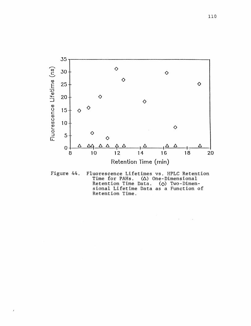
110
35
~ 0 (/) 30-c 0 "'--J
(}) 0 E 25 0
:;::; (})
0 ..._. 20 :.J 0 (}) 0 u 15 0 c I])
u (/) 1 0--(}) 0 '-0 0 :::J 5 lL 0
0- 6 ~ 6 6 ~6 16 '6 6 I . 6
8 10 12 14 16 18 20
Retention Time (min)
Figure 44. Fluorescence Lifetimes vs. HPLC Retention Time for PAHs. (6) One-Dimensional Retention Time Data. (O) Two-Dimensional Lifetime Data as a Function of Retention Time.

111
The above experiments verified that fluorescence lifetime
information on-line would indeed permit much more
selectivity for the determination of PAHs, thereby
affirming the initial goal of the research project: to
determine phase-modulation lifetimes on-line with HPLC.
On-Line Fluorescence Lifetime Determinations
The first use of a phase-modulation spectrofluorometer
is described for the measurement of fluorescence lifetimes
on-line with HPLC. Parameters such as mobile phase
composition and references used for lifetime calculations
were investigated, as well as the problems caused by
interfering signals.
Experimental
Stock solutions of PAHs were made up in 80% aqueous
MeCN. Sample solutions of PAH mixtures for HPLC runs were
made up with concentrations on the order of 1 X 10⁻⁶ M.
The Waters HPLC system was used in the isocratic mode with
a mobile phase of either 90% or 80% aqueous MeCN, and a
flow rate of 0.5 mL/min. The SLM 4800S was used along with
a modified, custom-made 20 ~L quartz flow cell (NSG
Precision Cells) for HPLC detection. A low-fluorescence
black quartz flow cell was also used for some experiments.
Fluorescence excitation wavelength was selected with the
excitation monochromator, while emission was observed with
long pass filters and a 600 nm short-pass filter. All

lifetime determinations were made using an excitation
modulation frequency of 18 MHz.
Effects of Solvent Composition on Lifetimes
112
The effect of changing solvent composition on the
fluorescence lifetimes of several PARs was determined. In
going from 100% MeCN and increasing the water content of
the solvent, the fluorescence lifetimes almost always
increase, as one would expect, and as illustrated for B(k)F
in Figure 45. As was discussed in Chapter III, this
apparent increase in the excited state lifetime is due to
the fact that molecules in excited electronic states
generally possess molecular geometries and electronic
charge distributions that are substantially different than
in the ground state. In most cases the excited state is
more polar than the ground state and an increase in solvent
polarity produces a greater stabilization of the excited
state (75) . To initially avoid another changing parameter,
the isocratic mobile phase was used.
Investigation of Possible Interferences
The presence of interfering signals was also
investigated, including scattered light, which is much
greater for microvolume flow cells than for conventional
cuvettes, fluorescence from filters, and solvent
impurities. The presence of solvent impurities can cause
both a relatively constant interfering background signal or

B(K)F
10.0 (/') z: z 9.0 1'---i
w :::E: I-I
1- 8.0 w LL. 1-1
-I
7.0
0 30 90
Figure 45. Lifetime vs. Percent Aqueous Acetonitrile as Solvent.
113

114
actual chromatographic peaks during a chromatogram. It is
important to note that, while for steady-state intensity
detection the constant fluorescence background can simply
be offset or "zeroed-out", for fluorescence lifetime
detection any fluorescence or scatter background will
influence the phase and modulation which is observed, and
therefore affect the calculated lifetimes . HPLC grade
MeCN from several suppliers were investigated (Fisher,
Mallinckrodt, Burdick and Jackson), and the Burdick and
Jackson MeCN was found to be consistently superior. Water
sources, including (1) distilled, de-ionized water directly
from an in-lab water distillation apparatus, (2) this same
water after passage through an activated charcoal column,
and (3) B&J water were investigated. The activated
charcoal-filtered water showed similar and only slightly
higher impurity than the B&J water and therefore was used
for further experiments. The long-pass filters that were
initially used in the experimental arrangement were
replaced by "low-fluorescence" long pass filters purchased
from Oriel. The remaining source of unwanted signal was
assumed to be due to scattered light. To solve the problem
of scattered light, several adaptations were made to the
flow cell and sample chamber, including the following: (1)
covering and eventual removal of the reflective mirrors on
the two sides of the flow cell mount; (2) addition of black
tape to the quartz block encasing the actual capillary
tube; and (3) construction of additional slits to be placed

115
in the sample compartment in order to further reduce any
stray light present in the system. Although these measures
helped in small amounts, scattered light was still found to
contribute to the signal detected. The approach was then
changed from attempting to physically reduce the scattered
light to mathematically correcting for it by treating it as
a component in a heterogeneous system.
Scattered Light Corrections
It was assumed that scattered light has a radiative
lifetime of zero and was the only source of unwanted signal
in the system. The fractional intensities of the scattered
light and the fluorescence emission were found from the
steady-state intensity information, since the scattered
light intensity is the intensity measured between
chromatographic peaks. The intensity of the fluorescence
signal at any point in a chromatographic peak was found
simply by subtracting the background scattered light
intensity from the total intensity, and the fractional
contributions of the scattered light and fluorescence
emission were then calculated.
As was discussed in Chapter 3, the observed phase
shift ~ and demodulation M for a two component system can
be expressed as follows (82):
tan ~ = S/G
M = [S2 + G2]1/2
(13)
(14)
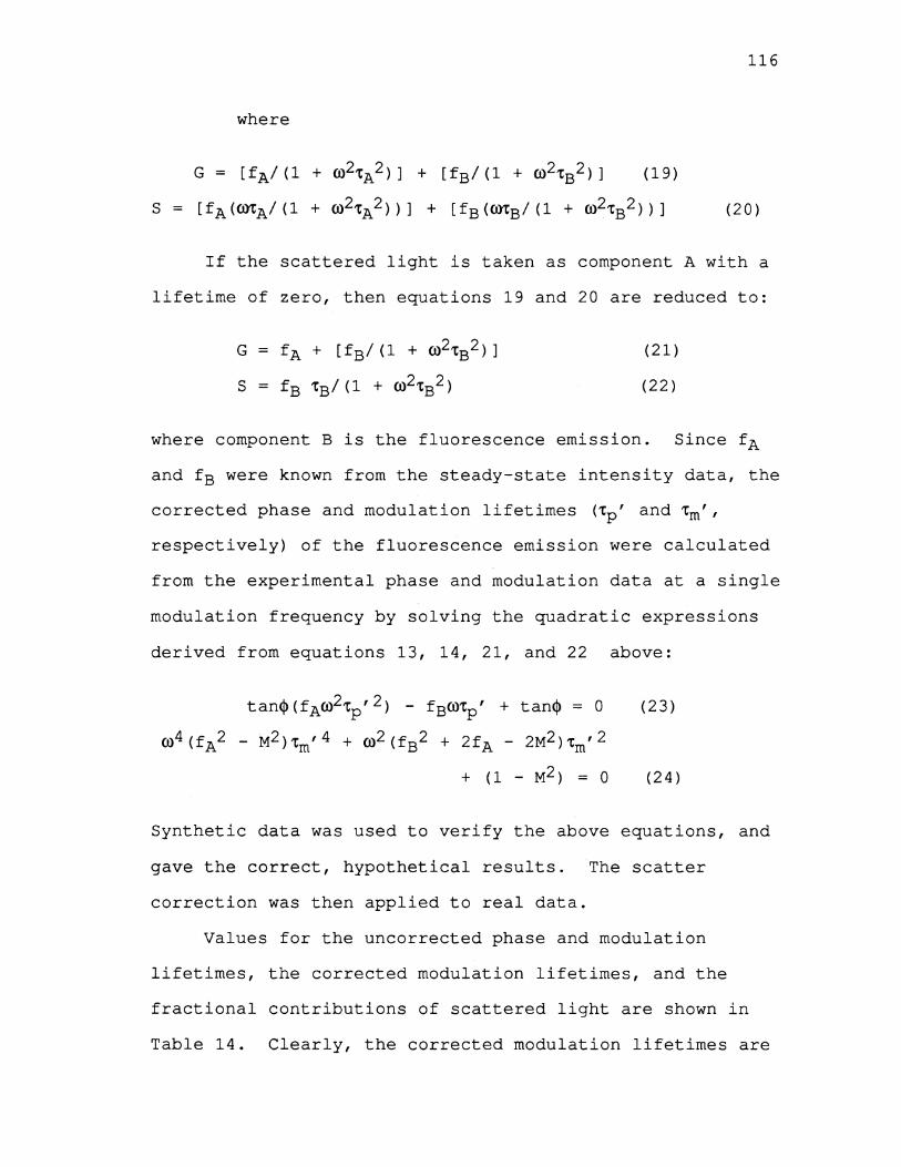
116
where
G = [fA/(1 + ro2tA2)] + [fB/(1 + ro2tB2)] (19)
S = [fA(~A/(1 + ro2tA2))] + [fB(~B/(1 + ro2tB2))] (20)
If the scattered light is taken as component A with a
lifetime of zero, then equations 19 and 20 are reduced to:
G = fA + [fB/ (1 + ro2tB2)]
S = fB tB/ (1 + ro2tB2)
( 21)
(22)
where component B is the fluorescence emission. Since fA
and fB were known from the steady-state intensity data, the
corrected phase and modulation lifetimes (tp' and tm',
respectively) of the fluorescence emission were calculated
from the experimental phase and modulation data at a single
modulation frequency by solving the quadratic expressions
derived from equations 13, 14, 21, and 22 above:
tan~(fAro2tp'2) - fBrotp' + tan~ = 0 (23)
ro4(fA2- M2)tm'4 + ro2(fB2 + 2fA- 2M2)tm'2
+ ( 1 - M2) = 0 ( 2 4)
Synthetic data was used to verify the above equations, and
gave the correct, hypothetical results. The scatter
correction was then applied to real data.
Values for the uncorrected phase and modulation
lifetimes, the corrected modulation lifetimes, and the
fractional contributions of scattered light are shown in
Table 14. Clearly, the corrected modulation lifetimes are

TABLE 14
FLUORESCENCE LIFETIMES FOR B(k)Fa
nb F c s t d m t , e m t f p
* 1. 000
1 .870 2.97 7.47 0.41
2 .810 3.47 7.03 0.74
3 .782 3.87 7.44 0.99
4 .790 3.90 7.73 0.96
5 .818 3.52 7.43 0.91
6 .853 3.21 7.64 0.74
7 .890 2.48 8.01 0.64
8 .922 2.37 7.93 0.40
9 .940 2.14 8.40 0.33
10 .958 1. 84 8.94 0.14
11 .966 1. 50 7.46 0.12
a Excitation = 380 nm; Emission = 385 nm LP. b Position along the chromatographic peak. c Fractional contribution of scattered light. d Uncorrected modulation lifetime. e Scatter-corrected modulation lifetime. f Uncorrected phase lifetime.
117
118
much closer to the expected 8.25 ns lifetime for B(k)F
under these conditions. Also, the corrected values are
essentially constant over the entire peak, which is
expected for a single component, since as soon as any
intensity is measured for a peak, it should have a single
lifetime value corresponding to that component regardless
of concentration. The uncorrected values, on the other
hand, rise and fall in a manner reflecting the
chromatographic peak shape, since the fractional
contribution of the second component (scattered light) is
decreasing and then increasing along the peak profile. The
wavelengths used to collect the data in Table 14 were very
close to the scatter peak in order to test the ability to
correct for large amounts of scattered light. Corrected
values are not shown for the phase lifetime because
meaningful values were not obtained under these conditions.
A second set of data for B(k)F was collected further away
from a scatter peak, and the results are shown in Table 15.
The corrected phase and modulation lifetimes are in good
agreement with each other and are fairly constant over the
peak, but the values are about one-half of the expected
lifetime for B(k)F. The scatter corrections definitely
improved the results for lifetime determinations, since
constant values were obtained across the peak. However,
some other factor was evidently also present which caused
inaccurate values to be calculated for the lifetimes.
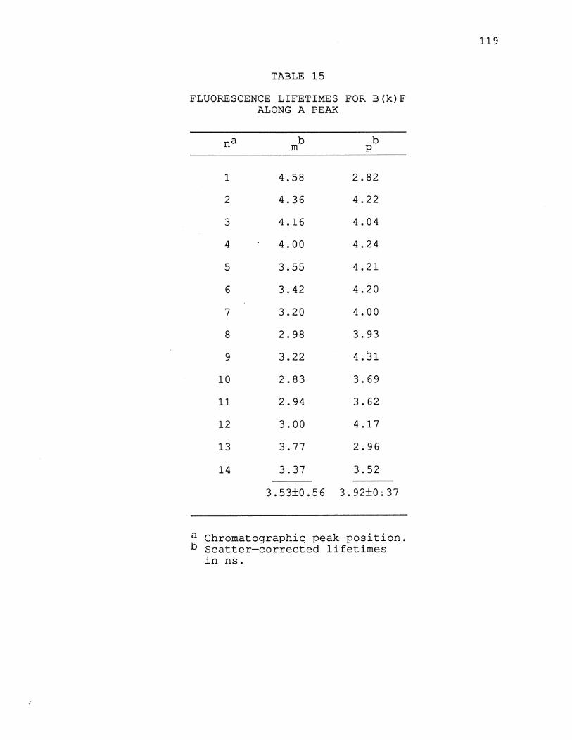
TABLE 15
FLUORESCENCE LIFETIMES FOR B(k)F ALONG A PEAK
na b b m p
1 4.58 2.82
2 4.36 4.22
3 4.16 4.04
4 4.00 4.24
5 3.55 4.21
6 3.42 4.20
7 3.20 4.00
8 2.98 3.93
9 3.22 4.31
10 2.83 3.69
11 2.94 3.62
12 3.00 4.17
13 3.77 2.96
14 3.37 3.52
3.53±0.56 3.92±0~37
a ChromatographiG peak position. b Scatter-corrected lifetimes
in ns.
119

120
Comparison of References
In a second set of experiments, steps were taken to
further reduce the amount of scatter interfering with the
analyte signal. A self-masking black-quartz flow cell with
a 20 ~L volume (Hellma Cells) was purchased. This cell was
specifically designed to block any stray light except that
which directly impinges on the observation volume. In
addition to the flow cell, the excitation wavelength used
was 360 nm with both a 399 nm low-fluorescence long-pass
filter and a 600 nm short-pass filter for emission. This
arrangement significantly reduced the scattered light
present in the experiment.
A mixture of five components, fluoranthene,
benzo(b)fluoranthene (B(b)F), benzo(k)fluoranthene (B(k)F),
benzo(a)pyrene (B(a)P), and benzo(ghi)perylene (B(ghi)P)
was investigated under mobile phase conditions of 80%
aqueous MeCN and a flow rate of 0.5 mL/min. The use of
dimethylPOPOP (t=l.45 ns) was compared to the use of
scattered light off of the flow cell as the reference. The
advantage of using the scatter from the flow cell as the
reference is that no additional compound needs to be added
to the mixture for the lifetime determinations. The
scatter from the flow cell was observed by removing the
filters from the emission path and collecting data for the
scatter under baseline chromatographic conditions.
The following figures show lifetimes vs. relative time
measurements taken across individual peaks. The zero point

121
indicates a point in time just before the peak is detected.
Figure 46 shows the lifetime vs. time for the five
completely separated compounds using the scatter reference.
Figure 47 shows the same using dimethylPOPOP as the
reference. The lifetimes acquired on-line with the HPLC
are reasonably constant, especially for the shorter-lived
components, and close to the values shown in Table 13
above. There are at least two reasons the lifetimes are
more constant for the shorter-lived components: first, the
modulation frequency used in this experiment was 18 MHz,
which is optimal for a lifetime of 8.8 ns; second, the
references, both the scatter {t=O) and the dimethylPOPOP
{t=1.45 ns), are very short-lived and therefore the
differences between the lifetimes of the references and the
analytes are less for the short-lived compounds. In
general, it appears that the lifetimes were more constant
when dimethylPOPOP was used as the reference, although for
all examples the lifetimes came together at the correct
value in regions close to the peak maxima.
The above sets of experiments identified many initial
problems related to acquiring lifetime data on-line with
HPLC. The scatter correction procedure is applicable not
only to the problems related to this particular
instrumental arrangement, but to any experiment where the
phase-modulation technique is being used to determine
lifetimes in a scattering environment such as front surface
fluorescence or other similar arrangements.

122
40
30
10
A-A-A A-t._
if[}-[>-~ A-
~~ (/) to z a b . (/)
40 w ~
tJ 30 lL
A-A 'Tm D-.D 'Tp ::::i w 10 0 z A -b.· ·.A.- .. A A "'"" .... - -.::< w u (/) w ~ 0 :::::> _j lL
tO
40
30
10
10
0 0
c
e
2
..... ~ 1111-tt-0-11-11 II d
2 4 • I 10 12
RELATIVE TIME
A-A-A-A-A-A· _... .. _A ..... ~ .... "Lr-0
4 I I 10 12 14
RELATIVE TIME
Figure 46. Lifetimes vs. Time Using Scatter as the Reference. (a) Fluoranthene, (b) B(b)F, (c) B(k)F, (d) B(a)P, and (e) B(ghi)P.
1 4

123
40
~
~-6-6-6-6 20 ~ (/) to z a b -(f) 40 w
:::e w 30 A-ATm o-o -rp 1.&.. ::J w 20 u fFDlla II ~A-A-A z w tO A=~ A a a 11 a-aa+-a
D-o-.o u c d (f) w a::: 40 0 2 4 • • 10 12 ::J RELATIVE TIME --' 1.&.. 30 > /A'
10 ~ 10 e
2 4 I I 11 12 14
RELATIVE TIME
Figure 47. Lifetimes vs. Time Using DimethylPOPOP as the Reference. PARs are the Same as in Figure 46.
14

Application of Phase-Modulation Fluorescence
Lifetime Determinations and Heterogeneity
Analysis To Mixtures of B(k)F and B(b)F
124
Steady state intensity information from compounds
separated by HPLC is useful for identification and
quantification; however, one must be reasonably convinced
that the peaks are due to only one component. Also, in
areas where more than one component is contained in a
chromatographic peak or peak portion, some means of
quantitation of those components must be available.
In this set of experiments the apparent lifetimes were
calculated from the phase-shift and demodulation of the
emission signal relative to the exciting light, as was
discussed in the fluorescence lifetime theory section
(Chapter 3, equations 9 and 10) . The degree of agreement
between the apparent phase and modulation lifetimes was
used as an indicator of chromatographic peak overlap, ie.,
the presence of more than one fluorescent component at a
given point along the chromatogram. Phase-modulation
fluorescence chromatograms collected at more than one
modulation frequency were used to perform heterogeneity
analysis, in which the fluorescence lifetimes and
fractional contributions to intensity of the components at
each point along the chromatogram were calculated.
The use of phase-modulation measurements for the
chromatographic detection of a binary system of
benzo(k)fluoranthene (B(k)F) and benzo(b)fluoranthene

125
(B(b)F) is described. Both on-line HPLC detection and
batch mode simulations were used to demonstrate the ability
of phase-modulation fluorometry to resolve the fluorescence
contributions of the two components in overlapping
chromatographic peaks. Solvent composition was varied in
order to create different degrees of peak overlap ranging
from zero to essentially complete overlap. B(k)F and B(b)F
were chosen for this work because of the similarity in
their chromatographic retention properties and their
spectral absorption and fluorescence characteristics. The
difference between their fluorescence lifetimes is large,
thereby facilitating the resolution of their
chromatographic peak intensity contributions by the use of
phase-modulation fluorescence detection.
Experimental
Stock solutions of B(k)F (5.07 X 10⁻⁵M) and B(b)F
(9.91 X 10⁻⁵ M) were prepared in 100% MeCN. Standards and
mixtures were prepared by dilution of the stock solutions.
The concentrations in the mixture used for HPLC were 2.38 X
10-6M for B(b)F and 1.50 x 10⁻⁶M for B(k)F. This
resulted in amounts injected of 11.5 ng and 7.6 ng for
B(b)F and B(k)F respectively. The HPLC separations were
performed with isocratic solvent systems of 75% and 90%
MeCN in water and 100% MeCN. Samples were manually
injected by syringe in 20 ~L volumes. Phase, modulation,
and steady state measurements were made with the SLM 4800S,
126
which was described in the general instrumentation section.
A 20 ~L self-masking black quartz flow cell (Hellma Cells)
was used in the fluorescence instrument. Excitation
wavelength was selected at 360 nm by the excitation
monochromator, and a combination of a 399 nm low
fluorescence long pass filter with a 600 nm short pass
filter (Oriel) was used to pass the fluorescence emission.
A kaolin (Aluminum Silicate) scattering solution was used
as the reference for batch fluorescence lifetime
determinations, and scatter from the flow cell without
filters in the emission path was used as the reference for
the on-line fluorescence lifetime determinations.
Solutions were not deoxygenated.
The phase-modulation chromatographic and batch
simulation experiments were all performed as five replicate
runs, and the results are expressed as the averages of the
runs. Chromatographic data and batch simulation data was
collected with fluorescence detector in the ''10 average"
mode, and fluorescence lifetime determinations in the batch
mode were performed in the "100 average" mode.
Heterogeneity analysis using Weber's algorithm was
performed on an APPLE IIe computer using the SLM software.
Weber's algorithm requires only two modulation frequencies,
so results for Weber's algorithm shown in this experiment
are for 6 MHz and 18 MHz data, which was found to give the
best overall results for the B(k)F/B(b)F system. The
nonlinear least squares (NLLS) heterogeneity analyses were

127
performed on an IBM PC-AT, also using SLM software. Data
for the NLLS analyses was acquired at all three modulation
frequencies (6, 18, and 30 MHz). In cases for which the
NLLS program suggested a one-component solution, both the
one-component and two-component solutions were found. Only
the two-component solutions are reported here, as the one
component solutions did not give any overall improvement in
the results.
Batch Experiments
A series of six solutions in 100% MeCN were studied in
a batch mode, in order to test the ability of the
heterogeneity analysis experiments to resolve the
contributions of B(k)F and B(b)F in mix~ures of the two.
The solution compositions were chosen to represent the
relative fluorescence intensity contributions of B(k)F and
B(b)F, represented by aA and aB, respectively, at
successive points along a chromatogram. Measurements of
phase-shift and demodulation for each sol~tion at 6, 18,
and 30 MHz were used to calculate tp and tm values at each
frequency. Heterogeneity analyses were then performed to
find aA, aB, tA, and tB, using both Weber's algorithm for
exact solutions and the NLLS approach. Results, expressed
as the relative errors in the a and t values for each
component, are shown in Table 16. Results are also shown
in Table 16 for NLLS analyses in which the fluorescence

TABLE 16
RESULTS FOR BATCH HETEROGENEITY ANALYSIS FOR B(k)F ~~D B(b)F
% Error
Exact (6,18 MHz) NLLS1 (6,18,30 MHz) NLLS2 (6,18,30 MHz)a
True Value TA a A TB aB I TA a A TB aB I a A aB
a A aB
o. 77 0.23 -2.5 -4.8 -5.0 22 -2.6 -4.2 -4.4 21 0 5.3
0.58 ·o. 42 -3.9 -3.2 -4.5 11 -0.9 1.7 2.1 3.5 3.2 1.2
0.36 0.64 -6.1 -8.0 -1.5 8.9 2.0 3.7 5.3 4.3 -0.3 -2.0
0.19 0.81 -7.1 -7.3 -0.4 3.4 13 25 7.2 5.8 -1.3 0.7
0.08 0.92 -12 -16 0.2 1.0 -- -100 -16 8.7 I -12 0.5
0.04 0.96 -32 -32 -0.8 1.4 -- -100 -8.7 4.3 -16 0.5
a NLLS2 performed as with NLLS1 but with TA and TB fixed at 7.23ns and 25.24ns.
..... N ro

lifetimes of the two components were fixed at the values
obtained for the B(k)F and B(b)F standard solutions.
Chromatographic Experiments
129
The chromatographic resolution of the B(b)F and B(k)F
peaks is listed in Figure 48 for each of the three solvents
used (75, 90 and 100% MeCN). Resolution R was calculated
as the difference between the retention times of B(k)F and
B(b)F, divided by the mean of the two peak widths. The
resolutions for the UV absorption chromatograms were
slightly greater than those of the fluorescence
chromatograms, probably due to the positioning of the
fluorometer after the absorption detector. The peaks were
completely resolved with 75% MeCN, partially resolved with
90% MeCN and highly overlapping with 100% MeCN, as is also
shown in Figure 48.
Six chromatograms (each the average of five
replicates) were run for each of the three solvent
compositions, including the steady state fluorescence
intensity chromatograms of the individual B(k)F and B(b)F
solutions and the B(k)F/B(b)F mixture, and the phase
modulation fluorescence chromatograms of the mixture at 6,
18 and 30 MHz modulation frequencies. Retention time
reproducibility was within 1.3% relative standard deviation
for each of the sets of five replicate chromatograms.
Steady state fluorescence intensity chromatograms of the
two individual components were constructed from the phase-

Solvent
a) 75/25
b )90/10
c)l00/0
Detector R
A 2.0
F 2.0
A 0.83
F 0. 72
A
F
0.53
0.41
130
c b a
- c -"\
Figure 48. Chromatograms of B(k)F and B(b)F Using Different Mobile Phase Compositions ~vith Isocratic Elution.

131
modulation chromatograms of the mixture as follows. The
phase-shift and demodulation values recorded at each point
along the phase-modulation fluorescence chromatograms were
used to calculate the tp and tm values at each point,
yielding three sets of tp and tm values per point (one set
for each modulation frequency) . Heterogeneity analysis of
the fluorescence lifetime data was then used to find aA,
aB, tA and tB at each chromatographic point. The steady
state fluorescence intensity chromatograms for each
component were constructed by multiplying the a value for
the component at each point by the steady state intensity
of the mixture chromatogram at that point. The re
constructed chromatograms were compared at each point with
the steady state intensity florescence chromatograms of the
individual components. The comparison was based on three
criteria: the retention time <tr), the fluorescence
intensity (Ip), and lifetime (tp) at the peak. Results are
summarized in Table 17 for both the exact solutions and
NLLS analyses, in terms of the relative errors for each of
the comparison criteria.
Discussion
The batch simulation experiments show the limiting
accuracy that can be expected in resolving the fractional
intensity contributions of B(k)F and B(b)F in 100% MeCN
with the SLM 4800S. The accuracy with which the
fluorescence lifetimes can be determined is also indicated.

RELATIVE ERRORS
Solvent (%MeCN/ %Water)
75/25
90/10
100/0
Method
Exact a
NLLS1b
NLLS2c
Exact
NLLS1
NLLS2
Exact
NLLS1
NLLS2
tr
1.5
-3.0
-1.9
-0.5
-0.9
-0.6
1.3
2.5
0.8
Average I% errorl :d
Exact 1.1
NLLS1 2.1
NLLS2 1.1
FOR
132
TABLE 17
ON-LINE HETEROGENEITY ANALYSES
B(k)F B(b)F
IF 'tF tr IF 'tF
8.5 0.4 4.0 9.2 6.3
15.8 0.7 -0.3 -12.6 -9.6
7.9 -5.7 -12.8
23.4 2.2 0.8 -1.2 -17.1
16.8 16.8 0.1 2.1 -10.4
23.1 0.0 -4.3
16.2 -1.5 -2.1 -16.7 -9.2
18.7 14.6 -1.1 -8.6 -8.9
9.3 -1.3 -12.1
16.0 1.7 2.3 9.0 11.0
17.0 11.0 0.5 7.8 9.6
13.0 2.3 2.3
a Exact solution using Weber's algorithm at 6 and 18 MHz. b NLLS1 performed at 6, 18, and 30 MHz. c NLLS2 perfomed at 6, 18, and 30 MHz with lifetimes fixed. d Relative error magnitude averaged for the three solvent
systems.

133
As would be expected, the accuracy of the fluorescence
contributions and lifetime determinations decreases as the
fractional intensity contribution of the component
decreases. The magnitudes of the relative error for the
exact solutions systematically increase, whereas the NLLS ·
errors show random fluctuations except for the extreme
cases of aA>>aB or aA<<aB, for which the errors show a
sharp increase.
For the chromatographic experiments, the relative
errors in florescence contributions and lifetimes are
lowest at the points in the chromatograms corresponding to
the peaks of the components. The errors increase as the
peripheral regions of the peaks are approached, as expected
both intuitively and from the results for the batch
simulations. For analytical purposes, the retention times
and the fluorescence intensity and lifetime values at the
chromatographic peaks of the components are of the most
value in both quantitative and qualitative analysis.
Several interesting points can be made about the
results shown in Table 17. Very good results were obtained
for the retention times of the peaks that were constructed
from the phase-modulation data. Errors in retention time
were largest for the 75% MeCN, despite the fact that
complete chromatographic separation is obtained with this
solvent system. This indicates that the error is related
to the magnitude of the retention time itself, which is
much longer for the 75% MeCN solvent, rather than to the

134
errors in the phase-modulation reconstruction of the peaks.
There appear to be systematic errors (positive for B(k)F
and negative for B(b)F) in the peak intensity and lifetime
determinations. The errors do not seem to be related to
chromatographic resolution, i.e., errors do not decrease as
the chromatographic separation improves. Overall, the
exact solution results for B(k)F are better than the NLLS
solutions, especially for the ~F determinations in which
the average magnitudes of the relative errors differ by an
order of magnitude. On the other hand, the NLLS results
(with variable ~A and ~B) are somewhat better than the
exact solution results for B(b)F. These apparent biases
may be the result of the modulation frequencies used for
the experiments, since Weber's algorithm and the NLLS
program weight the errors in the phase and modulation
differently.
Fluorescence Lifetimes for PAHs On-line
With HPLC Using A Multifrequency
Phase-Modulation Fluorometer
The first use of a multifrequency phase-modulation
fluorometer is described for the measurement of
fluorescence lifetimes on-line with HPLC. Several
considerations were addressed, including correction factors
for instrumental problems, intensity matching of the
reference and sample signals, and the effect of changing

the HPLC flow rates and mobile phase composition on the
observed fluorescence lifetimes obtained.
135
As was noted in the previous section, there are
several features of fluorescence lifetime measurements that
are of particular importance for HPLC detection. First of
all, fluorescence lifetime is generally independent of
concentration; therefore, the lifetime for a single
component peak should attain a certain value as soon as the
fluorescence intensity is detected, and remain constant
over the entire peak. Second, phase-modulation lifetime
determinations provide two independent lifetime values: tp,
calculated from the phase-shift, and tm, calculated from
the demodulation. For single-component peaks, tm has the
same, constant value as tp over the entire peak. For
overlapping peaks, on the other hand, tm will be greater
than tp in the regions that are comprised of more than one
fluorescent component. Phase-modulation fluorescence
lifetime detection can therefore be used to indicate the
presence of more than one fluorescent component at any
point along the chromatogram.
Experimental
Stock solutions and samples were prepared as described
in the general experimental section. Samples were manually
injected by syringe in 20 ~L volumes. Isocratic elution
was again used in this work, and the mobile phase
compositions will be described later. A four-port valve
136
was used to connect the flow between the UV absorption
detector and the fluorometer, in order to perform stopped
flow experiments. The valve had no noticeable effects on
the chromatographic peak in the continuous flow
experiments, and was therefore left in place for all HPLC
experiments. The 20 ~L self-masking black-quartz
fluorescence flow cell was used for flow and stopped-flow
measurements.
Fluorescence lifetimes were determined on the SLM
48000S multifrequency phase-modulation spectrofluorometer
(SLM Instruments, Inc.), described in the general
instrumental section (Chapter 4), in which electrooptic
modulation is used to provide essentially continuous
frequency selection in the 1 - 250 MHz range. Wavelength
selection was accomplished with the excitation
monochromator set at 360 nm and a combination of a 399 nm
long-pass and a 600 nm short-pass filter for emission. For
batch measurements, 10 75-average measurements were used.
The "slow time kinetics" mode of the instrument was used to
acquire data with time under flow conditions. On-line
measurements were acquired as a 3-average reading taken
once per second. The raw data, including d.c. intensity,
a.c. amplitude, and phase angle, was transferred to a
spreadsheet (As Easy As, shareware) program for data
manipulations. Scatter was used as the reference for the
batch lifetime calculations, while 9-anthracenecarbonitrile

137
(9-AC, 97%, Aldrich) was used as the reference for the on
line work.
Batch Analysis
A batch heterogeneity analysis of B(k)F I B(b)F was
repeated with the 48000S multifrequency instrument in order
to determine how the new instrument compared with the 4800S
used in previous experiments. Fluorescence lifetimes were
obtained for several solutions containing mixtures of B(k)F
and B(b)F. The concentrations and relative steady state
fluorescence intensities are shown in Table 18. Excitation
modulation frequencies used included 7, 15, 23 and 35 MHz.
Table 19 shows the fluorescence lifetimes obtained at each
frequency for each solution. Non-linear least squares
(NLLS) heterogeneity analysis was used to determine the
lifetimes and fractional contributions of each compound in
each solution, and these results are shown in Table 20.
Table 20 also shows the results when the lifetimes were
fixed at 7.05 ns (B(k)F) and 24.89 ns (B(b)F). Overall,
the errors are low and only get prohibitively large for the
minor component when the fractional contributions get below
20%. The errors were significantly reduced for the
fractional contributions when the lifetimes were fixed, as
would be expected. The use of multifrequency
instrumentation significantly improved the results for
heterogeneity analysis over those using the 4800S where
only 6, 18, and 30 MHz were available (compare Table 20 to

138
TABLE 18
MIXTURES OF B(b)F AND B(k)F FOR HETEROGENEITY ANALYSIS
Concentration Concentration Relative B(b)F (M) B(k)F (M) Intensity
1 2.06 X 10⁻⁶ .6094
2 1. 31 x 10-7 1. 80 x 1o-6 .6179
3 2.41 x 10⁻⁷ 1.55 X 1o-6 .6036
4 3.73 x 1o-7 1.29 X 10⁻⁶ .5891
5 4.84 x 1o-7 1.04 X 1o-6 .5936
6 6.17 x 1o-7 7.78 x 1o-7 .6021
7 7.28 x 1o-7 5.19 x 1o-7 .5878
8 8.62 x 1o-7 2.60 x 1o-7 .5863
9 9.96 X 10⁻⁷ .5871

139
TABLE 19
FLUORESCENCE LIFETIMES OF MIXTURES OF B(b)F AND B(k)Fa
Freq. 1 2 3 4 5 6 7 8 9
7 tp 24.78 20.93 17.96 15.58 13.61 11.60 9.96 8.44 7.19
tm 24.99 23.73 21.77 20.04 18.22 15.66 13.02 9.86 5.60
15 tp 24.70 17.80 14.49 12.22 10.75 9.47 8.50 7.72 7.16
tm 24.93 22.08 19.74 17.09 14.98 12.67 10.69 8.69 6.73
23 tp 24.54 15.97 12.76 10.88 9.69 8. 71 8.09 7.50 7.18
tm 25.00 20.98 17.93 15.42 13.43 11.36 9.74 8.20 6.91
35 tp 24.91 14.79 11.82 10.11 9.13 8.38 7.90 7.43 7.18
tm 24.97 20.09 16.74 14.31 12.40 10.60 9.23 7.95 6.97
a Lifetimes (in ns) calculated from the phase-shift and demodulation for each of the nine mixtures.

140
TABLE 20
RESULTS OF BATCH NLLS HETEROGENEITY ANALYSIS
% Error "True" F1 "True" F 2
# (B(k)F) (B (b) F) F1 't1 F2 't2 F1'a F2'a
1 0.00 1. 00
2 0.13 0.87 7.7 6.2 0.0 2.0 -7.7 2.3
3 0.24 0.76 -4.2 -6.0 0.2 -1.3 0.0 0.0
4 0.37 0.63 -5.4 0.6 0.0 -1.2 -2.7 -1.5
5 0.48 0.62 -4.2 -0.3 3.8 -2.9 -2.1 1.9
6 0.60 0.40 0.0 0.9 5.3 -4.3 0.0 5.3
7 0.73 0.27 -1.4 0.3 7.7 -10.4 0.0 3.8
8 0.87 0.13 -2.3 -0.3 15.4 -22.9 0.0 0.0
9 1. 00 0.00
a NLLS performed with t 1 and t 2 fixed at 7.05 ns and 24.89 ns.

141
Table 16 in last section). Due to the multifrequency
capabilities of the SLM 48000, the 250 frequencies (vs. 3
on the SLM 4800S) provide for much superior optimization in
the number and selection of frequencies.
Fluorescence Lifetimes On-line With HPLC
Initial investigations. Fluorescence lifetimes were
obtained on-line with the HPLC. The figures for all of the
continuous-flow experiments represent relative time on the
x-axis. It should be noted that zero on the relative time
scale refers to a point just prior to elution of the peak,
and does not indicate zero retention time.
It was determined that the use of the scatter from the
flow cell was very dependent on the exact positioning of
the flow cell, and also gave consistently poorer results
(tm=tp) than when a reference fluorophore was used. 9-AC
was chosen as the reference fluorophore since its lifetime
(t=11.31 in 100% MeCN) and spectral characteristics were in
the same general range as most of the PAHs under
investigation.
Figure 49 shows the fluorescence vs. time data for
B(k)F at 0.5 mL/min and 100% MeCN. As can be seen,
although the phase lifetimes are fairly constant over the
peak, the modulation lifetimes are not only delayed but
also highly sloping. Several experiments were done to
determine if this behavior might be due to scattered light
present in the system. Scatter corrections, described in

14
ll. 2
8. 4
:J
~ 5.6
2.8
0
+'
0
.+. '+. ~
3
142
....... TouM -a- TouP ·+ rei int
"+. '+. ...... ·+ .
··+··+··+· ·+··+
6 9 . 12 15 TimQ
Figure 49. Fluorescence Lifetime Chromatogram for B(k)F at 0.5 mL/min and 100% MeCN.

143
the section ("On-line Fluorescence Lifetime
Determinations"), were applied here as well as the use of
crossed polarizers was investigated to cut out the scatter.
These experiments all failed to improve results.
Intuitively, it would seem that if scattered light were the
problem, both the phase and modulation lifetimes at the
peak periphery would fall to lower values because of the
increasing contribution of the zero lifetime scatter. This
is obviously not the case and therefore it was determined
that scattered light was not the problem in this
experimental arrangement.
Next, the possibility that the poor lifetime response
was due to flow effects such as mixing in the flow cell was
investigated. If the problems were caused by mixing in the
flow cell, or by absorption of PARs on the flow cell walls,
then the response of the fluorescence lifetimes should
change when the HPLC mobile phase flow rate was varied or
when the mobile phase composition was changed. In order to
test this hypothesis, the fluorescence lifetimes on-line
were determined at flow rates from 0.2 mL/min to 1~2 mL/min
with 100% MeCN. These are shown graphically for 0.2, 0.4,
0.6, and 0.8 mL/rnin in Figures 50 and 51. Besides the
expected changes due to the sharper peaks at higher flow
rates and therefore fewer points per peak, all the flow
rates showed a similar response. The effect of changing
the mobile phase composition while keeping the flow rate
constant was determined for B(k)F and B(b)F at 0.5 mL/min.

14
11. 2
8. 4 ;:) 0 1-
5.6
2.8
~ tm
-e- tp ·+ rQ) int.
+ +·+ +" +·+. +" + ....
+ +.+ . + 0
.+ +·+ + +++ ·+++++·++·++·+
0 6
14
11. 2 (b)
8.4 ;:)
~ 5.6
2. 8 .+. ·+. . +"
+ 0
0 3
12
"+ . '+
6
18 Tlmo
. "+. "+ .. +·.
9
Tlmo
24
+·. +. ·+. ·+. ·+
12
Figure 50. Fluorescence Lifetime Chromatograms of B(k)F Using 100% MeCN at (a) 0.2 and (b) 0.4 mL/min.
30
IS
144

14
~ tm 11.2 -e- tp
·+ rel int
8. 4
:J 0 r-
5. 6
2. 8 .... (a) . . . ·+ .+ +.
.+" ·+. ·+ 0 +' . ·+· ·+·. +·. +
0 3 6 9 12 IS
Tlma
14
11. 2
8. 4
~ 5. 6
2. 8 ..... '+ (b)
+ '+. 0 '+· '+ .. +·. +
0 3 6 9 12 15
Tlma
Figure 51. Fluorescence Lifetime Chromatograms of B(k)F Using 100% MeCN at (a) 0.6 and (b) 0.8 mL/min.
145
146
As can be seen in Figures 52-54, the only differences which
can be seen in going from 100 to 80% MeCN is the peak
broadening. Methanol was also used in place of the MeCN
and gave very similar results. The incorrect behavior of
the lifetimes, especially the modulation lifetimes, was
shown not to be due to the presence of scatter, dynamic
mixing, the particular compound, absorption effects, or
other effects which can be traced to the analytes or to the
solvent and solvent delivery. To determine if the effects
could be tied to physical or mechanical problems instead of
chemical problems, a series of experiments were done to
pinpoint the exact cause of the incorrect lifetime behavior
under flowing conditions.
Batch Mode Simulations. B(k)F was incrementally added
to 100% MeCN in a quartz cuvette in order to simulate the
concentration profile of the front edge of a
chromatographic peak. Fluorescence intensity and phase and
modulation lifetimes for each of the solutions are shown in
Figure 55a. Over most of the "peak" edge, 'tp = 'tm = 7 ns,
as expected for a peak containing B(k)F ('t 7 ns).
However, 'tm was increasingly greater than 'tp as the
intensity decreased (approaching the front of the "peak").
Since these measurements were under batch conditions, flow
is not responsible for this effect. Further studies
indicated the importance of intensity matching between the
reference 9-AC solution and the sample. All of the
lifetimes shown in Figure 55a were obtained by calibration

14
11. 2
B. 4 :I
~ 5.6
2. B (a)
0
0
... TcuM -8- TcuP
6 9 12 15
Tlmo
9 12 15 Tlmo
Fluorescence Lifetime Chromatograms at 0.5 mL/min and 80% Aqueous MeCN for (a) B(k)F and (b) B(b)F.
147

J.4
11.2
B. 4 :;:) D 1-
5. 6
2. 8 (a)
0
0
so
40
30 :I D t-
20
10 (b)
0
0
Figure 53.
* TauM -e- TauP
3 6 9 12 15
Timg
3 6 9 12 15
Timg
Fluorescence Lifetime Chromatograms at 0.5 mL/min and 90% Aqueous MeCN for (a) B(k)F and (b) B(b)F.
148

::J {!.
14 ... TauM 1 1. 2 -e- TauP
e."
5. 6
2. 8 (a)
0
0 3 6 9 12 IS Tlmo
50
40
30
::J 0
1-
20
10 (b)
0
0 3 6 9 12 15
limo
Figure 54. Fluorescence Lifetime Chromatograms at 0.5 mL/min and 100% MeCN for (a) B(k)F and (b) B(b)F.
149

25
....--.. (a) en o-o Tau Phase c
'-"' 20 6-6 Tau Mod Q)
Intensity E :;:::;
Q) 15 '+-
~ Q)
u c 10 Q) 11.....6-A..... u 6-6-6 en -6-6-~~~~g,.Q-6--I!t-lil=fr&o: -liF~W=Q::Q=Q=Q=g Q) o-0-o"D-o-o-D-tY ~
5 0 :J
LL
0 0 5 10 15 20 25 30
Solution Number
25
....--.. (b) en
c '-"' 20
Q)
E ....... Q) 15 '+-
~ Q)
u c 10 Q)
u 0 [] en ~ 6 :!>f!< 6)tr-tH!kw:=2::~&o:g::Q::Q=R=lir-Q=R=:&o:g; -lii=Q=W=Q::Q=Q=g::g Q) ~
5 0 :J
LL
0 0 5 10 15 20 25 30
Solution Number
Figure 55. Batch Fluorescence Lifetime Chromatogram Simulat'ions for B (k) F (a) Before and (b) After Reference Intensity Matching.
150
::u Cb
0 ,-+
<' Cb
:J ,-+
Cb :J (/)
,-+
'<
:;:u Cb 0 !:!: < Cb
::J r+ Cb ::J IJl ;:;: '<

151
with a 9-AC solution that had an intensity similar to that
of the highest concentration B(k)F solution. For these
conditions, intensity matching is not important until the
B(k)F intensity gets close to zero, at which point tm and
tp become increasingly divergent. Figure 55b shows the
improvement in lifetime determinations that is obtained
when calibration is performed with a 9-AC solution that has
the same intensity as the sample. Agreement between tm and
tp occurs over the entire concentration range, yielding the
correct value of 7 ns. The increase in random fluctuations
of the observed lifetimes at the low intensity edge is due
to the increased noise associated with the detection of
low-level signals.
Stopped-flow Simulations. The next experiments used
stopped-flow conditions to measure B(k)F as it was eluted
from the HPLC, in order to evaluate the effects of the flow
cell (but not flow conditions) on the lifetime
determinations. The stopped-flow experiments used the same
instrumental configuration as would be used for real-time
chromatographic detection, but the flow from the HPLC was
stopped for every measurement in order to eliminate effects
due to flow. First, a single 9-AC reference solution, with
an intensity similar to that of the B(k)F peak maximum, was
used for lifetime calibration of all points. As shown in
Figure 56a, there is excellent agreement between tp and tm
across most of the chromatographic peak, and the only
deviation occurs at the peak peripheries. Intensity-

152
25 ,..-...
(a) 1/) o-o Tau Phose c ............. 20 a-a Tau Mod
Ql Intensity ;o E (1)
......- 0 Ql 15 ....... - <' :.:J (1)
Ql /A :J (,) A-A ....... c 10 (1)
Ql A/ :J (,) / (J) 1/) _.,Ito ;::;.: Ql D-~0 '< L..
5 0 :J
u...
0 0 5 10 15 20 25
Sampling Position
25 ,..-...
(b) 1/)
c 20 .........
Q) :::::0 E (1)
:;:i 0 Ql 15 !:!: - < :.:J (1)
Ql :J (,) ,..... c 10 Cb Ql :J (,)
~<Y~o (J)
1/) ;:::;.: Ql '< L Ito A 0 5 IJ,/ :J
u...
0 0 5 10 15 20 25
Samplin'g Position
Figure 56. Stopped-Flow Fluorescence Lifetime Chromatogram Simulations for B(k)F (a) Before and (b) After Reference Intensity Matching.

153
matching helped to alleviate the deviation (Figure 56b) .
From this study, it was apparent that the flow cell itself
introduced no new problems or artifacts in the intensity or
lifetime determinations.
Flow Experiments. From the above batch and stopped
flow simulations it was clear that the lifetime response
vs. intensity followed theory and the flow cell did not
produce any serious problems for the lifetime
determinations. These results, along with previous ones
indicated that the problem was most likely due to an
instrumental artifact rather than being due to something
derived from the HPLC-imposed conditions.
To determine nature of the problem, both the a.c.
intensity and the d.c. intensity were observed on-line
under flowing conditions. This information was
investigated due to the fact that the modulation lifetimes
were the ones that were causing the problems, and the
modulation lifetimes are calculated from the modulation
ratio (a.c./d.c.) (see Figure 21). Figure 57 shows the
a.c. and d.c. intensities for B(k)F at 23 MHz along with
the modulation ratio (a.c./d.c.). The a.c. signal should
be directly alligned the d.c. signal, and there should be a
constant ratio of the a.c. to d.c. signals through the peak
in order to get constant modulation lifetimes. Obviously,
the a.c. signal is somewhat delayed, relative to the d.c.
signal. Figure 57 also shows the modulation ratio after
shifting the a.c. intensity to the left. A much flatter

3T-------------------------------------------~
~ Ul 2 z w 1--z w > ~ 1 w a:::
A- -A a.c. - a.c./ d.c. uncorrected
c-c d c . . -- a.c./ d.c. corrected
o------.. ~L---4---~~~----~
154
150 175 200
RELATIVE TIME
225 250
Figure 57. Dynamic (a.c.) and Steady-State (d.c.) Intensities and Modulation (a.c./d.c.) vs. Time for B(k)F.
155
"plateau-like'' response is obtained after aligning the a.c.
and d.c. peaks. The same shift is required for any data
collected under the same conditions (number of points
averaged, time step increment) .
The cause of the problems was initially difficult to
determine, but once we knew that it was caused by the fact
that the a.c. signal is acquired by the electronics at a
slightly later point in time than the d.c. signal, the
problem was easily corrected. The reason the manufacturer
was not aware of this problem is because the dynamic
(lifetime) mode of the instrument was designed to be used
only for static measurements, where the intensity would not
significantly change with time. Our results were
eventually confirmed by George Mitchell, the instrument
electronics designer for SLM.
Figure 58 shows intensity and lifetimes, collected
under flow conditions, for fluoranthene (~ = 29 ns) that
was eluted from the HPLC with a 100% MeCN mobile phase at a
flow rate of 0.3 mL/min. The results shown in Figure 58a
indicate two separate effects. First, this run used a
single 9-AC reference instead of intensity matching,
causing the lifetime divergence at the peak peripheries.
Second, the modulation lifetime is not symmetric about the
chromatographic peak and has a high, positive error at both
the front and tail edges of the peak. Figure 58b shows the
same data as for Figure 58a above, but with the a.c.
intensity shifted 0.4 seconds to correctly line up with the

156
60 A
,........,
(a)\ o-o Tau Phose I en a-a Tau Mod c 50
~ Intensity /1(' <l.l
/j ::u
E 40 \ (l)
:z 0 <l.l 6 ,.....
'+- ' <' ::J 30 0- i-6 C1l
<l.l ::J u A-~~~~0... ,..... c (l) <l.l
20 ~ ::J
u [/) en ;::+ <l.l '< L 0 10 ::J
u_
0 0 5 10 15 20 25 30
Relative Time (s)
60 ,........,
(b) en c 50 ~
<l.l ::u E 40
(l)
-I-' 0 <l.l
,..... '+- <' ::J C1l
<l.l 30 ~ ~ 0 0 ~ ::J u ..:.._,.,·""'·'a--Vi ,.... c /A._ (l)
<l.l 20
::J u [/)
en 6, ,..... <l.l 6 '< L 0 10 ::J
[i:
0 0 5 10 15 20 25 30
Relative Time (s)
Figure 58. Fluorescence Lifetime Chromatograms for Fluoranthene at 0.3 m.L/rnin and 100% MeCN (a) Before and (b) After Reference Intensity Matching and a.c. Correction.

157
d.c. signal, and with intensity matching of the reference
to the analyte. To determine the correct amount to shift
the a.c. signal under a particular set of experimental
conditions, the a.c. and d.c. intensities for the
chromatogram were collected. Using the "Edit a Spectrum"
feature on the SLM software, the a.c. intensity
chromatogram was shifted until it most closely aligned with
the d.c. intensity chromatogram. The ratio of the two was
then performed and the data manipulation continued. Once
the required shift was found for a particular set of
conditions, it was constant and did not need to be
determined again.
The reference intensity matching was done by taking
several stopped-flow measurements (intensity, phase, and
modulation) of the reference fluorophore as it was eluted
from the HPLC. The intensity of these stopped-flow
measurements was then matched with the particular points in
the chromatogram and the lifetime was calculated. This
intensity matching was first done by hand, later by a
search routine in the "As Easy As" spreadsheet program, and
eventually by a program written in Microsoft Quickbasic.
Effects of Flow Rate and Mobile Phase Composition. In
order for the on-line determination of lifetimes to be
generally useful, the lifetime determinations must not be
seriously degraded or changed with changes in HPLC mobile
phase flow rate or mobile phase composition. Figure 59
shows the fluorescence lifetimes vs. time with changing

158
30
" 25 (o) a-a Tau Pha•e (b) s •-• Tau Mod
" - lnten•ity :u E .. . .., 20 !i " :s <" .. .. 15 :; 0
" 1: •• 10 " u ~ . ., .:; .. ...
0 5 ::J G:
0 ~
0 5 10 15 20 25 JO JS •o •s 50 I 5 10 15 20 25 30 J5
Relative Time (!) Relative Time (!)
JO - {c) {d) .,
25 ..s .. ::0 E 20
.. . ., ~ ..
:3 <. .. .. 15 :; u ;; c
\X/ I .. 10 " u !!. .. .:; .. ...
0 5 ::J G:
0 0 5 10 15 20 ' 5 10 15 20
Relative Time (!!!) R~lotlve Time ( ")
Figure 59. Fluorescence Lifetime Chromatograms for B(k)F With 100% MeCN at (a) 0.3, (b) 0.5, (c) 0.8, and (d) 1.0 mL/min.

159
mobile phase flow rates. The mobile phase was 100% MeCN
and the data points were taken one every second. Relative
to a flow rate of zero (stopped-flow), all of the flow
rates used for on-line lifetime determinations exhibited
increased noise that is especially evident at the edges of
the peaks. As flow rate through the HPLC was increased,
fewer points were collected per peak and the quality of the
lifetime data was degraded. The best data was acquired at
0.3 mL/min, with systematic divergence at the higher flow
rates. Figure 60 shows the results when the flow rate was
held constant at 0.5 mL/min and the percent MeCN in water
was varied for the mobile phase. Best results appear to be
for the 90% MeCN chromatograms.
The effects of both flow rate and mobile phase
composition can be attributed to similar causes. The
systematic divergence of tm and tp, which increases with
increasing flow rate or decreasing retention, appears to be
related to the resulting increase in slope across the peak;
this may be due to the difficulty in exactly compensating
for the a.c. delay, which is more critical at higher
slopes. The decrease in precision, which occurs with
decreasing flow rate or increasing retention, appears to be
related to the expansion of low-intensity regions that
results from peak broadening.
In general, the fluorescence lifetimes were acceptable
under all conditions investigated. There were errors at
the higher flow rates; however, it must be noted that the

30 ...... n r 25
"' .g 20 .!! :.J
IS .. u c .,
10 u n ., ... 0 5 " G:
0 0 10 20 30
30 ...... n
25 .s .. . § 20 c; :5
15 • u ~ 10 u n
"' ~ 5 " G:
5 10
Figure 60.
160
(o) o-o lou Phose
(b)
•-• lou Mod - ln!~n!i!y
:0 .. [ ;:· .. 5" ;; " .. ~
40 50 !10 70 110 90 100 0 !I 10 15 20 25 30 35 40 45 50 55 60 65
Relative Time (!1) Relative Time (!1)
(c) (d)
I !I 20 2!1 30 35 5 10 1 !I 20 25 30 JS Relative Time (!I) R!!latlve nme (!t)
Fluorescence Lifetime Chromatograms for B(k)F at 0.5 mL/min With (a) 70%, (b) 80%, (c) 90%, and (d) 100% MeCN.

flow rate studies were done with 100% MeCN, which would
most likely be replaced with a MeCN I water mobile phase
for routine separations.
Conclusions.
161
Several substantial conclusions were identified with
these experiments: (1) the major contributor to the error
in the modulation lifetime was an instrumentation problem
which was very difficult to find but proved relatively easy
to solve; (2) intensity matching of the reference
fluorophore to the analyte is important for both phase and
modulation lifetime determinations at very low intensities
for the SLM 480DOS; (3) changing flow rates and mobile
phase compositions have some effects on the fluorescence
lifetime determinations, but not to an extensive degree;
(4) the use of a moderately long-lived reference
fluorophore (9-AC, t=11.31 ns) for the reference is
preferred over short-lived fluorophores or scatter for the
PAHs used in these studies, and (5) under correct
conditions, phase-modulation fluorescence lifetimes can be
accurately determined on-the-fly for components as they
elute from an HPLC.
Fluorescence Lifetimes, Heterogeneity
Detection, and Heterogeneity Analysis
for Mixtures of PARs Using HPLC
and Multifrequency Phase
Modulation Fluorescence
162
Fluorescence lifetimes were determined at several
modulation frequencies for a mixture of 6 PARs which
included: fluoranthene ·(t = 28 ns); benzo(b)fluoranthene
(t = 25 ns); benzo(k)fluoranthene (t = 7 ns);
benzo(a)pyrene (t = 11 ns); benzo(ghi)perylene (t = 15 ns);
and indeno(1,2,3-cd)pyrene (t = 7 ns). The capability of
the phase-modulation technique to determine fluorescence
lifetimes on-line, to flag peak heterogeneity, and to
determine fractional contributions of components in
overlapping peaks is described.
Experimental
Data was acquired on the SLM 48000S using the "slow
time kinetics" portion of the acquisition ~oftware,
including on-the-fly measurements of a.c. intensity, d.c.
intensity, and phase. The a.c. signal was shifted to
correctly calculate the modulation ratio, as described in
the last section. 9-AC was used as the reference
fluorophore, and a series of phase and modulation signals
at changing intensities was acquired under stopped-flow
conditions at each frequency for intensity matching of the
9-AC with the analyte intensities. Data was acquired as a

163
3-average reading (one per second) as the peaks were
eluted. The HPLC was operated isocratically with 100% MeCN
and a flow rate of 0.3 mL/min. These HPLC parameters were
selected so as to create, in the same chromatogram, regions
of no peak overlap, partial peak overlap, and almost
complete overlap, amongst the six PAH components.
Fluorescence Lifetime and Peak
Heterogeneity Detection
The fluorescence lifetimes of the six-component
mixture were determined on-line with HPLC at 4, 10, 15, 25,
and 35 MHz. Figure 61 shows the lifetimes determined at 10
MHz. As predicted by theory, tm = tp = constant in peak
regions comprised of a single component, whereas tm > tp in
regions of overlapping peaks. For the former regions,
agreement of the calculated lifetimes with "true" lifetimes
(determined by phase-modulation measurements in batch
experiments for the individual components) is excellent.
For unresolved peaks, the calculated lifetimes across the
peak clearly indicate the number of components and the
regions of overlap. Even in the highly overlapping peaks
of benzo(ghi)perylene and indeno(1,2,3-cd)pyrene, lifetime
detection accurately indicates two components with
lifetimes of 15 and 7 ns.

40.---------------------------------------~
,--.... C/)
c
(1) 30 E
........ (1) -:.:J (1) u c (1) u C/) (1) 1-0 :J
u..
20
10
Cl-Cl Tp
1
0+-----~----~------r-----,_-----+----~--~
0 20 40 60 80 100 120 Relative Time (s)
1. Fluor 29ns 3. B(k)F 7ns 5. B(ghi)P 15ns 2. B(b)F 25ns 4. B(a)P 11 ns 6. 1(123-cd)P 7ns
Figure 61. Fluorescence Lifetime Chromatogram Using 10 MHz Modulation Frequency, 100% MeCN, and 0.3 mL/min.
164

165
Heterogeneity Analysis
It is very important to be able to flag peak
heterogeneity and get some information as to the identity
of the overlapping compounds. Even more useful is the
ability to obtain quantitative information from those
overlapping compounds without having to completely separate
them by much more exhaustive chromatographic means.
Heterogeneity analysis (NLLS) was performed point-by-point
for the six-component mixture, using all five of the
modulation frequencies as well as different subsets of
those five. The fractional contributions from the
heterogeneity analysis were multiplied by the steady-state
intensity of the chromatograms at corresponding points
along the chromatogram. In this way the "resolved"
component peaks could be "reconstructed" and compared to
pure peaks due to the respective components. Figure 62
shows the results for the NLLS heterogeneity analysis using
all five frequencies (4,10,15,25,35 MHz). The
heterogeneity analysis was repeated using different
combinations of the above frequencies in order to determine
the effects of using fewer frequencies and particular
groups of frequencies on the results. The results don't
seem to degrade much, and are actually a little better when
the 4 MHz data is dropped. This is because of the poor
quality of the 4 MHz data for the short-lived components,
since 4 MHz is optimal for a lifetime of approximately 40
ns. The results do degrade significantly when the data

;:::: 1.0 en z w fz w u z w u 0.5 (/) w a::: 0 ~ _J u...
166
o Fl•INTENSITY MIX b. F2•1NTENSITY MIX - SS INTENSITY
1 2 3 4 5 b.'i. 6 b.
0.0~~~~~~--~~~~--~~~~~~ 0 20 40 60 80 1 00 1 20
RELATIVE TIME (S) 1. Fluoranthene 3. Benzo(k)fluoranthene 5. Benzo(ghi)pyrelene 2. Benzo(b )fluoranthene 4. Benzo(a)pyrene 6. lndeno(123-cd)pyrene
Figure 62. NLLS Heterogeneity Analysis Results for Fractional Contributions Using 4, 10, 15, 25, and 35 MHz.

167
from 4 and 35 MHz are dropped (leaving 10, 15, and 25 MHz),
and the major components are weighted more than they should
be, as one might expect. The fractional intensities are
good for the fluoranthene, showing that the heterogeneity
analysis still finds only a single component when only one
is present, despite attempting to fit the data to a two
component system. The results are good for the
B(b)F/B(k)F/B(a)P group, but are poor for the
B(ghi)P/I(1,2,3-cd)P group.
Since very good fluorescence lifetime information is
available from the on-line lifetimes at 10 MHz (Figure 61),
the heterogeneity analysis was performed again but this
time with fixed lifetimes. The NLLS he~erogeneity analysis
was then left only to calculate fractional contributions to
the two given lifetime components. Figure 63 shows that
significant improvement was obtained when the lifetimes
were known and could be fixed in the heterogeneity
analysis.
These experiments demonstrated the usefulness of the
multifrequency phase-modulation fluorescence detection of
PARs separated by HPLC, especially in regions of
chromatographic peak overlap. The fluorescence lifetimes
were accurately determined, heterogeneous peaks were
readily indicated and resolved, and quantitative
information was obtained without complete chromatographic
separation.
~ 1.0 (/}
z w 1-z w u z w u 0.5 (/} w 0::: 0 ::J _J LL.
o F1•1NTENSITY MIX • F2•1NTENSITY MIX
1 2 3 4
168
- SS INTENSITY
5 6 14
0.0~--~~~~--~~~~--~~--~.-~ 0 20 40 60 80 1 00 1 20
RELATIVE TIME (S) 1. Fluoranthene 3. Benzo(k)fluoranthene 5. Benzo(ghi)pyrelene 2. Benzo(b)fluoranthene 4. Benzo(a)pyrene 6. lndeno(123-cd)pyrene
Figure 63. NLLS Heterogeneity Analysis Results for Fractional Contributions With Lifetimes Fixed Using the Same Frequencies as in Figure 62.

Phase-Modulation Fluorescence Lifetime
Chromatograms and Heterogeneity
Analysis For the Sixteen EPA
Priority Pollutant PAHs
169
The 16 PAHs on the EPA priority pollutant PAH list (5)
were investigated along with benzo(e)pyrene (B(e)P). Good
results were obtained for a set of six PAHs (discussed
above) using excitation at 360 nm and emission using a 399
nm long-pass filter. For the following experiments the
rest of the sixteen priority pollutant PAHs, as well as the
six above, were investigated using a different set of
excitation/emission wavelength conditions.
Experimental
Stock solution of PAHs along with samples were made up
in 100% MeCN, with sample concentrations on the order of 1
X 10-6 M. The Waters HPLC system was used for separations,
with the SLM 48000S spectrofluorometer used for
fluorescence lifetime determinations. The 20 ~L black
quartz flow cell (Hellma Cells) was used in the
spectrofluorometer. All on-line fluorescence lifetimes
were determined by reference intensity matching, a.c.
correcting, and using 9-anthracenecarbonitrile (9-AC) as
the reference fluorophore. All of these approaches were
described in previous sections. Intensity matching
calculations, lifetime calculations, and chromatogram

reconstructions were done using programs written by the
author in Microsoft Quickbasic (see appendices) .
Results
170
Spectral Considerations. For the six PARs in the
previous study, an excitation wavelength of 360 nm and
emission through a 399 LP + 600 SP filter combination was
used. The xenon arc lamp's emission spectrum is strong at
360 nm. However, as the wavelengths approach the UV
region, the lamp output drops off dramatically, especially
after passage through the modulation optics. This is
illustrated in Figure 64, which shows the a.c. intensity,
d.c. intensity, and modulation of the excitation light vs.
wavelength.
Unfortunately, for some of the PAHs under
investigation, the excitation spectra fall below 300 nm
(see TABLE 12) and therefore they cannot be efficiently
excited in the lifetime mode by the 450 watt lamp presently
used on the instrument. However, 10 of the 16 compounds
could be excited at 330 nm, and while the lamp output was
fairly weak, there was sufficient power to study these
compounds, along with B(e)P, using the on-line fluorescence
lifetime chromatographic technique. The 11 compounds are
shown in Table 21 in order of HPLC elution, along with
their average lifetimes in 87% aqueous MeCN.
Chromatography. Figure 65 shows chromatograms of the
mixture at 0.5 mL/min and 80% aqueous MeCN, using detection

z 0
~ ::> c 0 ::!
171
8~-----------------------------------------
· · · a.c. -- d.c. - modulation
6· . . . . . . .
~ iii 4·.-z LaJ 1-z - . ,..----.,..,."'
... / ' 2·· I "', L .··/-/ ........ _
'/ ., 0 : : : 260 300 340 380 420 460 500
WAVELENGTH, NM
Figure 64. Intensitv Output And Modulation of 450 'Hatt Xenon Arc Lamp vs. Wavelength.

172
TABLE 21
LIST OF PAHS USED IN ANALYSIS IN ORDER OF HPLC ELUTION
# Compound Abreviation t, ns
1 Anthracene 4.00
2 Fluoranthene 30.47
3 Benz(a)anthracene B(a)A 15.77
4 Chrysene 12.87
5 Benzo(e)pyrene B(e)P 16.90
6 Benzo(b)fluoranthene B(b)F 27.28
7 Benzo(k)fluoranthene B(k)F 7.82
8 Benzo(a)pyrene B(a)P 14.95
9 Dibenzo(a,h)anthracene D(a,h)A 13.89
10 Benzo(ghi)perylene B(ghi)P 20.26
11 Indeno(1,2,3-cd)pyrene I(123-cd)P 6.90

~ U1 z w r-z w > -I-:s w 0:::
173
0·50 -r-----1-2_3_4_5_6_7--8 ---9--1 0 __ 1_1 _ __,
0.25 a
0.60
0.25 b
0.00 +---L-F---==---~"""'-...;....--f-____;:=----4~-.....;;.._1--~--1 0 100 200 300 400 500 600
RELATIVE TIME, SEC. Figure 65. Chromatograms of Compounds Listed in
Table 21 Using 0.5 mL/min, 80% Aqueous MeCN, and Fluorescence Detection With (a) Ex=330 nm, Em= 345 nm LP + 600 nm SP Filters, (b) Ex=360 nm, Em=399 nm LP + 600 nm SP Filters.

174
at (a) ex=330 nm, em=345 nm LP + 600 nm SP filters, and (b)
ex=360 nm, em=399 nm LP + 600 nm SP filters. The different
response at the two ex/em wavelength pairs is evident, and
the former was used in subsequent studies.
Flow Cell Luminescence. The black quartz fluorescence
flow cell used in this research was specified as
"fluorescence free" by the manufacturer, and was designed
to be used for fluorescence detection without contributing
to the observed signal from analytes in any way. However,
when excited at 330 nm or below, there is significant
emission from the flow cell. Figure 66 shows the
excitation and emission spectra of the flow cell containing
100% MeCN. The emission occurs as a broad peak from 400 to
600 nm. As can also be seen in Figure 66, when the 345 nm
LP and 600 nm SP filters are used, the first and second
order scatter peaks are masked as well as most of the Raman
peak at about 370 nm, but the flow cell emission is
transmitted. High PMT voltages were required to obtain
these spectra, but significant signal is still observed at
the voltages used for typical on-line work. The excitation
spectrum (Figure 66) indicates that the excitation maximum
is well below 300 nm, but extends out to about 350 nm. The
same emission was observed using water, MeOH, MeCN, and
with the flow cell cleaned and air dried.
When only steady-state detection is used, the constant
emission from the flow cell can simply be "zeroed out"
using PMT voltage offsets. Unfortunately, when lifetime

175
2~~--~----------------------------~~~
~ en z w 1--z 1 w > ~ w 0:::
--EX SPECTRUM. EM=520 -EM SPECTRUM, EX=330 · · · EM SPECTRUM. EX=330
(with 345 nm LP+600 nm SP filters)
480 580 680 WAVELENGTH. NM
Figure 66. Excitation and Emission Spectra of Black Quartz Fluorescence Flow Cell.

176
measurements are made, any background signal can result in
a phase-shift and demodulation of the excitation light.
The d.c. signal may be zeroed out, but the a.c. information
from the interferant is still contained in the signal from
an analyte, thus causing lifetime determination errors.
An attempt was made to determine the lifetime of the
luminescence from the flow cell. Although sufficient d.c.
signal was observed, almost no a.c. signal was detected.
Several modulation frequencies were used to try to find the
optimum frequency to excitation modulation, but no a.c.
signal was observed even at 1 MHz. This indicated that the
emission was very long-lived (>> 160 ns) since the optimum
modulation.frequency for a particular lifetime (t)
corresponds to 1/(2nt). This information and the large
Stoke's shift seems to indicate the luminescence is due to
phosphorescence, but this could not be verified with our
instrumentation.
Since the emission from the flow cell contributed no
significant a.c. signal, for these particular experiments
it was possible to zero-out the d.c. signal and acquire the
date for lifetimes of the analyte compounds in the usual
way, without interference from the flow cell luminescence.
Figure 67 shows the effect of the background emission from
the flow cell on the lifetime chromatograms of B(k)F. It
is, however, very important to be aware of this type of
problem when taking lifetime measurements.
177
40.---------------------------~r-~----~
30 a
I 20 I (f)
w 2 / 6 r 10 A.... 6_6 w o-~a...lii-D""I!=".o-o-LL· r(' _J
w 40 u z -intensity 6-6Tm D-DTp w u b (f) 30 w 0::: 0 ::J _J 20 LL
10
O+=======~L-r----------4~~~====~ 90 100 110 120
RELATIVE TIME (SEC/2)
Figure 67. Effect of Flow Cell Luminescence on Lifetime Chromatograms of B(k)F. (a) Lifetimes Without and (b) With Offsetting Intensity Due to Flow Cell Emission.

178
Fluorescence Lifetime Chromatograms. Figure 68 shows
the chromatogram of the 11-component mixture using 87%
aqueous MeCN and a flow rate of 0.3 mL/min. Note that
compounds 1,2 and 5,6 are highly overlapping, and compounds
3,4 are also unresolved under these conditions.
Fluorescence lifetime chromatograms were obtained for
the 11-component mixture at 5, 10, 15, 25 and 40 MHz.
Figure 69 shows the lifetime chromatogram for the mixture
at 10 MHz. In looking at the complete chromatogram it is a
little difficult to see how well the lifetimes pick up the
heterogeneous regions in the chromatogram. Figure 70 shows
the same data expanded over three different regions of the
total chromatogram. The lifetimes for the first peak
(Figure 70a) clearly indicate heterogeneity and initially
indicate two components with lifetimes of 4-5 ns and 20-30
ns. For the second overlapped peak, this heterogeneity is
not so obvious. The lifetimes indicate that the entire
peak is composed of lifetimes of about 14-15 ns. This is a
good example of the point at which the lifetime
chromatogram can no longer be of great value as far as
incorporating selectivity based on lifetime differences.
This peak contains benz(a)anthracene (16 ns) and chrysene
(13 ns) . For the second expanded portion of the
chromatogram (Figure 70b), the changing lifetimes across
the first peak indicate heterogeneity and the observed
lifetimes approach those of the two compounds present,
B(e)P (17 ns) and B(b)F (27 ns). The remaining peaks on

179
40 1,2 3,4 5,6 7 8 9 10 11
~ 30 U1 z w ..... z
20 -w > ~ w
10 a::
0+-~~--~--------~~~~--~~--~~
50 100 150 200 250 RELATIVE TIME (SEC/3)
Figure 68. Chromatogram of 11 Compounds Using 0.3 mL/ min and 87% Aqueous MeCN.

180
40~------------------------------------------~
(11 w ~ 30 w LL __J
w ~ 20 w u (11 w 0::: 0 10 :::> __J LL
6.-6. tau mod o-o tau phase
o~--~---J~~---------4=-~--~~~~~--~~~
50 100 150 200 250 RELATIVE TIME (SEC/3)
Figure 69. Lifetime Chromatogram For 11 Compounds at 10 MHz Modulation Frequency.

(J)
z ~
(J) w 2 1-w LL _j
w u z w 0 (J) w D::: 0 ::::J _j
LL
40.--------------------------------, A-li tau mod c-o tau phase
10
60 70 80 90
40
30
20
10
0 95 105 115 125 135 145
40
30 c
20
10
0+-~+---~~~---r~~~-+---+~~
160 170 180 190 200 210 220 230 240
RELATIVE TIME (SEC/3) Figure 70. Data From Figure 69 Expanded
in Time.
181
182
Figure 70b, as well as those on the last expanded portion
(Figure 70c), correctly indicate pure compounds.
Heterogeneity analysis using the NLLS procedure
available on the SLM software was performed using the data
acquired at 5, 10, 15, 25, and 40 MHz for the unresolved
peaks in the chromatogram. Figure 71a shows the
reconstructed chromatograms obtained when both the lifetime
and fractional contributions were allowed to float. As
expected, for the center B(a)A/chrysene peaks, the
heterogeneity analysis was unsuccessful due to the very
similar lifetimes of the components. The results are poor
for the B(e)P/B(b)F peak as well, and this is most likely
due to the large intensity difference between components
and the 10 ns lifetime difference. The success of the
heterogeneity analysis is proportional to the lifetime
difference between the compounds being resolved. For the
first peak (anthracene I fluoranthene) the lifetime
difference is about 26 ns. For the B(e)P/B(b)F the
lifetime difference is about 10 ns, and the difference for
the B(a)A/chrysene peak is 3 ns.
The errors in the heterogeneity analysis come from a
combination of several factors listed here in approximate
descending order of importance: (a) the lifetime difference
between the compounds, (b) the quality (precision,
accuracy) of the input data, (c) the relative maximum
intensity contributions of the two components, and (d) the
modulation frequencies used in the analysis. Figure 71b

>-1---U)
z w 1--z w > 1--<( _j
w 0::::
183
1.5~--------------------------------------~
6 F1
1 2
1.0 a
0.5
ro.e
1.0 b
0.5
o F2
3 4
LIFETIMES FIXED
-TRUE !NT
5 6
DO
0
75 100
RELATIVE TIME (SEC/3)
125
Figure 71. (a) Heterogeneity Analysis Results Using NLLS and Frequencies of 5, 10, 15, 25, and 40 MHz. (b) Same as in (a) but With Lifetimes Fixed.

184
shows that, when the lifetimes are fixed, the results
improve substantially except for the center B(a)A/ chrysene
peaks.
The above experiments were designed to investigate
several important factors related to on-line determination
of fluorescence lifetimes and reconstruction of resolved
peaks through heterogeneity analysis. The luminescence
from the flow cell, though it did not contribute
significantly to the a.c. intensity, nevertheless
contributed to the d.c. intensity and had to be compensated
for in order to obtain useful lifetime data. The
chromatographic and sample conditions used resulted in a
chromatogram which contained (a) regions of complete,
partial, and almost no resolution of components, (b)
lifetime differences ranging from 3 to 26 ns for
chromatographically unresolved components, and (c) maximum
intensity differences of almost zero for the
anthracene/fluoranthene pair to about 1:2 for the B(e)P/
B(b)F pair.
Related Studies: On-Line HPLC I Phase
Resolved Fluorescence Intensity
(PRFI) Detection of PAHs
Phase-resolved fluorescence spectroscopy (PRFS) was
used as a detection technique for HPLC-separated PAHs.
PRFS allows one to effectively "null-out" certain lifetime
components in an unresolved chromatogram and monitor the

185
emission from the remaining components. Additionally, the
phase-resolved fluorescence intensity can be measured as a
function of time and frequency to selectively enhance or
suppress components, thus allowing selectivity based on
fluorescence lifetimes to be incorporated into the
detection scheme.
Theory of PRFS
Phase-resolved fluorescence spectroscopy has been
developed and used for various batch mode determinations by
McGown and co-workers. This work has been reviewed
elsewhere (86,87}. PRFS uses the time-dependant, phase-
modulation fluorescence technique to obtain a time-
independent intensity signal. This is done by multiplying
the a.c. portion of the fluorescence emission by a periodic
function P(t} where:
p (t} = 0 from 0° to the detector phase angle setting cp0
P(t} = 1 from cp0 for 1/2 cycle (180°}
P(t} = 0 for the rest of the cycle <c!>o + 180° to 360°}
The portion of the a.c. signal corresponding to P(t} = 1 is
then integrated to give the time-independent signal. This
is illustrated in Figure 72 with the cp0 aligned with
various portions of an a.c. curve resulting in (a} maximum
integrated intensity, (b) net zero intensity, and (c) an
intensity level somewhere between the extreme conditions.

(n) ---' F'(t)
F(X, I)
..
(b) L...l ----....J' I P(t)
F'()., 1)
(c) I ·-- P(t)
rp., t)
Figure 72. PRFI Resulting From Setting the Detector Phase (a) Exactly in "!'hase 'rJith a. c. Curve, (b) Exactly Out of Phase Hith a.c., and (c) at an Arbitrary Location on the a.c. Curve.
186

187
This time-independent phase-resolved fluorescence intensity
is a function of the cosine of the difference between the
phase angles of the fluorescence species ~ and the detector
PRFI (~) = A' mMcos (~D - ~) (25)
where A' is the d.c. component of the emission, mex is the
excitation modulation, M is the demodulation, ~ is the
phase-shift, and ~D is the detector phase angle. It is
important to note that the total PRFI for a heterogeneous,
non-interacting multicomponent system is simply the
summation of the PRFI of the individual components at the
particular set of instrumental parameter settings.
When using PRFS for chromatographic detection, at any
particular point on the chromatogram, the d.c. portion (A')
and the excitation modulation rnex can be considered
constant and equation 25 can be expressed as:
PRFI = K Mcos(~D- ~) ( 2 6)
The demodulation and phase-shift can be expressed in terms
of the angular modulation frequency ro, and lifetime ~:
M = ((~)2 + 1)-1/2
~ = tan-1(~)
(27)
(28)
Inserting equations 27 and 28 into equation 26 gives:
PRFI = K cos(~D- tan-1(~))
((~)2 + 1)1/2 (2 9)

188
This illustrates the fact that the PRFI is a function of
spectral parameters, modulation frequency, and detector
phase angle:
(30)
All of the above parameters can be utilized in PRFI
detection on-line with HPLC.
Experimental
A mixture of six PAHs was used for these experiments,
with concentrations on the order of 1 X 10⁻⁶ M. The Waters
HPLC system was used with 100% MeCN and 0.5 mL/min flow
rate. The SLM 48000S was used in the PRFS mode.
Excitation was at 360 nm and emission was monitored through
a 399 LP + 600 SP filter combination.
Results
PRFI Chromatograms vs. Frequency. The six-component
PAH mixture is listed in TABLE 22 along with the
fluorescence lifetimes and optimum modulation frequency for
each lifetime. The detector phase avyA£~D was set to null
out scatter (t=O) by observing the scatter from the flow
cell with the filters removed from the emission path and
adjusting the detector phase angle to give zero intensity.
The PRFI chromatograms were acquired at 2, 4, 6, 8, 10, 15,
20, 35, 50, and 80 MHz. The changes in the PRFI as the

189
TABLE 22
PEAK IDENTIFICATION FOR FIGURES 78 AND 79
Optimum Modulation Peak # Compound 't, ns Frequency, MHZ
1 Fluoranthene 29 5_
2 B(b)F 25 6
3 B(k)F 7 23
4 B(a)P 11 15
5 B(ghi)P 15 11
6 I ( 1, 2, 3-cd) 7 23

190
modulation frequency is changed from 4 to 35 MHz are shown
in Figure 73. Note that the long-lived components (1, 2,
5) are enhanced relative to the short-lived components (3,
4, 6) at 4 MHz, while the short-lived components are
selectively enhanced as the frequency is increased to 35
MHZ.
PRFI Chromatograms vs. Detector Phase Angle. An
additional way of achieving selectivity using PRFS is to
keep the frequency constant and vary the detector phase
angle ~D· Figure 74a shows the six-component mixture at a
modulation frequency of 10 MHz with scattered light nulled.
For the chromatogram shown in Figure 74b, ~D was set to
null out all components with a 7 ns lifetime (B(k)F,
1(1,2,3-cd)P) which leaves only the long-lived components.
Next, the 25 ns lifetime of B(b)F (peak 2) was nulled out,
allowing peak 3 (B(k)F) to be monitored without
interference from peak B(b)F (see Figure 74c). When the 25
ns contribution is nulled, the contribution of anthracene
(29 ns) is also lost and the contribution of B(ghi)P (15
ns, peak 5) is attenuated. Thus, if a specific component
is required to be monitored in the presence of another
interferant, the contribution of the interferant can simply
be "nulled out". This is true, of course, only if the
lifetimes of the analyte and interfering species are
different enough so that the analyte is not also nulled
out. Though it was not a goal of this research to pursue
this avenue in depth, one can certainly see the

0
4 MHz 1 2 5 ~
34 6
v \ \. ~J 10 MHz
~ ~
\J \. ~ 20 MHz
N ~
~ \J "-35 MHz
~
~/ ~ \_ 20 40 60 80 1 00
RELATIVE TIME (S)
Figure 73. PRFI Chromatograms vs. Frequency Hith Detector Phase Set to Null Out Scattered Light.
191

LL. 0::: Q_
a
1 23 4 56
~ b
~ _J
w 0:::
c
0 50 1 00 150 200 250
RELATIVE TIME (S) Figure 74. PRFI Chromatograms at 10 MHz
With Detector Phase Set to Null Out (a) Scattered Light, (b) 7 ns Contribution, and (c) 25 ns Contribution.
192

193
possibilities for generating three-dimensional output of
PRFI vs. time and either frequency or detector phase angle
for complex sample analysis.

CHAPTER VI
CONCLUSION
The determination of phase and modulation fluorescence
lifetimes on-line with HPLC was obviously more difficult
than simply connecting the HPLC to the fluorescence flow
cell and turning on the instruments. Through the research
described in this dissertation the technique has been
developed to the point that it is now possible, as long as
one has a reasonable understanding of the procedure
involved, for an inexperienced user to be collecting
fluorescence lifetime chromatograms within a couple of days
after introduction to the instrumentation.
The research which has been described in this
dissertation has been conducted on two separate campuses,
and with two significantly different spectrofluorometers.
Many problems, often very elusive, affecting the lifetime
determinations have been addressed, including: effects of
scattered light, lifetime reference selection and intensity
matching, mobile phase composition, flow rate, interfering
emission, and instrumental artifacts. Several advances and
simplifications have been achieved for data acquisition,
calculations, transfer, storage, and output through
software and hardware development. Also addressed were
194

195
various effects on the heterogeneity analysis for the
different algorithms (Weber's, NLLS), fluorescence lifetime
differences, relative intensity contributions, number and
choice of modulation frequencies, and the fixing of the
fluorescence lifetimes for fractional contribution
determinations.
In summary, the research achieved the goals of (1) the
determination of phase and modulation lifetimes on-line
with HPLC, (2) indication of peak heterogeneity (unresolved
peaks), and (3) quantitation of components in unresolved
peaks using fluorescence lifetime selectivity without the
need for chromatographic separation.
Future Directions
There are many interesting and very promising paths
for the continuation of the techniques described on the
previous pages. Obviously, analytical figures of merit
will need to be determined in more detail such as detection
limits for single components as well as the level at which
one component can be determined in the presence of another.
A detailed error analysis needs to be investigated, as well
as possible matrix effects such as those which may occur in
real samples. Although it was originally planned to carry
this technique through to real environmental water samples,
too many unforeseen problems blocked the progress and this
definitely would be an interesting and challenging path for
future research.

196
Several instrumental improvements will extend the
usefulness of this technique. More intense excitation
sources, such as a 1000 watt mercury-xenon lamp would
increase the capabilities for excitation in the UV and
improve overall performance. Also, the use of laser
sources would increase performance through increased
excitation intensity and the ability to focus more readily
on the observation volume of the flow cell, although the
choice of excitation wavelengths would be more limited.
Probably the most exciting and useful instrumental
development which would be ideal for on-line detection is
the multi-harmonic fourier fluorometer (MFF) recently
introduced. by SLM Instruments. Accordi~g to SLM literature
and conversations with SLM representatives, this instrument
evidently will allow phase and modulation data from many
(upwards of 250) frequencies to be acquired simultaneously.
Thus, instead of having to make repeated injections for
each frequency as is now required, data from all of the
frequencies can be acquired in a single run. An additional
feature of the new instrumentation is its ability to
collect a multifrequency data set from 5 to 90 MHz in
approximately 40 milliseconds (currently the smallest time
step increment is 1 second) . This feature would allow much
more data to be collected (and averaged) over a
chromatographic peak, resulting in much improved precision
over the current technique without requiring several
repeated injections.

BIBLIOGRAPHY
1. Jacob, J.; Karcher, W.; Wagstaffe. P. Fresenius' z. Anal. Chem. 1984, 317, 101-114.
2. Jacob, J.; Karcher, W.; Belliardo, J.; Wagstaffe, P. Fresenius' Z. Anal. Chem. 1986, 322, 1-10.
3. Das, B. In Liquid Chromatography in Environmental Analysis, Lawrence, J., Ed.; Humana: Clifton, N.J., 1984; pp 19-75.
4. World Health Organization, International Standards For Drinking Water, 3rd. ed., Geneva, 1971.
5. Fed. Regist. 1979, 44, 69464-69575.
6. Lee, M.; Novotony, M.; Bartle, K. Analytical Chemistry of Polycyclic Aromatic Hydrocarbons; Academic: New York, 1981.
7. Fetzer, J. In Chemical Analysis of Polycyclic Aromatic Hydrocarbons; Vo-Dinh, T., Ed.; John Wiley & Sons: New York, 1989; Chapter 3.
8. Snyder, L.; Dolan, J.; Gant, J. J. Chromatogr. 1979, 165, 3-30.
9. Ogan, K.; Katz, E.; Slavin, W. Anal. Chem. 1979, 51, 1315-1320.
10. Das, B.; Thomas, G. Anal. Chem. 1978, 50, 9-67-973.
11. Sorrell, R.; Reding, R. J. Chromatogr. 1979, 185, 655-670.
12. Symons, R.; Crick, I. Anal. Chim. Acta 1983, 151, 237-243.
13. Lankmayr, E.; Muller, K. J. Chromatogr. 1979, 170, 139-146.
14. Chmielowiec, J.; Sawatzky, H. J. Chromatogr. Sci. 1979, 17, 245-252.
15. Davis, J.; Giddings, J. Anal. Chern. 1983, 55, 418.
197

198
16. Ebel, S.; Mueck, W. Chromatographia, 1988, 25, 1075.
17. White, P. Analyst 1984, 109, 973-984.
18. Games, D.; Foster, M.; Meresz, 0. Anal. Proc. 1984, 21, 174-177.
19. Christensen, R.; Hertz, H.; Meiselman, S.; White, E. Anal. Chem. 1981, 53, 171-174.
20. Hayes, M. Anal. Chem. 1983, 55, 1745-1752.
21. Quillian, M.; Gergely, R.; Tashiro, C.; Marr, J. In Advances in Mass Spectrometry; Todd, J., Ed.; Wiley and Sons: London, 1986, p 571.
22. Quilliam, M.; Sim, P. J. Chromatogr. Sci. 1988, 26, 160-167.
23. May, W. et al. J. Chromatogr. Sci. 1975, 13, 535-540.
24. Saner, W.; Jadamec, J.; Sager, R. Anal. Chem. 1979, 51, 2180-2188.
25. Christensen, R.; May, W. J. Liq. Chromatogr. 1978, 1, 385.
26. Grushka, E.; Myers, M.; Giddings, J. Anal. Chem. 1970, 42, 21.
27. Grushka, E.; Monacelli, G. Anal. Chem. 1972, 44, 484.
28. Bylina, A. J. Chromatogr. 1973, 83, 357.
29. Ostojic, N. Anal. Chem. 1974, 46, 1653.
30. Webb, P.; Ball, D.; Thornton, T. J. Chromatogr. Sci. 1983, 21, 447.
31. Berg, R.; Ko, C.; Clemons, J.; McNair, H. Anal. Chem. 1975, 47, 2480.
32. Li, K.; Arrington, J. Anal. Chem. 1979, 51, 287.
33. Carter, G.; Schiesswohl, R.; Burke, H.; Yang, R. J. Pharm. Sci. 1982, 71, 317.
34. Milano, M.; Gruchka, E. J. Chromatogr. 1985, 133, 352.
35. Grant, A.; Bhattacharyya, P. J. Chromatogr. 1985, 347, 219.

199
36. Fell, A.; Scott, H.; Gill, R.; Moffat, A. J. Chromatogr. 1983, 282, 123.
37. Warren, F.; Fidlingmeyer, B.; Delaney, M. Anal. Chem. 1987, 59, 1897.
38. Cheng, H.; Gadde, R. J. Chrom. Sci. 1985, 23, 227.
39. Drouen, A.; Billiet, H.; Galan, L. Anal. Chem. 1984, 56, 971.
40. Fell, A.; Clark, B.; Scott, H. J. Pharm. & Biomed. Anal. 1983, 1, 557.
41. Alfredson, T.; Sheehan, T. J. Chrom. Sci. 1986, 24, 473.
42. Mueck, W. Ph.D. Thesis, Wurzburg 1987.
43. Miller, J.; George, S.; Willis, B. Science 1982, 218, 241.
44. Beebe, K.; Kowalski, B. Anal. Chem. 1987, 59, 1007A.
45. Sharaf, M.; Illman, D.; Kowalski, B. Chemometrics; Chemical Analysis Series 82; Wiley & Sons: New York, 1986.
46. McCue, M.; Malinowski, E. J. Chrom. Sci. 1983, 21, 229.
47. McCue, M.; Malinowski, E. Appl. Spectrosc. 1983, 37, 463.
48, Osten, D.; Kowalski, E. Anal. Chem. 1984, 56, 991.
49. Vandeginste, B.; Essers, R.; Bosman, T.; Reijnen, J.; Kateman, G. Anal. Chem. 1985, 57, 971.
50. Vandeginste, B. et al. J. Chemometrics 1987, 1, 57.
51. Rossi, D.; Desilets, D.; Pardue, J. Anal. Chim. Acta 1984, 161, 191-199.
52. Velapoldi, R.; White, P.; May, W. Anal. Chem. 1983, 55, 1896-1901.
53. Xu, X.; Jin, z. J. Chromatogr. 1984, 317, 545-555.
54. Pellizzari, E.; Sparacino, C. Anal. Chem. 1973, 45, 378.

55. Christian G.; Callis, J. ; Davidson, E. In Modern Fluorescence Spectroscopy; Wehry, E., Ed.; Plenum: New York, 1981; Vol. 3.
200
56. Jadamec, J.; Saner, W.; Talmi, Y. Anal. Chem. 1977, 49, 1316.
57. Fogarty, M.; Shelly, D.; Warner, I. HRC & CC 1981, 4, 561.
58. Shelly, D.; Fogarty, M.; Warner, I. HRC & CC 1981, 4, 616.
59. Lloyd, J. Nature 1971, 231, 64.
60. Vo-Dinh, T. In Modern Fluorescence Spectroscopy; Wehry, E., Ed.; Plenum: New York, 1981; Vol. 4, p 167.
61. Vo-Dinh, T. Anal. Chem. 1978, 50, 396.
62. Rubio, s.; Hens, G.; Valcarcel, M. Talanta 1986, 33, 633.
63. Spino, L.; Armstrong, D. J. Chrom. 1987, 409, 147.
64. Inman, E. Jr.; Winefordner, J. Anal. Chem. 1982, 54, 2018.
65. Inman, E. Jr.; Winefordner, J. Anal. Chim. Acta 1982, 138, 245.
66. Inman, E. Jr.; Winefordner, J. Anal. Chim. Acta 1982, 141, 241.
67. Kerkhoff, M.; Winefordner, J. Anal. Chim. Acta 1985, 175, 257-265.
68. Yeung, E.; Synovec, R. Anal. Chem. 1986, 58, 1237A-1256A.
69. Hercules, D. in Fluorescence and Phosphorescence Analysis; Hercules, D. Ed.; Wiley-Interscience: New York, 1966, p 12.
70. Sepaniak, M.; Kettler, C. in Detectors for Liquid Chromatography; Yeung, E., Ed.; Wiley & Sons: New York, 1986, pp 149-203.
71. Lakowicz, J. Principles of Fluorescence Spectroscopy; Plenum: New York, 1983; pp 65-71.
72. Demas, J. Excited State Lifetime Measurements; Academic: New York, 1983; pp 39-42.

201
73. Lakowicz, J. Principles of Fluorescence Spectroscopy; Plenum: New York, 1983; p 86.
74. Barrow, D.; Lentz, B. J. Biochem. Biophys. Methods 1983, 7, 217-234.
75. Spencer, R. Ph.D. Thesis, University of Illinois, Urbana, 1970.
76. Weber, G. J. Phys. Chem. 1981, 85, 949-953.
77. Jameson, D.; Weber, G. J. Phys. Chem. 1981, 85, 953-958.
78. Jameson, D.; Gratton, E. In New Directions in Molecular Luminescence, ASTM STP 822; Eastwood, D., Ed.; American Society for Testing and Materials: Philadelphia, 1983; p 67.
79. Dalbey, R.; Weiel, J.; Perkins, W.; Yount, R. J. Biochem. Biophys. Methods 1984, 9, 251-266.
80. Beechem, J.; Knutson, J.; Ross, J.; Turner, B.; Brand, L. Biochemistry 1983, 22, 6054-658.
81. Rictiardson, J.; Larson, K.; Haugeh, G.; Johnson, D.; Clarkson, J. Anal. Chim. Acta 1980, 116, 407-411.
82. Imasaka, T.; Ishibashi, K.; Ishibashi, N. Anal. Chim. Acta 1982, 142, 1-12.
83. Furuta, N.; Otusuki, A.; Anal. Chem. 1983, 55, 2407-2413.
84. Desilets, D.; Coburn, J.; Lantrip, D.; Kissinger, P.; Lytle, F. Anal. Chem. 1986, 58, 1123-1128.
85. Desilets, D.; Kissinger, P.; Lytle,. F. Anal. Chem. 1987, 59, 1830-1834.
86. McGown, L.; Bright, F. Anal. Chem. 1984, 56, 1400A.
87. McGown, L.; Millican, D~ Appl. Spectrosc. 1988, 42, 1084.

APPENDIXES
202

APPENDIX A
COMPUTER PROGRAM WRITTEN IN MICROSOFT
QUICKBASIC TO CALCULATE INTENSITY
MATCHED LIFETIMES FOR CHROMATOGRAMS
203
'--------------------- ChromCobb ---------------------
Calculates Intensity matched lifetimes and sets up data for heterogeneity analysis for HPLC chromatograms.
W. Tyler Cobb February 15, 1989
'-----------------------------------------------------common shared howmany common shared freq(1) common shared i
cls print
204
print "ChromCobb - calculates lifetimes for HPLC data" print
-------------- Main Program ----------------dim freq(20) dim DC(1000) dim MODUL (1000) dim PHASE(1000) dim DEMOD(1000) dim DPHASE(1000) dim TMOD(1000) dim TPHASE(1000) dim RMOD(1000) dim RPHASE (1000) const PI=3.141593
print "What is the name (+ .ext) of the file containing the"
input "intensity data?";intfil$ open intfil$ for input as 1 c=1 intmax=O intmin=10 while not EOF(1) input #1, DC(c) if DC(c) > intmax then intmax=DC(c) if DC(c) < intmin then intmin=DC(c) c=c+1 wend close 1 howmany=(c-1) input "How many frequencies used?";freqnum
for i=1 to freqnum print "What is frequency number";i;"in MHz?"; input freq(i) next i
. . . . . . . . . . . Major Loop ............. . for i=1 to freqnum
205
call GETDATA(MODUL(),PHASE())
input "Do you want to do reference intensity matching (y/n)";B$
if B$="n" or B$="N" then goto Delta call INTMATCH(DC(),MODUL(),PHASE(),DEMOD(),DPHASE()): goto Taus
Delta: input "What is the reference modulation";REFMOD input "What is the reference phase";REFPHASE print "calculating demodulation and delta phase"
for j=1 to howmany DEMOD(j)=MODUL(j)/REFMOD DPHASE(j)=PHASE(j)-REFPHASE next j
print "finished calculating demodulation and delta phase" Taus: call TAUCALC(DEMOD(),DPHASE(),TMOD(),TPHASE())
print "Do you want to calculate actual demodulation and";
input " delta phase for heterogeneity analysis";s$ if s$="n" or s$="N" then goto onward call HETANAL(TMOD(),TPHASE()rRMOD(),RPHASE())
onward: print "Do you want to set an intensity t,hreshold: by doing this",
print "at any intensity less than the set threshold value the",
print "lifetimes will be set to -1 and thus lifetimes calculated",
input "from areas with only background noise will not appear";ts$
if ts$="y" or ts$="Y" then print " The minimum intensity is";intmin input "What is the threshold value";thresh
for k=1 to howmany if DC(k) <thresh then TMOD(k) = -1 TPHASE(k) = -1 end if
next k end if
print "Do you want to multiply intensity data so it will plot out";
input" well with the lifetime data (y/n)";m$ if m$="y" or m$="Y" then print "The maximum intensity point is ";intmax input "What is the constant amount to multiply the
intensity by";amnt for k=l to howmany dc(k)=dc(k)*amnt next k
end if

print "Do you want a hardcopy of the int~nsity," input "lifetimes, demodulation, and deltaphase
(y/n)";C$ if C$="y" or C$="Y" then input "At which point would you like to begin
printing";begin
206
input "At which point would you like to end printing (0 for all)";final
if final = 0 then final = howmany lprint "The data for ";freq(i);"MHz is as follows" lprint "number intensity Tau Mod Tau Phase
demod delta phase" for k=begin to final lprint using "lll.";k, lprint using "IIIIIIIII.IIII";DC(k), lprint using "IIIIIIIII.II";TMOD(k), lprint using ... 111111111. II"; TPHASE (k) , lprint using "IIIIIIIII.IIII";RMOD(k), lprint using "IIIIIIIII.II";RPHASE(k) next k
end if input "Do you want to save the data to a file
(y/n) ";D$ if D$="y" or D$="Y" then
input "At which point would you like to begin printing";begin
input "At which point would you like to end printing (0 for all)";final
if final = 0 then final = howmany print "What is the name for the output file for data
at";freq(i) input "MHz - add the .PRN to file name (<= 8
char)";OUT$ open OUT$ for output as 1
input "Do you want to print the descriptive header to file";h$
if h$="n" or h$="N" then goto SKIP print 11, "The data for ";freq(i);"MHz is as follows" print 11, "number intensity Tau Mod Tau
Phase demod delta phase" SKIP: for j=begin to final
print 11, using "lll.";j, print 11, using "lllllllll.ltii";DC(j), print 11, using "III*IIIII.II";TMOD(j), print 11, using "IIIIIIIII.II";TPHASE(j), print 11, using "IIIIIIIII.IIII";RMOD(j), print 11, using "IIIIIIIII.II";RPHASE(j) next j
close 1 end if next i end
207
' ---------subroutine to get the data from disk files------
sub GETDATA(MODUL(1),PHASE(1)) static print "What is the name of the modulation file
for";freq(i); input "MHz-don't forget the .PRN";mfile$ open mfile$ for input as 1 print ''What is the name of the phase file
for";freq(i); input "MHz- don't forget the .PRN";pfile$ open pfile$ for input as 2 print "loading modulation and phase data" for j=1 to howmany input #1, MODUL(j) next j for j=1 to howmany input #2, PHASE(j) next j close 1 close 2 end sub
'subroutine to intensity match and calculate de~od and deltaphase
sub INTMATCH(DC(1),MODUL(1),PHASE(1),DEMOD(1),DPHASE(1)) static
dim REFINT(1000) dim REFMOD (1000) dim REFPHASE(1000) print "How many reference data points are there
at";freq(i);" MHz?"; input points
for k=1 to points print "What is reference b/c for point";k;"?"; input REFINT(k) print "What is reference modulation for
point";k;"?"; input REFMOD(k) print "What is reference phase for point";k;"?"; input REFPHASE(k) next k
Match: print "Matching intensities" for j=1 to howmany
for k=1 to points diff=DC(j)-REFINT(k) check=(REFINT(k+1)-REFINT(k))/2 if diff < check then
last: DEMOD(j)=MODUL(j)/REFMOD(k) DPHASE(j)=PHASE(j)-REFPHASE(k) goto Again end if if k = points then goto last

next k Again: next j
print "finished intensity matching the data" end sub
208
'----------subroutine to calculate the lifetimes-----------
sub TAUCALC(DEMOD(l),DPHASE(l),TMOD(l),TPHASE(l)) static
print "Calculating lifetimes" if i>l then goto Calc input "What is the lifetime of the reference in
ns";REFTAU Calc: omega=2*PI*freq(i)*le+6
PSREF=ATN(omega*REFTAU*le-9) REF = (omega"2) * ( (REFTAU*le-9) "2)
for j=l to howmany DPHASE(j)=PI/180*DPHASE(j) TPHASE(j)=(l/omega)*TAN(DPHASE(j)+PSREF) TPHASE(j)=TPHASE(j)*le+9 part= ( (l+REF) /DEMOD (j) "2-) -1 if part < 0 then TMOD(j)=O else TMOD(j)=(l/omega)*SQR{part) end if TMOD(j)=TMOD(j)*le+9 next j
end sub
'-----------subroutine to calculate the actual demodulation
, and delta-phase values for heterogeneity analysis
sub HETANAL(TMOD(l),TPHASE(l),RMOD(l),RPHASE(l)) static
print "Calculating actual demod and d-phase" omega=2*PI*freq(i)*le+6
for j=l to howmany RPHASE(j}=ATN(TPHASE(j}*le-9*omega} RPHASE(j)=(RPHASE(j}*180}/PI RMOD(j}=SQR(l/((omega*TMOD(j}*le-9}"2 +1}) next j
end sub

APPENDIX B
COMPUTER PROGRAM WRITTEN IN MICROSOFT
QUICKBASIC TO CALCULATE FRACTIONAL
INTENSITIES FROM FRACTIONAL
CONTRIBUTIONS OBTAINED FROM
HETEROGENEITY ANALYSIS
209

'--------------------- INTCALC ---------------------' '
'
' '
Calculates Fractional Intensities from fractional contributions
from heterogeneity analysis for HPLC chromatograms.
w. Tyler Cobb March 25, 1989
'-----------------------------------------------------common shared howmany
cls print print "FRACINT calculates fractional intensities for
HPLC data" print
dim DC(l000) dim frac1(1000) dim frac2(1000) dim fracint1(1000) dim fracint2(1000)
Main Program ----------------
print "What is the name (+ .ext) of the file containing the"
input "intensity data?";intfil$ open intfil$ for input as 1 c=l intmax=O intmin=lO while not EOF(l) input #1, DC(c) if DC(c) > intmax then intmax=DC(c) if DC(c) < intmin then intmin=DC(c) c=c+1 wend close 1 howmany= ( c-1)
another: input "At what number do you want to beging calculations";start
input "At what number do you want to end calculations";finish
for i=start to finish print "What is the Frac 1 for point";i;"?"; input frac1(i) frac2(i)= 1-fracl(i)
next i
210
input "Do you want to save the fractional contribution data";r$
if r$="y" or r$="Y" then
input "What is the filename for Frac data (+.prn)";F1$
open F1$ for output as 1 for i=start to finish
print #1, i,frac1(i),frac2(i) next i close 1
end if input "Do you want a hardcopy of fractional
contribution data";s$ if s$="y" or s$="Y" then
lprint "The fractional contribution data is as follows:"
lprint lprint " # frac1 frac2" for !=start to finish lprint i,frac1(i),frac2(i) next i
end if
CALCULATING FRACTIONAL INTENSITIES
for i=start to finish fracint1(i)=frac1(i)*DC(i) fracint2(i)=frac2(i)*DC(i)
next ~ input "Do you want a hardcopy of fractional
intensities";t$ if t$="y" or t$="Y" then
lprint "The fractional intensities are as follows:"
lprint lprint " # fracint1 fracint2"
for i=start to finish lprint i, fracint1(i), fracint2(i)
next i end if
input "What is the filename for fractional intensities(+.prn)";fracint$
open fracint$ for output as 1 for i=start to finish
print #1, i, fracint1(i), fracint2(i) next i
close 1
input "Do you want to calculate another region";u$ if u$="y" or u$="Y" then goto another end
211

VITA
William Tyler Cobb
Candidate for the Degree of
Doctor of Philosophy
Thesis: ON-LINE HPLC / PHASE-MODULATION FLUORESCENCE LIFETIME DETERMINATIONS FOR POLYCYCLIC AROMATIC HYDROCARBONS
Major Field: Chemistry
Biographical:
Personal Data: Born in Minden, Louisiana, December 9, 1961, the son of William M. and Dolores E. Cobb.
Education: Graduated from McLoud High School, McLoud, Oklahoma, in May 1980; received Bachelor of Science Degree in Chemistry from Southeastern Oklahoma State University in Durant, Oklahoma in May, 1984; completed requirements for the Doctor of Philosophy degree at Oklahoma State University in December, 1989.
Professional Experience: Teaching Assistant, Department of Chemistry, Oklahoma State University, August, 1984, to May, 1985 and January 1986 to May, 1986; Graduate Research Assistant, Department of Chemistry, Oklahoma State University, June, 1985 to December, 1985, and June 1986 to July 1987; Graduate Research Assistant, Department of Chemistry, Duke University, August 1987 to July 1989.
Fellowships: Presidential Fellowship, Oklahoma State University Center for Water Research, June, 1986 to July 1987.