On Estimating the Industry Production Function

D. J. Aigner; S. F. Chu

The American Economic Review, Vol. 58, No. 4. (Sep., 1968), pp. 826-839.

Stable URL:

http://links.jstor.org/sici?sici=0002-8282%28196809%2958%3A4%3C826%3AOETIPF%3E2.0.CO%3B2-R

The American Economic Review is currently published by American Economic Association.

Your use of the JSTOR archive indicates your acceptance of JSTOR's Terms and Conditions of Use, available athttp://www.jstor.org/about/terms.html. JSTOR's Terms and Conditions of Use provides, in part, that unless you have obtainedprior permission, you may not download an entire issue of a journal or multiple copies of articles, and you may use content inthe JSTOR archive only for your personal, non-commercial use.

Please contact the publisher regarding any further use of this work. Publisher contact information may be obtained athttp://www.jstor.org/journals/aea.html.

Each copy of any part of a JSTOR transmission must contain the same copyright notice that appears on the screen or printedpage of such transmission.

The JSTOR Archive is a trusted digital repository providing for long-term preservation and access to leading academicjournals and scholarly literature from around the world. The Archive is supported by libraries, scholarly societies, publishers,and foundations. It is an initiative of JSTOR, a not-for-profit organization with a mission to help the scholarly community takeadvantage of advances in technology. For more information regarding JSTOR, please contact support@jstor.org.

http://www.jstor.orgWed Aug 15 03:10:04 2007

ON ESTIMp1TING THE INDUSTRY PRODUCTION FUNCTION

The purpose of this paper is to present an estimation technique 1vhic11 allows the economist to make a traditional interpretation of an em- pirically estimated microproduction function where the underlyiilg production process is assumed to be deterministic. To he specific, we may estimate with mathematical programming a production function for the firm xchirh can be "so defined that it expresses the maximzrm product obtainable from the (input) combination a t the existing state of technical knowledge" [2a, pp. 14-15].

11-e shall argue here that the distinguishing features of firm produc- tion for a given industry may be embodied in attained valucs for certain technical parameters in an "industry" production function, differences in them reflecting relative scales of operation, varying organizational structures, etc. In the spirit of hf. J. Farrell [ S ] 161 who constructs an envelope isoquant for the industry, the "industry" production function is conceptually a frontier of potential attainment for given input com- binations. The production function for any particular firm may con- ceptually be ohtained from the industry function in terms of the firm's ability to implement optimal values of parameters in the industry.

Of course the frontier concept is not new, but heretofore our available quantitative tools havc forced an unusual amount of effort to be directed toward the interpretation of fitted functions-. their meaning in light of the accepted theory, questions of identification of production functions versus factor demand equations and/or output supply equations, and the like. A justification for this effort is that regression analysis and the estimation techniques available for multi-equ-ation systems depend upon the specification of stochastic terms with zero means. For the goal of fitting a function through a series of observations on firms for output and several inputs, this implics that an "average" function is obtained.

From the initial attempts of Rcder [14] and Rronfenbrenner [2] through that of Marschak and Andrews [12] to the most recent liter- ature (Hildebrand and Liu [9]), our theoretical notion of the "average" fuilction and its meaning for the industry and its component firms has not matured appreciably.

* University of U'isconsin and University of Nevada. This paper was written while the authors were associate profrsror of economics and graduate student in economics, University of Illinois. We wish to thank C. Jutlge arid A. Goldberger for helpful comments on an earlier draft of the manuscript.

AIGNER AND CHU: INDUSTRY PRODUCTION FUNC'I'ION 827

Some econometricians, for instance, seemingly adopt the "average" function as the correct conceptzcal construct with persuasive arguments about "sustained" versus "unusual" output. While such an interpreta- tion has obvious appeal for measurement purposes, the necessary the- oretical development which derives from this construct has not been forthcoming. The fact remains that the frontier production function presently forms the core of microeconomic theory, and, in the sense that our marginalism is based on instantaneous, single adjustments rather than persistent ones, appears to be a reasonable goal to pursue empirically.

By applying the techniques of mathematical programming to cross- section data on firms we may produce the envelope function by con- trolling the disturbance term (in either a single or simultaneous equa- tion setting) to be of one sign only. For a linear programming formula- tion the objective appears as the sum of such disturbances (a linear loss function), while for quadratic programming the criterion is a minimum for the sum of squared residuals (a quadratic loss function). No presump-tions need be made about returns to scale for the industry function, as was necessary in the Farrell work. The empirical assumption required for a programming application is that disturbances are of one sign, i.e., that observed points in the production space lie on or below the frontier only. So long as measurement error may be neglected such a specifica- tion can be justified.

However, the estimation potential of these techniques is reduced to some extent by a lack of available statistical inference procedures for use in discriminating between functional forms, among variables, etc. Indeed, our old standbys in classical single-equation regression-R2, t-ratios, and the l i k e a r e of little if any use to the model-builder who builds frontiers. Moreover, i t is easy to argue that such estimation must be biased in every dimension of the production space, analogous to the sample maximum as an estimator of a population maximum.

This paper, therefore, aims toward a primarily provocative goal. We begin by outlining an empirical framework within which the frontier production function is observable. The empirical problem is then cast into a mathematical programming mold for both single and multiequa- tional settings. Finally, an application-to compare the programming estimates with some work of Hildebrand and Liu [9]-is presented. The concluding remarks focus on implications of the paper for further extensions of the frontier concept, both empirical and theoretical.

I. The Industry Production Functiovz

In microeconomic theory a firm's production function is usually de- fined in conjunction with a given state of the arts and expresses the nla.rimz~m product obtainable by the firm from a given combination of

828 THE AMERICAN ECONOMIC REVIEW

factors during the (assumed) short period of time required to produce this output. I t is assumed that inputs are applied a t some point in time and output appears a t some advanced point in time. The notion of con- tinuous production is not considered within the traditional framework, except as it may be approximated by a discrete-time process. In this context, the production function sets the highest possible limit on the output which a firm can hope to obtain with a certain combination of factors a t the given state of technical knowledge during the production period. This niaximum output applies not only to the particular firm of interest; conceptually it holds for all other iirms in the same industry. We might call the function so defined the i n d u s t r y production func t ion , to be distinguished from the industry's aggregate production function, which expressed the relationship between aggregate output and the aggregate inputs of that particular industry.

Possibly all and certainly many constituent firm outputs lie below the frontier for a variety of reasons:

1. D u e to pure r a n d o m shocks in the production process. For example, some parts of a product may be damaged through careless handling; or, some products are defective, etc.

2. D u e to differences in technical e j ic iency. One reason for such dif- ferences follows from varied holdings of capital equipment, both in quantity and vintage. Large firms are usually in a better position to re- place old equipment than smaller firms, either because of superior self- financing systems or from advantages in obtaining credit terms. And new equipment generally reflects technical improvement. As the com- position of capital equipment differs from firm to firm and large firms tend to possess more new equipment, the large firms are generally more efficient. Similarly, there exist efficiency differences in the labor input; for instance, large firms may afford to divert resources to the improve- ment of labor eAiciency while small firms cannot.

3. D u e to diJerences in economic e@ciency. Given a production func- tion and the market situation, the firm should produce a certain level of output so as to maximize its profits. Such a maximization procedure simultaneously determines the level of output produced and the levels of inputs used. Whenever there is a change in the market situation, the levels of output and inputs must adjust accordingly to assure profit maximization. However, the ability to make such adjustments can hardly be expected to be equal for all firms. Presumably the higher a firm's economic efficiency the higher the level of output that can be achieved for a given input combination.

The technical differences in (2) above are assumed to be manifested in the attained values of technical parameters in the industry produc- tion function. Hence, although the individual production functions of

AIGNER AND CHU: INDUSTRY PRODUCTION FUNCTION 529

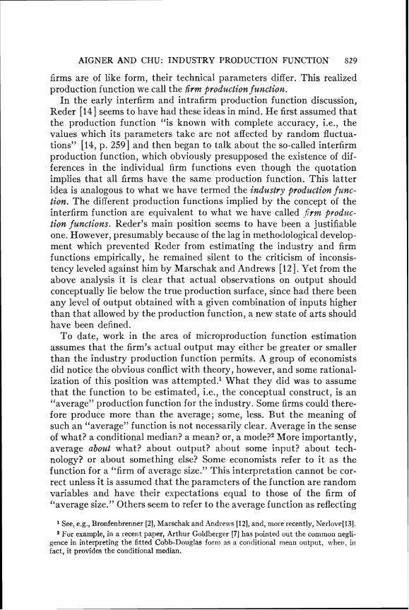
firms are of like form, their technical parameters differ. This realized production function we call the firm production function.

In the early interfirm and intrafirm production function discussion, Reder [14] seems to have had these ideas in mind. He first assumed that the production function '(is known with complete accuracy, i.e., the values which its parameters take are not affected by random fluctua- tions" 114, p. 2.591 and then began to talk about the so-called interfirm production function, which obviously presupposed the existence of dif- ferences in the individual firm functions even though the quotation implies that all firms have the same production function. This latter idea is analogous to what we have termed the industry production func- tion. The different production functions implied by the concept of the interfirm function are equivalent to what we have called -6rm ~ Y O ~ Z L C - tion functions. Reder's main position seems to have been a justifiable one. However, presumably because of the lag in methodological develop- ment which prevented Reder from estimating the industry and firm functions empirically, he remained silent to the criticism of inconsis- tency leveled against him by Marschak and Andrews 1121. Yet from the above analysis i t is clear that actual observations on output should conceptually lie below the true production surface, since had there been any level of output obtained with a given combination of inputs higher than that allowed by the production function, a new state of arts should have been defined.

To date, work in the area of microproduction function estimation assumes that the firm's actual output may either be greater or smaller than the industry production function permits. A group of economists did notice the obvious conflict with theory, however, and some rational- ization of this position was attempted.' What they did was to assume that the function to be estimated, i.e., the conceptual construct, is an "average" production function for the industry. Some firms could there- fore produce more than the average; some, less. But the meaning of such an "average" function is not necessarily clear. Average in the sense of what? a conditional median? a mean? or, a mode?2 More importantly, average about what? about output? about some input? about tech- nology? or about something else? Some economists refer to it as the function for a "firm of average size." This interpretation cannot be cor- rect unless i t is assumed that the parameters of the function are random variables and have their expectations equal to those of the firm of "average size." Others seem to refer to the average function as reflecting

1 See, e.g., Bronfenbrenner [2], Marschak and Xndren s [12], and, more recently, Nerlove[l3]. 2 For example, in a recent paper, Arthur Goldberger [7] has pointed out the common negli-

gence in interpreting the fitted Cobb-Douglas form as a co~lditiorlal mean output, nvhe11, in fact, it provides the conditional median.

some sort of "average technology." But it would be infeasible to assuine that a firm which possesses "average technology" with respect to cap- ital also has an "average technology" with respect to labor. Such a coincidence is even less likely when factors are treated in more definitive categories.

Another appealing interpretation is that "true" productive capacity only makes sense as an output level which can be sustained. The "aver- age" production function, devoid of random fluctuations due to '(lucky" coincidences of good weather, sunspots, etc., and "unlucky" ones as well, is thus promoted as the iunction of sustained output. But the no- tion of sustained output has long-run overtones which tend to invalidate this argument for the average function in a short-run context. Produc- tion processes which depend on uncontrollables like weather as explicit inputs (or catalysts) may be of a different conceptual nature than those of industry, for example, and to the extent that they exist (as in some forms of agricultural production) the frontier concept is unacceptable, but o d y because it assumes inputs to bc "variable" in the short run in the sense that the firm may control them.

From a more practical standpoint, i f , for example, we wish to esti- mate how much output on the average, could be obtained for a firm in the industry with a certain set of inputs, then the "average" concept would obviously be the correct one to employ. Another very important use of the average function which previously has been overlooked is that in some cases we can approximate the industry's aggregate produc- tion function when aggregate data cannot be obtained but data a t the iirm level are available; or, we can approximate an "average" firm pro- duction function when ure have data only on industry aggregates. The latter point is especially important because in practice data a t the firm level are usually not available. Hildebrancl and Liu's [9] belief that ob- servations for some "representative establishments" could be used to estimate 'L7.S. manufacturing production functions is consistent with the first part of the above statement.

Despite these uses for the "average" production function, use of the frontier function is appropriate in order to ascertain the maximum pro- ductive capacity of an industry (for purposes of planning, for example), of measuring the potential output of an economy, etc. Along these same lines, M. J. Farrell [ S ] [6] defined an "efficient production func- tion" which reseml~les our industry function, and devised an ingenious way of estimating this efficient production iunction through constructing isorlunnts. The difficulty with Farrell's method, however, is that it is not general enough. Many types of production cannot be characterized within his motlels. For esample, it is not possihle to estimate a produc-

AIGNER AND CHU: INDUSTRY PRODUCTION FUNCTLON 831

tion function with his method which conforms to the Law of t'ariable Proportions.

In the following section we attempt to indicate how familiar mathe- matical programming methods may be used in some cases where Far- rell's method would fail to obtain the required production surface. I n terms of the generality of approach, while we can alleviate the inherent difficulties of assuming something in advance about the shape of the e~pans ion path, our methods apply only to single output situations.

11. I'rograrnmilzg Methodology

T o begin, let us consider only the effects of random shocks on the production process; all differences in technical efficiency are subsumed within the disturbance term. Errors of measurement in all variables are also assumed negligible. For simplicity we take a one-output, two-input Cohb-T)ouglus model over firms.

with xo = output

xl, x2 = inputs

ZL = randoin shock

A , a:, p = parameters

Our problem is to obtain an estimated function

such that A ' ' .?a

(3.3) Azlxs > xo If we take logarithms of both sides of (3.1) and rewrite equations

(3.2) and (3.3) compactly in matrix notation, we have:

(3.4) Xo = XC + e

(3.5) -YC 2 -Yo,

where -Yo= log xo, .Y1 = log yl, 3-2 = log .Y,,

X = 11 x1x2] c = [.4 a: p]'

e = vector of measured residuals

One way to approach the estimation problems imposed by equations (3.4) and (3.5) is to minimize the sum of squared residuals (e'e) subject

832 T H E A M E R I C A N ECONOMIC R E V I E W

to (3 S), in which case we formulate the prol~lem as follows, in its form for the general linear production model (positive coefficients on inputs) :

To find the positive vector C3that minimizes the quadratic function

subject to:

X.uC 2 xo, (3 6) poses a typical ciuadratic programming proljlem and may be solvc.tl by Wolfe's algorithm [16].

Since the shocks lie only on one side of the industry production frontier, we may also treat the estimation problem easily within the framework of linear programming. In other words, we may minimize the sum of residuals, as a linear loss function, rather than the sum of squared residuals. The problem may then be written as follows:

To minimize

subject to:

I t is to be noted that for some purposes the linear programming esti- mator may be superior to the quadratic programming estimator since the criterion function is less influenced by extreme values. However, the quadratic programming method provides a convenient treatment when the simultaneous equation model is considered, as we shall see below.

Pu'ext, let us attempt to introduce technical efficiency into the model in such a fashion as to make the identification of individual firm func- tions possible within the context of the industry production function. One way to treat interfirm differences in technical efficiency is to regard them as a part of the disturbance term, as we have above, following R4arschak and Andrews [12]. Another approach is adopted by Hilde- brand and Liu [9] (hereafter referred to as H-L).These authors attempt to separate the effects of technical efficiency from shocks on theoretical grounds, in an effort to allow only the shocks to influence estimates. The advantage of their method is that (1) if the theoretical specification is correct, then unbiased estimates may be ~ b t a i n e d , ~ and (2) individual

3 Here we would allow the constant term to be of either sign by redefining X as X = [- 1 1 XI Xz], and C as C= [A!A2 a 81'. Then the algorithm is free to select A , or A2 (both positive). If A , is chosen (A2=0), the constant term is negative.

Under the assumption E (log u) =0. In a review of the H-L work McFadden [ l l]demon-strates that their empirical specification is incorrect, but that corrections to recover estimates of model structural parameters are available.

AIGNER AND CHU: INDUSTRY PRODUCTION FUNCTION 833

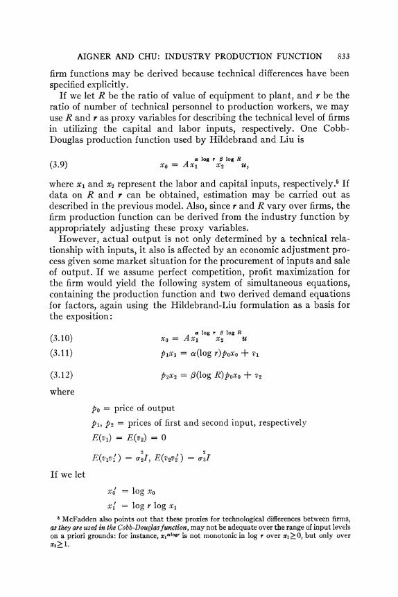
firm functions may be derived because technical differences have been specified explicitly.

If we let R be the ratio of value of equipment to plant, and r be the ratio of number of technical personnel to production workers, we may use R and r as proxy variables for describing the technical level of firms in utilizing the capital and labor inputs, respectively. One Cobb-Douglas production function used by I-Iildebrand and Liu is

a log r 6 log R -210 = A x l x2 U,

where xl and xz represent the labor and capital inputs, respectively."Ii data on R and r can be obtained, estimation may be carried out as described in the previous model. Also, since r and R vary over firms, the firm production function can be derived from the industry function by appropriately adjusting these proxy variables.

However, actual output is not only determined by a technical rela- tionship with inputs, i t also is affected by an economic adjustment pro- cess given some market situation for the procurement of inputs and sale of output. If we assume perfect competition, profit maximization for the firm would yield the following system of simultaneous equations, containing the production function and two derived demand equations for factors, again using the Hildebrand-Liu formulation as a basis for the exposition:

a log r 0 log Rx o = A x l ~2 u

where

po = price of output

pl , p2 = prices of first and second input, respectively

E(zll) = E(a2)= 0

If we let

.Yo' = log x0

x: = log r log xl

McFaddcn also points out that these proxies for technological differences between firms, as they are used in the Cobb-Douglasfunction,may not be adequate over the range of input levels on a priori grounds: for instance, x ~ a ' m ~is not monotonic in log r over 2120,but only over 2121.

834 THE AMERICAN ECONOMIC REVIEW

x i = log R log xz

ZI = (log rlpoxo

z:! = (log R)poxo

y1 = P l X l

A' = log A

11' = log u, with E(uul) = all

1' = number of observations

then equations (3.10)-(3.12) can be rewritten as:

(3.13) rv = zc + L',

For our purposes the simultaneous setting presents the additional problem of specifying $=EUU1, the variance-covariance matrix of disturbances, for use in constructing the appropriate quadratic loss function. In Zellner's work [17], for example, the Aitken generalized estimator is used for efficiency purposes. This specification, of a full $ matrix, has no known efiiciency properties under the restrictions we impose. Considering the nature of the disturbance u1,E [(zb') (u')'] =a121 has no particular significance for the loss function and also cannot, ap- parently, be estimated from sample data without specifying E(ut) . Moreover, one can quite reasonably argue for independence of the in- puts with output (or value added) in production models of this sort, so that the production functicn may be considered alone for purposes of estiniatio~l.';

111 light of this disc^:. .:on, if a simultaneous determination of coef- ricients is pursued $ must be specified in order to produce the quadratic loss function. Two alternatives seem plausible, but on intuitive grounds only: $= I (where I is 3TX3T) , and

Cf. Zellner, el al. 118, p. 7871. The Zellner paper considers production as stochastic a priori (as contrasted to our deterministic specification), but the key point is specification indepen- (lent: that the "effect of the disturbance on output cannot be known until efter the pre- \elected quantities of inputs have heen employed in production."

AlGNISR A S D ('HU: INDUSTRY PKO1)LC'l'ION FUN("1 ION 835

where k is an arbitrary weighting factor. With S a sample estimate of $ (or S= I ) , our estimation problem is:

To minimize

(3.14) C'U = (TV - z~) 's- ' (Tv- zC)

subject to

,As with (3.6), (3.14) should be viewed as being specified for a general linear system of equations.

111.An Exanzple of Use

T o illustrate the use of the programming methods, some empirical results are given here. The production function is version I11 in Hilde- brand and Liu [9; cf., p. 651, as applied to the primary metals industry.' The complete model in their notation is as follows:

(4.1) log V = log A + bo log L + eo log R-l log K-l + log u,

the production function, and

(4.2) log L = X log B + (1 - X ) log LP1+ (1 - m)X log 'I; - (1 - g ) X log TV - X log z

the labor demand f ~ n c t i o n . ~ Three versions of the programming method are used to produce esti-

mates of the coefficients in (4.1) : linear programming (LP) on (4.1), qua- dratic programming-single equation (QP1) on (4. I), and quadratic programming-simultaneous equation (QP2) on the two equation^.^ The results from such application, together with estimates derived from single equation least squares (1SLS) and two-stage least squares (2SLS) are tabulated below. The data used were for 1957-58, as it was not possible to reproduce perfectly the H-L data for 1956-57. The original H-L results are included in parentheses.

The table is presented in terms of H-L's original empirical work. However, McFadden7s criticism that H-L ignored the effects of inter- mediate good input and the output demand structure on bo and eo directs us to modify our procedures for computing the last four columns

II-L's data are state aggregates. \Ve use this e~ample for illustrative purposes primarily and ignore the obvious problems of specification and interpretation of the aggregation pro- cess on a framework developed for microdata.

L is labor, K-1 is the lagged (one year) value of capital, I; is value added for output, and W is the wage rate; z is a random term and X is specified as describing the speed of adjust- ment of the actual demand for labor to its optimal (profit maximizing) value,

9 In the QP2 results S was taken to be an identity matriu.

836 THE AMERICAN ECONOMIC REVIEW

from bo and eo. We will not, for purposes of this example, recompute all the relevant quantities. However, as an indication of changes in them, corrected estimates for the 2SLS row are: h=4.13, MPPL=1.005, capital-output elasticity = .02 1, and technology-output elasticity = .084. In general McFadden's results suggest that H-L's estimates of the scale factor for the two-digit industries considered are high. The con- clusion which follows (as contrasted to H-L's) is that no evidence is present which would indicate other than constant returns to scale in these manufacturing industries.

Reviewing the tabled results, the labor-output elasticity (bo) is highest for QP1 (1.071) and lowest for QP2 (.822). I t seems that the estimates from all five versions are plausible. The marginal physical product of labor per dollar of wage costs (MPPL) is again highest for QP1 (1.822) and lowest for QP2 (1.399). Following Hildebrand and Liu, the marginal revenue product of labor ($) is specified a t 0.8, which leads to derived estimates of the demand elasticity for output ( h ) :(h) is

-- .-- -

bo (Labor-Output

Elasticity)

eo (Output Demand

Elasticity)

Capital-Output

Elasticityb

Technology-Output

Elasticityb

lSLS .908 .0333 2.072 (11 IA. l ) (.988) (.0343)d (1 .886) 2SLS .917 ,0321 2.053 (111.A.2)0 (1.000) (.0326)d (1 .865) L P .873 .003 1 2.168 QP 1 QP2

1.071 .822

.0269

.0219 1.783 2.336

Marginal revenue product of labor per dollar of wage cost (6)assumed at 0.8. b 111R(~,, used for LP, QP1, QP2; 1nX for lSLS, 2SLS.

H-L's designation, cf. [9, p. 931. H-L's results are reported in terms of common log transformations, while we have used

the natural system. The base used is immaterial (so long as it is consistently used) in ob- taining the coefficient b ~ ,but the capital coefficient is affected by the base of the logarithms used. The translation is simple: for the equation fitted in common logarithms, the counter- part of the coefficient e~ if data is transformed by natural logs is eo'=eo.log ,,(2.718282)= ,434294 eo. Hildebrand and Liu are apparently consistent in their use of common logarithms for the empirical results, but overlooli the above scaling problem elsewhere (although it does not seem to cause any invalidation of results). For example [9, p. 50, footnote 81 there is the following:

d eo -(eo log R) = -dR R

If log R is a common logarithm, as they use in the empirical work. then

AIGNER AND CHU: INDUSTRY PRODUCTION FUNCTION 837

largest for QP2 (2.336) and smallest for QP1 (1.783). In view of the nature of this industry, these (indeed, all) values appear to be high, which suggests a smaller value of 4 should be used.1°

The significant difference between programming and regression re-sults appears in the capital coefficient and derivatives of it. The cap- ital-output elasticities for LP, QP1, and QP2 are respectively .0132, .1148, and 0.935, while those for one- and two-stage least squares are .I278 and .1232. The technology-output elasticity for L P is .0165; for QP1 and QP2, .I441 and .1173, respectively; for 1SLS and 2SLS, .5115 and .493 1.

Using the proxy variable R as an indicator of technological efficiency within the firms of the primary metals industry, our industry produc- tion function (from QP2) would be given by

(4.3) In V = 23221 In L + .0219.4.2673 In K-1 + constant

= A221 In L + .0935 In K-l + constant

where the maximum value for In R (for the state of Louisiana) is in- serted into the general form (4.1). This function would provide the maximum possible output (value added) from the labor and capital in- puts given the state of the arts in the industry. Clearly, any individual function (in this case, for a state) may be obtained by substituting the attained value of In R into (4.3).

Without an attempt to identify technological differences among firms explicitly, as with the proxy variables r and R, we still may, of course, obtain the industry production function in a simultaneous equation setting. However, individual firm (micro) functions may not be concomitantly estimated.

IV. Final Refnarks

A viable distinction between the average and frontier functions as predictors of capacity (and this is not a t all intended to give ground in the theoretical conflict) derives from a probability interpretation of al- ternative forecasts. On the one hand, the frontier function forecasts an "unlikely" event (output level), whereas the probability attached to t he output level given by the average function is higher. X fitted Cobb- Douglas function provides the conditional mec!ian output. So 50 per cent of firm outputs for a selected input combination should lie above that output predicted by the fitted Cobb-Douglas function. Of course, these remarks hold in the short run only: The frontier function under a fixed technology gives that output which, in the short run, only a few firms at most can produce for any given input combination (neglecting

10 The McFadden work suggests that even a wider discrepancy exists in adjusting 4 so the demand elasticity becomes more "reasonable."

838 THE AMERlCAN ECONOMIC REVIEW

scale differences). Allowing a longer run, as implied by the sustained output idea, but still assuming a fixed technology, more firms presum- ably become able to produce a t the maximum level; under this circum- stance, therefore, the frontier function should be the relatively better capacity predictor.

Finally, we have attempted to interpret the traditional theory strictly, in that the frontier we construct is truly a surface of maximum points. Under a different goal one may pursue less than 100 per cent frontiers using the chance-constrained programming ideas of Charnes- Cooper [3], where (3.3) would be translated into a probability state- ment, P r ( ~ x l k x , ~ > x ~ )with T a specified minimum probahiiity with ???, which the statement is to hold.

REFERENCES

1. V. ASHARAND T. D. WALLACE, "A Sanlpling Study of the Minimunl Absolute Deviations Estimator," Operations Resecl.1-ti z , Sept.-Oct. 1963, 11,7-17-58.

2. M. RRONFENBRENNER, Functions:' L P r ~ d ~ ~ t i ~ n Cobb-Douglas, Inter-Firm, Intra-Firm," Econometrica, Jan. 194-1. 12, 35--44.

2a. SUNE CARLSON, Prodzhction. Kew Yo]-B A Sfzhdy on the Pure Theory of 1956.

3. A. CHARNESAND W. \V. COOPER, "Deterministic Equivalents for Optimizing and Satisficing Under Chance Constraints," Operations Re- search, Jan.-Feb. 1963, 1 8 39.

4. G. DANTZIG~ N DA. ORDKN,"Di~itlity Theorems," RAND Report R. M. 1265.

5. M. J. FARRELL,((The Aleasurenient of Productive Efficiency," Jour. Royal Stat. Soc., Ser. A, 1957, 120, Pt. 3, 253-81.

6. --- '(Estimating Efficient Production Tinder , AND M. FIELDHOUSE, Increasing Returns to Scale," Jour. Royal Stat. Soc., Ser. -4, 1962, 125, Pt. 2, 252-67.

7. A. GOLDBERGER, the Interpretation of Cobb-"On and Estimation Douglas Functions," Econometrica, forthcoming.

8. J. M. HENDERSONAND R. QUANDT,M ~ C Y O C C O ~ Z O ~ ~ CTheory. New Work 1958.

9. G. HILDEBRAND in theAND T. I,Iu,ManzCfactnring Producfion F~~ncfio~zs United Stafes, 1957. 1thac.z 1905.

10. S.K ~ R L I N ,Aiathevzutical Metlfods and Theory in Gaines, Programt~zing, and Eco:~onzics, Vol. I , Iieading. Mass., 1959.

11. D. MCFADDEN,"Review of I-Iildebrand and I,ia," .l m. Stat.JOLLY. Assoc., June 1967, 62, 295-309.

12. J. MARSCH~K,4 N D IT. ANDREWS,"Random Simultaneous Equations and the Theory of the Production Fiulction," Economelrica, July-Oct. 5943, 12, 14.3-205.

13. MARCKFRLOVE, ofEstinzntion aud Identijca~ion Cobb-Douglas Produc- tion Functions. Chicago 1965.

AIGNER AXD CNU: INDUSTRY PRODUCII'ION FUNCTION 639

14. REDLR, ill. \v., 'LA\ll,111crnative Interpretation of the Cobb-L)ouglas Produ~t ion bunction," Ecotzo~netrica, Oct. 1953, 11,2.59-64.

15. T. Txsxlr.ura, AND G. JUDGE,"A Method for Handling Inequality Restrictions in Regression Analysis," J0167. Anz. Stat. Assoc., hlarch 1966, 61, 166-81.

10. 1'. i \ ' o i , b r , ','I'he Simplex Methotl for Qu:~d~, l t icl'rograninlirlg," l < l : ' ~ o r l o ~ i ~ r l r ~ ~ c r ,July 1959, 27, 383-98.

17. A. ZEI I N C K , "An Efficient Llethod of E:stim~ting Seelnirigly Unrelated Regressions and Tests for Aggregation Bias," JOZLY.Am. Stat. Assoc., June 1962, 57,348-68.

18. ---, J. KVEXTAAND J. D R ~ Z E ,"Specification and Estimation of Cohb-Douglas Productioa Function Models," Eco~zometrica, Oct. 1966, 34, 784-95.

You have printed the following article:

On Estimating the Industry Production FunctionD. J. Aigner; S. F. ChuThe American Economic Review, Vol. 58, No. 4. (Sep., 1968), pp. 826-839.Stable URL:

http://links.jstor.org/sici?sici=0002-8282%28196809%2958%3A4%3C826%3AOETIPF%3E2.0.CO%3B2-R

This article references the following linked citations. If you are trying to access articles from anoff-campus location, you may be required to first logon via your library web site to access JSTOR. Pleasevisit your library's website or contact a librarian to learn about options for remote access to JSTOR.

[Footnotes]

1 Production Functions: Cobb-Douglas, Interfirm, IntrafirmM. BronfenbrennerEconometrica, Vol. 12, No. 1. (Jan., 1944), pp. 35-44.Stable URL:

http://links.jstor.org/sici?sici=0012-9682%28194401%2912%3A1%3C35%3APFCII%3E2.0.CO%3B2-P

1 Random Simultaneous Equations and the Theory of ProductionJacob Marschak; William H. Andrews, Jr.Econometrica, Vol. 12, No. 3/4. (Jul. - Oct., 1944), pp. 143-205.Stable URL:

http://links.jstor.org/sici?sici=0012-9682%28194407%2F10%2912%3A3%2F4%3C143%3ARSEATT%3E2.0.CO%3B2-O

6 Specification and Estimation of Cobb-Douglas Production Function ModelsA. Zellner; J. Kmenta; J. DrèzeEconometrica, Vol. 34, No. 4. (Oct., 1966), pp. 784-795.Stable URL:

http://links.jstor.org/sici?sici=0012-9682%28196610%2934%3A4%3C784%3ASAEOCP%3E2.0.CO%3B2-Y

References

http://www.jstor.org

LINKED CITATIONS- Page 1 of 3 -

NOTE: The reference numbering from the original has been maintained in this citation list.

1 A Sampling Study of Minimum Absolute Deviations EstimatorsV. G. Ashar; T. D. WallaceOperations Research, Vol. 11, No. 5. (Sep. - Oct., 1963), pp. 747-758.Stable URL:

http://links.jstor.org/sici?sici=0030-364X%28196309%2F10%2911%3A5%3C747%3AASSOMA%3E2.0.CO%3B2-J

2 Production Functions: Cobb-Douglas, Interfirm, IntrafirmM. BronfenbrennerEconometrica, Vol. 12, No. 1. (Jan., 1944), pp. 35-44.Stable URL:

http://links.jstor.org/sici?sici=0012-9682%28194401%2912%3A1%3C35%3APFCII%3E2.0.CO%3B2-P

3 Deterministic Equivalents for Optimizing and Satisficing under Chance ConstraintsA. Charnes; W. W. CooperOperations Research, Vol. 11, No. 1. (Jan. - Feb., 1963), pp. 18-39.Stable URL:

http://links.jstor.org/sici?sici=0030-364X%28196301%2F02%2911%3A1%3C18%3ADEFOAS%3E2.0.CO%3B2-X

12 Random Simultaneous Equations and the Theory of ProductionJacob Marschak; William H. Andrews, Jr.Econometrica, Vol. 12, No. 3/4. (Jul. - Oct., 1944), pp. 143-205.Stable URL:

http://links.jstor.org/sici?sici=0012-9682%28194407%2F10%2912%3A3%2F4%3C143%3ARSEATT%3E2.0.CO%3B2-O

14 An Alternative Interpretation of the Cobb-Douglas FunctionM. W. RederEconometrica, Vol. 11, No. 3/4. (Jul. - Oct., 1943), pp. 259-264.Stable URL:

http://links.jstor.org/sici?sici=0012-9682%28194307%2F10%2911%3A3%2F4%3C259%3AAAIOTC%3E2.0.CO%3B2-I

16 The Simplex Method for Quadratic ProgrammingPhilip WolfeEconometrica, Vol. 27, No. 3. (Jul., 1959), pp. 382-398.Stable URL:

http://links.jstor.org/sici?sici=0012-9682%28195907%2927%3A3%3C382%3ATSMFQP%3E2.0.CO%3B2-0

http://www.jstor.org

LINKED CITATIONS- Page 2 of 3 -

NOTE: The reference numbering from the original has been maintained in this citation list.

18 Specification and Estimation of Cobb-Douglas Production Function ModelsA. Zellner; J. Kmenta; J. DrèzeEconometrica, Vol. 34, No. 4. (Oct., 1966), pp. 784-795.Stable URL:

http://links.jstor.org/sici?sici=0012-9682%28196610%2934%3A4%3C784%3ASAEOCP%3E2.0.CO%3B2-Y

http://www.jstor.org

LINKED CITATIONS- Page 3 of 3 -

NOTE: The reference numbering from the original has been maintained in this citation list.