on computing upper limits to source intensities
TRANSCRIPT
The Astrophysical Journal, 719:900–914, 2010 August 10 doi:10.1088/0004-637X/719/1/900C© 2010. The American Astronomical Society. All rights reserved. Printed in the U.S.A.
ON COMPUTING UPPER LIMITS TO SOURCE INTENSITIES
Vinay L. Kashyap1, David A. van Dyk
2, Alanna Connors
3, Peter E. Freeman
4, Aneta Siemiginowska
1, Jin Xu
2,
and Andreas Zezas5
1 Smithsonian Astrophysical Observatory, 60 Garden Street, Cambridge, MA 02138, USA; [email protected], [email protected] Department of Statistics, University of California, Irvine, CA 92697-1250, USA; [email protected], [email protected]
3 Eureka Scientific, 2452 Delmer Street, Suite 100, Oakland, CA 94602-3017, USA; [email protected] Department of Statistics, Carnegie Mellon University, 5000 Forbes Avenue, Pittsburgh, PA 15213, USA; [email protected]
5 Physics Department, University of Crete, P.O. Box 2208, GR-710 03, Heraklion, Crete, Greece; [email protected] 2010 February 4; accepted 2010 June 22; published 2010 July 23
ABSTRACT
A common problem in astrophysics is determining how bright a source could be and still not be detected inan observation. Despite the simplicity with which the problem can be stated, the solution involves complicatedstatistical issues that require careful analysis. In contrast to the more familiar confidence bound, this concept hasnever been formally analyzed, leading to a great variety of often ad hoc solutions. Here we formulate and describethe problem in a self-consistent manner. Detection significance is usually defined by the acceptable proportionof false positives (background fluctuations that are claimed as detections, or Type I error), and we invoke thecomplementary concept of false negatives (real sources that go undetected, or Type II error), based on the statisticalpower of a test, to compute an upper limit to the detectable source intensity. To determine the minimum intensitythat a source must have for it to be detected, we first define a detection threshold and then compute the probabilitiesof detecting sources of various intensities at the given threshold. The intensity that corresponds to the specifiedType II error probability defines that minimum intensity and is identified as the upper limit. Thus, an upper limitis a characteristic of the detection procedure rather than the strength of any particular source. It should not beconfused with confidence intervals or other estimates of source intensity. This is particularly important given thelarge number of catalogs that are being generated from increasingly sensitive surveys. We discuss, with examples,the differences between these upper limits and confidence bounds. Both measures are useful quantities that shouldbe reported in order to extract the most science from catalogs, though they answer different statistical questions:an upper bound describes an inference range on the source intensity, while an upper limit calibrates the detectionprocess. We provide a recipe for computing upper limits that applies to all detection algorithms.
Key words: methods: data analysis – methods: statistical
1. INTRODUCTION
When a known or suspected source remains undetected ata prescribed statistical significance during an observation, itis customary to report the upper limit on its intensity. Thislimit is usually taken to mean the largest intrinsic intensitythat a nominal source can have with an appreciable chanceof going undetected. Or equivalently, it is the smallest intrinsicintensity the source could have before its detection probabilityfalls below a certain threshold. We emphasize that the upperlimit is not meant to be an estimate or even a bound onthe intensity of the source, but rather it is a quantificationof the power of the detection procedure to detect weak sources.Thus, it is a measure that characterizes the detection process.The endpoints of the confidence interval, by contrast, provideranges of possible values for the source intensity rather thanquantify the sensitivity of the procedure. While the concept ofupper limits has generally been well understood by astronomersas a form of censoring (Isobe et al. 1986) with an intrinsicconnection to the detectability of a source (Avni et al. 1980),there has not been a statistically meaningful description thatencapsulates its reliance on detectability as well as statisticalsignificance.
Moreover, while the term “upper limit” has been traditionallyused in this manner, it has also been used in cases where aformal detection process is not applied (e.g., when a sourceis known to exist at a given location because of a detection
made in some other wavelength). In such cases, the upper edgeof the confidence interval is derived and noted as the upperlimit, regardless of the detectability of that source. In orderto prevent confusion, we shall henceforth refer to the upperedge of a confidence interval as the “upper bound.” Despitethe intrinsic differences, numerous studies have described thecomputation of the upper bound as a proxy for the upper limitin increasingly sophisticated ways. The parameter confidenceinterval is statistically well understood and is in common use.Kraft et al. (1991) and Marshall (1992), for example, appliedPoisson Bayesian-likelihood analysis to X-ray counts data todetermine the credible range and thus set an upper bound on thesource intensity. Feldman & Cousins (1998) recognized that theclassical confidence interval at a given significance is not unique,and devised a scheme to determine intervals by comparingthe likelihoods of obtaining the observed number of countswith the maximum likelihood estimate of the intensity anda nominal intensity; this procedure produces unique intervalswhere the lower edge overlaps with zero when there are veryfew counts, and the upper edge stands as a proxy for anupper limit. Variations in the background were incorporatedvia a sophisticated Bayesian analysis by Weisskopf et al.(2007).
The similarity of nomenclature between upper limits andupper bounds has led to considerable confusion in the literatureon the nature of upper limits, how to compute them, and whattype of data to use to do so. Many techniques have been used
900
No. 1, 2010 COMPUTING UPPER LIMITS TO SOURCE INTENSITIES 901
to determine upper limits. It is not feasible to list all of these,6
but for the sake of definiteness, we list a few methods culledfrom the literature: the techniques range from using the root-mean-square deviations in the background to set the upper limit(Gilman et al. 1986; Ayres 1999, 2004; Perez-Torres et al.2009), adopting the source detection threshold as the upperlimit (Damiani et al. 1997; Erdeve et al. 2009; Rudnick &Lemmerman 2009), computing the flux required to change afit statistic value by a significant amount (Loewenstein et al.2009), computing the p-value for the significance of a putativedetection in the presence of background (Pease et al. 2006;Carrera et al. 2007), and identifying the upper limit with theparameter confidence bound (Schlegel & Petre 1993; Hugheset al. 2007). Here, we seek to clarify these historically oftenused terms in a statistically rigorous way.
Our goal here is to illustrate the difference between upperlimits and upper bounds, and to develop a self-consistent de-scription for the former that can be used with all extant detec-tion techniques. Bounds and limits describe answers to differentstatistical questions, and usually both should be reported in de-tection problems. We seek to clarify their respective usage here.We set out the requisite definitions and statistical foundationsin Section 2. In Section 3, we discuss the critical role played bythe detection threshold in the definition of an upper limit andcompare upper limits with upper bounds of confidence intervals.In Sections 2 and 3, we use a simple Poisson detection problemas a running example to illustrate our methods. In Section 4, weapply them to a signal-to-noise detection problem. Finally, wesummarize in Section 5.
2. STATISTICAL BACKGROUND
Here we begin by describing our notation, and then discussthe nuances of the familiar concepts of confidence intervals,hypothesis testing, and statistical power. A glossary of thenotation used is given in Table 1.
2.1. Description of the Problem
Our study is carried out in the context of background-contaminated detection of point sources in photon counting de-tectors, as in X-ray astronomical data. We set up the problemfor the case of uncomplicated source detection (i.e., ignoringsource confusion, intrinsic background variations, and instru-mental effects such as vignetting, detector efficiency, PSF struc-ture, bad pixels, etc). However, the methodology we develop issufficiently general to apply in complex situations.
There is an important, subtle, and often overlooked distinctionbetween an upper limit and the upper bound of a confidenceinterval, and the primary goal of this paper is to illuminate thisdifference. The confidence interval is the result of inferenceon the source intensity, while the upper limit is a measureof the power of the detection process. We can precisely statethis difference in the context of an example. Suppose thatwe have a typical case of a source detection problem, wherecounts are collected in a region containing a putative or possiblesource and are compared with counts from a source-free region
6 An ADS query on astronomy abstracts, within the past year (excludingarXiv), containing “upper limit,” yields roughly two papers per day (759). Aquick survey shows this term used in several disparate ways: some are upperbounds of confidence regions, often convolved with physics information to getthe upper bound of a confidence region on (say) mass; others are clearly thetheoretical power of a suggested test; yet others use “upper limits” fromprevious work to obtain, e.g., line slopes.
Table 1Symbols and Notation
Symbol Description
nS Counts observed in source areanB Counts observed in background areaλS Source intensityλB Background intensityΛB Range in background intensity λB
τS Exposure timeτB Exposure time for the backgroundr Ratio of background to source areaS Statistic for hypothesis test
S�Detection threshold value of statistic S
n�S Detection threshold value of statistic nS
U Upper limitα The maximum probability of false detectionβ The probability of a detectionβmin The minimum probability of detection of a source with λS = UPr(.) Probability ofn ∼ f (.) Denoting that n is sampled from the distribution f (.)Poisson(λ) Poisson distribution with intensity λ
N (μ, σ ) Gaussian (i.e., normal) distribution with mean μ and variance σ 2
that defines the background. If the source counts exceed thethreshold for detection, the source is considered to be detected.This detection threshold is usually determined by limiting theprobability of a false detection. If the threshold were lower,there would be more false detections. Given this setup, we mightask how bright must a source be in order to ensure detection.Although statistically there are no guarantees, the upper limitis the minimum brightness that ensures a certain probabilityof detection. Critically, this value can be computed before thesource counts are observed. It is based on two probabilities,(1) the probability of a false detection which determines thedetection threshold and (2) the minimum probability that abright source is detected. Although the upper limit is primarilyof interest when the observed counts are less than the detectionthreshold, it does not depend on the observed counts. This is insharp contrast to a confidence interval for the source intensity,that is typically of the form “source intensity estimate plus orminus an error bar,” where the estimate and error bars dependdirectly on the observed source counts in the putative sourceregion. Of course, the functional form of the confidence intervalmay be more complicated than in this example, especially in lowcount settings, but any reasonable confidence interval dependson the source counts, unlike upper limits. The fact that upperlimits do not depend on the source counts while confidenceintervals do should not be viewed as an advantage of onequantity or the other. Rather it reflects their differing goals.Upper limits quantify the power of the detection procedureand confidence intervals describe likely values of the sourceintensity. These distinctions are highlighted with illustrativeexamples in Section 3.1.1.
To formalize discussion, suppose that a known source hasan intrinsic intensity in a given passband of λS and that thebackground intensity under the source is λB . Further supposethat the source is observed for a duration τS and that nS countsare collected, and similarly, a separate measurement of thebackground could be made over a duration τB and nB countsare collected. If the background counts are collected in an area
902 KASHYAP ET AL. Vol. 719
r times the source area,7 we can relate the observed counts tothe expected intensities,
nB |(λB, r, τB ) ∼ Poisson(rτBλB)
nS |(λS, λB, τS) ∼ Poisson(τS(λS + λB)
), (1)
in the background and source regions respectively, where nB andnS are independent. For simplicity, we begin by assuming thatλB is known.
2.2. Confidence and Credible Intervals
Confidence intervals give a set of values for the sourceintensity that are consistent with the observed data. They aretypically part of the inference problem for the source intensity.The basic strategy is to compute an interval of parametervalues so that on repeated observations a certain proportionof the intervals contain the true value of the parameter. It isin this “repeated-observation” sense that a classical confidenceinterval has a given probability of containing the true parameter.Bayesian credible intervals have a more direct probabilisticinterpretation. They are computed by deriving the posteriorprobability distribution of the source intensity parameter giventhe observed counts and finding an interval with nominalprobability of containing the true rate (see, e.g., Loredo 1992;van Dyk et al. 2001; Kashyap et al. 2008). In summary,confidence intervals are frequentist in nature meaning that theyare interpreted in terms of repeated observations of the source.Credible intervals, on the other hand, are Bayesian in naturemeaning that they represent an interval of a certain posterior (orother Bayesian) probability.
2.2.1. Confidence Intervals
From a frequentist point of view randomness stems onlyfrom data collection—it is the data, not the parameters thatare random. Often we use a 95% interval, but intervals may beat any level and we more generally refer to an L% confidenceinterval. Thus, the proper interpretation of a given interval is
L% of experiments (i.e., observations) with intervals com-puted in this way will result in intervals that contain thetrue value of the source intensity.
In frequentist terms, this means that in any given experimentone cannot know whether the true source intensity is containedin the interval but if the experiment is repeated a large numberof times, about L% of the resulting intervals will contain the truevalue. Strictly speaking, the more colloquial understanding thatthere is an L% chance that the “source intensity is contained inthe reported confidence interval,” is incorrect.
Put another way, a confidence interval for the source intensitygives values of λS that are plausible given the observed counts.Suppose that λB = 3 and that for each value of λS , we constructan interval I(λS) of possible values of the source counts thathas at least an L% chance: Pr(nS ∈ I(λS)|λS, λB, τS) � L%.
7 For clarity, we assume that the expected intensities are in units of counts perunit time and that the source and background counts are collected overpre-specified areas in an image. However, our analysis is not restricted to thisscenario. The nominal background-to-source area ratio r could includedifferences in exposure duration and instrument effective area. Furthermore,the nominal exposure duration could also incorporate effective area, e.g., tohave units [photons count−1 cm2 s], which implies that the expected intensityλS will have units [photons s−1 cm−2]. Regardless of the units of λS and λB ,the likelihood is determined by the Poisson distribution on the expected andobserved counts as in Equation (1).
Once the source count is observed and assuming λB is known,a confidence interval can be constructed as the set of values ofλS for which the observed count is contained in I(λS),
{λS : nS ∈ I(λS)} . (2)
In repeated observations, at least L% of intervals computed inthis way cover the true value of λS .
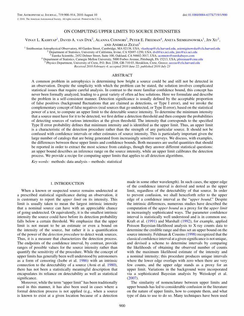
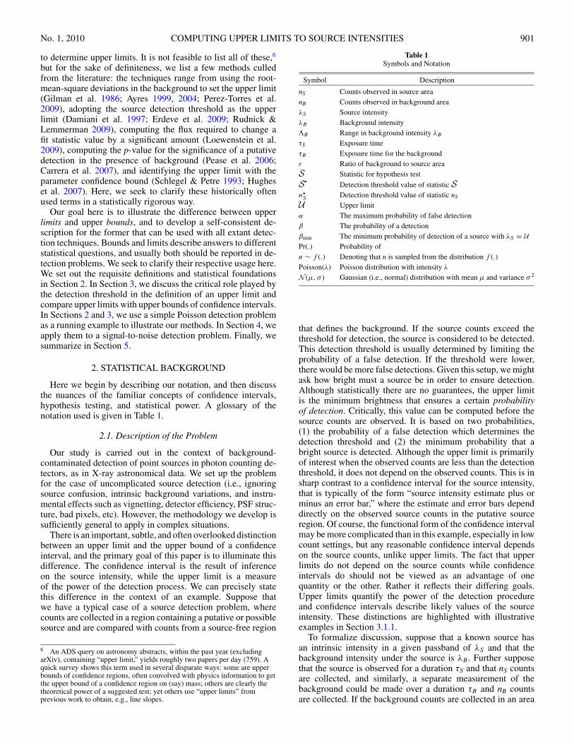
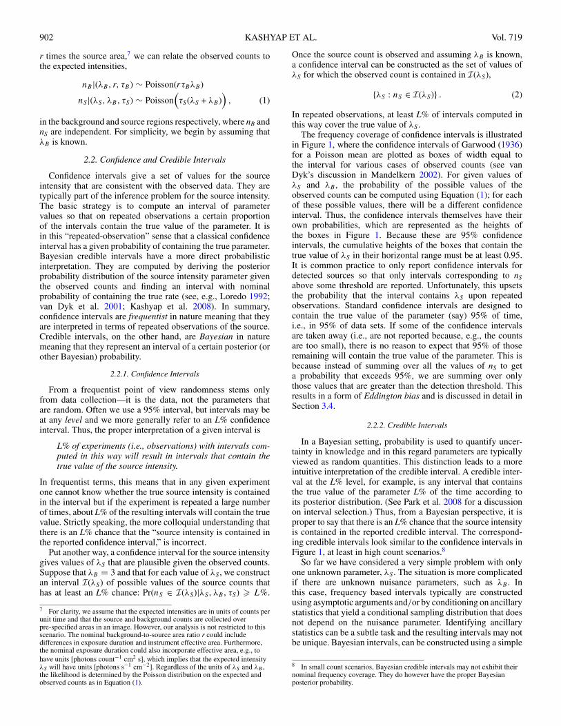
The frequency coverage of confidence intervals is illustratedin Figure 1, where the confidence intervals of Garwood (1936)for a Poisson mean are plotted as boxes of width equal tothe interval for various cases of observed counts (see vanDyk’s discussion in Mandelkern 2002). For given values ofλS and λB , the probability of the possible values of theobserved counts can be computed using Equation (1); for eachof these possible values, there will be a different confidenceinterval. Thus, the confidence intervals themselves have theirown probabilities, which are represented as the heights ofthe boxes in Figure 1. Because these are 95% confidenceintervals, the cumulative heights of the boxes that contain thetrue value of λS in their horizontal range must be at least 0.95.It is common practice to only report confidence intervals fordetected sources so that only intervals corresponding to nSabove some threshold are reported. Unfortunately, this upsetsthe probability that the interval contains λS upon repeatedobservations. Standard confidence intervals are designed tocontain the true value of the parameter (say) 95% of time,i.e., in 95% of data sets. If some of the confidence intervalsare taken away (i.e., are not reported because, e.g., the countsare too small), there is no reason to expect that 95% of thoseremaining will contain the true value of the parameter. This isbecause instead of summing over all the values of nS to geta probability that exceeds 95%, we are summing over onlythose values that are greater than the detection threshold. Thisresults in a form of Eddington bias and is discussed in detail inSection 3.4.
2.2.2. Credible Intervals
In a Bayesian setting, probability is used to quantify uncer-tainty in knowledge and in this regard parameters are typicallyviewed as random quantities. This distinction leads to a moreintuitive interpretation of the credible interval. A credible inter-val at the L% level, for example, is any interval that containsthe true value of the parameter L% of the time according toits posterior distribution. (See Park et al. 2008 for a discussionon interval selection.) Thus, from a Bayesian perspective, it isproper to say that there is an L% chance that the source intensityis contained in the reported credible interval. The correspond-ing credible intervals look similar to the confidence intervals inFigure 1, at least in high count scenarios.8
So far we have considered a very simple problem with onlyone unknown parameter, λS . The situation is more complicatedif there are unknown nuisance parameters, such as λB . Inthis case, frequency based intervals typically are constructedusing asymptotic arguments and/or by conditioning on ancillarystatistics that yield a conditional sampling distribution that doesnot depend on the nuisance parameter. Identifying ancillarystatistics can be a subtle task and the resulting intervals may notbe unique. Bayesian intervals, can be constructed using a simple
8 In small count scenarios, Bayesian credible intervals may not exhibit theirnominal frequency coverage. They do however have the proper Bayesianposterior probability.
No. 1, 2010 COMPUTING UPPER LIMITS TO SOURCE INTENSITIES 903
0 5 10 15 20 25
0.0
0.2
0.4
0.6
0.8
1.0
Cu
mu
lati
ve P
rob
abili
ty
nS = 0
nS = 1
nS = 2
nS = 3
nS = 4nS = 5nS > 5
λS = 1λB = 1
0 5 10 15 20 25
0.0
0.2
0.4
0.6
0.8
1.0
nS = 0nS = 1
nS = 2
nS = 3
nS = 4
nS = 5
nS = 6nS = 7
nS = 8 nS > 8
λS = 1λB = 3
0 5 10 15 20 25
0.0
0.2
0.4
0.6
0.8
1.0
nS < 2nS = 2
nS = 3
nS = 4
nS = 5
nS = 6
nS = 7
nS = 8nS = 9
nS = 10nS = 11nS > 11
λS = 1λB = 5
0 5 10 15 20 25
0.0
0.2
0.4
0.6
0.8
1.0
Cu
mu
lati
ve P
rob
abili
ty
nS = 0nS = 1
nS = 2
nS = 3
nS = 4
nS = 5
nS = 6nS = 7
nS = 8nS > 8
λS = 3λB = 1
0 5 10 15 20 25
0.0
0.2
0.4
0.6
0.8
1.0
nS < 2nS = 2
nS = 3
nS = 4
nS = 5
nS = 6
nS = 7
nS = 8nS = 9
nS = 10nS = 11...
λS = 3λB = 3
0 5 10 15 20 25
0.0
0.2
0.4
0.6
0.8
1.0
nS < 3nS = 3
nS = 4nS = 5
nS = 6
nS = 7
nS = 8
nS = 9
nS = 10nS = 11
nS = 12nS = 13
...
λS = 3λB = 5
0 5 10 15 20 25
0.0
0.2
0.4
0.6
0.8
1.0
λS
Cu
mu
lati
ve P
rob
abili
ty
nS < 2nS = 2
nS = 3
nS = 4
nS = 5
nS = 6
nS = 7
nS = 8nS = 9
nS = 10nS = 11...
λS = 5λB = 1
0 5 10 15 20 25
0.0
0.2
0.4
0.6
0.8
1.0
λS
...nS = 3nS = 4
nS = 5
nS = 6
nS = 7
nS = 8
nS = 9
nS = 10nS = 11
nS = 12nS = 13
...
λS = 5λB = 3
0 5 10 15 20 25
0.0
0.2
0.4
0.6
0.8
1.0
λS
...nS = 4nS = 5
nS = 6nS = 7
nS = 8
nS = 9
nS = 10
nS = 11
nS = 12nS = 13
nS = 14nS = 15
...
λS = 5λB = 5
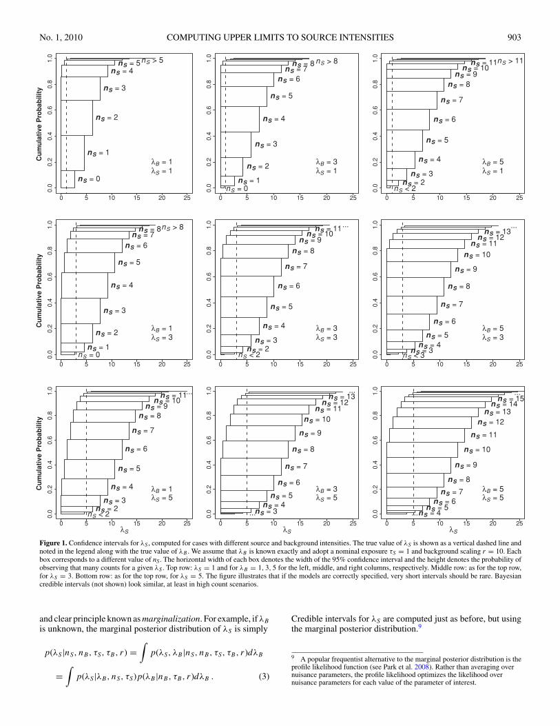
Figure 1. Confidence intervals for λS , computed for cases with different source and background intensities. The true value of λS is shown as a vertical dashed line andnoted in the legend along with the true value of λB . We assume that λB is known exactly and adopt a nominal exposure τS = 1 and background scaling r = 10. Eachbox corresponds to a different value of nS. The horizontal width of each box denotes the width of the 95% confidence interval and the height denotes the probability ofobserving that many counts for a given λS . Top row: λS = 1 and for λB = 1, 3, 5 for the left, middle, and right columns, respectively. Middle row: as for the top row,for λS = 3. Bottom row: as for the top row, for λS = 5. The figure illustrates that if the models are correctly specified, very short intervals should be rare. Bayesiancredible intervals (not shown) look similar, at least in high count scenarios.
and clear principle known as marginalization. For example, if λB
is unknown, the marginal posterior distribution of λS is simply
p(λS |nS, nB, τS, τB, r) =∫
p(λS, λB |nS, nB, τS, τB, r)dλB
=∫
p(λS |λB, nS, τS)p(λB |nB, τB, r)dλB . (3)
Credible intervals for λS are computed just as before, but usingthe marginal posterior distribution.9
9 A popular frequentist alternative to the marginal posterior distribution is theprofile likelihood function (see Park et al. 2008). Rather than averaging overnuisance parameters, the profile likelihood optimizes the likelihood overnuisance parameters for each value of the parameter of interest.
904 KASHYAP ET AL. Vol. 719
0 2 4 6 8 10 12 14
05
1015
20
λB
S*
α = 0.01α = 0.05α = 0.1
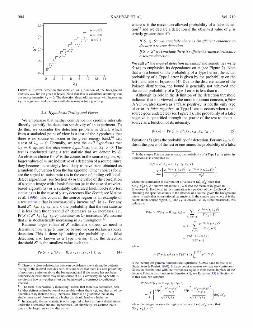
Figure 2. α-level detection threshold S� as a function of the backgroundintensity λB , for the given α levels. Note that this is calculated assuming thatthe source intensity λS = 0. The detection threshold increases with increasingλB for a given α, and increases with decreasing α for a given λB .
2.3. Hypothesis Testing and Power
We emphasize that neither confidence nor credible intervalsdirectly quantify the detection sensitivity of an experiment. Todo this, we consider the detection problem in detail, whichfrom a statistical point of view is a test of the hypothesis thatthere is no source emission in the given energy band,10 i.e.,a test of λS = 0. Formally, we test the null hypothesis thatλS = 0 against the alternative hypothesis that λS > 0. Thetest is conducted using a test statistic that we denote by S.An obvious choice for S is the counts in the source region, nS;larger values of nS are indicative of a detection of a source, sincethey become increasingly less likely to have been obtained asa random fluctuation from the background. Other choices for Sare the signal-to-noise ratio (as in the case of sliding-cell local-detect algorithms; see Section 4) or the value of the correlationof a counts image with a basis function (as in the case of wavelet-based algorithms) or a suitably calibrated likelihood-ratio teststatistic (as in the case of γ -ray detectors like Fermi; see Mattoxet al. 1996). The count in the source region is an example ofa test statistic that is stochastically increasing11 in λS . For anyfixed S�, λB , τS , τB , and r, the probability that the test statisticS is less than the threshold S� decreases as λS increases, i.e.,Pr(S � S�|λS, λB, τS, r) decreases as λS increases. We assumethat S is stochastically increasing in λS throughout.12
Because larger values of S indicate a source, we need todetermine how large S must be before we can declare a sourcedetection. This is done by limiting the probability of a falsedetection, also known as a Type I error. Thus, the detectionthreshold S� is the smallest value such that
Pr(S > S�|λS = 0, λB, τS, τB, r) � α, (4)
10 There is a close relationship between confidence intervals and hypothesistesting. If the interval includes zero, this indicates that there is a real possibilityof no source emission above the background and if the source has not beenotherwise detected there may be no source at all. Conversely, in Appendix Awe discuss how a hypothesis test can be inverted to construct a confidenceinterval.11 The term “stochastically increasing” means that there is a parameter (hereλS ) that defines a distribution of observable values (here nS), and that all of thequantiles of nS increase as λS increases. There is no guarantee that at anysingle instance of observation, a higher λS should lead to a higher nS.12 In principle, the test statistic is only required to have different distributionsunder the alternative and null hypotheses. For simplicity, we assume that ittends to be larger under the alternative.
where α is the maximum allowed probability of a false detec-tion13 and we declare a detection if the observed value of S isstrictly greater than S�:
If S � S� we conclude there is insufficient evidence todeclare a source detection.
IfS > S� we conclude there is sufficient evidence to declarea source detection.
We call S� the α-level detection threshold and sometimes writeS�(α) to emphasize its dependance on α (see Figure 2). Notethat α is a bound on the probability of a Type I error; the actualprobability of a Type I error is given by the probability on theleft-hand side of Equation (4). Due to the discrete nature of thePoisson distribution, the bound is generally not achieved andthe actual probability of a Type-I error is less than α.
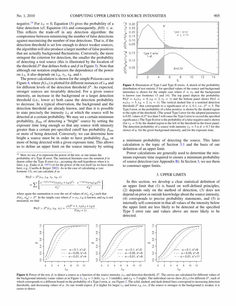
Although its role in the definition of the detection thresholdindicates that it is viewed as the more important concern, a falsedetection, also known as a “false positive,” is not the only typeof error. A false negative, or Type II error, occurs when a realsource goes undetected (see Figure 3). The probability of a falsenegative is quantified through the power of the test to detect asource as a function of its intensity,
β(λS) = Pr(S > S�|λS, λB, τS, τB, r) . (5)
Equation (5) gives the probability of a detection. For any λS > 0,this is the power of the test or one minus the probability of a false
13 In the simple Poisson counts case, the probability of a Type I error given inEquation (4) is computed as
Pr(S > S�|λS = 0, λB, τS, τB, r)
=∑ {
e−τSλB (τSλB )n′S
n′S !
· e−rτBλB (rτBλB )n′B
n′B !
},
where the summation is over the set of values of (n′S, n′
B ) such thatS(n′
S, n′B ) > S� and we substitute λS = 0 into the mean of nS given in
Equation (1). Each term in the summation is a product of the likelihood ofobtaining the specified counts in the absence of a source, given the backgroundintensity and other observational parameters. In the simple case where S is thecounts in the source region, nS, and λB is known (i.e., nB is not measured), thisreduces to
Pr(S > S�|λS = 0, λB, τS ) =∞∑
n′S=S�+1
e−τSλB (τSλB )n′S
Γ(n′S + 1)
= 1 −S�∑
n′S=0
e−τSλB (τSλB )n′S
Γ(n′S + 1)
= γ (S� + 1, τSλB )
Γ(S� + 1),
where
γ (S� + 1, τSλB ) = Γ(S� + 1)∫ τSλB
0e−t tnS dt
is the incomplete gamma function (see Equations (8.350.1) and (8.352.1) ofGradshteyn & Ryzhik 1980). In large count scenarios we may use continuousGaussian distributions with their variances equal to their means in place of thediscrete Poisson distributions in Equation (1); see Equation (13) in Section 4.In this case, we compute
Pr(S>S�|λS = 0, λB, τS, τB, r)
=∫ { exp
[− (n′
S−τSλB )2
τSλB
]√
2πτSλB
·exp
[− (n′
B−rτBλB )2
rτBλB
]√
2πrτBλB
}dn′
Sdn′B,
where the integral is over the region of values of (n′S, n′
B ) such thatS(n′
S, n′B ) > S�.
No. 1, 2010 COMPUTING UPPER LIMITS TO SOURCE INTENSITIES 905
negative.14 For λS = 0, Equation (5) gives the probability of afalse detection (cf. Equation (4)) and consequently, β(0) � α.This reflects the trade-off in any detection algorithm: thecompromise between minimizing the number of false detectionsagainst maximizing the number of true detections. That is, if thedetection threshold is set low enough to detect weaker sources,the algorithm will also produce a larger number of false positivesthat are actually background fluctuations. Conversely, the morestringent the criterion for detection, the smaller the probabilityof detecting a real source (this is illustrated by the location ofthe threshold S� that defines both α and β in Figure 3). Note thatalthough our notation emphasizes the dependence of the poweron λS , it also depends on λB , τS , τB , and r.
The power calculation is shown for the simple Poisson case inFigure 4, where β(λS) is plotted for different instances of λB andfor different levels of the detection threshold S�. As expected,stronger sources are invariably detected. For a given sourceintensity, an increase in the background or a larger detectionthreshold (i.e., lower α) both cause the detection probabilityto decrease. In a typical observation, the background and thedetection threshold are already known, and thus it is possibleto state precisely the intensity λS at which the source will bedetected at a certain probability. We may set a certain minimumprobability, βmin of detecting a “bright” source by setting theexposure time long enough so that any source with intensitygreater than a certain pre-specified cutoff has probability βminor more of being detected. Conversely, we can determine howbright a source must be in order to have probability βmin ormore of being detected with a given exposure time. This allowsus to define an upper limit on the source intensity by setting
14 Here we use β to represent the power of the test, or one minus theprobability of a Type II error. The statistical literature uses the notation β todenote either the Type II error (i.e., accepting the null hypothesis when it isfalse; e.g., Eadie et al. 1971) or for the power of the test itself (as we have donehere; e.g., Casella & Berger 2002). As in the case of calculating α (seefootnote 13), we can calculate β as
Pr(S > S�|λS, λB, τS, τB, r)
=∑{
e−τS (λS +λB )(τS (λS + λB ))n′S
n′S !
· e−rτBλB (rτBλB )n′B
n′B !
},
where again the summation is over the set of values of (n′S, n′
B ) such thatS(n′
S, n′B ) > S�. In the simple case where S = nS , λB is known, and nB is not
measured, we find
Pr(S > S�|λS, λB, τS ) = γ (S� + 1, τS (λS + λB ))
Γ(nS + 1).
Figure 3. Illustration of Type I and Type II errors. A sketch of the probabilitydistribution of test statistic S for specified values of the source and backgroundintensities is shown for the simple case where S ≡ nS and the backgroundis known (see footnotes 13 and 14). The top panel depicts the probabilityPr(S = nS |λS = 0, λB = 2, τS = 1) and the bottom panel shows Pr(S =nS |λS = 5, λB = 2, τS = 1). The vertical dashed line is a nominal detectionthreshold S� that corresponds to a significance of α � 0.1, i.e., S� = 5. TheType I error, or the probability of a false positive, is shown by the shaded regionto the right of the threshold. (The actual Type I error for the adopted parametersis 0.05; values of S� less than 5 will cause the Type I error to exceed the specifiedsignificance.) The Type II error is the probability of a false negative and is shown(for λS = 5) by the shaded region to the left of the threshold in the lower panel.The detection probability of a source with intensity λS = 5 is β = 0.7 for thischoice of α, for the given background intensity, and for the exposure time.
a minimum probability of detecting the source. This lattercalculation is the topic of Section 3.1 and the basis of ourdefinition of an upper limit.
Power calculations are generally used to determine the min-imum exposure time required to ensure a minimum probabilityof source detection (see Appendix B). In Section 3, we use themto construct upper limits.
3. UPPER LIMITS
In this section, we develop a clear statistical definition ofan upper limit that (1) is based on well-defined principles,(2) depends only on the method of detection, (3) does notdepend on prior or outside knowledge about the source intensity,(4) corresponds to precise probability statements, and (5) isinternally self-consistent in that all values of the intensity belowthe upper limit are less likely to be detected at the specifiedType I error rate and values above are more likely to bedetected.
0 2 4 6 8 10 12
0.0
0.2
0.4
0.6
0.8
1.0
λS
β
α = 0.1, s*=2α = 0.05, s*=3α = 0.01, s*=4
0 2 4 6 8 10 12
0.0
0.2
0.4
0.6
0.8
1.0
λS
β
α = 0.1, s*=5α = 0.05, s*=6α = 0.01, s*=8
0 2 4 6 8 10 12
0.0
0.2
0.4
0.6
0.8
1.0
λS
β
α = 0.1, s*=8α = 0.05, s*=9
α = 0.01, s*=11
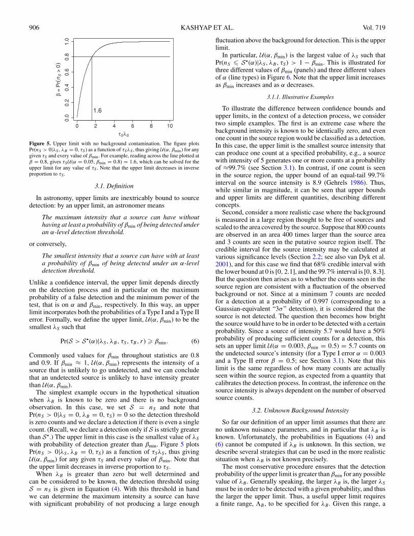
Figure 4. Power of the test, β, to detect a source as a function of the source intensity, λS , and detection threshold, S�. The curves are calculated for different values ofthe background intensity (same values as in Figure 1), λB = 1 (left), λB = 3 (middle), and λB = 5 (right). The individual curves show β(λS ) for different S�, each ofwhich corresponds to a different bound on the probability of a Type I error, α, see Figure 2. The solid, dashed, and dash-dotted lines correspond to increasing detectionthresholds, and decreasing values of α. As one would expect, β is higher for larger λS and lower λB , i.e., if the source is stronger or the background is weaker, it iseasier to detect.
906 KASHYAP ET AL. Vol. 719
0 2 4 6 8 10
0.0
0.2
0.4
0.6
0.8
1.0
τSλS
β =
Pr( n
S >
0)
1.6
Figure 5. Upper limit with no background contamination. The figure plotsPr(nS > 0|λS, λB = 0, τS ) as a function of τSλS , thus giving U(α, βmin) for anygiven τS and every value of βmin. For example, reading across the line plotted atβ = 0.8, gives τSU(α = 0.05, βmin = 0.8) = 1.6, which can be solved for theupper limit for any value of τS . Note that the upper limit decreases in inverseproportion to τS .
3.1. Definition
In astronomy, upper limits are inextricably bound to sourcedetection: by an upper limit, an astronomer means
The maximum intensity that a source can have withouthaving at least a probability of βmin of being detected underan α-level detection threshold.
or conversely,
The smallest intensity that a source can have with at leasta probability of βmin of being detected under an α-leveldetection threshold.
Unlike a confidence interval, the upper limit depends directlyon the detection process and in particular on the maximumprobability of a false detection and the minimum power of thetest, that is on α and βmin, respectively. In this way, an upperlimit incorporates both the probabilities of a Type I and a Type IIerror. Formally, we define the upper limit, U(α, βmin) to be thesmallest λS such that
Pr(S > S�(α)|λS, λB, τS, τB, r) � βmin. (6)
Commonly used values for βmin throughout statistics are 0.8and 0.9. If βmin ≈ 1, U(α, βmin) represents the intensity of asource that is unlikely to go undetected, and we can concludethat an undetected source is unlikely to have intensity greaterthan U(α, βmin).
The simplest example occurs in the hypothetical situationwhen λB is known to be zero and there is no backgroundobservation. In this case, we set S = nS and note thatPr(nS > 0|λS = 0, λB = 0, τS) = 0 so the detection thresholdis zero counts and we declare a detection if there is even a singlecount. (Recall, we declare a detection only if S is strictly greaterthan S�.) The upper limit in this case is the smallest value of λS
with probability of detection greater than βmin. Figure 5 plotsPr(nS > 0|λS, λB = 0, τS) as a function of τSλS , thus givingU(α, βmin) for any given τS and every value of βmin. Note thatthe upper limit decreases in inverse proportion to τS .
When λB is greater than zero but well determined andcan be considered to be known, the detection threshold usingS = nS is given in Equation (4). With this threshold in handwe can determine the maximum intensity a source can havewith significant probability of not producing a large enough
fluctuation above the background for detection. This is the upperlimit.
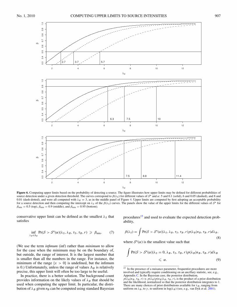
In particular, U(α, βmin) is the largest value of λS such thatPr(nS � S�(α)|λS, λB, τS) > 1 − βmin. This is illustrated forthree different values of βmin (panels) and three different valuesof α (line types) in Figure 6. Note that the upper limit increasesas βmin increases and as α decreases.
3.1.1. Illustrative Examples
To illustrate the difference between confidence bounds andupper limits, in the context of a detection process, we considertwo simple examples. The first is an extreme case where thebackground intensity is known to be identically zero, and evenone count in the source region would be classified as a detection.In this case, the upper limit is the smallest source intensity thatcan produce one count at a specified probability, e.g., a sourcewith intensity of 5 generates one or more counts at a probabilityof ≈99.7% (see Section 3.1). In contrast, if one count is seenin the source region, the upper bound of an equal-tail 99.7%interval on the source intensity is 8.9 (Gehrels 1986). Thus,while similar in magnitude, it can be seen that upper boundsand upper limits are different quantities, describing differentconcepts.
Second, consider a more realistic case where the backgroundis measured in a large region thought to be free of sources andscaled to the area covered by the source. Suppose that 800 countsare observed in an area 400 times larger than the source areaand 3 counts are seen in the putative source region itself. Thecredible interval for the source intensity may be calculated atvarious significance levels (Section 2.2; see also van Dyk et al.2001), and for this case we find that 68% credible interval withthe lower bound at 0 is [0, 2.1], and the 99.7% interval is [0, 8.3].But the question then arises as to whether the counts seen in thesource region are consistent with a fluctuation of the observedbackground or not. Since at a minimum 7 counts are neededfor a detection at a probability of 0.997 (corresponding to aGaussian-equivalent “3σ” detection), it is considered that thesource is not detected. The question then becomes how brightthe source would have to be in order to be detected with a certainprobability. Since a source of intensity 5.7 would have a 50%probability of producing sufficient counts for a detection, thissets an upper limit U(α = 0.003, βmin = 0.5) = 5.7 counts onthe undetected source’s intensity (for a Type I error α = 0.003and a Type II error β = 0.5; see Section 3.1). Note that thislimit is the same regardless of how many counts are actuallyseen within the source region, as expected from a quantity thatcalibrates the detection process. In contrast, the inference on thesource intensity is always dependent on the number of observedsource counts.
3.2. Unknown Background Intensity
So far our definition of an upper limit assumes that there areno unknown nuisance parameters, and in particular that λB isknown. Unfortunately, the probabilities in Equations (4) and(6) cannot be computed if λB is unknown. In this section, wedescribe several strategies that can be used in the more realisticsituation when λB is not known precisely.
The most conservative procedure ensures that the detectionprobability of the upper limit is greater than βmin for any possiblevalue of λB . Generally speaking, the larger λB is, the larger λS
must be in order to be detected with a given probability, and thusthe larger the upper limit. Thus, a useful upper limit requiresa finite range, ΛB , to be specified for λB . Given this range, a
No. 1, 2010 COMPUTING UPPER LIMITS TO SOURCE INTENSITIES 907
21018642
0.3
0.4
0.5
0.6
0.7
0.8
0.9
1.0
λS
β
2.7 3.7 5.7
21018642
0.3
0.4
0.5
0.6
0.7
0.8
0.9
1.0
λS
β
6.3 7.5 10
21018642
0.3
0.4
0.5
0.6
0.7
0.8
0.9
1.0
λS
β
7.5 8.8 11.4
Figure 6. Computing upper limits based on the probability of detecting a source. The figure illustrates how upper limits may be defined for different probabilities ofsource detection under a given detection threshold. The curves correspond to β(λS ) for different values of S� and α: 5 and 0.1 (solid), 6 and 0.05 (dashed), and 8 and0.01 (dash-dotted), and were all computed with λB = 3, as in the middle panel of Figure 4. Upper limits are computed by first adopting an acceptable probabilityfor a source detection and then computing the intercept on λS of the β(λS ) curves. The panels show the value of the upper limits for the different values of S� forβmin = 0.5 (top), βmin = 0.9 (middle), and βmin = 0.95 (bottom).
conservative upper limit can be defined as the smallest λS thatsatisfies
infλB∈ΛB
Pr(S > S�(α)|λS, λB, τS, τB, r) � βmin. (7)
(We use the term infimum (inf) rather than minimum to allowfor the case when the minimum may be on the boundary of,but outside, the range of interest. It is the largest number thatis smaller than all the numbers in the range. For instance, theminimum of the range {x > 0} is undefined, but the infimumis 0.) Unfortunately, unless the range of values ΛB is relativelyprecise, this upper limit will often be too large to be useful.
In practice, there is a better solution. The background countprovides information on the likely values of λB that should beused when computing the upper limit. In particular, the distri-bution of λB given nB can be computed using standard Bayesian
procedures15 and used to evaluate the expected detection prob-ability,
β(λS) =∫
Pr(S > S�(α)|λS, λB, τS, τB, r)p(λB |nB, τB, r)dλB,
(8)where S�(α) is the smallest value such that∫
Pr(S > S�(α)|λS = 0, λB, τS, τB, r)p(λB |nB, τB, r)dλB
� α. (9)
15 In the presence of a nuisance parameter, frequentist procedures are moreinvolved and typically require conditioning on an ancillary statistic, see, e.g.,Appendix C. In the Bayesian case, the posterior distribution,p(λB |nB, τB, r) ∝ p(λB )p(nB |λB, τB, r), is the product of a prior distributionand the likelihood, normalized so that the posterior distribution integrates to 1.There are many choices of prior distributions available for λB , ranging fromuniform on λB , to γ , to uniform in log(λB ) (see, e.g., van Dyk et al. 2001).
908 KASHYAP ET AL. Vol. 719
0 2 4 6 80.
00.
10.
20.
30.
4
λB
Pos
terio
r D
istr
ibut
ion
0 5 10 15
0.0
0.2
0.4
0.6
0.8
1.0
λS
β
α = 0.1, s*=6α = 0.05, s*=7α = 0.01, s*=9
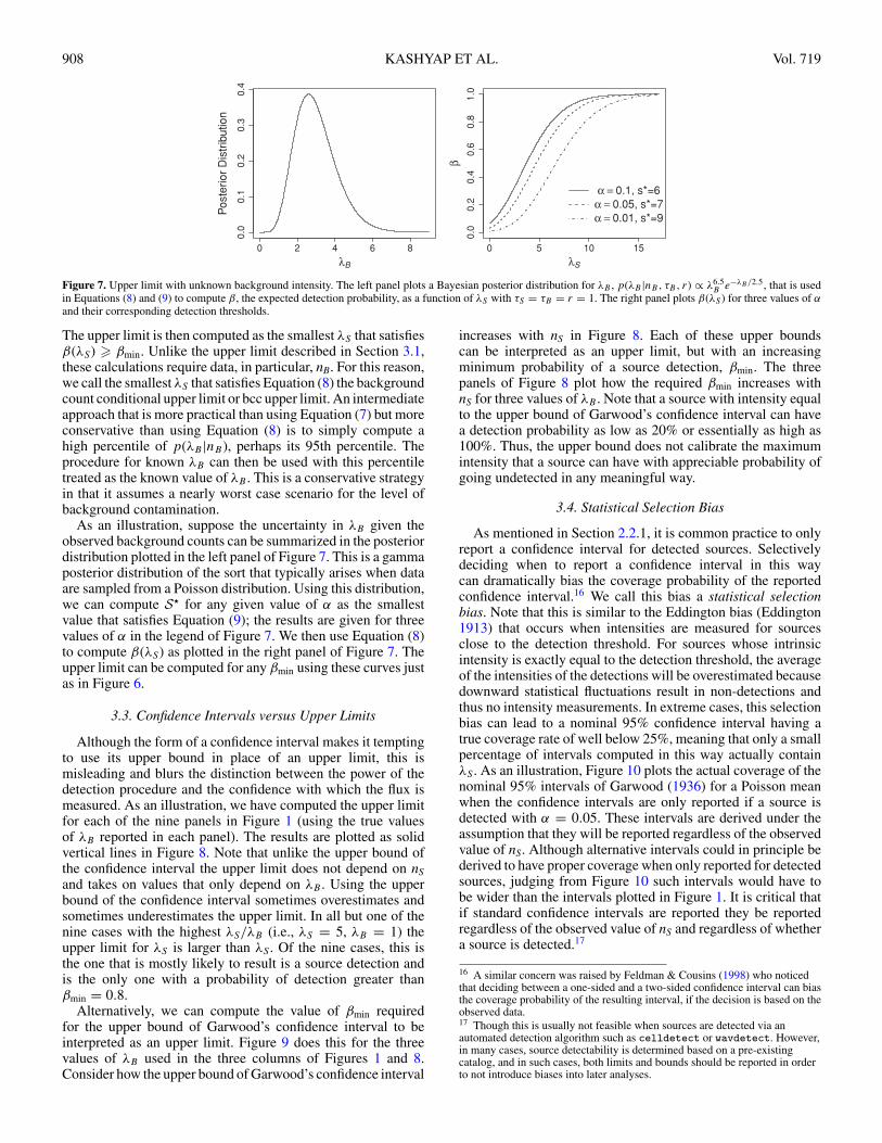
Figure 7. Upper limit with unknown background intensity. The left panel plots a Bayesian posterior distribution for λB , p(λB |nB, τB, r) ∝ λ6.5B e−λB/2.5, that is used
in Equations (8) and (9) to compute β, the expected detection probability, as a function of λS with τS = τB = r = 1. The right panel plots β(λS ) for three values of α
and their corresponding detection thresholds.
The upper limit is then computed as the smallest λS that satisfiesβ(λS) � βmin. Unlike the upper limit described in Section 3.1,these calculations require data, in particular, nB. For this reason,we call the smallest λS that satisfies Equation (8) the backgroundcount conditional upper limit or bcc upper limit. An intermediateapproach that is more practical than using Equation (7) but moreconservative than using Equation (8) is to simply compute ahigh percentile of p(λB |nB), perhaps its 95th percentile. Theprocedure for known λB can then be used with this percentiletreated as the known value of λB . This is a conservative strategyin that it assumes a nearly worst case scenario for the level ofbackground contamination.
As an illustration, suppose the uncertainty in λB given theobserved background counts can be summarized in the posteriordistribution plotted in the left panel of Figure 7. This is a gammaposterior distribution of the sort that typically arises when dataare sampled from a Poisson distribution. Using this distribution,we can compute S� for any given value of α as the smallestvalue that satisfies Equation (9); the results are given for threevalues of α in the legend of Figure 7. We then use Equation (8)to compute β(λS) as plotted in the right panel of Figure 7. Theupper limit can be computed for any βmin using these curves justas in Figure 6.
3.3. Confidence Intervals versus Upper Limits
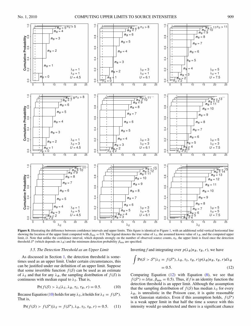
Although the form of a confidence interval makes it temptingto use its upper bound in place of an upper limit, this ismisleading and blurs the distinction between the power of thedetection procedure and the confidence with which the flux ismeasured. As an illustration, we have computed the upper limitfor each of the nine panels in Figure 1 (using the true valuesof λB reported in each panel). The results are plotted as solidvertical lines in Figure 8. Note that unlike the upper bound ofthe confidence interval the upper limit does not depend on nSand takes on values that only depend on λB . Using the upperbound of the confidence interval sometimes overestimates andsometimes underestimates the upper limit. In all but one of thenine cases with the highest λS/λB (i.e., λS = 5, λB = 1) theupper limit for λS is larger than λS . Of the nine cases, this isthe one that is mostly likely to result is a source detection andis the only one with a probability of detection greater thanβmin = 0.8.
Alternatively, we can compute the value of βmin requiredfor the upper bound of Garwood’s confidence interval to beinterpreted as an upper limit. Figure 9 does this for the threevalues of λB used in the three columns of Figures 1 and 8.Consider how the upper bound of Garwood’s confidence interval
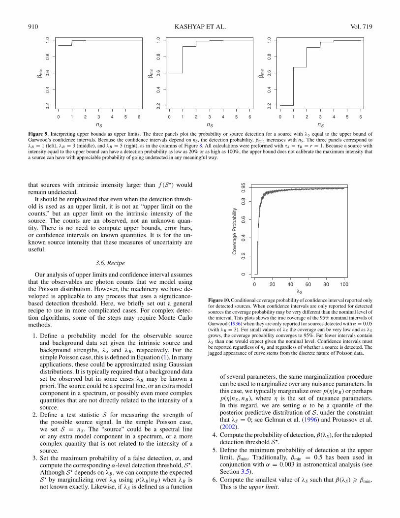
increases with nS in Figure 8. Each of these upper boundscan be interpreted as an upper limit, but with an increasingminimum probability of a source detection, βmin. The threepanels of Figure 8 plot how the required βmin increases withnS for three values of λB . Note that a source with intensity equalto the upper bound of Garwood’s confidence interval can havea detection probability as low as 20% or essentially as high as100%. Thus, the upper bound does not calibrate the maximumintensity that a source can have with appreciable probability ofgoing undetected in any meaningful way.
3.4. Statistical Selection Bias
As mentioned in Section 2.2.1, it is common practice to onlyreport a confidence interval for detected sources. Selectivelydeciding when to report a confidence interval in this waycan dramatically bias the coverage probability of the reportedconfidence interval.16 We call this bias a statistical selectionbias. Note that this is similar to the Eddington bias (Eddington1913) that occurs when intensities are measured for sourcesclose to the detection threshold. For sources whose intrinsicintensity is exactly equal to the detection threshold, the averageof the intensities of the detections will be overestimated becausedownward statistical fluctuations result in non-detections andthus no intensity measurements. In extreme cases, this selectionbias can lead to a nominal 95% confidence interval having atrue coverage rate of well below 25%, meaning that only a smallpercentage of intervals computed in this way actually containλS . As an illustration, Figure 10 plots the actual coverage of thenominal 95% intervals of Garwood (1936) for a Poisson meanwhen the confidence intervals are only reported if a source isdetected with α = 0.05. These intervals are derived under theassumption that they will be reported regardless of the observedvalue of nS. Although alternative intervals could in principle bederived to have proper coverage when only reported for detectedsources, judging from Figure 10 such intervals would have tobe wider than the intervals plotted in Figure 1. It is critical thatif standard confidence intervals are reported they be reportedregardless of the observed value of nS and regardless of whethera source is detected.17
16 A similar concern was raised by Feldman & Cousins (1998) who noticedthat deciding between a one-sided and a two-sided confidence interval can biasthe coverage probability of the resulting interval, if the decision is based on theobserved data.17 Though this is usually not feasible when sources are detected via anautomated detection algorithm such as celldetect or wavdetect. However,in many cases, source detectability is determined based on a pre-existingcatalog, and in such cases, both limits and bounds should be reported in orderto not introduce biases into later analyses.
No. 1, 2010 COMPUTING UPPER LIMITS TO SOURCE INTENSITIES 909
0 5 10 15 20 25
0.0
0.2
0.4
0.6
0.8
1.0
Cu
mu
lati
ve P
rob
abili
ty
nS = 0
nS = 1
nS = 2
nS = 3
nS = 4nS = 5nS > 5
U = 4.5λS = 1λB = 1
0 5 10 15 20 25
0.0
0.2
0.4
0.6
0.8
1.0
nS = 0nS = 1
nS = 2
nS = 3
nS = 4
nS = 5
nS = 6nS = 7
nS = 8 nS > 8
U = 6.1λS = 1λB = 3
0 5 10 15 20 25
0.0
0.2
0.4
0.6
0.8
1.0
nS < 2nS = 2
nS = 3
nS = 4
nS = 5
nS = 6
nS = 7
nS = 8nS = 9
nS = 10nS = 11nS > 11
U = 7.5λS = 1λB = 5
0 5 10 15 20 25
0.0
0.2
0.4
0.6
0.8
1.0
Cu
mu
lati
ve P
rob
abili
ty
nS = 0nS = 1
nS = 2
nS = 3
nS = 4
nS = 5
nS = 6nS = 7
nS = 8nS > 8
U = 4.5λS = 3λB = 1
0 5 10 15 20 25
0.0
0.2
0.4
0.6
0.8
1.0
nS < 2nS = 2
nS = 3
nS = 4
nS = 5
nS = 6
nS = 7
nS = 8nS = 9
nS = 10nS = 11...
U = 6.1λS = 3λB = 3
0 5 10 15 20 25
0.0
0.2
0.4
0.6
0.8
1.0
nS < 3nS = 3
nS = 4nS = 5
nS = 6
nS = 7
nS = 8
nS = 9
nS = 10nS = 11
nS = 12nS = 13
...
U = 7.5λS = 3λB = 5
0 5 10 15 20 25
0.0
0.2
0.4
0.6
0.8
1.0
λS
Cu
mu
lati
ve P
rob
abili
ty
nS < 2nS = 2
nS = 3
nS = 4
nS = 5
nS = 6
nS = 7
nS = 8nS = 9
nS = 10nS = 11...
U = 4.5λS = 5λB = 1
0 5 10 15 20 25
0.0
0.2
0.4
0.6
0.8
1.0
λS
...nS = 3nS = 4
nS = 5
nS = 6
nS = 7
nS = 8
nS = 9
nS = 10nS = 11
nS = 12nS = 13
...
U = 6.1λS = 5λB = 3
0 5 10 15 20 25
0.0
0.2
0.4
0.6
0.8
1.0
λS
...nS = 4nS = 5
nS = 6nS = 7
nS = 8
nS = 9
nS = 10
nS = 11
nS = 12nS = 13
nS = 14nS = 15
...
U = 7.5λS = 5λB = 5
Figure 8. Illustrating the difference between confidence intervals and upper limits. This figure is identical to Figure 1, with an additional solid vertical horizontal lineshowing the location of the upper limit computed with βmin = 0.8. The legend denotes the true value of λS , the assumed known value of λB , and the computed upperlimit, U . Note that unlike the confidence interval, which depends strongly on the number of observed source counts, nS, the upper limit is fixed once the detectionthreshold S� (which depends on λB ) and the minimum detection probability βmin are specified.
3.5. The Detection Threshold as an Upper Limit
As discussed in Section 1, the detection threshold is some-times used as an upper limit. Under certain circumstances, thiscan be justified under our definition of an upper limit. Supposethat some invertible function f (S) can be used as an estimateof λS and that for any λB , the sampling distribution of f (S) iscontinuous with median equal to λS . That is,
Pr(f (S) > λS |λS, λB, τS, τB, r) = 0.5. (10)
Because Equation (10) holds for any λS , it holds for λS = f (S�).That is,
Pr(f (S) > f (S�)|λS = f (S�), λB, τS, τB, r) = 0.5. (11)
Inverting f and integrating over p(λB |nB, τB, r), we have∫Pr(S > S�|λS = f (S�), λB, τS, τB, r)p(λB |nB, τB, r)dλB
= 0.5. (12)
Comparing Equation (12) with Equation (8), we see thatf (S�) = U(α, βmin = 0.5). Thus, if f is an identity function thedetection threshold is an upper limit. Although the assumptionthat the sampling distribution of f (S) has median λS for everyλB , is unrealistic in the Poisson case, it is quite reasonablewith Gaussian statistics. Even if this assumption holds, f (S�)is a weak upper limit in that half the time a source with thisintensity would go undetected and there is a significant chance
910 KASHYAP ET AL. Vol. 719
0 1 2 3 4 5 6
0.2
0.4
0.6
0.8
1.0
nS
β min
0 1 2 3 4 5 6
0.2
0.4
0.6
0.8
1.0
nS
β min
0 1 2 3 4 5 6
0.2
0.4
0.6
0.8
1.0
nS
β min
Figure 9. Interpreting upper bounds as upper limits. The three panels plot the probability or source detection for a source with λS equal to the upper bound ofGarwood’s confidence intervals. Because the confidence intervals depend on nS, the detection probability, βmin increases with nS. The three panels correspond toλB = 1 (left), λB = 3 (middle), and λB = 5 (right), as in the columns of Figure 8. All calculations were preformed with τS = τB = r = 1. Because a source withintensity equal to the upper bound can have a detection probability as low as 20% or as high as 100%, the upper bound does not calibrate the maximum intensity thata source can have with appreciable probability of going undetected in any meaningful way.
that sources with intrinsic intensity larger than f (S�) wouldremain undetected.
It should be emphasized that even when the detection thresh-old is used as an upper limit, it is not an “upper limit on thecounts,” but an upper limit on the intrinsic intensity of thesource. The counts are an observed, not an unknown quan-tity. There is no need to compute upper bounds, error bars,or confidence intervals on known quantities. It is for the un-known source intensity that these measures of uncertainty areuseful.
3.6. Recipe
Our analysis of upper limits and confidence interval assumesthat the observables are photon counts that we model usingthe Poisson distribution. However, the machinery we have de-veloped is applicable to any process that uses a significance-based detection threshold. Here, we briefly set out a generalrecipe to use in more complicated cases. For complex detec-tion algorithms, some of the steps may require Monte Carlomethods.
1. Define a probability model for the observable sourceand background data set given the intrinsic source andbackground strengths, λS and λB , respectively. For thesimple Poisson case, this is defined in Equation (1). In manyapplications, these could be approximated using Gaussiandistributions. It is typically required that a background dataset be observed but in some cases λB may be known apriori. The source could be a spectral line, or an extra modelcomponent in a spectrum, or possibly even more complexquantities that are not directly related to the intensity of asource.
2. Define a test statistic S for measuring the strength ofthe possible source signal. In the simple Poisson case,we set S = nS . The “source” could be a spectral lineor any extra model component in a spectrum, or a morecomplex quantity that is not related to the intensity of asource.
3. Set the maximum probability of a false detection, α, andcompute the corresponding α-level detection threshold, S�.Although S� depends on λB , we can compute the expectedS� by marginalizing over λB using p(λB |nB) when λB isnot known exactly. Likewise, if λS is defined as a function
λS
Cov
erag
e P
roba
bilit
y
0 20 40 60 80 100
00.
20.
40.
60.
80.
95
Figure 10. Conditional coverage probability of confidence interval reported onlyfor detected sources. When confidence intervals are only reported for detectedsources the coverage probability may be very different than the nominal level ofthe interval. This plots shows the true coverage of the 95% nominal intervals ofGarwood (1936) when they are only reported for sources detected with α = 0.05(with λB = 3). For small values of λS the coverage can be very low and as λS
grows, the coverage probability converges to 95%. Far fewer intervals containλS than one would expect given the nominal level. Confidence intervals mustbe reported regardless of nS and regardless of whether a source is detected. Thejagged appearance of curve stems from the discrete nature of Poisson data.
of several parameters, the same marginalization procedurecan be used to marginalize over any nuisance parameters. Inthis case, we typically marginalize over p(η|nB) or perhapsp(η|nS, nB ), where η is the set of nuisance parameters.In this regard, we are setting α to be a quantile of theposterior predictive distribution of S, under the constraintthat λS = 0; see Gelman et al. (1996) and Protassov et al.(2002).
4. Compute the probability of detection, β(λS), for the adopteddetection threshold S�.
5. Define the minimum probability of detection at the upperlimit, βmin. Traditionally, βmin = 0.5 has been used inconjunction with α = 0.003 in astronomical analysis (seeSection 3.5).
6. Compute the smallest value of λS such that β(λS) � βmin.This is the upper limit.
No. 1, 2010 COMPUTING UPPER LIMITS TO SOURCE INTENSITIES 911
4. EXAMPLE: SIGNAL-TO-NOISE RATIO
We focus below on signal-to-noise (S/N)-based detectionat a single location as an example application. The S/N wasthe primary statistic used for detecting sources in high-energyastrophysics before the introduction of maximum-likelihoodand wavelet-based methods. Typically, S/N = 3 was used as thedetection threshold, corresponding to α = 0.003 in the Gaussianregime. Here, we apply the recipe in Section 3.6 to derive anupper limit with S/N-based detection. Our methods can alsobe applied to more sophisticated detection algorithms such assliding-cell detection methods such as celldetect (Harndenet al. 1984; Dobrzycki et al. 2000; Calderwood et al. 2001), andwavelet-based detection methods such as pwdetect (Damianiet al. 1997), zhdetect (Vikhlinin et al. 1997), wavdetect(Freeman et al. 2002), etc. Implementation of our techniquefor these methods will vary in detail, and we leave thesedevelopments for future work.
We begin with a Gaussian probability model for the sourceand background counts (Step 1 in Section 3.6)
nB |(λB, r, τB ) ∼ N (μ = rτBλB, σ =√
rτBλB)
nS |(λS, λB, τS) ∼ N (μ = τS(λS + λB), σ =√
τS(λS + λB)) ,
(13)
where λB and λS are non-negative. We assume that the source isentirely contained within the source cell and that the PSF doesnot overlap the background cell. We can estimate λB and λS bysetting nB and nS to their expectations (method of moments), as
λ̂B = nB
rτB
and λ̂S = nS
τS
− nB
rτB
. (14)
The variance of λ̂S is
var(λ̂S) = λS
τS
+(τS + rτB)λB
rτSτB
(15)
which we can estimate by plugging in λ̂S and λ̂B as
v̂ar(λ̂S) = nS
τ 2S
+nB
r2τ 2B
. (16)
To use the S/N as a detection criterion, we define (Step 2 inSection 3.6)
S = λ̂S√v̂ar(λ̂S)
= rτBnS − τSnB√r2τ 2
BnS + τ 2S nB
. (17)
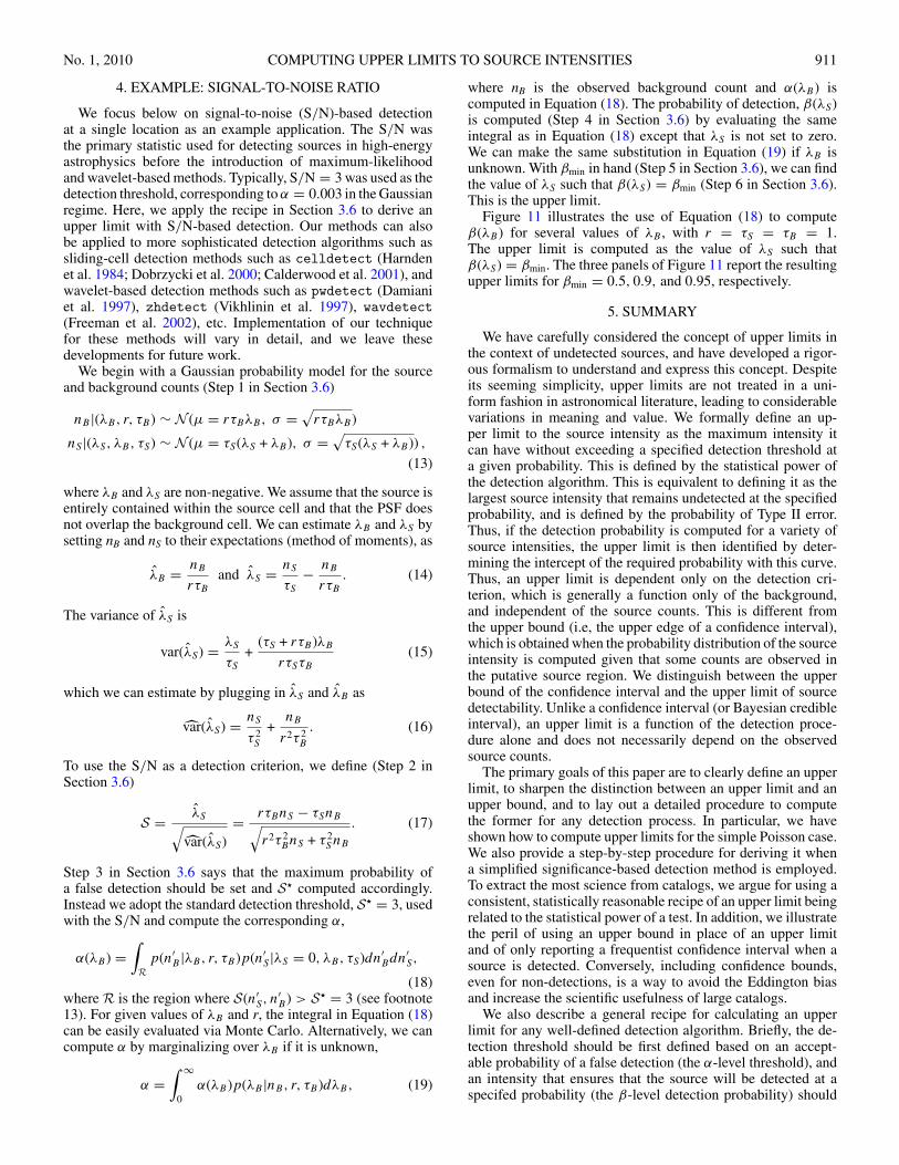
Step 3 in Section 3.6 says that the maximum probability ofa false detection should be set and S� computed accordingly.Instead we adopt the standard detection threshold, S� = 3, usedwith the S/N and compute the corresponding α,
α(λB) =∫R
p(n′B |λB, r, τB )p(n′
S |λS = 0, λB, τS)dn′Bdn′
S,
(18)where R is the region where S(n′
S, n′B ) > S� = 3 (see footnote
13). For given values of λB and r, the integral in Equation (18)can be easily evaluated via Monte Carlo. Alternatively, we cancompute α by marginalizing over λB if it is unknown,
α =∫ ∞
0α(λB)p(λB |nB, r, τB )dλB, (19)
where nB is the observed background count and α(λB) iscomputed in Equation (18). The probability of detection, β(λS)is computed (Step 4 in Section 3.6) by evaluating the sameintegral as in Equation (18) except that λS is not set to zero.We can make the same substitution in Equation (19) if λB isunknown. With βmin in hand (Step 5 in Section 3.6), we can findthe value of λS such that β(λS) = βmin (Step 6 in Section 3.6).This is the upper limit.
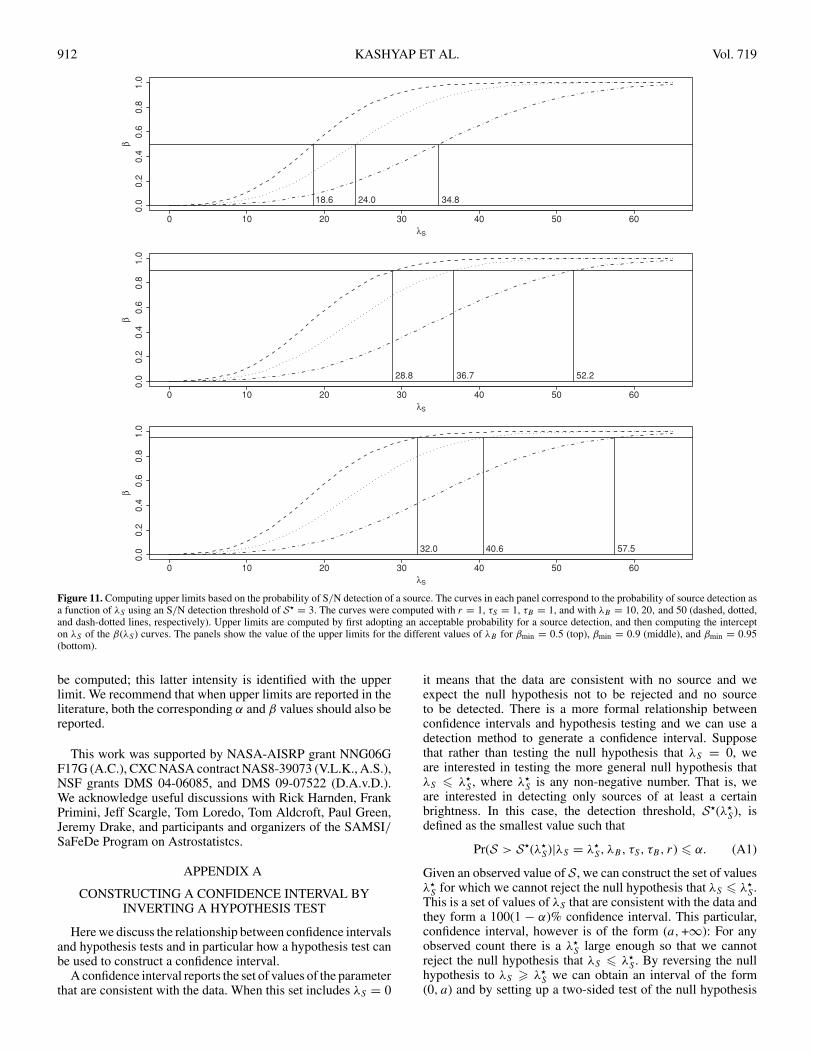
Figure 11 illustrates the use of Equation (18) to computeβ(λB) for several values of λB , with r = τS = τB = 1.The upper limit is computed as the value of λS such thatβ(λS) = βmin. The three panels of Figure 11 report the resultingupper limits for βmin = 0.5, 0.9, and 0.95, respectively.
5. SUMMARY
We have carefully considered the concept of upper limits inthe context of undetected sources, and have developed a rigor-ous formalism to understand and express this concept. Despiteits seeming simplicity, upper limits are not treated in a uni-form fashion in astronomical literature, leading to considerablevariations in meaning and value. We formally define an up-per limit to the source intensity as the maximum intensity itcan have without exceeding a specified detection threshold ata given probability. This is defined by the statistical power ofthe detection algorithm. This is equivalent to defining it as thelargest source intensity that remains undetected at the specifiedprobability, and is defined by the probability of Type II error.Thus, if the detection probability is computed for a variety ofsource intensities, the upper limit is then identified by deter-mining the intercept of the required probability with this curve.Thus, an upper limit is dependent only on the detection cri-terion, which is generally a function only of the background,and independent of the source counts. This is different fromthe upper bound (i.e, the upper edge of a confidence interval),which is obtained when the probability distribution of the sourceintensity is computed given that some counts are observed inthe putative source region. We distinguish between the upperbound of the confidence interval and the upper limit of sourcedetectability. Unlike a confidence interval (or Bayesian credibleinterval), an upper limit is a function of the detection proce-dure alone and does not necessarily depend on the observedsource counts.
The primary goals of this paper are to clearly define an upperlimit, to sharpen the distinction between an upper limit and anupper bound, and to lay out a detailed procedure to computethe former for any detection process. In particular, we haveshown how to compute upper limits for the simple Poisson case.We also provide a step-by-step procedure for deriving it whena simplified significance-based detection method is employed.To extract the most science from catalogs, we argue for using aconsistent, statistically reasonable recipe of an upper limit beingrelated to the statistical power of a test. In addition, we illustratethe peril of using an upper bound in place of an upper limitand of only reporting a frequentist confidence interval when asource is detected. Conversely, including confidence bounds,even for non-detections, is a way to avoid the Eddington biasand increase the scientific usefulness of large catalogs.
We also describe a general recipe for calculating an upperlimit for any well-defined detection algorithm. Briefly, the de-tection threshold should be first defined based on an accept-able probability of a false detection (the α-level threshold), andan intensity that ensures that the source will be detected at aspecifed probability (the β-level detection probability) should
912 KASHYAP ET AL. Vol. 719
0 10 20 30 40 50 60
0.0
0.2
0.4
0.6
0.8
1.0
λS
β
18.6 24.0 34.8
0 10 20 30 40 50 60
0.0
0.2
0.4
0.6
0.8
1.0
λS
β
2.257.638.82
0 10 20 30 40 50 60
0.0
0.2
0.4
0.6
0.8
1.0
λS
β
32.0 40.6 57.5
Figure 11. Computing upper limits based on the probability of S/N detection of a source. The curves in each panel correspond to the probability of source detection asa function of λS using an S/N detection threshold of S� = 3. The curves were computed with r = 1, τS = 1, τB = 1, and with λB = 10, 20, and 50 (dashed, dotted,and dash-dotted lines, respectively). Upper limits are computed by first adopting an acceptable probability for a source detection, and then computing the intercepton λS of the β(λS ) curves. The panels show the value of the upper limits for the different values of λB for βmin = 0.5 (top), βmin = 0.9 (middle), and βmin = 0.95(bottom).
be computed; this latter intensity is identified with the upperlimit. We recommend that when upper limits are reported in theliterature, both the corresponding α and β values should also bereported.
This work was supported by NASA-AISRP grant NNG06GF17G (A.C.), CXC NASA contract NAS8-39073 (V.L.K., A.S.),NSF grants DMS 04-06085, and DMS 09-07522 (D.A.v.D.).We acknowledge useful discussions with Rick Harnden, FrankPrimini, Jeff Scargle, Tom Loredo, Tom Aldcroft, Paul Green,Jeremy Drake, and participants and organizers of the SAMSI/SaFeDe Program on Astrostatistcs.
APPENDIX A
CONSTRUCTING A CONFIDENCE INTERVAL BYINVERTING A HYPOTHESIS TEST
Here we discuss the relationship between confidence intervalsand hypothesis tests and in particular how a hypothesis test canbe used to construct a confidence interval.
A confidence interval reports the set of values of the parameterthat are consistent with the data. When this set includes λS = 0
it means that the data are consistent with no source and weexpect the null hypothesis not to be rejected and no sourceto be detected. There is a more formal relationship betweenconfidence intervals and hypothesis testing and we can use adetection method to generate a confidence interval. Supposethat rather than testing the null hypothesis that λS = 0, weare interested in testing the more general null hypothesis thatλS � λ�
S , where λ�S is any non-negative number. That is, we
are interested in detecting only sources of at least a certainbrightness. In this case, the detection threshold, S�(λ�
S), isdefined as the smallest value such that
Pr(S > S�(λ�S)|λS = λ�
S, λB, τS, τB, r) � α. (A1)
Given an observed value of S, we can construct the set of valuesλ�
S for which we cannot reject the null hypothesis that λS � λ�S .
This is a set of values of λS that are consistent with the data andthey form a 100(1 − α)% confidence interval. This particular,confidence interval, however is of the form (a, +∞): For anyobserved count there is a λ�
S large enough so that we cannotreject the null hypothesis that λS � λ�
S . By reversing the nullhypothesis to λS � λ�
S we can obtain an interval of the form(0, a) and by setting up a two-sided test of the null hypothesis
No. 1, 2010 COMPUTING UPPER LIMITS TO SOURCE INTENSITIES 913
that λS = λ�S against the alternative hypothesis that λS �= λ�
S wecan obtain an interval of the more common form (a, b).
APPENDIX B
THE RELATIONSHIP BETWEEN UPPER LIMITS ANDTHE POWER OF THE TEST
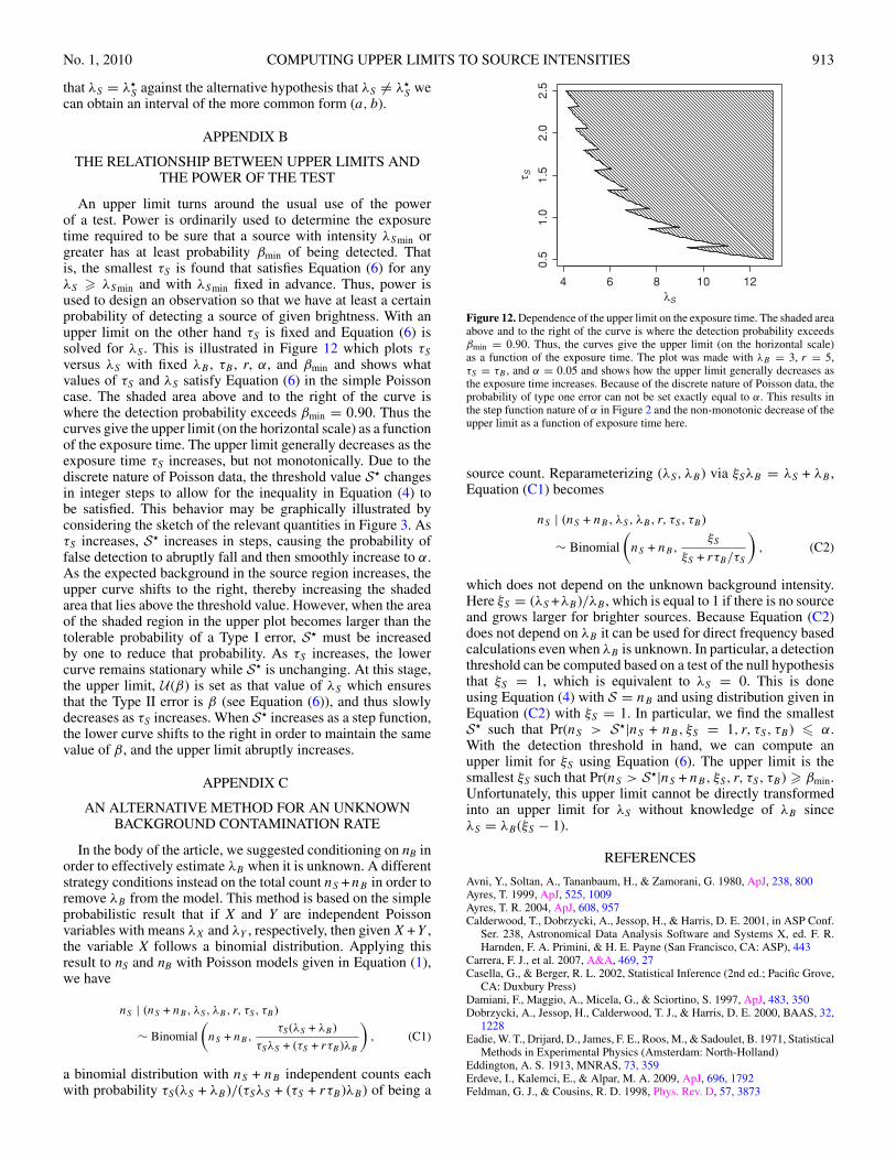
An upper limit turns around the usual use of the powerof a test. Power is ordinarily used to determine the exposuretime required to be sure that a source with intensity λSmin orgreater has at least probability βmin of being detected. Thatis, the smallest τS is found that satisfies Equation (6) for anyλS � λSmin and with λSmin fixed in advance. Thus, power isused to design an observation so that we have at least a certainprobability of detecting a source of given brightness. With anupper limit on the other hand τS is fixed and Equation (6) issolved for λS . This is illustrated in Figure 12 which plots τS
versus λS with fixed λB , τB , r, α, and βmin and shows whatvalues of τS and λS satisfy Equation (6) in the simple Poissoncase. The shaded area above and to the right of the curve iswhere the detection probability exceeds βmin = 0.90. Thus thecurves give the upper limit (on the horizontal scale) as a functionof the exposure time. The upper limit generally decreases as theexposure time τS increases, but not monotonically. Due to thediscrete nature of Poisson data, the threshold value S� changesin integer steps to allow for the inequality in Equation (4) tobe satisfied. This behavior may be graphically illustrated byconsidering the sketch of the relevant quantities in Figure 3. AsτS increases, S� increases in steps, causing the probability offalse detection to abruptly fall and then smoothly increase to α.As the expected background in the source region increases, theupper curve shifts to the right, thereby increasing the shadedarea that lies above the threshold value. However, when the areaof the shaded region in the upper plot becomes larger than thetolerable probability of a Type I error, S� must be increasedby one to reduce that probability. As τS increases, the lowercurve remains stationary while S� is unchanging. At this stage,the upper limit, U(β) is set as that value of λS which ensuresthat the Type II error is β (see Equation (6)), and thus slowlydecreases as τS increases. When S� increases as a step function,the lower curve shifts to the right in order to maintain the samevalue of β, and the upper limit abruptly increases.
APPENDIX C
AN ALTERNATIVE METHOD FOR AN UNKNOWNBACKGROUND CONTAMINATION RATE
In the body of the article, we suggested conditioning on nB inorder to effectively estimate λB when it is unknown. A differentstrategy conditions instead on the total count nS + nB in order toremove λB from the model. This method is based on the simpleprobabilistic result that if X and Y are independent Poissonvariables with means λX and λY , respectively, then given X +Y ,the variable X follows a binomial distribution. Applying thisresult to nS and nB with Poisson models given in Equation (1),we have
nS | (nS + nB, λS, λB, r, τS, τB )
∼ Binomial
(nS + nB,
τS (λS + λB )
τSλS + (τS + rτB )λB
), (C1)
a binomial distribution with nS + nB independent counts eachwith probability τS(λS + λB)/(τSλS + (τS + rτB)λB) of being a
4 6 8 10 12
0.5
1.0
1.5
2.0
2.5
λS
τ S
Figure 12. Dependence of the upper limit on the exposure time. The shaded areaabove and to the right of the curve is where the detection probability exceedsβmin = 0.90. Thus, the curves give the upper limit (on the horizontal scale)as a function of the exposure time. The plot was made with λB = 3, r = 5,τS = τB , and α = 0.05 and shows how the upper limit generally decreases asthe exposure time increases. Because of the discrete nature of Poisson data, theprobability of type one error can not be set exactly equal to α. This results inthe step function nature of α in Figure 2 and the non-monotonic decrease of theupper limit as a function of exposure time here.
source count. Reparameterizing (λS, λB) via ξSλB = λS + λB ,Equation (C1) becomes
nS | (nS + nB, λS, λB, r, τS, τB )
∼ Binomial
(nS + nB,
ξS
ξS + rτB/τS
), (C2)
which does not depend on the unknown background intensity.Here ξS = (λS +λB)/λB , which is equal to 1 if there is no sourceand grows larger for brighter sources. Because Equation (C2)does not depend on λB it can be used for direct frequency basedcalculations even when λB is unknown. In particular, a detectionthreshold can be computed based on a test of the null hypothesisthat ξS = 1, which is equivalent to λS = 0. This is doneusing Equation (4) with S = nB and using distribution given inEquation (C2) with ξS = 1. In particular, we find the smallestS� such that Pr(nS > S�|nS + nB, ξS = 1, r, τS, τB ) � α.With the detection threshold in hand, we can compute anupper limit for ξS using Equation (6). The upper limit is thesmallest ξS such that Pr(nS > S�|nS + nB, ξS, r, τS, τB ) � βmin.Unfortunately, this upper limit cannot be directly transformedinto an upper limit for λS without knowledge of λB sinceλS = λB(ξS − 1).
REFERENCES
Avni, Y., Soltan, A., Tananbaum, H., & Zamorani, G. 1980, ApJ, 238, 800Ayres, T. 1999, ApJ, 525, 1009Ayres, T. R. 2004, ApJ, 608, 957Calderwood, T., Dobrzycki, A., Jessop, H., & Harris, D. E. 2001, in ASP Conf.
Ser. 238, Astronomical Data Analysis Software and Systems X, ed. F. R.Harnden, F. A. Primini, & H. E. Payne (San Francisco, CA: ASP), 443
Carrera, F. J., et al. 2007, A&A, 469, 27Casella, G., & Berger, R. L. 2002, Statistical Inference (2nd ed.; Pacific Grove,
CA: Duxbury Press)Damiani, F., Maggio, A., Micela, G., & Sciortino, S. 1997, ApJ, 483, 350Dobrzycki, A., Jessop, H., Calderwood, T. J., & Harris, D. E. 2000, BAAS, 32,
1228Eadie, W. T., Drijard, D., James, F. E., Roos, M., & Sadoulet, B. 1971, Statistical
Methods in Experimental Physics (Amsterdam: North-Holland)Eddington, A. S. 1913, MNRAS, 73, 359Erdeve, I., Kalemci, E., & Alpar, M. A. 2009, ApJ, 696, 1792Feldman, G. J., & Cousins, R. D. 1998, Phys. Rev. D, 57, 3873
914 KASHYAP ET AL. Vol. 719
Freeman, P. E., Kashyap, V., Rosner, R., & Lamb, D. Q. 2002, ApJS, 138,185
Garwood, F. 1936, Biometrika, 28, 437Gehrels, N. 1986, ApJ, 303, 335Gelman, A., Meng, X.-L., & Stern, H. 1996, Statistica Sinica, 6, 733Gilman, D. A., Hurley, K. C., Seward, F. D., Schnopper, H. W., Sullivan, J. D.,
& Metzger, A. E. 1986, ApJ, 300, 453Gradshteyn, I. S., & Ryzhik, I. M. 1980, Table of Integrals, Series, and Products
(4th ed.; San diego, CA: Academic Press)Harnden, F. R., Jr., Fabricant, D., Harris, D., & Schwartz, D. 1984, SAO Spc.
Rep. 393Hughes, J. P., Chugai, N., Chevalier, R., Lundquist, P., & Schlegel, E. 2007, ApJ,
670, 1260Isobe, T., Feigelson, E. D., & Nelson, P. I. 1986, ApJ, 306, 490Kashyap, V., et al. 2008, HEAD, 10.0302Kraft, R. P., Burrows, D. N., & Nousek, J. A. 1991, ApJ, 374, 344Loewenstein, M., Kusenko, A., & Biermann, P. L. 2009, ApJ, 700, 426Mandelkern, M. 2002, Stat.Sci., 17, 149
Loredo, T. 1992, in Statistical Challenges in Modern Astronomy, ed. E. D.Feigelson & G. J. Babu (New York: Springer-Verlag), 275
Marshall, H. 1992, in Statistical Challenges in Modern Astronomy I, ed. E. D.Feigelson & G. J. Babu (Berlin: Springer), 247
Mattox, J. R., et al. 1996, ApJ, 461, 396Park, T., van Dyk, D. A., & Siemiginowska, A. 2008, ApJ, 688, 807Pease, D. O., Kashyap, V. L., & Drake, J. J. 2006, ApJ, 636, 436Perez-Torres, M. A., Zandanel, F., Guerrero, M. A., Pal, S., Profumo, S., Prada,
F., & Panessa, F. 2009, MNRAS, 396, 2237Protassov, R., van Dyk, D. A., Connors, A., Kashyap, V., & Siemiginowska, A.
2002, ApJ, 571, 545Rudnick, L., & Lemmerman, J. A. 2009, ApJ, 697, 1341Schlegel, E. M., & Petre, R. 1993, ApJ, 412, L29van Dyk, D. A., Connors, A., Kashyap, V. L., & Siemiginowska, A. 2001, ApJ,
548, 224Vikhlinin, A., Forman, W., & Jones, C. 1997, ApJ, 474, L7Weisskopf, M. C., Wu, K., Trimble, V., O’Dell, S. L., Elsner, R. F., Zavlin, V. E.,
& Kouvelioutou, C. 2007, ApJ, 657, 1026