on computing thom polynomials - department of mathematics
TRANSCRIPT

CE
UeT
DC
olle
ctio
n
On computing Thom polynomials
Balazs Komuves
Supervisor: Laszlo Feher
Submitted to
Central European University, Budapest
Department of Mathematics and its Applications
In partial fulfillment of the requirements
for the degree of Doctor of Philosophy
Budapest, Hungary
2010

CE
UeT
DC
olle
ctio
n

CE
UeT
DC
olle
ctio
n
Abstract
The subject matter of this thesis is the computation of Thompolynomials of singularities of maps, in particular Thom-Boardmansingularity classes. A “singularity” means a type of local behaviourof maps between smooth (or analytic) manifolds; the simplest ex-ample is the differential being degenerate. It is well known that thecohomology class of the (closure of the) locus in the source manifoldwhere a map has a given singularity can be expressed as a polyno-mial of the characteristic classes of the map. This multivariate poly-nomial, which only depends on the singularity and the dimensions,is called the Thom polynomial of the singularity. Even though theabove phenomenon was observed by Thom more than 50 years ago,there are still only a few examples where we can explicitly calculatethese polynomials. In this work, we contribute both new methodsof computations, and explicit calculations of some previously un-known Thom polynomials. In particular, we discover a connectionbetween localization formulae for contact singularities and basichypergeometric series; we present a new geometric construction tocompactify some moduli spaces related to Thom-Boardman classes;and we give new formulae for the Thom polynomials of some secondorder Thom-Boardman singularities.

CE
UeT
DC
olle
ctio
n
Table of Contents
Introduction vi
Notations and conventions viii
1. Partitions viii
2. Symmetric functions and characteristic classes viii
3. A list of various notations ix
Chapter 1. First order - The Thom-Porteous formula 10
1.1. Existence of the Thom polynomial and stability 10
1.2. Porteous’ embedded resolution 12
1.3. Equivariant localization 13
1.4. Restriction equations 14
1.5. Grobner degeneration 16
Chapter 2. Primer on singularity theory 17
2.1. Singularities 17
2.2. Thom-Boardman classes 18
2.3. Thom polynomials 20
2.3.1. Known Thom polynomials 21
Chapter 3. Localization of Thom polynomials 22
3.1. Localization for contact singularities 22
3.2. The substitution trick 26
3.3. Principal specialization 28
3.3.1. An algorithmic approach 30
3.4. Some analytic computations 31
3.4.1. Σ1, A1 32
3.4.2. Σ2, III2,2 32
3.4.3. A2, Σ11 36
Chapter 4. Second order - Σij 40
4.1. Equivalence of the different definitions 40
4.2. Ronga’s formula 41
4.3. Localization 43
4.3.1. The probe model for Thom-Boardman singularities 43
4.3.2. The compactifications 46
4.3.3. The localization formula 56
4.4. Explicit formulae for the coefficients 57
4.5. Combinatorics 61
4.5.1. The coefficients for Σi,1 61
4.5.2. The coefficients for Σ22 64
iv

CE
UeT
DC
olle
ctio
n
v
Chapter 5. Third order - A3 68
5.1. The probe model for Σijk 68
5.2. Morin singularities 70
5.2.1. The A3 singularity 74
Appendix 80
A.1. Multivariate differentials 80
A.2. Formulae for symmetric polynomials 82
A.3. Localization of equivariant cohomology classes 85
A.4. Pushforward formulae 88
A.5. Basic hypergeometric series 93
Bibliography 95

CE
UeT
DC
olle
ctio
n
Introduction
This thesis reports on the state of the author’s ongoing investigation on the subject ofcomputing Thom polynomials of singularities of maps, in particular Thom-Boardman singu-larity classes.
A “singularity” here means a type of local behaviour of maps between smooth (analytic)spaces; a very simple example is the vanishing of the differential of the map. There is ageneral local-global principle, which says the global topological properties of (closed) spacescan be read off from local geometric data. Two well-known examples of this phenomenon are:the Gauss-Bonnet theorem, which expresses the Euler characteristic of a manifold from thecurvature; and the Poincare-Hopf theorem, which expresses the Euler characteristic from thesingularities of a vector field on the manifold. Thom polynomials, proposed by Rene Thomaround 1950, are also a manifestation of this principle; in a sense, they are a generalizationof the latter example. The basic observation is that given a singularity (that is, a type oflocal behaviour), the (co)homological properties of the locus where a map has the given typeof behaviour depends only on the homotopy type of the map, and not on the fine details ofthe map itself. This can be made quantitative: the cohomology class of the locus can beexpressed as a polynomial of the characteristic classes of the map; this polynomial is calledthe Thom polynomial of the singularity.
Our focus in this work is the problem of computing these polynomials. However, onequickly bumps into the philosophical question of what ‘computing’ means: First, these poly-nomials can be expressed in many different forms (eg. polynomials in Chern roots; polyno-mials in Chern classes; linear combination of Schur functions; variations of the latter twofor the difference alphabet; pushforward formulae; iterated residue formulae; localizationformulae; etc.) which are often very hard to convert to each other; second, it is easy to writedown formulae which are very hard to evaluate in concrete cases (eg. even small cases areintractable by today’s home computers).
Our answer (which is by no means final) is that we prefer expressing the Thom polyno-mials as linear combinations of Schur polynomials in the difference alphabet; the motivationfor this form is that it is elegant, unique, relatively compact, the coefficients are nonnega-tive integers, they do not depend on the dimensions of the source and target spaces, andthere is some evidence that they have very rich combinatorics. Furthermore, we seek (whenpossible) computationally effective methods to compute these coefficients; of course, we stillprefer (closed) formulae.
In the last 10 years, there was a new wave of activity in the field; thanks to works of G.Berczi, A. Buch, L. Feher, M. Kazarian, A. Nemethi, P. Pragacz, R. Rimanyi, A. Szenes,the author, and others, we now know much more about both concrete examples and thestructures behind Thom polynomials. However explicit computations are still hard, evenusing computers; and that is the subject matter this thesis contributes to, with both newformulae and new methods.
vi

CE
UeT
DC
olle
ctio
n
vii
Organization of the material. The first two chapters are introductory: The firstchapter introduces informally the notion of Thom polynomials and the basic methods tocompute them, using the Thom-Porteous formula as a running example. The next chapterrecalls some basic definitions of singularity theory. The third chapter deals with the generallocalization formula for contact singularities; it introduces a new idea to evaluate them,which can be also used to derive closed formulae. The fourth chapter investigates the specificcase of second order Thom-Boardman singularities from multiple viewpoints. In the final,fifth chapter, we show how to modify a geometric idea introduced in the previous chapterto compute the Thom polynomials of the A3 singularity. The appendices collect togethervarious results we use during the text.
New results and statement of originality. The sections 3.2, 3.3, 3.4 in Chapter3; sections 4.4, 4.3, 4.5 in Chapter 4, and Section 5.2.1 contain new results. From theabove, Theorem 4.2.2, Section 4.4 (except the proof of Theorem 4.4.3), and Section 4.5.1was published in the article [FK06] joint with Laszlo Feher. The rest of the above is myoriginal work. Furthermore, I gave new proofs of some known statements; in particular, theproofs of Lemma 3.1.2, Theorem A.3.7 and Theorem A.4.4 are my own work; Theorem 4.2.1of Ronga [Ron72] is also reproved as a side-effect of this work.
Acknowledgments. The author would like to thank Gergely Berczi, Laszlo Feher,Frances Kirwan, Andras Nemethi, Richard Rimanyi and Andras Szenes for various helpand discussions; and his family and friends for support. During this work, he was supportedfinancially by the Central European University (2003-2006), the Alfred Renyi Institute ofMathematics (2007-2009), and by a Marie Curie fellowship during his six-month stay at theUniversity of Oxford (2006-2007).
This work wouldn’t exist without computers. In particular we used the following softwareand resources: The MapleTM computer algebra system; John Stembridge’s SF package forMaple [Ste05] (to compute with symmetric polynomials); Matthias Franz’s Convex pack-age for Maple [Fra09] (to compute with convex polyhedra); the Glasgow Haskell Compiler[GHC] for the Haskell programming language [PJ03]; Sloane’s On-Line Encyclopedia ofInteger Sequences [OEIS]; and last, but not least, various digital libraries. The thesis wastypeset with LATEX. The figures were produced with several different software, which shouldremain nameless, as the range varied from the “rather inconvenient” to the “exceptionallypainful”.

CE
UeT
DC
olle
ctio
n
Notations and conventions
Unless specifically stated, we will always work over the field of complex numbers; ie. vec-tor spaces are complex vector spaces, vector bundles are complex vector bundles, algebraicvarieties are complex algebraic varieties—in particular, Pn is the complex projective space—,etc. Cohomology is singular cohomology, the default coefficient ring is the field Q of ratio-nal numbers (just to be on the safe side; however, most results should work, without anymodification, with integer coefficients).
1. Partitions. Partitions are by definition finite nonincreasing sequences of positiveintegers. They will be usually denoted by the greek letters λ, χ, µ and ν. Our conven-tion is that we allow arbitrary number of zeros at the end of partitions, that is, we treat(µ1, µ2, . . . , µk) and (µ1, µ2, . . . , µk, 0, 0, . . . , 0) as the same object; this is often useful in for-mulae. The length of a partition µ, which is the number of positive elements, is denotedby `(µ) = k; the weight, or sum, is denoted by |µ| =
∑µi. Repeated numbers are often
denoted by exponents, ie. (23, 14) = (2, 2, 2, 1, 1, 1, 1). The dual partition1 of µ, denoted byµ, is defined by
µi = maxj : µj ≥ i
.
This is an involution on the set of partitions; note that `(µ) = µ1. We denote by λ± µ thepointwise addition (resp. subtraction) of the sequences; the latter isn’t necessarily a partition.
A partition µ is a subpartition of an other partition λ, denoted by µ ⊂ λ, if µi ≤ λifor all i. If µ ⊂ (nk), then its complement µ is defined by (µ)i = n − µk+1−i; we omitthe ‘block’ (nk) from the notation, as it will be always clear from the context. The reversesequence (µk, µk−1, . . . , µ1) is denoted by revµ.
The ‘stairway’ partition (n, n− 1, n− 2, . . . , 1) is used often enough to deserve a specialnotation, for which we will use bne.
2. Symmetric functions and characteristic classes. Let c1, c2, c3 . . . and s1, s2, s3, . . .denote two sequences of formal variables related by the equation
(1 + c1t+ c2t2 + c3t
3 + · · · ) · (1− s1t+ s2t2 − s3t3 +− · · · ) = 1.
The convention is that c0 = s0 = 1, and c<0 = s<0 = 0. If we have a polinomial ringk[x1, . . . , xn], we can specialize these formal variables to the elementary and complete sym-metric functions, respectively; the subring generated by either of the two sequences is exactlythe ring of symmetric polynomials k[x1, . . . , xn]Sn . The same thing works with the limitn→∞, the ring
Λ = ←−limn
k[x1, x2, . . . , xn]Sn
being called the ring of symmetric functions.If we have a complex vector bundle E → M (or more generally, a formal difference of
two vector bundles), we can specialize to the Chern and Segre2 classes ci(E) and si(E) inH2i(M), respectively (and that’s why we use the notations ci and si instead of the ei and hiwhich are the standard in the theory of symmetric functions).
1the term conjugate partition is also used2the literature has a sign ambiguity in the definition of Segre classes; for example our convention agrees
with that of [FP98] but differs by (−1)i from that of [Ful98]
viii

CE
UeT
DC
olle
ctio
n
ix
The Schur polynomials are symmetric polynomials parameterized by partitions; they arearguably the most important symmetric functions, and they give an additive basis in thering of symmetric functions. Given a partition µ = (µ1, µ2, . . . , µk), we define the Schurpolynomial sµ by the formula
sµ = det[sµi+j−i]k×k = det[ceµi+j−i]µ1×µ1 ;
in particular3, s(i) = si and s(1i) = ci. As before, we can define the Schur class sλ(E) ∈H2|λ|(M) of a (complex) vector bundle E by substituting its Chern (or Segre) classes intothe formula above.
3. A list of various notations. Finally we try to make the life of the reader easier byassembling a (necessarily partial) list of the various notations used in this thesis.
H∗(Y ) singular cohomology with coefficients in QH∗G(Y ) G-equivariant cohomology
AGi (X) G-equivariant Chow groups (see [EG98a])f∗ pullback along the map f (of cohomology classes, or vector bundles)π∗ pushforward (or Gysin map); if π : X → Y then π∗ : H∗(X)→ H∗+codimπ(Y )
[X ⊂ Y ] the (equivariant) cohomology class represented by X in H∗(Y ) (or H∗G(Y ));
often denoted simply by [X]e(V ), [V ] (equivariant) Euler class of a vector bundle or representation; [V ]—as a short-
hand for [0 ⊂ V ],—is used only when there is no danger of confusionNZX normal bundle (or bundle of normal cones, if X is singular) of Z in X
Sn the symmetric group of order nV ∨ dual representation
SymkV symmetric tensor powers of V∧kV antisymmetric tensor powers of VSλV Schur functors; S(k)V = SymkV and S(1,1,...,1)V = ∧kVcurry the natural isomorphism curry : Hom(U ⊗ V,W )→ Hom(U,Hom(V,W ))4
U V if V ≤ U , this is the image of U ⊗V under the quotient map U ⊗U → Sym2U ;isomorphic to ((U/V )⊗ V )⊕ (Sym2V ). Similarly for U ≤ V .
i j the dimension analogue of the previous entry: dim(U i V j) = i j. If j ≤ i,we have i j = j(i− j) + j(j + 1)/2
Jd(V,W ) the space of d-jets from (V, 0) to (W, 0); that is,Jd(V,W ) = ⊕dk=1Hom(SymkV,W )
J d (V,W ) jets with injective linear partJ (V,W ) shorthand for Jd(V,W ) where d (possibly infinity) is clear from the context,
or not importantJd(n,m) shorthand for Jd(Cn,Cm)Jd(V ) shorthand for Jd(V,C), which is a (nilpotent) ringEd(V ) C⊕ Jd(V ); space of jets of functions, a local ring with unit
Diffd(V ) jets of diffeomorphisms; shorthand for J d (V, V )
3the equation s(i) = si motivates our choice of conventions. S(k) = Symk is another lucky corollary.4‘currying’ is a standard terminology for this in computer science and logic, named after the logician
Haskell Brooks Curry.

CE
UeT
DC
olle
ctio
n
Chapter 1. First order - The Thom-Porteous formula
The aim of this part of the thesis is to introduce the methods, phenomena and notationson the simplest and most widely studied case, which we denote by Σi. Correspondingly, weclaim no originality for the results presented in this chapter. See also [FR06] for a shortoverview of different methods.
The sentence
“the map f : Nn →Mm has Σi singularity at the point x ∈ N”
means simply that the rank of the differential dxf drops by i, that is (assuming m ≥ n),dim ker(dxf) = i. The cohomological properties of the locus
Σi(f) =x ∈ N : dim ker(dxf) ≥ i
(1)
are widely studied in different contexts, including topology, algebraic geometry, etc. Theclass1 [Σi(f)] in the cohomology ring (also in the Chow ring, etc.) is given by the Thom-Porteous formula [Por71]:[
Σi(f)]
= s(im−n+i)(f∗TM − TN) = det[cm−n+i+j−k(f∗TM − TN)]k,j∈i×i ∈ H∗(N ; Z)
assuming some mild transversality conditions (or in the complex analytic case, that the locushas the expected codimension i(m− n+ i)). Chapter 9 of [FP98] lists some applications ofthis formula in algebraic geometry.
1.1. Existence of the Thom polynomial and stability
Thom was interested in the set (1), and more generally, its analogue for other singularities.He proposed the following theorem:
Theorem 1.1.1 ([Tho56, HK57]). Let Nn and Mm be two smooth (real) manifolds, andΣ be a singularity, that is, a Diff(n)×Diff(m) invariant subvariety of Jd(n,m). Σ defines asubset (which we also denote by Σ) of the global jet space Jd(N,M). There exists a polynomialP in two set of variables c1, c2, . . . and d1, d2, . . . such that for a map f : N → M , whosejet is transversal to the singularity subset Σ, the cohomology class [Σ(f)] ∈ H∗(N ; Z2) of thelocus
Σ(f) =x ∈ N : the jet of f at x belongs to Σ
is given by substituting the Stiefel-Whitney classes of TN and f∗TM into the polynomial P :
[Σ(f)] = P (w1(TN), w2(TN), . . . ; f∗w1(TM), f∗w2(TM), . . . )
This polynomial is called the Thom polynomial of the singularity.
Remark. The theorem remains true if we replace R with C, ‘smooth’ by ‘analytic’, Z2 withZ and Stiefel-Whitney classes with Chern classes. In the following, we will focus on thecomplex case.
1With some abuse of notation, we will always write [X] instead of [X], as only closed subvarieties represent
classes anyway.
10

CE
UeT
DC
olle
ctio
n
11
Let us demonstrate this theorem for the Σi singularity defined above. The derivative dxfof f at x ∈ N is a linear map in Hom(TxN,Tf(x)M). Assembling these maps for all x ∈ N ,we get a section df of the vector bundle ξ = Hom(TN, f∗TM). The structure group of thisbundle is GLn ×GLm; since Σi (the set of corank i linear maps) is invariant for the action ofthis structure group, we can define the “smeared” version Σi(TN, f∗TM) by
Σi(TN, f∗TM) =
(ϕ, x) ∈ Hom(TN, f∗TM) : x ∈ N, ϕ ∈ Σi(TxN,Tf(x)M)
Clearly, we have
Σi(f) = (df)−1 Σi(TN, f∗TM),
and if the section df is transversal to the stratification given by the Σi(TN, f∗TM) sets, wealso have [
Σi(f) ⊂ N]
= (df)∗[Σi(TN, f∗TM) ⊂ Hom(TN, f∗TM)
].
Note that at this point, we could have any two vector bundles An, Bm and a (nice,transversal) section σ ∈ ΓHom(A,B) instead of TN and f∗TM and df . In particular, wecan apply the construction to the universal bundles
Un = pr∗1(Cn ×GLn EGLn
)Um = pr∗2
(Cm ×GLm EGLm
)on the classifying space BGLn ×BGLm; and get a universal class
[Σi] = [Σi ⊂ Hom(Un, Um)] ∈ H∗(Hom(Un, Um)) ∼= H∗(BGLn ×BGLm) = H∗GLn×GLm
(pt).
This construction is compatible with pull-backs, and for any bundles An and Bm over a(paracompact) manifold M there is a map Φ : M → BGLn × BGLm such that Φ∗Un = A
and Φ∗Um = B; putting these together, we get that Σi(A,B) = Φ∗Σi(Un, Um), and thus
[Σi(A,B)] = Φ∗[Σi(Un, Um)].
Finally, let us remark that H∗(BGLn × BGLm) is a (graded) polynomial ring, generated bythe Stiefel-Whitney (or Chern, in the complex case) classes of Un and Um, and the pullbackΦ∗ is given by substituting the Stiefel-Whitney (Chern) classes of A and B into these gener-ators. Thus the universal class [Σi] is the Thom polynomial P .
Next, let us show that this polynomial can be expressed as a polynomial in the (virtual)Stiefel-Whitney or Chern classes of the (formal) difference bundle B −A, which are defined(in the Chern case) by the equation∑
k≥0
ck(B −A) · tk =
∑mj=0 cj(B) · tj∑ni=0 ci(A) · ti
∈ H∗(M; Z)[[t]],
where t is a formal variable. Observe that if E is a third vector bundle, then for the sectionσ ⊗ id ∈ ΓHom(A⊕ E,B ⊕ E), defined simply by
(σ ⊗ id)x(a, e) = (σx(a), e),
we have Σi(σ) = Σi(σ⊗id) already as a set (the transversality conditions are also equivalent).Choosing E to be an orthogonal complement2 of A in some large trivial bundle CK , we get
2Orthogonal complements do not exist in the category of holomorphic vector bundles, but here we are
dealing simply with complex vector bundles.

CE
UeT
DC
olle
ctio
n
12
that[Σi(A,B)] = [Σi(A⊕A⊥, B ⊕A⊥)] = [Σi(CK , B ⊕A⊥)],
but c(CK) = 1 and c(B ⊕ A⊥) = c(B − A), from which it follows that P (c(A), c(B)) =P (1, c(B − A)). Since this works for any compact manifold M, it must be true for the uni-versal polynomial, too.
Rephrasing in the language of equivariant cohomology, we demonstrated that the Thompolynomial is a universal class (characteristic class), in particular, it is the GLn × GLm-equivariant cohomology class represented by the closed subvariety Σi ⊂ Hom(An, Bm), whereA and B are the standard GLn resp. GLm representations (optionally thought as equivariantvector bundles over the point). Also, this class cannot be arbitrary: It lies in the subringgenerated by ck(B −A).
1.2. Porteous’ embedded resolution
The “classical” method for calculating the cohomology class [Σ] ∈ H∗(X) represented bya singular subvariety Σ of a smooth ambient variety X is to find an embedded resolution ofthe pair (X,Σ), that is, smooth varieties Σ ⊂ Y and a map π : Y → X such that
• π−1(Σ) = Σ,• Σ is a resolution of Σ,• and the following diagram commutes:
Σj−−−−→ Y
πy yπΣ i−−−−→ X
In this situation we have
[Σ ⊂ X] = i∗[1] = i∗π∗[1] = π∗j∗[1] = π∗[Σ ⊂ Y ]
This is useful if it is easy to compute [Σ ⊂ Y ]; typically Y will be a vector bundleand Σ a subbundle, in which case [Σ ⊂ Y ] is the Euler class of the quotient bundle. Thesame construction works in the equivariant setting, where a Lie group G acts on X andY such that Σ and Σ are invariant and π is equivariant. Y is choosed such that the push-forward map π∗ : H∗
G(Y )→ H∗G(X) can be computed, for example using the formulae in A.4.
Porteous’ construction [Por71] uses a straightforward generalization of the usual blow-up construction in algebraic geometry. Using the notation above, the roles are played asfollows:
X : Hom(V n,Wm)
Σ : Σi =ϕ ∈ Hom(V,W ) : dim ker(ϕ) ≥ i
Y : Gri(V )× Hom(V,W )
Σ : Σi =
(R,ϕ) ∈ Gri(V )× Hom(V,W ) : R ⊂ ker(ϕ)
π : pr2 = projection to the second coordinate
and the whole diagram is GL(V ) × GL(W )-equivariant. In this situtation, Σ is a linearsubbundle of Y , and the quotient bundle is Hom(R, π∗W ), where R ⊂ π∗V is the tautological

CE
UeT
DC
olle
ctio
n
13
rank i vector bundle over Gri(V ); thus, using the pushforward formula (38), Theorem A.4.1,
[Σi(V,W )] = π∗ctop
(Hom(R, π∗W )
)= π∗s(im)(π
∗W −R) = (−1)imπ∗s(mi)(R− π∗W )
= (−1)im+i(n−i)s(mi−(n−i)i)(V −W )
= s(im−n+i)(W − V )
Remark. In this toy case, the weaker version of the pushforward formula (36) would be alsosufficient, though resulting in a more involved derivation.
1.3. Equivariant localization
This is a variation and generalization of the previous method, which, in the context ofcomputing Thom polynomials, first appeared in [BSz06]. The first idea is that we can useequivariant localization to compute the pushforward, see Corollary A.3.3: This works in thegeneral case, where we may not have such a nice formula as in the case of the Grassman-nian; of course, then it may be not easy to evaluate the resulting localization formula either.Second, we may not need a full resolution: Since localization works quite well with singularvarieties, a partial resolution is often enough.
The typical situation is that we want to compute the (torus-equivariant) class of aninvariant affine variety Z ⊂ V , and we can present the closure Z as an union of (infinitelymany) linear subspaces; that is, we have an (equivariant) vector bundle Y ⊂M× V over acompact varietyM, such that pr2(Y ) = Z. Then we can apply Theorem A.3.7, and localizeonM:
[Z ⊂ V ]T =∑p∈MT
[Yp ⊂ V ]TeT(TpM)
assuming (for simplicity) that M is smooth and has isolated fixed point set MT. Here Ypdenotes the fiber pr−1
1 (p) over p ∈M.
In the case of Z = Σi, the situation is the same as described in the previous section:
V = Hom(V,W )
M = Gri(V )
Y =
(R,ϕ) ∈ Gri(V )× Hom(V,W ) : R ⊂ ker(ϕ)
which results in the formula
[Σi(V,W )] =∑I∈(n
i)
eT(Hom(I,W )eT(Hom(I, n− I))
=
=∑I∈(n
i)
∏ml=1
∏j∈I(θl − αj)∏
k/∈I∏j∈I(αk − αj)
∈ Z[α1, . . . , αn, θ1, . . . , θm]Sn×Sm .

CE
UeT
DC
olle
ctio
n
14
1.4. Restriction equations
This method was introduced by Richard Rimanyi, [Rim01]; see also [FR04]. It is basedon the geometry of orbits: It works best when the symmetries are large, and there are onlyfinitely many orbits. This is probably the most efficient method for small cases; on the otherhand, its scope is limited. While we don’t use this method directly in this thesis, it was theoriginal motivation for Section 4.4.
Let V be a representation of a Lie group G, and X be an orbit; as usual, we want tocompute the G-equivariant class [X]G represented by the closure of X. The basic idea isvery simple: Take other G-orbits, and restrict the class [X] to them; if we can computethese restrictions, we get equations on [X], and if we have enough equations, maybe theydetermine [X] completely.
Lemma 1.4.1. Let Z be any G-orbit, and denote by jZ the embedding jZ : Z → V . Then
j∗Z [X]G =
0 Z ∩X = ∅eG(NZV ) Z = X
[NZX ⊂ NZV ]G Z ⊂ X
Note that the third case actually contains the other two. For a sketch of proof, see LemmaA.3.5 in the Appendix.
Remark. There is a different interpretation of this result. Let p ∈ Z be any point, andGp ⊂ G be its stabilizer subgroup. Then Z ∼= G/Gp,
j∗Z : H∗G(V ) = H∗
G(pt) → H∗G(Z) = H∗
Gp(pt)
and j∗Z is also the map induced by ip : Gp → G (we could also take any subgroup H < Gp, ormore generally, a Lie group morphism H → Gp, and restrict further). This viewpoint givesthe following interpretation of the lemma: For h : H → Gp
(ip h)∗[X]G =
0 Z ∩X = ∅eH((NZV )|p
)Z = X[
(NZX)|p ⊂ (NZV )|p]H
Z ⊂ X
While the original version is geometrically more natural, this version is effectively com-putable: We can take H to be a subgroup of Gp so that there exists a H-invariant comple-mentary subspace S to TpZ in TpV , then[
(NZX)|p ⊂ (NZV )|p]H
=[Np(S ∩X) ⊂ S
]H.
The basis of the theory is the following theorem:
Theorem 1.4.2 ([FR04]). Suppose there are finitely many G-orbits, and for any orbit Zthe Euler class of the normal bundle eG(NZV ) is not a zero divisor in H∗
G(Z). Then thefollowing set of equations for the class of a G-orbit X
j∗Z [X] =eG(NXV ) Z = X ‘principal equation’0 Z 6= X, codim(Z) ≤ codim(X) ‘homogeneous equations’
has a unique solution.

CE
UeT
DC
olle
ctio
n
15
Let’s apply this method to our running example: The group G = GLn×GLm acts on thespace of matrices Hom(Cn,Cm) = Matn×m from the left3 by
(L,R) ·A = LAR−1.
Let us suppose for simplicity that m ≥ n. The classification of the orbits is well-known:They are exactly the rank varieties Σk for 0 ≤ k ≤ n. For such an orbit Σk, we can choosea representative matrix of rank k
Ak =[Ik 00 0
]∈ Σk ⊂ Matn×m
with a k×k identity matrix on the top-left corner, and zero elsewhere. It is easy to computethe tangent space TAk
Σk of the orbit Σk at the Ak, by just applying (a basis of) the Liealgebra of infinitesimal actions g = gln × glm to Ak; it turns out that tangent space is
TAkΣk =
[∗ ∗∗ 0
], where ∗ is anything
< TAk
Matn×m ∼= Matn×m
As a side effect of this computation, we get the codimension formula
codim(Σk) = (n− k)(m− k).
A reasonably big subgroup (meaning that it is homotopy equivalent to it) Hk of the stabilizerof Ak is
Hk = ([
C 00 A
],
[C 00 B
]): C ∈ GLk, A ∈ GLn−k, B ∈ GLm−k
.
To do the computation however, it is better to restrict ourselves to the maximal tori. Letus denote by α1, . . . , αn and β1, . . . , βm the generators of H∗
Tn×Tm(pt); and by γ1, . . . , γk,αk+1, . . . , αn and βk+1, . . . , βm the corresponding generators of the the maximal torus Tk ofHk. Then the restriction map j∗k : H∗
G(pt)→ H∗Hk
(pt) is given by
αi 7→γi i ≤ kαi i > k
and βi 7→
γi i ≤ kβi i > k
A Hk-invariant normal space to Σk at Ak is
Sk = [
0 00 ∗
], where ∗ is anything
< TAk
Matn×m
with the Euler class
eTk(Sk) =
n∏i=k+1
m∏j=k+1
(βj − αi).
Gathering all this gives us a bunch of linear equations for the coefficients of the Thompolynomial (expressed as a polynomial in two set variables, one for GLn and one for GLm),which we can then solve using a computer algebra software, for example. In fact, in thisconcrete case the ‘principal equation’ imply all the others, since clearly the stabilizer of Σk
contains the stabilizers of Σi for all i < k. However, it is not easy in general to derive aformula which works for any k, n and m; this approach is algorithmic in nature. Of course,when we can guess the result, it is possible to prove it (in this case, for example by usingSylvester’s determinantal formula for the resultant); we omit this last step here.
3The usual convention to write linear maps as matrices is the transpose of what we use here; by that
convention, GLn would be the right group, etc.

CE
UeT
DC
olle
ctio
n
16
1.5. Grobner degeneration
For the sake of completeness, we have to mention the method of Grobner degeneration,which is well known among algebraic geometers. The basic fact here is that for an idealI C[V ] in a polynomial ring, there is a flat deformation to its initial ideal (see eg. [Eis95],Section 15.8). Many properties are invariant under flat deformation, in particular, the co-homology class, too (in the equivariant case, of course we need an invariant deformation).Since there are algorithms to compute the Grobner basis, and thus the initial ideal, thisgives us an algorithm to compute the (torus-equivariant) cohomology class represented by a(torus-invariant) affine variety given its ideal, since the geometry corresponding to the initialideal is just a bunch of coordinate subspaces with multiplicities.
For a very simple example, consider the plane C2 with the linear action of the multiplica-tive group U = C×〈ω〉 defined by
ω · (x, y) = (ω2x, ω3y),
with weights (2α, 3α). The subvariety Z defined by the equation y2 = x3 is invariant tothis action; let us compute it equivariant class [Z] ∈ H2
U (C2) = Z[α]. For this, consider thefollowing two U -invariant one-parameter deformations:
Zs = y2 = sx3 ⊂ C2 and
Z ′t = ty2 = x3 ⊂ C2, s, t ∈ C.
We have Z1 = Z ′1 = Z, and since both deformations are actually flat, [Z] = [Zs] = [Z ′t]; butZ0 is simply the line y = 0 with multiplicity 2, and Z ′0 is the other coordinate line x = 0,but with multiplicity 3. Thus both give the result [Z] = 6α. In general, instead of finding ex-plicit flat deformations, we can just compute the initial ideal using a Grobner basis algorithm.
However, in the situations studied in this thesis, more often that not we have no idea aboutthe ideals, and even if we knew them, the resulting Grobner basis computations would betoo big (even for computers). Nevertheless, this method can be useful for sub-computations;for example if we want to localize using Theorem A.3.7 over a base which is a singular toricvariety, we could in principle compute the virtual tangent Euler classes using Grobner bases.

CE
UeT
DC
olle
ctio
n
Chapter 2. Primer on singularity theory
Singularities, in our context, are types of local behaviour of (smooth or holomorphic)maps. We briefly collect the necessary definitions and facts here while referring to theliterature ([AVGL98] and the references therein) for the details, as our focus is on thecomputations.
2.1. Singularities
Probably the most natural definition is to consider germs of maps up to reparameteriza-tion of the source and the target: The “left-right” group
A = Diff(Cn, 0)× Diff(Cm, 0)
acts on the space of holomorphic germs (Cn, 0) → (Cm, 0). The equivalence classes (orbits)are called left-right singularity classes. An analogous definition can be given for smooth realgerms. A map f : M → N between manifolds has singularity type η at a point x ∈ M
if the germ of f at x in some (and thus, in any) local coordinate system belongs to theA-orbit of η. A singularity η is stable if for any map f having η singularity at x, and anysmall perturbation f ′, there exist an x′ close to x having the same singularity (in words: thesingularity cannot be eliminated by a small perturbation).
While A-equivalence is a certainly a natural notion, a better behaved classification is theso-called contact equivalence or K-equivalence, introduced by John Mather. Two germs fand f ′ are contact equivalent if there is a diffeomorphism germ h ∈ Diff(Cn) and a map germϕ ∈ J (Cn,GLm) such that
f ′(x) = ϕ(x)f(h(x)).
This can be also thought as a group action: the group K is
K = Diff(Cn)× J (Cn,GLm)
is acting (from the left) on J (n,m) by
((h, ϕ)f) (x) = ϕ(x)f(h−1(x)).
We will need some fundamental definitions.
Definition 2.1.1. The ideal of a singularity f = (f1, . . . , fm) ∈ J (n,m) is the ideal thegenerated by the component functions
If = (f1, . . . , fm) E(n)
where E(n) = C[[x1, . . . , xn]] is the ring of formal power series on Cn (similarly for truncatedpolynomial rings and other function rings). Clearly If is also an ideal in J (n) ⊂ E(n). Thelocal algebra of the singularity f is the quotient E(n)/If ; we will call the nilpotent quotient
Qf = J (n)/Ifthe quotient algebra. The dimension of the local algebra is called the algebraic multiplicity ofthe singularity; however, what actually is the important object for us is the quotient algebraand its dimension, which we will denote by µ:
µf = dim(Qf ) = dim(E(n)/If )− 1.
17

CE
UeT
DC
olle
ctio
n
18
Remark. The difference between E(n) and J (n) is that the former ring has a unit, whilethe latter is nilpotent: E(n) = C⊕J (n). Actually J (n) is the unique maximal ideal in E(n).There are versions of our main objects for both rings. The singularity theory literatureusually works with the ring of functions (or power series) and the local algebra, however forus it is more natural to work with the nilpotent objects. Note that the literature somtimesuse the symbols Q and µ for the local algebra and the algebraic multiplicity; but it wouldbe very inconvenient for us to follow this convention.
The most important results for us are the following:
Theorem 2.1.2 (Mather). K-equivalent stable germs are A-equivalent.
This shows that K-equivalence is a reasonably natural object.
Theorem 2.1.3 (Mather). Two map germs are K-equivalent if and only if their ideals aretaken into each other by a map induced by a germ of diffeomorphism in Diff(n).
Corollary 2.1.4. Two finitely determined map germs are K-equivalent if and only if theirlocal algebras (or equivalently, their quotient algebras) are isomorphic.
Remark. In this thesis, we are only dealing with finitely determined singularities: Theseare the singularities for which it is possible to determine for any jet whether it belongs to thegiven singularity by looking at only finitely many (depending on the singularity) derivatives.In this case, it is possible to truncate our rings at a given order; thus we can work with finitedimensional objects. In our viewpoint, this is not a real restriction.
2.2. Thom-Boardman classes
Since the complete classification of (say, contact) singularities is hopeless, it is clearlyuseful to have more coarse but better behaved classification schemes. The Thom-Boardmanclassification, introduced by Thom [Tho56] and clarified by Boardman [Boa67] (see also[Mat73]), is probably the most well-known and useful such scheme. It has the clear ad-vantage that the classes are indexed by discrete objects, namely, partitions (non-increasingfinite sequences of integers).
Definition 2.2.1 (Thom). For a (nice enough) map f : N →M , define the locus
Σi(f) =x ∈ N : dim(ker(dxf)) = i
.
Suppose that Σi(f) ⊂ N is smooth; then we can define Σij(f) to be Σj(f |Σif ), and similarly,for any index set I = i1, . . . , ik−1, let
ΣI,ik(f) = Σik(f |ΣIf ).
This definition is intuitive enough, but in the definition of Σi1i2...ik we have to assumethat the loci Σi1 , Σi1i2 , etc. are all smooth. Boardman gave a definition which cures thisproblem, but is much less intuitive.
Definition 2.2.2. Let U E(n) = f : Cn → C be an ideal of functions (or formal powerseries, etc.; and also similarly for the real case). The kth Jacobian extension ∆k(U) is theideal generated by U and all the k× k determinants det[∂ϕi/∂xj ], where xj is a (fixed) localcoordinate system and ϕi ∈ U . It will be convenient to also define ∆k(U) = ∆n−k+1(U).

CE
UeT
DC
olle
ctio
n
19
Figure 1. A Σ11 singularity; f : R2 → R2 is the vertical projection.
Definition 2.2.3. It is easy to see that
U = ∆0(U) ⊆ · · · ⊆ ∆k(U) ⊆ ∆k+1(U) ⊆ · · · ⊆ ∆n+1(U) = E(n).
The largest ∆k such that ∆k(U) ( E(n) is called the critical Jacobian extension.
Remark. The critical extension of an ideal U is ∆n−r = ∆r+1, where r = rankU is the rankof the ideal U , which is defined as rankU = dimC (m2 + U)/m2.
Definition 2.2.4 (Boardman). The germ f = (f1, . . . , fm), f(0) = 0 belongs to ΣI if theideal U = (f1, . . . , fm) E(n) has successive critical extensions
∆i1U, ∆i2∆i1U, ∆i3∆i2∆i1U, . . .
For a map g : N → M between manifolds, take a point x ∈ N and let (f1, . . . , fm) be thecoordinate functions of g in some local coordinate system around x and g(x); the definitionthen tells us the Boardman type of g at the point x.
Boardman proved that the singularity subsets defined this way are smooth submanifoldsof the appropriate jet spaces, and that they coincide with Thom’s definition when the latterapplies, by which we mean that ΣI
Thom(f) = (J f)−1(ΣIBoardman).
Porteous proposed a third definition in [Por83], based on his theory of intrinsic deriva-tives (see Section 4.3.1).
Remark. Thom-Boardman singularities of order d are d-determined, that is, it’s enough tolook at the first d differentials of a map to decide whether it belongs to the given Thom-Boardman class (this should be clear from Boardman’s definition). They are also stable inthe sense that if f : Cn → Cm belongs to ΣI , then so does f ⊕ idC : Cn+1 → Cm+1.

CE
UeT
DC
olle
ctio
n
20
2.3. Thom polynomials
Singularities describe local behaviour of maps, however, Thom polynomials are globalinvariants of singularities, describing (in cohomological terms) the “shape” of the singularlocus; they are an instance of the local-global principle.
Let us recall Theorem 1.1.1 from Chapter 1:
Theorem 2.3.1 ([Tho56, HK57]). Let Nn and Mm be two smooth, real (resp. complexanalytic) manifolds, and Σ be a singularity, that is, a Diffn × Diffm invariant subvariety ofJd(n,m). Σ defines a subset (which we also denote by Σ) of the global jet space Jd(N,M).There exists a universal polynomial P in two set of variables c1, . . . , cn and d1, . . . , dm, de-pending only on n, m and Σ, such that for a map f : N →M whose jet is transversal to thesingularity subset Σ, the cohomology class [Σ(f)] ∈ Hcodim(Σ)(N ; Z2) (resp. H2codim(Σ)(N ; Z))of the locus
Σ(f) =x ∈ N : the jet of f at x belongs to Σ
is given by substituting the Stiefel-Whitney (resp. Chern) classes of TN and f∗TM into thepolynomial P :
[Σ(f)] = P (w1(TN), w2(TN), . . . ; f∗w1(TM), f∗w2(TM), . . . )(2)
This polynomial is called the Thom polynomial of the singularity.
Sketch of proof. Consider the universal jet bundle JU → BU , and the Diffn×Diffm-equivariantcohomology class of the corresponding singularity set ΣU ⊂ JU . For any concrete casef : N →M , we can pull back from the universal case along the classifying map Φ : N → BU :
[Σ ⊂ J (N,M)] = [Φ−1(ΣU ) ⊂ J (N,M)] = Φ∗[ΣU ⊂ JU ];
furthermore, if f is transversal to Σ, then
[Σ(f) ⊂ N ] = [(Jf)−1(Σ) ⊂ N ] = (Jf)∗[Σ ⊂ J (N,M)] = (Jf)∗Φ∗[ΣU ⊂ JU ].
Since Diffn × Diffm is homotopy equivalent to GLn × GLm, the cohomology ring H∗(JU ) =H∗(BU ) in the universal situation will be a polynomial ring, and the pullback Φ∗ is givenby substituting the appropriate characteristic classes; consequently P = [ΣU ⊂ JU ]. Finally,(Jf)∗ is simply an isomorphism.
Remark. In the real case, the set of maps which are transversal to a given singularity aredense and open among all smooth maps; thus (2) is satisfied for almost any map f , and evenif f is “bad”, we can approximate it with “nice” maps to arbitrary precision. In the complexcase, this is no longer true. However, complex analytic maps are rigid, and we expect theformula to hold if the locus Σ(f) is a subvariety with the expected dimension (cf. [Ful98]).
In fact, the polynomial P cannot be arbitrary:
Theorem 2.3.2 ([Dam72]). For contact singularities, the polynomial P can be written as
P (c1, c2, . . . , cn; d1, d2, . . . , dm) = Q(h1, h2, h3, . . . )
where Q is again a polynomial, and hi is defined by the following identity of formal powerseries:
1 +∞∑k=1
hktk =
1 +∑m
j=1 djtj
1 +∑n
i=1 citi.

CE
UeT
DC
olle
ctio
n
21
The interpretation of hi in the above theorem is that they are the Chern classes of the ‘virtualdifference bundle’ f∗TM TN .
Remark. This theorem also holds for the Thom-Boardman classes.
Corollary 2.3.3. The polynomials P depend only on the relative codimension r = m− n,in the following sense:
Pn,m(c1, . . . , cn; d1, . . . , dn) = Pn+1,m+1(c1, . . . , cn, 0; d1, . . . , dn, 0).
Furthermore, the sequence k 7→ Pn+k,m+k eventually stabilizes.
We will call both P and Q the Thom polynomial of Σ (though we are more interestedin computing Q), and use the notation TpΣ(n,m) or just TpΣ for them. We will frequentlywrite Q as a linear combination of Schur polynomials (cf. Appendix A.2):
Qr(h1, h2, . . . ) =∑λ
eλr · sλ(h1, h2, . . . );
one observation motivating such a rendition is that the coefficients eλ are nonnegative integers(this was recently proven in [PW07a, PW07b], motivated by numerical evidence).
Another such observation is that the coefficients (when they appear) do not actuallydepend on the dimensions n and m at all; more precisely
eλr = e(µ,λ)r+1
where µ = µ(Σ) ∈ N is the dimension of the quotient algebra of the singularity. This meansthat if we “shift” the Thom polynomials by −r, they fit into an infinite series, called theThom series of the singularity; see [FR07], and Sections 3.1, 3.2 for the details.
2.3.1. Known Thom polynomials. To place our results into a context, we tried tocollect the list of previously known Thom polynomials here. We will (ab)use the notationΣ(r) for the Thom polynomial of Σ in relative codimension r.
• Σi(r) was calculated by Porteous [Por71] (but was already known to Giambelli).• Σij(r): A pushforward formula was given by Ronga [Ron72]. Some concrete cases,
eg. Σ2,1(0) and Σ2,2(−1) were computed. A simpler version (and a computer program)was given by Kazarian [Kaz06].• A2(r) was computed by Ronga as a special case of Σij .• A4(0) was computed by Gaffney [Gaf83].• A≤8(0), A≤4(1), Ia,b(0) for a + b ≤ 8 and some other examples were computed by
Rimanyi [Rim01], using the restriction equations method.• A3(r) was computed in [BFR02], [LP09].• I2,2(r): Kazarian gave a pushforward formula; the Thom series was computed in [FR07,
FR08], [Pra07].• A≤6(r): An iterated residue formula was given in [BSz06].• For I2,3(r), IIIa,b(r), a + b ≤ 6, A≤4(r), Σ21(r), and some other cases, localization
formulae were derived in [FR08], via “extrapolation” from previous results for smallr-s. They also computed the coefficients for an unnamed family which includes I2,2(r)and III2,3(r).• We computed Σi1(r) and Σij(−i+ 1) in [FK06].

CE
UeT
DC
olle
ctio
n
Chapter 3. Localization of Thom polynomials
In this chapter we study the general properties of localization formulae for singularities,which first appeared in [BSz06] in the context of Ad singularities, and were then generalizedin [FR08]. While the localization principle is very powerful in the sense that we can writedown formulae in cases which are not accessible to other methods, the resulting formulaeare notoriously hard to evaluate, since the terms are rational functions instead of polynomi-als. Summing rational functions in many variables with large denominators is pretty muchimpossible even using computers; while bringing the terms to a common denominator, thenumber of temporary terms suffer an exponential explosion, quickly exhausting the memoryof the computer. This happens for relatively small examples already: For example supposethat the denominators are products of binoms; today’s personal computers cannot handlethe case when the number of different factors (binoms) is about 30 or more.
However, Thom polynomials of singularities have some special properties (as opposed togeneral systems of polynomials in two sets of variables); in particular, we know a priori thatthey depend only on the (Chern classes of the) formal difference bundle c(f∗TM TN); andwe can exploit this fact to remedy the situation described above. It turns out that followingthis program leads quite naturally into the world of basic hypergeometric series; localizationformulae for singularities become q-hypergeometric identities.
Remark. Here we will work within the theory of contact singularities; while Thom-Boardmanclasses are not, in general, contact classes, everything holds for them too (see [Mat73]), asit is also easy to check in each concrete situation we will deal with in the thesis.
3.1. Localization for contact singularities
We present the basic ideas of [FR08], which give us insight into the structure of the(Thom polynomials) of contact singularities.
Recall the following notations:
F = (f1, f2, . . . , fm) ∈ J (n,m) the jet of the singularity
IF = (f1, f2, . . . , fm) J (n) the ideal of the singularity
QF = J (n)/IF the quotient algebra
µF = dimC(QF ) the algebraic multiplicity, shifted by −1
kQ = corank(IF ) minimal number of algebra generators of Q
rank(IF ) = dimC(m2 + IF )/m2 rank of the ideal
The basic construction is the following: For a (contact) singularity class Z ⊂ Jd(n,m)we want to find a vector bundle E → M which is an embedded partial resolution of (theclosure of) Z; we can then use equivariant localization on a compactification M to compute[Z] (the localization basically computes a pushforward). We will see that there exists a verynatural partial resolution satisfying our needs; that construction actually dates back to theseventies (Damon, Mather).
22

CE
UeT
DC
olle
ctio
n
23
Consider the map p : Z → Hilbµ(Jd(n)) ⊂ Grµ(Jd(n)), where Hilbµ(Jd(n)) is the (re-duced) Hilbert scheme of ideals of codimension µ in Jd(n), defined by mapping a jet F intoits ideal IF .
Proposition 3.1.1 ([FR08], Lemma 4.3). For any ideal I Jd(n), the closure of p−1(I) is
p−1(I) = I ⊗ Cm ⊂ Jd(n,m) = Jd(n)⊗ Cm.
Proof. Clearly p−1(I) ⊂ I⊗Cm. On the other hand it is open in I⊗Cm: Suppose f1, . . . , fmgenerates I, and b1, . . . , bm ∈ I are arbitrary elements of the ideal; we want to show that
f1 + εb1, . . . , fm + εbm
also generates I if ε ∈ C is small enough. For this, write bi =∑rijfj for some rij ∈ R =
Jd(n) and take any c =∑sifi ∈ I (si ∈ R). We have to present c as c =
∑ti(fi + εbi) for
some ti ∈ R. But∑i
ti(fi + εbi) =∑i
ti
(fi + ε
∑j
rijfj
)=∑j
fj
(∑i
ti(δij + εrij));
thus we have to solve the system of equations
sj =∑i
ti(δij + εrij), j ∈ 1, . . . ,m
for ti, but the coefficient matrix [δij + εrij ] is clearly invertible for |ε| small enough.Actually, the same reasoning proves the Zariski-openness: The locus where the coefficient
matrix [δij + rij ] is not invertible is closed.
Basically the object M = p(Z) ⊂ Hilbµ encodes everything about the singularity classZ; and unlike Z, at least for large enough m it is independent of m, which shows that theparameter m is “not that important” in this theory.
The following GLn×GLm-equivariant diagram summarizes the situation:
E → E → I ⊗ Cm → R⊗ Cm π−−→ Jd(n,m)↓ ↓ ↓ ↓ ↓M ⊂ M ⊂ HilbµJd(n) ⊂ GrµJd(n) π−−→ pt
where R and I denotes the tautological codimension µ bundles over Grµ and Hilbµ, respec-tively; Z = π(E) and Z = π(E). The group GLm acts on the bottom row trivially. We canrestrict the action to the maximal torus T = Tn×Tn ⊂ GLn×GLm, and apply Theorem A.3.7to compute [Z] by localizing on M:
[Z] =∑I∈Fix
[I ⊗ Cm ⊂ Jd(n,m)] · [NIM ⊂ TIGr]e(TIGr)
(3)
where Fix is the set of torus-fixed ideals in M, and NIM is the tangent cone of M at I.The quotient can be thought as the (inverse) “tangent Euler class” at the possibly singularpoint I (also called equivariant multiplicity).
To move forward, we have to understand the (tangent cones of the) fixed points ofM ⊂ Hilbµ(Jd(n)). The fixed points of Hilb are easy to list: they are just the monomialideals, that is, ideals generated by monomials. A good way to visualise them is to consider thecase n = 2: Then the monomial ideals of codimension µ are in bijection with the partitions

CE
UeT
DC
olle
ctio
n
24
y4
xy3y3
y2 xy2 x2y2
y xy x2y x3y
1 x x2 x3 x4
Figure 2. The codimension 4 monomial ideal (y3, xy2, x2) J4(2)
of weight (µ + 1), see Figure 2. In the n > 2 case, monomial ideals correspond to “higher-dimensional partitions” (eg. for n = 3, the so called plane partitions). We can now write (3)as
[Z] = Tp(α, θ) = Tp(α1, . . . , αn; θ1, . . . , θm) =∑I∈Fix
∏mj=1
∏µi=1
(θj − wQi (α)
)EI(α)
(4)
where I runs over the monomial ideals of codimension µ in J (n); αi and θj are (−1 times)the weights of the tori Tn and Tm, respectively; wQi are the weights of the quotient algebraQ = J (n)/I; and EI(α) = e(TIGr)
[NIM⊂TIGr]is the “virtual” tangent Euler class of M at I (which
is ∞ if I /∈ M, thus those terms do not contribute to the sum). Note that the tangent Eulerclass is a rational function in the variables αi.
It is very important to understand what happens when we increase n. Let us denote the“operation” n 7→ n+ 1 by #, motivated by the musical notation. Then clearly
Fix ⊂ #Fix
#I = (I, xn+1) = I ⊕ (xn+1 ·Ed(n+ 1)) Jd(n+ 1)
#Q = Q
The important fact here is
Lemma 3.1.2 ([FR08], Lemma 8.2).
#EI = E#I = EI
µ∏i=1
(αn+1 − wQi ).
In an earlier version of [FR08] this lemma was proved somewhat indirectly, and wasnoted that “it would be interesting to find a direct proof of it”. Here we give such a direct,geometric proof. In the latest version of that paper, a sketch of a similar proof appeared.
Proof. Consider any ideal I J (n) of codimension µ. First, we will show how the tangentspaces of the orbits O = Diff(n)·I and #O = Diff(n+1)·(#I) relate to each other. In general,if we have a Lie group action, it is relatively easy to compute the tangent space of an orbitat a point, by applying the infinitesimal action of the correspoding Lie algebra to the point.

CE
UeT
DC
olle
ctio
n
25
The Lie algebra diff(n+1) is generated by the infinitesimal actions
xi 7→ xi + εxj
xi 7→ xi + εxjxk
xi 7→ xi + εxjxkxl
...
Clearly TIO ⊂ T#I(#O), so what we really want to calculate is the factor
T#I(#O) / TIO ≤ T#IGrµJ (n+1) / TIGrµJ (n) =
= Hom(#I,Q) /Hom(I,Q) = Hom(xn+1E(n+1),Q)
which we can do by computing the action of the factor diff(n+1)/diff(n); this is generatedby (the classes of) two types of infinitesimal transformations
xi 7→ xi + ε(xk1 · · ·xke)(a)
xn+1 7→ xn+1 + ε(xj1 · · ·xje)(b)
where 1 ≤ e ≤ d and (n+ 1) ∈ ki. Applying such an infinitesimal action gives us a linearmap in Hom(#I,J (n+1)) (by taking the derivative wrt. ε at ε = 0 for all v ∈ #I), and wecan get a tangent vector in T#IGrµJ (n+1) via the natural factor map
Hom(#I,J (n+1))→ Hom(#I,Q).
It is easy to see that only case (b) can lead to a nonzero tangent vector, which identifiesT#I(#O) as a product
Hom(I,Q) × Q ⊂ Hom(#I,Q)∪ ‖ ∪TIO × Q ∼= T#I(#O)
via the isomorphism
(ϕ, u+ I) 7→
(xn+1)kv 7→
ϕ(v) k = 0uv + I k = 10 k > 1
(5)
Since this is true for any orbit, it is true for the union of orbits, that is, for any invariantsubset X; and since this isomorphism varies continously as we move around on Hilbµ, itfollows that the tangent cone of #X at #I is also a product, exactly the same way (actuallythe bundle of tangent cones of #X, restricted to X, is a vector bundle over the bundle oftangent cones of X).
The only thing remains is to compute the weights of the new directions at a monomialideal, which is easy using (5): The new directions are µ-dimensional subspace A of
Hom(xn+1Ed−1(n),Q) ⊂ Hom(xn+1Ed−1(n+ 1),Q)
and given a basis ui + I of Q, we can construct a basis ψi of A, based on (5), by settingψi(xn+1v) = uiv + I. Observe that if the line 〈ui〉 is T-invariant with weight wi, so is 〈ψi〉with weight wi−αn+1, which completes the proof (the apparent sign discrepancy comes fromour notation system, which gives negative weights to J (n) = Hom(⊕kSymkCn,C), becausethe torus acts on the source side).
CE
UeT
DC
olle
ctio
n
26
Note that we can specify a monomial ideal I by first specifying the ismorphism typeof its quotient algebra Q, then choosing the k = kQ generators xi1 , . . . , xik of Q, wherei1, . . . , ik = K ⊂
(nkQ
), and finally specifying an order of these generators by choosing a
permutation σ ∈ SkQ/AutQ. Here, AutQ denotes the group of symmetries of (any) “higher-dimensional partition” corresponding toQ. Thus, allowing some permutation of the variablesx1, x2, . . . , xn, for every monomial ideal I J (n) there is an I0 J (kQ) such that I =#(n−kQ)I0 (where Q = J (n)/I = J (kQ)/I0, as usual). Denoting EI0 by PQ, all this boilsdown to the following corollary of Lemma 3.1.2:
EI = PQ(ασ(i1), . . . , ασ(ik)) ·∏j /∈K
µ∏l=1
(αj − wQl (ασ(i1), . . . , ασ(ik))
)(6)
3.2. The substitution trick
It is well known that for reasonably nice singularities (all contact singularities fall intothis class, [Dam72]), the Thom polynomial can be written as a polynomial in the formaldifference θ−α; thus the formula (4) above is redundant. Our idea is the exploit this redun-dancy to enable actual computations.
Let us start with the equation (compare with (4) above)
[Z] =∑λ
dλ ·sλ(θ − α) =∑y∈Fix
∏µi=1
∏mj=1
(θj − wyi (α)
)Ey(α)
where λ runs over the partitions with weight |λ| equalling to the codimension codim(Z) of thesingularity; dλ ∈ Z are the unknown coefficients of the Thom polynomial we are interestedin. Rewriting in Schur polynomials of α and θ (see Appendix A.2) we get
∑λ
dλ∑ϕ,χ
(−1)|χ|cλϕχsϕ(θ)seχ(α) = (−1)mµ∑y∈Fix
∑ϕ⊂(µm)(−1)|ϕ|sϕ(θ)seϕ(Wy(α))
Ey(α)
(the cλϕχ are the Littlewood-Richardson coefficients). Consider the coefficient of sλ(θ) in bothsides, with |λ| = codim: on the LHS, it is just dλ, which gives the following:
Theorem 3.2.1. With the notations above, we have
dλ =∑y∈Fix
seλ(Wy(−α))Ey(α)
= (−1)mµ−codim∑y∈Fix
seλ(Wy(α))Ey(α)
.(7)
An immediate corollary is that dλ = 0 unless λ1 ≤ µ.
Note that dλ ∈ Z, while the RHS is a rational function in the variables αi; which boilsdown the fact that we can substitute basically anything into the αi-s, as long as Ey(α) doesnot became zero (which is very easy to guarantee in practice), and (7) still holds. That meansthat for example a computer can substitute either randomly or deterministically chosen inte-gers or rational numbers into the αi-s, and compute the coefficients of the Thom polynomialfrom the localization data; this was more-or-less impossible before, except for very smallcases. The reason we can do it is that summing (rational) numbers is a much easier task

CE
UeT
DC
olle
ctio
n
27
µ µ
n− im− n+ i
λ1 λ2 . . .
χ1
χ2
...ν−
ν+
Figure 3. The relation between λ, χ = λ, n, m and the pair (ν+, ν−)
than summing rational functions. Also we can compute the coefficients dλ independently ofeach other.
An important corollary of Theorem 3.2.1 is that the coefficients of the Thom polynomialsdo not depend on m (and since they are a polynomial in the difference θ − α, they don’tdepend on n either). While there is a shifting, in the sense that when we replace m by m+1,dλ becomes d(µ,λ), we can relabel the coefficients, indexing them with the pair ν± = (ν+, ν−)(see Figure 3). This way we get an infinite series (as a linear combination of “renormalizedSchur polynomials” in the difference alphabet θ − α), called Thom series of the singularity,from which the Thom polynomial for any n,m can be read off.
Remark. This stability property was noticed only recently: first in [BFR02] in the singlecase of the A3 singularity (expressed in Chern monomials, instead of Schur polynomials),then by the author in the one-parameter family of Thom-Boardman singularities Σi,1 (see[FK06] and Section 4.4), and then, motivated by these examples, proved in [FR07].
The coefficients dλ are also known to be nonnegative; this was conjectured by the author(based on numerical evidence), and also independently by Pragacz, and finally proved in[PW07a], [PW07b].
Let us explain Figure 3 in more detail. The vertical dotted line in the middle is our ‘baseline’: relative to this line are things stable. n and m are the dimensions of the source andtarget, as usual; the big box has width m and height µ. The exact placement of the base lineis not very important, in the sense that it could be shifted by a fixed finite amount; however,the natural choice seems to be (m − n + i, n − i), where the positive integer i is definedby letting Σi to be the unique first-order Thom-Boardman class our singularity belongs to.The bottom-left partition (ignoring the base line) is λ; the terms dλ · sλ(θ − α) appear inthe Thom polynomial. The top-right partition is the complement χ = λ; these appear inthe RHS of formula (7) for the coefficients dλ. ν− is the portion of χ lying on the left ofthe base line; similarly, ν+ is the portion of λ lying on the right of the base line. We willdenote the pair (ν+, ν−), or more specifically, the “signed partition” (which is just a non-increasing sequence of integers) (ν+,−rev ν−) ∈ Zµ by ν±; analogously, ν∓ = (ν−,−rev ν+).Clearly, `(ν+) + `(ν−) = µ; and, since |λ| = codim(Z), and the codim changes by µ when weincrease m or decrease n (this follows for example from Lemma 3.1.2), it is also true thatofs = |ν+| − |ν−| is also a constant, depending only on the singularity (and the choice of thebase line).

CE
UeT
DC
olle
ctio
n
28
For an example, consider the singularity A2. The Thom polynomials and the Thom seriesare
Tpn,m(A2) =m−n+1∑k=0
2k · s(m−n+1+k,m−n+1−k)e(θ − α) =
=m−n+1∑k=0
2k · s(2m−n+1−k,12k)(θ − α)
Ts(A2) =∞∑k=0
2k · rs(k,−k)
where rsν± denotes the “renormalized Schur polynomials”: we can recover Tpn,m from Ts bythe substitution
rsν± 7→ s((m−n+i)µ+ν±)e(θ − α).
(in this case, i = 1, since A2 = Σ11 ⊂ Σ1).
3.3. Principal specialization
Theorem 3.2.1 works pretty well for computer calculations, however it does not allowany insight into the structure behind the scenes. What we will do now is to substitute1, q, q2, q3, . . . (where q is a formal variable) into the variables αi, and let n tend to infinity.This is called the (stable) principal specialization in the symmetric polynomial literature[Sta99].
Remark. The reader could ask why we singled out this substitution instead of some others,especially since it breaks the symmetry of the variables? The answer is first of all that wecouldn’t find any other substitution which looks at least somewhat natural in any way andworks in the limit n→∞; the only other standard specialization is the so-called exponentialspecialization, but to use that we would need our expressions to contain symmetric polyno-mials instead of roots. We shouldn’t worry about the breaking of the symmetry: As theliterature shows, this is a rather natural specialization, and taking the limit n→∞ restoressome of the symmetry. Finally, note that since our formulae are homogeneous of degree 0,shifting the exponents to qk, qk+1, qk+2, . . . would not change the result.
The idea is to expand the terms of (7) into Laurent series (after the specialization); sincewe know that the sum is an integer, we only need to extract the constant terms of theindividual Laurent series, and sum them. We will use the following notation:
Gν±,y,n(q) =sχ(Wy(−1,−q,−q2, . . . ,−qn−1))
Ey(1, q, q2, . . . , qn−1)=∑j∈Z
gν±,y,n,j ·qj ∈ Q[[q]][q−1]
where Wy(α) = wy1 , . . . , wyµ is the set of weights at the fixed point y, and χ = λ =
(n− 1)µ + µ∓ as usual. Thus (for any m)
Tpn,m =∑ν±
sλ(θ − α)
∑y∈Fixn
Gν±,y,n(q)
=∑ν±
sλ(θ − α)
∑y∈Fixn
gν±,y,n,0
CE
UeT
DC
olle
ctio
n
29
We already understood what happens with the denominator Ey when we increase n, andit is very easy to see what happens with the numerator:
W#y = Wy
#χ = χ+ 1µ = (χ1 + 1, χ2 + 1, . . . , χµ + 1)
#[sχ(Wy)] = s(χ+1µ)(Wy) = sχ(Wy) ·µ∏i=1
wi
From this, we have the
Corollary 3.3.1.
Gν±,y,n+1 = Gν±,y,n
µ∏i=1
−wi(q)qn − wi(q)
= Gν±,y,n
µ∏i=1
(1− qn
qn − wi(q)
)(8)
Theorem 3.3.2. For any fixed ν±, y ∈ Fix, and j ∈ Z the series of rational numbersn 7→ gν±,y,n,j eventually stabilizes. We will denote the stable limit by gstab
ν±,y,j∈ Q.
Proof. Let us fix an n0. According to Corollary 3.3.1
Gν±,y,n = Gν±,y,n0 ·n∏
k=n0+1
µ∏i=1
(1− qk
qk − wi(q)
).
Denote by cmini qe
mini the leading (smallest) term of wi(q); expanding the multiplier 1−qn/(qn−
wi(q)) into Taylor series, the expansion starts with
1− qn
qn − wi(q)= 1 +
qn−emini
cmini
+ . . . ;
from which it follows that gν±,y,n,j = gν±,y,n+1,j if n > j−fn0 +maxemini , where fn0 denotes
the leading degree of the (the Laurent series of) Gν±,y,n0 .
Theorem 3.3.3. For any fixed ν± and j, there are only finitely many y ∈ Fix∞ such thatgstabν±,y,j
is not zero.
Proof. We will estabilish a lower bound for the leading degree of (the Laurent series of)Gν±,y,n. Since there are only finitely many types of quotient algebras, it is enough to considera single one, denoted by Q; similarly, we can fix a permutation σ ∈ SkQ/AutQ. Fixed points(monomial ideals) of this fixed type correspond to the choice of k = kQ integers
K =0 ≤ i1 < i2 < · · · < ik < n
.
It is instructive to look at the example of Figure 2 (page 24): There Q = J (2)/(y3, xy2, x2)with an (additive) basis y2, y, xy, x, the corresponding weights are 2β, β, α + β, α; wehave to choices for the permutation: For 0 ≤ i1 < i2 < n either α 7→ qi1 and β 7→ qi2 or viceversa. For each weight wi, let emin
i denote the leading (meaning smallest) degree of of wi(q);this is one of the ij-s (in our running example, either i2, i2, i1, i1 or i1, i1, i1, i2 dependingon the permutation).
It is easy to determine the leading degree of the numerator s((n−1)µ+ν∓)(−W (q)): Schurpolynomials are sums of monomials determined by semistandard Young tableaux, from whichit is immediate that the smallest degree is
∑µi=1 e
mini (n− 1 + (ν∓)i) if we order the weights

CE
UeT
DC
olle
ctio
n
30
such that emin1 ≤ emin
2 ≤ · · · ≤ eminµ (similarly the largest degree can be obtained by reversing
the ordering of the emini -s). Now consider the denominator
PQ(qσ(i1), . . . , qσ(ik))∏l /∈K
µ∏i=1
(ql − wi(q)).
The leading degree of the PQ is a linear function of the ij-s, since PQ is a rational function.The leading degree of a product
∏l /∈K(ql − wi(q)) is∑
l<emini ,l /∈K
l +∑
l>emini ,l /∈K
emini = (n− 1)emin
i −(emini + 1
2
)−∑l∈K
min(l, emini )
To sum it up, the leading degree of G is
L+µ∑i=1
(emini + 1
2
)where L is linear in the ij-s. If any ij is big, then there must be at least one correspondingemini which equals to it (since we have a monomial ideal), and then the second order binomial
term will dominate the degree. For any concrete case it is easy to convert this argument intoan explicit lower bound, but writing down a general formula is somewhat cumbersome.
Corollary 3.3.4. The stable limit
Gstabν±,y = lim
n→∞Gν±,y,n ∈ Q[[q]][q−1]
is well-defined by its Laurent series.
Corollary 3.3.5. We have the following formulae for the Thom series:
Ts =∑ν±
rsν±∑
y∈Fix∞
Gstabν±,y(q)(9)
=∑ν±
rsν±∑
y∈Fix∞
gstabν±,y,0(10)
Note that the first formula is a priori a Laurent series in q; however since it expresses theThom series, it must be independent of q.
3.3.1. An algorithmic approach. Formula (10) leads to a new algorithm to computethe coefficients of the Thom series: For each ν± and each fixed point y, we have a (sharp)lower bound for the n where gν±,y,n,0 stabilizes, and for each ν± we have an upper bound forthe fixed points whose contribution is nonzero; furthermore, computing the Laurent seriesexpansions can be done fast, since the coefficients satisfy simple recursions.
The following small computer program, written in the Haskell programming language[PJ03], uses these recursions to efficiently compute the Taylor series of the reciprocal of aproduct of univariate polynomials (with constant terms 1, which is not a real restriction); itis very easy to extend it to work for arbitrary (univariate) rational functions (the fact thatthe denominator is factored into a product is important only for performance; but in oursituation it is typically presented in that form anyway).
Our key function convolves an arbitrary formal power series with the Taylor expansionof the inverse of a polynomial. The polynomial is given in the first argument, encoded as

CE
UeT
DC
olle
ctio
n
31
a list of (coefficient,exponent) pairs. The second argument is an infinite list, representing apower series. It is assumed that the polynomial has constant term 1 (which is not includedin the list); also the coefficients are negated.
convolveWith :: Num a => [(a,Int)] -> [a] -> [a]
convolveWith terms series = ys where
ys = worker terms ys
worker [] _ = series
worker ((coeff,exp):rest) xs =
zipWith (+)
(replicate exp 0 ++ map (*coeff) xs)
(worker rest xs)
Our other function use the previous one to convolve several such Taylor series series:
productSeries :: Num a => [[(a,Int)]] -> [a]
productSeries = foldl (flip convolveWith) unit
starting with the multiplicative unit in the ring of formal power series:
unit :: Num a => [a]
unit = 1 : repeat 0
As an example, consider the function
F (q) =1
(1− 15q2 + 17q3) · (1− 14q5) · (1− 29q2 + 37q7 + 11q9).
Its Taylor series around q = 0 can be computed with the function call
productSeries
[ [ (15,2) , (-17,3) ]
, [ (14,5) ]
, [ (29,2) , (-37,7) , (-11,9) ] ]
The result is infinite list of integers, which starts with
[1,0,44,-17,1501,-989,47193,-39983,1431989,-1392409,42670891, ... ]
In addition, if we have a polynomial in the numerator of F , we just have to replace unit
in the above code by (the power series representation of) that polynomial.
3.4. Some analytic computations
In this section, we evaluate Formula (9) analytically for some simple cases. As we willsee, these computations fit very well with the theory of basic hypergeometric series; we refer

CE
UeT
DC
olle
ctio
n
32
to [GR90] for the background on this theory. The notations and the fundamental resultswe use are summarized in Appendix A.5.
The necessary input data for the localization formula, that is, the virtual tangent Eulerclasses PQ, are computed in [FR08] for small singularities (µ = 2: A2; µ = 3: A3, I2,2, III2,3;µ = 4 : A4, I2,3, III2,4, III3,3, Σ2,1) by “reverse engineering”, using earlier computations ofThom polynomials for these singularities. We will rederive a few of these (Σij , A3) from firstprinciples, understanding the geometry of the moduli spaces M, in the next chapters.
3.4.1. Σ1, A1. A1 is open in Σ1, thus their Thom polynomials are the same. This isthe simplest possible case; it serves as an introduction before we dive into more complicatedcomputations. Since we have |ν+| = |ν−| and `(ν+) + `(ν−) = µ = 1, there is only a singlepossibility for ν±, namely, ν± = (0). So the Thom “series” consists of a single term in thiscase. There is also a single type of quotient algebra of codimension 1: Q = (xC[x])/(x2),so all the fixed points are of the same type. The fact is that PQ = 1, so (after substitutingαi = qi−1) Theorem 3.2.1 with Lemma 3.1.2 gives Ts(A1) =
limn d
(n)0
rs(0), with
d(n)0 =
n−1∑i=0
s(n−1)(−qi)∏i−1l=0(ql − qi) ·
∏n−1l=i+1(ql − qi)
=n−1∑i=0
(−1)n−1qi(n−1))
q(i2)∏i−1l=0(1− qi−l) · (−1)n−i−1qi(n−i−1)
∏n−1l=i+1(1− ql−i)
=n−1∑i=0
(−1)iq(i+12 )
(q; q)i(q; q)n−i−1
At this form, it is clear that we can take the limit n→∞.
d0 = limn→∞
n−1∑i=0
(−1)iq(i+12 )
(q; q)i(q; q)n−i−1=
1(q, q)∞
∞∑i=0
(−1)iq(i+12 )
(q; q)i= 1
by the limit case A.5.6 of the q-binomial theorem.
3.4.2. Σ2, III2,2. Again, the singularity III2,2 is open in Σ2; their Thom polynomialsare the same. In this case, µ = 2, codim = 2(m − n + 2), ofs = 0; the possible (ν+, ν−)pairs are (a, a) for a ∈ N; that is, ν± = (a,−a). There are two types of quotient algebrasof codimension 2, but only Q = J (2)/(x2, xy, y2) contributes to the Thom polynomial; and
sing. ideal µ ofs type codim = µ(m− n+ i) + ofs
Ad (xd+1) d 0 Σ1 d(m− n+ 1)Ia,b (xy, xa + yb) a+ b− 1 2− a− b Σ2,0 (a+ b− 1)(m− n+ 1) + 1IIIa,b (xy, xa, yb) a+ b− 2 4− a− b Σ2,0 (a+ b− 2)(m− n+ 1) + 2
Table 2. Table of singularities of Boardman type Σ1 and Σ2,0, in Mather’s notation

CE
UeT
DC
olle
ctio
n
33
PQ = 1. Thus Ts(Σ2) =∑∞
a=0
limn d
(n)a
rs(+a,−a), where
d(n)a =
∑0≤i<j<n
s(n−2+a,n−2−a)(−qi,−qj)∏l 6=i,j(ql − qi)(ql − qj)
=∑
0≤i<j<n
q(i+j)(n−2)(−1)i+jq(i+12 )+(j+1
2 )(qi − qj)(qj − qi)∑+a
s=−a qs(j−i)
q(i+j)(n−1) (q; q)i (q; q)n−1−i (q; q)j (q; q)n−1−j
=∑
0≤i<j<n
(−1)i+jq(i+12 )+(j+1
2 )(1− qj−i)(1− qi−j)∑+a
s=−a qs(j−i)
(q; q)i (q; q)n−1−i (q; q)j (q; q)n−1−j
Note how we multiplied both the numerator and the denominator by (qi − qj)(qj − qi), sothat we can have the nice denominator in the last line.
Introduce the function
F (z) = (1− z)(1− z−1)+a∑s=−a
zs = −z−a−1 + z−a + za − za+1
so that
d(n)a =
∑0≤i<j<n
(−1)i+jq(i+12 )+(j+1
2 )F (qj−i)(q; q)i (q; q)n−1−i (q; q)j (q; q)n−1−j
=12
n−1∑i=0
n−1∑j=0
(−1)i+jq(i+12 )+(j+1
2 )F (qj−i)(q; q)i (q; q)n−1−i (q; q)j (q; q)n−1−j
since F (1) = 0 and F (z) = F (z−1). At this point the naıve idea is to expand F into Laurentseries, and exchange the order of the summation; that in fact works in this particular case,since F is a Laurent polynomial, but has a subtle problem when F is an actual series witha convergence annulus R1 < |z| < R2 strictly smaller than 0 < |z| < ∞: When we take thelimit n→∞, the difference j− i can be an arbitrarily large positive or negative integer, andthus R1 < |qj−i| < R2 implies |q| = 1; on the other hand, the rest of the formula requires|q| < 1 to work.
So let’s take a step back, and consider the following sum in two independent variables qand u
Z(n)q (F, u) =
n−1∑i=0
n−1∑j=0
(−1)i+jq(i+12 )+(j+1
2 )F (uj−i)(q; q)i(q; q)n−1−i(q; q)j(q; q)n−1−j
(11)
Lemma 3.4.1. Suppose F is meromorphic on P1, and it has no poles on |z| = 1. ThenZ(n)q (F, u) holomorphic in u for |q| < 1 and u ∈ Ω(n) = C −∆(n) where ∆(n) is the (finite)
set of at most (n− 1)-th roots of the poles of F (including the ‘negative roots’ p−1/k). Fur-thermore, Z(n)
q (F, u) converges as n→∞ for |q| < 1 and u ∈ C−∆, and the limit Zq(F, u)is holomorphic on the domain Ω<1 = |u| < 1 −∆ (and also on Ω>1 = |u| > 1 −∆, butwe won’t need that), where ∆ = ∪n∆(n) is the (countable) set of all roots of the poles of F .
Proof. The sequence Z(n)q (F, u) converges because for large (j−i), |F (uj−i)| is asymptotically
|u|r0(j−i), bounded, or |u|r∞(j−i) for |u| < 1, |u| = 1 and |u| > 1, respectively, where r0 andr∞ are the orders of the poles of F at 0 and ∞ (cf. Corollary 3.4.4 below).

CE
UeT
DC
olle
ctio
n
34
The only other thing not immediately clear is the holomorphicity of the limit. To see this,consider the smaller domain Uε = |u| < 1− ε −∆ε, where ∆ε = ∪p∈∆,|p|<1−ε|u− p| < εis the ε-neighbourhood of ∆ ∩ |u| < 1− ε. Note that the latter is a finite set. The closureU ε ⊂ Ω<1 is a compact set, thus Z(n)
q converges uniformly on it, and then the limit Zqmust be holomorphic on Uε. Since this works for any small ε > 0, Zq is holomorphic on∪ε>0Uε = Ω<1.
Proposition 3.4.2. For u 6= 0, z ∈ C
n∑i=0
(−1)iq(i+12 )
(q; q)i(q; q)n−i(zu±1)i =
(zqu±1; q)n(q; q)n
Proof. Set b = zqu±1/a in Theorem A.5.7 and let a tend to infinity.
Corollary 3.4.3. For u 6= 0, z ∈ C
n∑i=0
n∑j=0
(−1)i+jq(i+12 )+(j+1
2 )
(q; q)i(q; q)n−i(q; q)j(q; q)n−jz(i+j)u(j−i) =
(zqu−1; q)n(zqu; q)n(q; q)n(q; q)n
.
Corollary 3.4.4. For u 6= 0, z ∈ C
∞∑i=0
∞∑j=0
(−1)i+jq(i+12 )+(j+1
2 )
(q; q)i(q; q)jz(i+j)u(j−i) = (zqu−1; q)∞(zqu; q)∞.
Now consider the Laurent series expansion F (z) =∑
m∈Z cmzm on an annulus containing
|z| = 1. Substituting this back into (11) and using Corollary 3.4.3, we get that for a small(depending on n) neighbourhood of |u| = 1
Z(n)q (F, u) =
n−1∑i=0
n−1∑j=0
(−1)i+jq(i+12 )+(j+1
2 )(∑
m∈Z cmum(j−i)
)(q; q)i(q; q)n−1−i(q; q)j(q; q)n−1−j
=1
(q; q)n−1(q; q)n−1
∑m∈Z
cm · (qu−m, qum; q)n−1(12)
We will use the finite version of Jaboci’s triple product formula A.5.11.
(qz, qz−1; q)n =
1−z−1qn
1−z−1 (qz, z−1; q)n, if z 6= 1(q, q; q)n, if z = 1
=
1−z−1qn
1−z−1
∑nk=−n(−1)k
[2nn+k
]qq(
k+12 )zk, if z 6= 1
(q, q; q)n, if z = 1
Since this formula has a special case for |z| = |um| = 1, we have to separate the m = 0 case;we can do that by introducing F0(z) = F (z)− c0. Using the expansions
1− z−1qn
1− z−1=
1− (1− qn)∑∞
l=0 zl if |z| < 1
1 + (1− qn)∑∞
k=1 z−l if |z| > 1

CE
UeT
DC
olle
ctio
n
35
we get that for 1− ε < |u| < 1
Z(n)q (F, u) = c0 +
1(q, q; q)n−1
∑m6=0
cm1− u−mqn−1
1− u−mn−1∑
k=1−n(−1)k
[2n− 2n− 1 + k
]q
q(k+12 )umk
= c0 +1
(q, q; q)n−1
n−1∑k=1−n
(−1)k[
2n− 2n− 1 + k
]q
q(k+12 ) ·
·
∑m>0
cmumk[1− (1− qn−1)
∑l≥0
uml]
+∑m<0
cmumk[1 + (1− qn−1)
∑l<0
uml]
= c0 +1
(q, q; q)n−1
n−1∑k=1−n
(−1)k[
2n− 2n− 1 + k
]q
q(k+12 ) ·
·
F0(uk)− (1− qn−1)[∑l≥0
F+(ul+k)−∑l>0
F−(ul−k)]
where F0(z) = F+(z)+F−(z−1) is the decomposition of F0 to its principal part and the rest.The important observation is that though our derivation works only for a limited set of u-s,both Z(n)
q (F, u) and the function defined by the last formula are holomorphic on Ω<1, so ifthey agree on a small set, they must be equal on on the whole domain. Now we can take thelimit of both sides as n→∞:
Zq(F, u) = c0 +1
(q, q, q; q)∞
∞∑k=−∞
(−1)kq(k+12 )−∑l>0
F+(ul+k) +∑l≥0
F−(ul−k)
= c0 +1
(q, q, q; q)∞
∞∑k=0
(−1)kq(k+12 )
∞∑l=0
[F+ + F−
](ul−k)−
[F+ + F−
](ul+k+1)
= c0 +1
(q, q, q; q)∞
∞∑k=0
(−1)kq(k+12 )
+k∑j=−k
[F+ + F−
](uj)(13)
and substitute u = q. While all this complexity was unnecessary for this particular case,because our F was simple enough (namely, a Laurent polynomial), it will be needed in thenext subsection for the computation of Ts(A2).
Lemma 3.4.5. When F is a Laurent polynomial, Zq(F, q) = c0.
Proof. Since a Laurent polynomial is a finite sum of monomials, it is enough to consider thecase F0(z) = zb, b 6= 0. Then the statement follows from (12), observing that already forn > b it is true that Z(n)
q (F, q) = c0. Alternatively we can also start from (13), prove thecases b = 1 and b = 2 “by hand”, then proceed by the induction step b→ b+ 2.
In the Σ2 case we started with, we have
F+(z) = F−(z) =−z, a = 0za(1− z), a > 0
and c0 =
2, a = 00, a > 0
CE
UeT
DC
olle
ctio
n
36
thus
da =12Zq(q) =
1, a = 00, a > 0
Ts(Σ2) = rs(0,0)
3.4.3. A2, Σ11. This is the first really interesting computation. In this case, µ = 2,codim = 2(m − n + 1), ofs = 0; the possible (ν±)-s are again (a,−a) for a ∈ N. There aretwo types of quotient algebras of codimension 2, and thus two types of fixed points:
Q1 = J (1)/(x3) PQ1 = 1
Q2 = J (2)/(x2, xy, y2) PQ2 =13(α− 2β)(β − 2α)
So the Thom series is Ts(A2) =∑∞
a=0
limn(d
(n)a + e
(n)a )rs(a,−a), where
d(n)a =
n−1∑i=0
s(n−1+a,n−1−a)(−qi,−2qi)∏l 6=i[(ql − qi)(ql − 2qi)]
=
(+a∑s=−a
2s)·n−1∑i=0
2i[(−1)iq(
i+12 )]2
(q; q)i (2q; q)i (q; q)n−1−i (q/2; q)n−1−i
and
e(n)a =
∑0≤i<j<n
3 · s(n−1+a,n−1−a)(−qi,−qj)(qi − 2qj)(qj − 2qi) ·
∏l 6=i,j(ql − qi)(ql − qj)
=∑
0≤i<j<n
(+a∑s=−a
qs(j−i)
)3(qi − qj)(qj − qi)(qi − 2qj)(qj − 2qi)
· (−1)i+jq(i+12 )+(j+1
2 )
(q; q)i (q; q)n−1−i (q; q)j (q; q)n−1−j
The first fixed point type is pretty straightforward. We can simply take the limit n→∞:
da(2a+1 − 2−a)
=1
(q, q/2; q)∞
∞∑i=0
2i[(−1)iq(
i+12 )]2
(q, 2q; q)i
=1
(q, q/2; q)∞lima→∞ 2Φ1
[a, a
2q
∣∣∣ q, 2q2a2
]=
1(q, q/2; q)∞
lima→∞
(2q/a, 2q2/a; q)∞(2q, 2q2/a2; q)∞
2Φ1
[q, a
2q2/a
∣∣∣ q, 2qa
]=
1(q, 2q, q/2; q)∞
∞∑i=0
(−1)iq(i+12 )2i
= 1 +32q +
214q2 +
1178q3 +
63316
q4 +312932
q5 + · · ·
using Theorem A.5.9, version (40) in the middle. As far as we know, there is no closedformula for the type of sum appearing in the last formula.
The second fixpoint type is more involved. We start with the machinery built in theprevious computation: Note that we have exactly the same type of sum Z(n)
q (F, q), but here

CE
UeT
DC
olle
ctio
n
37
our F is
F (z) =3(1− z)2
2(1− 2z)(1− z/2)
+a∑s=−a
zs = H(z) ·+a∑s=−a
zs
The Laurent series around |z| = 1 is convergent for 12 < |z| < 2, and it is relatively straight-
forward to compute
F (z) =[H+(z) + 1 +H−(z−1)
] +a∑s=−a
zs
= (2a+1 − 2−a)H(z) +[X+(z) + x0 +X−(z−1)
]where
H+(z) = H−(z) =z
2(z − 2)= −1
4z − 1
8z2 − 1
16z3 − · · ·
H+(z−1) = H−(z−1) =1
2(1− 2z)
x0 = −(2a+1 − 2−a+1)
X+ = X− =a∑i=1
(2i−1 + 2−i) · za+1−i.
But we proved in the previous section (Lemma 3.4.5) that Laurent polynomials without aconstant term give a zero sum, thus we can discard the X± part, and calculate just with
x0 + (2a+1 − 2−a)H(z) = 2−a + (2a+1 − 2−a)[H+(z) +H−(z−1)
]Now, lets compute Zq(H0, q); starting from (13):
Zq(H0, q) =1
(q; q)3∞
∞∑k=0
(−1)kq(k+12 )
+k∑j=−k
[H+ +H−
](qj)
=1
(q; q)3∞
+∞∑j=−∞
11− 2qj
∞∑k=|j|
(−1)kq(k+12 )
=1
(q; q)3∞
+∞∑j=−∞
11− 2qj
∞∑k=j
(−1)kq(k+12 )
=1
(q; q)3∞
+∞∑j=−∞
(−1)jq(j+12 ) 1
1− 2qj
∞∑l=0
(−1)lq(l+12 )qlj
=1
(q; q)3∞
∞∑l=0
(−1)lq(l+12 )
+∞∑j=−∞
(−1)jq(j+12 ) qlj
1− 2qj
where, at first we used H±(z−1) instead of H±(z), which is fine since the sum is symmetricfor z 7→ z−1 anyway; then we used the trivial identity
∑n−1k=−n(−1)kq(
k+12 ) = 0; finally,
substituted k = l + j. Now let us concentrate on the inner sum. Observe that
1− x1− xqj
=(x; q)j(xq; q)j
;

CE
UeT
DC
olle
ctio
n
38
writing y = ql and briefly x = 2 (just for the symmetry), the inner sum is (1− x)−1 times
+∞∑j=−∞
(−1)jq(j+12 ) (x; q)j
(xq; q)jyj = lim
a→∞ 2Ψ2
[a , x
a−1, xq
∣∣∣ q, yqa
]
= lima→∞
(qy, qx/a, 1/ax, q/y; q)∞(qy/a, qx, q/x, 1/ay; q)∞
2Ψ2
[a , y
a−1, yq
∣∣∣ q, xqa
]
=(qy, qy−1; q)∞(qx, qx−1; q)∞
+∞∑j=−∞
(−1)jq(j+12 ) (y; q)j
(qy; q)jxj
=(qy, qy−1; q)∞(qx, qx−1; q)∞
+∞∑j=−∞
(−1)jq(j+12 ) 1− y
1− qjyxj
using the bilateral transformation formula A.5.14. Now we want to substitute back x = 2and y = ql; however, the latter is a bit tricky: If we do it naively, we get zeros both in thenumerator and the denominator for l > 0, j = −l. Fortunately, they just cancel out, andthe rest of terms (j 6= −l) becomes simply zero when multiplied by (q1−l; q)∞ = 0. To seewhat happens with the critical term, set y = ql + ε, and take the limit ε→ 0:
limε→0
(qy, qy−1; q)∞(2q, q/2−1; q)∞
+∞∑j=−∞
(−1)jq(j+12 ) 1− y
1− qjy2j
y=ql+ε
= limε→0
[(q(ql + ε); q)∞(2q, q/2; q)∞
(−1)−lq(−l+1
2 )2−l · (1− (ql + ε))(1− q−l(ql + ε))
·
·[( q
ql + ε; q)l−1·(1− ql
ql + ε
)·( ql+1
ql + ε; q)∞
]︸ ︷︷ ︸
(qy−1;q)∞
]
=(ql+1; q)∞
(2q, q/2; q)∞(−1)−lq(
−l+12 )2−l · (1− ql)(q−l+1; q)l−1(q; q)∞ · lim
ε→0
1− ql
ql+ε
(1− q−l(ql + ε))
︸ ︷︷ ︸
=−1
=(q; q)2∞
(2q, q/2; q)∞2−l
using that (q−l+1; q)l−1 = (q; q)l−1(−1)l−1q−(l2). Note that though we handled the l = 0 case
separately, this last formula is valid for l = 0, too. Thus
Zq(H0, q) =−1
(q, 2q, q/2; q)∞
∞∑l=0
(−1)lq(l+12 )2−l

CE
UeT
DC
olle
ctio
n
39
The sign comes from the (1−x)−1 factor (x = 2). This is almost the same as the formula forthe other fixpoint type! The two are connected by Jacobi’s triple product identity A.5.10:
−(q, 2q, q/2; q)∞ =∞∑
n=−∞(−1)nq(
n+12 ) 1
2n
=∑l≥0
(−1)lq(l+12 ) 1
2l+∑i<0
(−1)iq(i+12 ) 1
2i
=∑l≥0
(−1)lq(l+12 ) 1
2l+∑i>0
(−1)iq(i2)2i
=∑l≥0
(−1)lq(l+12 ) 1
2l− 2
∑j≥0
(−1)jq(j+12 )2j
by substituting i = j + 1. Reorganizing, we get
Zq(H0, q) = −∑∞
l=0(−1)lq(l+12 )2−l
(q, 2q, q/2; q)∞= 1− 2
∑∞j=0(−1)jq(
j+12 )2j
(q, 2q, q/2; q)∞thus
ea =12Zq(F, q) =
12[2−a + (2a+1 − 2−a)Zq(H0, q)
]= 2a +
(2−a − 2a+1
) ∑∞j=0(−1)jq(
j+12 )2j
(q, 2q, q/2; q)∞.
Finally, combining with the other fixed point type, da + ea = 2a, and the Thom series is
Ts(A2) =∑a≥0
2a rs(a,−a)
Remark. We could also turn the whole argument upside-down, and say that starting fromthe Thom polynomial theory, we proved an interesting q-hypergeometric identity (note thateven if we didn’t know the Thom polynomial, the general theory guarantees that the sumof the functions appearing is a constant, thus we get a hypergeometric identity up to anunknown constant).
In fact, to compute the Thom series, we need to compute only the constant term of theseries appearing, which is (in this case) much easier than proving that the series actuallycancel each other (as we did). However, for more complicated singularities, these series maycontain negative powers of q, so similar computations will be necessary.
Concluding remarks. It is easy to make mistakes in such a long computation; however,we can be reasonably confident in its correctness: In addition of being careful, we cross-checked each step using computer algebra software (Maple), typically by examining the first30-40 coefficients of the Taylor (or Laurent) series expansion (with respect to q). Indeed, asubtle sign error was discovered this way.
The reader probably noticed that, in spite of the complexity of the computation, theresult—the Thom polynomials of the A2 singularity—, is nothing new: They were firstcalculated by Ronga in [Ron72]. However, we discovered a surprising connection with thetheory of basic hypergeometric series; indeed we find it quite astonishing how well the basicresults of this theory fit the needs of our computation. While computing the next cases(µ = 3) this way is inherently more difficult, we still hope that the connection can begeneralized; there is also some (very) light evidence suggesting that the µ = 3 case alreadycontains all the essential complexity. Note that we are not aware of any other method forcomputing the Thom series directly from the localization data.

CE
UeT
DC
olle
ctio
n
Chapter 4. Second order - Σij
The Thom polynomials of second order Thom-Boardman singularities Σij are well-studied,by Porteous [Por71], Ronga [Ron72], Kazarian [Kaz06]. Some would say that this ques-tion is solved; however, we argue that this is not the case. While it is true that there aremany different formulae for these Thom polynomials, the coefficients in the Schur (or Chern-monomial) expansion are not known; in fact, as we will show (see Theorem 4.4.4), for theparticular case Σii, these coefficients has a very nice combinatorial interpretation, and theresulting combinatorial problem of finding some kind of formula, or positive enumerationfor these numbers is unsolved. We regard this fact as a solid evidence for the richness ofcombinatorics of the coefficients of Thom polynomials expressed as linear combination of(supersymmetric) Schur polynomials.
In this chapter, we will first derive a localization formula for the Thom polynomials ofΣij singularities, which leads to a new proof of Ronga’s theorem (Theorem 4.2.1); then (bycompletely different methods) we derive closed formulae for the coefficients of the Σi1, Σ22
singularities, and also for all Σij in the smallest codimension they appear. With the exceptionof the Σ22 case, these were first presented in [FK06].
4.1. Equivalence of the different definitions
We are using different definitions of the algebraic sets Σij ; here we collect them in oneplace and show that they are equivalent.
Recall that we are working in the second jet space
J2(n,m) = Hom(Cn,Cm)⊕ Hom(Sym2Cn,Cm);
Σij is a Diff2(n) × Diff2(m)-invariant smooth quasi-affine subvariety of this space. Usuallywe are interested in the closure Σij , which is singular; the boundary Σij −Σij contains (jetsof) more complicated singularities.
We will need some definitions, which we recall from Chapter 2.
Definition 4.1.1. Let UE(n) be an ideal of functions. The kth Jacobian extension ∆k(U)is the ideal generated by U and all the k×k determinants det[∂ϕi/∂xj ], where xj is a (fixed)local coordinate system and ϕi ∈ U . It will be convenient to also define ∆k(U) = ∆n−k+1(U).
Lemma 4.1.2 (Boardman, [Boa67]). Let (ϕ1, . . . , ϕN ) be a generating system for U ; then∆k(U) is generated by these functions together with the determinants with entries beingpartial derivatives of functions belonging to this particular generating set.
Definition 4.1.3. It is easy to see that
U = ∆0(U) ⊆ · · · ⊆ ∆k(U) ⊆ ∆k+1(U) ⊆ · · · ⊆ ∆n+1(U) = E(n).
The largest ∆k such that ∆k(U) ( E(n) is called the critical Jacobian extension.
Remark. The critical extension of an ideal U is ∆n−r = ∆r+1, where r = rankU is the rankof the ideal U , which is defined as rankU = dimC (m2 + U)/m2.
Now we are ready to state
40

CE
UeT
DC
olle
ctio
n
41
Theorem-Definition 4.1.4. The following 4 definitions of Σij agree (at least on a Zariski-open set):
(1) (Thom) Let f : Cn → Cm be a smooth map. We say 0 ∈ Σij(f) if 0 ∈ Σi(f),Σi(f) is a smooth submanifold with the expected codimension, and 0 ∈ Σj(f |Σi(f)).Note: This works for “nice” maps f : Nn → Mm; the relationship with the otherdefinitions is that Σij(f) = (J2f)−1(Σij ⊂ J2(n,m)).
(2) (Boardman) Let F = (f1, . . . , fm) ∈ J (n,m) be a jet of a map. F ∈ Σij if the idealU = (f1, . . . , fm) E(n) has successive critical extensions ∆i(U) and ∆j(∆i(U)).
(3) (Porteous, Boardman, Ronga) Let
F = (F1, F2) ∈ J2(n,m) = Hom(Cn,Cm)⊕ Hom(Sym2Cn,Cm).
Then F ∈ Σij if dim(kerF1) = i and dim(ker(curry F2)) = j, where
F2 : Sym2(kerF1) −→ Sym2Cn F2−−→ Cm −→ cokerF1
curry F2 : kerF1 −→ Hom(kerF1, cokerF1).
(4) (Porteous) With F = (F1, F2) as before, F ∈ Σij if there exists (α1, α2) ∈ J 2 (i, n),β1 ∈ J 1 (j, i) such that F1 α1 = 0 and
F2 (α1 ⊗ (α1 β1)) + F1 α2 (id⊗ β1) = 0 : Ci ⊗ Cj → Cm,
and no such α, β exists with higher indices. See Appendix A.1, in particular Figure12, to gain some intuition about such expressions. Note: the second equation canbe rewritten as
F2
(α1(x), α1(β1(y))
)+ F1
(α2(x, β1(y))
)= 0 ∀x ∈ Ci, y ∈ Cj .
Proof.(1) ⇔ (2). See [Boa67], Section 6.(2) ⇔ (3). See [Boa67], Section 7.
(4) ⇒ (3). The correspondence between the two definitions will be im(α1) = ker(F1) andim(α1 β) = ker(curryF2). Factoring out by coker(F1) in the target of the second equationof (4), the second term vanishes by definition, and the first term becomes equivalent to (3).
(3) ⇒ (4). Choose α1, β1 such that im(α1) = ker(F1) and im(α1 β) = ker(curryF2), andchoose α2 to be
α2 = −(F1
∣∣imF1
coimF1
)−1(F2
∣∣im(F1))(α1 ⊗ α1
)(note that F1 has rank n− i).
Remark. All these definitions generalize for higher order Thom-Boardman singularities(eg. Σijk).
4.2. Ronga’s formula
Ronga was the first to study in detail the Thom polynomials of Σij singularities in[Ron72]. By constructing a resolution of the closure of Σij , he derived a pushforwardformula, which we present here (transcribed into more modern language).
Let V n and Wm be representations of GLn and GLm, respectively; Gri(V ) the Grassman-nian of i-planes, and 0 → I → V → Q → 0 the tautological exact sequence over it. The

CE
UeT
DC
olle
ctio
n
42
(total space of the) Grassmannian bundle Grj(I) is nothing else but the partial flag varietyFlij(V ); we will denote its tautological bundle with J . Denote by p1, p2 and π = p1 p2 thecollapse maps p1 : Gri(V ) → pt, p2 : Grj(I) → Gri(V ) and π : Flij(V ) → pt, respectively.Then
Theorem 4.2.1 (Ronga).[Σij(V,W )
]= π∗
e(Hom(I,W )) · s(ij)m−n+i
(W − (IJ +Q)
)We will re-derive this theorem via equivariant localization in Section 4.3.3.
This theorem gives an algorithm to compute the Thom polynomials of Σij , since we canuse the pushforward formula (Theorem A.4.1) to compute the pushforwards along p2 andp1 after the separation of variables using the formulae in A.2. However, this algorithm iseffective only for very small cases, and it’s hard to derive general formulae from it (exceptin the case i = j = 1, [Ron72]). Nevertheless, we can use it to prove the following theorem,which we will use in section 4.4.
Theorem 4.2.2. Write the Thom polynomial of Σij(n,m) as a linear combination of Schurpolynomials: [Σij(V n,Wm)] =
∑eλsλ(W − V ), where eλ ∈ Z are (nonnegative integer)
coefficients. Then eλ = 0 if λ satisfies any of the following three conditions:
(a) i(m−n+i) 6⊂ λ(b) (i+ 1)(m−n+i+1) ⊂ λ(c) λ1 > µ = i+ i j
Remark. (c) follows from the general theory, too; (a) and especially (b) is what is importanthere. In the language of Chapter 3, this statement means that using the shifted ‘base line’(m − n + i, n − i), for all terms appearing in the Thom series, we have `(ν+) = i and`(ν−) = i j (cf. Figure 3). Note that (b) is in general false for higher-order singularities:Already A3 = Σ111 is a counterexample (that is, the Thom polynomials of A3 contain nonzeroterms eλsλ with λ satisfying (b)).
Proof of Theorem 4.2.2. We will use the shorthand notations h = m− n+ i and k = i j.All three claims will be the consequence of the following computation. First, substitutingthe trivial m dimensional representation for W and using the expansion (see A.2)
sλ(A+B) =∑µ,ν
cλµν · sµ(A)sν(B)
—which, for the special case λ = hk gives s(hk)(A+B) =∑
µ⊂hk sµ(A)sµ(B)— we get[Σij(−V )
]= ±
∑λ⊂hk
p1∗
[s(mi)(I)sλ(V − I) · p2∗sλ(IJ)
].
We are not interested in the exact result of the inner pushforward; instead we just set
± p2∗sλ(IJ) =∑`(µ)≤i
fµλ · sµ(I),
where fµλ are some coefficients. Using the above expansion again, now for sλ(V − I) we get:[Σij(r)
](−V ) =
∑λ⊂hk
∑α,β⊂λ
∑`(µ)≤i
cλαβfµλ · sα(V ) · p1∗
[s(mi)(I)seβ(I∨)sµ(I)
].

CE
UeT
DC
olle
ctio
n
43
Using the Littlewood-Richardson rule A.2.5, Theorem A.4.1 and that the rank of I is i, itfollows immediately that
p1∗
[s(mi)(I)seβ(I∨)sµ(I)
]= ± p1∗
[s(mi)(I)seβ(I)sµ(I)
]=∑`(γ)≤i
gγ · s(hi+γ)(V ),
where the gγ ’s are integer coefficients. Now, we see that [Σij ](−V ) is a linear combinationof terms of the form sα(V )s(hi+γ)(V ), where α ⊂ hk and `(γ) ≤ i. From the Littlewood-Richardson rule it follows directly that the expansion of such a term satisfies the duals of allthree claims of the theorem, that is, the duals of the partitions appearing in the expansionssatisfy the three conditions; thus, using the identity sλ(−V ) = seλ(V ∨) = (−1)|λ|seλ(V ) thetheorem follows.
4.3. Localization
In this section, we will apply equivariant localization to derive a formula for the Thompolynomials of Σij singularities. As usual with such efforts, the main difficulty is that thespace we want to localize over is not compact, therefore we have to compactify it; but thiscompactification cannot be arbitrary, since our space has a vector bundle over it which hasto extend to the compactified space. In other words, there is a canonical compactificationinside a Grassmannian, and we require a dominant map to that. While in this particularcase the canonical compactification is simple enough to understand directly, that’s not thecase in general; thus first we present another, rather convoluted construction, which we hopehas some chance to work in some other cases too (eg. it can be adapted to work for the A3
singularity, see Chapter 5).
4.3.1. The probe model for Thom-Boardman singularities. Porteous proposed in[Por83] the following definition of Thom-Boardman singularities (which is the generalizationof the fourth definition of Σij in 4.1.4 above). As we will see this definition is well-suited forthe purposes of localization.
Recall the following notations:
Jd(V,W ) :=d⊕
k=1
Hom(SymkV,W )
J d (V,W ) :=
(ϕ1, ϕ2, . . . , ϕd) ∈ Jd(V,W ) s.t. kerϕ1 = 0
Diffd(V ) := J d (V, V )
Jd(n,m) := Jd(Cn,Cm), etc.
Let F ∈ Jd(n,m) be the d-jet of an analytic map; we would like to decide whether it is inthe singularity set ΣI for a given I = (i1 ≥ i2 ≥ · · · ≥ id).
Proposition 4.3.1 ([Por83]). F ∈ ΣI if and only if there exists a probe (α1, α2, . . . , αd),where αk ∈ J d+1−k(ik, ik−1) (using the convention that i0 = n), such that the following dequations are satisfied:
0 = d(F α1)|00 = d(d(F α1) α2)|00 = d(d(d(F α1) α2) α3)|0
...

CE
UeT
DC
olle
ctio
n
44
and no such probe exists for higher Boardman indices.
Remark. An important property of these equations is that they are linear in the unknownF ; thus for a fixed probe α(i), the solutions form a linear subspace of Jd(V,W ). Thismeans that they separate the “trivial” part of ΣI (the linear fibers) from the “essence” (themoduli space of probes).
Another very important observation is that the equations are filtered : The solution spaceof the first k equations can be determined without looking on the remaining equations, forany k.
The main difficulty with the application of this theorem is that such a probe is not at allunique, and in general fails to be unique in complicated ways. To start with, if we are given(jets of) diffeomorphisms ψ1, . . . , ψd, where ψk ∈ Diffd+1−k(ik), and a probe (α1, . . . , αd) forF , then we can define a new probe (α1, . . . , αd) by the following diagram:
Cm F←− Cn α1
←− Ci1 α2
←− Ci2 α3
←− · · · αd
←− Cid
∥∥∥ yψ1
yψ2yψd
Cn α1
←− Ci1 α2
←− Ci2 α3
←− · · · αd
←− Cid
Thus the groupGI =∏dk=1 Diffd+1−k(ik) acts on the space of probes PI =
∏dk=1 J d+1−k(ik, ik−1),
and we are only interested in the factor space P/G. However, that is unfortunately not allthe ambiguity the probes have. Consider for example the case d = 2, I = (i, j). We will usethe symbols α1, α2, β1, resp. F1, F2, for the components of the probe, resp. the map F :
(F1, F2) ∈ J2(n,m) = Hom(Cn,Cm)⊕ Hom(Sym2Cn,Cm),(α1, α2) ∈ J 2 (i, n) = Hom(Ci,Cn)⊕ Hom(Sym2Ci,Cn),
β1 ∈ J 1 (j, i) = Hom(Cj ,Ci).
It’s not hard to compute Pij/Gij (see Appendix A.1):
Pij/Gij =
(im(α1), im(α1 β1), α2)∈ Flij(n)× Hom(Sym2Ci, Cn/im(α1)).
But the equations for the probe written out in the components are
0 = F1(α1v) ∀ v ∈ Ci
0 = F2(α1v, α1(β1w)) + F1(α2(v, β1w)) ∀ (v, w) ∈ Ci × Cj
which tells us that what matters is not α2 itself (which is a symmetric bilinear map), butthe restriction of α2 to im(β1) in one of its inputs.
In general, solving the equations for F gives a map from the space of probes PI to aGrassmannian
solI : PI → Grµ(Jd(V,W )),
and the space we are really interested in is the factor space MI = PI/∼, where we calltwo probes α• and β• equivalent if sol(α•) = sol(β•). This space is of course isomorphic tothe image im(sol). We will call MI the moduli space of probes. Note that it also dependson n = dim(V ); however, it does not depend on W : it comes with a canonical embeddingjI,W :MI → Grµ(Jd(V,W )) for any W . The natural choice to work with is W = C, becauseit’s the simplest possible, and also because Jd(V,C) comes with an extra structure: It is a(nilpotent) ring, and in fact,MI embeds into the space of ideals of this ring.

CE
UeT
DC
olle
ctio
n
45
Example. Consider the simplest possible case of Σi. In this case, we have
J1(Cn,Cm) = Hom(Cn,Cm)
P = Hom(Ci,Cn)
sol(α) =F ∈ Hom(Cn,Cm) : F |im(α) = 0
M = Gri(Cn)
j : Gri(Cn)→ Gr(n−i)m(Hom(Cn,Cm)
)j(Λ) = (Cn/Λ)∨ ⊗ Cm
In general, the space MI can be quite complicated. There are however two cases whichwe understand pretty well:
Theorem 4.3.2. For Σij, the moduli space of probes Mij is the vector bundle
Mij = Hom(I J, Cn/I)→ Flij(Cn)
where Ii and J j are the tautological bundles over the partial flag variety Flij(Cn). Thesolutions over a fixed probe (I, J, α2) ∈Mij are the pairs (F1, F2) ∈ J2(n,m) such that
0 = F1|I(14)
0 = F2|IJ + F1 α2
where F1 : Cn/I → Cm is obtained from F1 using the first equation: Since F1|I = 0, F1 factorsthrough the linear quotient Cn/I. The factor map q : Pij = J 2 (i, n) × J 1 (j, i) → Mij isgiven by
I = im(α1) ⊂ Cn
J = im(α1 β1) ⊂ I ⊂ Cn
α2 = (Cn → Cn/I) α2 (α−11 ⊗ α
−11 )|IJ : IJ → Cn/I
Theorem 4.3.3 ([BSz06], [Gaf83]). For Ad = Σ11...1, the moduli of probes (which in thisparticular case is also called the moduli of test curves) is the quotient
Md = J d (1, n)/Diffd(1),
that is, jets of curves in Cn up to reparameterization. The solutions in Jd(n,m) for a fixedtest curve γ ∈ J d (1, n) are
sol(γ) =F ∈ Jd(n,m) : F γ = 0
.
Remark. Note that the group Diffd(1) is not reductive, thus the usual techniques dealingwith reductive group quotients (namely, Geometric Invariant Theory) do not apply. Still,this particular quotient is nice enough to enable us to understand it “by hand”.
Proof of Theorem 4.3.2. First, we show that Mij is the moduli space set-theoretically : twoprobes has the same solution space if and only if their image under the quotient map
q : Pij = J 2 (i, n)× J 1 (j, i)→Mij
is the same point. To see this, we will apply Gaussian elimination to Equations (14). We canassume without loss of generality that β1 : Cj → Ci and α1 : Ci → Cn are just embeddings

CE
UeT
DC
olle
ctio
n
46
of the first j resp. i coordinates (since it can be achieved by a change of coordinates). Thissimplifies the equations considerably:
0 = F1|Ci
0 = (F2 + F1 α2)|CiCj
It may be easier to grasp when written in a matrix form
M ·[(F2|CiCj )
∣∣F1
]t = 0 where M = 1
1
. . .
. . .α2
CiCn−iCi Cj
1
1
. . .0 0
or more formally, with wedge products (µ stands for µ = i+ i j here):
sol : Pij → Grµ(Cn ⊕ Sym2Cn) ⊂ P[∧µ(Cn ⊕ Sym2Cn)]
(id, α2, id) 7→
( i∧i=1
(ei , 0
))∧(∧
i,j
(α2(ei ⊗ ej) , ei ⊗ ej
))During the Gaussian elimination, the rightmost region of α2 in the matrix is eliminated,which shows thatMij is indeed the set we claimed it to be.
Second, we have to show that the algebraic structure onMij is the right one, that is, thatmap q is algebraic when we put onMij the algebraic structure coming from it being a vectorbundle over a flag manifold. But that’s clear from the description of q given above.
4.3.2. The compactifications. We would like to apply equivariant localization in thefollowing situation:
Rj←− Sol π−−→ Jd(n,m)y y y
Grµ(Jd(n, 1))j←− M π−−→ pt
where j is the embedding discussed above, π is the projection, and we are interested in theclass [Σ] = [π(Sol)] = π∗[Sol] ∈ H∗
GLn×GLm(Jd(n,m)). However, for this to work, M has to
be compact (since otherwise the pushforward map π∗—which is basically what we want tocompute via localization—is not even defined); but in general, our moduli spaces are nevercompact (the only exception being Σi). Thus we have to compactify the moduli spaces, andwe also need to extend to bundle Sol to the compactified moduli space M.
There is a canonical compactification to start with, namely the closure of j(M) in theGrassmannian Grµ(Jd(n, 1)). While in this particular case (Σij) we can understand thisspace directly, in general it can be very complicated; so first we show a different (and rathercomplicated) route, which we hope has some chance to work in other situations as well (eg.for A3, see Chapter 5). After that, we will show the “direct” route, in Section 4.3.2.2.

CE
UeT
DC
olle
ctio
n
47
4.3.2.1. The blow-up method. What we will do instead is to consider a natural but wrongcompactification, in the sense that the bundle Sol (or equivalently, the embedding j) does notextend to it; and then “repair” this problem with repeated blow-ups. (The embedding j willbecome a rational map, and it is well known (eg. [Har95] Theorem 7.21) that any rationalmap can be resolved by a finite sequence of blow-ups, thus it at least sounds reasonable).Our first candidate compactification will be simply the projective bundle
P[1⊕ Hom(I J, Cn/I)
]→ Flij(Cn).
We will denote the new coordinate (on the trivial line bundle 1) by ξ; the torus Tn ⊂ GLnshould act on it trivially so that the compactification is equivariant. To work with projectivecoordinates, we have to homogenize our equations. This is very straightforward:
0 = F1|I0 = ξF2|IJ + F1 α2
or, in matrix form (F1, F2|IJ)|imA = 0, where A is the matrix
ξ
ξ
. . .
. . . bα2
1
1
. . .
IJ Cn/I I
IJ
I
Note that our convention is that the linear map associated with a matrix A is x 7→ xA (asopposed to the more popular x 7→ Ax).
It is easy to see which are the “bad points”, where the map sol does not extends to: Thepoints where the rank of the matrix above is less than µ, that is, where ξ = 0 and the rankof α2 is not maximal. These “bad points” are stratified by the rank of α2:
Σ1 ∪ Σ2 ∪ · · · ∪ Σij = PHom(I J,Cn/I) =ξ = 0
⊂ P
[1⊕ Hom(I J,Cn/I)
]Thus our strategy will be the following: First we blow up Σ1 (it is a smooth subvariety),then we blow up the strict transform of Σ2, and so on until Σij−1.
Remark. For this to work, we have to assume that n− i = dim(Cn/I) ≥ dim(IJ) = i j,or, rearranging it, n ≥ µ = i+ i j.
Theorem-Definition 4.3.4. This way we got a tower of GLn-equivariant blow-ups
Mij := B(ij) → · · · → B(3) → B(2) → B(1) = P[1⊕ Hom(I J,Cn/I)
]→ Flij(Cn)
and each B(k) is stratified (by the rank):
B(k) = U ∪ E1 ∪ · · · ∪ Ek−1 ∪ Σ(k)k ∪ Σ(k)
k+1 ∪ Σ(k)k+2 ∪ · · · ∪ Σ(k)
ij
such that
• Σ(k)k ⊂ B
(k) is a smooth subvariety;• B(k+1) is the blow-up of B(k) along Σ(k)
k ;• Σ(k+1)
l ⊂ B(k+1) is the strict transform of Σ(k)l ⊂ B
(k) for l > k;• Ek ⊂ Ek is the exceptional divisor of the kth blow-up, minus the strict transforms.
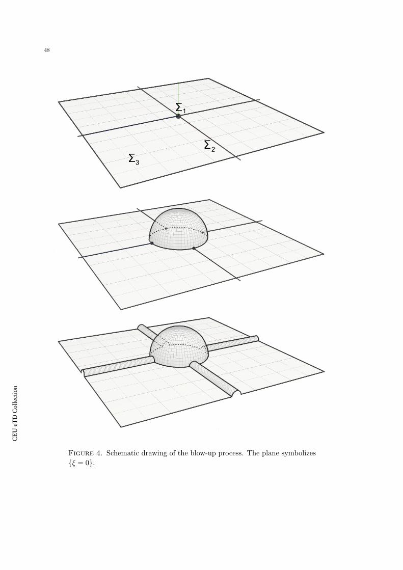
CE
UeT
DC
olle
ctio
n
48
Figure 4. Schematic drawing of the blow-up process. The plane symbolizesξ = 0.

CE
UeT
DC
olle
ctio
n
49
Figure 5. The trees indexing the strata (left) and types of fixed points (right)in the i j = 3 case.
The open set U is simply U = ξ 6= 0 ∼= Hom(IJ,Cn/I). The blow-ups will be denotedby πk : B(k) → B(k−1).
This blow-up process is illustrated in the i j = 3 case on Figure 4. The three picturesshow B(1), B(2) and B(3), respectively; the planes represent the ξ = 0 hyperplane.
Sketch of proof. The only thing not clear is that Σ(k+1)k+1 ⊂ B(k+1) is smooth; this follows
from the fact that normal cone of the (closure of the) rank variety Σk+1 ⊂ Matn×m over Σk
is the cone of the Segre varieties of the projective normal bundle, and the Segre varieties aresmooth, thus the blow-up completely resolves the singularity.
We can further stratify the sets Σ(k)l (and thus B(k)) by distinguishing the points added
in the process of strict transform, that is, those which are in the exceptional divisor Ek.This finer stratification, which is the common refinement of the coarser stratifications at thedifferent levels B(≤k), is best described by pictures. Looking at Figure 4, the first drawing,representing B(1), has 3 strata (not counting U); the second, B(2) has 5; finally, B(3) has7. The strata are indexed by nodes of trees: Figures 5 (left) and 6 shows these trees in thei j = 3 and i j = 4 cases, respectively (the root → ξ 6= 0 edge is missing from thesetrees; it would represent the open stratum U). The (boxed) leaves of the trees index thestrata of the final stratification B(ij).
The blow-up, by definition, replaces the subvariety X we are blowing up by the projec-tive bundle associated to its normal bundle. We can visualize that by imagining that weare moving away from X by an infinitesimal distance, into different directions. From thispoint of view, the strata (the nodes of the trees) enumerate the combinatorial possibilitiesof “travelling” between the subsets of different rank.
The reason why we did this complicated blow-up process is of course the following
Proposition 4.3.5. The rational map sol : B(1) 99K Grµ(J2(n)), with domain of regularityV = U ∪ Σij, extends to a regular (and birational) map sol : B(ij) → Grµ(J2(n)).
Before proving this theorem, let us construct, for all strata (actually for any point in theindeterminacy locus Z = B(ij) − V ), curves γ(t) : C× → V such that limt→0 γ(t) lands in

CE
UeT
DC
olle
ctio
n
50
Figure 6. The tree indexing the strata in the i j = 4 case.
the given strata (is the given point). This is easy to do: Consider the path in the index treefrom the root to the leaf corresponding to the given strata. This path, for example
root→ rk = 1 → rk = 3 → rk = 4 → ξ 6= 0,
describes how we “travel” between the different rank varieties, and thus can be directlytranslated into a curve γ(t), for example in this case (and i j = 5, n− i = 7)
[ ξ(t)·idIJ | α2(t) ] =
t3 1
t3 t
t3 t
t3 t2
t3 0 0 0
works (the whole curve lives over a fixed flag (I, J) ∈ Flij(n)). More formally: If the pathdescribing the strata is
root→ rk = r1 → rk = r2 → · · · → rk = rk → ξ 6= 0,
we put (1, . . . , 1︸ ︷︷ ︸
r1
, t, . . . , t︸ ︷︷ ︸r2−r1
, t2, . . . , t2︸ ︷︷ ︸r3−r2
, . . . , tk−1, . . . , tk−1︸ ︷︷ ︸rk−rk−1
, 0, . . . , 0︸ ︷︷ ︸ij−rk
)on the diagonal of α2(t), and set ξ(t) = tk; the other possibility is that last node is rk = ij,in which case we set ξ(t) = 0. For any given point in the indeterminacy locus Z = B(ij)−V ,we can take a curve which looks like this in a suitable coordinate system. Note that fromthis form, it is very easy to read off the limit
limt→0
sol(γ(t)) ∈ Grµ(J2(n));
in our example it is the subspace of linear functions in J2(n) = (Sym2Cn ⊕ Cn)∨ vanishingon K = (id⊕ q−1
I )(L) ⊂ Sym2Cn ⊕ Cn,
L =
[ 0 0 0 0 ∗ | ∗ ∗ ∗ ∗ 0 0 0 ]⊂ IJ ⊕ (Cn/I),
qI : Cn → Cn/I.

CE
UeT
DC
olle
ctio
n
51
Next, we will extend the above construction, so that not only we can approach any pointz ∈ Z on a curve, but we can approach it from any direction. That is, given a tangent vectorv ∈ TzB(ij) − TzZ, we want a curve γ′(t) : C× → V such that
limt→0
γ′(t) = z andddtγ′(t)
∣∣t=0
= v.
To do that, we modify the existing curves; basically we can “shear” along the directionsparallel to Σ(k)
k . In our running example, α2(t) will become the modified α′2(t)
α′2(t) = Aλ(t)+t·
∗ ∗ ∗ ∗ ∗ ∗∗∗∗∗
+t2 ·
·∗ ∗ ∗ ∗ ∗
∗ ∗ ∗ ∗ ∗∗ ∗∗ ∗
+t3 ·
···
∗ ∗ ∗∗
+t4 ·
····∗ ∗ ∗
ξ′(t) = λ∞t3 + ∗ · t4 Aλ(t) =
λ1
λ2t
λ3t
λ4t2
0 0 0
where we can write are any (constant) numbers into the place of stars, and any nonzeronumbers into the place of λi-s (the small dots in the matrices are only there to indicate todiagonal). Note that we overspecified the tangent vector by one dimension, but that causesno problems.
We can also describe the neighbourhood relationship between the strata. Given a stratumS by its path from the root to a leaf, we can get all the strata S′ for which S ⊂ S
′, that is,those who can degenerate into it (in another words, the neighbouring strata) by taking allthe possible proper subsets of nodes, and closing with a ξ 6= 0 node those which do not endcorrectly (that is, with either maximal rank or ξ 6= 0). This can be seen via induction. Forexample, the neighbours of 1©→ 2©→ 3© (which corresponds to the corner points on thesemisphere in Figure 4) are: 1©→ 2©→ ξ© , 1©→ 3© , 2©→ 3© , 1©→ ξ© , 2©→ ξ© , 3© andξ© (the last one is just open open stratum U). The codimension of a stratum is the length
(number of nodes) of the corresponding path, not counting the ξ© nodes.
Proof of Proposition 4.3.5. We show that the map sol extends from V = B(ij)−Z to B(ij)
as a continuous map (in the complex topology). For this, simply apply Gauss elimination(alternatively, compute the wedge product of the rows) to the “sheared” matrix [ ξ′(t) ·idIJ | α′2(t) ], and observe that its image does not depend on the the numbers substitutedinto the stars (and λi-s) in the limit t→ 0, that is, on the direction we are approaching from.
We also want to show that this limit depends continuously on the point z ∈ Z. Since wehave the GLn symmetry, and also each fixed fiber over (I, J) ∈ Flij has the extra symmetrygiven by the action of G = GL(IJ) × GL(Cn/I) with the strata there being precisely theG-orbits, the only interesting situation is when we degenerate from a larger stratum S′ to asmaller one S. Consider a parametric family of curves γε(t) for which limt=0(γ0(t)) = z ∈ S

CE
UeT
DC
olle
ctio
n
52
and limt=0(γ6=0(t)) ∈ S′; two representative examples of such families are
Ma =
t5 1
t5 t
t5 (t2 + ε1t)t5 (t3 + ε2t)
t5 t4 0
for S = 1©→ 2©→ 3©→ 4©→ 5© and S′ = 1©→ 4©→ 5© ; and
Mb =
t3 + εt2 1
t3 + εt2 t
t3 + εt2 t
t3 + εt2 t2
t3 + εt2 t2 0
for S = 1©→ 3©→ 5© and S′ = 1©→ 3©→ ξ© . It is a straightforward computation withwedge products to show that in such situtations, ε 7→ limt=0(γε(t)) is continuous (there arethree cases, depending on what happens with the last node).
Finally it is an application of the Riemann extension theorem (see eg. [GH78]) that theresulting extended map is holomorphic.
Now we would like to apply Theorem A.3.7 for Mij = B(ij). For this, we have tounderstand the fixed points. This is easy, since fixed points comes in a hierarchy: The mapπk : B(k) → B(k−1) maps the fixed point set Fix(k) to Fix(k−1). Since B(1) is just a projectivebundle, its fixed points are triples (I, J, [l]), where (I, J) ∈ Flij(Cn) is a coordinate flag, andl is a coordinate axis. The blow-up process replaces fixed points by projectivized normalspaces, and thus introduces new fixed points. So a typical fixed points (over an implicitlyspecified fixed flag) looks like this:
α2 =
· · · · · · ·
· · · t · · ·· 1 · · · · ·· · · · · · ·· · · · · t2 ·
, ξ = t3.
The lines in the matrix represent the tangent spaces of the Σ(k)k . Types of fixed points are
indexed by a tree similar to that which indexes the strata, except that we cannot “jumpover” ranks (Figure 5, right). More formally, a fixed point is specified by the following data:
• A coordinate flag (I, J), which we identify with subsets J ⊂ I ⊂ n = 1, 2, . . . , n,where |I| = i and |J | = j;• a natural number 0 ≤ k ≤ i j, specifying the type of the fixed point;• two subsets S ⊂ IJ and R ⊂ n− I, with |S| = |R| = k;• two permutations σ, % ∈ Sk.
A curve tending to the fixed point given by this data is
[α2(t)]ab =ti−1 a = Sσi and b = R%i ,
0 otherwise;ξ(t) =
tk k < i j,0 k = i j;
(distinguishing between two cases for ξ is actually not necessary). The solution over thatfixed point is the space of jets vanishing on K = (IJ − S)⊕ q−1(R).

CE
UeT
DC
olle
ctio
n
53
Remark. The number of fixed points is
#Fix =(n
i
)(i
j
)︸ ︷︷ ︸
the flag
·ij∑k=0
(i jk
)(n− ik
)(k!)2.
An obvious disadvantage of our blow-up method is the combinatorial explosion of the fixedpoints; however, in this particular case, we can simplify a bit and will remove the (k!)2 factorbelow.
Finally, we have to understand the tangent Euler class, that is, the tangent weights of afixed point. As before, this is done inductively, from blow-up to blow-up. We start with thespace Hom(IJ,Cn/I), which has weights
αk − αi − αj : (i, j) ∈ IJ, k /∈ I.
However, to simplify the notation, for a moment consider just any torus representations An
and Bm, m ≥ n, with weights ϕ1, ϕ2, . . . and ψ1, ψ2, . . . , and apply the blow-up process toP[1⊕ Hom(A,B)]. Also, let us assume that R and S are simply the first k coordinates, andthe permutations are trivial. These assumptions are of course not essential, but clarify thepresentation significantly.
We will also use the notation wab = ψb − ϕa for the weights of Hom(A,B). The fixedpoint z(1) ∈ P[1⊕ Hom(A,B)] has tangent weights
N (0) =
0− w11
∪wab − w11 : a 6= 1 or b 6= 1
,
which can be partitioned to the tangent and normal spaces T (1) and N (1) of Σ(1)1 at z(1):
T (1) =wab − w11 : a = 1 xor b = 1
,
N (1) =wab − w11 : a > 1 and b > 1
∪
0− w11
,
where we use ‘xor’ as the standard abbreviation for ‘exclusive or’. The blow-up leaves T (1)
unchanged, and replaces N (1) by L(1) ⊕ Tz(2)PN (1), the line L(1) ⊂ N (1) = N (0)/T (1) beingthe tautological line 〈z(2)〉+T (1). Thus the tangent weights of z(2) are T (1)∪L(1)∪T (2)∪N (2),
L(1) =w22 − w11
T (2) =
(wab − w11)− (w22 − w11) : a = 2 xor b = 2, a ≥ 2, b ≥ 2
=
=wab − w22 : a = 2 xor b = 2, a ≥ 2, b ≥ 2
,
N (2) =
(wab − w11)− (w22 − w11) : a > 2 and b > 2∪
(0− w11)− (w22 − w11)
=
=wab − w22 : a > 2 and b > 2
∪
0− w22
.
At this point, it is easy to spot the pattern, which is illustrated on Figure 7. On the picture,the matrix Hom(A,B) is shown; the arrows denote subtractions of weights.
At the end of the day, the weights of our fixed point will be
T (1) ∪ L(1) ∪ T (2) ∪ L(2) ∪ · · · ∪ T (k) ∪ L(k) ∪N (k).
Note that since in the last blow-up we always select the ξ 6= 0 direction, L(k) = 0 − wkkand N (k) will be simply
N (k) =wab : a > k and b > k
,

CE
UeT
DC
olle
ctio
n
54
Figure 7. The weights of a fixed point. The arrows denote subtractions.
except when k = dim(A), in which case L(k−1) = wkk − wk−1,k−1 and N (k) = 0− wkk.
We can now write down the tangent Euler class at our fixed point x specified by thequadruple x = (S,R, σ, %) (specifying k is superfluous, since k = |S| = |R| = |σ| = |%|). Notethat we use the convention that σ(u) : 1 ≤ u ≤ k = S ⊂ 1, 2, . . . , i j, and similarlyfor % and R.
e(TxB
(n))
=k∏
u=1
[k∏
a=u+1
(wσ(a),%(u) − wσ(u),%(u)) ·∏i/∈S
(wi,%(u) − wσ(u),%(u)) ·
·k∏
b=u+1
(wσ(u),%(b) − wσ(u),%(u)) ·∏j /∈R
(wσ(u),j − wσ(u),%(u))
]·
· (0− wσ(k),%(k)) ·k∏
u=2
(wσ(u),%(u) − wσ(u−1),%(u−1)) ·∏i/∈S
∏j /∈R
wi,j .
We can rewrite this as follows. To simplify the notation, let us introduce the convention thatwσ(k+1),%(k+1) = w0,0 = 0; also, (i, a) ∈
(S2
)means the set of pairs (i, a) ∈ S such that i < a.
e(TxB
(n))
=k∏
u=1
(wσ(u+1),%(u+1) − wσ(u),%(u)) ·
· sgn(σ) ·∏
(i,a)∈(S2)(−ϕa + ϕi) · sgn(%) ·
∏(j,b)∈(R
2)(+ψb − ψj) ·
·∏a∈S
∏i/∈S
(−ϕi + ϕa) ·∏b∈R
∏j /∈R
(+ψj − ψb) ·∏i/∈S
∏j /∈R
(ψj − ϕi).
Since the solution over a fixpoint depends only on S and R, but not on σ and %, we can tryto simplify the sum ∑
σ,%
1e(T(S,R,σ,%)B(n))
.

CE
UeT
DC
olle
ctio
n
55
Lemma 4.3.6. We have∑σ∈Sk
∑%∈Sk
[k∏
u=1
(wσ(u+1),%(u+1) − wσ(u),%(u)) · sgn(σ)sgn(%)
]−1
=
= (−1)k ·
∏(i,a)∈(S
2)(−ϕa + ϕi) ·
∏(j,b)∈(R
2)(+ψb − ψj)∏
i∈S∏j∈R
(ψj − ϕi
) = (−1)k · det
[1
ψj − ϕi
]k×k
.
Remark. The second equality is Cauchy’s double alternant; we won’t actually use that.
Corollary 4.3.7.∑σ,%
1e(T(S,R,σ,%)B(n))
=
=1[
Hom(R,S)]·[Hom(A− S, S)
]·[Hom(R,B −R)
]·[Hom(A− S,B −R)
] =
=1[
Hom(R+ (A− S), S + (B −R)
)] .Remark. Note that the last expression is just the (inverse of the) tangent Euler class ofthe Grassmannian Grn(A⊕B) at the fixed point K = S⊥ ⊕R. The sign (−1)k = (−1)(k
2)ishidden in the term [Hom(R,S)].
Proof of Lemma 4.3.6. We can apply the idea presented in Section A.3.1, and use localizationto prove this identity. Consider the representation Hom(A,B); first blow up the origin (locusof rank 0 matrices), then blow up the locus the rank 1 matrices, and so on. The constructionis very similar what we did before, except that we here started with Hom(A,B) instead ofP(1 ⊕ Hom(A,B)). The method of A.3.1 applied to this this geometric situation proves aformula which is, up to sign and ordering of variables (which does not matter, as the sum issymmetric), is the same as the statement of the Lemma.
More formally, this sequence of blow-ups gives us a chain of identities
E0 :=1∏
i∈A∏j∈B(ψj − ϕi)
= E1 = E2 = · · · = Ek,
where
Er =∑|S|=r
∑|R|=r
∑σ∈SS
∑%∈SR
1D · V1 · V2 ·N
D = wσ(1),%(1) ·(wσ(2),%(2) − wσ(1),%(1)
)· · ·(wσ(r),%(r) − wσ(r−1),%(r−1)
)V1 =
r∏s=1
[r∏
u=s+1
(wσ(u),%(s) − wσ(s),%(s)
)·∏i/∈S
(wi,%(s) − wσ(s),%(s)
)]
V2 =r∏s=1
r∏v=s+1
(wσ(s),%(v) − wσ(s),%(s)
)·∏j /∈R
(wσ(s),j − wσ(s),%(s)
)N =
∏i/∈S
∏j /∈R
(wij − wσ(r),%(r))
wi,j = ψj − ϕi

CE
UeT
DC
olle
ctio
n
56
Note that though these A, B, S, R, etc. are very similar to the previous ones, they areunrelated, local to this proof! The two ends of the chain gives E0 = Ek, which for |A| =|B| = k is equivalent to the lemma.
4.3.2.2. The canonical compactification. It turns out that it is actually easy to under-stand the closure of j(Mij) ⊂ GrµJ2(n) directly. For
(I, J, α2) ∈Hom(I J,Cn/I)→ Flij(n)
=Mij
and (F1, F2) ∈ J2(n,m) (in particular, for m = 1 too) we can rewrite our equations into thesingle equation (F1 + F2)|K = 0 where
K = (id⊕ q−1I )(im(idIJ , α2)
)qI : Cn → Cn/I
In other words, we take the graph graph(α2) ⊂ (I J) ⊕ (Cn/I) of the (linear) map α2 :I J → Cn/I. This gives the map j : Mij → GrµJ2(n)∨ = GrµJ2(n). Clearly, j factorsthrough the bundle of Grassmannians Y = Grij(I J ⊕ Cn/I) → Flij , which is compact,and is embedded into GrµJ2(n); thus the the closure of j(Mij) can be constructed by takingthe closure in Y , and embedding it to GrµJ2(n).
Now the question is, basically, that which linear subspaces arise as limits of graphs? Andthe answer is: ‘all’. For two vector spaces V v and Ww, the image of graph : Hom(V,W ) →Grv(V ⊕W ) is the open Schubert cell in Grv(V ⊕W ). So we have
j(Mij) = Y ⊂ GrµJ (n)
4.3.3. The localization formula. We get the same formula out of both methods:
[Σij ] =∑I∈(n
i)
[Hom(I,Θ)][Hom(I, n− I)]
∑J∈(I
j)
1[Hom(J, I − J)]
∑K∈(IJ+n−I
ij )
[Hom(K,Θ)][Hom(K, (IJ + n− I)−K)]
where, with some abuse of notation, n stands for (α1, . . . , αn), Θ = (θ1, . . . , θm), and thebrackets denote the Euler class of the representation inside (as in [V ] = [0 ⊂ V ] ∈ H∗
G(pt)).Notice that the inner sum is just the localization formula for Σij(IJ+n−I,Θ) (see Section1.3), which we can evaluate as a Schur polynomial, thus
[Σij ] =∑I∈(n
i)
∑J∈(I
j)
s(im)(Θ− I) · s((ij)m−n+i)(Θ− (IJ + n− I))[Hom(I, n− I)] · [Hom(J, I − J)]
And this sum is just calculating the pushforward along π : Flij(n)→ pt (see Corollary A.3.3),resulting in
[Σij ] = π∗s(im)(Θ− I) · s((ij)m−n+i)(Θ− (IJ + n− I))
which is just Ronga’s pushforward formula (Theorem 4.2.1).
We can also evaluate the localization formula using the technique presented in Section3.2. We implemented this method as a computer program (written in Haskell), substitutingrational numbers, and found that it is practical for n, µ ≤ 9: Table 3 shows the running timeson an average personal computer (note that for the cases not marked ‘new’, we actually haveexplicit formulae, see the next two sections). Using floating point arithmetic one can gainseveral orders of magnitude in speed, which may further extend the range where computer

CE
UeT
DC
olle
ctio
n
57
calculations are possible with this method (which has the advantage of computing them =∞case directly; see Figure 3 on page 27).
4.4. Explicit formulae for the coefficients
In this (and part of the next) section we present the results of our article [FK06] jointwith Laszlo Feher. It is based on the idea of restricting Σij to Σk (in the sense of Section1.4) for k ≤ i, though this is implicit in the argument we present here.
Recall that
Σij(V,W ) =
(α1, α2) ∈ J2(V,W ) = Hom(V,W )⊕ Hom(Sym2V,W )
: corank(α1) = i, and α2 ∈ Σ•,j(ker(α1), coker(α1))
where α2 : Sym2(ker(α1))→ coker(α1) is the natural map induced by α2, and
Σ•,j(A,B) =ϕ ∈ Hom(Sym2A,B) : corank(curry(ϕ)) = j
.
singularity new µ = i+ i j n running time # of terms
Σ2,1 4 4 negligible 75 0.3 seconds 176 2 seconds 337 10 seconds 578 45 seconds 90
Σ2,2 5 5 1 second 316 7 seconds 647 40 seconds 1178 3.5 minutes 199
Σ3,1 6 6 31 seconds 1107 7 minutes 2778 not measured 5929 not measured 11376 5.5 minutes 2307 105 minutes 689
Σ3,2 ? 8 8 several hours – one day 17336 2.5 minutes 156
Σ3,3 ? 9 9 one day – few days 32226 34 seconds 1077 25 minutes 450
Σ4,1 8 8 several hours 13936 11 minutes 269
Σ4,2 ? 11 11 out of reach ?
Table 3. Running times for computing TpΣij (n,∞) using the method of Sec-tion 3.2. Where times are approximate, the calculations were ran on different(faster) computer, and not exactly measured.

CE
UeT
DC
olle
ctio
n
58
Here curry denotes the (restriction of the) natural isomorphism
curry : Hom(A⊗B,C) ∼−−→ Hom(A,Hom(B,C)).
Remark. In the following, we will either assume that m ≥ n, or define corank as the sourcecorank, that is, corank(ϕ : Cn → Cm) = n − rank(ϕ), even if m < n. Note that though thistheory works for m < n, from the Thom series point of view it is enough to consider them n case.
It follows directly from this definition that Σij(n,m) is empty if n < i and it is particularlysimple for n = i:
Σij(Ai, Bm−n+i) = 0 × Σ•,j(A,B) ⊂ J2(A,B);
which means that its class is a product:[Σij(Ai, Bm−n+i)
]= e(Hom(A,B)) ·
[Σ•,j(A,B)
].
We can exploit the simplicity of these cases because the stability : The Thom polynomialactually depends only on the (formal) difference B − A, that is, there exists a universalpolynomial in the formal variables ci
Tp(r) ∈ Z[c1, c2, c3, . . . ]
such that the classes [Σ(An, Bm)] can be obtained by the specialization %A,BTp(m−n), where
%A,B : Z[c1, c2, c3, . . . ]→ H∗G(A)⊗H∗
G(B)
ci 7→ cGi (B −A)
This notation is a bit strange (the correct interpretation is that A and B are G-equivariantvector bundles over some base manifold M), so let us work with the formal version instead:
%n,m : Z[c1, c2, c3, . . . ]→ Z[a1, a2, . . . an; b1, b2, . . . , bm]
which is defined by the equation∞∑k=0
%n,m(ci)ti =1 +
∑mj=1 bjt
j
1 +∑n
i=1 aiti
with t being a formal variable. (This corresponds to let A and B be the standard GLnresp. GLm representations, viewed as GLn × GLm-equivariant vector bundles over the point;ai and bj are then the equivariant Chern classes of A resp. B).
We will use the following well-known properties of the map %n,m.
Proposition 4.4.1.
(i) ker(%n,m) is spanned (over Z) by the Schur polynomials sλ(c) with (n+1)(m+1) ⊂ λ;
(ii) im(%n,m) is spanned by the images of the Schur polynomials sλ(c) with (n+1)(m+1) 6⊂λ;
(iii) Suppose that nm ⊂ λ but (n+ 1)(m+1) 6⊂ λ; that is, λ has the form λ = (nm + β, α)with `(β) ≤ m and `(α) = α1 ≤ n (see Figure 8). Then we have to so calledfactorization formula
%n,m(sλ(c)) = s(nm)(b− a) sα(−a) sβ(b).
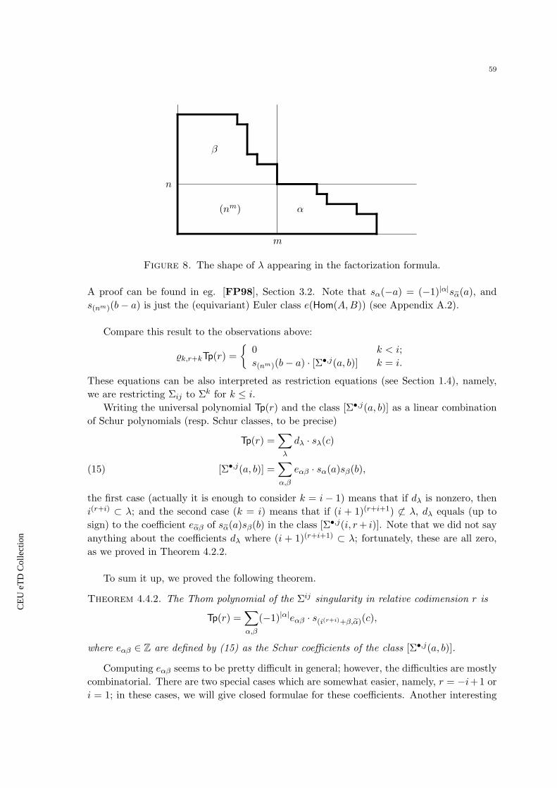
CE
UeT
DC
olle
ctio
n
59
n
m
(nm)
β
α
Figure 8. The shape of λ appearing in the factorization formula.
A proof can be found in eg. [FP98], Section 3.2. Note that sα(−a) = (−1)|α|seα(a), ands(nm)(b− a) is just the (equivariant) Euler class e(Hom(A,B)) (see Appendix A.2).
Compare this result to the observations above:
%k,r+kTp(r) =
0 k < i;s(nm)(b− a) · [Σ•,j(a, b)] k = i.
These equations can be also interpreted as restriction equations (see Section 1.4), namely,we are restricting Σij to Σk for k ≤ i.
Writing the universal polynomial Tp(r) and the class [Σ•,j(a, b)] as a linear combinationof Schur polynomials (resp. Schur classes, to be precise)
Tp(r) =∑λ
dλ · sλ(c)
[Σ•,j(a, b)] =∑α,β
eαβ · sα(a)sβ(b),(15)
the first case (actually it is enough to consider k = i− 1) means that if dλ is nonzero, theni(r+i) ⊂ λ; and the second case (k = i) means that if (i + 1)(r+i+1) 6⊂ λ, dλ equals (up tosign) to the coefficient eeαβ of seα(a)sβ(b) in the class [Σ•,j(i, r+ i)]. Note that we did not sayanything about the coefficients dλ where (i + 1)(r+i+1) ⊂ λ; fortunately, these are all zero,as we proved in Theorem 4.2.2.
To sum it up, we proved the following theorem.
Theorem 4.4.2. The Thom polynomial of the Σij singularity in relative codimension r is
Tp(r) =∑α,β
(−1)|α|eαβ · s(i(r+i)+β,eα)(c),
where eαβ ∈ Z are defined by (15) as the Schur coefficients of the class [Σ•,j(a, b)].
Computing eαβ seems to be pretty difficult in general; however, the difficulties are mostlycombinatorial. There are two special cases which are somewhat easier, namely, r = −i+1 ori = 1; in these cases, we will give closed formulae for these coefficients. Another interesting

CE
UeT
DC
olle
ctio
n
60
case is j = i, when we can give a nice combinatorial interpretation of the coefficients, butthe problem of giving formulae or an enumerative recipe to compute them is unsolved. Wecan compute the case i = j = 2, however.
Theorem 4.4.3. Let π : Grj(Ai)→ pt denote the projection map from the Grassmannian ofj-planes in A to the one-point space, and J j be the tautological (equivariant) vector bundleover Grj(A). Then [
Σ•,j(Ai, Br+i)]
= π∗e(Hom((π∗A) J, π∗B),(16)
where e, as usual, is the equivariant Euler class, with the group GL(A) × GL(B) actingnaturally.
Proof (compare with [LP00], Section 3). Consider the diagram
Hom(A⊗A,B) = A∨⊗A∨⊗B σ−→ J∨⊗A∨⊗B −→ J∨⊗J∨⊗By yqA yqJ
Hom(∧2A,B) = ∧2A∨⊗B −→ ∧2J∨⊗B
over a fixed J ∈ Grj(A). Note that Hom(Sym2A,B) ∼= ker(qA); thus any ϕ ∈ Hom(Sym2A,B)gives us a section σ(ϕ) of the vector bundle ker(qJ)→ Grj(A). Combining these for differentϕ’s, we get a section σ of the bundle
ker(qJ)→ Grj(A)× Hom(Sym2A,B).
Observe that the image of the map pr2 restricted to the zero locus Z of the section σ
pr2|Z : Z = σ−10 ⊂ ker(qJ)
→ Hom(Sym2A,B)
is Σ•,j , and it’s one-to-one on Σ•,j ; thus the locus Z is a resolution of Σ•,j (it is clear that σis transversal to the zero section, thus Z is smooth). From that, it follows that
[Σ•,j ] = π∗e(ker(qJ));
but of course, ker(qJ) ∼= Hom(A J,B).
Naturally, one would try to apply the pushforward formula (Theorem A.4.1) to evaluate(16). For this, we have to separate the “variable” J ; the first step is
π∗e(Hom(A J, B) =∑
λ⊂(r+i)(ij)
(−1)|λ|seλ(B) · π∗sλ(A J).
However, the problem of expanding sλ(A J) into
sλ(A J) =∑ϕ,ψ
fϕψ · sϕ(A)sψ(J)(17)
is unsolved in general. This question belongs to a larger family of similar expansion problems,most of which is unsolved. There are some tractable special cases, though:
(a) j = 1: in this case, A J = A ⊗ J , and the coefficients fϕψ were computed byLascoux in [Las78] (Lemma A.2.8);
(b) r + i = 1: in this case, λ = (1k) is special; s(1k) is just the kth Chern class; for thetop Chern class, a formula is proved in [LP00];

CE
UeT
DC
olle
ctio
n
61
(c) i = j: in this case, A J = Sym2A; this is unsolved, but we can compute thesmallest nontrivial case i = j = 2, see Section 4.5.2. Note that in this case π
is trivial, so there is no pushforward; thus the coefficients in the Thom series areexactly the same as the coefficients fϕψ!
Nonetheless, we will not use Theorem 4.4.3 directly for cases (a) and (b), but handle themwith different approaches. Case (c) serves as a motivation: It shows that the coefficients ofthe Thom polynomials have very rich combinatorics. We find this very important, so let usrepeat it as a theorem:
Theorem 4.4.4. The Thom series of the Σii singularity is Ts =∑fν±rsν±, where fν± is the
coefficient of sν+(Ai) in the expansion of sν−(Sym2Ai). (Note that in this chapter we use the‘shifted base line’ (m− n+ i, n− i), cf. Figure 3).
Next, let us state two theorems about the cases (a) and (b).
Theorem 4.4.5. [Σ•,j(Ai, L1)] = 2j ·sbje(A∨ ⊗√L) where bje = (j, j − 1, . . . , 2, 1).
Remark. Note that the line bundle L has no square root, so the formula above should beunderstood formally: the only Chern root of
√L is β/2 where β = β1 is the Chern root of
L, and then the Chern roots of A∨ ⊗√L are −α1 + β/2, . . . ,−αn + β/2.
Proof. Notice that the elements of Hom(Sym2Ci,C) can be identified with symmetric i × imatrices and then the ‘curried corank’ becomes simply corank, so the class in question is givenby the twisted symmetric degeneracy locus formula ([HT84], [JLP82], [Pra90], [Ful96]).A general explanation of twisting can be found in [FNR05].
Theorem 4.4.6. [Σ•,1(Ai, Br+i)] = ci(r+i−1)+1(A∨ ⊗B −A).
Proof. The codimension of Σ•,1(An, Bm) ⊂ Hom(Sym2A,B) is mn − n + 1, which equalsto the codimension of Σ1(A,A∨ ⊗ B) ⊂ Hom(A,A∨ ⊗ B) = Hom(A ⊗ A,B); so—exactlyas noted in [LP00], where a similar degeneracy locus problem is considered—we are in thesituation of the Giambelli-Thom-Porteous formula, since Σ•,1(An, Bm) is just the transversalintersection Σ1(A,A∨ ⊗W ) ∩ Hom(Sym2A,B):[
Σ•,1(An, Bm)]
= [Σ1(A,A∨ ⊗W )] = cmn−n+1(A∨ ⊗B −A).
4.5. Combinatorics
In this section we will deal with the combinatorics of the special cases mentioned above.
4.5.1. The coefficients for Σi,1. We will need the following statements of LemmaA.2.8:
Lemma ([Las78]). Denote by Eλ/µ(n) the determinant
Eλ/µ(n) = det
[(λi + n− iµj + n− j
)]i,j∈n×n
.

CE
UeT
DC
olle
ctio
n
62
(1) Let An and Bm be an n-dimensional and a m-dimensional (equivariant) vectorbundle, respectively. Then∑
k
ck(A⊗B) =∑
µ⊂λ⊂mn
Eλ/µ(n)sµ(A)seλ(B)
(2) Furthermore, if L is a line bundle and λ is partition with `(λ) ≤ n, then
sλ(A⊗ L) =∑µ⊂λ
Eλ/µ(n)·c1(L)|λ|−|µ| ·sµ(A)
Remark. Our notation Eλ/µ(n) is motivated by the following formula. Suppose that n ≥`(λ), `(µ) (if this is not the case, one should take (λ1, . . . , λn) and (µ1, . . . , µn) instead of λand µ in the RHS); then
Eλ/µ(n) = sλ/µ
(1,
12!,
13!,
14!, . . .
)·∏
(i,j)∈λ/µ
(n+ i− j),
where we substitute 1/k! for the kth elementary symmetric polynomial in the (Jacobi-Trudiexpansion of the) skew Schur polynomial sλ/µ (this is called exponential specialization in thesymmetric polynomial literature, see eg. [Sta99]). The proof of the formula is a straightfor-ward computation (one observes that in the expansion of the determinant Eλ/µ(n) each termis the polynomial
∏(n+ i− j) up to a scalar). An important corollary is that Eλ/µ(n) = 0
if µ 6⊂ λ.
The lemma, together with Theorem 4.4.5 immediately implies the following
Theorem 4.5.1. The Thom polynomial of the second order Thom-Boardman singularityΣij(−i+ 1) in relative codimension r = −i = 1 is[
Σij(−i+ 1)]
=∑µ⊂bje
2|µ|−j(j−1)/2 · Ebje/µ(i) · s(d−|µ|,eµ)
where bje is the ‘stairway’ partition bje = (j, j − 1, . . . , 2, 1) and
d = codim Σij(−i+ 1) = i+(j+12
).
Remark. This is the smallest relative codimension where the singularity appears at all. Inthe Thom series language, this theorem calculates the “lowest degree” part of the Thomseries.
Similarly, Theorem 4.4.6 leads to
Theorem 4.5.2. Using the shorthand notation h = r + i,[Σi,1(r)
]=
∑(λ,µ)∈K
s(ih+λ,µ) ·∑
x∈0,1`(µ)
Eeλ/(µ−x)e(i)
where x runs over the 0-1 sequences of length `(µ), and
K =
(λ, µ) : λ ⊂ ih, µ1 ≤ i, |λ|+ |µ| = ih− i+ 1, and µ− x is a valid partition.
Proof. According to Theorem 4.4.2, to express [Σi,1] all we have to do is to expand theformula cih−i+1(A∨ ⊗B −A) into linear combination of products of Schur polynomials. Forthe sake of convenience, we calculate the total Chern class∑
m≥0
cm(A∨ ⊗B −A) =
∑k≥0
ck(A∨ ⊗B)
·∑l≥0
cl(−A)
.

CE
UeT
DC
olle
ctio
n
63
Using the Lemma, the Pieri formula, and
c(−A) =∑l≥0
cl(−A) =∑k≥0
(−1)ksk(A),
we will get
c(A∨ ⊗B −A) =∑
µ⊂λ⊂ih
∑x∈0,1l(µ)
(−1)|µ+x|Eeλ/eµ(i) · s(µ+x)e(A)sλ(B),
where the second sum runs over 0-1 sequences such that µ+x is a valid partition. From thisthe theorem follows directly, using the fact that Eλ/µ(k) = 0 if µ 6⊂ λ and k ≥ `(λ), `(µ).
Note that in both cases, the Thom polynomial is a nonnegative linear combination ofSchur polynomials. The same is true in general, for any Thom polynomial: This was con-jectured by the author (based on numerical evidence), and independently by Pragacz; andthen proved in [PW07a, PW07b].
With some work, we can get a more elegant formula. Introduce the notationsn
k
:=
k∑j=0
(n
j
)and Fλ/µ(n) := det
[λk + n− kµl + n− l
]k,l∈n×n
.
Note that the numbersnk
also form a Pascal-like triangle:
11 2
1 3 41 4 7 8
1 5 11 15 161 6 16 26 31 32
Theorem 4.5.3.
[Σi,1(r)] =∑
(ν,µ)∈K
Fν/µ(i) · s(ih+eν,eµ)(18)
where K = (ν, µ) : ν ⊂ hi, `(µ) ≤ i, and |ν| − |µ| = i− 1.
Proof. According to Theorem 4.5.2, the coefficient aν,µ of s(ih+eν,eµ) is a sum, which we canrewrite as follows:
aν,µ =∑
x∈0,1µ1
Eν/(eµ−x)e(i) =µ1∑
α1=µ2
µ2∑α2=µ3
· · ·µi∑
αi=0
Eν/α(i)
Expanding the determinant Eν/α(i) and rearranging the sums yields
aν,µ = det
[νk + i− kµl + i− l
−
νk + i− kµ(l+1) + i− (l + 1)
]k,l∈i×i
Observe that aν,µ is of the form det(A−B) where
Bk,l =Ak,l+1 if l < n
0 if l = n
It is an easy exercise then to prove that in such a situation det(A+ βB) = det(A) holds forany β ∈ C.

CE
UeT
DC
olle
ctio
n
64
Note that in the formula (18), the coefficients are manifestly independent of r = m− n;thus what we got here is actually a closed formula for the Thom series:
Corollary 4.5.4. The Thom series of the Σi,1 singularity is
Ts(Σi,1) =∑ν±∈K
Fν−/ν+(i) · rsν±
where
K =
(ν+, ν−) : `(ν+) = `(ν−) = i, |ν−| − |ν+| = i− 1.
Note that with some abuse of notation, here we allow ν+ and ν− to be padded with zeros.
Example 4.5.5. Specializing for Σ21,
Ts(Σ21)] =∑K
(a+ 1d+ 1
b
c
−a+ 1c
b
d+ 1
)· rs(d,c,−b,−a)
where K is the set of quadruples
K = (a, b, c, d) ∈ N4 : 0 ≤ b ≤ a, 0 ≤ c ≤ d, c+ d = a+ b− 1.
4.5.2. The coefficients for Σ22. According to Theorem 4.4.4, the coefficients in theThom series of Σ22 are the same as the coefficients in the expansion
s(a,b,c)(2x, x+ y, 2y) =∑r
d(M−r,r)(a,b,c) · s(M−r,r)(x, y),(19)
where M = a+ b+ c. In this section, we derive a formula for these numbers.
By definition,
s(a,b,c)(2x, 2y, x+ y) =−1
2(x− y)3
∣∣∣∣∣∣(2x)a+2 (2x)b+1 (2x)c
(2y)a+2 (2y)b+1 (2y)c
(x+ y)a+2 (x+ y)b+1 (x+ y)c
∣∣∣∣∣∣Expanding the determinant by the last row, we get
−12(x− y)2
(2b+c+1sa+2
1 s(b,c) − 2a+c+2sb+11 s(a+1,c) + 2a+b+3sc1s(a+1,b+1)
),
using the notational convention that s1 = s1(x, y) = x + y and s(a,b) = s(a,b)(x, y). One(x− y) factor vanishes from the denominator, since the definition of s(n,k) contains that.
First, let us compute the subexpressions of the form sn1s(b,c). For this, recall the fact that
(x+ y)n = cn1 = sn1 =bn/2c∑i=0
T(n−i,i)s(n−i,i),
where
T(n−i,i) =(n
i
)−(
n
i− 1
)= the Catalan triangle
= number of standard Young tableaux of shape (n− i, i).

CE
UeT
DC
olle
ctio
n
65
We will need the Littlewood-Richardson rule for this very special case:
s(a,b)s(p,q) =min(a−b,p−q)∑
i=0
s(a+p−i,b+q+i).
Let us start.
sn1s(b,c) =bn/2c∑i=0
T(n−i,i)s(n−i,i)s(b,c) =bn/2c∑i=0
T(n−i,i)
min(n−2i,b−c)∑j=0
s(n+b−i−j,c+i+j)
Substituting k = i+ j:
=bn/2c∑i=0
T(n−i,i)
min(n−i,b−c+i)∑k=i
s(n+b−k,c+k) =b−c+b(n−b+c)/2c∑
k=0
s(n+b−k,c+k)
min(k,n−k)∑i=max(0,k−b+c)
T(n−i,i) =
=b−c+b(n−b+c)/2c∑
k=0
s(n+b−k,c+k)
[(n
min(k, n− k)
)−(
n
k − b+ c− 1
)]=
=b−c+b(n−b+c)/2c∑
k=0
s(n+b−k,c+k)
[(n
k
)−(
n
k − b+ c− 1
)]since the inner sum is telescopic. Note that the last sum could start from (−∞), and if wedeclare s(b<c) to be zero, then it could stop at (+∞). We can rephrase this as follows: Thecoefficient of s(n+p+q−l,l) in sn1 ·s(p,q) is
coefficient of s(n+p+q−l,l) in sn1 · sp,q =(
n
l − q
)−(
n
l − p− 1
).
Thus we have
s(a,b,c)(2x, x+ y, 2y) =
=−1
(x− y)2(2b+cca+2
1 sb,c − 2a+c+1cb+11 sa+1,c + 2a+b+2cc1sa+1,b+1
)=
=−1
(x− y)2
b(M+2)/2c∑k=0
s(M+2−k,k)
[2b+c
(a+ 2k − c
)− 2b+c
(a+ 2
k − b− 1
)− 2a+c+1
(b+ 1k − c
)+(20)
+2a+c+1
(b+ 1
k − a− 2
)+ 2a+b+2
(c
k − b− 1
)− 2a+b+2
(c
k − a− 2
)].
What remains is to factor the term (x− y)2 out of the expression above. To do this, letus introduce some notations: Let n be fixed, and m = bn/2c; furthermore,
a(n) = (a0, a1, . . . , am) ∈ Z(m+1)
b(n+2) = (b0, b1, . . . , bm+1) ∈ Z(m+2)
s(n) = (s(n), s(n−1,1), s(n−2,2), . . . ) ∈ Z[x, y](m+1)
〈a(n), s(n)〉 =∑i
ais(n−i,i) ∈ Z[x, y]
k(n) = (n+ 1, n− 1, n− 3, . . . , n+ 1− 2m) ∈ N(m+1)
k(n+2) = (n+ 3, n+ 1, n− 1, n− 3, . . . , n+ 1− 2m) ∈ N(m+2)

CE
UeT
DC
olle
ctio
n
66
Then it is a straightforward computation to show that
(x− y)2 · 〈a(n), s(n)〉 = (s(2) − 3s(1,1)) · 〈a(n), s(n)〉 = 〈A(n)a(n), s(n+2)〉
where the matrix A(n) ∈ Mat(m+2)×(m+1) is defined as
A(n) =
1−2 11 −2 1
1 −2 1. . . . . . . . .
1 −2 11 xn
where xn = −3 + (n mod 2)
Proposition 4.5.6. b(n+2) ∈ im(A(n)) if and only if 〈k(n+2), b(n+2)〉 = 0.
Proof. k(n+2) generates ker([A(n)]†).
In this case, we have a left pseudo-inverse J (n) ∈ Mat(m+1)×(m+2):
J (n) = [A(n)]−1 =
1 02 1 03 2 1 04 3 2 1 0...
. . . . . . . . ....
m · · · 3 2 1 0 0m+ 1 · · · 4 3 2 1 0
With this, we can complete the computation: Just multiply the expansion vector of (20)
by the matrix J (M). This results in
Theorem 4.5.7. The coefficient of s(M−r,r)(x+y) in (the expansion of) s(a,b,c)(2x, x+y, 2y)is
d(M−r,r)(a,b,c) =−
r∑k=0
(r + 1− k) ·[2b+c
(a+ 2k − c
)− 2b+c
(a+ 2
k − b− 1
)− 2a+c+1
(b+ 1k − c
)+(21)
+2a+c+1
(b+ 1
k − a− 2
)+ 2a+b+2
(c
k − b− 1
)− 2a+b+2
(c
k − a− 2
)].
Recall the following notation introduced in the previous section:n
k
=
k∑j=0
(n
j
).
With this notation, we can simplify a bit the type of sums appearing in (21):
Lemma 4.5.8. For n, r, b ∈ N,r∑
k=0
(r + 1− k)(
n
k − b
)=
r−b∑j=0
n
j
.
Proof. Straightforward.

CE
UeT
DC
olle
ctio
n
67
Corollary 4.5.9.
d(M−r,r)(a,b,c) =− 2b+c
b∑j=c
a+ 2r − j
+ 2a+c+1
a+1∑j=c
b+ 1r − j
− 2a+b+2
a+1∑j=b+1
c
r − j
.(22)
Putting together with Theorem 4.4.4:
Theorem 4.5.10. The Thom series of the Σ22 singularity is
Ts(Σ22) =∑ν±
dν+ν− · rsν± ,
where ν± runs over the pairs of partitions such that `(ν+) ≤ 2, `(ν−) ≤ 3, and |ν+| = |ν−|,and dν+ν− is defined by (22) above.
Remark. Compare this formula with Example 4.5.5, which gives a formula for Σ21. It isintriguing that both contain the numbers
nk
; however, the connection between the two is
not at all clear.

CE
UeT
DC
olle
ctio
n
Chapter 5. Third order - A3
In the last chapter, we sketch how to modify the “blow-up method” of Section 4.3.2.1 towork with the A3 (or Σ111) singularity. We believe it can be also adapted to other (small)singularities, eg. A4, Σ211, Σ221; however, the computations did not work out yet. For thisreason, some of the statements are presented in more generality than needed for the A3 case.
We find it possible that this method could even work for all third order Thom-Boardmansingularities (Σijk), however this only of theoretical interest, since the vast number of fixedpoints (or possibly fixed components) make any computation inpractical already for smallcases. A very rough estimation of the number of fixed points is (µ!)2, for the smallest casen = µ; so for example Σ321, with µ = 13 seems to be completely out of reach with thismethod, while Σ221, with µ = 8, is around the limits of present-day personal computers.
5.1. The probe model for Σijk
Recall Porteous’ probe model (we concentrate on the d = 3 case here):
Proposition 5.1.1 ([Por83]). F ∈ J3(n,m) belongs to the Thom-Boardman class Σijk ifthere exists a probe (α, β, γ) ∈ Pijk = J 3 (i, n)× J 2 (j, i)× J 1 (k, j) such that
0 = d(F α)|00 = d(d(F α) β)|00 = d(d(d(F α) β) γ)|0,
and no such probe exists for higher Boardman indices.
We can rewrite these equations to a linear form, using the tensor notation of AppendixA.1. The expansion of third, most complicated equation is shown in Figure 9.
Proposition 5.1.2 ([Por83]). If (α, β, γ) is a good probe for F , then so is (α′, β′, γ′) definedby the commutative diagram
Cn α←− Ci β←− Cj γ←− Ck∥∥∥ yϕ yψ yχCn α′←−− Ci β′←−− Cj γ′←−− Ck
(23)
where (ϕ,ψ, χ) ∈ Gijk = Diff3(i)× Diff2(j)× Diff1(k) are jets of biholomorphisms.
Proposition 5.1.3. The moduli space Mijk of the probes is, set-theoretically,
Mijk =
(I, J,K, α2, α3, β2) : (I, J,K) ∈ Flijk(Cn)
, α2 ∈ Hom(IJ, Cn/I), α3 ∈ Hom(IJK, Cn/I)
, β2 ∈ Hom(JK, I/J)
Proof. Apply Gauss elimination to the equations written in a matrix form. The proof showsthat β2 should be probably called ‘alpha’ too, however, we think that would be equallyconfusing.
68

CE
UeT
DC
olle
ctio
n
69
Figure 9. The 7 terms of the expression d(d(d(F α) β) γ)|0.
These spaces are remarkably subtle. At first sight, they look quite simple: They are fiberbundles (actually, towers of fiber bundles), and the fibers are vector spaces. But they are notholomorphic vector bundles, at least not with the complex structure defined by requiring thequotient map Pijk →Mijk to be analytic.
However, one aspect of the vector bundle structure (ofMij) survives the generalization,namely, a C×-action, generalizing the multiplication by scalars. Suppose we multiply α2 bya nonzero scalar ω ∈ C×; now, there is only way to extend this to an action of C× on thespace of probes P which is compatible with the factor map q : P →M, which is to multiplythe degree d components by ωd−1:
Proposition 5.1.4. Let C× act on the space of probes
PI =d∏
k=1
J d+1−k(ik, ik−1)
by the formula
ω : J d+1−k(ik, ik−1) → J d+1−k(ik, ik−1)(β1, β2, β3, . . . , βd+1−k
)7→
(β1, ωβ2, ω
2β3, . . . , ωd−kβd+1−k
)

CE
UeT
DC
olle
ctio
n
70
This action induces a well-defined action on MI = PI/∼, via the formula
ω · x = qI(ω · y), y ∈ q−1I (x).
Note that im(α1) ⊃ im(α1 β1) ⊃ im(α1 β1 γ1) ⊃ . . . define a fibrationMI → FlI(Cn),and we act on the fibers (the action is trivial on FlI).
Lemma 5.1.5 (Boardman). The codimension of Σijk is
codim(Σijk) = (m− n+ i)µijk − (i− j)µjk − (j − k)k,
where
µijk = i+ i j + i j kµjk = j + j k.
Remark. This codimension formula has a straightforward generalization for higher orderThom-Boardman singularities, but we will not need the general case.
5.2. Morin singularities
The case i = j = k = · · · = 1, called Morin singularities, deserves special attention. Thesewere studied in [BSz06, Ber08], and it was that work where the idea of applying equivariantlocalization to the computation of Thom polynomials first appeared. This was also the casewhich motivated a large part of our work: The original goal was to find an alternate (andpossibly more general) approach to the compactification of these moduli spaces, since eventhough they were able to derive iterated residue formulae for the Thom polynomials of Adfor d ≤ 6, the spaces appearing in the process are not very well understood geometrically.Unfortunately, this program didn’t really work, since the geometry is indeed intricate.
Theorem 5.2.1 ([BSz06], [Gaf83]). For Ad = Σ11...1, the moduli of probes (which in thisparticular case is also called the moduli of test curves) is the quotient
Md = J d (1, n)/Diffd(1),
that is, jets of curves in Cn up to reparameterization. The solutions in Jd(n,m) for a fixedtest curve γ ∈ J d (1, n) are
sol(γ) =F ∈ Jd(n,m) : F γ = 0
.
Proof. Recall Mather’s theorem: Two germs are K-equivalent if and only of their idealsare taken into each other by a diffeomorphism germ. The protype ideal for Ad is Id =(x2, x3, . . . , xn) Jd(n). Suppose we have a germ F = (f1, . . . , fm) of type Ad: Then thereexists a diffeomorhism germ ϕ ∈ Diffd(n) such that the ideal (f1 ϕ, . . . , fm ϕ) is Id; thusF γ = 0 for γ(t) = ϕ(t · dx1). Conversely, suppose that F γ = 0; for any γ there is aψ ∈ Diffd(n) such that ψ γ = (t 7→ tdx1), that is, (f1 ψ−1, . . . , fm ψ−1) ⊂ Id.
Remark. It is not hard to see this from Porteous’ model; in fact, we don’t even need theBoardman indices i = j = k = . . . to be exactly 1, we only need them to be equal. Lookat diagram (23): For any fixed ϕ ∈ Diffd(i), there is a unique ψ ∈ Diffd−1(i), χ ∈ Diffd−2(i),etc. such that β′ = γ′ = · · · = id : Ci → Ci; thus Piii.../Giii... = J d (i, n)/Diffd(i). Dimensioncalculation shows that there are no further ambiguities in the probes, soMiii... = Piii.../Giii....

CE
UeT
DC
olle
ctio
n
71
We adopt the notation x, u, v, w, . . . ∈ Cn for the components of our test curve:
γ ∈ J d (1, n)
γ(t) = xt+ ut2 + vt3 + wt4 + · · ·
(these corresponds to α1, α2, α3, . . . in the old notation), and A,B,C,D, . . . for the compo-nents of the singularity (which corresponds to F1, F2, F3, . . . in the old notation). Note thatx 6= 0. Then the equations can be written as
0 = Ax
0 = Au+Bxx
0 = Av + 2Bux+ Cxxx
0 = Aw +Buu+ 2Bvx+ 3Cuxx+Dxxxx...
In general, the terms in the dth equations correspond to partitions of d, and the coeffi-cients (which are mostly irrelevant) are the number of automorphisms of the partition (see[BSz06]). Note that there are at least two different conventions for the coordinatization ofthe symmetric tensors B,C,D, . . . ; the other convention results in different coefficients.
We can represent the group Diffd(1) and its action on the space of test curves withmatrices: Denoting the components of a diffeomorphism jet by (α, β, γ, . . . ), using the d = 4case as an example, the action reduces to the matrix multiplication
α
β α2
γ 2αβ α3
δ 2αγ + β2 3α2β α4
·x1 x2 . . . xnu1 u2 . . . unv1 v2 . . . vnw1 w2 . . . wn
=
x′1 x′2 . . . x′nu′1 u′2 . . . u′nv′1 v′2 . . . v′nw′1 w′2 . . . w′n
Note that Diffd(1) acts on J d (1, n) on the left, while GLn acts on the right; thus, these
two actions commute, and GLn also acts on the quotient space Md = J d (1, n)/Diffd(1).
Theorem 5.2.2 (cf. [BSz06], Prop. 4.4). For any test curve (x, u, v, w, . . . ) with xi 6= 0,there is a unique diffeomorphism jet (α, β, γ, . . . ) ∈ Diffd(1) such that for the new curve(x′, u′, v′, w′, . . . ) we have x′i = 1, and u′i = v′i = w′i = · · · = 0.
Proof. This is basically the Lagrange inversion theorem. The unique (α, β, . . . ) can be writtendown explicitly:
α =1xi
β =−uix3i
γ =2u2
i − xivix5i
δ =5xiuivi − 5u3
i − x2iwi
x7i...
The coefficients in these formulae are Sloane’s A111785 [OEIS].

CE
UeT
DC
olle
ctio
n
72
This theorem gives us an atlas on the moduli space of test curves: The charts are xi = 1,ui = vi = wi = · · · = 0 for 1 ≤ i ≤ n, and the transition functions are compositions of twodiffemorphisms. The atlas gives a down-the-earth definition of the complex structure on themoduli space of test curves Md = J d (1, n)/Diffd(1).
Example. Consider the transition function from ith chart to the jth chart. The notationwill be such that xi = 1, ui = vi = wi = 0 and x′j = 1, u′j = v′j = w′j = 0, and k 6= i, j.These transition functions can be also written down explicitly:
x′i = 1xj
x′k = xkxj
u′i = −uj
x3j
u′k = ukxj−xkuj
x3j
v′i =−vjxj+2u2
j
x5j
v′k =vkx
2j−2ukujxj−xkvjxj+2xku
2j
x5j
w′i =−wjx
2j+5vjujxj−5u2
j
x7j
w′k =wkx
3j−3vkujx
2j−2ukvjx
2j+5uku
2jxj−xkwjx
2j+5xkvjujxj−5xku
3j
x7j
Remark. Note that these expressions for α, β, . . . are homogeneous with respect to twodifferent grading : The first one is the standard grading deg(x) = deg(u) = deg(v) = · · · = 1;and the second one is deg(x) = 0, deg(u) = 1, deg(v) = 2, deg(w) = 3, etc. The transitionfunctions are also homogeneous wrt. the second grading; this observation motivated our C×
action.
Theorem 5.2.3. The C× action on J d (1, n) defined by
ω · (x, u, v, w, . . . ) = (x, ωu, ω2v, ω3w, . . . )
induces a well-defined action on Md = J d (1, n)/Diffd(1).
Proof. We have to prove that for any two y1, y2 ∈ J d (1, n) such that y1 ∼ y2, and anyω ∈ C×, we have ω · y1 ∼ ω · y2. But the equivalence relation ∼ is defined by a groupaction, thus there is an H ∈ Diffd(1) such that y2 = Hy1; and we want to find an H ′
such that ω · (Hy1) = ω · y2 = H ′(ω · y1). In fact, an H ′ exists (independently of y1)such that H ′ ω = ω H, and it is very easy to write down: If H = (α, β, γ, δ, . . . ), thenH ′ = (α, ωβ, ω2γ, ω3δ, . . . ).
This C× action allows us to imitate the process of Section 4.3.2.1: The initial, wrongcompactification will be
B(1) =((
C×Md
)− zero section
)/C× ,
which is a bundle over Pn−1 (the projection map is given by [x] ∈ Pn−1), whose fibers areweighted projective spaces with weights
1; 1n−1, 2n−1, . . . , (d− 1)n−1
(C× acts on the new direction C〈ξ〉 with weight 1, that is, ω · ξ = ωξ). Note that we havea well defined zero section of Md, which can be defined for example as the set of limitslimω=0(ω · [γ]); alternatively, the transition functions leave the set u = v = w = · · · = 0invariant.
Weighted projective spaces are singular; however, their singularities are very mild, namely,cyclic quotient singularities: Locally, they look like CN/Zk for some cyclic group Zk actingdiagonally. In other words, they are complex orbifolds. This allows us to pretend that they

CE
UeT
DC
olle
ctio
n
73
are smooth, since we can work over a smooth finite cover instead (but we have to countmultiplicities): For a weighted projective space P[d] with weights d = (d0, . . . , dN ) we have anatural degree
∏i di branched covering π : PN → P[d] given by the formula
π [x0 : x1 : · · · : xN ] = [xd00 : xd11 : · · · : xdNN ],
assuming that gcd(d0, . . . , dN ) = 1 (otherwise we shall factor out by the common divisor).
Of course, we have to homogenize the equations. Written in convenient matrix form, forthe d = 4 case they are M · [D|C|B|A]t = 0, where M is the matrix
M =
A
x
u
v
w
B
ξx2
2ξuxξ(u2 + 2vx)
C
ξ2x3
3ξ2ux2
D
ξ3x4
(note that while ξ is a scalar, x, u, v, w are vectors; multiplication of vectors in this pic-ture means symmetric tensor product). The rank of this matrix is clearly d if ξ 6= 0, andrk [x|u|v|w] if ξ = 0 (recall that x 6= 0, thus the rank is always at least 1; actually, it is atleast 2, since we removed the zero section). Note that the rank is invariant for all three groupactions: The Diffd(1) action, the GLn action, and the C× action.
The image of (the linear map represented by) this matrix (or equivalently, the kernel ofthe adjoint) determines the map
sol :Md ⊂ B(1) 99K Grd(Jd(n))
sol([x, u, v, . . . ]
)= [M1 ∧M2 ∧ · · · ∧Md](24)
where Mi are the rows of the matrix; the map is not defined when the rank of the matrix isless than d. Again, the natural thing to try is to blow up the rank varieties, and indeed thatis what we will do.
The weights of the tangent space of Md → Pn−1 at a torus-fixed point of Pn−1, eg.[x] = [1 : 0 : 0 : · · · : 0] can be read off from Theorem 5.2.2 (the first row represents thetangent space T[x]Pn−1, and the rest is the fiber):
n/a (α2 − α1) (α3 − α1) · · · (αn − α1)n/a (α2 − 2α1) (α3 − 2α1) · · · (αn − 2α1)n/a (α2 − 3α1) (α3 − 3α1) · · · (αn − 3α1)...
......
...n/a (α2 − dα1) (α3 − dα1) · · · (αn − dα1)
(25)
The torus acts on the ‘extra direction’ ξ trivially (otherwise the embedding into the com-pactification wouldn’t be equivariant; that is, the compactification would not respect thetorus action).
From that, we can compute the torus weights of the corresponding weighted projectivespace at the fixed points. Since these fixed points are typically singular, the weights should be

CE
UeT
DC
olle
ctio
n
74
understood in the sense of Lemma A.3.8: They are the weights of CN where our space lookslocally like CN/Zk. Given a weighted projective space1 with projective weights d0, d1, . . . , dNand torus weights β0, β1, . . . , βN , these are easy to compute: Since the equivalence relationis
(x0, x1, . . . , xN ) ∼ (ωd0x0, ωd1x1, . . . , ω
dNxN ),
around the kth fixed point [0 : · · · : 0 : 1 : 0 : · · · : 0] we have a local chart given by xk 6= 0,and then choosing ω = x
−1/dk
k (note that there are dk such roots, forming the cyclic groupZdk
),
(x0, . . . , xk−1, xk, xk+1, . . . , xN ) ∼( x0
xd0/dk
k
, . . . ,xk−1
xdk−1/dk
k
, 1,xk+1
xdk+1/dk
k
, . . . ,xN
xdN/dk
k
).
Thus the jth weight at the kth fixed point will be
wj = βj −djdkβk,(26)
and the tangent Euler class at the kth fixed point is, according to Lemma A.3.8,
e(k) = dk ·∏j 6=k
(βj −
djdkβk
).(27)
5.2.1. The A3 singularity. Let us now concentrate on the d = 3 case (that is, the A3
singularity). In this case we only have to do a single blow-up π : B(2) = BlΣ1B(1) → B(1).
For brevity, let’s work in the fiber over a given fixed point xp = [0 : · · · : 0 : 1 : 0 : · · · : 0]of the projective space Pn−1; the situtation is of course symmetric. There are three types offixed points in B(1) (see the middle row of Figure 10 and also Figure 11, left):
• type 0: ξ = 1, u = v = 0; this is a single smooth fixed point;• type 1: ξ = 0, uk = 1, u 6=k = 0, v = 0, which is again smooth;• type 2: ξ = 0, u = 0, vk = 1, v6=k = 0, which has a Z2 cyclic quotient singularity.
Note that the singular locus of B(1) is defined by the equations u = ξ = 0, and is thereforefully contained in the rank variety Σ1 we want to blow up. There is two ways we can proceedfrom here: we can either blow-up the singular locus first, so that everything becomes smooth;or we can just accept and live with the (mild) singularities. Both works equally well in thissituation, but only the second version has any chance to scale to more complicated examples,hence we will concentrate on that.
Proposition 5.2.4. The map sol extends to a regular (dominant, birational) map sol :B(2) → Gr3(Jd(n)).
Proof. We imitate the the proof used for Σij . It is actually much simpler, since we haveonly a single blow-up here; however, there is a bit less symmetry present. We want to showthat approaching any point z ∈ E in the exceptional divisor E = π−1(Σ1) on a curve γ(t),the limit of sol(γ(t)) is independent of the curve, and depends continuously on z; hencethe extension is continuous. Then by the Riemann extension theorem (see eg. [GH78]) theextended map is also holomorphic.
A generic point in π(z) ∈ Σ1 (over a fixed x) is u = λa, v = µa, where y ∈ Cn,[λ : µ] ∈ P[1,2] ∼= P1, and y is not a multiple of x. Because of the GLn symmetry, we can
1We will always assume that 1 appears among the weights, and that leaving out any weight, the gcd. of
the rest is still 1. These assumptions hold for our weighted projective spaces.

CE
UeT
DC
olle
ctio
n
75
assume that x = (1, 0, 0, . . . , 0) and y = (0, 1, 0, . . . , 0). Then a curve approaching π(z) lookslike
x = (1, 0, . . . , 0)
u = (0, λ+ a2t, a3t, . . . , ant) ξ = et
v = (0, µ+ b2t, b3t, . . . , bnt)
where a, b ∈ Cn−1 ⊂ Cn and e ∈ C are parameters. We don’t have to worry about higherorder terms (eg. t2), since sol is already analytic outside E; but it will be also clear thatadding them wouldn’t change the proof. The matrix M thus is
M =1
ξ u
ξ2 2ξux v
=1
et λ+ a2t a′t
e2t2 2λet+ 2λea2t2 2λa′t2 µ+ b2t b′t
where we used the shorthand a′ = (a3, . . . , an) and b′ = (b3, . . . , bn). The map sol is definedby taking the row span of M . We will distinguish two cases: λ 6= 0 and λ = 0, µ 6= 0. In thefirst case, from the second row, the term λ will dominate in the limit t→ 0; thus we have toapply one step of Gaussian elimination, subtracting c times the second row from the thirdone where
c =µ+ b2t
λ+ a2t=µ
λ+b2λ− µa2
λ2· t+O(t2).
The new third row will be then, modulo t2,
M ′3 mod t2 = 0 2λet 0 −µ
λet 0 b′t− µλa
′t 0
which means that the limit of M1∧M2∧M ′3 will depend only on χ = [e : b′− µ
ν a′] ∈ Pn−2 (we
assume that they are not both 0, which would mean the we are approaching from a directioninside TzE), which is determined by z ∈ E = PNΣ1B
(1), since NΣ1B(1)|z = TzB
(1)/TzΣ1,and the (translation) action of TzΣ1 leaves χ invariant. Indeed, Tz(Σ1|x) ⊂ Tz(B(1)|x) isspanned by (u = λy, v = µy), y ∈ Cn−1, and those (u, v) pairs where only u2 and v2 isnonzero; but a2 and b2 is not present in χ, and
(b′ + µy)− µ
λ(a′ + λy) = b′ − µ
λa′.
The other case (λ = 0) is similar, but even simpler; we omit it.Finally, consider the dependence of sol(z) = limt=0[M1 ∧M2 ∧M3] on z. Again, because
of the GLn symmetry, the only interesting part is dependence on [λ : µ] ∈ P [1,2]; settinga = b = 0, it is easy to see, separately on the two charts λ 6= 0 and µ 6= 0, that sol(z)depends on z continuously (in fact, we can write down the solution explicitely).
name indices description mult. solution weights
type 0 p ∈ 1, 2, . . . , n xp = 1, ξ = 1 1 αp 2αp 3αptype 1a p, q 6= p, r 6= p, q xp = 1, uq = 1, vr = ε 1 αp αq αrtype 1b p, q 6= p xp = 1, uq = 1, ξ = ε 1 αp αq αp + αqtype 2a p, q 6= p, r 6= p, q xp = 1, vq = 1, ur = ε 2 αp αq αrtype 2b p, q 6= p xp = 1, vq = 1, ξ = ε 2 αp 2αp αq
Table 4. Table of types of fixed points in B(2)

CE
UeT
DC
olle
ctio
n
76
Figure 10. The different fixed point types of the B(2) compactification for A3.
Remark. The naive generalization of this proposition fails for d ≥ 4. For the first problem-atic case A4, it seems that the trouble is caused by the locus v2 = 2uw; we conjecture thatby blowing up this locus first, we can make the method work in that case too.
Blowing up the rank variety Σ1(u, v), the fixed point types 1 and 2 branch into 2-2 newtypes; the 5 types of fixed points of B(2) are summarized in Table 4, and illustrated in Figure11. The solution space over a fixed point can be easily read off from the matrix M , using(24); the corresponding weights are indicated in the table. The number of fixed points isalltogether
#fixp = n+ 2n(n− 1) + 2n(n− 1)(n− 2).
The most involved (though straightforward) part is to compute the tangent Euler classesat the different fixed points. To do that, we have to combine (25), (26), (27) and the blow-up.To make life easier, let us introduce the shorthand notations
Ui = αi − 2αpVi = αi − 3αp
τp =∏j 6=p
(αj − αp).
Here τp is just the tangent Euler class of the projective space Pn−1 at the pth fixed pointxp = 1; since the everything is fibered over this projective space, this will be a commonfactor in all the Euler classes.
The simplest case is type 0, where the tangent Euler class is just
E0(p) = τp ·∏j 6=p
(Uj − 0)(Vj − 0) = τp ·∏j 6=p
(UjVj).
Next, consider type 1. Before blowing up, the weights of the fiber over xp = 1 at the fixedpoint given by uq = 1 are, according to (26),
Uj − Uq : j 6= p, q∪Vj − 2Uq : j 6= p
∪0− Uq
.
This can be partitioned to the tangent space of Σ1 and the corresponding normal space:
T1 =Vq − 2Uq
∪Uj − Uq : j 6= p, q
N1 =
Vj − 2Uq : j 6= p, q
∪0− Uq
.
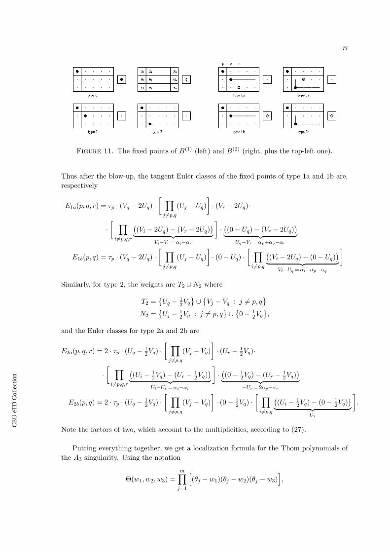
CE
UeT
DC
olle
ctio
n
77
Figure 11. The fixed points of B(1) (left) and B(2) (right, plus the top-left one).
Thus after the blow-up, the tangent Euler classes of the fixed points of type 1a and 1b are,respectively
E1a(p, q, r) = τp · (Vq − 2Uq) ·[ ∏j 6=p,q
(Uj − Uq)]· (Vr − 2Uq)·
·[ ∏i6=p,q,r
((Vi − 2Uq)− (Vr − 2Uq)
)︸ ︷︷ ︸Vi−Vr =αi−αr
]·((0− Uq)− (Vr − 2Uq)
)︸ ︷︷ ︸Uq−Vr =αp+αq−αr
E1b(p, q) = τp · (Vq − 2Uq) ·[ ∏j 6=p,q
(Uj − Uq)]· (0− Uq) ·
[ ∏i6=p,q
((Vi − 2Uq)− (0− Uq)
)︸ ︷︷ ︸Vi−Uq =αi−αp−αq
]
Similarly, for type 2, the weights are T2 ∪N2 where
T2 =Uq − 1
2Vq∪Vj − Vq : j 6= p, q
N2 =
Uj − 1
2Vq : j 6= p, q∪0− 1
2Vq,
and the Euler classes for type 2a and 2b are
E2a(p, q, r) = 2 · τp · (Uq − 12Vq) ·
[ ∏j 6=p,q
(Vj − Vq)]· (Ur − 1
2Vq)·
·[ ∏i6=p,q,r
((Ui − 1
2Vq)− (Ur − 12Vq)
)︸ ︷︷ ︸Ui−Ur =αi−αr
]·((0− 1
2Vq)− (Ur − 12Vq)
)︸ ︷︷ ︸−Ur =2αp−αr
E2b(p, q) = 2 · τp · (Uq − 12Vq) ·
[ ∏j 6=p,q
(Vj − Vq)]· (0− 1
2Vq) ·[ ∏i6=p,q
((Ui − 1
2Vq)− (0− 12Vq)
)︸ ︷︷ ︸Ui
].
Note the factors of two, which account to the multiplicities, according to (27).
Putting everything together, we get a localization formula for the Thom polynomials ofthe A3 singularity. Using the notation
Θ(w1, w2, w3) =m∏j=1
[(θj − w1)(θj − w2)(θj − w3)
],

CE
UeT
DC
olle
ctio
n
78
we have, for n ≥ 3,
TpA3(n,m) =
∑p
Θ(αp, 2αp, 3αp)E0(p)
+∑p,q
[Θ(αp, αq, αp + αq)
E1b(p, q)+
Θ(αp, 2αp, αq)E2b(p, q)
]+(28)
+∑p,q,r
[Θ(αp, αq, αr)E1a(p, q, r)
+Θ(αp, αq, αr)E2a(p, q, r)
].
Indeed, implementing (28) as a computer program, and converting the results to Schurpolynomials in the difference alphabet θ − α (otherwise they would be way too large to fitin a page), we get
TpA3(3, 3) = 6s1,1,1 + 5s2,1 + s3
TpA3(3, 4) = 36s1,1,1,1,1,1 + 30s2,1,1,1,1 + 19s2,2,1,1 + 5s2,2,2 + 6s3,1,1,1 + 5s3,2,1 + s3,3
TpA3(3, 5) = 36s3,1,1,1,1,1,1 + 6s3,3,1,1,1 + 216s1,1,1,1,1,1,1,1,1 + 65s2,2,2,1,1,1+
+ 24s2,2,2,2,1 + 5s3,2,2,2 + s3,3,3 + 114s2,2,1,1,1,1,1 + 5s3,3,2,1+
+ 19s3,2,2,1,1 + 180s2,1,1,1,1,1,1,1 + 30s3,2,1,1,1,1
The phenomenon that these polynomials fit into a Thom series can be observed on theseexamples already: The terms of Tp(n,m) appear in Tp(n,m + 1), but with a 3 preprendedto the partition. Unfortunately, the RHS of (28) is in a form which makes it rather hard toevaluate for larger n,m-s.
Remark. Compare the formula (28) above with Section 3.1, in particular with equations(4) and (6) there. The observation is that by computing the Euler classes at the fixpointsof a B(2), which has a birational dominant map sol : B(2) → M3 ⊂ Hilb3(J3(n)), we canderive the same data for M3 itself, which was not clear how to do directly! We only have torearrange our Euler classes to the form (6), so that a term of the localization formula lookslike
Θ(w1, w2, w3)P (αK) ·
∏i/∈K
[(αi − w1)(αi − w2)(αi − w3)
]where K = i1, . . . , ik ∈
(nk
), and w1, w2, w3 resp. P are linear resp. rational in αK =
αi1 , . . . , αik. In our case, K will be either p, p, q or p, q, r, and the P -s can bereadily read off from the Euler classes; we summarized them in Table 5.
name kQ ideal the rational function P
type 0 1 (x4) P0(p) = 1type 1a 3 (x2, y2, z2, xy, xz, yz) P1a(p, q, r) = (αp − αq)2(αr + αp − 2αq)·
·(αq + αp − αr)(αr − αp)(αq − αr)type 1b 2 (x2, y2) P1b(p, q) = (αp − αq)2(αq − 2αp)type 2a 3 (x2, y2, z2, xy, xz, yz) P2a(p, q, r) = 1
2(αp − αq)2(αq + αp − 2αr)··(2αp − αr)(αr − αp)(αq − αr)
type 2b 2 (x3, xy, y2) P2b(p, q) = 12(αp − αq)2(3αp − αq)
Table 5. Table of fixed points for A3 from the viewpoint of Section 3.1.
To fully convert to the form used in Chapter 3 and [FR08], we have to combine thedifferent fixed points with the same ideal; note that this also includes permutations of the

CE
UeT
DC
olle
ctio
n
79
parameters p, q, r when the ideal has some symmetry! Therefore the final data (comparewith the table in [FR08], Section 8) can obtained as follows:
P(x4) = P0 = 1
P(x2,y2) =[P1b(1, 2)−1 + P1b(2, 1)−1
]−1=
(α1 − α2)2(2α1 − α2)(α1 − 2α2)α1 + α2
P(x3,xy,y2) = P2b(1, 2) = 12(α1 − α2)2(3α1 − α2)
P(x2,y2,z2,xy,xz,yz) =
∑(i,j,k)∈S3
(P1a(i, j, k)−1 + P2a(i, j, k)−1
)−1
= . . .
For reference (it’s omitted from [FR08]), the last expression equals to
· · · = 46(α3
1 + α32 + α3
3)− 7(α21α2 + α2
1α3 + α22α1 + α2
2α3 + α23α1 + α2
3α2) + 10α1α2α3
(α1 − α2 − α3)(α2 − α1 − α3)(α3 − α1 − α2)∏i6=j∈1,2,3(αi − 2αj)
.
We could now in principle apply the ideas of Sections 3.3 and 3.4 to compute the Thomseries of the A3 singularity (which is known by the way, see [BFR02] and [LP09]; how-ever, the methods used in those work are not very elegant and have no chance to scale);unfortunately the actual calculations present rather profound challenges, which are yet toovercome.

CE
UeT
DC
olle
ctio
n
Appendix
The aim of the Appendix is to collect together results, sometimes with proofs, which areused in the main body of the thesis, but would break the flow if presented there.
A.1. Multivariate differentials
Porteous’ probe model for the Thom-Boardman singularities (see Chapter 4, Section4.3.1) deals with higher order differentials of composite functions in many variables; in par-ticular, differentials of the form
d(d(d(F α) β) γ)|0.
Since differential calculus is usually not covered in this generality in university classes andtextbooks, we present a simple graphical calculus to deal with such expressions.
For α ∈ J (n,m), the first differential at x ∈ Cn is (dα)(x) ∈ Hom(TxCn, Tα(x)Cm) =Hom(Cn,Cm). Thus
dα ∈ J(Cn, Hom(Cn,Cm)
)d2α ∈ J
(Cn, Hom(Cn,Hom(Cn,Cm))
)d3α ∈ J
(Cn, Hom(Cn,Hom(Cn,Hom(Cn,Cm)))
)and so on; but of course Hom(Cn,Hom(Cn,Cm)) = Hom(Cn ⊗ Cn,Cm), and we also knowfrom Young’s Theorem that d2α is actually symmetric: d2α : Cn → Hom(Sym2Cn,Cm). Ingeneral
dkα ∈ J(Cn, Hom(SymkCn,Cm)
).
Since we work with both (multi)linear maps and smooth maps between vector spaces,in order to not mix them up, we adopt the (temporary) convention that denotes thecomposition of arbitrary maps, while ∗ denotes the composition of linear maps.
Proposition A.1.1 (Chain rule).(d(α β γ · · · ζ)
)[x] = (dα)
[(β γ · · · ζ)(x)
]∗ (dβ)
[(γ · · · ζ)(x)
]∗ · · · ∗ (dζ)[x].
The next ingredient is the product rule; however, we will need to apply it to varioustensor contractions, so it’s time to introduce a graphical notation. Tensor contractions willbe represented by trees drawn vertically: The nodes correspond to the tensors, the edges tothe contractions, and composition “flows downwards”. For example, the pictures on Figure12 represent the two tensors (written in redundant Einstein notation)
Sijk =∑a,b
(F1)ak(α2)iba (β1)jb
and T ijk =∑a,b,c
(F2)abk (α1)ia(α1)cb(β1)jc,
respectively. These are actually the two terms of the expression d(d(F α) β)|0.80

CE
UeT
DC
olle
ctio
n
81
Figure 12. Examples of our graphical tensor notation.
Proposition A.1.2 (The product rule). Suppose we have such a tensor expression, repre-sented by a tree, as a smooth function of a parameter x ∈ V . Then its differential wrt. x isa sum over the nodes of the tree, and the term corresponding to a fixed node can be drawnby replacing the node with its differential, and attaching a new ‘input leg’, labelled with V ,to symbolize the dependence of this differential on TxV ∼= V .
We can incorporate more complex dependencies on the parameter space by drawing hor-izontal arrows, representing composition of functions. For an example, consider the pictureon the left in Figure 13; this represents the expression
T [x]ijk =∑a,b
(dF )[α(β(x))]ak · (d2α)[β(x)]iba · (dβ)[x]jb.
Putting together the chain rule and the product rule, we get
Proposition A.1.3 (Pictorial rule of tensor differentials). The differential of an expressionof the form shown on Figure 13 is a sum over the (boxed) nodes of the tree, where the termcorresponding to a fixed node can be obtained by replacing that node with its differential,attaching a new leg to it, and attaching to that leg the string of differentials of the incominghorizontal thread (representing the dependence on the parameter space), in accordance withthe chain rule A.1.1.
Figure 13. A more complex example (left), and one of the 3 terms appearingin its derivative (right).

CE
UeT
DC
olle
ctio
n
82
As an example, the picture on the right in Figure 13 is the term corresponding to thenode dF in the differential of the picture on the left.
Corollary A.1.4. The terms of the kth equation in Porteous’ model are in bijection withthe rooted trees with k leaves such that the set of the depths of the leaves is 2, 3, . . . , k+ 1,where the depth is measured as the number of edges from to root the leaf.
Proof. What we need to show is that the terms in the derivatives of the trees with k leavesare exactly the trees with k+1 leaves. But the derivative process, as described above, simplyattaches a “long” thread (with the leaf having depth k + 1) to each existing node in turn.Conversely, starting with a tree with k + 1 leaves, removing the thread of the “deepest”node (with depth k+1) gives back the k-tree and the node (the attach point of the removedthread) whose derivative this tree is.
For an illustration, see Figure 9 on page 69, which shows the k = 3 case (also Figure 12above shows the k = 2 case). The number of such terms (or trees) is growing fast; for k ≤ 8,the counts are
1, 2, 7, 39, 321, 3686, 56516, 1118159, . . .
A.2. Formulae for symmetric polynomials
In this section we collect together various useful formulae for symmetric polynomials,mostly involving Schur polynomials. The canonical reference is [Mac98].
Definition A.2.1. The Schur polynomial indexed by the partition λ = (λ1, . . . , λn) is asymmetric polynomial in the variables x1, . . . , xn defined as the following quotient of twoalternating polynomials:
sλ(x1, . . . , xn) =det[xλj+n−j
i ]n×ndet[xn−ji ]n×n
(29)
Note that the denominator is a Vandermonde determinant (up to sign).
Remark A.2.2. The Schur polynomials can be defined for arbitrary sequences of integers,not just partitions, with the same formulae; and it is true that such a “generalised” Schurpolynomial is either zero or equals to a “usual” Schur polynomial up to sign. Specifically,applying the following transformation finitely many times, we can always obtain a partition(or zero):
s(...,a,b,... ) =−s(...,b−1,a+1... ) a < b− 10 a = b− 1
In formula (29), this corresponds to exchanging columns of the matrix in the numerator, orhaving two identical columns, respectively.
The Jacobi-Trudi formulae express the Schur polynomials in terms of elementary (resp. com-plete) symmetric polynomials:
sλ(x) = det[cµi+j−i(x)] = det[sλi+j−i(x)]
where µ = λ is the dual partition.

CE
UeT
DC
olle
ctio
n
83
Let us introduce two variations of Schur polynomials, which also depend on a secondalphabet y = (y1, . . . , ym). Define ck(x− y) via the equation∏
i(1 + xit)∏j(1 + yjt)
=∞∑k=0
ck(x− y)tk,
where t is a formal variable. Then the supersymmetric Schur polynomials (or Schur polyno-mials in the ‘difference alphabet’) can be defined via the Jacobi-Trudi formula as
sλ(x− y) = det[cµi+j−i(x− y)
]`(µ)×`(µ)
,(30)
where µ = λ is the dual partition. sλ(x − y) is a symmetric polynomial in both set ofvariables.
The double Schur polynomials (or factorial Schur polynomials) sλ(x|y), defined as
(xi|y)k = (xi + y1)(xi + y2) · · · (xi + yk) =k∏j=1
(xi + yj)
sλ(x|y) =det[(xi|y)λj+n−j
]n×n
det[(xi|y)n−j
]n×n
=det[(xi|y)λj+n−j
]n×n
det[xn−ji
]n×n
,(31)
are, in general, symmetric only in the xi variables. For this definition to make sense, we haveeither to assume that m > n+ λ1; or define y>m to be zero.
The two constructions are related by the surprising fact that sλ(x − y) = sλ(x|y∨) inthe limit n → ∞ (see [Mac92]); also both specialize to the usual Schur polynomials whensubstituting y = 0.
In the following, instead of explicit variables x1, . . . , xn, we will work with the Grothendieckring of representations (or even more generally, equivariant vector bundles); for non-virtualrepresentations, the variables are the roots of the representation, but in general they do notexist.
A family of natural questions ask for expressing the Schur polynomials of various derivedrepresentations, eg. symmetric and antisymmetric tensor powers, in terms of the Schurpolynomials of the original representation(s). A compact way to ask these questions is tofind some kind of formula for the coefficients gν1,...,νk
λ;µ1,...,µk∈ Z in the equation
sλ[Sµ1(X1)⊗ Sµ2(X2)⊗ · · · ⊗ Sµk(Xk)
]=∑ν1
∑ν2
· · ·∑νk
gν1,...,νkλ;µ1,...,µk
sν1(X1)sν2(X2) · · · sνk(Xk)
where λ, µi, νi are partitions, and Sµ is the Schur functor corresponding to the partition µ.This is very far from being solved2, however, a few special and very useful cases are known.
Lemma A.2.3 (Pieri’s rule).
sµ(X) · sk(X) =∑λ∈K
sλ(X)
where λ runs over the partitions K which are obtained from µ by adding k boxes to the Youngdiagram of µ, but no two boxes in the same column.
2For example, as we prove in this thesis, these coefficients for k = 1, µ1 = (2) coincide with the coefficients
of the Thom polynomials of Σii singularities, expressed in Schur polynomials.
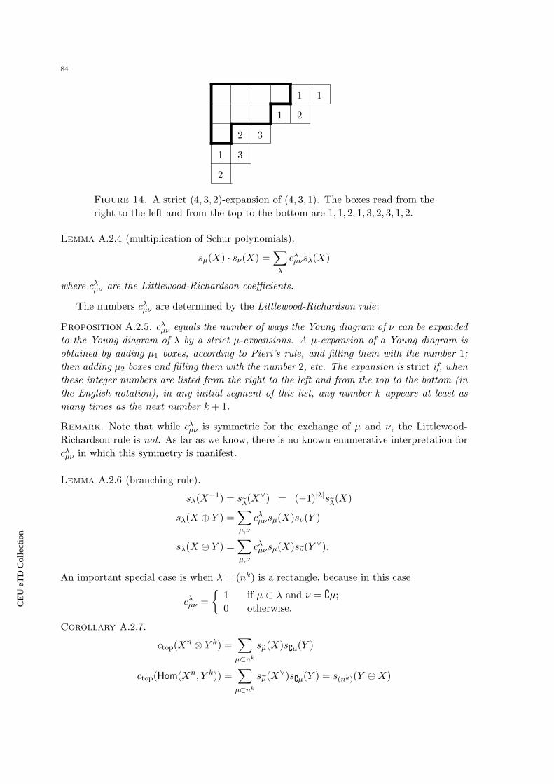
CE
UeT
DC
olle
ctio
n
84
2
1 3
2 3
1 2
1 1
Figure 14. A strict (4, 3, 2)-expansion of (4, 3, 1). The boxes read from theright to the left and from the top to the bottom are 1, 1, 2, 1, 3, 2, 3, 1, 2.
Lemma A.2.4 (multiplication of Schur polynomials).
sµ(X) · sν(X) =∑λ
cλµνsλ(X)
where cλµν are the Littlewood-Richardson coefficients.
The numbers cλµν are determined by the Littlewood-Richardson rule:
Proposition A.2.5. cλµν equals the number of ways the Young diagram of ν can be expandedto the Young diagram of λ by a strict µ-expansions. A µ-expansion of a Young diagram isobtained by adding µ1 boxes, according to Pieri’s rule, and filling them with the number 1;then adding µ2 boxes and filling them with the number 2, etc. The expansion is strict if, whenthese integer numbers are listed from the right to the left and from the top to the bottom (inthe English notation), in any initial segment of this list, any number k appears at least asmany times as the next number k + 1.
Remark. Note that while cλµν is symmetric for the exchange of µ and ν, the Littlewood-Richardson rule is not. As far as we know, there is no known enumerative interpretation forcλµν in which this symmetry is manifest.
Lemma A.2.6 (branching rule).
sλ(X−1) = seλ(X∨) = (−1)|λ|seλ(X)
sλ(X ⊕ Y ) =∑µ,ν
cλµνsµ(X)sν(Y )
sλ(X Y ) =∑µ,ν
cλµνsµ(X)seν(Y ∨).
An important special case is when λ = (nk) is a rectangle, because in this case
cλµν =
1 if µ ⊂ λ and ν = µ;0 otherwise.
Corollary A.2.7.
ctop(Xn ⊗ Y k) =∑µ⊂nk
seµ(X)sµ(Y )
ctop(Hom(Xn, Y k)) =∑µ⊂nk
seµ(X∨)sµ(Y ) = s(nk)(Y X)

CE
UeT
DC
olle
ctio
n
85
Let us introduce the determinant (see Chapter 4, Section 4.5)
Eλ/µ(n) = det
[(λi + n− iµj + n− j
)]n×n
.
Lemma A.2.8 ([Las78]). Let L be a 1 dimensional (virtual) representation. Then
sλ(Xn ⊗ L) =∑µ⊂λ
Eλ/µ(n)sµ(X)s|λ/µ|(L)
c(Xn ⊗ Y k) =∑
µ⊂λ⊂nk
Eλ/µ(k)sµ(Y )seλ(X)
c(∧2Xn) =∑
µ⊂bn−1e
2|µ|−n(n−1)/2 · Ebn−1e/µ(n) · sµ(X)
c(Sym2Xn) =∑µ⊂bne
2|µ|−n(n−1)/2 · Ebne/µ(n) · sµ(X)
where c denotes the total Chern class: c(X) =∑ci(X), and bne = (n, n− 1, n− 2, . . . , 1) is
the ‘stairway’ partition.
A.3. Localization of equivariant cohomology classes
Localization in equivariant cohomology has a rich history, dating back to Duistermaatand Heckman [DH82], Atiyah and Bott [AB84] and Berline and Vergne [BV82, BV83].
We build our treatment on the algebraic theory developed by Edidin and Graham in[EG98a, EG98b], so that the singular case fits into the theory naturally. We can then passto the cohomology version via the so called cycle map. Regarding the intersection theorybackground, we refer to the standard source [Ful98]. We will constrain ourselves to torusactions, which causes no problems in our context, since the GLn-equivariant cohomology isa subring of the Tn-equivariant cohomology for a maximal torus Tn ⊂ GLn.
Lemma A.3.1 ([Ive72]). Let Y be smooth variety with a torus action. Then the fixed pointset Y T is also smooth.
Theorem A.3.2 ([EG98b], Proposition 6). Let f : X → Y be a T-equivariant embeddingof X into a nonsingular variety Y . Assume that every component of Y T which intersects Xis contained in X. For a component F ⊂ XT write iF : F → X and jF = f iF : F → Y
for the corresponding embeddings. Let R = A∗T(pt) ∼= Q[t1, . . . , tn] and Q = (R+)−1R, whereR+ ⊂ R is the multiplicative system of homogeneous elements of positive degree. Then
• f∗ : AT∗ (X)⊗R Q → AT
∗ (Y )⊗R Q is injective;• Let α ∈ AT
∗ (X)⊗R Q. Then
α =∑F⊂XT
(iF )∗j∗F f∗α
ctop(NFY ),
where F runs over the components of XT, and ctop(NFY ) is the T-equivariant top Chernclass (in the Chow ring of F ) of the normal bundle of F in Y .
Remark. Implicit in the theorem is the fact that ctop(NFY ) is invertible in AT∗ (F )⊗Q, see
[EG98b], Proposition 4.

CE
UeT
DC
olle
ctio
n
86
For smooth varieties, we can use the cycle map to pass to the cohomology: For a smoothn-dimensional variety X, we have
ATn−k(X) = AkT(X) cl−−→ H2k
T (X).
See [Ful98], Chapter 19 and [EG98a], sections 2.6, 2.8.
Equivariant localization can be used to compute the pushforward:
Corollary A.3.3. Let π : M → pt be the map collapsing a smooth compact variety M to apoint, and α ∈ H∗
T(M) a cohomology class (it could be a Chow class, too). Assume that Mhas isolated fixed points. Then
π∗α =∑p∈MT
i∗pα
e(TpM)
It can also be used to compute classes of subvarieties.
Corollary A.3.4. In the situation of Theorem A.3.2, we have
[X ⊂ Y ] =∑F⊂XT
(jF )∗j∗F [X ⊂ Y ]e(NFY )
Proof. Use the theorem with α = [X]⊗1 ∈ ATn(X)⊗Q and apply f∗ to the resulting formula.
Note that f∗[X] = [X ⊂ Y ] ∈ ATn(Y ). Finally use the cycle map to pass to the cohomological
version.
Lemma A.3.5. j∗F [X ⊂ Y ] = [NFX ⊂ NFY ] where NFX is the bundle of normal cones ofX along F , embedded into the normal bundle of F in Y .
A direct consequence of the Lemma and the Corollary is the following
Theorem A.3.6 (Localization of classes of subvarieties).
[X ⊂ Y ] =∑F⊂XT
(jF )∗[NFX ⊂ NFY ]
e(NFY )
Topological sketch of proof of Lemma A.3.5. Consider a sequence of “smaller and smaller”tubular neighbourhoods of F in Y :
Y ⊃ N1 ⊃ N2 ⊃ · · · ⊃ Nk ⊃ · · · ⊃ F
with inclusion maps ik : Nk → Y and jk : F → Nk. By the excision property of cohomology,we have
j∗F [X ⊂ Y ] = j∗ki∗k[X ⊂ Y ] = j∗k [(X ∩Nk) ⊂ Nk],
but the latter is “closer and closer” to [NFX ⊂ NFY ].
Algebraic sketch of proof of Lemma A.3.5. Apply the ‘deformation to the normal cone’ con-struction ([Ful98], Chapter 5) to F ⊂ X: Let
X = BlF×∞(X × P1) ⊂ Y = BlF×∞(Y × P1);
the pair (X ,Y)→ P1 is now a (flat) family of embeddings: a deformation from F ⊂ X ⊂ Yat 0 ∈ P1 to F ⊂ NFX ⊂ NFY at ∞ ∈ P1. Apply the ‘principle of continuity’ for flatfamilies.

CE
UeT
DC
olle
ctio
n
87
Our main tool will be the following, less well-known but very useful variation of theabove.
Theorem A.3.7 ([BSz06], [Ros89]). Let V be a representation of a torus T, M be a smoothcompact variety equipped with an action of the torus T, with isolated fixed points, and X ⊂Mbe a (possibly singular) T-invariant closed subvariety. Consider the classifying map ϕ :M →Grr(V ) of a rank r equivariant vector bundle pr1 :E ⊂ M × V → M , and let Y → X thepullback (restriction) of E to X Suppose that ϕ|X : X → ϕ(X) is birational; then Z = pr2(Y )is a closed invariant subvariety of V of dimension dim(Z) = r + dim(X), and
[Z ⊂ V ]T =∑p∈XT
[Yp ⊂ V ]T ·[NpX ⊂ TpM ]T
eT(TpM)∈ H∗
T(pt) = H∗T(V ),
where Yp = pr−11 (p) ⊂ V ×p ∼= V is the fiber over the point p ∈ X, and NpX is the tangent
cone of X at p (the normal cone of X “along” p).
Remark. The quotient e(TpM)[NpX⊂TpM ] is simply e(TpX) if X is smooth at p, and can be thought
as the generalization of the tangent Euler class for singular points. Its inverse is sometimescalled equivariant multiplicity ([Ros89], [Bri97]). Note that it is actually independent ofthe embedding, since the normal cone NpX embeds into the Zariski tangent space TpX whichfurther embeds into TpM ; thus
e(TpM)[NpX ⊂ TpM ]
=e(TpX) · e(TpM/TpX)
[NpX ⊂ TpX] · [TpX ⊂ TpM ]=
e(TpX)[NpX ⊂ TpX]
.
Lemma A.3.8. Let a cyclic group Zk act (diagonally and faithfully) on a torus representationCn. Then for the cyclic quotient singularity X = Cn/Zk, the virtual Euler class is just ktimes the Euler class of Cn (that is, k times the product of weights).
Proof. Direct application of [Bri97], 4.3.
Proof of Theorem A.3.7. First we apply Theorem A.3.6 to the embedding (∆ K) : Y ⊂M×V . Note that since M , and thus X has isolated fixed points, we can classify the fixedcomponents of Y by recording which fixed point p of X they lie over. The following diagramsummarises the situation and the notations:
FjF−−−→ Yp
Ip−−→ YK−−→ E
∆−−−→M × V pr2−−−→ V
πFyπp
yπ yπ pr1
pip−−→ X
k−−→ M
Now
[Z] = (pr2)∗[Y ⊂M×V ] = (pr2)∗∑F⊂Y T
(∆ K Ip jF )∗[NFY ⊂ NF (M×V )]
e(NF (M×V ))=
= (pr2)∗∑p∈XT
(∆ K Ip)∗∑F⊂Y T
p
(jF )∗
([NFYp ⊂ NFVp]
e(NFVp)· (πF )∗
[NpX ⊂ TpM ]e(TpM)
)since NFY is just the product NpX×NFYp (note that F ⊂ Yp is smooth by Lemma A.3.1),and the class of a product is the product of the classes. Now, observe that all our mapsrespect the local product structure around p:
Ip=ip ⊗ id ∆ =id⊗∆p
K=k ⊗ id pr2= pt⊗ id
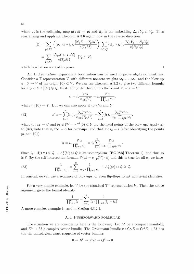
CE
UeT
DC
olle
ctio
n
88
where pt is the collapsing map pt :M → pt and ∆p is the embedding ∆p : Yp ⊂ Vp. Thusrearranging and applying Theorem A.3.6 again, now in the reverse direction:
[Z] =∑p∈XT
((pt k ip)∗
[NpX ⊂ TpM ]e(TpM)
) ∑F⊂Y T
p
(∆p jF )∗[NFYp ⊂ NFVp]
e(NFVp)
=∑p∈XT
[NpX ⊂ TpM ]e(TpM)
· [Yp ⊂ V ],
which is what we wanted to prove.
A.3.1. Application. Equivariant localization can be used to prove algebraic identities.Consider a T-representation V with different nonzero weights w1, . . . , wn, and the blow-upπ : U → V of the origin 0 ⊂ V . We can use Theorem A.3.2 to give two different formulafor any α ∈ AT
k (V )⊗Q. First, apply the theorem to the α and X = Y = V :
α = i∗i∗α
ctop(V )= i∗
i∗α∏nj=1wj
,
where i : 0 → V . But we can also apply it to π∗α and U :
π∗α =n∑k=1
(ik)∗(ik)∗π∗αctop(Tpk
U)=
n∑k=1
(ik)∗(ik)∗π∗α
wk ·∏j 6=k wi
,(32)
where ik : pk → U and pk ∈ PV = π−1(0) ⊂ U are the fixed points of the blow-up. Apply π∗to (32), note that π∗π∗α = α for blow-ups, and that π ik = i (after identifying the pointspk and 0):
α = i∗i∗α∏nj=1wj
= i∗
n∑k=1
i∗α
wk ·∏j 6=k wi
.
Since i∗ : AT∗ (pt) ⊗Q → AT
∗ (V ) ⊗Q is an isomorphism ([EG98b] Theorem 1), and thus sois i∗ (by the self-intersection formula i∗i∗β = ctop(V ) · β) and this is true for all α, we have
1∏nj=1wj
=n∑k=1
1wk ·
∏j 6=k wi
∈ A∗T(pt)⊗Q ∼= Q.(33)
In general, we can use a sequence of blow-ups, or even flip-flops to get nontrivial identities.
For a very simple example, let V be the standard Tn-representation V . Then the aboveargument gives the formal identity
1∏nj=1 ti
=n∑k=1
1tk ·∏j 6=k(tj − tk)
.
A more complex example is used in Section 4.3.2.1.
A.4. Pushforward formulae
The situation we are considering here is the following. Let M be a compact manifold,and En →M a complex vector bundle. The Grassmann bundle π : GrrE = GrqE →M hasthe the tautological exact sequence of vector bundles
0→ Rr → π∗E → Qq → 0

CE
UeT
DC
olle
ctio
n
89
over it. We are interested in formulae expressing the pushforward map
π∗ : H∗(GrqE)→ H∗−2rq(M).
There are variations of this theme for partial flag bundles, sequences of vector bundles, etc.
Theorem A.4.1. Assuming the situation described above, and that `(λ) ≤ q, `(µ) ≤ r, wehave
π∗sλ(Q) = s(λ−rq)(E);(34)
π∗sµ(R) = (−1)rqs(µ−qr)(E);(35)
π∗[sµ(R)sλ(Q)] = s(λ−rq ,µ)(E).(36)
Furthermore, if F →M is another vector bundle,
π∗[sµ(R|F )sλ(Q|F )] = s(λ−rq ,µ)(E|F );(37)
π∗[sµ(R− F )sλ(Q− F )] = s(λ−rq ,µ)(E − F ).(38)
The same formulae are true for the universal bundle, and equivariant vector bundles too;and also for Chow groups instead of cohomology.
Remarks. Both (34) and (35) are special cases of (36), which itself is special case of both(37) and (38). The RHS of these formulae should be understood according to Remark A.2.2,which explains the sign in (35). The most useful variation (38) is proved in [JLP82, Pra88].The case (35) was also proved in [Ron72]. As far as we now, (37) is new.
In the remaining part of the section, we give a simple geometric proof of (37), usingequivariant localization. We believe this proof can be adapted to the last case (38) too, forexample using the so-called Sergeev-Pragacz formula for the supersymmetric Schur polyno-mials.
A geometric representation. For the proof, we will need a geometric representationfor the Schur classes sλ(E); consider the following construction. Let En be the standardGLn representation; fix a large integer N 0, the standard representation FN of GLN , anda complete flag K• in F∨:
0 = K0 < K1 < K2 < · · · < KN = F∨, dim(Kj) = j.
Denote by BN the Borel subgroup of GLN fixing K•. Let τ be a partition
N ≥ τ1 ≥ τ2 ≥ · · · ≥ τn ≥ 0.
Consider Flτ (E∨), the variety of partial flags in the dual space E∨ with dimensions corre-sponding to τj : j: points of Flτ (E∨) correspond to sequences A• of linear subspaces
0 < · · · < Ai < · · · ≤ E∨, dim(Ai) = i, (i, ∗) ∈ corner(τ).
Here corner denotes the set of outer corners of the Young diagram of a partition:
corner(µ) =
(i, j) ∈ N× N : µi = j, µj = i.
If τ is a strict partition, Flτ is simply the complete flag variety. Let ek denote the (ordered)set of the dimensions of the subspaces in A•:
e1, e2, . . . , el
=i : (i, ∗) ∈ corner(τ)
, l = |corner(τ)|,

CE
UeT
DC
olle
ctio
n
90
(note that 0 < ek ≤ n; for convenience, set e0 = 0), and let dτ denote the dimension of Flτ :
dτ = dim(Flτ (E∨)) =l∑
k=1
(ek − ek−1)(n− ek) ≤(n
2
).
Now consider the vector bundle pr1 : Sτ → Flτ (E∨) of subspaces of E ⊗F , where elements ofE ⊗ F are thought as bilinear functions on E∨ × F∨:
Sτ =
(A•, f) ∈ Flτ (E∨)× E ⊗ F : f |Ai⊗Kj = 0, (i, j) ∈ corner(τ)
and let Sτ = pr2(Sτ ) be the image of Sτ in E ⊗ F .
Lemma A.4.2. Sτ is a GLn × BN -invariant closed subvariety of E ⊗ F of codimension
codim(Sτ ) = |τ | − dτ ≥ |τ | −(n
2
),
with equality if and only if τ is a strict partition.
Proof. The only thing not clear here is the (co)dimension. However, Sτ → Flτ is GLn-equivariant by construction, and it is easy to see that for any flag A• the stabiliser of thefibrum XA• = pr−1
1 (A•) is the same as the stabiliser of pr2(XA•), from which the codimensionformula follows using the simple fact that codim(XA•) = |τ |.
Remark. The unique flag A• ∈ Flτ corresponding to a generic map f ∈ Sτ isAi = coker(f †|Kj ) : (i, j) ∈ corner(τ)
where f † is the image of f at the canonical isomorphism E⊗F → Hom(F∨, E). Alternatively,it can be also found algorithmically, by applying the Gaussian elimination process to thematrix of f , where on F we choose a basis compatible with K•.
If τ is a strict partition, let us denote by λ the partition λ = τ − bn− 1e (that is,λi = τi−n+ i), and use the alternative name Zλ for Sτ . In this case Flτ is the complete flagvariety, codim(Zλ) = |λ|, and
Lemma A.4.3. Zλ represents the classes
[Zλ]GLn×BN= sλ(E|F ) ∈ H∗
GLn×BN(E ⊗ F ).
Proof. The proof is a direct application of Theorem A.3.7. As always, we can reduce GLn×BNto its maximal torus Tn × TN . The fixed points of the complete flag variety Fl(E∨) are thecoordinate flags, indexed by permutations of n. Let
x1, . . . , xn and y1, . . . , yN
denote the weights of E and F , respectively; then the weights of the tangent space representa-tion TσFl(E∨) at the fixed flag corresponding to the permutation σ ∈ Sn are −xσ(j)+xσ(i) :j > i , thus the equivariant Euler class eT(TσFl(E∨)) is
eT(TσFl(E∨)
)= sgn(σ)
∏j>i
(xi − xj) = det[xn−ji
].
Choosing a basis of F∨ such that theKj are coordinate subspaces, the fiber Zσ ⊂ Hom(E∨, F )over σ ∈ Sn consists of the matrices of the form
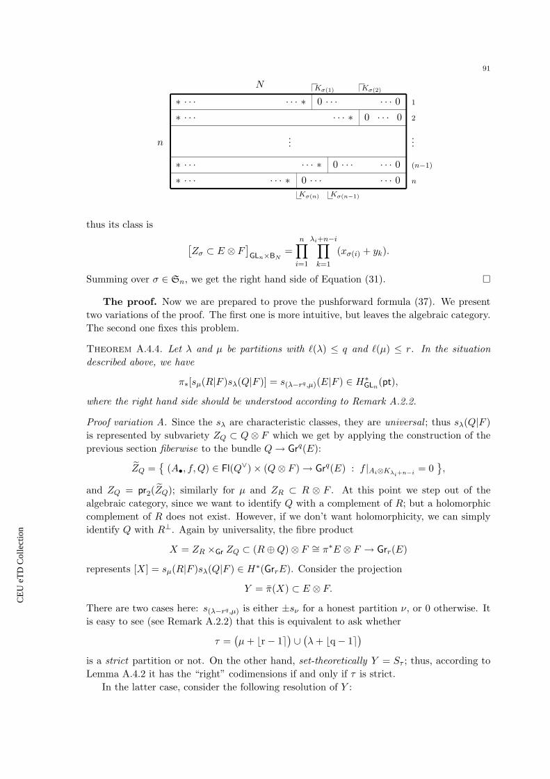
CE
UeT
DC
olle
ctio
n
91
...n
N
n
(n−1)
...
2
1
Kσ(n) Kσ(n−1)
Kσ(2)Kσ(1)
∗ · · ·∗ · · ·
∗ · · ·∗ · · ·
· · · ∗· · · ∗
· · · ∗· · · ∗
0 · · ·0 · · ·
0 · · · 0
0 · · ·
· · · 0· · · 0
· · · 0
thus its class is [Zσ ⊂ E ⊗ F
]GLn×BN
=n∏i=1
λi+n−i∏k=1
(xσ(i) + yk).
Summing over σ ∈ Sn, we get the right hand side of Equation (31).
The proof. Now we are prepared to prove the pushforward formula (37). We presenttwo variations of the proof. The first one is more intuitive, but leaves the algebraic category.The second one fixes this problem.
Theorem A.4.4. Let λ and µ be partitions with `(λ) ≤ q and `(µ) ≤ r. In the situationdescribed above, we have
π∗[sµ(R|F )sλ(Q|F )] = s(λ−rq ,µ)(E|F ) ∈ H∗GLn
(pt),
where the right hand side should be understood according to Remark A.2.2.
Proof variation A. Since the sλ are characteristic classes, they are universal ; thus sλ(Q|F )is represented by subvariety ZQ ⊂ Q ⊗ F which we get by applying the construction of theprevious section fiberwise to the bundle Q→ Grq(E):
ZQ =
(A•, f,Q) ∈ Fl(Q∨)× (Q⊗ F )→ Grq(E) : f |Ai⊗Kλi+n−i= 0
,
and ZQ = pr2(ZQ); similarly for µ and ZR ⊂ R ⊗ F . At this point we step out of thealgebraic category, since we want to identify Q with a complement of R; but a holomorphiccomplement of R does not exist. However, if we don’t want holomorphicity, we can simplyidentify Q with R⊥. Again by universality, the fibre product
X = ZR ×Gr ZQ ⊂ (R⊕Q)⊗ F ∼= π∗E ⊗ F → Grr(E)
represents [X] = sµ(R|F )sλ(Q|F ) ∈ H∗(GrrE). Consider the projection
Y = π(X) ⊂ E ⊗ F.
There are two cases here: s(λ−rq ,µ) is either ±sν for a honest partition ν, or 0 otherwise. Itis easy to see (see Remark A.2.2) that this is equivalent to ask whether
τ =(µ+ br− 1e
)∪(λ+ bq− 1e
)is a strict partition or not. On the other hand, set-theoretically Y = Sτ ; thus, according toLemma A.4.2 it has the “right” codimensions if and only if τ is strict.
In the latter case, consider the following resolution of Y :

CE
UeT
DC
olle
ctio
n
92
Y =
(U•, fR, fQ) ∈ Flτ (E∨)× (Ur ⊗ F )× (U⊥r ⊗ F )
: f |Ui⊗Kµi+r−i = 0 ∀i ≤ r, g|(Uj∩U⊥r )⊗Kλj−r+q−(j−r)
= 0 ∀j > r.
The following diagram summarises the situation:
Hom(π∗E,F ) π−−→ Hom(E,F )x xY
α−−→ ZR ×Gr ZQπ−−→ Yy y y
Fl(E) α−−→ Grr(E) π−−→ pt
where α(U•) = Ur and α(U•, f, g) = (Ur, f, g). Applying Theorem A.3.7 to Y gives thedesired result, similarly as in the proof of Lemma A.4.3. The sign comes from the differentorder of (µ+ br− 1e)∪ (λ+ bq− 1e) and (µ+ br− 1e, λ+ bq− 1e) (it will be the sign of thepermutation between the two; cf. Remark A.2.2).
Remark. It is in fact not surprising that the above proof does not work in the algebraiccategory: equivariant cohomology classes (also called multidegrees) represented by complexalgebraic varieties are always “positive”, similarly as degrees of projective varieties are pos-itive. By “positive”, we mean that it is in the cone spanned by the weights of the ambientrepresentation, which is E⊗F in our case. However, we have a sign in our formula, depend-ing on the relation of λ and µ, that is, depending on the geometry and not just, say, theconventions. Nonetheless, the proof works in the algebraic category if either µ = 0 or λ = 0,which gives the idea for the second variation below.
Proof variation B. We will calculate the pushforward of
sµ(R∨|F∨)sλ(Q|F ) = (−1)|µ|sµ(R|F )sλ(Q|F ).
For this, consider the varieties
XQ = (q ⊗ id)−1(ZQ ) ⊂ E ⊗ F → Grq(E) and
XR∨ = (i∨ ⊗ id)−1(ZR∨) ⊂ E∨ ⊗ F∨ → Grr(E∨) = Grq(E),
where i and q are the tautological inclusion and factor maps:
Ri−−−→ E
q−−−→ Q ;
R∨i∨←−−− E∨ q∨←−−− Q∨ .
We still have [XQ] = sλ(Q|F ) and [XR∨ ] = sµ(R∨|F∨), and thus[XQ ×XR∨ ⊂ (E ⊗ F )⊕ (E∨ ⊗ F∨)→ Grq(E)
]= sµ(R∨|F∨)sλ(Q|F ).
Note that there is a canonical isomorphism
Fl(Q∨)×GrFl(R) −→ Fl(E∨)A1, . . . , Aq , B1, . . . , Br 7−→
A1, . . . , Aq = (E/Br)∨, . . . , (E/B1)∨, E∨
and we can compute the class π∗[X] = [π(X)] using Theorem A.3.7, as before.

CE
UeT
DC
olle
ctio
n
93
A.5. Basic hypergeometric series
Here we collect the definitions and theorems we use from the theory of basic hypergeo-metric3, or q-hypergeometric series. We refer to [GR90] for the details.
Definition A.5.1 (The q-shifted factorial).
(a; q)∞ =∞∏k=0
(1− aqk)
(a; q)n =(a; q)∞
(aqn; q)∞=
(1− a)(1− aq)(1− aq2) · · · (1− aqn−1) n > 01 n = 01/[(1− aq−1)(1− aq−2) · · · (1− aq−n)
]n < 0
We will sometimes use the shorthand notation
(a1, a2, . . . ak; q)n =k∏i=1
(ai; q)n
Definition A.5.2 (The q-binomial coefficient).[n
k
]q
=(q; q)n
(q; q)k(q; q)n−k
Definition A.5.3 (The basic hypergeometric (or q-hypergeometric, or Heine’s) series).
2Φ1
[a, b
c
∣∣∣ q, z] =∞∑n=0
(a; q)n(b; q)n(q; q)n(c; q)n
zn
Definition A.5.4 (The generalized q-hypergeometric series).
rΦs
[a1, a2, . . . , arb1, . . . , bs
∣∣∣ q, z] =∞∑n=0
(a1, . . . , ar; q)n(q, b1, . . . , bs; q)n
[(−1)nq(
n2)](1+s−r)
zn
One of the fundemental results in the subject is the q-binomial theorem:
Theorem A.5.5. For |z| < 1 and |q| < 1∞∑n=0
(a; q)n(q; q)n
zn =(az; q)∞(z; q)∞
A general trick is letting a parameter tend to infinity. For example:
Corollary A.5.6. Setting z = z/a and letting a→∞ in the q-binomial theorem, we get∞∑n=0
(−1)nq(n2)
(q; q)nzn = (z; q)∞
Theorem A.5.7 (Finite q-binomial theorem).
(ab; q)n =n∑k=0
[n
k
]q
bk(a; q)k(b; q)n−k
The Theorem A.5.5 follows from this one by setting b = z and letting n tend to infinity.
3The word ‘basic’ refers to ‘base q’; for example there are ‘bibasic’ series too, which contain two parameters
p and q.
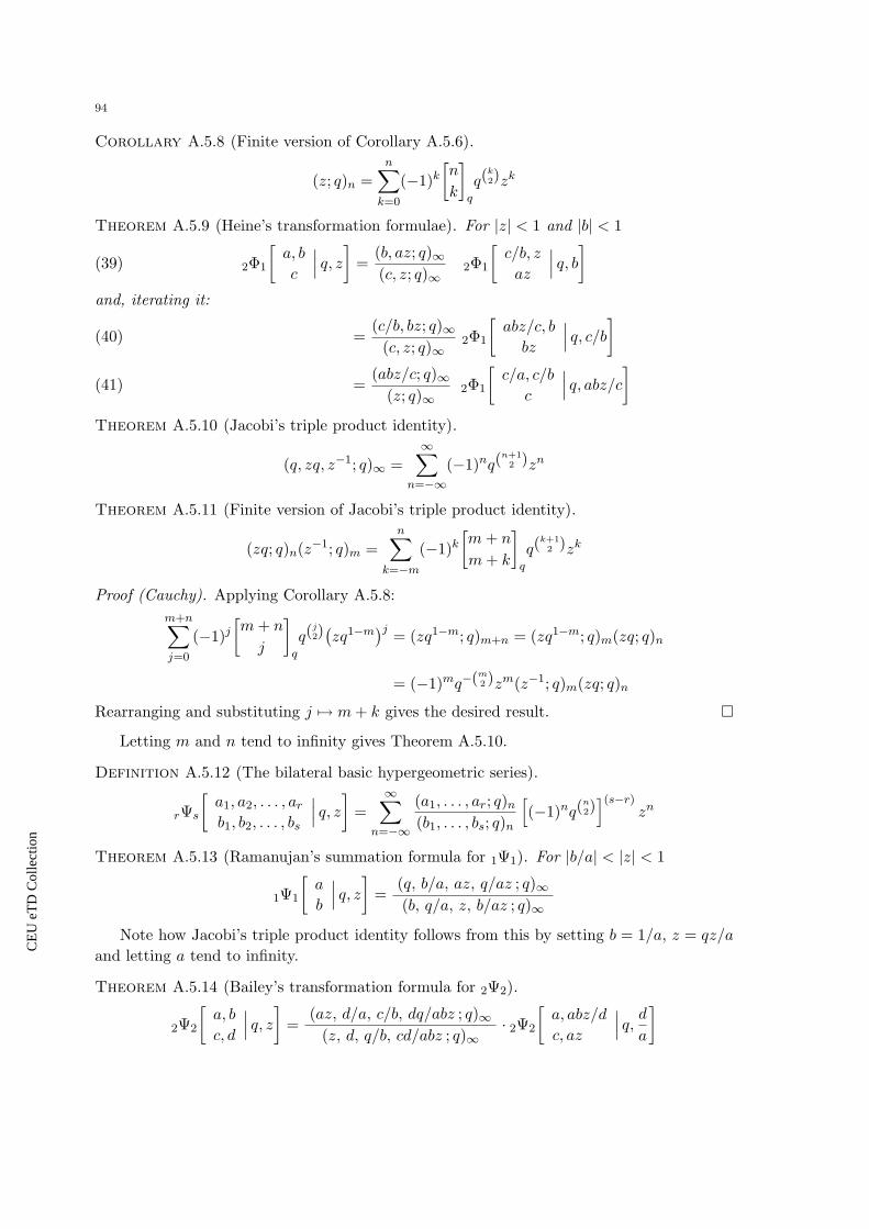
CE
UeT
DC
olle
ctio
n
94
Corollary A.5.8 (Finite version of Corollary A.5.6).
(z; q)n =n∑k=0
(−1)k[n
k
]q
q(k2)zk
Theorem A.5.9 (Heine’s transformation formulae). For |z| < 1 and |b| < 1
2Φ1
[a, b
c
∣∣∣ q, z] =(b, az; q)∞(c, z; q)∞
2Φ1
[c/b, z
az
∣∣∣ q, b](39)
and, iterating it:
=(c/b, bz; q)∞
(c, z; q)∞2Φ1
[abz/c, b
bz
∣∣∣ q, c/b](40)
=(abz/c; q)∞
(z; q)∞2Φ1
[c/a, c/b
c
∣∣∣ q, abz/c](41)
Theorem A.5.10 (Jacobi’s triple product identity).
(q, zq, z−1; q)∞ =∞∑
n=−∞(−1)nq(
n+12 )zn
Theorem A.5.11 (Finite version of Jacobi’s triple product identity).
(zq; q)n(z−1; q)m =n∑
k=−m(−1)k
[m+ n
m+ k
]q
q(k+12 )zk
Proof (Cauchy). Applying Corollary A.5.8:m+n∑j=0
(−1)j[m+ n
j
]q
q(j2)(zq1−m
)j = (zq1−m; q)m+n = (zq1−m; q)m(zq; q)n
= (−1)mq−(m2 )zm(z−1; q)m(zq; q)n
Rearranging and substituting j 7→ m+ k gives the desired result.
Letting m and n tend to infinity gives Theorem A.5.10.
Definition A.5.12 (The bilateral basic hypergeometric series).
rΨs
[a1, a2, . . . , arb1, b2, . . . , bs
∣∣∣ q, z] =∞∑
n=−∞
(a1, . . . , ar; q)n(b1, . . . , bs; q)n
[(−1)nq(
n2)](s−r)
zn
Theorem A.5.13 (Ramanujan’s summation formula for 1Ψ1). For |b/a| < |z| < 1
1Ψ1
[a
b
∣∣∣ q, z] =(q, b/a, az, q/az ; q)∞(b, q/a, z, b/az ; q)∞
Note how Jacobi’s triple product identity follows from this by setting b = 1/a, z = qz/a
and letting a tend to infinity.
Theorem A.5.14 (Bailey’s transformation formula for 2Ψ2).
2Ψ2
[a, b
c, d
∣∣∣ q, z] =(az, d/a, c/b, dq/abz ; q)∞
(z, d, q/b, cd/abz ; q)∞· 2Ψ2
[a, abz/d
c, az
∣∣∣ q, da
]

CE
UeT
DC
olle
ctio
n
Bibliography
[AB84] Michael F. Atiyah and Raoul Bott, The moment map and equivariant cohomology, Topology 23
(1984), no. 1, 1–28.
[AVGL98] V. I. Arnold, V. A. Vasil’ev, V. V. Goryunov, and O. V. Lyashko, Singularity theory I., Springer,
1993, 1998, Originally published as Vol. 6 in the series: Encyclopaedia of Mathematical Sciences.
[BSz06] Gergely Berczi and Andras Szenes, Thom polynomials of Morin singularities, arXiv:math/0608285,
2006.
[Ber08] Gergely Berczi, Multidegrees of singularities and nonreductive quotients, Ph.D. thesis, Budapest
University of Technology, 2008.
[BFR02] Gergely Berczi, Laszlo M. Feher, and Richard Rimanyi, Expressions for resultants coming from the
global theory of singularities, Topics in Algebraic and Noncommutative Geometry (L. McEwan,
J. P. Brasselet, C. Melles, G. Kennedy, and K. Lauter, eds.), Contemporary Mathematics, vol.
324, AMS, 2002.
[Boa67] J. Michael Boardman, Singularities of differentiable maps, Inst. Hautes Etudes Sci. Publ. Math
33 (1967), 21–57.
[Bri97] Michel Brion, Equivariant Chow groups for torus actions, Transformation Groups 2 (1997), no. 3,
225–267.
[BV82] Nicole Berline and Michele Vergne, Classes caracteristiques equivariantes. Formule de localisation
en cohomologie equivariante, C. R. Acad. Sci. Paris Ser. I Math 295 (1982), 539–541.
[BV83] , Zeros d’un champ de vecteurs et classes characteristiques equivariantes, Duke Math. J.
50 (1983), no. 2, 539–549.
[Dam72] James Damon, Thom polynomials for contact class singularities, Ph.D. thesis, Harvard, 1972.
[DH82] J. J. Duistermaat and G. J. Heckman, On the variation in the cohomology of the symplectic form
of the reduced phase space, Invent. Math. 69 (1982), no. 2, 259–268.
[EG98a] Dan Edidin and William Graham, Equivariant intersection theory, Invent. Math. 131 (1998), no. 3,
595–634.
[EG98b] , Localization in equivariant intersection theory and the Bott residue formula, Amer. J.
Math. 120 (1998), no. 3, 619–636.
[Eis95] David Eisenbud, Commutative algebra with a view toward algebraic geometry, GTM, vol. 150,
Springer, 1995.
[FK06] Laszlo M. Feher and Balazs Komuves, On second order Thom-Boardman singularities, Fundamenta
Mathematicae 191 (2006), no. 3, 249–264.
[FNR05] Laszlo M. Feher, Andras Nemethi, and Richard Rimanyi, Degeneracy of 2-forms and 3-forms,
Canad. Math. Bull. 48 (2005), no. 4, 547–560.
[FP98] William Fulton and Piotr Pragacz, Schubert varieties and degeneracy loci, LNM, vol. 1689,
Springer, 1998.
[FR04] Laszlo M. Feher and Richard Rimanyi, Calculation of Thom polynomials and other cohomological
obstructions for group actions, Real and complex singularities, Contemp. Math, vol. 354, AMS,
Providence, R.I., 2004, pp. 69–93.
[FR06] , Thom polynomial computing strategies. A survey, Singularity Theory and Its Applications,
Adv. Studies in Pure Math., vol. 43, Math. Soc. Japan, 2006, pp. 45–53.
[FR07] , On the structure of Thom polynomials of singularities, Bull. London Math. Soc. 39 (2007),
no. 4, 541–549.
[FR08] , Thom series of contact singularities, arXiv:0809.2925, 2008.
[Fra09] Matthias Franz, Convex - a Maple package for convex geometry, published electronically at
http://www.math.uwo.ca/∼mfranz/convex/, 2009.
[Ful96] William Fulton, Schubert varieties in flag bundles for the classical groups, Procs. of the Hirzebruch
65 Conference on Algebraic Geometry, Israel Math. Conf. Proc., vol. 9, 1996, pp. 241–262.
[Ful98] , Intersection theory, Springer-Verlag, 1994, 1998.
[Gaf83] Terence Gaffney, The Thom polynomial ofP1111, Singularities, Part 1 (Arcata, Calif., 1981), Proc.
Sympos. Pure Math, vol. 40, AMS, 1983, pp. 399–408.
[GH78] Phillip Griffiths and Joseph Harris, Principles of algebraic geometry, Wiley-Interscience, 1978.
95
CE
UeT
DC
olle
ctio
n
96
[GHC] The Glasgow Haskell Compilation System, http://haskell.org/ghc/.
[GR90] George Gasper and Mizan Rahman, Basic hypergeometric series, Cambridge Univ. Press, 1990.
[Har95] Joe Harris, Algebraic geometry. A first course, GTM, vol. 133, Springer-Verlag, 1995.
[HK57] A. Haefliger and A. Kosinski, Un theoreme de Thom sur les singularites des applications
differentiables, Seminaire Henri Cartan, vol. 9, 1956–1957, Expose 8.
[HT84] Joe Harris and Loring W. Tu, On symmetric and skew-symmetric determinantal varieties, Topology
23 (1984), no. 1, 71–84.
[Ive72] Birger Iversen, A fixed point formula for action of tori on algebraic varieties, Invent. Math. 16
(1972), 229–236.
[JLP82] Tadeusz Jozefiak, Alain Lascoux, and Piotr Pragacz, Classes of determinantal varieties associated
with symmetric and antisymmetric matrices, Math. USSR Izvestija 18 (1982), 575–586.
[Kaz06] Maxim E. Kazarian, Remark on Thom polynomials for I2,2 and Σa,b, private communication, 2006.
[Las78] Alain Lascoux, Classes de Chern d’un produit tensoriel, C. R. Acad. Sci. Paris, Ser. A 286 (1978),
385–387.
[LP00] Alain Lascoux and Piotr Pragacz, Schur Q-functions and degeneracy locus formulas for morphisms
with symmetries, Recent Progress in Intersection Theory (G. Ellingsrud, W. Fulton, and A. Vistoli,
eds.), Trends in Mathematics, 2000, pp. 239–263.
[LP09] , Thom polynomials and Schur functions: the singularities A3(−), to appear in Publications
of RIMS; http://www.impan.pl/∼pragacz, 2009.
[Mac92] Ian G. Macdonald, Schur functions: Theme and variations, Seminaire Lotharingien de Combina-
toire 28 (1992), 5–39.
[Mac98] , Symmetric functions and Hall polynomials, Oxford University Press, 1979, 1998.
[Mat73] John N. Mather, On Thom-Boardman singularities, Dynamical Systems (Proc. Sympos. Univ.
Bahia, Salvador, 1971), 1973, pp. 233–248.
[OEIS] Neil J. A. Sloane, The On-Line Encyclopedia of Integer Sequences, published electronically at
http://http://www.research.att.com/∼njas/sequences/.
[PJ03] Simon Peyton-Jones, The Haskell 98 language and libraries: The revised report, Journal of Func-
tional Programming 13 (2003), no. 1, http://www.haskell.org.
[Por71] Ian R. Porteous, Simple singularities of maps, Proceedings of Liverpool Singularities Symposium,
I (1969/70), LNM, vol. 192, Springer, 1971, pp. 286–307.
[Por83] , Probing singularities, Singularities, Part 2 (Arcata, Calif., 1981), Proc. Sympos. Pure
Math, vol. 40, AMS, 1983, pp. 395–406.
[Pra88] Piotr Pragacz, Enumerative geometry of degeneracy loci, Ann. Sci. Ecole Norm. Sup. 21 (1988),
no. 3, 413–454.
[Pra90] , Cycles of isotropic subspaces and formulas for symmetric degeneracy loci, Topics in Alge-
bra (S. Balcerzyk et al., ed.), vol. 26, Banach Center Publications, no. 2, 1990, pp. 189–199.
[Pra07] , Thom polynomials and Schur functions: the singularities I2,2(−), Ann. Inst. Fourier 57
(2007), no. 5, 1487–1508.
[PW07a] Piotr Pragacz and Andrzej Weber, Positivity of Schur function expansions of Thom polynomials,
Fundamenta Mathematicae 195 (2007), 85–95.
[PW07b] , Thom polynomials of invariant cones, Schur functions, and positivity, Algebraic cycles,
sheaves, shtukas, and moduli, Trends in Math., 2007, pp. 117–129.
[Rim01] Richard Rimanyi, Thom polynomials, symmetries and incidences of singularities, Inv. Math. 143
(2001), 499–521.
[Ron72] Felice Ronga, Le calcul des classes duales aux singularites de Boardman d’ordre deux, Comment.
Math. Helv. 47 (1972), 15–35.
[Ros89] Wulf Rossmann, Equivariant multiplicities on complex varieties, Orbites unipotentes et
representations, III. Orbites et faisceaux pervers, Asterisque, vol. 173–174, 1989, pp. 313–330.
[Sta99] Richard P. Stanley, Enumerative combinatorics, Cambridge University Press, 1997, 1999.
[Ste05] John R. Stembridge, A Maple package for symmetric functions, published electronically at
http://www.math.lsa.umich.edu/∼jrs/software/SF.ps, 2005.
[Tho56] Rene Thom, Les singularites des applications differentiables, Ann. Inst. Fourier, Grenoble 6 (1956),
43–87.