on bayesian analysis of mixtures with an unknown …mapjg/papers/... · j. r. statist. soc. b...
TRANSCRIPT

J. R. Statist. Soc. B (1997) 59, No. 4, pp. 731-792
On Bayesian Analysis of Mixtures with an Unknown Number of Components
By SYLVIA RICHARDSON and PETER J. GREEN?
Institut National de la Santd et de la Recherche University of Bristol, UK Medicale, Villejuif. France
[Read before The Royal Statistical Society at a meeting organized by the Research Section on Wednesday, January 15th. 1997, the President, Professor A. F . M. Smith, in the Chair]
SUMMARY New methodology for fully Bayesian mixture analysis is developed, making use of reversible jump Markov chain Monte Carlo methods that are capable of jumping between the parameter subspaces corresponding to different numbers of components in the mixture. A sample from the full joint distribution of all unknown variables is thereby generated, and this can be used as a basis for a thorough presentation of many aspects of the posterior distribution. The methodology is applied here to the analysis of univariate normal mixtures, using a hierarchical prior model that offers an approach to dealing with weak prior information while avoiding the mathematical pitfalls of using improper priors in the mixture context.
Keywords: BIRTH-AND-DEATH PROCESS; CLASSIFICATION; GALAXY DATA; HETEROGENEITY; LAKE ACIDITY DATA; MARKOV CHAIN MONTE CARL0 METHOD; NORMAL MIXTURES; PREDICTIVE DISTRIBUTION; REVERSIBLE JUMP ALGORITHMS; SENSITIVITY ANALYSIS
1. INTRODUCTION
This paper is a contribution to the methodology of fully Bayesian mixture modelling. We stress the word 'fully' in two senses. First, we model the number of components and the mixture component parameters jointly and base inference about these quantities on their posterior probabilities. This is in contrast with most previous Bayesian treatments of mixture estimation, which consider models for different numbers of components separately and use significance tests or other non-Bayesian criteria to infer the number of components. Secondly, we aim to present posterior distributions of our objects of inference (model parameters and predictive densities), and not just 'best estimates'.
There are three key ideas in our treatment. First, we demonstrate that novel Markov chain Monte Carlo (MCMC) methods,
the 'reversible jump' samplers introduced by Green (1994, 1995), can be used to sample mixture representations with an unknown and hence varying number of components. We believe that these methods are preferable on grounds of con-venience, accuracy and flexibility to the use of analytic approximations or other recently proposed MCMC techniques.
Secondly, we show that a sample-based approach to computation in mixture models allows a much more subtle extraction of information from posterior distributions. We give examples of presentation from posteriors that tease out
tAddress for correspondence: Department of Mathematics, University of Bristol, University Walk, Bristol, BS8 ITW, UK. E-mail: [email protected]
O 1997 Royal Statistical Society 00359246/97/59731

732 RICHARDSON AND GREEN [No. 4,
alternative explanations of the data, which would be difficult to discover by other approaches.
Finally, we base our experiments and discussion on a hierarchical model for mixtures that aims to provide a simple and generalizable way of being weakly informative about parameters of mixture models. We propose a specific model for univariate normal mixtures, used throughout to illustrate implementation and performance, but emphasize that the rest of our methodology is in no way restricted to this particular model.
Some of the issues considered in the paper, including the key ideas above, have relevance well beyond mixture problems. In particular, issues concerning the presentation of posterior distributions arise in many problems of inference about functions, and the interesting questions raised about labelling of parameters occur whenever the statistical model has partial invariance to permutations of variables.
Since the beginning of the century, there has been strong and sustained interest in finite mixture distributions, attributed to the complementary aspects of mixture models: they provide, first, a natural framework for the modelling of heterogeneity, thereby establishing links with cluster analysis and, secondly, an appealing semi- parametric structure in which to model unknown distributional shapes, whether the objective is density estimation or the flexible construction of Bayesian priors. The whole field is comprehensively discussed by Titterington et al. (1985) and McLachlan and Basford (1988).
Statistical analysis of mixtures has not been straightforward, with non-standard problems posed by the geometry of the parameter space, and also computational difficulties. Headway has been made recently both in dealing with the challenging distributional problems in testing hypotheses about the number of mixture com- ponents (Dacunha-Castelle and Gassiat, 1997; Lindsay, 1995; Feng and McCulloch, 1996) and, on the computational side, by implementation of variants of the EM algorithm (Celeux et al., 1996). However, we strongly believe that the Bayesian paradigm is particularly suited to mixture analysis especially with an unknown number of components.
Much previous work on finite mixture estimation, Bayesian or otherwise, has separated the issues of testing the number of components k from estimation with k fixed. For the fixed k case, a comprehensive Bayesian treatment using MCMC methods has been presented in Diebolt and Robert (1994). Early approaches to the general case where k is unknown typically adopted a different style of modelling, treating the problem as an example of 'Bayesian nonparametrics', and basing prior distributions on the Dirichlet process; see Escobar and West (1995) for example. Other researchers, e.g. Mengersen and Robert (1996), Raftery (1996) and Roeder and Wasserman (1997), have proposed to use respectively a Kullback-Leibler dis-tance, a Laplace-Metropolis estimator or a Schwarz criterion to choose the number of components. The more direct line that we adopt here, of modelling the unknown k case by mixing over the fixed k case, and making fully Bayesian inference, has been followed by only a few researchers, including Nobile (1994) and Phillips and Smith (1 996).
The paper is structured as follows. In Section 2, we present a Bayesian hierarchical model for mixtures. MCMC methods for variable dimension problems are discussed in Section 3, and then adapted to the particular case of mixture analysis. In Section 4, the performance of the methodology is assessed through application to three real

19971 BAYESIAN ANALYSIS OF MIXTURES 733
data sets, and in Sections 5 and 6 sensitivity and MCMC performance issues are considered. Section 7 covers classification based on mixture modelling, and we con- clude with a discussion of extensions and an outline of further work.
2. BAYESIAN MODELS FOR MIXTURES
2.1. Basic Formulation We write the basic mixture model for independent scalar or vector observations yi
as
Yi --xk wj f(.lej) independently for i = 1, 2, . . ., n, (1) j=I
where f(.l8) is a given parametric family of densities indexed by a scalar or vector parameter 8. The objective of the analysis is inference about the unknowns: the number k of components, the component parameters Bj and the component weights wj, summing to 1.
Such a model arises in two rather distinct contexts. In the first, we postulate a heterogeneouspopulation consisting of groups j = 1, 2, . . ., k of sizes proportional to wj, from which our random sample is drawn. The identity or label of the group from which each observation is drawn is unknown. In this situation, it is natural to regard the group label zi for the ith observation as a latent allocation variable. The zi are supposed independently drawn from the distributions
and, given the values of the zi, the observations are drawn from their respective individual subpopulations:
Y ~ I Z --f(.Iezi) independently for i = 1, 2, . . ., n. (3)
In the second context, not the prime focus of this paper, the mixture model (1) is thought of as a convenient parsimonious representation of a non-standard density, and the objective of inference is a kind of a semiparametric density estimation.
In either case, the formulation given by expressions (2) and (3) is convenient for calculation and interpretation, and we shall make continued use of it. Integrating z out from expressions (2) and (3) brings us back to model (1). Note that we have specified a population model; not all components are necessarily represented in a finite sample, so there may be 'empty components'.
2.2. Hierarchical Model and Priors In a Bayesian framework, the unknowns k, w and 8 are regarded as drawn from
appropriate prior distributions. The joint distribution of all variables can be written in general as
where here and throughout the paper we are usingp(.I.) to denote generic conditional

734 RICHARDSON AND GREEN [No. 4,
distributions consistent with this joint specification, and we use the notation w = z = 8 = and y = (y;):=,. In equation (4), it is natural to ( ~ j ) f = ~ , (~i):=~,. impose further conditional independences, so that p(OIz, w, k) =p(Olk) and p(yl8, z, w, k) =p(yl8, z). Thus the joint distribution (4) simplifies to give the Bayesian hierarchical model
We only consider models in which p(yl8, z) is given by expression (3), and p(zlw, k) by expression (2).
For full flexibility, we now add an extra layer to the hierarchy, and allow the priors for k, w and 8 to depend on hyperparameters A, 6 and 77 respectively. These will be drawn from independent hyperpriors. The joint distribution of all variables is then expressed by the factorization
PO, 6, 77, k, w, z,o, Y) =PO) ~ ( 6 ) ~(77)p(k l4 p(wlk, 6) p(zl w, k) ~(Olk, 77) pble,z).
( 5 )
2.3. Normal Mixtures From now on, our detailed exposition is limited to the case of univariate normal
mixtures. However, the methodology is generic and applies much more widely. Some specific generalizations, several of which are already implemented, are described in Section 8.4.
In the univariate normal case, the generic parameter 8 is a vector of (expectation, variance) pairs (p,, a;), j = 1, 2, . . ., k, so that
Our prior distributions are that the pj and u i2 are all drawn independently, with normal and gamma priors
j -N K ) and ai2- r ( a , ,B)
(in the latter, choosing the parameterization in which the mean and variance are a/,B and alp2respectively), so that the generic 77 has become (<,K,a, P). These are fairly natural choices of prior distributions, giving some of the advantages of conjugacy, advantages that are not actually needed when using MCMC computation. It is not the 'natural conjugate' prior for (p,, a:), under which the parameters within each pair are a priori dependent.
We now come to the important issue of labelling the components. Note that our whole model is invariant to permutation of the labels j = 1, 2, . . ., k. For iden- tifiability, it is important to adopt a unique labelling. Unless stated otherwise, we use that in which the pj are in increasing numerical order; thus the joint prior distribution of the parameters is k! times the product of the individual normal and gamma densities, restricted to the set p1 < p2 < . . . < pk.
The prior on w will always be taken as symmetric Dirichlet, w -D(6, 6, . . ., 6). It is necessary to adopt a proper prior distribution for k and a common choice is the Poisson distribution with hyperparameter A. For convenience of presentation and
19971 BAYESIAN ANALYSIS OF MIXTURES 735
interpretation, we instead use a uniform distribution between 1 and a prespecified integer k,,,, the choice of which is discussed when we come to our experiments.
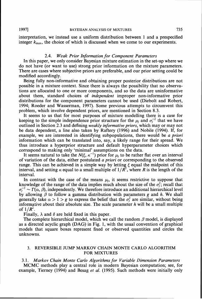
2.4. Weak Prior Information for Component Parameters In this paper, we only consider Bayesian mixture estimation in the set-up where we
do not have (or want to use) strong prior information on the mixture parameters. There are cases where subjective priors are preferable, and our prior setting could be modified accordingly.
Being fully non-informative and obtaining proper posterior distributions are not possible in a mixture context. Since there is always the possibility that no observa- tions are allocated to one or more components, and so the data are uninformative about them, standard choices of independent improper non-informative prior distributions for the component parameters cannot be used (Diebolt and Robert, 1994; Roeder and Wasserman, 1997). Some previous attempts to circumvent this problem, which involve dependent priors, are mentioned in Section 8.3.
It seems to us that for most purposes of mixture modelling there is a case for keeping to the simple independence prior structure for the pj and ay2that we have outlined in Section 2.3 and defining weakly informative priors, which may or may not be data dependent, a line also taken by Raftery (1996) and Nobile (1994). If, for example, we are interested in identifying subpopulations, there would be a priori information which can be translated into, say, a likely range for their spread. We thus introduce a hyperprior structure and default hyperparameter choices which correspond to making only 'minimal' assumptions on the data.
It seems natural to take the N(J, IC-I) prior for p, to be rather flat over an interval of variation of the data, either postulated a priori or corresponding to the observed range. This can be achieved in a simple way by lettin 3J equal the midpoint of this interval, and setting IC equal to a small multiple of l /R , where R is the length of the interval.
In contrast with the case of the means pj, it seems restrictive to suppose that knowledge of the range of the data implies much about the size of the a;;recall that
-. r ( a , p), independently. We therefore introduce an additional hierarchical level by allowing P to follow a gamma distribution with parameters g and h. We shall generally take cu > 1 > g to express the belief that the a? are similar, without being informative about their absolute size. The scale parameter h will be a small multiple of I I R ~ .
Finally, X and S are held fixed in this paper. The complete hierarchical model, which we call the random /3 model, is displayed
as a directed acyclic graph (DAG) in Fig. 1, with the usual convention of graphical models that square boxes represent fixed or observed quantities and circles the unknowns.
3. REVERSIBLE JUMP MARKOV CHAIN MONTE CARL0 ALGORITHM FOR MIXTURES
3.1. Markov Chain Monte Carlo Algorithms for Variable Dimension Parameters MCMC methods play a central role in modern Bayesian computation; see, for
example, Tierney (1994) and Besag et al. (1995). Such methods were initially only

RICHARDSON AND GREEN [No. 4,
Fig. 1. (a) DAG specific to the normal mixture model implemented in this paper; (b) corresponding conditional independence graph
available for problems where the posterior distribution has a density with respect to some fixed standard underlying measure, and so could not be used in cases, such as mixture estimation, where 'the number of things that you do not know is one of the things that you do not know'. Recently, MCMC methods for varying dimension problems have been discussed (Grenander and Miller, 1994; Green, 1994; Phillips and Smith, 1996). One approach, termed reversible jump MCMC, is elaborated in Green (1995), including applications to changepoint analysis in one and two dimensions, and to partition problems arising in Bayesian analysis of factorial experiments. In brief, reversible jump MCMC is a random sweep Metropolis- Hastings method (Metropolis et al., 1953; Hastings, 1970) adapted for general state spaces. Letting x denote the state variable (in our application x is the complete set of unknowns (p,p, CT,k, w, z)), and ~ ( d x ) the target probability measure (the posterior distribution), we consider a countable family of movl types, indexed by m = 1, 2, . . . . When the current state is x, a move type m and destination x' are proposed, with joint distribution given by an essentially arbitrary subprobability measure qm(x, dx'). (With probability 1 - EmJx, qm(x, dx'), no move is attempted.) The move is accepted with probability
{ *(dxl) qm (XI, dx) }am(x, x') = min 1, ~ ( d x )qm(x, dx') '
where the ratio of measures can be given a rigorous definition as a ratio of Radon- Nikodym derivatives with respect to a suitably chosen common dominating measure. The existence of such a measure is ensured by a 'dimension balancing' condition on the qm(x, dx') that effectively matches the degrees of freedom of joint variation of the state and proposal as the dimension changes with k.

19971 BAYESIAN ANALYSIS OF MIXTURES 737
For a move type that does not change the dimension of the parameter, this rather abstract expression reduces to the familiar Metropolis-Hastings acceptance prob- ability, using an ordinary ratio of densities (Hastings, 1970; Peskun, 1973); for dimension-changing moves, a little more care is needed. However, in a typical case, a more concrete form can be given. Suppose that a move of type m is proposed, from x to a point x' in a higher dimensional space. This will very often be implemented by drawing a vector of continuous random variables u, independent of x, and setting x' by using an invertible deterministic function xl(x, u). The reverse of the move (from x' to x) can be accomplished by using the inverse transformation, so that the proposal is deterministic. Then the acceptance probability (6) reduces to
min { 1,
where rrn(x) is the probability of choosing move type m when in state x, and q(u) is the density function of u. Note that the final term in the ratio above is a Jacobian arising from the change of variable from (x, u) to x'.
3.2. Reversible Jump Moves for Normal Mixtures Reversible jump MCMC is most simply derived mathematically in its random scan
form, but as usual with Metropolis-Hastings methods the idea is equally valid when the available moves are scanned systematically, and that is the approach we have chosen to take here.
For our hierarchical normal mixture model, we shall make use of six move types:
(a) updating the weights w; (b) updating the parameters (p, a); (c) updating the allocation z; (d) updating the hyperparameter P; (e) splitting one mixture component into two, or combining two into one; (f) the birth or death of an empty component.
Moves (e) and (f) involve changing k by 1, and making necessary corresponding changes to (p, a, w, z).
The only randomness in the scanning is the random choice between splitting and combining in move (e), or birth and death in move (f). One complete pass over these six moves will be called a sweep and is the basic time step of the algorithm.
All MCMC algorithms make use of the full conditional distributions of some variables given all others, and in deriving these it is helpful to consult the conditional independence graph of the system, derived from the DAG by 'moralizing' and dropping the arrows (Lauritzen and Spiegelhalter, 1988). For our model this graph is displayed in Fig. 1, from which we note that, given all other variables, w and (p, a) are conditionally independent, and similarly for z and P. Moves (a) and (b) can therefore be performed in parallel, and so can (c) and (d).
Move types (a), (b), (c) and (d) are conventional, largely following Diebolt and Robert (1994); they do not alter the dimension of the complete parameter vector (P, p, a, k, w, z), and we shall not give much detail about them here. Through conjugacy,

738 RICHARDSON A N D GREEN [No. 4,
the full conditional distribution for the weights w remains Dirichlet in form:
where nj = #{i: zi =j}, and here and later we use ' 1 . . .' to denote conditioning on all other vanables. Thus w can be updated by a Gibbs move, sampling from this full conditional by drawing independent gamma random variables, and scaling them to sum to 1.
The full conditionals for {p,} are
To preserve the ordering constraint on the {pj}, the full conditional is used only to generate a proposal and is accepted provided that the ordering is unchanged.
The full conditionals for {a;}are
and for the allocation variables we have
whereas the only hyperparameter that we are not treating as fixed, 0,has a gamma distribution
For all these variables, we use a Gibbs kernel. For the split or combine move (e), the reversible jump mechanism is needed. Recall
that we need to design these moves in tandem: they form a reversible pair. The strategy is to choose the proposal distributions according to informal considera- tions suggesting a reasonable probability of acceptance, but strictly subject to the requirement of dimension matching. Having done so, conformation with the detailed balance condition is determined by the acceptance probability (7). This is the point at which the statistical model is used quantitatively.
In move (e), we make a random choice between attempting to split or combine, with probabilities bk and dk = 1 - bk respectively, depending on k . Of course, dl =0 and bk,,, = 0, where kmaxis the maximum value allowed for k , and otherwise we choose bk = dk =0.5, for k = 2, 3, . . ., kmax- 1 . Our combine proposal begins by choosing a pair of components GI,j2) at random, that are adjacent in terms of the current value of their means, i.e.
PJI < Pj~iz~ with no other pj in the interval [p,, ,pI2]. (9)
These two components are merged, reducing k by 1. In doing so, forming a new
19971 BAYESIAN ANALYSIS OF MIXTURES 739
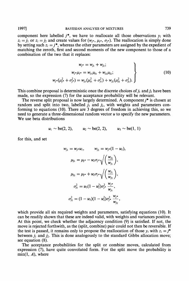
component here labelled j*, we have to reallocate all those observations yi with zi=jl or zi=j2and create values for (wj*, k*,aj*). The reallocation is simply done by setting such zi =j*, whereas the other parameters are assigned by the expedient of matching the zeroth, first and second moments of the new component to those of a combination of the two that it replaces:
This combine proposal is deterministic once the discrete choices of jl andj2have been made, so the expression (7) for the acceptance probability will be relevant.
The reverse split proposal is now largely determined. A component j* is chosen at random and split into two, labelled jl and j2, with weights and parameters con- forming to equations (10). There are 3 degrees of freedom in achieving this, so we need to generate a three-dimensional random vector u to specify the new parameters. We use beta distributions
for this, and set
which provide all six required weights and parameters, satisfying equations (10). It can be readily shown that these are indeed valid, with weights and variances positive. At this point, we check whether the adjacency condition (9) is satisfied. If not, the move is rejected forthwith, as the (split, combine) pair could not then be reversible. If the test is passed, it remains only to propose the reallocation of those yiwith zi=J*
between jl and j2. This is done analogously to the standard Gibbs allocation move; see equation (8).
The acceptance probabilities for the split or combine moves, calculated from expression (7), have quite convoluted form. For the split move the probability is min(1, A), where

RICHARDSON AND GREEN
6-I+/! 6-l+h
A = (likelihood I) (k + 1) W ~ ' W ~ 2+
6- 1+/I +I2P(k) wj* B(6, kS)
where k is the number of components before the split, lI and l2 are the numbers of observations proposed to be assigned to jl and j2, B(., .) is the beta function, Pan, is the probability that this particular allocation is made, g , , denotes the beta(p, q) density and likelihood ratio is the ratio of the product of the f(yilO,,)-terms for the new parameter set to that for the old. For the corresponding combine move, the acceptance probability is min(1, A-I), using the same expression for A but with some obvious differences in the substitutions.
The correspondence between expressions (7) and (1 1) is fairly straightforward; the first three lines of expression (1 1) form the ratio p(xfly)/p(xly), the (k + I)-factor in the first line being the ratio (k + l)!/k! from the order statistics densities for the parameters (p, a2). The fourth line is the proposal ratio rm(xf)/rm(x)q(u), and the final
2 2line is the Jacobian of the transformation from (wj*, pj*, gj*, MI, 242, 243) to (wjl, pjl, ajl, 2
Wj2, Pj2, ~j2). The birth-and-death move (f) is somewhat simpler. We first make a random choice
between birth and death, using the same probabilities bk and dk as above. For a birth, a weight and parameters for the proposed new component are drawn using
wj* - be(1, k), pj* -N(6, K-'), - r(a,p). To 'make space' for the new component, the existing weights are rescaled, so that all weights sum to 1, using wj = wj(l - wj*). For a death, a random choice is made between any existing empty components, the chosen component is deleted and the remaining weights are rescaled to sum to 1. No other changes are proposed to the variables: in particular, the allocations are unaltered.
Detailed balance holds for this move, provided that we accept births and deaths according to expression (7), in which (wj*, pj*, aJ<) play the role of u. The use of the prior distributions in proposing values for pJ* and gj*leads to a simplification of the resulting ratio. The acceptance probabilities for birth and death are min(1, A) and min(1, A - I ) respectively, where

19971 BAYESIAN ANALYSIS OF MIXTURES 741
Here, k is the number of components and ko the number of empty components, before the birth. In equation (12), the first line is the prior ratio, and the second line contains the proposal ratio and Jacobian; the likelihood ratio is 1.
This completes the specification of the moves, which we do not claim is optimal; indeed, this is almost the first scheme that we tried. The validity of the algorithm is not compromised by the choice of proposals, since detailed balance is confirmed by using expression (7). In Metropolis-Hastings methods, it is rarely worth fine-tuning the proposal distribution, especially if doing so prevents simple and explicit random variate generation.
With detailed balance satisfied, it only remains to check that the Markov chain defined is irreducible and aperiodic. Aperiodicity is clear, since given any arbitrarily small neighbourhood of a current state (P, p, a, k, w, z) there is positive probability that after one sweep through moves (ak(f) the chain lies in that neighbourhood. Irreducibility is also easily established, since the chain can move from any value of k to any other value in steps of one at a time, in move (c) all allocations have positive probability and the parameters and hyperparameters are updated by drawing from continuous distributions whose supports are the natural parameter spaces.
4 . STATISTICAL PERFORMANCE OF METHODOLOGY PROPOSED
Several interlinked aspects of the methodology proposed are to be demonstrated in illustrating its performance. Of course, we display examples of the results that we obtain from real data sets. But the presentation of substantive results is inevitably associated with questions of sensitivity to model specification, especially regarding the prior, and questions about the performance of the MCMC sampling method, i.e. how well it 'mixes'. These three aspects-results, sensitivity and mixing-interact closely. To avoid circularity in our presentation, we postpone discussion of sen- sitivity and mixing to Sections 5 and 6 respectively, and first present a description of the performance of the model itself with default settings for the hyperparameters. Of course, sensitivity issues informed our choices here.
4.1. Results for Three Data Sets Three real data sets are used throughout the paper, as a basis for our com-
parisons. (All three data sets can be obtained from the World Wide Web at h t t p : / / W W W . s t a t s .b r i s . a c . u k / - p e t e r / m i x d a t a . ) The first concerns the distribution of enzymatic activity in the blood, for an enzyme involved in the metabolism of carcinogenic substances, among a group of 245 unrelated individuals. The interest here is in identifying subgroups of slow or fast metabolizers as a marker of genetic polymorphism in the general population. This data set has been analysed by Bechtel et al. (1993), who identified a mixture of two skewed distributions by using maximum likelihood techniques implemented in the program SKUMIX of Maclean et al. (1976). We shall refer to this data set as the 'enzyme data'. The second data set, the 'acidity data', concerns an acidity index measured in a sample of 155 lakes in north-central Wisconsin and has been previously analysed as a mixture of Gaussian distributions on the log-scale by Crawford et al. (1992, 1994); we also use the log-scale. The last data set, the 'galaxy data', was first described in Roeder (1990) and subsequently analysed under different mixture models by several researchers

742 RICHARDSON A N D G R E E N Wo. 4,
including Escobar and West (1995) and Phillips and Smith (1996). It consists of the velocities of 82 distant galaxies, diverging from our own galaxy. Histograms of the three data sets are shown in Fig. 2.
The three data sets have been analysed with the hierarchical normal random P mixture model defined in Sections 2.3 and 2.4, with the following settings for previously unspecified constants: K - 1/R2, cr = 2, g = 0.2, h = 10/R2 and S = 1. The prior on k is taken as uniform on the integers 1,2, . . ., k,,, = 30, for which it is particularly easy to convert results to those corresponding to other priors on these values, using the identity
where p*(.ly) denotes the posterior for an alternative prior p*. For each of the three data sets, we report results corresponding to 100000 sweeps,
following a burn-in period also of 100000 sweeps. We believe that these numbers
10 15 20 25 30 35 (C)
Fig. 2. Predictive densities for (a) the enzyme, (b) the acidity and (c) the galaxy data sets, unconditionally (-------) and conditionally (-- --) on various values of k: the curves displayed are for k - 2 4 , except for the galaxy data, where they are for k = 3-6; in each case note that it is only the srr~allestk shown that gives an appreciably different estimate

19971 BAYESIAN ANALYSIS OF MIXTURES 743
TABLE 1 Posterior distribution of k for the three data sets based on a mixture model with random /3 and default?
parameter values
Data set n Proportion (%) of moves accepted
Split- Birth-combine death
Enzyme 245 p(1) =0.000 p(5) = 0.206 p(9) =0.007
Acidity 155 p(1) =0.000 p(5) =0.172 p(9) = 0.020 p(13) =0.001
Galaxy 82 p(1) =0.000 p(5) =0.182 p(9) =0.071 p(13) = 0.006
?Range and default parameter values: enzyme data, R = 2.86, J = 1.45, K =0.122, cr = 2, g = 0.2, h = 1.22, 6 = 1 ; acidity data, R = 4.18, J = 5.02, K = 0.057, cr = 2, g = 0.2, h = 0.573, 6 = 1 ; galaxy data, R = 25.1 1 , J = 21.73, K =0.0016, cr = 2, g = 0.2, h = 0.016, 6 = 1 .
exceed what is needed for reliable results. In all the runs, the number of components never exceeded 24; hence the chosen value of k,,, was inconsequential.
Estimated posterior probabilities are given in Table 1. In each of the data sets, it is immediately apparent that there are several competing explanations of the data which are tenable. For the enzyme data, the posterior for k favours 3-5 components. In this example, with the proviso that there is some prior evidence for enzyme level to be normally distributed, we could interpret the existence of three components in the mixture in terms of a simple underlying genetic model. For the acidity data, there is again fairly equal support for 3-5 components; for the galaxy data, the posterior for k is more widely spread and indicates a higher number of components, between 5 and 7. In each case, the high overall number of components can be related in part to the skewness of the data, two or three normals being sometimes needed to fit one skewed component, but also to our mixture model which imposes little structure a priori, in contrast with those considered by Roeder and Wasserman (1997) or Gruet et al. (1 996).
As a by-product of our implementation, we can also investigate changes in the posterior distribution of 'deviances' -2 logp(ylk, w, 8) for increasing k. For the enzyme data, there is a marked shift between k = 2 and k = 3, whereas from k = 3 onwards there is substantial overlap between the deviance distributions; see Fig. 3(a). A similar pattern emerges for the other two data sets, with substantial overlap from k = 3 for the acidity data and from k = 4 for the galaxy data.
4.2. Predictive Densities At each sweep of the algorithm, values (w, 8) of the weights and parameters are
produced, from which densities

744 RICHARDSON AND GREEN [No. 4,
deviances (a)
10 20 30 40 data
(b)
Fig. 3. (a) Posterior distributions of deviances for the enzyme data (-, k = 2; .........., k = 3 ; - - - -,k = 4; ----, k = 5 ; --, k = 6); (b) sample from the posterior distribution of f ( . lk , w , 8) for the galaxy data
can be computed. Posterior variation among the realized f(.lk, w, 9) is displayed in Fig. 3(b), for the galaxy data.
Averaging the f(.lk, w, 8) across the MCMC run, conditionally on fixed values of k , gives an estimate of E{f(.lk, w, 9)lk, y } , a Bayesian predictive density estimate of

19971 BAYESIAN ANALYSIS OF MIXTURES 745
the mixture with k components. Averaging further across values of k gives an estimate of E{ f(Ik, w, 8)ly), the 'overall' Bayesian predictive density estimate of the distribution of y. Note further that these density estimates do not themselves have the shape of a finite mixture of distributions. Other density estimates, in particular the mixtures f(.Ik, G, 8) for each k, have been considered, where G and 8^ are summary posterior estimates of the weights and parameters of a k-components mixture. In the case where the posterior distribution of (w, 8) is fairly spread out or even multimodal, these plug-in estimates would give a poor oversmooth approximation of the pre- dictive density.
Predictive densities, both conditional on k and unconditional, are shown in Fig. 2 for the three data sets. Note that the difference between successive predictive densities decreases with increasing values of k and that the overall unconditional plot gives a convincing density estimate of the data distribution. The predictive fit and posterior distribution give complementary evidence on which to draw when assessing the number of components. For the enzyme data, the predictive plots for three or four components are very similar. Since one aim of the analysis of this data set is the identification of interpretable subpopulations, we would favour the mixture with three components.
4.3. Parameter Estimates 4.3.1. Labelling and post-processing Markov chain Monte Carlo output
Although it is in some ways natural to consider the parameters as a set, labelling at each sweep is convenient and becomes necessary when density estimates or other summaries of the posterior distribution of the parameters of each component are required. The most appropriate labelling will depend on the example analysed and it is a substantial bonus of the sample-based computation method we use that this can be investigated after the run of the algorithm.
To understand why the issue of labelling is not straightforward, consider the case where the population is really of two normal components, unambiguously labelled. Given a finite sample, the posterior distribution of the two means will overlap, and similarly for the weights and variances; the extent of the overlaps depends on the separation and the sample size. When the means are well separated, labelling of the realizations from the posterior by ordering their means will generally coincide with the population labelling; as the separation reduces, so-called 'label switching' will occur; see also Mengersen and Robert (1996). Depending on the relative separations, label switching can be minimized by choosing to order on the variances, weights or some combination of all three parameters.
We illustrate these points in Fig. 4 by using a simulated data set of n = 250 points, drawn from a mixture which gives a skewed unimodal distribution (wl = w2 = 0.5; p1 = 0.0; p2 = 1 .O; a1 = 1.5; a 2 = 1.0). Fig. 4(a) displays the posterior densities of w,, and pj and aj for the runs where k = 2, for a labelling corresponding to an ordering of the means and Fig. 4(b) for a labelling corresponding to an ordering of the variances. The labelling according to the variances (Fig. 4(b)) leads to bimodal densities for pj, j = 1,2, which corresponds to label switching on about half the runs. Labelling by ordering the means gives clearer unimodal plots simultaneously for all three parameters, with still some evidence of switching. In a real data set, there might not be an obvious choice of labelling. It is then advisable to post-process the run

746 RICHARDSON AND GREEN [No. 4,'I' 2
00
00 0 2 04 0.6 0.8 1 0 weights
means means means means
Fig. 4. Posterior density of parameter estimates for two choices of labelling, simulated data sets: (a) labelling according to ordering of the means; (b) labelling according to ordering of the variances
according to different choices of labels to obtain the clearest picture of the component parameters.
4.3.2. Multimodality of parameter densities Quite apart from the labelling problem, there might be cases of genuine mul-
timodality of the posterior distribution of parameter estimates corresponding to different mixture models competing for potential explanations of the data set.
As an example we display in Fig. 5 (full curve) the posterior densities for the weights and the means of the second and third component for the enzyme data (with labels according to the ordering of the means). There is some evidence of bimodality in the distributions of the weights for the second and third components. Different labelling does not help to clarify the picture. In an attempt to exhibit possible competing explanations, we separate out in the MCMC output those runs corresponding to w3 ,< 0.17 and plot the parameter densities again (dotted curves in Fig. 5). This produces more clearly peaked posterior densities for all the param-eters, and shows that low values of w3 are associated with elevated values of p3. In fact, a further separation according to w3 < 0.05 would show that this small group

19971 BAYESIAN ANALYSIS OF MIXTURES 747
0.0 0.2 0.4 0.6 0.8 1.0 0.0 0.2 0.4 0.6 0.8 1.0 weights weights
0
0.0 0.5 1 .O 1.5 2.0 2.5 0.0 0.5 1.0 1.5 2.0 2.5 means means
Fig. 5. Enzyme data set: posterior densities of weights and means for the second and third component, default prior model, conditioning on k = 3 (-), and conditioning also on wj < 0.17 (..........) and on w3 > 0.17 (- - - -) (the last two have areas proportional to the posterior probability)
corresponds to p3 2 2.0, indicating that only a small fraction of individuals have high enzymatic activity, as expected.
5 . SENSITIVITY OF RESULTS TO PRIOR ASSUMPTIONS
Our hierarchical approach to mixture modelling involves hyperparameter speci- fications. We have carried out a detailed study of their influence which has led us to make the standard default recommendations that we have used in the previous section. In this section, we highlight some important aspects of our sensitivity analysis. We emphasize that we do not recommend that such a study should be performed for a standard implementation of our approach!
5.1. Sensitivity of Posterior Distribution of k 5.1.1. Comparison of prior models for the variance: fixed versus random P
Our main concern here is to show how, in our model, the number of components is related to the prior information on the variances a;. In the standard non-hierarchical model with fixed P and cu the mean of the gamma distribution, a l p , specifies the typical value of the precision a;*. It is natural to relate ojto the range R of the data and increasing values for J(P/cu) will lead to models with fewer components. In Fig. 6(a) we show, on the acidity data, the substantial change in the posterior distribution of k as J(P/cu) is varied between R/5, R/lO and R/20. There is little overlap between the posterior distributions of k for the two extreme cases. Hence, in the standard model, the choices of a and P will crucially influence the posterior distribution of k and it is difficult to be weakly informative.
In contrast, the hierarchical model with fixed a but random P that we have

RICHARDSON AND GREEN [No. 4,
Fig. 6. Posterior distributions of k: comparison of sensitivity to hyperparameters between fixed and random p models: (a) fixed P, a = 2 and +/@/a)varying between R/5 (-), R/10 (..........) and R/20 (- - - -); (b) random p, a = 2, g = 0.2 and &/ha) varying between R/5 (-), R/10 (........-) and R/20 (- - - -)
implemented, which allows weak information on ajto be put in at a higher level, does not exhibit the same behaviour. The posterior distribution of k is quite insensitive over a wide range of values of the ratio g/h (related again to the range R) which all lead to a similar posterior mean and standard deviation for P. This is well illustrated in Fig. 6(b) which shows strikingly similar posterior distributions for k for three sets of values for a , g and h chosen so that the prior order of magnitude for aj at the higher level, J(g/ha), ranges again from R/5 to R/20. Hence our hierarchical for- mulation for the variance distribution in the mixture model allows a high degree of non-informativeness. It is in view of these results that we choose the hierarchical random p model with a =2, g = 0.2 and J(g/ha) = R/10 as our default option.
5.1.2. Sensitivity to prior distribution of means An important component of the mixture model is the prior model for the means p,,
which we defined as drawn independently from the normal distribution N(J, n-I). Using only the extremes of the data we consider that setting 6 equal to the mid- range and the precision n so that n-lh is equal to R is a sensible weakly informative prior which places effectively no constraint on the location of the pi but does not encourage the fitting of mixtures with very close p,.
There is a subtle interplay between prior information on the location of the means and the number of components. Indeed reducing n-'I2 at first will tend to favour a higher number of components. This can be interpreted as the result of defining a prior for the means which is increasingly more permissive of components with close means. However, as n-'I2 is further reduced, the number of components will start to decrease, as there is now a shrinkage effect and active prohibition of components with means located towards the extremes of the range. We illustrate these points on the acidity data. We have used throughout the same hierarchical default option for the variances, but a Poisson prior P(10) for k as some hyperparameter settings now encourage large k. As the values of n-'I2 decrease from R to R/10, the number of components with the highest posterior probability first increases to reach a peak value of k = 10 for ti-'I2 between R/4 and R/5 and then decreases again (Table 2).
We have so far discussed sensitivity to the prior setting of K, with the hierarchical random p model for the component variances, but the same behaviour is observed

19971 BAYESIAN ANALYSIS OF MIXTURES
TABLE 2 Influence of prior distribution N(6, K - I ) for p on the posterior
distribution of kt
&-I12 Range of k with k with highest p ( k ) p fk ly ) 2 0.05 p(kly) 2 0.001
R [3-91 [2- 1 31 6 R / 2 ($121 [3-171 8 R / 3 [&I41 [4-191 9 R / 4 [7- 1 41 [3-2Ol 10 R / 5 [7-141 [4-201 10 ~ 1 8 ~ - 1 2 1 [3-171 8 R / ~ O [ 4 - 1 1 1 [3-161 7
?Acidity data: mixture model with Poisson (prior P(10) for k), random P and default parameter values o;* - r ( 2 , p), 0- r (0 .2 , h ) with , /&/ha) = R/10 .
with the fixed P model. Sensitivity was discussed by Crawford (1994) who computed, for the acidity data, the posterior distribution of k in three cases: cr = P = K, = 1, cr = p = K, = 5 and cr = ,O = K, = 10. Note that the restriction imposed on the means is quite severe in the last two cases, K, = 1, 5, 10 corresponding respectively to equal to R/4, R/10 and R/13 for this data set. By simultaneously increasing a , ,8and K,, the means of the components are restricted, whereas the standard deviations are tightened around 1 * R/4, a fairly large value, thus creating competing influences on k which are not easy to disentangle. We have fitted our model with the same parameter settings as Crawford. We find more support for two components than in our previous analysis with our default priors (see Table I), a posterior distribution mostly concentrated on k = 2 or k = 3, with moderate variation between the three cases, p(k = 21y) being equal to 0.42, 0.65 and 0.43 respectively. However, the Laplace approximation estimates for p(k = 2(y) given in Crawford's Table 2 vary over many orders of magnitude.
5.2. Sensitivity of Posterior Distributions of Parameters In a complementary way and from the same MCMC runs, we can investigate the
sensitivity of the posterior distributions of component parameters for various values of k. We shall briefly summarize some features.
Results concerning the influence of K, are unsurprising. As expected, a reduction in the range of the means pj is observed as K , - ' / ~ is decreased, something which is more noticeable for large k.
It is interesting to compare the influence of prior specifications for the variances a,-2 - r (a , p) between the fixed P and the random ,8- r(g, h) model. A similar sensitivity pattern to that described for the posterior distribution of k emerges. In the fixed P case the posterior means of aj are sensitive to variations in ,/(/?/a), the more so when k is larger. For example, for the acidity data with k = 4, the posterior means of a, become nearly halved as J(P/a) is varied from R/5 to R/20, whereas for the random ,B case all the posterior means of a, are remarkably similar. This is further evidence for the value of including an upper hierarchical level in the distribution of the a, in a mixture model.

750 RICHARDSON AND GREEN [No. 4,
6. PERFORMANCE OF MARKOV CHAIN MONTE CARL0 SAMPLER
6.1. Mixing over k: Performance of Jump Moves An essential element of the performance of our MCMC sampler is its ability to
move between different values of k. A plot of the changes in k against the number of sweeps for the galaxy data is presented in Fig. 7 . It shows that the MCMC algorithm mixes well over k, excursions into very high values being short lived. Similar plots were obtained for the other data sets. Proportions of accepted 'split or combine' moves vary between 8% and 14% (Table 1 ) . For dimension-changing moves, these proportions are satisfactory and show that our proposal based on adjacency is sensible. A useful check on the stationarity is given by the plot of the cumulative occupancy fractions for different values of k against the number of sweeps. These are represented in Fig. 7 for the three data sets, where it can be seen that the burn-in is more than adequate to achieve stability in the occupancy fractions.
Our model does not preclude empty components, and they will be included in our count of k . This might cause concern if a high number of them persisted for long times. We have found that including in our algorithm the birth-death moves, which specifically deal with empty components, improves convergence in comparison with that of an algorithm relying only on the split or combine moves, especially when the posteriors are diffuse. The acceptance rate for birth-and-death moves is highest for the small and multimodal galaxy data set. The mean number of empty components is equal to 0.10, 0.18 and 0.57 for the enzyme, acidity and galaxy data sets respectively.
We detected no influence of starting values on the distribution of k . For example, with the enzyme data, starting with k = 1 typically leads to the acceptance of the first
sweep sweep (a) (b)
sweep sweep (C) (d)
Fig. 7. (a) Example of a trace of k for the galaxy data set, for 50000 sweeps after bum-in, and cumulative occupancy fractions for (b) the galaxy, (c) the enzyme and (d) the acidity data sets, for a complete run including bum-in

19971 BAYESIAN ANALYSIS OF MIXTURES 751
split after fewer than five sweeps, and then k = 1 is never accepted again; further, when starting with k =20, and observations ranked then equally allocated between the components, fewer than 100 sweeps are needed to reach k = 10. Unless specified otherwise, all our runs start with k = 1.
The prior distribution of k, p(k), appears in the acceptance ratio for the dirnension- changing moves and will influence the mixing behaviour precisely through that ratio. Priors which are highly concentrated on a range of values of k will effectively stop the algorithm from accepting moves which will take it outside this range. However, the Bayes factors
which are theoretically independent of p(k), have MCMC estimates that are not materially affected by it, within the range of k visited reasonably often. For example, on the acidity data, B34is estimated as 0.91, 0.99 and 1 .O1 when the prior for k is a Poisson distribution with mean equal to 1, 3 and 10 respectively and as 1.03 for a uniform prior for k (between 1 and 30).
6.2. Mixing within k 6.2.1. Within-k mixing for parameters
Within the range of weak priors that we have been using, we have observed satisfactorily mixing patterns in all our runs and not encountered any 'trapping states' as reported in Robert (1996). We checked that runs with very different initial allocations gave almost identical posterior densities for the parameters. For the enzyme data and three components, Fig. 8 displays typical time plots of the sweeps for w, p and a. These are based on a run of 100000 sweeps, which included about 30000 visits to k = 3, but plotted only every 20 for clarity in these plots. Different patterns of traces for the three components can be seen. The first component (low- est mean and standard deviation, highest weight) is estimated precisely. Very occasionally, much fewer than 60% of the observations are allocated to it, but this creates no problem. When this occurs, the mean of the second component dips as some switching arises between the two components. The weights of the second and third components are more fluctuating. For the third component, competing explanations, as discussed earlier in Section 4.3.2, are clearly visible and the algorithm has no trouble in covering the wider range of values, higher means corresponding to lower weights and standard deviations.
6.2.2. Comparisons with $xed k sampler Some previous work using the MCMC method in mixture estimation with fixed k
has encountered slow mixing, especially with weak priors. This is usually caused by two or more modes in the posterior distribution, separated, as far as the available MCMC moves are concerned, by regions of low probability. In statistical terms, there are two or more well-supported explanations for the data with the same k. For example, the data may fall into two rather well-separated clusters, and with k fixed at 3 there may be substantial posterior probability on two components being fitted to the first cluster and one to the second, or vice versa.
It is plausible that, in the presence of multimodality, mixing should be improved

752 RICHARDSON AND GREEN [No. 4,
0 5OM) 1 m 1 5M)O MWO 2 m sweep
0 SOM) lW00 1 m 2W00 25000 sweep
0 5WO IWM) 15000 2W00 25WO sweep
Fig. 8. Traces of parameter estimates against visits to k = 3, enzyme data
by the possibility of varying k. In the particular situation described above, the sampler could, at some stage, combine the two components in the first cluster and subsequently split the component in the second cluster, and so complete a transition from one mode to the other, without visiting regions of low posterior probability. This is an example of what physicists would call 'tunnelling' between regions of low 'energy' (energy is the negative logarithm of the probability).
Here we present an example of the improved mixing obtained by varying k. The example is somewhat contrived, but we believe that it is qualitatively similar to real problems with clustered data, in the absence of strong prior information. We take 50 observations from N(2.5, I), 50 from N(4, 1) and assemble a synthetic data set of size 200 by taking these 100 data points and their reflections about the origin. Our default prior is used, except that k is given a Poisson prior, with X = 4. We thus contrive a situation in which the joint posterior distribution has exact symmetry on reflection about 0. We compare results of simulating the joint posterior with variable k, and then conditioning on k = 3, with running a fixed k sampler for k = 3 using only moves (a t (d) of Section 3.2. Run lengths were arranged so that the same numbers of visits to k = 3 were made in each case. Some results are displayed in Fig. 9. By symmetry, the true posterior p(p21y, k = 3) is symmetric about 0, and in particular p(p2 < OIy, k = 3) = 0.5. Figs 9(a) and 9(c) show traces of p2 against sweep number. The variable k sampler evidently mixes far better than the fixed k sampler. This

19971 BAYESIAN ANALYSIS OF MIXTURES
8 0 1000 2000 3000 4000 5000 6000 -4 -2 0 2 4
sweep PZ (a) (b)
8 0 1000 2000 3000 4000 5000 6000 0 1000 3000 5000
sweep sweep (c) (d)
Fig. 9. Comparison of mixing of variable k and fixed k samplers: (a), (c) traces of p2 against sweep number; (b) posterior density estimates at the end of the runs; (d) sequences of estimates of p(p2 < Oly, k = (-, obtained as the runs proceed 3) variable k sampler)
improvement extends to estimates of the density of p2 and the probability that it is positive, illustrated in Figs 9(b) and 9(d). After more than 6000 sweeps, results for the fixed k sampler still show severe asymmetry.
7. BAYESIAN CLASSIFICATION
Apart from their role in facilitating computation, the allocation variables z are of interest in their own right, for they form a coherent basis for classification of the observaiions. Some care is required in interpreting these sensibly. It will rarely be appropriate to discuss classification except conditionally on k, and even then the labels 1, 2, . . ., k are only meaningful in the context of some particular declared unambiguous labelling of the k mixture components, e.g. by ordering on the p,.
Classification can either be done on a within-sample or a predictive basis. For the former, the posterior probabilities @(zi =jly, k); j = 1, 2, . . ., k) are appropriate, and these can be directly estimated as empirical averages in the MCMC run. Predictive classification addresses the question of classifying a future observation y*, say. If the allocation variable corresponding to this is z*, then we are in principle interested in @(z* =jly, y*, k)). Unfortunately, inclusion of the additional datum changes all the posterior distributions, apparently requiring that the MCMC sampler be rerun for each new y*! This is obviously impractical, so we employ the obvious approxima tion

754 RICHARDSON AND GREEN WO.4,
= IP(Z* =jly*, k, 8, w)p (~ ,wiy, y*, k ) d ~ d w
and estimate the last integral, like any other expectation with respect to p(8, wly, k), by an MCMC empirical average, in this case that of
where 4(.; p, o) is the normal density. In Fig. 10, the estimated within-sample and predictive classification probabilities are illustrated for the enzyme data set. The lower section of each part shows the cumulative classification probabilities p(zi <jly, k) and p(z* <jly, y*, k) for j = 1, 2, . . ., k - 1; differences between adjacent curves indicate the class probabilities. The within-sample probabilities and the predictive probabilities coincide to within plotting accuracy. This is an effect of the law of large numbers; they are computed separately.
Using the usual 'percentage correctly classified' loss function, the Bayes classifica-tion of an existing observation yi and a future one y* are respectively given by
h
Z = argmax Ip(zi =jly, k)) and z* = argmax Ip(z* =jly, y*, k)}. j j
These are also plotted, in the upper part of each panel, in Fig. 10. Note that there is no monotonicity in the classification with respect to increasing
values of the enzyme level. For k = 3, data values classified to the third component lie on either side of those assigned to the second component. This is due to the large variance of the third component. Correspondingly, the predictive curve delimiting
w . ?, . N ---9.-m
-ad-P
w 0
2 -
0. 0
dala data data
(a) (b) (c)
Fig. 10. Classificationsof the enzyme data set: within-sample ( +) and predictive (------) classification probabilities and optimal classifications for (a) k = 2, (b) k = 3 and (c) k = 4

19971 BAYESIAN ANALYSIS OF MIXTURES 755
the second from the third component has a pronounced dip. This phenomenon persists with larger k, indicating that the classifications cannot be simply interpreted in terms of shifts of the mean enzyme level, but take into consideration a combina- tion of mean and spread.
8. FURTHER WORK AND DISCUSSION
8.1. Markov Chain Monte Carlo Issues The key idea in constructing an effective MCMC sampler is to design sensible
moves that use current knowledge about the mixture. Basing moves on a notion of adjacency has a generic character, independent of the particular distributional assumptions, and thus these move types could be adapted to a variety of dis- tributions. We believe that they would be suitable for any two-parameter density f(.lO,, e2),where after a suitable transformation f could be reparameterized in terms of a mean and variance parameter with the range of the mean unconstrained.
We could have extended our birth-and-death moves to include non-empty com- ponents, similarly to Phillips and Smith (1996), and then dispensed with our split and combine moves, or defined combine moves with respect to the underlying partition given by the data rather than the parameters, along the line followed by Gruet et al. (1996). We felt that these moves would be less efficient, but in further developments of our work we aim to perform some comparisons. More adventurous moves could be contemplated, e.g. moves that combine three components or take two components and simultaneously update the relevant parameters, weights and allocations. How- ever, there is no evidence from our results that such complications are necessary.
Although adjacency and preserving the first two moments are quite natural conditions in a one-dimensional setting, the moves thus created might be too restricted for good mixing in applications to bivariate or multivariate mixtures. There, we feel that the algebra of moves will need to be extended.
In calculating the acceptance ratios for dimension-changing moves, the only term which might be cumbersome is the Jacobian of the transformations. In higher dimensional parameter space, symbolic computation tools could be useful at this point. These calculations are simplified by preserving as much symmetry as possible in the definition of the moves.
The intricacy of our MCMC sampler may convey an impression that it is compu- tationally demanding. In fact, the burden is not excessive. For the largest of our three real data sets, the enzyme data, with n = 245, and using the default prior setting, our program makes about 160 sweeps per second on a Sun SPARC 4 workstation.
Validation of the MCMC code is an important concern. We have compared our results with analytic calculations on very small data sets and found a good correspondence. We have also checked that without any data our estimate of the joint posterior distribution tallies with the chosen prior.
8.2. Presentation of Posterior Distributions Extracting information from such a complex multidimensional posterior distribu-
tion is a challenge. Although MCMC methods circumvent the restrictions of conventional numerical methods and provide all the raw information, insightful and disciplined summaries are needed, adapted to the particular context. In the paper we

756 RICHARDSON A N D GREEN [No. 4,
have exploited some opportunities, involving relabelling, predictive densities, classification, etc. New summaries, especially regarding joint parameter distributions, should be developed. Post-processing is especially useful in view of the inherent identifiability problems connected with mixture estimation, which are crystallized in the contrast between the variability of parameter estimates plots, representing competing explanations, and the stability of predictive density plots.
Our approach has revealed clear evidence of multimodality and skewness in posterior distributions, features whose presence is unsurprising in view of the small numbers of observations sometimes allocated to some components. We believe that this is a situation where using analytic approximations such as the Laplace approx- imation can be misleading.
8.3. Other Prior Structures The interaction between the model and the number of components, in terms of
both structural and functional characteristics of the prior, has been discussed and illustrated extensively. We believe that the hierarchical prior structure that we have introduced will be useful for many examples. Nevertheless, it is certainly not a black box procedure. Our default choice for hyperparameters is aimed at using mixtures for analysing heterogeneity rather than for semiparametric density estimation.
A relationship between the prior distribution of the means and the posterior for k is to be expected, and indeed we have found sensitivity to values of 6.Instead of considering the {p,} to be independent, it might be more natural to model the notion of separation of the means explicitly by using dependent priors. This is one example of a feature which could be built into a joint prior distribution for {p,, a?},for which our computational approach would still be available.
Dependent priors over the component parameters have been considered by several researchers when attempting to be non-informative in the mixture context. This essentially entails linking the components via global parameters, to which flat priors can be assigned since all the data points contribute to their estimation. Related but distinct approaches following this line are taken by Robert (1996), Mengersen and Robert (1996) and Gruet et al. (1996), scaling with respect to the component with largest variance, and Roeder and Wasserman (1997), placing Markov priors on the means.
8.4. Generalizations of the Model Among related models to which we have extended our MCMC sampling strategy
is the Escobar and West (1995) mixture model based on a Dirichlet process prior. The hierarchical structure is now somewhat different from that of equation (9,but the range of moves that are needed is broadly the same, and the elegant algebraic structure of the Dirichlet process model facilitates the evaluations needed to implement the split or combine moves.
Our approach has so far been implemented only for normal mixtures, and the interpretation of the number of components is conditional on this being an appropriate distribution for all the subpopulations. If we take any phenotypic data like the enzyme data, the assumption of normality might not be supported by biological considerations. Indeed, the maximum likelihood procedure SKUMIX of

19971 BAYESIAN ANALYSIS OF MIXTURES 757
Maclean et al. (1976) for analysing mixtures does allow for different degrees of skewness through the use of a Box-Cox transformation, and in the original analysis of the enzyme data Bechtel et al. (1993) concluded that the data were fitted by two highly skewed components. One extension that we are considering is the development of a framework where variable numbers of components and variable skewness in the mixture distribution would be simultaneously considered.
Another straightforward extension is to consider mixtures of discrete distributions, a model which is commonly used in nonparametric estimation and which is usually estimated via the EM algorithm separately for different numbers of mass points.
Finally we emphasize the flexibility of our modelling for incorporating many of the extensions which arise when mixture estimation is used in different application contexts. In particular we aim to consider problems involving constraints on the weights for genetic analysis, modelling component means in terms of covariates and using mixtures for robust prior modelling in Bayesian analysis and for modelling unknown exposure distributions in measurement error problems.
ACKNOWLEDGEMENTS
We wish to thank Jim Berger, Ed George, Agostino Nobile, Christian Robert, Kathryn Roeder, Duncan Thomas and Larry Wasserman for stimulating discussions about this work, Catherine Bonaiti for introducing us to the genetic applications of mixture estimation, Pierre Bechtel for providing the enzyme data set, Christine Monfort for assistance with the computations and the referees for suggestions which improved the presentation. We acknowledge the financial support of the Engineering and Physical Sciences Research Council Complex Stochastic Systems Initiative (PJG), the Institut National de la Santt et de la Recherche Mtdicale (SR) and the European Science Foundation Network on Highly Structured Stochastic Systems.
REFERENCES
Bechtel, Y. C., Bonaiti-Pellik, C., Poisson, N., Magnette, J. and Bechtel, P. R. (1993) A population and family study of N-acetyltransferase using caffeine urinary metabolites. Clin. Pharm. Therp., 54, 134-141.
Besag, J., Green, P. J., Higdon, D. and Mengersen, K. (1995) Bayesian computation and stochastic systems (with discussion). Statist. Sci., 10, 3-66.
Celeux, G., Chauveau, D. and Diebolt, J. (1996) Stochastic versions of the EM algorithm: an experimental study in the mixture case. J. Statist. Computn Simuln, 55, 287-314.
Crawford, S. L. (1994) An application of the Laplace method to finite mixture distributions. J. Am. Statist. Ass., 89, 259-267.
Crawford, S. L., DeGroot, M. H., Kadane, J. B. and Small, M. J. (1992) Modeling lake chemistry distributions: approximate Bayesian methods for estimating a finite mixture model. Technometrics, 34, 441-453.
Dacunha-Castelle, D. and Gassiat, E. (1997) Estimation of the order of a mixture. Bernoulli, to be published.
Diebolt, J. and Robert, C. P. (1994) Estimation of finite mixture distributions through Bayesian sampling. J. R. Statist. Soc. B, 56, 363-375.
Escobar, M. D. and West, M. (1995) Bayesian density estimation and inference using mixtures. J. Am. Statist. Ass., 90, 577-588.
Feng, Z. D. and McCulloch, C. E. (1996) Using bootstrap likelihood ratios in finite mixture models. J. R. Statist. Soc. B, 58, 609-617.

758 RICHARDSON AND GREEN IN).4,
Green, P. J. (1994) Discussion on Representations of knowledge in complex systems (by U. Grenander and M. I. Miller). J. R. Statist. Soc. B, 56, 589-590.
-(1995) Reversible jump Markov chain Monte Carlo computation and Bayesian model determination. Biometrika, 82, 71 1-732.
Grenander, U. and Miller, M. I. (1994) Representations of knowledge in complex systems (with discussion). J. R. Statist. Soc. B, 56, 549-603.
Gruet, M., Robert, C. and Wolpert, R. (1996) Estimating the number of components in a normal mixture. Technical Report. Universite de Rouen, Mont-Saint-Aignan.
Hastings, W. K. (1970) Monte Carlo sampling methods using Markov chains and their applications. Biometrika, 57, 97-109.
Lauritzen, S. L. and Spiegelhalter, D. J. (1988) Local computations with probabilities on graphical structures and their application to experts systems (with discussion). J.R. Statist. Soc. B, 50, 157-224.
Lindsay, B. G. (1995) Mixture models: theory, geometry, and applications. In NSF-CBMS Regional Conference Series in Probability and Statistics, vol. 5. Hayward: Institute of Mathematical Statistics.
Maclean, C. J., Morton, N. E., Elston, R. C. and Yee, S. (1976) Skewness in commingled distributions. Biometries, 32, 695-699.
McLachlan, G. J. and Basford, K. E. (1988) Mixture Models: Inference and Applications to Clustering. New York: Dekker.
Mengersen, K. and Robert, C. (1996) Testing for mixtures: a Bayesian entropy approach. In Bayesian Statistics 5 (eds J . 0. Berger, J. M. Bemardo, A. P. Dawid, D. V. Lindley and A. F. M. Smith). Oxford: Oxford University Press. To be published.
Metropolis, N., Rosenbluth, A. W., Rosenbluth, M. N., Teller, A. H. and Teller, E. (1953) Equations of state calculations by fast computing machines. J. Chem. Phys., 21, 1087-1091.
Nobile, A. (1994) Bayesian analysis of finite mixture distributions. PhD Thesis. Carnegie Mellon University, Pittsburgh.
Peskun, P. H. (1973) Optimum Monte-Carlo sampling using Markov chains. Biometrika, 60, 607-612. Phillips, D. B. and Smith, A. F. M. (1996) Bayesian model comparison via jump diffusions. In Practical
Markov Chain Monte Carlo (eds W. R. Gilks, S. Richardson and D. J. Spiegelhalter), ch. 13, pp. 215- 239. London: Chapman and Hall.
Raftery, A. E. (1996) Hypothesis testing and model selection. In Practical Markov Chain Monte Carlo (eds W. R. Gilks, S. Richardson and D. J. Spiegelhalter), ch. 10, pp. 163-188. London: Chapman and Hall.
Robert, C. (1996) Mixtures of distributions: inference and estimation. In Practical Markov Chain Monte Carlo (eds W. R. Gilks, S. Richardson and D. J. Spiegelhalter), ch. 24, pp. 441464. London: Chapman and Hall.
Roeder, K. (1990) Density estimation with confidence sets exemplified by superclusters and voids in the galaxies. J. Am. Statist. Ass., 85, 617-624.
Roeder, K. and Wasserman, L. (1997) Practical Bayesian density estimation using mixtures of normals. J . Am. Statist. Ass., to be published.
Tierney, L. (1994) Markov chains for exploring posterior distributions. Ann. Statist., 22, 1701-1762. Titterington, D. M., Smith, A. F. M. and Makov, U. E. (1985) Statistical Analysis of Finite Mixture
Distributions. Chichester: Wiley.
DISCUSSION OF THE PAPER BY RICHARDSON AND GREEN
Christian P. Robert (Centre de Recherche en Economie et Statistique, Malakoff): This paper constitutes a major step, not only in the Bayesian analysis of mixtures, but also in the modelling of ill- defined problems and in the substitution of mixtures to less parsimonious nonparametric approxima- tions. It will thus be followed by many applications and extensions in the near future, and I gladly propose the vote of thanks. My comments mainly address implementation issues.
Reparameterization issues Mengersen and Robert (1996) have shown that mixture parameterizations have strong bearings at
both informative and algorithmic levels. This also applies in the present setting since the split or merge moves depend on the parameterization, in both their formulation and through the Jacobian. In particular, a wrong type of dependence between components may induce changes in all parameters

19971 DISCUSSION O F THE PAPER BY RICHARDSON A N D GREEN 759
simultaneously and complicate the acceptance probability. Another factor emphasizing the impor- tance of the parameterization is the identifiability constraint which, while it may create traps for the resulting Gibbs sampler (Diebolt and Robert, 1994), and slow convergence down, also allows for non-informative priors.
The alternative of Mengersen and Robert (1996) to the independent parameterization is to use a global location-scale reference, where the parameters of the ith component are localperturbations of the previous parameters, i.e., in the normal case,
and, in the exponential case,
k-2
C (1 -PO). . .(1 -pi-])pi Exp(X0 . . . Xi) + (1 -PO). . . (1 - P ~ - ~ ) EX^(& . . . i=O
with respect to the identifiability constraints ~i < 1 and Xi < 1 (i > 0). While being well adapted to split or merge moves, this parameterization also allows for improper
non-informative distributions like
Fig. 1 I . Comparison of allocation maps, conditioning on k, with a fixed k allocation map, for the galaxy data set: each component is represented with a different tone of grey and columns in the map correspond to the successive allocations of a given observation along 100000 iterations (a histogram of the data set is provided at the top of the map, with the mixture based on the average parameters superimposed): (a) T = 20343, k = 6 (precision 0.100); (b) T = 38933, k = 7 (precision 0.100); (c) T = 30657, k = 8 (precision 0.100); (d) T = 25000; fixed k = 7 (precision 0.100)

DISCUSSION O F THE PAPER BY RICHARDSON A N D GREEN [No. 4,
Mean (1) Vanance (1) Var~ance(2)
Vanance (3)
Fig. 12. Indicators of convergence for a fixed number of components for the data set of Izenman and Sommer (1988), discussed in Robert and Mengersen (1995): (a) successive fits of the mixture with estimated parameters; (b) convergence of the est~mated parameters; (c) allocation maps with grey level indicating the current component at a given iteration; (d) evaluation of the central 11m1t theorem for the standardized sample of allocation averages

DISCUSSION O F THE PAPER BY RICHARDSON AND GREEN
Fig. 12. (continued)

DISCUSSION O F THE PAPER BY RICHARDSON AND GREEN
3 components 4 components
Prop 0.3167 Prop 0.2107
5 components 6 components
Prop 0 1507 (a) Prop 0.1018
Fig. 13. Indicators of convergence for a varying number of components for a simulated exponential sample of size 350 with three components: (a) fits of mixtures with estimated parameters for the most likely values of k; (b) posterior distribution of k, with the sample of ks and the average curve both inset; (c) allocation map with grey level indicating the current component at a given iteration; (d) convergence of the (conditional) parameter averages for various values of k

19971 DISCUSSION OF THE PAPER BY RICHARDSON AND GREEN 763
Fig. 13. (continued)

764 DISCUSSION O F THE PAPER BY RICHARDSON AND GREEN
and
These priors are associated with well-defined posterior distributions (Robert and Titterington, 1996), and they bypass the (proper) prior specification of the present paper. Whereas the split move for a normal mixture is (for component i)
the merge move is
in the exponential case. Note also that the identifiability constraints are satisfied, that the other components are not modified and that the Jacobian is then
Marginalization requirements A conceptual problem with the output of the algorithm is that the 'crude' estimator of the density,
is not a mixture (in the parsimonious sense). Since one goal of mixture modelling is parsimony, expression (13) indeed falls far short and we advise
a mixed, if not fully Bayesian, strategy to estimate the model:
(a) derive the marginal distribution of k and construct an estimate k" based on this distribution; (b) estimate the parameters of a kT-component mixture, as in Robert and Mengersen (1995).
The effect of this approximation can be checked in practice by comparing the resulting estimate with expression (13) and, if there is strong divergence, both steps can be repeated.
As mentioned in the present paper, the evaluation based on the estimates of the parameters condi- tionally on k is very poor, since the role of the jth component and thus of the particular component parameters (pj,k, 6j,k, T , ~ ) varies from iteration to iteration, as shown by Fig. 11. That the corresponding density estimates perform much better is not very surprising, given the weak identifiability of mixture parameters, but this only helps in controlling convergence.
Control of convergence The control of convergence of a Markov chain Monte Carlo (MCMC) algorithm for fixed k
estimation is highly complex, and the difficulty increases in the current set-up. Fig. 12 illustrates a control sheet used for fixed ks, the last indicator being based on the asymptotic normality of the standardized average allocated components, with means replaced by Ra~Blackwellized approxima- tions and averages computed with batch size 10 (see Robert et al. (1997) for details).
These tools cannot be used without modification for variable component settings, since the meaning of individual components is vacuous, as stressed above. Parameter averages are thus slow to converge and corresponding fits by estimated mixtures are usually poor, whereas allocation maps do not exhibit any stationary feature, as shown by Fig. 13(b). Although (conditional) densities are more stationary (but require huge storage capacities), an evaluation based on k only should (again) provide a viable alternative.
Murray Aitkin (University of Newcastle): It is a pleasure to second the vote of thanks for this coruscating paper. With effortless and almost omand skill, the authors whip through the awesome

19971 DISCUSSION OF THE PAPER BY RICHARDSON AND GREEN 765
complexities of Bayesian mixture analysis. Peter Green's previous work in iterative weighted least squares and GLIM demonstrated his computational power in a classical framework; this paper shows equally impressive power in a Bayesian framework.
My concerns with the paper are twofold: does the much greater complexity of the Bayesian mixture analysis really pay off, and does the Bayesian formulation overlook a much broader formulation of mixture analysis?
On the first point, I am struck by the complexity of equation (5) for the joint distribution of eight quantities, compared with that of equation (1) for the distribution of the data y in terms of two. This complexity is truly reflected in the technical difficulty of the analysis. Classical maximum likelihood analyses have well-known difficulties of their own, as the authors note in Section 1. The issue of the number of components in the mixture remains largely unsolved in this framework, despite the advances referenced. Local maxima of the likelihood are well known to occur, though this is no longer a serious computational problem. But it seems to me that maximum likelihood (ML) analyses of the mixture model provide much of the information of the Bayes analysis, at vastly smaller computational and conceptual cost. I will elaborate on this point in a moment, but I want first to voice the second concern.
A central point in the paper is the real existence of a finite mixture. The authors' attention to posterior distributions for the component distribution parameters contrasts with the usual ML analysis which provides very little information beyond ML estimates and (unreliable) standard errors, though, as the authors' Fig. 4 shows, the interpretation of these posteriors is not at all straightforward. Profile likelihoods could also be constructed for these parameters, but this is not a straightforward problem either, for similar reasons of component labelling. The authors refer briefly in Section 2.1 to a second use of mixture models, as parsimonious representations of a non-standard density, the object of inference being some kind of semiparametric density estimation. But a much broader mixture framework exists. Consider an arbitrary mixture of normal distributions
where mixing is over the means p with unknown density n(p). Given observations yl . . . y,, it is well known that the nonparametric maximum likelihood (NPML) estimate off is the finite mixture density
where Z?, j&, jik and 6 can be determined by standard finite mixture ML methods (Laird, 1978; Lindsay, 1983; Aitkin, 1996). Thus finite mixtures arise naturally, in an ML framework, as ML kernel density estimates. Mixing can be over u as well:
is estimated nonparametrically by
Mixtures of normals with different variances have additional difficulties, associated with boundary values of uk and corresponding 'infinite spikes' in the likelihood, but these are virtual rather than real, corresponding to failures of the normal density to represent the true likelihood as u + 0. These difficulties will also affect Bayes analyses, though to a much lesser extent if the prior distributions for u are kept away from 0. The NPML approach is remarkably flexible and powerful; examples are given in Aitkin (1996, 1997).
An important issue in NPML estimation is that the discrete estimate of ~ ( p ) is only an estimate, and the true distribution may be continuous. It is prudent to be aware of this possibility: we should not 'reify' finite mixtures without strong prior evidence of their reality. For this reason I am less convinced

766 DISCUSSION OF THE PAPER BY RICHARDSON AND GREEN [No. 4,
than the authors of the importance of the posterior distributions for individual component parameters: one needs a strong act of faith to believe in the existence of these components. The nonparametric kernel density estimate seems to me in general of greater interest, as an estimate of the distribution of the observable y. Aitkin (1996) gives a more general discussion of this approach in generalized linear models; here the mixing distribution is essentially a nuisance function, and interest centres on the structural model parameters, which are null in the authors' examples.
Let me finally compare the NPML approach with the authors' analysis. I shall restrict the comparison to the enzyme data. (The lake acidity data have a stratified sample design which required some form of weighting in the original analysis. Do the authors allow for this in their analysis?)
Restricting first the variance to be constant, the NPML estimate of the p-distribution is a four-point distribution. Thus the data effectively support only four components: all mixtures with more components degenerate in maximized likelihood to the four-component mixture. Table 3 gives parameter estimates for one, two, three and four components, with the corresponding deviances. Allowing mixing on both p and a also gives a four-point distribution; Table 3 also gives the corresponding parameter estimates and deviances. Increasing the number of components above four in this case gives boundary estimates of standard deviations (the boundary value being fixed at a = 0.1) and deviances which are a function of the boundary value. Table 3 gives the estimates for five components. Comparisons of fixed and varying a-models with the same number of components may be made through the usual likelihood ratio test. There is little evidence of the need for varying a for the fourcomponent mixture.
A minor point in the paper is the difficulty of comparing densities with histograms. I prefer the comparison of fitted and empirical cumulative density functions (CDFs), in which there is no loss of information. Fig. 14 shows the empirical CDF of the enzyme data, together with the CDFs of the four- component fixed a-and three-component varying a-models, which have the same number of parameters
TABLE 3 Mixture M L estimates for the enzyme data
No . of k bk &k 7;1. Deviance components K
I 1 -0.997 1.048 1.000 718.24
2 1 0.213 0'383 605.442 - 1,746) 0.437 0.617 1 0.235 0.320 0'374 588.942 - 1.731 0.498 0.626
3 1 0.2191 0.381 2 - 1.707 0.388 0.605 579.41 3 -3.366 0.014 1 0.23 1 0.323 0.376 2 - 1.704 0.429 0.6 12 572.78 3 -3.498 0.318 0.0 12
4 1 0.227 0.378 2 - 1.526
0.332 0'409 572.213 -2.075 0.201 4 -3.483 0.012 1 0.506 0.259 0.151 2 0.052 0.201
0'223 568.083 - 1.701 0.434 0.615 4 -3.504 0.314 0.01 1
5 1 0.292 0.325 0.307 2 -0.029 0 . l t 0.069 3 - 1.662 0.396 0.584 563.93t 4 -2.51 1 0.1 0.027 5 -3.433 0.355 0.013
?Based on a boundary value of 0 = 0.1.
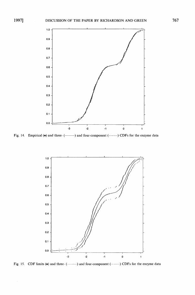
DISCUSSION O F THE PAPER BY RICHARDSON AND GREEN
-3 -2 -1 0 1
Fig. 14. (-) and three- (0 )Empirical and four-component (..........)CDFs for the enzyme data
-3 -2 1 0 1
Fig. 15. CDF limits (0 ) and three- (---) and four-component (..........) CDFs for the enzyme data

768 DISCUSSION OF THE PAPER BY RICHARDSON AND GREEN [No. 4,
and almost the same deviance. Fig. 15 gives a pointwise 95% confidence band for the true CDF based on the usual binomial interval, and the two fitted CDFs. Both fitted CDFs provide a close fit to the observed data.
In conclusion I have much pleasure in seconding the vote of thanks for a stimulating paper.
The vote of thanks was passed by acclamation.
D. R. Cox (University of Oxford): It is a pleasure to congratulate Dr Richardson and Professor Green on an impressive contribution. A possible further application is to problems in spectroscopy where a spectrum is to be decomposed into a mixture of an unknown number of Gaussian or Lorenzian components. Here the physical basis for the mixture model is reasonably firm. Even then I would be rather concerned at the possible overinterpretation that this, like other formally powerful methods, invites.
In Table 2 it is concluded from 82 irregularly distributed values well fitted by a mixture of four normals that the probability is 0.109 that eight normals really apply, etc. What does this really mean? This is partly but not entirely an issue of robustness of formulation of all parts of the model. If there were a physical theory suggesting a mixture to be appropriate, a minimal formulation leading to a confidence interval argument could in principle give only lower confidence limits for k. The authors' approach assumes more and therefore naturally gives stronger conclusions: but so much stronger?
The further assumptions are partly quantitative and partly structural. Seven tuning constants are needed to run the procedure, interpreted as constants in prior distributions. But these seven constants are calculated from the data. I conjecture that some of these can be regarded as roughly maximum likelihood estimates of parameters that are very poorly determined but also approximately orthogonal to the parameters of interest. From a Bayesian perspective they are aspects of a prior distribution, deter- mined from the data. There is nothing wrong in suitable cases in the choice of prior being influenced by the data, either for formal reasons as in the Bayesian treatment of the transformation problem (Box and Cox, 1964) or because seeing the data modifies the view taken of other information. This does, or should, affect the meaning of the answers. Put differently had these values been given by reliable substantive theory the answers would have been more meaningful. Probably, however, the more delicate assumptions are structural, especially perhaps the assumption that the component means are derived from normal order statistics, an assumption more critical the larger the value of k.
Would the authors agree with the following speculations?
(a) For models with small well fitting values of k the posterior intervals for component parameters have reasonable coverage properties.
(b) The posterior probabilities attached to the larger values of k are virtually substantively meaningless.
(c) More generally in similar applications conclusions that have no approximate confidence-interval- like interpretation will not make sense unless the prior distributions represent genuine new well- based information consistent with the data.
In many areas of statistics there are fairly strong protections partly formal and partly informal against overinterpretation. It may be that we are sometimes overcautious but some protection does seem necessary.
Matthew Stephens (University of Oxford): I restrict my comments on this stimulating paper to the problem of 'label switching' described in Section 4.3.1, conditioning on a fixed value of k. In some cases we have found that the 'obvious' relabellings of the sample points according to the order of the means or the order of the variances are not adequate and more sophisticated relabelling strategies are necessary. To illustrate this consider a Bayesian approach to estimation of parameters 17 = (w , p, u2) given a vague prior and 100 observations from the mixture density
where N (x; p, u2) denotes the probability density function of the normal distribution with mean p and variance u2. We use a Gibbs sampler to obtain a sample of size 10000 from the posterior distribution of the parameters given the true model.
Fig. 16 shows the sampled values of the means p = ( p l , p2, p3) and label switching is in evidence as P I , p2 and p3 are switched between the means near 0 (low variance), 5 (high variance) and 5 (low

19971 DISCUSSION O F THE PAPER BY RICHARDSON AND GREEN 769
Fig. 16. Means ( P I , p2, p3) sampled from the posterior by using the Gibbs sampler: (a) original sample; (b) relabelled sample
variance). Brief investigations confirmed that relabelling according to p l < p2 < p3 fails to separate the two components with mean 5 properly, whereas labelling according to < u: < u: fails to distinguish the two components with variance 1.
So by what criteria should we relabel our sample? We suggest that our relabelled sample should resemble a sample from a distribution in which the parameters of interest have unimodal marginal distributions. In this case we tried relabelling the sample so that it gives a good fit to some member of the natural conjugate family for the parameters
k
g(q; a, m, 1, u, n) = V(W; a) r]: ZG(cf; mi, It)N(pi; Ui, d l n i ) (14),=I
where V(w; a) is the density of the Dirichlet distribution with parameter a = (a,, . . ., ak) and ZG(a2; mi, 1,) is the density function of the inverse gamma distribution with parameters mi and 1,. This was achieved as follows.
Starting with the labelling given by the output of the Gibbs sampler iterate the following steps until we reach a relabelling which is unchanged by the iterations, or some upper limit on the number of iterations is reached:
(a) fit g(q; a, m, I, u, n) to the current labelled sample (by maximum likelihood say) to obtain an estimate (6, I,I, 6, A) for (a, m,l, u, n);
(b) for the ith sample point q n (I - 1, . . ., 10000), choose the relabelling u,(q(") which maximizes g{ai(q'"); 6,I,1, 6, A).
When applied to our example this method converges to a fixed labelling in 10 iterations. It seems from examination of the relabelled means (Fig. 16) that the method has been successful in selecting an appropriate relabelling, and this impression is reinforced by investigation of the relabelled mixture proportions and variances. By suitable choice of family (14) this method can be applied to mixtures of distributions other than normal.
Athanase Polymenis (University of Glasgow): I would like to mention a non-Bayesian method that is a modification of the minimum information ratio (MIR) method of Windham and Cutler (1992), and

DISCUSSION O F THE PAPER BY RICHARDSON AND GREEN
TABLE 4 Frequencies of selected values of k from 100 repetitions by using the basic MIR
method and the modijied MIR methodt
u Method Frequencies for the follo~ving values of k:
k = 2 k = 3 k = 4 k = 5
1.50
1.33
1
0.67
MIR Modified MIR
MIR Modified MIR
MIR Modified MIR
MIR Modified MIR
55 45 48 29 38
3 25 0
42 54 47 67 62 94 75 94
3 1 5 4 0 3 0 6
0 0 0 0 0 0 0 0
+The correct value is k = 3.
that I shall call the modified MIR method. If I is the Fisher information matrix for the mixture data and I, the Fisher information matrix for the associated complete data (i.e. where the subpopulation memberships are known), then the MIR is defined as the magnitude of the smallest eigenvalue of the information ratio matrix IC'.The MIR can also be expressed as 1 minus the EM convergence rate, and this result enables numerical calculation of the MIR values. Then, Windham and Cutler's method is to fit mixtures with various numbers of components and to choose the model for which the largest MIR is obtained.
The modification is based on a remark in Windham and Cutler (1992) that as soon as the model is overfitted the Fisher information matrix Ibecomes close to singular, so that the MIR drops suddenly to a value close to 0. Our method works as follows. Let k denote the number of components. Then, for each of the replicated samples we compare the ratio MIR(k + l)/MIR(k) with the corresponding ratios arising when we generate 99 bootstrap samples from the fitted k-component model; if this ratio is 'atypically large' then we increase k by 1 and repeat the procedure; otherwise we accept the current k as the solution.
Our simulation results have shown a distinct improvement in performance, relative to the basic MIR method. Here we briefly illustrate the modified MIR method on an artificial example from Windham and Cutler (1992), involving a mixture of k = 3 equally weighted bivariate normal components, with means at the vertices of an equilateral triangle and with spread measured by a parameter a; see Windham and Cutler (1992) for full details. We repeated their experiment, involving 100 replications and Table 4 compares the MIR and modified MIR in terms of how often a particular value of k was chosen; the modified MIR method is noticeably superior.
Walter R. Gilks (Medical Research Council Biostatistics Unit, Cambridge): The models and methods described in this paper are widely applicable. I myself struggled with similar models, in the pre- reversible-jump days of 1988. My task was to find clusters in patterns of reactivity of monoclonal antibodies. Typically, each data set contained around 60 antibodies, the observations on each antibody were 50 dimensional and around 20 antibody clusters were present. Each cluster represented an antigen (a protein) on the surface of white blood cells. My aim was to use Gibbs sampling to perform a Bayesian cluster analysis. Being stuck in a fixed dimensional world, my approach was to fix the number of clusters (groups) k, and to allow the Gibbs sampler to produce empty clusters. Thus the number of non-empty clusters was variable. This seemed fine in theory, but the empty clusters, having zero mass, would tend to fly wildly about the parameter space (when updating their location parameters p), giving little opportunity for wayward antibodies to hop aboard. Thus it was difficult for big clusters to break up or new ones to form, and mixing was generally poor. This was, I believe, the first published application of Markov chain Monte Carlo (MCMC) methods to mixture models (Gilks et al., 1989). Now, the methodology of the present paper provides just what I needed: the ability to design proposals to split, combine, create and kill clusters. Notwithstanding the rapid mixing of the samplers described in the present paper, I wonder whether this technology could produce rapid mixing in 50-dimensional prob- lems, without much slow and painful experimentation.

DISCUSSION OF THE PAPER BY RICHARDSON AND GREEN
TABLE 5 Posterior distribution for k for the galaxy data
An interesting extension to the models described in the present paper, which I had thought about in connection with the monoclonal antibody application, but was never able to implement, is to allow for a hierarchy of clusters: each cluster represents a cell surface antigen, and each subcluster represents an epitope (an outward projection) on the antigen. Some clusters will have subclusters, and others not. This would involve two sources of dimensional variability, and proposal distributions to split, combine, create and kill subclusters within clusters would be required.
I am not convinced by the authors' desire to produce a unique labelling of the groups. It is unnecessary for valid Bayesian inference concerning identifiable quantities; it worsens mixing in the MCMC algorithm; it is difficult to achieve in any meaningful way, especially in high dimensions, and it is therefore of dubious explanatory or predictive value. In the monoclonal antibody application, it is only the group members which lend meaning to the individual clusters.
Agostino Nobiie (University of Bristol): In a very stimulating paper, Richardson and Green have provided a full Bayesian analysis of finite mixtures, exploiting a new generation of Markov chain Monte Carlo (MCMC) samplers defined on the union of parameters-allocations subspaces with varying number of mixture components.
Before such new samplers, the obvious alternative consisted of evaluating the marginal density of the data under each mixture model pblk) , then using the prior on k and Bayes theorem to yield the posterior p(k1y). This was the approach taken in Nobile (1 994). The model considered there was slightly different from that entertained by Richardson and Green, with fixed P and a natural conjugate prior on the parameter 8: this permitted integrating w and 0 out of the problem and running the MCMC samplers (one for each value of k) on the space of allocations z. In Table 5 I report the posterior of k, with Monte Carlo standard errors SE, for the galaxy data set.
As noted above, the models do not match exactly; thus a and P were chosen to mimic some characteristics of Richardson and Green's prior. None-the-less the estimate of the posterior of k is similar to that reported in their Table I . Since they report no measure of the Monte Carlo variability of their estimates, I am led to believe that it is negligible. I consider this to be a major advantage of their procedure, over the method that I have illustrated above.
I would also like to comment briefly on the handling of the labelling problem. Richardson and Green clearly state that they restrict their attention to the case 'where we do not have (or want to use) strong prior information on the mixture parameters'. In this case requiring pl < . . . < pk is legitimate. In general, when prior information is available, its use may run contrary to the constraint. To exemplify, suppose that we know that if there are only two components one weight is much larger than the other. Then, use of this information requires us to assign a priori the components' labels and this assignment may be at odds with p1 < p2. I suggest including all prior information that might help to identify the model, while deferring to the post-processing stage the decision on whether and which constraints to impose. The necessary modification of the authors' sampler is straightforward.
I thoroughly enjoyed the paper, particularly the inventive displays of the complex posterior distribution employed by Richardson and Green, and I applaud their achievement.
Matthew Hodgson (University of Bristol): My comments concern the difficulties of meaningfully summarizing information in a posterior sample of functions. They originate from my experience in signal restoration in an ion channel, in which the signal is a binary step function. An initial estimate was obtained by thresholding the simulated posterior mean function at 50%, so that the estimated marginal modal value was taken at each point. This estimate performed well in misclassification terms but had an

772 DISCUSSION OF THE PAPER BY RICHARDSON AND GREEN [No. 4,
atypically low number of discontinuities (henceforth termed 'switches') compared with the posterior distribution of this number. Only switches with strong posterior support survived.
Consider more complicated estimates making better use of all the information contained in the sampler output. If we condition on a given number of switches s, perhaps the posterior median, we must then select the s switch times tl < t 2 < ... < t,. We might then think of choosing the mode of the joint density in s-dimensional space. Suppose, however, that there are S > s switch locations with non- negligible posterior support; then there may be of the order of
local maxima in the joint density! Choosing the highest peak becomes rather arbitrary if at all practicable. The marginal densities of the switch times will be multimodal, making a meaningful s- dimensional summary using them problematic.
I now describe an algorithm to construct a signal estimate having a given number of switches s. Choose cu E [O, 0.51, and assign one or other possible value to each point if and only if the estimated misclassification probability is not greater than a. This initial stage generates 'uncertainty intervals' containing unclassified points and also determines a certain minimal number of switches r. To make up the deficit of s - r switches we now decide how many extra switch pairs will be assigned to each uncertainty interval. We calculate the mean number of extra pairs in each interval by subsampling from the functions taking the 'correct' values at both ends, rank the intervals by this mean and assign an extra pair to the top (s - r)/2 intervals. Having decided the number of switches within each interval, we must suitably summarize their positions. For each interval, we use the mean positions conditional on the 'correct' function values at both ends and the 'correct' number of switches inside. This algorithm appears robust to the choice of cu below a 'critical value', typically around 0.3, beyond which it fails. Resulting estimates have only slightly greater misclassification rates than the original threshold estimate.
A. O'Hagan (University of Nottingham): This is a superb paper. To see the reversible jump Monte Carlo method flexing its muscles in this way is truly awe inspiring. My comments concern classification. Although the authors did not really talk about it, there has been much discussion about classification and the fact that a labelling problem is associated with it. An off-thecuff thought is that one way round this might be to look at pairs of observations, and simply to count how many times they are classified into the same mixture component. One obtains a nearness measure which could be used descriptively or could lead into clustering. I wonder whether this might be helpful.
Nicholas T. Longford (De Montfort University, Leicester): I would like to mention the EM algorithm, the principal tool for solving the mixture problem in a non-Bayesian formulation, and in particular its alternating expectation-conditional maximization (AECM) extension due to Meng and van Dyk (1997). In the AECM algorithm the unknown number of components can be accommodated integrally as a second layer of conditioning.
The full potential (and appeal) of Bayesian estimation would be realized if the process of defining the prior was more meaningful, e.g. based on (genuine) prior information. In the three examples, the definitions of prior have a somewhat ideological connotation rather than serving the originally intended purpose.
I would propose to side-step the issue of labelling by defining symmetric summaries, such as (multivariate) sample moments of up to the lowest order, from which the estimates can be recovered. These moments can be defined to promote their orthogonality and they may be useful in their own interpretive right.
A. P. Dawid (University College London): I would like to congratulate the authors on an impressive piece of work. I was concerned, though, about the labelling issue: this really only arises because we insist on trying to identify things which are essentially arbitrary.
As Professor Aitkin has pointed out, the model is essentially a random mixture model. For the normal case the 'parameter' is a mixing measure over (p, u) space. The authors take a discrete mixing measure, which can be represented by a finite number of points, with possibly different masses at each point. So, the prior distribution is really just a marked point process in (p, u) space. If there are many points in the process, perhaps variable in number, and we do not specify which one we are talking

19971 DISCUSSION O F THE PAPER BY RICHARDSON AND GREEN 773
about, it is pointless to ask where it is, or to try to express our uncertainty about its location: this is the labelling issue. But, if we think of the point process as the basic prior structure, we might think of other ways of describing it.
This approach also suggests that some of the established theory of point processes might be used as an alternative to the authors' prior structure. For example, perhaps Markov point processes might be realistic and lead to elegant analyses.
The following contributions were received in writing after the meeting.
A. C. Atkinson (London School of Economics and Political Science): I have three comments on this impressive display of computational skill in the pursuit of data analysis.
(a) The paper contains many examples of S-PLUS graphics. But, like Professor Aitkin, I find it difficult to judge goodness of fit from histograms. Professor Aitkin suggested plots of cumulative distribution functions. These also are not ideal, as they are bounded at 0 and 1. For problems with one component it is standard to use normal Q-Q-plots. Of course, such plots might be far from straight unless the correct plotting positions were calculated for the fitted k-component distribution. An alternative would be to simulate several samples (there is already much simulation in the paper) and to use a simulation envelope. Unlike the standard envelopes of Atkinson (1985), here the fitted distribution would have to be used in the simulation. Have the authors any experience of using plots to help to decide the number of components in their data?
(b) The measure of acidity in the lakes example takes values between about 4 and 7 and is pre- sumably the pH value. The authors suggest a log-transformation. Recently (Atkinson, 1995) I studied the transformation of multivariate data and found an example in which the log- transformation of pH was also indicated. Since pH is already the logarithm of the hydrogen ion concentration, I was rather uneasy. Do the authors have any suggestions for other models?
(c) I was surprised to learn after the talk that the numerical calculations were done in Fortran. It was in fact my experience with the calculations on multivariate transformations that led me to abandon Fortran. More recent work has been done in GAUSS. Do the authors have any recom- mendation?
Jo& M. Bernardo (Universitat de Valkncia): The authors are to be congratulated for providing another instance of the power and flexibility of the complete Bayesian analysis of complex models, which they make possible in a very important, difficult context, by using cutting edge Markov chain Monte Carlo techniques. There are, however, a couple of points that I would like to make.
Mixtures and model choice One of the frequent uses of mixtures is model choice. The univariate normal framework discussed in
the paper could presumably be used to obtain the authors' solution to stylized problems like 'testing' p = b , say, by using a mixture of N(xlb, no) and N(xIpi, u,),i = 1, . . ., k, where everything but b is unknown, and obtaining the posterior weight of N(xlpo, uo). I would like to see this run with some simulated data and compared with competing answers such as fractional Bayes factors (O'Hagan, 1995) or intrinsic Bayes factors (Berger and Pericchi, 1996). I suspect that the authors' solution may seriously depend on the prior chosen.
'Weak' prior information The 'default' prior which the authors suggest may be fine for a class of problems, but it may be
dangerous and misleading to suggest it as a general 'weak' information prior, for its consequences may crucially depend on the particular problem of inference that one chooses to study. For instance, I would expect that the proposed default prior would provide an unacceptable posterior for, say,
Again, this could easily be checked by running the algorithm with simulated data.
Really, both points are possible examples of a more general problem: in any Bayesian analysis, one is forced either to fine-tune a context-dependent subjective personal prior-a formidable task in complex problems, the result of which other colleagues might possibly disagree with-or to propose a 'default'

774 DISCUSSION O F THE PAPER BY RICHARDSON AND GREEN [No. 4,
prior which is bound to depend on the specific inference problem that is envisaged; an appropriate 'universal default' prior simply does not exist in any multiparameter model-see Bernardo (1997) for a recent discussion. The examples in the paper indicate that the default prior suggested for a mixture of normal models behaves sensibly in some classes of problems; it would be important for its users to know the conditions under which this might not be the case.
Julian Besag (University of Washington, Seattle): Green (1995) represents a breakthrough in the development of Markov chain Monte Carlo (MCMC) methodology and is already commanding widespread attention. The splendid paper by Sylvia Richardson and Peter Green demonstrates the power of the approach in just one of its many areas of application. Perhaps the main difficulty is in devising suitable moves and the authors negotiate this with considerable skill.
The following may possibly provide a slightly different perspective on reversible jumps. Consider a collection of target distributions pk(xk), indexed by k = 1, . . ., K. Here, according to context, k might identify the mixture composition (as in the present paper), the number of changepoints, the number of points in a spatial pattern, and so on. The pk can have different (fixed) dimensions and each may be composed of both discrete and continuous components. Now define a 'universal' target distribution,
where x = (xi, . . ., XK) and eachfi is a fixed distribution, perhaps independent uniform, with respect to the same measure as pi. Here, p(k) is a prior distribution or is implicit in the problem at hand, as would be usual for point processes. Simulation of p(x, k) can then be addressed in terms of a Metropolis- Hastings algorithm for a distribution of fixed dimension, in which moves from (x, k) to (x', kt) are proposed with xj =x, for I # k, k'. If k' # k, new xk and xk, are proposed, the former fromji and the latter usually closely related to xk. It is at this stage that one needs to ensure dimension matching and the existence of reverse moves but these arise in a natural fashion, together with the appropriate Jacobian. Note that the ji cancel out of the acceptance ratios and will be subject to eventual marginalization from the MCMC output, so they need never be sampled, nor even specified. Although k must be discrete, the existence of K is irrelevant. Whether or not this treatment is found helpful is perhaps mostly a matter of taste.
Multigrid MCMC sampling (e.g. Sokal(1989)) provides another special case of reversible jumps and was devised to combat severe multimodality in spatial systems in statistical physics. To give the flavour, in a more general setting, suppose one wishes to study a difficult distribution h(xo). Let xi, . . ., XK
denote 'coarsenings' of xo, which is now an additional component in x, and replace pk(xk) above by h(xo)pk(xklxo).Thepk are chosen so that the xk retain some of the characteristics of xo and can be used to generate viable but radically different proposals xb. There are some similarities to the split-combine moves in the paper. Possible applications include the construction of exact MCMC tests (Besag and Clifford, 1989, 1991) for hierarchical models in multidimensional contingency tables when standard algorithms are too sluggish.
S. P. Brooks (University of Bristol): I would first like to congratulate the authors on a stimulating and timely presentation of their work. It is comforting to see them evaluating the performance of their algorithm by examining its mixing properties. Their approach, which involves looking first at the mixing of the k-parameter and then at the mixing within k, certainly seems the most sensible approach. However, we might make the examination of the mixing of these algorithms more rigorous, improving on raw trace plots and plots of the ergodic average, by using any of the multitude of diagnostics proposed in the literature.
To assess the convergence of k is a very simple matter, since there are plenty of univariate diagnostic methods, such as those proposed by Gelman and Rubin (1992), Raftery and Lewis (1992), Geweke (1992) and Yu (1995). In fact, contrary to the authors' interpretation of Fig. 7, using any of these methods on the raw output (kindly provided by the authors) suggests that convergence of k has not yet been achieved, though this is disputed by the method of Heidelberger and Welch (1983). The problem of the assessment of convergence (mixing) within k is a little more complex, but since k is generally fairly small several multivariate methods might be appropriate, such as those proposed by Roberts (1992), Brooks et al. (1997), Brooks and Gelman (1996), Liu et al. (1993) and Ritter and Tanner (1992).
Using such methods, one might assess the convergence of k and then, once k appears to have reached

19971 DISCUSSION O F THE PAPER BY RICHARDSON AND GREEN 775
stationarity, look at convergence within each k. However, it is very likely that, even in a long run, some values of k will not be visited very often and thus the assessment of convergence within such k is almost impossible. Thus, a problem is associated with the selection of k-values to monitor.
Instead, we might not split the output in this way at all but apply the multivariate diagnostics to all parameters simultaneously. However, in the reversible jump Markov chain Monte Carlo case we do not know how many parameters there are, since k is allowed to vary. We could assume that all possible k- values have been seen in our single long run and assess convergence on that basis. But this is wrong: what about the k that we have not seen?
In fact, this is not a problem in the case presented in this paper, since the prior confines k to be less than k,,, = 30. Thus, we know exactly how many parameters there are. But what happens if we had a Poisson prior, for example? Clearly the assessment of convergence for this powerful technique is a serious issue; I would welcome the authors' views.
Simon Byers and Adrian Raftery (University of Washington, Seattle): We would like to thank Dr Richardson and Professor Green for their excellent exposition of the reversible jump Markov chain Monte Carlo (RJMCMC) method and of methodologies for exploring the rich output.
The RJMCMC method can be applied in two sometimes distinct contexts. In one, the underlying mixture (or other) model has a direct scientific motivation, and estimating the number of components and their means and variances is of primary interest. In the other context, the model dimension and parameters are not the quantities of direct interest. Green's (1995) image segmentation problem is of this type: there a synthetic Voronoi tiling was used to partition an image into two parts (feature and background).
We have been applying the RJMCMC method to a similar problem of the latter type: partitioning a spatial point process (not an image) into high density and low density regions. This arises, for example, in seismic fault location and mine-field detection (Byers and Raftery, 1996; Dasgupta and Raftery, 1995; Muise and Smith, 1992). We use a set of artificial points to generate a Voronoi tiling which partitions the region analysed; the number and position of the tiles is not directly relevant to the question of interest. In such cases, it might not be essential to allow the model dimension (here determined by the number of tiles) to vary; doing so will be justified only if it leads to a 'better' algorithm. When making this decision, the additional costs of RJMCMC relative to ordinary MCMC sampling should not be ignored (harder algebra; more complex programs; higher probability of errors; possibly lower accep- tance rates).
It is stated in the paper that RJMCMC followed by marginalization may provide better mixing than the fixed dimension algorithm. However, the very low acceptance rate of insertion and deletion of tiles in our example makes the RJMCMC algorithm somewhat slow. We have found that using a fixed but large number of tiles and simply moving tile generators by ordinary MCMC sampling gives much more frequent movement. Nevertheless, an occasional RJ move might be good to make a large jump. Perhaps a judicious combination of the two would be best, possibly changing dimension more often during the bum-in.
Gilles Celeux (Institut Nationale de Recherche en Informatique et Automatique, RhBnes-Alpes): Richardson and Green are among the few researchers who do not minimize the label switching problem in Bayesian analysis of mixtures. My comment concerns this problem. The mixture vector parameter (w, 8) is invariant under the permutations of the k labels of the components. As a consequence, the posterior distribution p(w, Bly) has (theoretically) k! intrinsic and symmetric modes. This posterior distribution is not interpretable in its own terms and there is a need to isolate one of its k! parts relative to a unique labelling. Label switching occurs when some labels of the mixture components permute.
A simple idea to deal with the labelling problem when running a Markov chain Monte Carlo (MCMC) algorithm is to force unique labelling by putting constraints to avoid label switching. Richardson and Green experiment with simple constraints. Mostly, they consider in a natural way that the means pk are in increasing order. They also consider other constraints such as ordering the variances &.
Forcing constraints for unique labelling when running an MCMC algorithm is not a good way to circumvent the problem. For instance, ordering the means pk can modify greatly the shape of the posterior distribution restricted to this unique labelling. The resulting posterior distribution can be expected to overweight the regions near the boundaries of the domain defined by the inequalities p1 < p2 < . . . < pk. This behaviour has been observed in unpublished numerical experiments, designed when preparing Celeux et al. (1996). As a consequence the posterior mean of 0 can be severely biased for

776 DISCUSSION OF THE PAPER BY RICHARDSON AND GREEN [NO.4,
poorly separated components. Moreover, choosing labelling constraints for multivariate mixtures is difficult.
A better way to deal with the label switching problem is to run MCMC algorithms without setting any constraint on the simulation parameters and then to permute the MCMC results by using data analysis tools. Stephens (1996) proposes an algorithm acting in such a way in a Bayesian spirit. A simpler way, with which we have experimented successfully, is to derive the labelling from the k! clusters obtained by the K-means algorithm performed on the normalized MCMC results.
But these solutions are difficult to incorporate in the reversible jump algorithm of Richardson and Green. In conclusion the label switching problem is a pitfall of Bayesian analysis of mixtures which has not yet been addressed satisfactorily and deserves more attention in the future.
R. C. H. Cheng and W. B. Liu (University of Kent, Canterbury): In the frequentist approach, if the model being fitted contains more components than that from which the data are actually drawn, then individual models are represented in the parameter space, not by a point, but by a subset (discussed for example by Feng and McCulloch (1996)). For instance if a two-component model
i: fittedJo data drawn from a single componentflx, Oo), then the estimation process can yield estimates 01 and 02 both close to 00 with & (unstably) between 0 and 1. A test is thus needed to check whether the components fitted are genuinely different; otherwise the estimated number of components needed can be erroneously high. Is there any reason why this same problem should not occur with the Bayesian approach (especially when there is great prior uncertainty about the number of components needed)? We are unclear how the authors' method addresses this issue. Thus for example in Table 1 for the enzyme data we suspect that the cases k = 4 where p(4) = 0.317 and k = 5 where p(5) = 0.206 are only obtained with two or more components very similar. They would then simply be alternative manifestations of the same case as k = 3 where p(3) = 0.290 and so should be subsumed into it and not treated separately. If this is the case, one would have p(k = 3) = 0.813, a much more conclusive inference, especially in the light of the practical application where the possibility that k = 3 is of especial interest.
Yung-Hsin Chien and Edward I. George (University of Texas, Austin): We would like to offer our congratulations to the authors for succeeding in providing a computable fully Bayesian approach for mixture modelling. This paper is a wonderful example of the huge potential for Bayesian modelling which continues to be unleashed by Markov chain Monte Carlo methods. Rather than criticize this excellent paper, we would like to discuss two possibilities for further development.
First, although we agree that fine-tuning of the proposal distribution may unduly increase compu- tational costs, we find it irresistible to suggest a refinement of the combine proposal. Currently, the combine proposal begins by randomly choosing a pair of adjacent components in the sense of having adjacent means. We wonder whether it might be more effective to define adjacency terms of a more comprehensive metric between distributions, perhaps based on an information distance. Of course, it would be necessary to use something inexpensive to compute. Intuitively, it would seem that adjacent components in this sense might be more natural candidates for combining and so would lead to higher acceptance rates. Furthermore, such a notion of adjacency would also be appropriate for higher dimensions and for different distributions. Finally, it might be advantageous to refine the combine step further by choosing a potential combination pair with probability inversely proportional to their dis- tance in terms of such a metric.
Second, although we agree that an advantage of the Bayesian approach is its sensitivity to the subtleties in the data, this sensitivity demands extra care in the formulation of the model. In particular, the meaning of k may depend heavily on the normality assumption for the components. For example, Fig. 2(a) for the enzyme data suggests that there are three components which are skewed rather than normal. If, in fact, this were the meaningful scientific answer to the problem, then the proposed method is simply using a mixture of normals to model different distributional forms, which would not be the real problem of interest. In Section 8.4, the authors discuss extending their approach to treat skewness as another random input. The key to evaluating the success of such an extension in such problems will hinge on whether it can avoid overfitting by putting larger probability on a smaller number of components.

19971 DISCUSSION OF THE PAPER BY RICHARDSON AND GREEN 777
Noel Cressie and Hsin-Cheng Huang (Iowa State University, Ames): This is a very nice paper that demonstrates how a fully Bayesian analysis can be carried out in mixture problems when the number of components is unknown. It shows us how to do what we hoped should have been possible, because, in principle, any statistical problem can be solved using a Bayesian approach.
Our discussion consists of two parts and is meant to expand the possible applications of the reversible jump Markov chain Monte Carlo (MCMC) method. First, in the paper, independence assumptions go quite deeply into the hierarchical model (see expressions (1H3)). Mixtures can occur in the analysis of spatial data, such as for remotely sensed data b(s l , s2): s1 = 1, . . ., M, s2 = 1, . . ., w.These might be reflectances that are noisy versions of the true intensity values {x(sl, s2)), discretized onto an M x N array of pixels. Regions of (approximately) constant x-values can be identified as objects and we assume x(sl, s2) E {pl,. . ., pk). Then the allocation variables z(.) are defined as z(sl, sZ) =j if x(sl, 2)= pj, j = 1, . . ., k. This is a mixture problem but in a setting where the distribution of the allocation variables z(.) probably should not be modelled as independent. A Markov random field model for z(.) (equivalently, x(.)) has been proposed by inter alia Derin and Elliot (1987), Pitas (1988), Short (1993) and Johnson (1994), although with k specified. The goal is to segment the scene into objects, i.e. to predict z(.). To obtain faster and better approximations to the maximum a posteriori estimator of z(.) when k is not specified in advance, Helterbrand and Cressie (1997) developed a multiresolution segmentation algorithm to find the posterior mode but they did not obtain the full posterior distributions. Do the authors think that their approach could be adapted to contextual segmentation (as described above) or, more generally, to (spatial) statistical problems where dependence is incorporated into the allocation variable? What problems might be encountered?
A second comment involves the application of the reversible jump MCMC method presented by Green (1995) to the problem of model choice. We have now seen how it can be implemented in mixture modelling. There is clearly potential for its application in other areas, such as order determination of autoregressive integrated moving average models in time series and wavelet representations of regression functions. Do the authors know of current work in these areas?
Marie-Anne Gruet (Institut Nationale de Recherche Agronomique, Jouy en Josas) and Christian P. Robert (Centre de Recherche en Economie et Statistique, MalakoQ: This paper illustrates the high potential of the reversible jump Monte Carlo technique in the Bayesian analysis of mixtures, but we would like to show that less symmetric alternatives are also available.
When the number of components k is unknown, the posterior distributionp(k, w, Olz, y) is defined on the space
2 = @ {k)x S k X @ k ,
k B Z(")
where S k is the simplex of w ~ - ' , Ok the k-component parameter set and z(,, the largest allocation. This distribution allows for a density with respect to the natural measure on 2 and thus for a regular Metropolis-Hastings implementation, by simulating k* from an instrumental distribution ?(k*Ik, z, y) and then (w*, 0*) from the true conditional p(w*, O*lk*, z, y), accepting the proposal of (k*, w*, 0*) with the usual probability ratio.
In the special case of normal mixtures, the instrumental distribution can be based on a random walk on k with jumps of f1. When the prior on k is a Poisson P(X)prior, the acceptance probability is then
This approach only cancels empty components, since k is constrained by k 2 z(,,, but it allows for faster moves between components since the new components are not restricted as in the split or merge move. Note also that the identifiability constraint can be transferred to the zs, in that the components are indexed as
This modification reduces the constraint on k and produces reasonable ranges of values for k, with smaller acceptance rates than in this paper (Gruet and Robert, 1997).

778 DISCUSSION OF THE PAPER BY RICHARDSON AND GREEN [NO.4,
Simon C. Heath (University of Washington, Seattle): I would like to present an application of the reversible jump Markov chain Monte Carlo method to genetic linkage analysis of extended pedigrees. Quantitative (continuous) traits are typically modelled as being controlled by either an infinite number of genes, each with infinitely small effect, or a small number of genes of larger effect. For the former approach, the genetic effect of each individual is normally distributed, and standard linear models techniques can be used. The latter approach, however, is more complicated because
(a) the genes controlling the trait must be modelled individually and (b) it is not known how many genes control the trait.
MCMC techniques have made it practical to model large numbers of genes individually, and now reversible jump MCMC methods allow inferences to be made about the number of genes controlling a trait.
One factor that complicates implementation of effective MCMC schemes for genetic linkage analysis is that the genotypes of pedigree members can show strong correlations both within and between loci. Simple genotype sampling schemes can exhibit poor mixing because of this; in particular, proposed moves which change the order or number of loci often have very low acceptance probabilities. Analytic integration of the genotypes for a given locus out of the acceptance ratio when proposing moving, adding or deleting that locus can result in higher acceptance probabilities and, therefore, a faster mixing sampler. A partial conditioning scheme (Besag et al., 1995) such as this requires the ability to sample the genotypes for a given locus, simultaneously for all pedigree members, from their full conditional distributions. Both the integration and sampling of genotypes rely on it being possible to 'peel' the pedigree (Elston and Stewart, 1971; Cannings et al., 1978) at the locus being changed; this is generally possible unless the pedigree is very complex (contains a large number of interconnected loops).
I have implemented a reversible jump MCMC sampler for genetic linkage analysis with large numbers of marker loci and extended pedigrees (Heath, 1997). Estimates of the number of loci affecting a trait, the probability of linkage of a trait locus to a chromosome and map position, size and allele frequency of trait loci can be easily obtained. The approach is more flexible than existing linkage analysis methods, and should increase our understanding of, and ability to model, quantitative traits.
C. lJennison (University of Bath): My comments concern the prior distribution for the parameters (p,, q)of a component of the mixture distribution. The authors appear keen to make this prior as 'non- informative' as possible. However, I believe such a goal will prove elusive in models with a variable number of dimensions as the choice of prior affects the posterior distribution of the number of dimensions-in contrast with the fixed dimensional case where just a few observations can yield a tight posterior distribution from a highly dispersed prior.
Consider the normal model with a fixed value of 7 = ([, K, a , P), so p, - N(c, K-I) and a;'- r ( a , p), j = I, 2, . . . . The posterior distribution of the number of mixture components, k, is pro- portional to the prior for k multiplied by the conditional density of the observed data given k,
Here r,,and 7ru2 denote prior densities for the pis and uis, p(z1k) is the conditional probability of the label vector z = (zl, . . ., z,,), given that there are k components, and 4 is the standard normal density; the p,s are not ordered in my notation. Rewriting pb lk) as
demonstrates the behaviour o f p b k ) as the priors x,, and r,: are made more disperse by decreasing K
and increasing p. For a labelling z which allocates rn > 1 observations to component j, the jth term in the product over j in expression (1 5) is of order K'I' as K + 0 and of order p-'" ' as + co;if sallocates no observations to component j, the term is 1 for any,x,, and x z . If one discounts the probability associated with empty components, as the prior on (pi, u;) grows more disperse, p b l k + I) decreases to

19971 DISCUSSION OF THE PAPER BY RICHARDSON AND GREEN 779
0 more rapidly than p(yJk)and the posterior distribution of k favours lower values of k . Thus, in the limit as K -+ 0 and p + m, the posterior probability of values of k > 1 is due solely to contributions from labellings that allocate all observations to just one mixture component.
Heuristically, a highly dispersed prior for (pj, a;?) allocates very little probability to values of (pj, uj) that are at all consistent with the data. The probability that several (p,, 4 ) s should all take values consistent with some of the data is extremely small and, hence, posterior probability concentrates on low values of k. This is seen in the dependence of the posterior distribution of k on P (Fig. 6(a)) and on K
(Section 5.1.2). The authors have treated K and /3 quite differently, introducing an extra model layer for ,B but
choosing a value for K directly, based on the range of the data. It would be interesting to see the effect of adding a similar extra layer for K: this might provide a convenient, automatic way of overcoming sensitivity to a prespecified value of n;however, I should hesitate to call such a prior 'non-informative'.
Andrew B. Lawson and Allan Clark (University of Abertay, Dundee): The idea of deconvolving cluster sums has been of interest in spatial statistics for some time. Often the intensity of a spatial point cluster process consists of a sum of contributions from r?, clusters {xi}, and this leads to a mixture problem with unknown ({xi}, r?,). Often these contributions depend on a cluster variance K , and hence, if K varies with cluster centre, on ki. The analysis of this problem was first suggested by Lawson (1993) and inde- pendently by Baddeley and van Lieshout (1993). An example of a fully converged sampler applied to an epidemiological problem where K is a function of a spatial Gaussian field appears in Lawson (1995). This development of cluster samplers was based on theoretical convergence results for reversible jump samplers (birth-death shifting transitions) by Geyer and Mnrller (1994).
Several issues arise from work on spatial cluster processes which are very relevant to the current DaDer. r - ~ r - -
First, it is often found that the likelihood in cluster or mixture problems is very spiky (i.e. large areas of low likelihood occur mixed with small areas of high likelihood). This can lead to multiple-response problems (commonly found in object recognition in imaging). To combat this, an inhibition prior distribution (e.g. a Strauss distribution) is often assumed for {xi} (or in the authors' case {pi}). An alternative is to smooth the likelihood by penalization.
Second, the variable z, which the authors use for component membership, can be regarded as an auxiliary variable, as it is not directly required in the reconstruction of the components. This dichotomy was alluded to by Binder (1978), and the inclusion or otherwise of z leads to the specification of a complete or incomplete problem. Do the authors have any insight into the effect of exclusion of step (c) from their algorithm?
Third, the use of a shifting transition in addition to a birth-death transition could have been used by the authors in step (f) but has not been included. This could facilitate exploration of the posterior surface. This addition has been used in clustering examples. Have the authors considered this addition?
Finally, spatial clustering mixture problems usually assume that wi = Ilk, Vi, and hence there is no requirement to include weight generation steps in such problems. In the algorithm described by the authors, the weights {wi} are included. However, in the suggested algorithmic steps the authors appear to update the weights twice: first in step (a and then recomputed in the birthdeath step. Should not the 1 . .birthkleath step generate new p: and up jointly with the w,?
Geoff McLachlan and David Peel (University of Queensland, Brisbane): It is of interest to compare the results of this Bayesian approach applied to the three real data sets with those working in a frequentist framework. Consequently, we fitted kcomponent univariate normal mixture models with unrestricted component variances by maximum likelihood via the EM algorithm of Dempster et al. (1977); see also McLachlan and Krishnan (1997). There can be complications for normal components with unrestricted variances, arising from the fact that the likelihood becomes infinite with fitted components corresponding to a single observation. This is a potential problem in particular for the galaxy data set which contains some clusters of relatively few points. One way to avoid this is to impose a lower bound on the ratios of the fitted component variances. The results reported below for this data set are those obtained without any restrictions on the ratios of the variances.
The choice of the number of components k was made in terms of the increase in the log-likelihood as k was increased sequentially from k = 1. As is well known, regularity conditions do not hold for the usual asymptotic null distribution of the likelihood ratio X to be valid. Here the P-value was assessed by using the resampling approach as in McLachlan (1987).

DISCUSSION OF THE PAPER BY RICHARDSON AND GREEN P o . 4, TABLE 6
Assessed P-values obtained for the three data sets
Data set P-values for k versus k + 1 for the following no. of components k:
I 2 3 4 5 6
Acidity 0.01 0.08 0.44 - - -Enzyme 0.01 0.02 0.06 0.39 - -Galaxy 0.01 0.01 0.01 0.04 0.02 0.22
In Table 6, we report these assessed P-values for the three real data sets. It can be seen that in two cases in Table 6 the assessed P-value lies between 5% and 10%. Performing further bootstrap replications in these cases did not clarify the situation. Also, these assessed P-values should not be interpreted too finely, as it is the bootstrap rather than the actual P-value that is being assessed in these cases since the null value of k is greater than 1.
On the basis of these P-values interpreted rigidly at the 5% level of significance, k would be chosen to be 2, 3 and 6, for the acidity, enzyme and galaxy data sets respectively. If the significance level were increased to lo%, it would result in k being chosen equal to 3,4 and 6 for the acidity, enzyme and galaxy data sets respectively. This is in general agreement with the results obtained here in a Bayesian framework for k, except in part for the acidity data set. For this set, the Bayesian approach provides essentially equal support for k = 2-6, whereas, according to the P-values assessed by resampling, one would not go beyond k = 3 components.
K. Mengersen and A. George (Queensland University of Technology, Brisbane): Through their analysis of mixture distributions with an unknown number of components, Richardson and Green have demonstrated some of the versatility and power of Green's reversible jump sampler. Our experience with this approach is in its application to the ordering of gene markers on a chromosome and positioning of a quantitative trait locus (QTL) relative to the markers. These problems are characterized by complex likelihoods represented as mixtures with a large number of parameters, entire classes of missing information (e.g. half-sib designs) and a large model space related to the number and position of the markers and QTLs.
Despite this complexity, the implementation of Green's algorithm was refreshingly simple. A countable set of move types, based on genetic principles, was sufficient to characterize the model space independently of the number of gene markers. Moreover, the nature of the algorithm permitted a ready generalization of the problem in several directions and much less preanalysis of the model space than an alternative model selection strategy (Carlin and Chib, 1995) with which we have also had experience.
The assessment of convergence of Markov chain Monte Carlo algorithms remains an area of intense research. For Richardson and Green's methodology, as in all such stochastic search algorithms for model determination, two issues arise. First, there is the question of whether the chains can (and do) adequately traverse the model space, especially when a successful move requires (chance) generation of a favourable combination of many parameters with complex relationships. In simulation this is easy to check, but in practice it is more difficult than Richardson and Green intimate. Second, there is the problem of assessing the overall convergence of the realized chains, especially those traversing the model space. Existing accessible diagnostics have mainly a univariate focus, give at best pessimistic estimates of run lengths and often target a specific facet of convergence. The use of a combination of such diagnostics does not obviate the need for 'holistic' tests applicable to the model selection situation. In all, although we are delighted with our experience of the reversible jump methodology, the convergence issue urges a critical evaluation of the results of any such analysis.
Anne Philippe (UniversitC de Rouen, Mont-Saint-Aignan): This paper presents an interesting im- plementation of a Markov chain Monte Carlo (MCMC) algorithm for the complex mixture model. In spite of the apparent convergence of their method, a discussion of the assessment of convergence for this form of MCMC algorithm would be most welcome. In particular, could the authors relate their assessment to fixed k settings to that proposed below in the set-up of an exponential mixture (as discussed by Robert)?

19971 DISCUSSION O F T H E PAPER BY RICHARDSON A N D GREEN 78 1
The Monte Carlo method can lead to different estimators of the integral TKf(h). When f is a density on a set of dimension 1, an alternative to the empirical average is to consider the Riemann sum estimator (see Philippe (1996) or Robert (1995)). For a sample (XI, . . . .x,,) fromf, this estimator is given by
where x(l) ,< .. . < x(,) are the order statistics associated with the sample. In many MCMC set-ups, the density f is unknown, as in the particular case of the exponential
mixture, and the estimator (16) is not available. However, we can generalize equation (16) by using the Rao-Blackwell estimator of the marginal density in Gibbs sampling settings (see Philippe (1996)). The resulting estimator is
where .rr is the conditional distribution of the parameter of interest x l E R, given the other parameters x2, . . . . xp. This estimator can be implemented for the estimation of the parametersp and X of the two- components exponential mixture p Exp(X) + (1 -p) Exp(Xr) (see Fig. 17). Moreover, when we consider h(x) = 1, this alternative approach provides a convergence criterion. Indeed, the estimator (17) clearly converges to the known value 1. Therefore, we can monitor the convergence of this estimator for the marginal densities of the different parameters of the mixture (see Fig. 17 for p and A).
Fig. 17. (a) Empirical average (----) and Rao-Blackwellized Riemann sums (..........), (b) convergence control and (c) histogram and empirical versus true cumulative density function for a sample of 100 observations from 0.5 Exp(5) + 0.5 Exp(O.5)

782 DISCUSSION O F THE PAPER BY RICHARDSON AND GREEN [No. 4,
Kathryn Roeder and Larry Wasserman (Carnegie Mellon University, Pittsburgh): We congratulate Dr Richardson and Professor Green for their very interesting contribution to the Bayesian analysis of mixtures. Mixtures are tailor made for Markov chain Monte Carlo (MCMC) methods and the authors have developed a particularly ingenious version for this problem. We find ourselves in agreement with most of what the authors say. There are a few points that we would like to raise.
First, we wonder whether the reversible jump technology-which perhaps deserves a more fash- ionable name like 'transdimensional MCMC'-is not just a little too clever. Separate runs for different values of k seem simpler even if we must then estimate the normalizing constant, a challenging but not impossible task. DiCiccio et a[. (1997) have reviewed the many methods for doing this. Have the authors made any direct comparisons of their method with a 'separate runs' analysis?
Second, we agree that a prior with little influence is desirable. If we understand correctly, the prior on the means has variance depending on the range of the data. But such a prior is asymptotically improper. This is undesirable because dimension estimation, or Bayes factor calculations, are ill defined for improper priors. Would it not be better to use a prior that is asymptotically pro er? A different prior 4' and r/ tthat we find useful is this: the means are N(0, r2), the variances are ~ ~ ~is ~ ~ 1 ~ : ; the overall location 0 is given a flat prior and the overall scale A is given the prior T(A) a 1/A; finally, the hyperparameter v is set equal to 1 (Roeder and Wasserman, 1997). This model involves no data- dependent priors and seems to be insensitive to the choice of v. Also, the complete conditionals are simple distributions.
Finally, the Dirichlet process mixture (DPM) approach is more closely related to the model in this paper than one might think. Instead of a finite Dirichlet prior on wl, . . ., wk the DPM takes wl = zl, w2 = z2(1- zl), wj = z3(l - zl)(l - z2),. . . where zj -- beta(1, a),j = 1, 2, . . . . Another difference between the models is that k is assumed to be infinite for the DPM and hence there is no need to do any dimension estimation. The prior on a takes the place of a prior on k. Notice that we have not even mentioned the Dirichlet process, which is really a red herring, in this description. The DPM merely induces a slightly different prior on the weights.
Peter Schlattmann and Dankmar Btibning (Free University, Berlin): The paper by Sylvia Richardson and Peter Green provides new valuable insights into the analysis of mixtures. The Bayesian approach by means of reversible jump Markov chain Monte Carlo methods opens the opportunity not only to have posterior distributions on all the parameters of a finite mixture of normal densities,
for samples X I , . . ., x,, but also on the number of components k. (Here P denotes the distribution giving weight pj to a parameter combination p, and uj.) One additional nice aspect of the approach proposed can be seen in the fact that it circumvents the well-known problem of non-existence (Lindsay, 1995) of maximum likelihood estimates (MLEs) if different variances are allowed in every sub- population.
It should be pointed out that in the approach proposed many parameters (of prior distributions) must be estimated or prespecified. Also, the computational burden increases and to what extent data reduc- tion can be achieved needs to be evaluated.
We would like to emphasize that traditional maximum likelihood approaches also allow an investigation of the variability of the number of components k. There is a long tradition for obtaining MLEs for mixtures with unknown k which exploit the geometry of the mixture problem, usually called the nonparametric mixture model approach (Laird, 1978; Lindsay, 1983; Bohning, 1985; Bohning et al., 1992). In this approach also the number of components is estimated such that the discrete distribution on the parameter space which maximizes the likelihood is found. This approach works best for the one-parameter exponential family whereas for the normal distribution a boundary condition for the common variance parameter is necessary.
Reliable computational algorithms (Bohning, 1995) exist and are implemented in the software packages C.A.MAN (Bohning et al., 1992) and DismapWin (Schlattmann et al., 1996).
The distribution of the number of components k may be obtained by applying the mixture algorithm B times to bootstrap samples (xy , . . ., x,*) obtained from the original sample with replacement.
As an example (to demonstrate the alternative way of illustrating the variability in the estimate l)we

19971 DISCUSSION OF THE PAPER BY RICHARDSON AND GREEN 783
provide the bootstrap distribution of for the acidity data obtained after B =5000 replications:
Here the nonparametric mixture approach would indicate heterogeneity consisting of at least two components. Applying the likelihood ratio test of Ho: k = 2 against H I : k = 3 leads to rejection of HI with a value of -2 log X = 5.542, which is non-significant at the 5% level according to the simulation studies of Thode et al. (1988) with their results transferred to our situation.
D. M. Titterington (University of Glasgow): The reversible jump idea promoted in this paper offers an interesting new Bayesian approach to the analysis of mixture data, and the applications to real data are appealing. I think that major challenges now are to implement the method in the context of more complicated mixtures, such as the multivariate cases considered in Section 8.1, and to assess the method against possible underlying questions of interest.
For instance, if the mixture model is to be taken seriously rather than just as a version of a latent structure model, so that the number of components, k, has some 'physical' meaning, then how is the marginal distribution fork to be used, especially if it is important to infer a 'point estimate' for k, even if that goes against the Bayesian spirit expressed for instance in Table 2? This question, of course, has generated all the non-Bayesian work caused by the non-regularity of the likelihood ratio statistic. It would be interesting to investigate the performance of the posterior mode of k in this respect, but an alternative candidate might be the smallest k for which the posterior probability becomes 'appreciably positive'. Of course, this characteristic would have to be properly defined, no doubt through the 'deviances' mentioned at the end of Section 4.1, but it would for instance lead to choosing k = 3 for the enzyme data, rather than the modal value of k = 4. Such a choice of k would correspond to the smallest k that is meaningfully supported by the data. In a somewhat similar vein Mr Polymenis's contribution, in the context of a different, frequentist cjterion, shows that it is more effective to select k not by optimizing that criterion but by choosing k - 1, where k is the smallest k for which the mixture seems clearly too rich.
If, however, the mixture model is only to be regarded as a flexible density estimator, I wonder whether this particular Bayesian approach will catch on in competition with, say, kernel-based methods, even though the mixture formula is more parsimonious. Of relevance here might be the work of Priebe (1994) and, here again, the practicability of the method in higher dimensions will be important.
Howell Tong (University of Kent, Canterbury): It is known (e.g. exercise 29 on p. 212 of Tong (1990)) that the following threshold autoregressive model admits, under very general conditions, a stationary marginal distribution which is the mixture of distributions:
where the a s are real constants and (€1) is a sequence of independent, identically distributed random variables each with zero mean and with E , being independent of X,, s < t . For example, if 6, has a zero- mean normal distribution then the stationary marginal for X, is a mixture of k normal distributions with different locations. If we want greater generality in having a mixture of k distributions which are different in form, location and scale, we only need to allow the white noise terms (namely the €-terms) in the different regimes to be different. It is a challenging problem to determine, from the dependent data say ( X I ,Xz, . . ., XN), simultaneously the order d, which happens to be equal to the delay parameter in this set-up, and the number of regimes, namely k. I would welcome comments from the authors on whether and how they could extend their Bayesian approach to cover this problem.
Mike West (Duke University, Durham): This mixture context provides a nice framework, indeed a showcase, for the implementation of Bayesian analysis using reversible jump Markov chain Monte Carlo (MCMC) methods. My only complaint is that the restriction to univariate deconvolution or

784 DISCUSSION OF THE PAPER BY RICHARDSON AND GREEN [No. 4,
density estimation problems seems unambitious, as the approach applies readily to multivariate mixtures and more challenging, though accessible, applied problems.
I have a few specific comments and connections to draw.
(a) On identification and parametric constraints, West (1997) describes how the posterior symmetries resulting from the inherent 'labelling' feature can be exploited in assessing the convergence of MCMC analyses. Though presented in a specific class of structured mixture models, the ideas there apply widely.
(b) On classification and discrimination, Lavine and West (1992) presented the first 'fully Bayesian' (Gibbs-sampling-based) approach with an illuminating two-dimensional normal mixture example that may interest readers in this area.
(c) The use of Dirichlet mixtures, with implicit 'Poisson-like' priors over numbers of components, is more geared towards density estimation and related objectives than deconvolution or parameter estimation; here the number of components is treated simply as a nuisance parameter to be averaged away. One attraction of these models has been the ease of extension to multivariate problems (West et al., 1994; Miiller et al., 1996).
(d) In problems where mixture deconvolution is really of primary focus, I am sceptical of the benefits of adopting reversible jump methods compared with the usual 'nested models' approach based on fixing an upper bound and assigning a prior on the number up to that bound. In a neuro- physiological application (West, 1997), for example, highly structured mixture models and priors arise naturally from the physical and experimental context. Here the number of components is a function of the underlying number of synaptic transmission sites at a neural junction under investigation. We have found it very fruitful to explore inferences based on fixed numbers of sites, sequentially increasing the number and assessing changes in resulting inferences after repeat analysis. This approach is coupled with a 'screening' analysis that adopts an upper bound on the number of sites, and hence the number of components, and then performs MCMC analysis to assess the number of sites in this more usual 'nested modelling' framework. Standard Gibbs sampling applies within this nested model framework: easily implemented and effective. It would be of interest to compare this with the alternative MCMC methods of the authors, with a focus on the overheads incurred in developing and tuning the required 'jumping rules'.
The authors replied later, in writing, as follows.
We are delighted that our paper has provoked a wide-ranging and lively discussion, and we thank all the discussants for their contributions and their interest in the topic.
Complexity Some discussants (Aitkin, Cox, Schlattmann and Bohning) have categorized our approach as
overcomplex. We contest this and claim that the key components of hierarchical Bayesian modelling,
(a) the complete data structure, including the allocation indicators used by both Bayesian and EM- type procedures,
(b) the treatment of k as random, allowing us to explore the mixture fully with a single analysis rather than carry out separate analyses which need to be put together coherently-a difficult task in maximum likelihood (ML) analyses, and finally
(c) a prior model for the component parameters, which can express weak informativeness flexibly, and circumvents the potential problems associated with boundary values, referred to by Aitkin, McLachlan and Peel, and Schlattmann and Bohning,
capture and clarify the essential elements of finite mixture estimation. Equation (4) is thus a coherent way to structure the ingredients underlying any mixture analysis.
Cox emphasizes the need for seven tuning constants in our approach. However, the hyperparameters A, 6, (,n, a,g and h should not be grouped together: a one-parameter family of priors for k indexed by X was introduced for generality, but it is not used, and similarly 6 is fixed at 1, providing the uniform prior on the weights that would be used in most analyses. The other five hyperparameters are used in the prior model for the means and variances. We have chosen not to link these quantities. The dependence of some of these on the interval of variation of the data is natural on grounds of symmetry and scale invariance; this should not be regarded as data-based estimation of the prior. There remain four

19971 DISCUSSION O F THE PAPER BY RICHARDSON AND GREEN 785
numerical constants in our default hyperparameter settings: K = 1/R2,CY = 2, g = 0 .2 and h = R2.Here we have used plausible choices, supported by deliberate assumption and/or by sensitivity studies.
Interpretation and labelling Many comments have been concerned with the problem of labelling and interpretation of the
components (the connection between labelling and mixing of the Markov chain Monte Carlo (MCMC) sampler will be discussed along with other MCMC issues). As pointed out in our paper, mixture estimation is camed out with various aims. At one end of the spectrum are situations where there is firm scientific evidence for the existence of finite mixtures, e.g. genetic polymorphism, or in spectroscopy, as cited by Cox. In this case, identifying and labelling the components is meaningful and can be achieved by post-processing the output and labelling to seek unimodal density estimates for the component parameters. This can be performed by a variety of methods, either by imposing simple constraints as illustrated in our paper, or by using clustering-like procedures along the lines suggested by Gilks and Celeux, and implemented and demonstrated by Stephens. O'Hagan's pairwise comparison is another possibility. The success of such an exercise will depend on the separation of the components. If there is strong overlap, the labelling cannot be unambiguous. To clarify Celeux's comments, we stress that the use of ordering in our sampler is consistent with our target density and does not create any bias, but that in running simulation studies one should be aware that not applying the same labelling constraints on the output and on the truth would bias the results. In a multidimensional set-up, we agree with Gilks that it is the clusters which give meaning to the components.
At the other extreme, finite mixtures are used as semiparametric density estimates, as emphasized by Aitkin, and may even be regarded as an approximation of continuous mixtures. We agree with Aitkin that, in this case, no interpretation should be given to the components and that only summaries which are invariant to the labelling, like density estimates or the symmetric summaries of Longford, should be produced. We agree that density estimation is also important but do not want to be drawn into qualifying the relative importance of the two contexts. Between these two extremes, there are many cases to which we could refer to as exploring heterogeneity (the lake acidity and the galaxy data can be placed in this category), where heterogeneity can be hypothesized but latent indicators have not yet been identified. Post-processing the output is then a means to bring out a range of (possibly competing) representations supported by the data, which can help to give clues towards understanding the source of heterogeneity.
We cannot agree with Robert that the meaning of individual components is 'vacuous', but the meaning does rely entirely on the choice of labelling constraint.
Departing from full Bayesian paradigm The contrast between the Bayesian and other approaches to mixture analysis has focused most
strongly on inference about k. The standard paradigm can be caricatured as choosing the smallest k such that the model fits. This principle derives partly from parsimony, and partly from necessity: it is difficult to fit the parameters of any more components than that, or to avoid reliance on hypothesis testing as a tool for the choice of k.
In the Bayesian approach, parsimony can be specified more directly, through prior modelling. Parsimony is not a feature of the weakly informative prior, with default parameter values, that we have used to present our results, but parsimonious priors may be handled readily with our methods (see the next section).
Our calculations produce a good approximation to the joint posterior distribution of all unknowns; what is done with this is limited more by imagination than by rules of Bayesian analysis, and it is certainly not obligatory simply to quotep(k1y) and to abandon any attempt at model interpretation or selection, if the context demands. Titterington's suggestions of choosing the mode of k or the smallest k for which there is 'some support' and Robert's suggestion are examples; other possibilities worth exploring could be the monitoring of changes in the predictive densities or quantifying the overlaps in the posterior distributions of the deviances.
These last two suggestions could be broadly interpreted as attempting in a Bayesian context to quantify 'overfitting', which in a classical framework could be detected by looking for singularity of the Fisher information matrix, as proposed by Polymenis with his modified minimum information ratio method.
In this spirit, like Cox we would refrain from reliance on values of p(k1y) for large k. The right-hand tail is especially sensitive to the arbitrariness in the prior on k that we used, which we recall was adopted

786 DISCUSSION OF THE PAPER BY RICHARDSON AND GREEN [No. 4,
only for computational convenience. In the absence of 'reliable substantive theory', inference about the right-hand tail is problematic; a fully convincing weakly informative approach perhaps needs more structure not less!
We happily acknowledge the important contribution of ML-based methods to mixture analysis, whether fitted through the EM algorithm (McLachlan and Peel), alternating expectation~onditional maximization (AECM) (Longford) or from the angle of nonparametric maximum likelihood (NPML) estimation (Aitkin, Schlattmann and Bohning) discussed comprehensively by Lindsay (1995). We find the comparisons interesting and we thank the discussants who took the trouble to report them. Overall, the conclusions of McLachlan and Peel on the number of components for our three data sets are in agreement with our discussion above on how we would exploit the full joint posterior distribution with respect to model choice. For the acidity data, the conclusions of Schlattmann and Bohning, and McLachlan and Peel differ somewhat from ours and would be more compatible with an analysis using a prior with more spaced-out means (see the next section). We did not allow for the stratification in our analysis of the acidity data because it was not used in Crawford (1994) and we wanted to be able to compare our conclusions with hers. Looking at Table 3 reported by Aitkin on NPML analysis of the enzyme data (after logarithmic transformation), we notice that, for k = 3, NPML fails really to find a third component, the reported weight being only around 0.01. In contrast, running our model on the same logarithmically transformed data, we find a mode for p(k1y) at k = 3 (with a posterior probability of 0.51) and posterior expectations for the means and weights of the three components equal respectively to (0.23, - 1.67, - 2.80) and (0.38, 0.55, 0.07). Thus we agree with Aitkin only for the means of the first two components but not the weights, and in our case we find a genuine third component. Furthermore, the uncertainty in these estimates can be assessed, whereas this is more difficult for ML analyses, as admitted by Aitkin.
Prior structures and non-informativeness Prior structure of the mixture parameters is clearly a central issue and is referred to by many
discussants; it is an issue which cannot be dissociated from the objective of the mixture analysis. We shall comment in turn on alternative prior structures and more parsimonious inference and then on the question of non-informativeness in mixture analysis.
We agree with Longford that scientific evidence for the existence of the mixture should be incorporated into the prior model as well as possible; an interesting example is given by West. Let us say that the prior structure that we have proposed is best adapted to the aim described above as exploring heterogeneity. The priors proposed by Roeder and Wasserman could be also adapted to that purpose; the essential difference is the link that they postulate between the means and the variances. It will certainly be interesting to carry out some comparisons. Separation of the components has been queried by Cheng and Liu. As increasing numbers of components are fitted-which can be done in our framework without encountering singularity problems- the separation will clearly decrease, but not to the extent that they surmise. To give an example, for the enzyme data, the posterior mean of the minimum separation between the component means is 0.19 and 0.11 for k = 4 and k = 5 respectively. Nevertheless, if parsimony is a concern, there may be interest in our experiments with a different prior structure for the means, which jointly defines the {p,;j = 1, 2, . . ., k ] as the s , 2.9, . . ., ks order statistics from a sample of size ks + s - 1 from N(( , K - ' ) , thus encouraging separation through the choice of s, to a degree which can be calibrated apriori. This is akin to an inhibition prior referred to by Lawson and Clark, or a spatial point process prior as suggested by Dawid. The results are not unexpected: both the posterior mean and the variance of k are reduced as s is increased from 1 to 3. For example, we see a clear posterior mode at k = 3 for the enzyme data, and posterior probabilities for k = 2 increasing from 0.20 to 0.36 when s is varied from 2 to 3 for the acidity data. This leads to a tighter posterior distribution for k and more parsimonious model choice, which could answer some of the concerns expressed on this point by Aitkin, Besag, Cox and Titterington.
We find ourselves in agreement with Bernardo's insightful exposition of the impossibility of defining a 'universal default prior'. We certainly do not regard our default setting as universal and took care to assess it with a sensitivity study, but we have not examined it in other inferential contexts such as those that he mentions. Note that the range we use is supposed to correspond to a notional interval of variation, independent of sample size (in the reported analyses the observed range was used only for convenience), thus not creating the problems of asymptotic impropriety pointed out by Roeder and Wasserman. Their interesting alternative choice, which links the mean and variance, requires only one tuning constant. This linking amounts to making hidden assumptions about quantities that are

19971 DISCUSSION O F THE PAPER BY RICHARDSON AND GREEN 787
analogous to our hyperparameters. We would be interested to see studies on sensitivity to this choice, and to perform some comparisons.
Jennison provides a careful analysis, that essentially supports our contention that with independent priors any attempt to approach non-informativeness too closely is doomed, although a detail we would quibble with is his choice of fixing a while letting P +co.A possible means for countering some of the degeneracy that he demonstrates would be to modify the model to condition the allocations to ensure non-empty components. The line that he suggests, of introducing an extra model layer for K, analogous to that for p, was incorporated in the first version of our paper but omitted both to save space and because it did not seem to solve the problems uncovered in Section 5.1.2.
Finally, we want to comment on the separate issue of prior models and density estimation. We agree with West that other prior models, such as those based on Dirichlet processes, are attractive. We have started experimenting with them within our reversible jump structure. We are not convinced by Robert, that a sensible procedure is first to select a value of k, & say, and then to do density estimation conditional on &. It is computationally more cumbersome than the density estimate that we produce, it is not fully Bayesian and its justification on the ground of parsimony do not seem to us appropriate in the context of density estimation.
Model extensions Many discussants have suggested extensions of the mixture model. One line of extension relates to
implementing our approach for other families of densities while keeping the same graphical model structure.
We agree with West and Titterington that generalizing our approach to multivariate mixtures is important and challenging, and might call for additional sets of moves, possibly along the lines suggested by Chien and George. One extension that we have implemented is the generalization to a skew normal family by using the transformation y ~+(exp(py) - l]/p, with a common skewness parameter p for all components, which creates a wide variety of distributional shapes. This parameter requires another move type, a Metropolis step. It is then possible to investigate the joint posterior of k and p. For the enzyme data this posterior gives a strong indication of high skewness, though not as strong as a logarithmic transformation, and favours fewer components, as surmised by Chien and George: the mode forp(k1y) is achieved at k = 2 (with a posterior probability of 0.39). Interestingly, having the extra flexibility of a family of skewed transformations gives more support for two components than log- transforming directly (see the discussion above).
Other extensions of the mixture model, in particular to spatial or image applications, will require the lifting of some of the conditional independence assumptions, as noted by Cressie and Huang. Spatial structure can be introduced, for example, by modelling the weights or the joint distribution of the allocations as a spatial process. When k is unknown, added difficulties arise in connection with the need to evaluate normalizing constants.
Summarizing posterior distributions The choice of scales and functions for plotting to compare data with fitted distributions is partly a
matter of taste: densities and histograms are most familiar, but we could have used cumulative distributions or Q-Q-plots, as advocated by Aitkin and Atkinson respectively. Either could have been displayed in analogues of Figs 2 and 3(b) (although we strongly prefer to stick to densities for parameter posteriors such as in Figs 4, 5 and 9(b)). Atkinson suggests showing simulation envelopes in these comparisons. This is very natural in the Bayesian context and does not involve any additional simulation. Pointwise credibility bounds for cumulative distribution functions, or the quantiles used in Q-Q-plots, are readily computed directly from the MCMC samples, and with not much extra effort (see Besag et al. (1995)) simultaneous bounds are also available. All these tools are of course principally focused on the nonparametric distribution estimation facet of mixture modelling, rather than on the heterogeneity itself.
Hodgson usefully highlights and addresses some of the difficulties in presenting posterior information about functions, especially those with non-linear parameterizations (as in his example and ours). It would be interesting to try to adapt his procedure to mixture estimation when, as sometimes happens, the interest is primarily in the number of modes, rather than the number of components: Bayesian density estimates with any prescribed number of modes could thereby be produced.
Reversible jump technicalities Several discussants comment or make suggestions on the moves used in our sampler. As we stated, we

788 DISCUSSION OF THE PAPER BY RICHARDSON A N D GREEN [No. 4,
experimented to only a limited extent-tuning was minimal-and do not claim our choice to be optimal; it would be interesting to study these questions further, but we are somewhat sceptical that there will be great advantages gained from doing so for univariate mixture models.
Alternative moves are proposed by Chien and George, combining (and splitting) on the basis of a different measure of adjacency, which we like; the last part of this idea would be expensive, however- reversibility must not be sacrificed, so that choosing a pair to combine with unequal probabilities means that, when splitting, all components must be split on a test basis, simply to compute these probabilities. Lawson and Clark ask about moves that update w, p and a at the same time as splitting and combining; this is of course possible, though it adds complication. Note that moves (a) and (b) do directly follow (e) and (f) in sequence. Their idea of omitting (c) could be taken two ways; literally, it is possible, and it may at least be sensible, to do (c) rather rarely as it is somewhat expensive and typically makes only modest changes. But their phraseology suggests something else, namely integrating out the allocations z from the model altogether, which would totally change the algorithm, probably for the worse. We would be interested in comparing our mixing performance for the same model parameterization with that of the alternative sampler, conditioning on the allocations, proposed by Gruet and Robert. Byers and Raftery surprise us with their suggestion of attempting a dimension change only rarely, on grounds of expense. Three of their four components of expense (algebra, complexity and errors) are not mitigated by their suggestion. Running time is a factor in determining the balance of investment of effort on different move types, but the optimal balance is a subtle and complex matter that we do not believe is yet understood.
We are grateful to Besag for making the connection with multigrid samplers; usually these operate on a systematic schedule over dimensions, but one can certainly envisage random sweep versions. In the case of the stochastically blocked samplers of Kandel et al. (1989), the analogy with the present methods is perhaps even closer. Besag's alternative representation of variable dimension MCMC simulation, placing all xk in one big product space, is interesting: it provides an explicit common dominating measure for all variables. We are not clear that it necessarily simplifies the formulation of the acceptance ratio, unless one goes the extra step of integrating aN the innovation variables u of Section 3.1 into the frame as well.
The role of labelling of components in the sampler needs to be clarified. Contrary to the suggestion of Gilks, Celeux, Robert and Gruet, using adjacency (in terms of means) in the splitkcombine move actually improves performance; the modified program we have that ignores adjacency, mentioned by Nobile (and coded by him!) gives slightly inferior mixing. We emphasize that, except for this move, the only point in our entire methodology where labelling is used is in the output analysis, when we wish to make marginal inference about components, as in Section 4.3.
We regret omitting reference to Gilks (1989) and were intrigued by his picture of empty components roaming unfettered in outer space; his intuition here seems close to ours in adopting the birth-and-death move to discipline empty components when the prior is particularly weak.
West points out that, in a nested model context, dimension changing is possible with standard MCMC techniques. However, there may be a loss of performance relative to our method: as a partial test of his suggestion, we ran our sampler on the galaxy data with k fixed at 10, suppressing moves (e) and (f), and found greatly inferior mixing for the number of non-empty components.
Comparisons with separate runs on each model Distinct from the possibility of departing from the full Bayesian paradigm in making inference about
k is that of achieving that paradigm by means of separate MCMC runs within each value of k, seaming these together to form the full joint posterior. In answer to Roeder and Wasserman, no, we have not tried this, but Agostino Nobile has, and we refer to his contribution for some of the details. Our conclusion is to stick to our approach, at least for mixtures and other problems where the models being entertained interleave in a similar fashion: note the side-benefit described in Section 6.2.2. We would certainly like to use some of the powerful tools presented in DiCiccio et al. (1997) where the rival models are less closely related and construction of dimension-changing jumps might be problematical. On terminology, PJG prefers to retain the 'reversible jump' tag rather than anything flashier: we think that it is pedagogically useful to regard this as just Metropolis-Hastings sampling in a general state space and see all the moves as of the same general character-in contrast with the 'jumpdiffusion' dichotomy of Grenander and Miller (1994).
Diagnostics An assessment of convergence in variable dimension problems is difficult; the best approach may be

19971 DISCUSSION OF THE PAPER BY RICHARDSON AND GREEN 789
to focus on monitoring statistics which have meaning independent of dimension, e.g. functionals of predictive densities. Invariances can sometimes be exploited, as suggested by West; Philippe also has an interesting proposal. An assessment of convergence simultaneously for all parameters is especially challenging and will doubtless be the focus of future work.
We thank Brooks for carrying out diagnostics for k, spumng us to take a closer look at convergence. For brevity, we only comment on diagnostics performed on two runs of 500000 sweeps, started either a t k = 1 or at k = 30, for the galaxy and acidity data sets. We agree with Brooks that diagnostics like those of Gelman and Rubin, and Geweke give some indication that convergence may not be reached in 200000 sweeps, in particular for the galaxy data. These diagnostics improve when the number of sweeps is increased to 500000. Even longer runs are needed according to the method of Raftery and Lewis. The sequence of values of k is highly autocorrelated, as expected; for some runs small haphazard shifts of level are detected, suggesting some room for improved mixing. Nevertheless we stress that the sub- stantive conclusions on p(k1y) are essentially unchanged after the initial 200000 sweeps.
In his interpretation of the allocation plotted in his Fig. 13(c), as compared with those of Fig. 12(c), Robert seems to confuse posterior uncertainty (indicated by the variation in grey levels vertically) with slow convergence (highlighted by instability in this variation, and sometimes the presence of irregular stripes). For our own model and method, applied to the galaxy data without bum-in, the corresponding plot in Fig. 18 shows uniform texture, suggesting satisfactory mixing and stability.
Computing environment Atkinson asks about our computing environment. This was a combination of Fortran and S-PLUS.
The modem dialect of Fortran that we used seemed admirable for the numerical calculations involved in the sampling; the only special feature of the programming lay in the use of lists to organize the components of the mixture (linked in numerical order of (p,)), and the observations allocated to each component. All the looping involved was straightforward with use of 'while' loops, and would have
40
data rank
Fig. 18. Allocation map for our analys~s of the galaxy data, conditioning on k = 6, based on a run of length of 100000with no burn-in

790 DISCUSSION O F T H E PAPER BY RICHARDSON A N D GREEN [No. 4,
been very slow in S-PLUS. Selected results of each run of the sampler were dumped out into a large collection of files with structured file names. We then used a suite of S-PLUS functions, each reading one or more of these files and producing a plot or some other output analysis. This proved a powerful and flexible combination for our research: in a production environment, we might have coupled the Fortran and S-PLUS codes more closely by using dynamic loading and fewer files. Finally, the codes were written carefully to ensure that exactly the same numerical results are obtained on both an IBM workstation in Paris and a Sun workstation in Bristol, even replicating the random number streams.
Other reversible jump applications Heath, and Mengersen and George describe genetic applications of reversible jump samplers. This is
an important area where these techniques are promising and are currently generating much interest. One of us (SR) has also been collaborating with Duncan Thomas on applications of this methodology to the problem of multipoint linkage analysis with an unknown number of trait loci (Thomas et al., 1997) in which a dimension jump is used to add and delete loci and their associated parameters.
Tong, and Cressie and Huang refer to reversible jump in the context of model choice for time series. We note that a fully Bayesian version of Tong's threshold autoregressive model would treat the parameters r, also as unknowns, and that there is some similarity to the changepoint problems discussed by Green (1995); the time series dependence does not greatly affect the set-up, but the variable delay parameter is a novelty. Model choice for autoregressive moving average models using a reversible jump has been recently considered by Barbieri and O'Hagan (personal communication). Cressie and Huang ask about applications to wavelets: the nearest work that we are aware of is by Miiller and Vidakovic (1995).
Spatial point processes are evidently productive territory for reversible jump applications: we were interested to hear of the work of Byers and Raftery, and Lawson and Clark, on modelling heterogeneity and clusterine res~ectivelv. ... .
Gilks refers to the need in hierarchical clustering for more than one varying dimension component; another rather general context where this is needed is the approach to Bayesian analysis of variance based on mixtures that is being explored at Bristol, involving nested and, especially, crossed par- titioning.
To conclude this section and our rejoinder, we were fascinated by all the on-going research reported by discussants, and we hope that they will keep us informed of future developments.
REFERENCES IN THE DISCUSSION
Aitkin, M. (1996) A general maximum likelihood analysis of overdispersion in generalized linear models. Statist. Comput., 6, 251-262.
(1997) A general maximum likelihood analysis of variance components in generalized linear models. To be published.
Atkinson, A. C. (1985) Plots, Transformations, and Regression. Oxford: Oxford University Press. (1995) Multivariate transformations, regression diagnostics and seemingly unrelated regression. In MODA
4-Advances in Model-oriented Data Analysis (eds C. P. Kitsos and W. G . Miiller), pp. 181-192. Heidelberg: Physica.
Baddeley, A. and van Lieshout, M . (1993) Stochastic geometry models in high-level vision. In Statistics and Images (ed. K. Mardia), pp. 233-258. Abingdon: Carfax.
Berger, J. 0 . and Pericchi, L. R. (1996) The intrinsic Bayes factor for model selection and prediction. J. Am. Statist. Ass., 91, 109-122.
Bernardo, J. M. (1997) Noninformative priors do not exist: a discussion. J. Statist. Planng Inf., to be published. Besag, J. and Clifford, P. (1989) Generalized Monte Carlo significance tests. Biometrika, 76, 633-642.
(1991) Sequential Monte Carlo p-values. Biometrika, 78, 301-304. Besag, J., Green, P., Higdon, D . and Mengersen, K. (1995) Bayesian computation and stochastic systems (with
discussion). Statist. Sci., 10, 3 4 6 . Binder, D . (1978) Bayesian cluster analysis. Biometrika, 65, 31-38. Bohning, D . (1985) Numerical estimation of a probability measure. J. Statist. Planng In$, 11 , 57-69.
(1995) A review of reliable maximum likelihood algorithms for semiparametric mixture models. J. Statist. Planng Inf., 47, 5-28.
Bohning, D., Schlattmann, P. and Lindsay, B. G . (1992) C.A.MAN-computer assisted analysis of mixtures: statistical algorithms. Biometries, 48, 283-303.
Box, G . E. P. and Cox, D. R. (1964) An analysis of transformations (with discussion). J.R. Statist. Soc. B, 26,211-252. Brooks, S. P., Dellaportas, P. and Roberts, G. 0 . (1997) A total variation method for diagnosing convergence of
MCMC algorithms. J. Comput. Graph. Statist., to be published.
19971 DISCUSSION OF THE PAPER BY RICHARDSON AND GREEN 791
Brooks, S. P. and Gelman, A. (1996) Alternative methods for monitoring convergence of iterative sin~ulations. Technical Report. University of Cambridge, Cambridge.
Byers, S. D. and Raftery, A. E. (1996) Nearest neighbor clutter removal for estimating features in spatial point processes. Technical Report 305. Department of Statistics, University of Washington, Seattle (available at http://www.stat.washington.edu/tech.reports/tr305.ps).
Cannings, C., Thompson, E. A. and Skolnick, M. H . (1978) Probability functions on complex pedigrees. Adv. Appl. Probab., 10, 26-61.
Carlin, B. P. and Chib, S. (1995) Bayesian model choice via Markov chain Monte Carlo methods. J. R. Statist. Sac. B, 57, 473484.
Celeux, G., Chauveau, D. and Diebolt, J. (1996) Stochastic versions of the EM algorithm: an experimental study in the mixture case. J. Statist. Computn Simuln, 55, 287-314.
Crawford, S. L. (1994) An application of the Laplace method to finite mixture distributions. J. Am. Statist. Ass., 89, 259-267.
Dasgupta, A. and Raftery, A. E. (1995) Detecting features in spatial point processes with clutter via model based clustering. Technical Report 295. Department of Statistics, University of Washington, Seattle (available at http://www.stat.washington.edu/tech.reports/tr295.ps).
Dempster, A. P., Laird, N. M. and Rubin, D. B. (1977) Maximum likelihood from incomplete data via the EM algorithm (with discussion). J. R. Statist. Soc. B, 39, 1-38.
Derin, H . and Elliot, H. (1987) Modeling and segmentation of noisy and textured images using Gibbs random fields. IEEE Trans. Paftn Anal. Mach. Intell., 9, 39-55.
DiCiccio, T., Kass, R., Raftery, A. and Wasserman, L. (1997) Computing Bayes factors by combining simulation and asymptotic approximations. J. Am. Statist. Ass., to be published.
Elston, R. C. and Stewart, J. (1971) A general model for the genetic analysis of pedigree data. Hum. Hered., 21, 523-542.
Feng, Z. D. and McCulloch, C. E. (1996) Using bootstrap likelihood ratios in finite mixture models. J. R. Statist. Soc. B, 58, 609417.
Gelman, A. and Rubin, D. (1992) Inference from iterative simulation using multiple sequences. Statist. Sci., 7,457-511.
Geweke, J. (1992) Evaluating the accuracy of sampling-based approaches to the calculation of posterior moments. In Bayesian Statistics 4 (eds J. M. Bernardo, A. F. M. Smith, A. P. Dawid and J. 0 . Berger), pp. 169-193. New York: Oxford University Press.
Geyer, C. and M ~ l l e r , J. (1994) Simulation procedures and likelihood inference for spatial point processes. Scand J. Statist., 21, 84-88.
Gilks, W. R., Oldfield, L. and Rutherford, A. (1989) Statistical analysis. In Leucocyte Typing IV (eds W. Knapp, B. Dorken, W. R. Gilks, S. F. Schlossman, L. Boumsell, J. M. Harlan, T. Kishimoto, C. Morimoto, J. Ritz, S. Shaw, R. Silverstein, T. Springer, T. F. Tedder and R. F. Todd), pp. 6 1 2 . Oxford: Oxford University Press.
Green, P. J. (1995) Reversible jump Markov chain Monte Carlo computation and Bayesian model determination. Biometrika, 82, 71 1-732.
Grenander, U. and Miller, M. I. (1994) Representations of knowledge in complex systems (with discussion). J. R. Statist. Soc. B, 56, 549403.
Gruet, M. A. and Robert, C. P. (1997) Estimating the number of components in a normal mixture. Technical Report. Universitk de Rouen, Mont-Saint-Aignan.
Heath, S. C. (1997) Markov chain Monte Carlo segregation and linkage analysis for oligogenic models. Am. J. Hum. Genet., to be published.
Heidelberg, P. and Welch, P. D. (1983) Simulation run length control in the presence of an initial transient. Ops Res., 31, 1109-1 144.
Helterbrand, J. D. and Cressie, N. (1997) Object identification using Markov random field segmentation models at multiple resolutions of a rectangular lattice. Lect. Notes Statist., 122, 159-1 73.
Izenman, A. J. and Sommer, C. J. (1988) Philatelic mixtures and multimodal densities. J. Am. Statist. Ass., 83, 941-953.
Johnson, V. (1994) A model for segmentation and analysis of noisy images. J. Am. Statist. Ass., 89, 23G241. Kandel, D., Romany, E. and Brandt, A. (1989) Simulations without critical slowing down: Ising and three-state Potts
models. Phys. Rev. B, 40, 33G344. Laird, N. (1978) Nonparametric maximum likelihood estimation of a mixing distribution. J. Am. Statist. Ass., 73,
805-811. Lavine, M. and West, M. (1992) A Bayesian method for classification and discrimination. Can. J. Statist., 20, 451-
461. Lawson, A. (1993) Discussion on the meeting on The Gibbs sampler and other Markov chain Monte Carlo methods.
J. R. Statist. Soc. B, 55, 6 1 4 2 . (1995) Markov chain monte carlo methods for putative pollution source problems in environmental epi-
demiology. Statist. Med., 14, 2473-2486. Lindsay, B. G . (1983) The geometry of mixture likelihoods: I, A general theory. Ann. Statist., 11, 8 6 9 4 .

792 DISCUSSION O F T H E PAPER BY RICHARDSON A N D GREEN [No. 4,
(1995) Mixture models: theory, geometry, and applications. In NSF-CBMS Regional Conference Series in Probability and Statistics, vol. 5. Hayward: Institute of Mathematical Statistics.
Liu, C., Liu, J, and Rubin, D. B. (1993) A control variable for assessment of the convergence of the Gibbs sampler. Proc. Statist. Comput. Sect. Am. Statist. Ass., 74-78.
McLachlan, G . J. (1987) On bootstrapping the likelihood ratio test statistics for the number of components in a normal mixture. Appl. Statist., 36, 318-324.
McLachlan, G . J. and Krishnan, T. (1997) The EM Algorithm and Extensions. New York: Wiley. Meng, X.-L. and van Dyk, D. (1997) The EM algorithm -an old folk-song sung to a fast new tune (with discussion).
J . R . Statist. Soc. B, 59, 51 1-567. Mengersen, K. and Robert, C. (1996) Testing for mixtures: a Bayesian entropy approach. In Bayesian Statistics 5
(eds J . 0 . Berger, J. M. Bernardo, A. P. Dawid, D. V. Lindley and A. F. M. Smith). Oxford: Oxford University Press. To be published.
Muise. R. and Smith. C. (1992) Nonoarametric minefield detection and localization. Technical Reoort CSS-TM-591- 91. ~ a v a lSurface h a i f a r e cent&, Panama City.
Miiller, P., Erkanli, A. and West, M. (1996) Bayesian curve fitting using multivariate normal mixtures. Biometrika, 83, 67-79.
Miiller, P. and Vidakovic, B. (1995) Bayesian inference with wavelets: density estimation. Discussion Paper 95-33. Institute of Statistics and Decision Sciences, Duke University, Durham.
Nobile, A. (1994) Bayesian analysis of finite mixture distributions. PhD Thesis. Carnegie Mellon University, Pittsburgh.
O'Hagan, A. (1995) Fractional Bayes factors for model comparison (with discussion). J. R. Statist. Soc. B, 57, 99-138.
Philippe, A. (1996) Connections between Monte Carlo and numerical methods. TEST, 5, 218-223. Pitas, I. (1988) Markovian image models for image labeling and edge detection. Signal Process., 15, 365-374. Priebe, C. E. (1994) Adaptive mixtures. J. Am. Statist. Ass., 89, 796-806. Raftery, A. E. and Lewis, S. M. (1992) How many iterations in the Gibbs Sampler? In Bayesian Statistics 4 (eds J . M.
Bernardo, A. F. M. Smith, A. P. Dawid and J . 0 . Berger). Oxford: Oxford University Press. Ritter, C. and Tanner, M. A. (1992) Facilitating the Gibbs sampler: the Gibbs stopper and the griddy-Gibbs sampler.
J . Am. Statist. Ass., 87, 861-868. Robert, C. P. (1995) Convergence control methods of Markov chain Monte Carlo algorithms. Statist. Sci., 10, 231-
253. Robert, C. P., Chauveau, D., Diebolt, J., Gruet, M. A,, Guihenneuc, C., Lassere, V., Muri, F., Philippe, A. and
Richardson, S. (1997) Control of MCMC algorithms via finite state space Markov chains. Lect. Notes Statist., to be published.
Robert, C. P. and Mengersen K . L. (1995) Reparameterisation in mixture models and their bearing on the Gibbs sampler. Working Paper 9547. Centre de Recherche en Economie et Statistique, Malakoff.
Robert, C. P. and Titterington, M. (1996) Resampling schemes for hidden Markov models and their application for maximum likelihood estimation. Submitted to Statist. Comput.
Roberts, G. 0. (1992) Convergence diagnostics of the Gibbs sampler. In Bayesian Statistics 4 (eds J . M. Bernardo, A. F. M. Smith, A. P. Dawid and J. 0 . Berger). Oxford: Oxford University Press.
Roeder, K. and Wasserman, L. (1997) Practical Bayesian density estimation using mixtures of normals. J. Am. Statist. Ass., to be published.
Schlattmann, P., Dietz, E. and Bohning, D. (1996) Covariate adjusted mixture models and disease mapping with the program DismapWin. Statist. Med., 15, 919-929.
Short, T . (1993) An algorithm for the detection and measurement of rail surface defects. J.Am. Statist. Ass., 88,436-440.
Sokal, A. D. (1989) Monte Carlo methods in statistical mechanics: foundations and new algorithms. Cours de Troisiime Cycle de la Physique en Suisse Romande. Lausanne.
Stephens, M. (1996) Dealing with the multimodal distributions of mixture model parameters. Preprint. Thode, H. C. , Finch, S. J. and Mendell, N. R. (1988) Simulated percentage points for the null distribution of the
likelihood ratio test for a mixture of two normals. Biometries, 44, 1195-1201. Thomas, D. C., Richardson, S., Gauderman, J. and Pitkaniemi, J. (1997) A Bayesian approach to multipoint
mapping in nuclear families. Genet. Epidem., 14, in the press. Tong, H. (1990) Nonlinear Time Series: a Dynamical System Approach. Oxford: Oxford University Press. West, M. (1997) Hierarchical mixture models in neurological transmission analysis. J.Am. Statist. Ass., 92, 587-606. West, M., Miiller, P. and Escobar, D. (1994) Hierarchical priors and mixture models with application in regression
and density estimation. In Aspects of Uncertainty: a Tribute to D. V. Lindley (eds A. F . M. Smith and P. R. Freeman). Chichester: Wiley.
Windham, M. P. and Cutler, A. (1992) Information ratios for validating mixture analyses. J. Am. Statist. Ass., 87, 1188-1 192.
Yu, B. (1995) Discussion to Besag et al. (1995) Statist. Sci., 10, 3 4 6 .