on an efficient solution strategy of newton type for ... · 1 universität dortmund on an efficient...
TRANSCRIPT
1
Universität Dortmund
On an efficient solution strategy of Newton type forimplicit finite element schemes based on algebraic flux correction
Matthias [email protected]
Institute of Applied Mathematics (LS III)University of Dortmund, Germany
ICFD Conference on Numerical Methods for Fluid Dynamics26–29 March 2007, University of Reading, UK
Overview Algebraic flux correction Nonlinear solution algorithm Numerical examples Outlook Conclusions and Outlook References Appendix
2
Universität Dortmund
Overview
Algebraic flux correction
MotivationDesign principlesFlux limiting
Nonlinear solution algorithm
Choice of preconditionersConstruction of JacobiansNumerical examples
Outlook
Application to compressible flowsGrid adaptivity
Conclusions
Overview Algebraic flux correction Nonlinear solution algorithm Numerical examples Outlook Conclusions and Outlook References Appendix

3
Universität Dortmund
Motivation
Scalar transport equation
∂u
∂t+∇ · (vu) = 0
High-order methods: wiggles
0 0.1 0.2 0.3 0.4 0.5 0.6 0.7 0.8 0.9 1
0
0.2
0.4
0.6
0.8
1
Standard Galerkin FEM
Mcdu
dt+ Ku = 0
Low-order methods: smearing
0 0.1 0.2 0.3 0.4 0.5 0.6 0.7 0.8 0.9 1
0
0.2
0.4
0.6
0.8
1
Remedy: nonlinear combination of high- and low-order discretizations.
Overview Algebraic flux correction Nonlinear solution algorithm Numerical examples Outlook Conclusions and Outlook References Appendix

4
Universität Dortmund
Algebraic flux correction, Kuz05a
High-order scheme Mcdudt + Ku = 0 K = kij,∃kij > 0, j 6= i
Apply artificial diffusion D = dij, dij = −maxkij , 0, kji = dji
Low-order scheme Mldudt + Lu = 0 L = K + D, lij ≤ 0,∀j 6= i
Decompose the residual difference into internodal fluxes
rHi − rL
i =∑j 6=i
fij , fij =[−mij
ddt + dij
](uj − ui ) = −fji
Nonlinear high-resolution scheme containing limited antidiffusion
Mldudt + Lu = f , fi =
∑j 6=i
αij fij , 0 ≤ αij ≤ 1
Overview Algebraic flux correction Nonlinear solution algorithm Numerical examples Outlook Conclusions and Outlook References Appendix

5
Universität Dortmund
Flux limiting
Nonlinear high-resolution scheme (lumped-mass version)
Mldu
dt+ Lu = f , fi =
∑j 6=i
αij fij , fij = dij(uj − ui ) = −fji
αij ≡ 0 ⇒ f = 0 ⇒ Mldudt + Lu = 0 low-order scheme
αij ≡ 1 ⇒ f = Du ⇒ Mldudt + Ku = 0 high-order scheme
Goal: Determine αij as close to 1 as possible such that
(Lu − f )i =∑j 6=i
qij(uj − ui ), qij ≤ 0 ∀j 6= i
Overview Algebraic flux correction Nonlinear solution algorithm Numerical examples Outlook Conclusions and Outlook References Appendix

6
Universität Dortmund
Nonlinear solution algorithm
Nonlinear algebraic system for 0 < θ ≤ 1 N(u) := Lu − f
Mlun+1 − un
∆t+ θN(un+1) + (1− θ)N(un) = 0
Fixed-point iteration u(0) := un
u(m+1) = u(m) − C−1F (u(m)), m = 0, 1, . . .
until ‖F (u(m+1))‖ ≤ tol or ‖F (u(m+1))‖ ≤ tol‖F (un)‖.
Practical implementation
C∆u(m+1) = F (u(m))
u(m+1) = u(m) −∆u(m+1)
m = 0, 1, . . .
u(0) = un
Overview Algebraic flux correction Nonlinear solution algorithm Numerical examples Outlook Conclusions and Outlook References Appendix

6
Universität Dortmund
Nonlinear solution algorithm
Nonlinear algebraic system for 0 < θ ≤ 1 N(u) := Lu − f
F (un+1) := Mlun+1 − un
∆t+ θN(un+1) + (1− θ)N(un) = 0
Fixed-point iteration u(0) := un
u(m+1) = u(m) − C−1F (u(m)), m = 0, 1, . . .
until ‖F (u(m+1))‖ ≤ tol or ‖F (u(m+1))‖ ≤ tol‖F (un)‖.
Practical implementation
C∆u(m+1) = F (u(m))
u(m+1) = u(m) −∆u(m+1)
m = 0, 1, . . .
u(0) = un
Overview Algebraic flux correction Nonlinear solution algorithm Numerical examples Outlook Conclusions and Outlook References Appendix

7
Universität Dortmund
Choice of preconditioner
Linearized system C∆u(m+1) = F (u(m))
Diagonal mass matrix C = Ml/∆t
cheap, but only usable for very small time steps
Low-order operator C = Ml/∆t + θ L
fixed-point defect correction scheme may converge slowlyno update needed if the velocity field remains unchanged
Jacobian operator C = Ml/∆t + θ ∂N(u)∂u
nonlinear operator N(u) is constructed discretelyflux limiter may not be globally differentiable
Idea: approximate by divided differences and see what happens
Overview Algebraic flux correction Nonlinear solution algorithm Numerical examples Outlook Conclusions and Outlook References Appendix
8
Universität Dortmund
Jacobian matrix, Moe07a
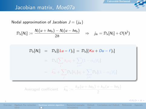
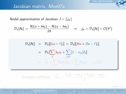
Nodal approximation of Jacobian J = jik
Dk [Ni ] :=Ni (u + hek)− Ni (u − hek)
2h⇒ jik = Dk [Ni ] +O(h2)
Dk [Ni ] = Dk [(Lu − f )i ] = Dk [(Ku + Du − f )i ]
= Dk [∑
j
kijuj +∑j 6=i
(1− αij)fij ]
= kik +∑
j
Dk [kij ]uj +∑j 6=i
Dk [(1− αij)fij ]
Averaged coefficient kik :=kik(u + hek) + kik(u − hek)
2
Overview Algebraic flux correction Nonlinear solution algorithm Numerical examples Outlook Conclusions and Outlook References Appendix
8
Universität Dortmund
Jacobian matrix, Moe07a
Nodal approximation of Jacobian J = jik
Dk [Ni ] :=Ni (u + hek)− Ni (u − hek)
2h⇒ jik = Dk [Ni ] +O(h2)
Dk [Ni ] = Dk [(Lu − f )i ] = Dk [(Ku + Du − f )i ]
= Dk [∑
j
kijuj +∑j 6=i
(1− αij)fij ]
= kik +∑
j
Dk [kij ]uj +∑j 6=i
Dk [(1− αij)fij ]
Averaged coefficient kik :=kik(u + hek) + kik(u − hek)
2
Overview Algebraic flux correction Nonlinear solution algorithm Numerical examples Outlook Conclusions and Outlook References Appendix

9
Universität Dortmund
Sparsity pattern, Moe07a
Jacobian coefficients jik = kik +∑
jDk [kij ]uj +∑
j 6=iDk [(1− αij)fij ]
There exists an edge ij iff the FE basisfunctions have overlapping supports
G := 〈K 〉 gii = 1, gij = 1 ⇔ ∃ij
Structure of the Jacobian Z := 〈J〉zkk 6= 0, zik 6= 0 ⇔ ∃ik
zjk 6= 0 ⇔ ∃ik ∧ ∃ij
Remarks
Same structure is used for edge-oriented stabilization techniques
Sparsity pattern can be generated by multiplication: Z = G 2
Overview Algebraic flux correction Nonlinear solution algorithm Numerical examples Outlook Conclusions and Outlook References Appendix

9
Universität Dortmund
Sparsity pattern, Moe07a
Jacobian coefficients jik = kik +∑
jDk [kij ]uj +∑
j 6=iDk [(1− αij)fij ]
There exists an edge ij iff the FE basisfunctions have overlapping supports
G := 〈K 〉 gii = 1, gij = 1 ⇔ ∃ij
Structure of the Jacobian Z := 〈J〉zkk 6= 0, zik 6= 0 ⇔ ∃ik
zjk 6= 0 ⇔ ∃ik ∧ ∃ij
u hek k±
Remarks
Same structure is used for edge-oriented stabilization techniques
Sparsity pattern can be generated by multiplication: Z = G 2
Overview Algebraic flux correction Nonlinear solution algorithm Numerical examples Outlook Conclusions and Outlook References Appendix

9
Universität Dortmund
Sparsity pattern, Moe07a
Jacobian coefficients jik = kik +∑
jDk [kij ]uj +∑
j 6=iDk [(1− αij)fij ]
There exists an edge ij iff the FE basisfunctions have overlapping supports
G := 〈K 〉 gii = 1, gij = 1 ⇔ ∃ij
Structure of the Jacobian Z := 〈J〉zkk 6= 0, zik 6= 0 ⇔ ∃ik
zjk 6= 0 ⇔ ∃ik ∧ ∃ij
Remarks
Same structure is used for edge-oriented stabilization techniques
Sparsity pattern can be generated by multiplication: Z = G 2
Overview Algebraic flux correction Nonlinear solution algorithm Numerical examples Outlook Conclusions and Outlook References Appendix

10
Universität Dortmund
Example: Stationary convection-diffusion
Convection-diffusion equation
v · ∇u − d∆u = 0
v = (cos 10, sin 10)
Initial guess in Ω = (0, 1)2
uu(x , y) =
1− x if y ≥ 0.50 otherwise
FEM-TVD: d = 10−3
128× 128 Q1-elements
Boundary conditions
u(x , 0) = 0,
u(1, y) = 0,
∂u
∂y(x , 1) = 0, u(0, y) =
1 if y ≥ 0.5,
0 otherwise.
Overview Algebraic flux correction Nonlinear solution algorithm Numerical examples Outlook Conclusions and Outlook References Appendix

11
Universität Dortmund
Example: ∂τu + v · ∇u − d∆u = 0
d = 10−3, ∆τ = 1.0, BiCGSTAB+ILU, rellin ≤ 10−3
0 50 100 15010
−14
10−12
10−10
10−8
10−6
10−4
10−2
100
number of nonlinear iterations
norm
of n
onlin
ear
resi
dual
Newton level 6Newton level 7Newton level 8Defcor level 6Defcor level 7Defcor level 8
NVT CPU NN NLNewton’s method
4225 1 13 7116641 4 13 10266049 23 13 189
defect correction4225 3 146 1263
16641 9 78 106066049 35 43 1063
Newton’s method vs. defect correction
B total CPU time reduces by factor 2-3B reduction of nonlinear iterations by factor 4-16
Overview Algebraic flux correction Nonlinear solution algorithm Numerical examples Outlook Conclusions and Outlook References Appendix

11
Universität Dortmund
Example: ∂τu + v · ∇u − d∆u = 0
d = 10−3, ∆τ = 10.0, BiCGSTAB+ILU, rellin ≤ 10−3
0 20 40 60 80 100 120 140 160 18010
−14
10−12
10−10
10−8
10−6
10−4
10−2
100
number of nonlinear iterations
norm
of n
onlin
ear
resi
dual
Newton level 6Newton level 7Newton level 8Defcor level 6Defcor level 7Defcor level 8
NVT CPU NN NLNewton’s method
4225 2 37 26316641 5 12 15266049 19 10 182
defect correction4225 4 166 1612
16641 10 86 123466049 38 46 1173
Newton’s method vs. defect correction
B total CPU time reduces by factor 2-3B reduction of nonlinear iterations by factor 4-16
Overview Algebraic flux correction Nonlinear solution algorithm Numerical examples Outlook Conclusions and Outlook References Appendix

11
Universität Dortmund
Example: ∂τu + v · ∇u − d∆u = 0
d = 10−4, ∆τ = 1.0, BiCGSTAB+ILU, rellin ≤ 10−3
0 100 200 300 400 500 60010
−14
10−12
10−10
10−8
10−6
10−4
10−2
100
number of nonlinear iterations
norm
of n
onlin
ear
resi
dual
Newton level 6Newton level 7Newton level 8Defcor level 6Defcor level 7Defcor level 8
NVT CPU NN NLNewton’s method
4225 2 32 54116641 54 65 351466049 95 37 1219
defect correction4225 9 400 4279
16641 63 560 801366049 263 595 5861
Newton’s method vs. defect correction
B total CPU time reduces by factor 2-3B reduction of nonlinear iterations by factor 4-16
Overview Algebraic flux correction Nonlinear solution algorithm Numerical examples Outlook Conclusions and Outlook References Appendix

11
Universität Dortmund
Example: ∂τu + v · ∇u − d∆u = 0
d = 10−4, ∆τ = 10.0, BiCGSTAB+ILU, rellin ≤ 10−3
0 100 200 300 400 500 600 700 800 90010
−14
10−12
10−10
10−8
10−6
10−4
10−2
100
number of nonlinear iterations
norm
of n
onlin
ear
resi
dual
Newton level 6Newton level 7Newton level 8Defcor level 6Defcor level 7Defcor level 8
NVT CPU NN NLNewton’s method
4225 5 53 114416641 37 45 428766049 180 63 4147
defect correction4225 10 447 5306
16641 75 616 987566049 356 853 7519
Newton’s method vs. defect correction
B total CPU time reduces by factor 2-3B reduction of nonlinear iterations by factor 4-16
Overview Algebraic flux correction Nonlinear solution algorithm Numerical examples Outlook Conclusions and Outlook References Appendix

12
Universität Dortmund
Example: Burgers’ equation in space-time
Inviscid Burgers’ equation
∂x
(u2
2
)+ ∂tu = 0
Space-time domain
Ω = (0, 1)× (0, 0.5)
Boundary conditions
u(x , t) =
1 if 0 ≤ x < 0.4 ∧ t = 00.5 if 0.4 ≤ x ≤ 8 ∧ t = 00 if 0.8 < x ≤ 1 ∧ t = 0
or x = 0 ∧ 0 ≤ t ≤ 0.5
Discrete upwind: 32,768 P1-elements
‖u − uh‖1 = 1.6922e − 2
‖u − uh‖2 = 4.0169e − 2
Overview Algebraic flux correction Nonlinear solution algorithm Numerical examples Outlook Conclusions and Outlook References Appendix

12
Universität Dortmund
Example: Burgers’ equation in space-time
Inviscid Burgers’ equation
∂x
(u2
2
)+ ∂tu = 0
Space-time domain
Ω = (0, 1)× (0, 0.5)
Boundary conditions
u(x , t) =
1 if 0 ≤ x < 0.4 ∧ t = 00.5 if 0.4 ≤ x ≤ 8 ∧ t = 00 if 0.8 < x ≤ 1 ∧ t = 0
or x = 0 ∧ 0 ≤ t ≤ 0.5
FEM-TVD: 32,768 P1-elements
‖u − uh‖1 = 4.9211e − 3
‖u − uh‖2 = 1.9082e − 2
Overview Algebraic flux correction Nonlinear solution algorithm Numerical examples Outlook Conclusions and Outlook References Appendix

13
Universität Dortmund
Example: ∂τu + ∂x(12u
2) + ∂tu = 0
Discrete upwind: 1 nit./∆τ , BiCGSTAB+ILU, rellin ≤ 10−3
∆τ = 0.1
Newton defect correction errorNVT CPU NN NL CPU NN NL ‖u − uh‖1 ‖u − uh‖2
4225 1 25 162 1 32 172 4.86e-2 7.84e-216641 2 24 287 3 35 352 2.93e-2 5.63e-266049 15 24 518 19 41 716 1.69e-2 4.01e-2
∆τ = 1.0
Newton defect correction errorNVT CPU NN NL CPU NN NL ‖u − uh‖1 ‖u − uh‖2
4225 1 12 136 1 21 321 4.86e-2 7.84e-216641 2 11 242 4 26 661 2.93e-2 5.63e-266049 12 12 412 30 35 1348 1.69e-2 4.01e-2
B Discrete Jacobian operator yields robust Newton iteration
Overview Algebraic flux correction Nonlinear solution algorithm Numerical examples Outlook Conclusions and Outlook References Appendix

14
Universität Dortmund
Example: ∂τu + ∂x(12u
2) + ∂tu = 0
FEM-TVD: up to 10 nit./∆τn, ∆τn ∈ [0.01, 1.0], relnonl ≤ 10−3
BiCGSTAB+ILU, rellin ≤ 10−3
Newton defect correctionCPU NSTEP NN NL CPU NSTEP NN NL
10 38 119 5817 53 476 3741 4295573 38 167 8597 224 254 2517 46755
1295 39 303 40162 3818 1065 6152 179584
error 4225 16641 66049‖u − uh‖1 2.29e-2 1.01e-2 4.92e-3‖u − uh‖2 5.34e-2 3.26e-2 1.90e-2
Newton’s method vs. defect correction
B total CPU time reduces by factor 3B reduction of outer iterations by factor 15-30
Overview Algebraic flux correction Nonlinear solution algorithm Numerical examples Outlook Conclusions and Outlook References Appendix

15
Universität Dortmund
Example: Swirling flow, Leveque
Swirling flow in Ω = (0, 1)2
∂u
∂t+∇ · (vu) = 0
Time-dependent velocity t ∈ (0,T )
vx = sin2(πx) sin(2πy)g(t)
vy = − sin2(πy) sin(2πx)g(t)
g(t) = cos(πt/T ), T = 1.5
Time step control: PID
∆t ∈ [10−3, 10−1],‖un+1 − un‖‖un+1‖
≤ 0.5%
Overview Algebraic flux correction Nonlinear solution algorithm Numerical examples Outlook Conclusions and Outlook References Appendix
16
Universität Dortmund
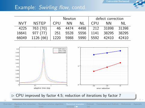
Example: Swirling flow, contd.
Newton defect correctionNVT NSTEP CPU NN NL CPU NN NL4225 763 (70) 46 4474 4498 212 31898 31398
16641 977 (77) 251 5528 5556 1141 38295 3829566049 1126 (66) 1220 5988 5990 5592 42410 42410
0 0.5 1 1.50
0.002
0.004
0.006
0.008
0.01
0.012
0.014
0.016
0.018
0.02 4225 nodes16641 nodes66049 nodes
adaptive time step256 128 64
10−3
10−2
10−1
error reduction
B CPU improved by factor 4.5; reduction of iterations by factor 7
Overview Algebraic flux correction Nonlinear solution algorithm Numerical examples Outlook Conclusions and Outlook References Appendix

16
Universität Dortmund
Example: Swirling flow, contd.
Newton defect correctionNVT NSTEP CPU NN NL CPU NN NL4225 763 (70) 46 4474 4498 212 31898 31398
16641 977 (77) 251 5528 5556 1141 38295 3829566049 1126 (66) 1220 5988 5990 5592 42410 42410
0 0.5 1 1.50
0.002
0.004
0.006
0.008
0.01
0.012
0.014
0.016
0.018
0.02 4225 nodes16641 nodes66049 nodes
adaptive time step0 10 20 30 40 50 60 70 80
10−14
10−12
10−10
10−8
10−6
10−4
number of nonlinear iterations
norm
of n
onlin
ear
resi
dual
B CPU improved by factor 4.5; reduction of iterations by factor 7
Overview Algebraic flux correction Nonlinear solution algorithm Numerical examples Outlook Conclusions and Outlook References Appendix

17
Universität Dortmund
Outlook: Compressible flows, Kuz05b
Divergence Form
∂U∂t +
∑3d=1
∂F d
∂xd= 0 Ad =
∂F d
∂U
Quasi-linear form
∂U∂t +
∑3d=1 Ad ∂U
∂xd= 0
FEM discretization[MC
dudt
]i=
∑j 6=i aij(uj − ui ) aij = rijΛijr
−1ij
Transformation to local characteristic variables makes it possible toperform upwinding and algebraic flux correction as in the scalar case.
M∞ = 3, α = 0, density Mach number
Overview Algebraic flux correction Nonlinear solution algorithm Numerical examples Outlook Conclusions and Outlook References Appendix

18
Universität Dortmund
Grid adaption, Moe06
2048 triangles
0 0.5 1 1.5 2 2.5 3 3.5 40
0.2
0.4
0.6
0.8
1
3503 triangles
0 0.5 1 1.5 2 2.5 3 3.5 40
0.2
0.4
0.6
0.8
1
7194 triangles
0 0.5 1 1.5 2 2.5 3 3.5 40
0.2
0.4
0.6
0.8
1
15664 triangles
0 0.5 1 1.5 2 2.5 3 3.5 40
0.2
0.4
0.6
0.8
1
Density distribution on the final mesh
0 0.5 1 1.5 2 2.5 3 3.5 40
0.5
1
cutline at y = 0.6
0 0.5 1 1.5 2 2.5 3 3.5 4
0.8
1
1.2
1.4
1.6
1.8
2
2.2
grid1 grid2 grid3 grid4
Overview Algebraic flux correction Nonlinear solution algorithm Numerical examples Outlook Conclusions and Outlook References Appendix

19
Universität Dortmund
Conclusions and Outlook
nonlinear high-resolution schemes can be constructed byadding artificial diffusion + limited antidiffusion
implicit flux correction schemes can be combined withalgebraic Newton methods to speed up convergence
Jacobian matrix is approximated by divided differences andassembled efficiently edge-by-edge in a black-box fashion
the sparsity pattern of the Jacobian needs to be extended whichcan be accomplished by standard matrix multiplication
Further research: compressible Euler equations,time-dependent grid adaptation
Overview Algebraic flux correction Nonlinear solution algorithm Numerical examples Outlook Conclusions and Outlook References Appendix

20
Universität Dortmund
References
Kuz05a D. Kuzmin, M.M. Algebraic flux correction I. Scalar conservationlaws. In: Flux-Corrected Transport, Principles, Algorithms, andApplications, D. Kuzmin, R. Lohner, S. Turek (eds.). Springer:Germany, 2005; 155-206
Kuz05b D. Kuzmin, M.M. Algebraic flux correction II. Compressible Eulerequations. In: Flux-Corrected Transport, Principles, Algorithms, andApplications, D. Kuzmin, R. Lohner, S. Turek (eds.). Springer:Germany, 2005; 207-250.
Moe06 M.M., D. Kuzmin. Adaptive mesh refinement for high-resolutionfinite element schemes. IJNMF 52, 2006; 545-569.
Moe07a M.M. Efficient solution techniques for implicit finite elementschemes with flux limiters. IJNMF (in press).
Moe07b M.M, D. Kuzmin, D. Kourounis. Implicit FEM-FCT algorithms anddiscrete Newton methods for transient problems. Tech. Rep. 340,2007, University of Dortmund.
Overview Algebraic flux correction Nonlinear solution algorithm Numerical examples Outlook Conclusions and Outlook References Appendix

21
Universität Dortmund
PID time step control
Normalize relative changes
en =‖un − un−1‖
tol ‖un‖
Reject time step if en > 1
∆tn := β∆tn, 0 < β < 1
Compute new time step
∆tn+1 =
(en−1
en
)kp(
1
en
)kI(
e2n−1
enen−2
)kD
∆tn
Parameters (Valli, Carey, Coutinho)
kP = 0.075, kI = 0.175, kD = 0.01Back
Overview Algebraic flux correction Nonlinear solution algorithm Numerical examples Outlook Conclusions and Outlook References Appendix

22
Universität Dortmund
Multidimensional flux correction
1. Compute the sums of positive/negative antidiffusive fluxes
P+i =
∑j 6=i
max0, fij, P−i =∑j 6=i
min0, fij
2. Define the corresponding upper/lower bounds
Q+i =
∑j 6=i
qij max0, uj − ui, Q−i =
∑j 6=i
qij min0, uj − ui
3. Evaluate the nodal correction factors for positive/negative fluxes
R+i = min1,Q+
i /P+i , R−i = min1,Q−
i /P−i
4. Apply correction factors to the raw antidiffusive fluxes
fi =∑j 6=i
αij fij aij =
minR+
i ,R−j , if fij ≥ 0
minR−i ,R+j , otherwise
Overview Algebraic flux correction Nonlinear solution algorithm Numerical examples Outlook Conclusions and Outlook References Appendix

23
Universität Dortmund
Semi-implicit FCT limiter, Part I
1. Initialization P±i ≡ Q±i ≡ R±i ≡ 0
2.Compute positivity-preserving intermediate low-order solution
u = un + (1− θ)∆tM−1l Lun
3. Evaluate raw antidiffusive flux f nij = ∆tdn
ij (uni − un
j ) and update
P±i := P±i +max
min0, f n
ij , P±j := P±j +max
min0,−f n
ij
4. Update admissible increments for both nodes
Q±i :=
max
minQ±
i , uj − ui, Q±j :=
max
minQ±
j , ui − uj
5. Limite the raw antidiffusive fluxes f nij
R±i := miQ±i /P±i → fij :=
minR+
i ,R−j f nij , ifF n
ij > 0,
minR−i ,R+j f n
ij , otherwise.
Overview Algebraic flux correction Nonlinear solution algorithm Numerical examples Outlook Conclusions and Outlook References Appendix

24
Universität Dortmund
Semi-implicit FCT limiter, Part II
1. Evaluate the target flux
fij = [mij + θ∆td(m)ij ](u
(m)i − u
(m)j )
− [mij − (1− θ)∆tdnij ](u
ni − un
j )
2.Constrain each flux by means of fij
f ∗ij =
minfij ,max0, fij, if fij > 0,
maxfij ,min0, fij, otherwise.
3. Insert the limited antidiffusive flux into the right-hand side
b(m)i := b
(m)i + f ∗ij , b
(m)j := b
(m)j − f ∗ij
Back
Overview Algebraic flux correction Nonlinear solution algorithm Numerical examples Outlook Conclusions and Outlook References Appendix