on a computational approach for the approximate dynamics of averaged variables in nonlinear ode...
TRANSCRIPT
ARTICLE IN PRESS
Journal of the Mechanics and Physics of Solids
54 (2006) 2183–2213
0022-5096/$ -
doi:10.1016/j
CorrespoE-mail ad
www.elsevier.com/locate/jmps
On a computational approach for the approximatedynamics of averaged variables in nonlinear ODEsystems: Toward the derivation of constitutive laws
of the rate type
Amit Acharya, Aarti Sawant
Civil and Environmental Engineering, Carnegie Mellon University, Pittsburgh, PA 15213, USA
Received 24 August 2005; received in revised form 23 March 2006; accepted 25 March 2006
Abstract
A non-perturbative approach to the time-averaging of nonlinear, autonomous ordinary
differential equations is developed based on invariant manifold methodology. The method is
implemented computationally and applied to model problems arising in the mechanics of solids.
r 2006 Elsevier Ltd. All rights reserved.
Keywords: Time-averaging; Coarse graining; Nonlinear ODE systems; Wiggly energy
1. Introduction
We are interested in exploring the possibility of developing a completely defined(i.e. closed) rate-type evolution equation for time averages of prescribed functions of stateof an underlying physical system, the latter assumed to be adequately described by asystem of ordinary differential equations (ODE). We refer to the time averages of theprescribed state functions as coarse variables and the degrees of freedom of the underlyingODE system as fine variables. Of particular interest are the following questions: can such aclosed description be generated at all? If so, is such a description generally adequate for
see front matter r 2006 Elsevier Ltd. All rights reserved.
.jmps.2006.03.007
nding author. Tel.: +1412 268 4566; fax: +1 412 268 7813.
dress: [email protected] (A. Acharya).

ARTICLE IN PRESSA. Acharya, A. Sawant / J. Mech. Phys. Solids 54 (2006) 2183–22132184
probing the evolution of the coarse quantities when appended by an initial condition onthe coarse variables alone?It is shown in this paper that the answer to the first question is in the affirmative, both
conceptually and computationally, with significant practical benefits. As for the secondquestion, the answer is found to be negative in a strict sense. However, from a practicalpoint of view, the proposed method can be shown to be no worse than the philosophy ofphysical experimentation where one might commit oneself to a choice of coarse variablesand the existence of an autonomous, rate-type constitutive equation for these variables andproceed to determine the form of the right-hand side of such an equation by experimentallymonitoring small increments in response out of prescribed coarse states, assuming that acoarse state corresponds to a unique increment out of that state. In fact, a majorcomponent of the long-term, practical objective of this work is to work withexperimentalists in making a choice of coarse variables such that over a broad range ofexperimental trials the incremental response of the chosen set of coarse variables is foundto be unique, once a coarse state has been specified. Of course, our method lays bare thefact that such uniqueness ought not be expected in general, if one were to choose thenumber and type of coarse variables simply on physical grounds and convenience ofmeasurement. Indeed, a simplification of results of Inertial Manifold Theory (Temam,1990) to finite dimensional systems suggests that an autonomous coarse response(corresponding to the class of dissipative fine dynamics that is within the rigorouspurview of Inertial Manifold Theory) is guaranteed if the number of coarse variablesadopted is bounded below by the dimension of the attractor of the fine dynamics. The factthat approximate, consistent, lower-dimensional (than the dimension of the attractor)coarse dynamics can be developed in principle and demonstrated in practice in the contextof small systems displaying complicated dynamics is the subject of our prior work(Acharya, 2005; Sawant and Acharya, 2005), where connections of our approach to relatedwork in the literature are presented. Such consistent coarse dynamics, however, requiresinformation on initial conditions more than what is prescribed merely by a knowledge ofcoarse initial states and displays response characteristic of non-autonomous systems ingeneral, features related to the prediction of memory effects solely as a geometricconsequence of a drastic reduction in degrees of freedom in transitioning from fine tocoarse dynamics. In this paper, ‘memory’ in dynamics refers to the possibility of differentrates of evolution of a set of evolving variables from an identical state for this set. In thissense, such features of coarse dynamics may also be interpreted as stochastic effects.Our overall approach is based on the use of invariant manifolds of the fine dynamics as
proposed in Muncaster (1983), with conceptually and practically non-trivial extensionsmade in Acharya (2005) and Sawant and Acharya (2005). However, these approaches aswell as coarse-graining approaches based on Inertial Manifold Theory (Foias et al., 1988)Center Manifold Theory (Carr and Muncaster, 1983a, b; Roberts, 2003), or theConstructive Methods of Gorban and Karlin (Gorban et al., 2004) have not exploredthe possibility of running time-averages of fine response as coarse variables, perhaps for thereason that such a choice does not fit in naturally into the invariant manifold methodologyfor model reduction. This is so because such averages cannot be defined as functions of theinstantaneous fine state. In this paper, we propose a simple augmentation of the finedynamics that allows such a choice of coarse variables, followed by the use of invariantmanifold methodology for obtaining closed dynamics for the time averages. To ourknowledge, such an approach for dealing with time-averaging is new.
ARTICLE IN PRESSA. Acharya, A. Sawant / J. Mech. Phys. Solids 54 (2006) 2183–2213 2185
Obtaining the effective dynamics of nonlinear ODE systems is a vast field with manyapproaches, as summarized in the excellent review of Givon et al. (2004). Primaryapproaches other than invariant manifold methodology have been the method ofaveraging for Hamiltonian systems (e.g. Neishtadt, 2005, the weak convergence method,Bornemann, 1998) and the projection operator technique (e.g. Chorin et al., 2000). Ourprimary interest being in the mechanics of solids and materials science, we have beenstrongly influenced by the results of Abeyaratne et al. (1996), especially in theirdemonstration of the importance of the averaging of microscopic dynamics, as opposedto the use of averaged energetics, in the construction of effective dynamics. Our main goalis the development of computational methodology based on sound, even if notmathematically rigorous, ideas that can be put to use in the development of constitutiveresponse in the mechanics of solids. We refer to our overall approach as the method ofparametrized locally invariant manifolds (PLIM); the first word in the name is meant toemphasize the practical importance of the parametrization of locally invariant manifoldsof the fine dynamics and, in particular, the evolution of the parameters along finetrajectories on these manifolds. The second word is inserted to emphasize the crucialimportance of allowing for, at least conceptually, the presence of many locally invariantmanifolds in fine phase space corresponding to each local domain of coarse phase space, asdeveloped in Acharya (2005) and Sawant and Acharya (2005).
The conceptual and methodological basis of our multiscale/coarse-graining method iscompared with others, both theoretical and computational, in Acharya (2005) and Sawantand Acharya (2005). The latter paper also documents the computational savings inapproaching coarse-variable evolution by our technique when compared to coarse-evolution through simulation of the fine dynamics. The primary feature of ourcomputational idea that differentiates it from other approaches for multiscale numericsis the suggestion that an appropriate collection of parametrizations of locally invariantmanifolds actually be computed and stored ‘off-line’, a calculation that does not requireevolution of the fine system. With this database in hand, a closed coarse dynamics isdefined that is consistent with the fine (microscopic) dynamics in a well-defined sense, aproperty that is not transparent and/or valid for all multiscale computational approaches.Depending on the choice of coarse variables, a user-input in the procedure, the coarsetheory is computable much more efficiently than the fine theory. As we show in our pastwork and here, this strategy allows us to compute the coarse response of complicatednonlinear systems without special treatment and regardless of whether there exists a‘separation of scale’—e.g., see Sawant and Acharya (2005) for an application to the Lorenzsystem with a choice of coarse variables that neither induces nor exploits any separation ofscales. Of course, our methodology is equally capable of inducing a separation of scale byan appropriate choice of coarse variables and exploiting such a separation as we show inthe examples of this paper, thus providing one avenue for computationally dealing withnonlinear, stiff systems, even oscillatory. As is well known, the ease afforded by theexistence of separation of scales in a problem for doing theory does not necessarily transferto the design of computational algorithms for such, especially for nonlinear stiff problems.
Importantly, our overall approach (Acharya, 2005; Sawant and Acharya, 2005; thispaper) implies that one may not expect an autonomous coarse dynamics simply becausethe coarse variables are chosen as ‘slow’ and/or ‘aggregate’ variables and a separation ofscales exists in this limited, literal, sense. Even more importantly, it suggests a means toachieve, in principle, a consistent coarse dynamics in the absence of a separation of scales

ARTICLE IN PRESSA. Acharya, A. Sawant / J. Mech. Phys. Solids 54 (2006) 2183–22132186
in the sense that the evolution of the fast and slow variables do not decouple, ideas that canbe turned into practice approximately. The latter feature is in contrast to some coarse-graining exercises for ODE, e.g. the homogenization of the associated linear, transportPDE by the method of two-scale convergence as shown in Menon (2002), where the non-uniqueness of the evolution of weak limits (coarse variables) from a specified coarse state isrecovered, but an understanding of the failure at the level of suggesting possibledeterministic remedies is not. While recourse to stochastic models may be the simplestalternative to get some acceptable answers in the absence of a true separation of scales, itmust be realized that, at a fundamental level, the non-autonomous content—both memoryof coarse variables and ‘noise’—of the appropriate stochastic model for coarse-graining adeterministic, nonlinear autonomous system of ODE is intimately linked to understandingof the ‘orthogonal dynamics’ of the eliminated variables and its coupling to the dynamicsof the retained coarse variables, as laid bare by the Mori–Zwanzig Projection OperatorTechnique (Chorin et al., 2002).This paper is organized as follows: the basic theoretical ideas behind our method are
presented in Section 2. Section 3 contains a demonstration of the general strategy throughmodel problems. Scalar and vector gradient flow dynamics with ‘wiggly’ energies due toAbeyaratne et al. (1996) and Menon (2002) are homogenized in time by our method. Whilelow-dimensional, these are complicated problems that do not satisfy any ergodicityhypothesis for the fast dynamics, when suitably phrased as problems of averaging.Next, the macroscopic ‘stress–strain’ response of an atomic chain based on theFrenkel–Kontorova model (e.g., Nabarro, 1987) is computed under monotonic loading. Insolving these problems, it is assumed that full knowledge of fine initial conditions is available.However, in most applications it is reasonable to assume only some limited knowledge, atbest, of the possible fine states corresponding to a coarse initial condition. In Section 4, astrategy is proposed to deal with such situations within our general approach, based purely onconsiderations of practicality. The paper ends with some concluding remarks in Section 5.
2. A simple technique for time-averaging
The autonomous fine dynamics is defined as
df
dttð Þ ¼ H f tð Þð Þ,
f 0ð Þ ¼ f n. ð1Þ
f is an N-dimensional vector of fine degrees of freedom and H is a generally nonlinearfunction of fine states, denoted as the vector field of the fine dynamical system. Eq. (1)2represents the specification of initial conditions. N can be large in principle, and thefunction H rapidly oscillating.Let L be a user-specified function of the fine states producing vectors with m
components whose time averages over intervals of period t can be measured in principleand are of physical interest. Given the fixed time interval t characterizing the resolution ofcoarse measurements in time, a coarse trajectory corresponding to each fine trajectory f( )is defined as the following running time average:
c tð Þ ¼1
t
Z tþt
t
L f sð Þð Þds. (2)

ARTICLE IN PRESSA. Acharya, A. Sawant / J. Mech. Phys. Solids 54 (2006) 2183–2213 2187
Roughly speaking, it is a closed statement of evolution for c that we seek. The goal isunambiguous only after we specify what sort of initial conditions we may want toprescribe. For the purpose of this section, we assume that fine initial conditions are knownwith certainty. Then, the goal is to develop a closed evolution equation for c, i.e. anequation that can be used for evolving c without concurrently evolving (1), correspondingto fine trajectories out of a prescribed set of fine initial conditions.
Clearly,
dc
dttð Þ ¼
1
tL f tþ tð Þð Þ L f tð Þð Þ½ . (3)
If we now introduce a forward trajectory ff ( ) corresponding to a trajectory f ( ) as
f f tð Þ :¼ f tþ tð Þ, (4)
then
df f
dttð Þ ¼ H f f tð Þ
. (5)
Also, given an initial state f we denote by f the state defined as the solution of (1)evaluated at time t. With these definitions in hand, we augment the fine dynamics (1) to
df f
dttð Þ ¼ H f f tð Þ
,
df
dttð Þ ¼ H f tð Þð Þ,
f f 0ð Þ ¼ f ,
f 0ð Þ ¼ f , ð6Þ
and apply invariant manifold techniques to (6). In detail, on an m-dimensional coarsephase space whose generic element we denote as c, we seek functions Gf and G that satisfythe first-order, quasilinear partial differential equations
Pmk¼1
qGIf
qck
1
tLk Gf
Lk Gð Þ
¼ HI Gf
Pmk¼1
qGI
qck
1
tLk Gf
Lk Gð Þ
¼ HI Gð Þ
9>>>>=>>>>;; I ¼ 1 to N, (7)
at least locally in c-space. Assuming that we have such a pair of functions over the domaincontaining the point
c :¼ c 0ð Þ (8)
defined from (1) and (2) which, moreover, satisfies the conditions
Gf cð Þ ¼ f ,
G cð Þ ¼ f , ð9Þ
it is easy to see that a local-in-time fine trajectory defined by
Gf tð Þ :¼ Gf c tð Þð Þ,
G tð Þ :¼ G c tð Þð Þ, ð10Þ
ARTICLE IN PRESSA. Acharya, A. Sawant / J. Mech. Phys. Solids 54 (2006) 2183–22132188
through the coarse local trajectory satisfying
dc
dt¼
1
tL Gf cð Þ
L G cð Þð Þ
,
c 0ð Þ ¼ cn ð11Þ
is the solution of (6) (locally). A solution pair (Gf,G) of (7) represents a parametrization ofa locally invariant manifold of the dynamics (6). By a locally invariant manifold we mean aset of points in phase space such that the vector field of (6) is tangent to the set at all points.Thus, a trajectory of (6) exits a locally invariant manifold only through the boundary ofthe manifold (see more on this geometric interpretation in Sections 2.1 and 5).Also, note that if G
_
f ;G_
and Gf ; G
are two solutions to (7) and (9) on an identicallocal domain in c-space containing cn and c
_ð Þ and c ð Þ are the corresponding coarse
trajectories defined as solutions to (11), then local uniqueness of solutions to (6) implies
G_
f c_
tð Þ
¼: G_
f tð Þ ¼ Gf tð Þ :¼ Gf c tð Þð Þ;
G_
c_
tð Þ
¼: G_
tð Þ ¼ G tð Þ :¼ G c tð Þð Þ:(12)
Thus,
d c_
dttð Þ ¼
dc
dttð Þ locally in time,
c_0ð Þ ¼ c 0ð Þ ð13Þ
from (11), and assuming c_and c are continuous, c
_ c, locally.
Hence, given any pair of mappings Gf, G satisfying (7) and (9) on a domain containing cn,we consider (11) as the consistent, closed theory for the evolution of the coarse variables c.Obstruction to the construction of solutions to (7) is explored in Acharya (2005),providing one reason for seeking multiple local solutions as implemented in Sawant andAcharya (2005).We mention here that the choice of coarse variables (2) can be appended with functions
of the instantaneous fine state of (1) to define more coarse variables. The determiningequations for the G functions and the coarse evolution for these variables are different inform from (7) and (11). This class of coarse variables is the more standard choice inapplications of invariant manifold methodology as outlined, e.g., in Muncaster (1983).Applied loads are introduced as such coarse variables in the model problems of this paperin Section 3.
2.1. Algorithm
The basic algorithmic idea (Sawant and Acharya, 2005), then, is as follows: consider aregion of the phase-space of (1), trajectories/trajectory-segments lying in which one isinterested in coarse-graining. By definition of the forward-shifted variables, this delineatesa region of the phase-space of (6), say R, within which trajectory segments of (6) are to becoarse-grained. One constructs as many pairs of functions (Gf,G ) locally in c-space aspossible, with continuous extensions to the boundaries of their local domains of definitionin coarse space. The ideal limit is when one can ensure that each point of R belongs to therange of at least one such pair. The set of points represented by the range of each such

ARTICLE IN PRESSA. Acharya, A. Sawant / J. Mech. Phys. Solids 54 (2006) 2183–2213 2189
function-pair is a locally invariant manifold for the system (6), i.e. if a fine trajectory wereto be started on this set of points it would stay in this set of points and exit the set onlythrough its boundaries. An easy visualization aid is to consider a generally curved surfacepatch in 3D phase-space. Any trajectory-curve on this surface exits only through the edgesof the surface patch and is unable to do so transversally from any interior point of thissurface patch.
Given a fine initial condition for (6), a choice of a locally invariant manifold is madesuch that this initial condition belongs to it. The coarse theory (11) is now evolved.Tracking fine states on the chosen manifold corresponding to the evolving coarsetrajectory through the evaluation (Gf(c(t)), G(c(t))) geometrically represents the movementalong a curve on the manifold representing a fine trajectory segment. Generally, thecoarse trajectory evolves to a coarse state, say cb, on the boundary of the local coarsedomain of definition of the picked pair (Gf,G ), currently in use in evolving (11). In the idealcase, another pair of solutions to (7) should now be available such that (Gf(cb), G(cb))belongs to its range, and with the choice of this pair, the coarse evolution is furthercontinued. In practice, only a finite number of local solutions of (7) can be computed andnot all points of R can be included in the range of some of these solutions. In such a case,on reaching the boundary of a local coarse domain using the pair (Gf,G), one evaluates thefine state
Gf cbð Þ þ Dt H Gf cbð Þ
;G cbð Þ þ Dt H G cbð Þð Þ
, (14)
where Dt is the time-step of the fine evolution. Suppose that this fine state does not belongto the range of any of the precomputed finite collection of local solutions to (7). Then, onemerely chooses the nearest (in some reasonable metric) available manifold to this fine stateand carries on with the coarse calculation.
In this sense, every choice of a precomputed set of locally invariant manifolds defines anapproximate coarse dynamical system. As more and more manifolds are computed,approaching the ideal limit defined in the previous paragraph, the approximate coarsedynamical system becomes exact. While practically somewhat useless in circumstancesinvolving a large number of fine degrees of freedom, this conceptual exercise is animportant consistency guarantee for our coarse-graining scheme attesting to itscorrectness.
The conceptual importance of the condition (9) for consistent coarse-graining inthe presence of a mathematically arbitrary choice of coarse variables, motivated solelyby physical considerations, cannot be overestimated. As the considerations leadingup to (13) show, it would not be possible to guarantee a correct coarse-graining by simplychoosing any solution of (7) that does not satisfy (9). This raises the unsettling,but inevitable, prospect that the evolution of a small set of physically realistic coarsevariables of autonomous fine dynamics may not be posed correctly as initial valueproblems in the traditional sense whose trajectories are uniquely defined by simplyspecifying coarse initial conditions, and that fine initial conditions might exert someinfluence on coarse dynamics. On the other hand, practical experience with modelingof inelastic response in solid mechanics shows that rate-type coarse equations for arelatively small number of variables representing the coarsening of an enormous collectionof fine entities are often practically adequate for describing macroscopic behavior.These two observations taken together lead us to propose a strategy in Section 4 for

ARTICLE IN PRESSA. Acharya, A. Sawant / J. Mech. Phys. Solids 54 (2006) 2183–22132190
making a choice for the computation of a distinguished set of parametrizations for locallyinvariant manifolds that enable the development of an approximate, rate-type coarsedynamics which, however, would display memory effects for reasons demonstrated inSawant and Acharya (2005).
3. Model problems
In this section we illustrate through examples that the method can be implementedsuccessfully. The first two examples belong to the category where the coarse variables arerunning time averages of the fine variables. We choose two model problems whosedynamics is of the gradient flow type governed by energy functions with smallperturbations. The first example describes the kinetics of a phase transforming material(Abeyaratne et al., 1996) and the second example is a gradient flow in two dimensions(Menon, 2002).The third example belongs to the category where the coarse variables are representative
of a space-time average of a collection of fine degrees of freedom. Specifically, we modelthe behavior of a 1D, discrete chain of atoms in a nonlinear force field, with linear nearest-neighbor interactions.In all the examples presented in this section the fine system is evolved numerically, and
the time-averaged response obtained from the fine system is denoted as the actual/actual
coarse response. The response obtained by evolving the coarse theory is denoted as coarse
response. Both the fine and the coarse theories are evolved discretely in time with identicalnumerical schemes for all the reported comparisons.
3.1. Kinetics of a phase transforming material with wiggly energy
This example is selected from the paper by Abeyaratne et al. (1996), where the evolutionof volume fraction of one of the variants of martensite in a plate subjected to biaxialloading was studied. A fine scale gradient flow model is developed and subsequentlyaveraged to obtain a nonstandard macroscopic kinetic law in closed form through a weakconvergence argument. Due to the restriction of our method to autonomous fine systems,we modify the cyclic loading program of Abeyaratne et al. (1996) slightly to obtain thefollowing fine system of equations describing a gradient flow type kinetic law for thevolume fraction l , under a loading program characterized by stresses s1, s2, s3:
_l ¼ mqW
qll;s1;s2ð Þ; l 0ð Þ ¼ l0,
_s1 ¼ Z s3; _s3 ¼ Z s0 s1ð Þ; s2 tð Þ ¼ constant;
s1 0ð Þ ¼ s01; s3 0ð Þ ¼ s03. ð15Þ
Here s1,s2 represent uniform applied tractions in 1 and 2 directions along the specimenboundary. The variable Z represents the frequency of the periodic loading function and s3is an auxiliary variable introduced to allow an oscillatory response in s1. Fig. 1(a) showsthe periodically varying stress s1 and constant stress s2, along with one of the loadingprograms in Abeyaratne et al. (1996) that is approximated by (15)3,4,5.

ARTICLE IN PRESS
Fig. 1. (a) Loading program s vs. t, (b) energy vs. l, (c) force vs. l, (d) force vs. t.
A. Acharya, A. Sawant / J. Mech. Phys. Solids 54 (2006) 2183–2213 2191
The term m represents the mobility of the system and l0 is the initial volume fraction.The term W is the total energy of the specimen comprising the terms
W load ¼
l2 s21 þ s22
a2 g2 2. a2 þ g2
þ2l s21g
2 s22a2
a2 g2
a2 þ g2
þ s1gþ s2að Þ2
8>>>><>>>>:
9>>>>=>>>>;
1=2
,
W trans:layer ¼ c1l2þ c2 1 l2
,
Wpert ¼ a cosl
; ! 0,
W 0 ¼W load þW trans:layer,
W ¼W 0 þWpert, ð16Þ
ARTICLE IN PRESSA. Acharya, A. Sawant / J. Mech. Phys. Solids 54 (2006) 2183–22132192
where a, g, c1, c2, a, e are parameters. For the physical development of the total energyfunction, consult Abeyaratne et al. (1996).The main observation of their paper related to the effect of the third type of energy Wpert
on the dynamics. This term physically characterizes the tip-splitting phenomenon oftwinned bands within laminates under the loading. Here a is the intensity of theperturbation and e51 is a small parameter characterizing the wavelength of the energywiggles. Fig. 1(b) shows the change in energy due to the contribution of the energy Wpert.The crucial observation due to Abeyaratne et al. (1996) is that this small addition to W0,that averages out to zero, completely changes the force governing the dynamics of theproblem, as seen in Fig. 1(c and d) i.e. a small contribution to energy does not necessarilyconstitute a small contribution to the driving force as can be directly seen by taking aderivative of (16)3 with respect to l. Under the periodic loading program, the volumefraction l shows a fixed or frozen response under varying load in certain regions of loadingand this is attributed (Abeyaratne et al., 1996) to the situation where l gets stuck in a localminimum of W, as can also be inferred from a plot of the forces 1(d).We study the evolution of volume fraction by using W as the energy function with e51
as a fixed parameter. It is important to note that the development of the coarse theory inour approach is non-asymptotic in the sense that it does not depend on taking the limit e-0, a feature that has both merits and demerits in the context of homogenization in time.
Case 1: Cyclic loading program.Following the procedure in Section 2, we define a time averaged volume fraction l using
the definition (2), with L : f 7!f . The corresponding augmented variable as defined in (4)is lf. The fine theory (15) is augmented with an evolution equation corresponding to lf ofthe form
_lf tð Þ ¼ mqW
qllf tð Þ;s1 tþ tð Þ;s2 tþ tð Þ
; lf 0ð Þ ¼ lf 0. (17)
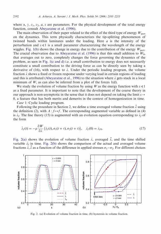
Fig. 2(a) shows the evolution of volume fraction l, averaged l, and the time shiftedvariable lf in time. Fig. 2(b) shows the comparison of the actual and averaged volumefractions l; l as a function of the difference in applied stresses s1s2. For different choices
Fig. 2. (a) Evolution of volume fraction in time, (b) hysteresis in volume fraction.

ARTICLE IN PRESSA. Acharya, A. Sawant / J. Mech. Phys. Solids 54 (2006) 2183–2213 2193
of t (time interval used for averaging), the averaged volume fraction l
profiles(obviously) differ from the fine (l) trajectory, but contain essential features of fine response(frozen l or flat portions seen in Fig. 2).
We choose the averaged volume fraction l and the stresses s1,s3 of the loading programas the coarse variables. Because the solution for s1,s3 in (15) can be expressed explicitly interms of trigonometric functions, it is possible to write down the time-shifted stress termsappearing in (17) in terms of s1(t),s3(t) and functions of the parameter t. Thus the finesystem is not augmented for these variables. We denote the driving force for lf obtained by
this rewriting as dqW=ql
, which is a function of lf,s1,s3 and the parameter t. As the stress
s2 is constant, we treat it as a fixed parameter while computing the locally invariantmanifolds and evolving the coarse dynamics.
We denote the fine variables by functions l ¼ G1 l;s1;s3
and lf ¼ G2 l;s1;s3
. Thesolutions to G1,G2 are obtained by solving the governing equations (18) obtained from theaugmented fine theory:
qG2
qlG2 G1
t
þ
qG2
qs1Zs3 þ
qG2
qs3Z s0 s1ð Þ þ m
dqW
ql
G2;s1;s2; tð Þ ¼ 0,
qG1
qlG2 G1
t
þ
qG1
qs1Zs3 þ
qG1
qs3Z s0 s1ð Þ þ m
qW
qlG1;s1;s2ð Þ ¼ 0. ð18Þ
Here the first term in (18)1,2 corresponds to the left hand side of (7)1,2, with m ¼ 1. Thenext two terms arise due to the dependence of the functions G1,G2 on the other coarsevariables s1,s3. Eq. (18) is solved by using the Least squares finite element method andEI-TC method described in Sawant (2005) and the Appendix of this paper.1
With the solutions obtained for (18), the coarse theory corresponding to equation (11)can be written as,
_l ¼1
tG2 l; s1;s3
G1 l;s1;s3
,
_s1 ¼ Z s3; _s3 ¼ Z s0 s1ð Þ. ð19Þ
To evolve the coarse theory we obtain a consistent initial condition l 0ð Þ by evolving thefine system up to time t. The initial conditions s1(0),s3(0) are selected as in (15).
To illustrate the advantage of using the PLIM method, we compute the coarse responsefrom numerical integration of Eq. (19) by using much larger time steps than the maximaltime step required to obtain the response of the fine system (15). The maximal time-step forthe fine evolution is defined as that value of the time-step for which any time-step smallerthan the maximal one reproduces the same computed response as for the maximal one. Thelatter are subsequently t -time averaged according to (2) for comparison with coarseresponse. We refer to the t -averaged response of a computed fine solution as the actual
coarse response. The ratio of the coarse to fine steps is denoted as c/f. We present thecoarse response computed with c/f ratios of 1, 10, and 100.
Figs. 3 and 4 show the comparisons of coarse response obtained from the coarse andfine theory with parameter values a ¼ 1:0619; g ¼ 1:0231; c1 ¼ 0:017 MPa; c2 ¼
0:0255 MPa; a ¼ 0:025 MPa; m ¼ 5:4 MPa1s1 taken from Abeyaratne et al. (1996).The small parameter e and the time scale t are selected as 0.005 and 2.0 s (200maximal fine
1We thank Dr. Hao Huang for discussions on this matter.
ARTICLE IN PRESS
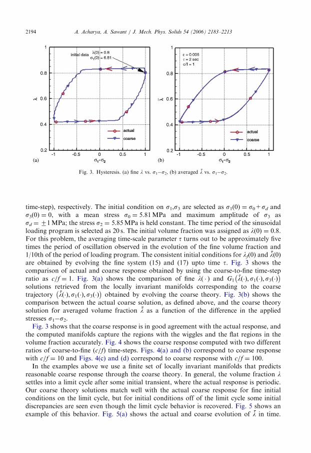
Fig. 3. Hysteresis. (a) fine l vs. s1s2, (b) averaged l vs. s1s2.
A. Acharya, A. Sawant / J. Mech. Phys. Solids 54 (2006) 2183–22132194
time-step), respectively. The initial condition on s1,s3 are selected as s1(0) ¼ s0+sd ands3(0) ¼ 0, with a mean stress s0 ¼ 5.81MPa and maximum amplitude of s3 assd ¼71MPa; the stress s2 ¼ 5.85MPa is held constant. The time period of the sinusoidalloading program is selected as 20 s. The initial volume fraction was assigned as l(0) ¼ 0.8.For this problem, the averaging time-scale parameter t turns out to be approximately fivetimes the period of oscillation observed in the evolution of the fine volume fraction and1/10th of the period of loading program. The consistent initial conditions for lf(0) and l 0ð Þare obtained by evolving the fine system (15) and (17) upto time t. Fig. 3 shows thecomparison of actual and coarse response obtained by using the coarse-to-fine time-stepratio as c/f ¼ 1. Fig. 3(a) shows the comparison of fine l( ) and G1 l ð Þ; s1 ð Þ; s3 ð Þ
solutions retrieved from the locally invariant manifolds corresponding to the coarsetrajectory l ð Þ;s1 ð Þ;s3 ð Þ
obtained by evolving the coarse theory. Fig. 3(b) shows the
comparison between the actual coarse solution, as defined above, and the coarse theorysolution for averaged volume fraction l as a function of the difference in the appliedstresses s1s2.Fig. 3 shows that the coarse response is in good agreement with the actual response, and
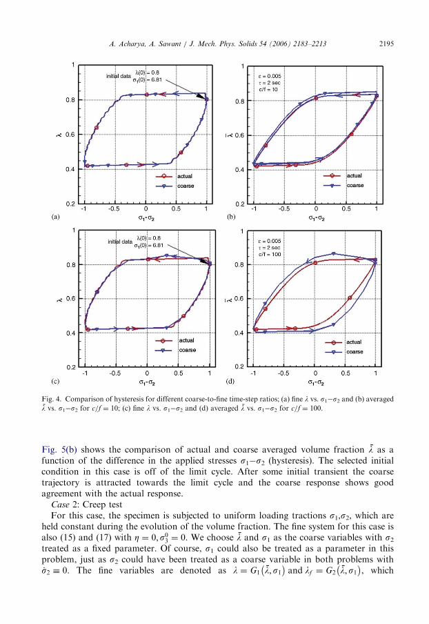
the computed manifolds capture the regions with the wiggles and the flat regions in thevolume fraction accurately. Fig. 4 shows the coarse response computed with two differentratios of coarse-to-fine (c/f) time-steps. Figs. 4(a) and (b) correspond to coarse responsewith c/f ¼ 10 and Figs. 4(c) and (d) correspond to coarse response with c/f ¼ 100.In the examples above we use a finite set of locally invariant manifolds that predicts
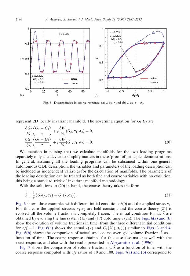
reasonable coarse response through the coarse theory. In general, the volume fraction lsettles into a limit cycle after some initial transient, where the actual response is periodic.Our coarse theory solutions match well with the actual coarse response for fine initialconditions on the limit cycle, but for initial conditions off of the limit cycle some initialdiscrepancies are seen even though the limit cycle behavior is recovered. Fig. 5 shows anexample of this behavior. Fig. 5(a) shows the actual and coarse evolution of l in time.
ARTICLE IN PRESS
Fig. 4. Comparison of hysteresis for different coarse-to-fine time-step ratios; (a) fine l vs. s1s2 and (b) averaged
l vs. s1s2 for c/f ¼ 10; (c) fine l vs. s1s2 and (d) averaged l vs. s1s2 for c/f ¼ 100.
A. Acharya, A. Sawant / J. Mech. Phys. Solids 54 (2006) 2183–2213 2195
Fig. 5(b) shows the comparison of actual and coarse averaged volume fraction l as afunction of the difference in the applied stresses s1s2 (hysteresis). The selected initialcondition in this case is off of the limit cycle. After some initial transient the coarsetrajectory is attracted towards the limit cycle and the coarse response shows goodagreement with the actual response.
Case 2: Creep testFor this case, the specimen is subjected to uniform loading tractions s1,s2, which are
held constant during the evolution of the volume fraction. The fine system for this case isalso (15) and (17) with Z ¼ 0;s03 ¼ 0. We choose l and s1 as the coarse variables with s2treated as a fixed parameter. Of course, s1 could also be treated as a parameter in thisproblem, just as s2 could have been treated as a coarse variable in both problems with_s2 0. The fine variables are denoted as l ¼ G1 l;s1
and lf ¼ G2 l;s1
, which
ARTICLE IN PRESS
Fig. 5. Discrepancies in coarse response: (a) l vs. t and (b) l vs. s1s2.
A. Acharya, A. Sawant / J. Mech. Phys. Solids 54 (2006) 2183–22132196
represent 2D locally invariant manifold. The governing equation for G1,G2 are
qG2
qlG2 G1
t
þ m
qW
qlG2;s1;s2ð Þ ¼ 0,
qG1
qlG2 G1
t
þ m
qW
qlG1;s1;s2ð Þ ¼ 0. ð20Þ
We mention in passing that we calculate manifolds for the two loading programsseparately only as a device to simplify matters in these ‘proof of principle’ demonstrations.In general, assuming all the loading programs can be subsumed within one generalautonomous ODE description, the variables and parameters of the loading description canbe included as independent variables for the calculation of manifolds. The parameters ofthe loading description can be treated as both fine and coarse variables with no evolution,this being a standard trick of invariant manifold methodology.With the solutions to (20) in hand, the coarse theory takes the form
_l ¼1
tG2 l;s1
G1 l; s1
. (21)
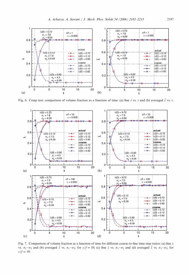
Fig. 6 shows three examples with different initial conditions l(0) and the applied stress s1.For this case the applied stresses s1,s2 are held constant and the coarse theory (21) isevolved till the volume fraction is completely frozen. The initial condition for lf, l areobtained by evolving the fine system (15) and (17) upto time t (2 s). The Figs. 6(a) and (b)show the evolution of volume fractions in time, from the three different initial conditionsfor c/f ¼ 1. Fig. 6(a) shows the actual l( ) and G1 l :ð Þ; s1 :ð Þ
similar to Figs. 3 and 4.
Fig. 6(b) shows the comparison of actual and coarse averaged volume fraction l as afunction of time. The coarse response obtained for this case also matches well with theexact response, and also with the results presented in Abeyaratne et al. (1996).Fig. 7 shows the comparison of volume fractions l, l as a function of time, with the
coarse response computed with c/f ratios of 10 and 100. Figs. 7(a) and (b) correspond to
ARTICLE IN PRESS
Fig. 6. Creep test: comparison of volume fraction as a function of time: (a) fine l vs. t and (b) averaged l vs. t.
Fig. 7. Comparison of volume fraction as a function of time for different coarse-to-fine time-step ratios: (a) fine lvs. s1s2 and (b) averaged l vs. s1s2; for c/f ¼ 10; (c) fine l vs. s1s2 and (d) averaged l vs. s1s2; forc/f ¼ 10.
A. Acharya, A. Sawant / J. Mech. Phys. Solids 54 (2006) 2183–2213 2197

ARTICLE IN PRESSA. Acharya, A. Sawant / J. Mech. Phys. Solids 54 (2006) 2183–22132198
coarse response with c/f ¼ 10, which are in excellent agreement with the actual response.The Figs. 7(c) and (d) correspond to coarse response with c/f ¼ 100, and here the coarsetheory solution shows numerical error due to the larger time steps used. However it showsthe correct trend in the solution.
3.2. 2D gradient system with wiggly energy
This example is selected from the paper by Menon (2002), where a 2D gradient system isstudied with a governing energy function of the following form
W 0 ¼1
2l1y2 þ l2z2
,
Wpert ¼ Rþ rcosz
sin
y
:cos bð Þ þ rsin
z
sin bð Þ; ! 0. ð22Þ
We use the parameter values
R ¼ 2; r ¼ 1; b ¼ p=3; l1 ¼ 1; l2 ¼ 1 (23)
as one representative set suggested in Menon (2002). The small parameter e51 is keptfixed. The fine system for this example takes the form
_y ¼ q W 0 þWpert
qy
¼ Hy y; zð Þ; _z ¼ q W 0 þWpert
@z
¼ Hz y; zð Þ,
y 0ð Þ ¼ y0; z 0ð Þ ¼ z0. ð24Þ
Numerical calculation of trajectories of the fine system indicate that this system has threedistinct parts to its fine phase space shown in Fig. 8, qualitatively consistent with theanalytical conclusions of Menon (2002). Fig. 8 shows two lines r ¼N, r ¼ 0 (dashed),corresponding to the ratio r ¼ _z= _y. These lines divide the fine phase space in zones I and II.
Fig. 8. Schematic representation of the fine phase space.
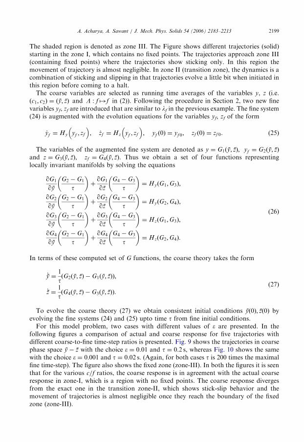
ARTICLE IN PRESSA. Acharya, A. Sawant / J. Mech. Phys. Solids 54 (2006) 2183–2213 2199
The shaded region is denoted as zone III. The Figure shows different trajectories (solid)starting in the zone I, which contains no fixed points. The trajectories approach zone III(containing fixed points) where the trajectories show sticking only. In this region themovement of trajectory is almost negligible. In zone II (transition zone), the dynamics is acombination of sticking and slipping in that trajectories evolve a little bit when initiated inthis region before coming to a halt.
The coarse variables are selected as running time averages of the variables y, z (i.e.c1; c2ð Þ ¼ y; zð Þ and L : f 7!f in (2)). Following the procedure in Section 2, two new finevariables yf, zf are introduced that are similar to lf in the previous example. The fine system(24) is augmented with the evolution equations for the variables yf, zf of the form
_yf ¼ Hy yf ; zf
; _zf ¼ Hz yf ; zf
; yf 0ð Þ ¼ yf 0; zf 0ð Þ ¼ zf 0. (25)
The variables of the augmented fine system are denoted as y ¼ G1 y; zð Þ; yf ¼ G2 y; zð Þ
and z ¼ G3 y; zð Þ; zf ¼ G4 y; zð Þ. Thus we obtain a set of four functions representinglocally invariant manifolds by solving the equations
qG1
qy
G2 G1
t
þ
qG1
qz
G4 G3
t
¼ Hy G1;G3ð Þ;
qG2
qy
G2 G1
t
þ
qG2
qz
G4 G3
t
¼ Hy G2;G4ð Þ;
qG3
qy
G2 G1
t
þ
qG3
qz
G4 G3
t
¼ Hz G1;G3ð Þ;
qG4
qy
G2 G1
t
þ
qG4
qz
G4 G3
t
¼ Hz G2;G4ð Þ:
(26)
In terms of these computed set of G functions, the coarse theory takes the form
_y ¼1
tG2 y; zð Þ G1 y; zð Þð Þ;
_z ¼1
tG4 y; zð Þ G3 y; zð Þð Þ:
(27)
To evolve the coarse theory (27) we obtain consistent initial conditions y 0ð Þ; z 0ð Þ byevolving the fine systems (24) and (25) upto time t from fine initial conditions.
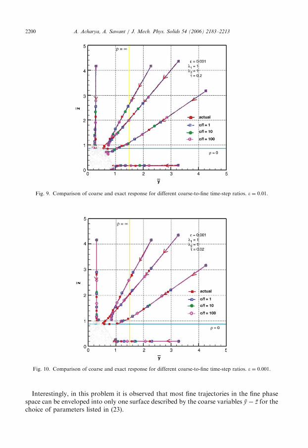
For this model problem, two cases with different values of e are presented. In thefollowing figures a comparison of actual and coarse response for five trajectories withdifferent coarse-to-fine time-step ratios is presented. Fig. 9 shows the trajectories in coarsephase space y z with the choice e ¼ 0.01 and t ¼ 0.2 s, whereas Fig. 10 shows the samewith the choice ¼ 0:001 and t ¼ 0.02 s. (Again, for both cases t is 200 times the maximalfine time-step). The figure also shows the fixed zone (zone-III). In both the figures it is seenthat for the various c/f ratios, the coarse response is in agreement with the actual coarseresponse in zone-I, which is a region with no fixed points. The coarse response divergesfrom the exact one in the transition zone-II, which shows stick-slip behavior and themovement of trajectories is almost negligible once they reach the boundary of the fixedzone (zone-III).
ARTICLE IN PRESS
Fig. 9. Comparison of coarse and exact response for different coarse-to-fine time-step ratios. e ¼ 0.01.
Fig. 10. Comparison of coarse and exact response for different coarse-to-fine time-step ratios. e ¼ 0.001.
A. Acharya, A. Sawant / J. Mech. Phys. Solids 54 (2006) 2183–22132200
Interestingly, in this problem it is observed that most fine trajectories in the fine phasespace can be enveloped into only one surface described by the coarse variables y z for thechoice of parameters listed in (23).

ARTICLE IN PRESS
s oa = a
L(t)k
Linear elastic spring1uη +u2
fixed end
u1 = 0
1 0x =x
sx aη η+1=
substrate
Fig. 11. Schematic representation of a chain of atoms: Frenkel–Kontorova model.
A. Acharya, A. Sawant / J. Mech. Phys. Solids 54 (2006) 2183–2213 2201
3.3. Macroscopic stress– strain curve of an atomic chain
Fig. 11 shows a chain of atoms placed on a substrate that exerts a spatially periodic forceon the atoms derived from a potential of period as. The neighboring atoms are connectedby linear elastic springs (or segments) with stiffness k, and a0 is the distance between theatoms when the springs have zero strain. The chain is fixed at one end and an external loadis applied at the free end. Before application of the load all the atoms are placed in thetroughs of the substrate potential such that as ¼ a0. Thus, the chain is in a stationary statecorresponding to an absolute minimum of potential energy. We refer to this state as a zero-
strain state in rest of this section.The corresponding mechanical model introduced by Frenkel and Kontorova (e.g.,
Braun, 1949), can be derived from the standard Hamiltonian,
h ¼ma
2
Xi
dxi
dt
2
þps
2
Xi
1 cos2p xi x1ð Þ
as
þ
k
2
Xi
xiþ1 xi a0ð Þ2 i ¼ 2 to Zþ 1, ð28Þ
where Z+1 is the total number of particles (atoms). The first term is the kinetic energy,where ma is the mass of each particle and xi is the position of the ith particle in the chain.The second term is a part of the potential energy, which characterizes the interaction of thechain with an external periodic substrate potential, where ps, as are the amplitude andperiod of the potential, respectively. The last potential energy term takes into account alinear coupling between the nearest neighbors of the chain, and is characterized by theelastic constant k and the equilibrium distance of the inter-particle potential, a0, in theabsence of the substrate potential.
From (28), the equations of motion of the particles in the chain subjected to externalload are obtained as
mad2xi
dt2þ
pps
assin
2p xi x1ð Þ
as
k xiþ1 2xi þ xi1ð Þ ¼ F i, (29)
where Fi represents the external load applied at the ith particle. We consider a chain withas ¼ a0 (zero-strain state) as shown in Fig. 11, which helps to replace the position xi withthe displacements ui using xi ¼ (i1)as+ui. The normalized version of (29), in terms of
ARTICLE IN PRESSA. Acharya, A. Sawant / J. Mech. Phys. Solids 54 (2006) 2183–22132202
displacements, is
d2ui
dt2þ sin 2puið Þ k uiþ1 2ui þ ui1ð Þ ¼ F i. (30)
Here, all the forces in (29) are normalized with respect to ratio of the magnitude of the
substrate potential es and its period as i.e. F ¼ F
pps=as
. The actual displacement ui is
normalized as u ¼ u=as; the stiffness is normalized as k ¼ k
pps
a2s
and the time is
normalized as t ¼ t. ffiffiffiffiffiffiffiffiffiffiffiffiffiffiffiffiffiffiffiffi
maa2s
pps
q . For clarity in the rest of the equations the carets are
dropped from the non-dimensional quantities. We introduce the velocities vi and a term aij
representing the elastic force in Eqs. (29)–(30). Thus the normalized fine ODE system thatwe work with is written as follows:
_ui ¼ vi
_vi ¼ sin 2puið Þ þ aij uj þ Fi
)i ¼ 2 to Zþ 1
u1 ¼ 0; v1 ¼ 0 at fixed end; F i ¼ 0 iaZþ 1; F Zþ1 ¼ L tð Þ; _L ¼ f r:
(31)
where L(t) is the normalized external load, applied to Z+1th atom at the end of the chain.We restrict our study to the case of monotonically increasing or decreasing load, i.e.L tð Þ ¼ f 0 þ f rt, where fr is a loading rate.We consider the coarse variable to be a space and time averaged strain. The time
averaged displacement and velocity u; v, are defined as
ui tð Þ ¼1
t
Z tþt
t
ui sð Þds; vi tð Þ ¼1
t
Z tþt
t
vi sð Þds,
i tð Þ ¼ uiþ1 tð Þ ui tð Þ, ð32Þ
where i is the time-averaged strain in ith spring (or segment) coupling the adjacent atomsi, i+1. We define the space and time averaged strain as the number average of time-averaged strains in all Z couplings,
~ tð Þ ¼1
Z
XZi¼1
i tð Þ ¼uZþ1 tð Þ u1 tð Þ
Z. (33)
Here, uZþ1 is a time averaged displacement of the Z+1th particle at the end of the chainwhere the load is applied.We choose the space-time averaged strain ~ and the external force L as the coarse
variables (i.e. c1 ¼ ~;L ¼R L
0 ux dx in (2)) and treat the loading rate fr as a fixed parameter.Using the definition of space-time averaged strain ~ in (33), we obtain an evolutionequation for it as
_~ tð Þ ¼_uZþ1
Z¼
uZþ1 tþ tð Þ uZþ1 tð Þ
t Z. (34)
and (31)5 is the evolution equation for L.Following the recipe set forth in Section 2, the fine system is augmented with time
shifted variables uf, vf corresponding to each particle. The corresponding evolution
ARTICLE IN PRESSA. Acharya, A. Sawant / J. Mech. Phys. Solids 54 (2006) 2183–2213 2203
equations are
_uf
i¼ vf
i; _vf
i¼ sin 2puf
i
þ aij uf
jþ F i; i ¼ 2 to Zþ 1
F i ¼ 0 iaZþ 1; F Zþ1 ¼ L tþ tð Þ ¼ L tð Þ þ tf r; uf
1¼ 0; vf
1¼ 0 at fixed end.
ð35Þ
where F i is the time-shift in the external load applied at ith particle. It should be noted thatwe do not introduce an augmented variable corresponding to the external load, as it can beexpressed as a function of the coarse variable L and the time shift t (35)4.
Now the fine displacements and velocities for each atom are denoted as ukþ1 ¼ Gk ~;Lð Þ,uf
kþ1¼ GkþZ ~;Lð Þ, vkþ1 ¼ Gkþ2Z ~;Lð Þ, and vf
kþ1¼ Gkþ3Z ~;Lð Þ, where k ¼ 1 to Z.
(Note that we do not define the functions G for the degrees of freedom at the fixed end.)With these definitions, a set of 4Z functions are computed by solving the following
governing equations:
qGk
q~G2Z GZ
t
þ
qGk
qLf r ¼ Gkþ2Z;
qGkþZ
q~G2Z GZ
t
þ
qGkþZ
qLf r ¼ Gkþ3Z;
qGkþ2Z
q~G2Z GZ
t
þ
qGkþ2Z
qLf r ¼ sin 2pGkð Þ þ akl Gl þ Fk;
qGkþ3Z
q~G2Z GZ
t
þ
qGkþ3Z
qLf r ¼ sin 2pGkþZ
þ akl GlþZ þ F k:
9>>>>>>>>>>>>>=>>>>>>>>>>>>>;k ¼ 1 to Z.
(36)
A collection of locally invariant manifolds, represented by the functions G, is computedfor different values of loading rate fr. Using this information, the coarse theory takes theform,
_~ ¼1
t ZG2Z ~;Lð Þ GZ ~;Lð Þ
,
_L ¼ f r. ð37Þ
In the computed examples below, we consider a chain of 11 atoms (i.e. Z ¼ 10),subjected to three loadings of the type L tð Þ ¼ f 0 þ f rt corresponding to different values off0 and fr. In all the examples, the initial conditions on displacement and velocity are zero,which correspond to the static zero-strain state described in Fig. 11.
The coarse response is obtained by evolving the coarse theory (37) and a consistentinitial condition ~ 0ð Þ for the coarse variable is obtained by evolving the fine systems (31)and (35) up to a time t. The value of t is selected to be 200 times the maximal time-steprequired for fine evolution, the latter as defined in Section 3.1. Here t is approximately1/3rd (1/5th) of the period of the highest (lowest) mode of free vibration of the linearizedsystem corresponding to (29) about the zero-strain state (i.e. sin(2pui)E2pui, Fi ¼ 0 in(29)). It should be kept in mind that the stiffness of the linearized system changesdrastically as the base state for linearization samples the states encountered duringnonlinear evolution.
ARTICLE IN PRESS
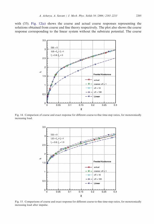
Fig. 13. Force–strain curve for loading and unloading from zero ground state.
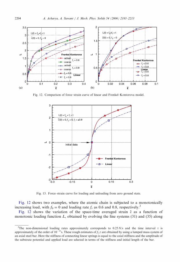
Fig. 12. Comparison of force–strain curve of linear and Frenkel–Kontorova model.
A. Acharya, A. Sawant / J. Mech. Phys. Solids 54 (2006) 2183–22132204
Fig. 12 shows two examples, where the atomic chain is subjected to a monotonicallyincreasing load, with f0 ¼ 0 and loading rate fr as 0.6 and 0.8, respectively.2
Fig. 12 shows the variation of the space-time averaged strain ~ as a function ofmonotonic loading function L, obtained by evolving the fine systems (31) and (35) along
2The non-dimensional loading rates approximately corresponds to 0.25N/s and the time interval t is
approximately of the order of 1011s. These rough estimates of fr,t are obtained by using a lumped mass system of
an axial steel bar. Here the stiffness of connecting linear springs is equal to the axial stiffness and the amplitude of
the substrate potential and applied load are selected in terms of the stiffness and initial length of the bar.
ARTICLE IN PRESSA. Acharya, A. Sawant / J. Mech. Phys. Solids 54 (2006) 2183–2213 2205
with (33). Fig. 12(a) shows the coarse and actual coarse responses representing thesolutions obtained from coarse and fine theory respectively. The plot also shows the coarseresponse corresponding to the linear system without the substrate potential. The coarse
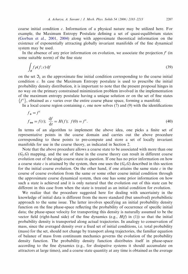
Fig. 14. Comparison of coarse and exact response for different coarse-to-fine time-step ratios, for monotonically
increasing load.
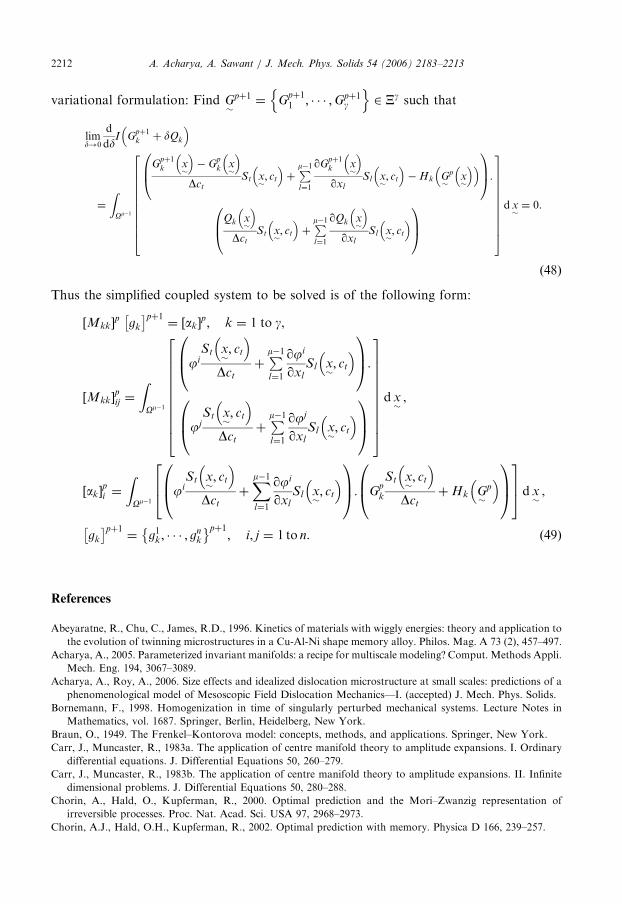
Fig. 15. Comparisons of coarse and exact response for different coarse-to-fine time-step ratios, for monotonically
increasing load after impulse.

ARTICLE IN PRESSA. Acharya, A. Sawant / J. Mech. Phys. Solids 54 (2006) 2183–22132206
responses in this figure are computed by evolving (37) using the same time step required forthe fine system (c/f ¼ 1). It is interesting to observe the similarities of the coarse responsewith macroscopic stress–strain curves, even though the model is extremely simplified.Fig. 12(b) is a magnified version of Fig. 12(a) which shows behavior similar to that in thelinear elastic regime and stage II–stage III transition in work-hardening response for elasticplastic solids. For the cases with initial configuration of zero-strain state, the force-straincurve is symmetric in tension and compression as shown in Fig. 13.Fig. 14 shows the coarse response computed by evolving the coarse theory with larger
time steps, with coarse to fine time steps ratios (c/f) of 10 and 100. This plot also showsgood agreement between coarse and actual coarse results for all (c/f) ratios. Fig. 15 showsthe coarse response for a third example, where the chain is loaded impulsively with f0 ¼ 1.5and subsequently the load is increased monotonically at a constant loading rate fr ¼ 0.8.This plot shows the coarse responses for (c/f) ratios of 1, 10 and 100. The force–straincurve is similar to the work-hardening region, as the applied impulsive load is much largerthan the yielding loads.
4. Strategy for defining an approximate rate-type coarse dynamics: a practical expedient
The considerations in Section 2 indicate that the ideal collection of parametrizations(mappings) of locally invariant manifolds is one where each point of the fine phase-spaceregion of interest is an element of the range of at least one parametrization in thecollection. For a fine dynamics with a large number of degrees of freedom with a choice ofcoarse variables that are few in number, attaining this goal is impractical. It is also truethat empirical, memory-less, rate-type constitutive theories for the nonlinear, inelasticbehavior of solids have been reasonably successful as modeling tools. In addition, it shouldbe kept in mind that procedures like those of Enskog, Chapman, Grad, and Truesdell andMuncaster3 in the Kinetic Theory of Gases, the prototypical example of coarse-graining anonlinear dynamical systems with many degrees of freedom, commit to the completedetermination of a strict rate-type coarse theory that would conceptually paralleldeveloping (11) with only one local solution of (7). Such a choice may be physicallyinterpreted as the assumption that the evolution of coarse states is not sensitive to fineinitial conditions, while low-dimensional dynamics indicate that this assumption cannot bevalid in general (e.g., Sawant and Acharya, 2005). Finally, in many practical situationsexact knowledge of fine initial conditions consistent with an observable coarse one maysimply not be available.The above reasons motivate us to propose the following compromise for the calculation
of a set of parametrizations for use in the coarse theory. Arbitrarily fix a coarse state c,considered as a representative coarse initial condition. Denote by Ic the set of fine statesconsistent with this coarse initial condition:
Ic ¼ f 0 : c ¼
Z t
0
L f sð Þð Þds;df
dt¼ H fð Þ; f 0ð Þ ¼ f 0
. (38)
For each c, let a probability density function, r(f, c), be defined on the set Ic (with obviousextension to the whole of the fine phase space, F, of (1)) that reflects the probability of afine state being the actual fine initial condition realized, corresponding to the observed
3The reader is referred to Truesdell and Muncaster (1980) for an excellent exposition of all of these procedures.
ARTICLE IN PRESSA. Acharya, A. Sawant / J. Mech. Phys. Solids 54 (2006) 2183–2213 2207
coarse initial condition c. Information of a physical nature may be utilized here. Forexample, the Maximum Entropy Postulate defining a set of quasi-equilibrium states(Gorban et al., 2001, 2004) along with approximate theoretical information on theexistence of exponentially attracting globally invariant manifolds of the fine dynamicalsystem may be used.
In the absence of any prior information on evolution, we associate the projection fc (insome suitable norm) of the fine stateZ
Ff r f ; cð Þdf (39)
on the set Ic as the approximate fine initial condition corresponding to the coarse initialcondition c. In case the Maximum Entropy postulate is used to prescribe the initialprobability density distribution, it is important to note that the present proposal hinges inno way on the primary constrained minimization problem involved in the implementationof the maximum entropy postulate having a unique solution or on the set of fine states
f c
, obtained as c varies over the entire coarse phase space, forming a manifold.In a local coarse region containing c, one now solves (7) and (9) with the identifications
f n ¼ f c
f nn ¼ f tð Þ;df
dt¼ H fð Þ; f 0ð Þ ¼ f c. ð40Þ
In terms of an algorithm to implement the above idea, one picks a finite set ofrepresentative points in the coarse domain and carries out the above procedurecorresponding to these points to pre-compute and store a set of locally invariantmanifolds for use in the coarse theory, as indicated in Section 2.
Note that the above procedure allows a coarse state to be associated with more than one(Gf,G) mapping, and the use of these in the coarse theory can result in different coarseevolution out of the single coarse state in question. If one has no prior information on howa coarse state c is attained by the system, then one uses the (Gf,G) described in this sectionfor the initial coarse evolution. On the other hand, if one attains the same state c in thecourse of coarse evolution from the same or some other coarse initial condition throughthe approximate coarse dynamical system, then one has some prior information on howsuch a state is achieved and it is only natural that the evolution out of this state can bedifferent in this case from when the state is treated as an initial condition for evolution.
We realize that the procedure suggested here for dealing with uncertainty in theknowledge of initial data is different from the more standard (but unsolved) probabilisticapproach to the same issue. The latter involves specifying an initial probability densityfunction on the fine phase-space reflecting the probability of occurrence of specific initialdata; the phase-space velocity for transporting this density is naturally assumed to be thevector field (right-hand side) of the fine dynamics (e.g., H(f) in (1)) so that the initialprobability density is transported along actual trajectories. In analogy to conservation ofmass, since the averaged density over a fixed set of initial conditions, i.e. total probability(mass) for the set, should not change by transport along trajectories, the familiar equationof balance of mass from continuum mechanics governs the evolution of the probabilitydensity function. The probability density function distributes itself in phase-spaceaccording to the fine dynamics (e.g., for dissipative systems it should accumulate onattractors at large times), and a coarse state quantity at any time is obtained as the average

ARTICLE IN PRESSA. Acharya, A. Sawant / J. Mech. Phys. Solids 54 (2006) 2183–22132208
of the corresponding coarse state function on phase-space weighted by the evolvingprobability density function. While we see obvious pros and cons for both approaches, athorough comparative evaluation awaits further research.
5. Concluding remarks
Regardless of the coarse-graining technique employed, it is perhaps fair to say that givena fine dynamics containing N degrees of freedom, a closed, dynamics for M(MpN) coarsevariables, requiring initial data on only these M variables and valid for all t-N, ispossible if there exists an M-dimensional globally invariant manifold in the N-dimensionalphase space of the fine system. In essence, our method shows that an m-dimensional(moM) closed, coarse dynamics can also be defined, but one which requires initialconditions on at least M variables to be exact. Such an exact m-dimensional dynamicsdisplays memory effects in coarse variables. These general conclusions on the qualitativenature of exact, reduced coarse dynamics, i.e. memory and requirement of fine initialconditions, are similar to those obtained from the Mori–Zwanzig Projection OperatorTechnique (e.g. Chorin et al., 2000) of non-equilibrium statistical physics, but here reachedthrough completely different logical arguments of a simple geometric nature. We takesatisfaction in the fact that our entire procedure can be understood with only abackground in multivariable calculus, the elementary theory of ordinary differentialequations and equally elementary background in the theory of first-order, quasilinear,partial differential equations. The crux of the conceptual implementation of the methodinvolves ‘filling up’ an M-dimensional manifold with m-dimensional, locally invariantsubmanifolds, in the sense of coverings. A useful geometric picture is to think of a region of3D space being filled by an infinite collection of 2D, possibly intersecting, surface patches;almost all (1D) aperiodic fine trajectories initiated in the 3D region run along thesepatches, jumping appropriately from one to another, twisting and turning to cover thethree-dimensional region densely.The practical implementation of our method involves, obviously, the computation of a
finite collection of m-dimensional, locally invariant submanifolds and consequently, someerror is to be expected. But the value of the fact that the source of this error is transparentin the methodology suggesting, at least, brute-force improvements to it in the form of thepre-computation and storage of a more extensive set of locally invariant manifolds, is notto be underestimated. These ideas are demonstrated in the context of the Lorenz system inSawant and Acharya (2005). Moreover, it is not completely clear whether the validity ofthe coarse-grained dynamics for the limit t-N is necessary for computational coarsegraining schemes so that the necessity of the existence of M-dimensional fine, globally
invariant manifolds may become irrelevant and one might be able to gainfully apply ourtechnique for parametrizing particular bounded regions of fine phase space that finetrajectories to be coarse grained could very well exit. The thrust of our work in this paper isto show that our strategy can actually be executed in quite difficult nonlinear problemsinvolving homogenization in time. Our results also show that the proposed approach canserve to set up approximate models of coarse behavior at least in the neighborhood of acollection of specific fine trajectories that may be deemed to be especially important onphysical grounds, as in the example of the atomic chain.As for error control in practical problems, we appeal to making a good choice of the
coarse variables, in particular, on the knowledge that the chosen coarse variables are

ARTICLE IN PRESSA. Acharya, A. Sawant / J. Mech. Phys. Solids 54 (2006) 2183–2213 2209
physical, macroscopic observables that more-or-less evolve in a state-dependent way, i.e.come close to forming a set capable of parametrizing a physically relevant invariantmanifold of the fine dynamics. The main task then, is to derive an approximate right-handside of the coarse evolution equation. We emphasize here that our modest goal is simplythe determination of the right-hand side, given the definition of the coarse variables alongfine trajectories. An equally valid question is understanding the process of making thischoice of coarse variables with a view to making the best possible one, but as one of themost important results from Inertial Manifold Theory shows, this can lead to questions ofestimating the geometry, in particular, the fractal dimension, of complicated sets(attractors) in fine phase-space that may set a lower bound on the number of coarsevariables.
Running space-time averaging of PDE systems (e.g. Acharya and Roy (2006) for anexample related to dislocation mechanics in crystalline materials) naturally furnishexamples of the type of coarse variables we seek. With some physically motivatedapproximations related to the time dependence of boundary conditions on the averagingdomain, such averaging problems can be fitted into our framework. Of course, there is noguarantee in such a case that the adopted coarse variables ought to display more-or-lessmemory-less behavior and that the approximations related to the boundary conditions areappropriate, and a future challenge for us is to apply, evaluate, and improve themethodology developed herein for such problems. In the case of a transition fromdislocation mechanics to plasticity, it would also be interesting to compare the resultingdynamics to the autonomous dynamics deduced by Puglisi and Truskinovsky (2005) viaapproximate homogenization.
Acknowledgments
Support for this work from the Program in Computational Mechanics of the US ONR(N00014-02-1-0194) and the US AFOSR (F49620-03-1-0254) is gratefully acknowledged.
Appendix A. Explicit integration of PDE in the direction of the time-like coarse variable
(EI-TC)
This section gives a general procedure for solving the PDE that arises in the PLIMmethod by explicit integration in the direction of time-like coarse variable (Sawant, 2005).This procedure was used to compute the locally invariant manifolds for the modelproblems in Section 3.
Consider an augmented/non-augmented fine dynamical system (e.g. (6), (15)+(17),
(24)+(25), (31)+(35)). Let f
¼ f 1; . . . ; f g
n obe the generic state of the fine dynamical
system, e.g. f
corresponding to (1)–(6) consists of the list (f, ff). Let c¼ c1; . . . ; cm
be the
selected coarse variables. The unknown functions representing the locally invariant
manifolds corresponding to f
are denoted as G
c
¼ f
. Let the governing equation for
kth unknown function Gk, similar to (7) described in Section 2 (e.g. (18), (26), (36)), be of

ARTICLE IN PRESSA. Acharya, A. Sawant / J. Mech. Phys. Solids 54 (2006) 2183–22132210
the form,
Xml¼1
qGk
qcl
Sl c; G
c
¼ Hk G
c
; f k ¼ Gk c
; k ¼ 1 to g, (41)
where, the term Sl represents the rhs (right-hand side) of the evolution equation for the lth
coarse variable, e.g. (11), (19), (27), (37). In the constraint equation (41)2, f k is the imposed
value for the kth function Gk at coarse state c
.
Note that, G
corresponds to all the unknown functions to be solved using (41). These should
not be confused with G,Gf in Section 2. For clarity the carets over all the terms are dropped in
rest of this section.
To solve the governing equations (41), we choose a ‘time-like’ variable from the set c,
denoted by ct, say ct ¼ cm, 1pmpm. One requirement on this choice is that the rhs or S ofits evolution equation, is non-zero (at least at all points of the initial hyperplane m ct ¼ ct ).The remaining set of coarse variables are defined as,
x¼ x1; ;xm1
. (42)
The discrete approximation for the kth function representing the locally invariantmanifolds, Gk x
; ct
, is of the following form:
Gk x; ct
Xn
i
gik ctð Þji x
; x2 Om1. (43)
Here n is the total number of discrete nodes in the reduced coarse phase space Om1, xk isthe kth independent coarse variable and gi
k ctð Þ is the value of the function Gk evaluated atnode x
i at ‘time’ ct. A typical governing equation and constraint equation for Gk can bewritten as,
qGk
qct
x; ct
St x; ct;G
x; ct
þXm1l¼1
qGk
qxl
x; ct
Sl x; ct;G
x; ct
¼ Hk G
x; ct
; k ¼ 1 to g, ð44Þ
where St is the non-zero rhs of the evolution equation for coarse variable ct. It is importantto note that due to the requirement of non-zero St, one has to choose a different coarsevariable as ct in case we reach a point or curve where St ¼ 0.The derivative of Gk with respect to ct is approximated by
qG
qct
x; ct
G x; ct þ Dct
G x
; ct
Dct
, (45)
and this discretization is substituted in the governing equation (44) to compute thesolution. For this approach, consistent data is imposed at an initial step ct over the coarse

ARTICLE IN PRESSA. Acharya, A. Sawant / J. Mech. Phys. Solids 54 (2006) 2183–2213 2211
domain Om1 as
f k ¼ Gk x; ct
; k ¼ 1 to g. (46)
The following figure illustrates the above discretization for the model problem 2 of 2Dgradient system with wiggly energy. The augmented fine system consists of four finevariables y, yf, z, zf, i.e. g ¼ 4. The coarse variables are c
¼ y; z
, i.e. m ¼ 2.
y
z
p 1p +
i
1i +
1i −
( )zΩ
*y
( ) ( )( ) ( )
* * *1
*
*
* * *3
2
4
, , , ,
, , ,
f
f
y G z y y G z y
z G z y z G z y
= =
= =
evolution in y direction
*. along I C y y z= ∀ :
Schematic diagram for evolution in the direction of time-like coarse variable (EI-TC).Here we choose say y as the time-like variable and the unknown functions Gk y; zð Þ are
discretized in z direction using finite elements. The solutions to Gk y; zð Þ are computed bymarching in the y direction, where y ¼ y is the initial curve over which consistent data isimposed that serve as initial conditions for the ‘time’ marching scheme.
From (44)–(46), we construct the following quadratic functional that is defined in termsof the L2 norms of the equation residuals:
I : Xg! R
I G
pþ1
¼
ZOm1
Xgk¼1
Gpþ1k x
G
pk x
Dct
St x; ct;G
p x
þPm1l¼1
qGpþ1k x
qxl
Sl x; ct;G
p x
Hk G
p x
0BBBBBB@
1CCCCCCA
28>>>>>>><>>>>>>>:
9>>>>>>>=>>>>>>>;dx,
ð47Þ
where Gpk x
;Gpþ1
k x
are the values of the function Gk x
evaluated at pth and p+1th
step in the time-like direction and the terms S, H are computed from the G
p x
at pth step.
Thus the EI-TC method is a linearized numerical scheme with consistent mixture offorward and backward Euler schemes.
A necessary condition that G
pþ1 2 Xg is a minimizer of the functional I is that its first
variation vanishes at G
pþ1 for all admissible Q
2 Xg. This leads to the least-squares
ARTICLE IN PRESSA. Acharya, A. Sawant / J. Mech. Phys. Solids 54 (2006) 2183–22132212
variational formulation: Find G
pþ1 ¼ Gpþ11 ; ;Gpþ1
g
n o2 Xg such that
limd!0
d
ddI G
pþ1k þ dQk
¼
ZOm1
Gpþ1k x
G
pk x
Dct
St x; ct
þPm1l¼1
qGpþ1k x
qxl
Sl x; ct
Hk G
p x
0B@1CA:
Qk x
Dct
St x; ct
þPm1l¼1
qQk x
qxl
Sl x; ct
0B@1CA
26666666664
37777777775d x¼ 0.
ð48Þ
Thus the simplified coupled system to be solved is of the following form:
Mkk½ p gk
pþ1¼ ak½
p; k ¼ 1 to g,
Mkk½ pij ¼
ZOm1
jiSt x; ct
Dct
þPm1l¼1
qji
qxl
Sl x; ct
0B@1CA:
jjSt x; ct
Dct
þPm1l¼1
qjj
qxl
Sl x; ct
0B@1CA
26666666664
37777777775dx,
ak½ pi ¼
ZOm1
jiSt x; ct
Dct
þXm1l¼1
qji
qxl
Sl x; ct
0B@1CA: G
pk
St x; ct
Dct
þHk G
p 0B@
1CA264
375dx,
gk
pþ1¼ g1
k; ; gnk
pþ1; i; j ¼ 1 to n. ð49Þ
References
Abeyaratne, R., Chu, C., James, R.D., 1996. Kinetics of materials with wiggly energies: theory and application to
the evolution of twinning microstructures in a Cu-Al-Ni shape memory alloy. Philos. Mag. A 73 (2), 457–497.
Acharya, A., 2005. Parameterized invariant manifolds: a recipe for multiscale modeling? Comput. Methods Appli.
Mech. Eng. 194, 3067–3089.
Acharya, A., Roy, A., 2006. Size effects and idealized dislocation microstructure at small scales: predictions of a
phenomenological model of Mesoscopic Field Dislocation Mechanics—I. (accepted) J. Mech. Phys. Solids.
Bornemann, F., 1998. Homogenization in time of singularly perturbed mechanical systems. Lecture Notes in
Mathematics, vol. 1687. Springer, Berlin, Heidelberg, New York.
Braun, O., 1949. The Frenkel–Kontorova model: concepts, methods, and applications. Springer, New York.
Carr, J., Muncaster, R., 1983a. The application of centre manifold theory to amplitude expansions. I. Ordinary
differential equations. J. Differential Equations 50, 260–279.
Carr, J., Muncaster, R., 1983b. The application of centre manifold theory to amplitude expansions. II. Infinite
dimensional problems. J. Differential Equations 50, 280–288.
Chorin, A., Hald, O., Kupferman, R., 2000. Optimal prediction and the Mori–Zwanzig representation of
irreversible processes. Proc. Nat. Acad. Sci. USA 97, 2968–2973.
Chorin, A.J., Hald, O.H., Kupferman, R., 2002. Optimal prediction with memory. Physica D 166, 239–257.
ARTICLE IN PRESSA. Acharya, A. Sawant / J. Mech. Phys. Solids 54 (2006) 2183–2213 2213
Foias, C., Sell, G.R., Temam, R., 1988. Inertial manifolds for nonlinear evolutionary equations. J. Differential
Equations 73, 309–353.
Givon, D., Kupferman, R., Stuart, A., 2004. Extracting macroscopic dynamics: model problems and algorithms.
Nonlinearity 17, R55–R127.
Gorban, A.N., Karlin, I.V., Ilg, P., Ottinger, H.C., 2001. Corrections and enhancements of quasi-equilibrium
states. J. Non-Newtonian Fluid Mech. 96, 203–219.
Gorban, A.N., Karlin, I.V., Zinovyev, A.Yu, 2004. Constructive methods of invariant manifolds for kinetic
problems. Phys. Rep. 396, 197–403.
Menon, G., 2002. Gradient systems with wiggly energies and related averaging problems. Arch. Rat. Mech. Anal.
162, 193–246.
Muncaster, R.G., 1983. Invariant manifolds in mechanics I: the general construction of coarse theories from fine
theories. Arch. Rat. Mech. Anal. 84, 353–373.
Nabarro, F.R.N., 1987. Theory of Crystal Dislocations. Dover, New York.
Neishtadt, A., 2005. Probability phenomena in perturbed dynamical systems. In: Gutkowski, W., Kowalewski,
T.A. (Eds.), Mechanics of the 21st Century, Proceedings of the 21st International Congress of Theoretical and
Applied Mechanics. Springer, Warsaw, pp. 241–261.
Puglisi, G., Truskinovsky, L., 2005. Thermodynamics of rate-independent plasticity. J. Mech. Phys. Solids 53,
655–679.
Roberts, A.J., 2003. Low-dimensional modeling of dynamical systems applied to some dissipative fluid dynamics.
In: Ball, R., Akhmediev, N. (Eds.), Nonlinear dynamics from lasers to butterflies, Lecture Notes in Complex
systems. World Scientific, Singapore 1, pp. 257–313.
Sawant A., Acharya, A., 2005. Model reduction via parameterized locally invariant manifolds: some examples.
Comput. Methods Appl. Mech. Eng. (accepted), http://www.arxiv.org/abs/math-ph/0412022.
Sawant, A., 2005. Parameterized locally invariant manifolds: a tool for multiscale modeling. Ph.D. Thesis,
Carnegie Mellon University.
Temam, R., 1990. Inertial manifolds. Math. Intelli. 12, 68–74.
Truesdell, C.A., Muncaster, R.G., 1980. Fundamentals of Maxwell’s Kinetic Theory of a Simple Monatomic Gas.
Academic Press, New York.