okladka miatluk druk - politechnika białostocka
TRANSCRIPT


Reviewers:
dr hab. eng. Mariusz Giergiel, prof.
prof. Norbert Kruger
Editorial content:
Olga Turłaj
© Copyright by Printing House of Bialystok University of Technology, Bialystok 2017
ISBN 978-83-65596-31-4 ISBN 978-83-65596-32-1 (eBook)
The publication is available on license Creative Commons Recognition of authorship -
Non-commercial use - Without dependent works 4.0 (CC BY-NC-ND 4.0)
Full license content available on the site creativecommons.org/licenses/by-nc-
nd/4.0/legalcode.pl
The publication is available on the Internet on the site of the Printing House of Bialystok
University of Technology
Technical editing, binding:
Printing House of Bialystok University of Technology
Printing:
„UNI-DRUK” Wydawnictwo i Drukarnia Sp. J.
Edition: 43 copies
Printing House of Bialystok University of Technology
ul. Wiejska 45C, 15-351 Białystok
tel.: 85 746 91 37, fax: 85 746 90 12
e-mail: [email protected]
www.pb.edu.pl

3
CONTENT
Conventional signs and notions ............................................................................. 5
PREFACE .............................................................................................................. 7
1. INTRODUCTION-OVERVIEW OF DESIGN METHODS AND MODELS . 9
2. GEOMETRIC MODELS IN DESIGN SYSTEMS ........................................... 19
3. THEORETICAL BASIS OF THE DESIGN METHOD ................................... 28
3.1. Formal model of hierarchical mechatronic system .................................... 28
3.1.1. Aggregated dynamic realization …................................................. 32
3.1.2. Structure .......................................................................................... 37 3.1.3. Coordinator ..................................................................................... 38
3.2. Canonical model of coordinator ................................................................. 44
3.2.1. Presentation of coordinating element .............................................. 47
3.2.2. Process of coordination ................................................................... 51
3.2.3. Description of coordinator environment ......................................... 54
3.2.4. Performance of the design task of mechatronic systems ................. 57
3.3. Metrical characteristics of hierarchical mechatronic systems .................... 59
3.3.1. Levels of mechatronic systems ....................................................... 59
3.3.2. Numeric positional system .............................................................. 61
3.3.3. Measuring units of mechatronic objects .......................................... 71
Preliminary conclusions ............................................................................ 72
4. DESCRIPTION OF THE DESIGN METHOD ................................................. 74
4.1. General geometric characteristics of mechatronic objects ......................... 77
4.2. Numerical characteristics of mechatronic objects ...................................... 80
4.3. Hierarchical geometric representation of mechatronic objects .................. 82
4.3.1. Conditional point ............................................................................ 83
4.3.2. Conditional line .............................................................................. 84
4.3.3. Conditional surface …..................................................................... 86
4.3.4. 3D Object ........................................................................................ 88
4.3.5. Interconnections coordination of geometric elements
of mechatronic objects .................................................................... 90
4.4. Procedures of geometric design of mechatronic objects ............................ 91
4
4.4.1. Coordinator actions with geometric elements of mechatronic
objects ........................................................................................... 91
4.4.2. Geometric synthesis ...................................................................... 92
4.4.3. Motion design and deformation as analysis tasks ......................... 96
Preliminary conclusions .......................................................................... 103
5. CONCEPTUAL DESIGN OF BIOMECHATRONIC SURGICAL
ROBOT SYSTEM …...................................................................................... 104
5.1. Conceptual formal model of surgical robot system …............................. 105
5.2. Realization of coordination – design and control – tasks ….................... 114
Preliminary conclusions ….............................................................................. 119
6. CONCEPTUAL MODEL OF BIOLOGICALLY INSPIRED ROBOT .......... 121
6.1. Conceptual model of dinosaur robot ......................................................... 121
6.2. Robot motion design ................................................................................. 125
6.3. Assembly of dinosaur robot parts ............................................................. 126
Preliminary conclusions ................................................................................... 129
7. HUMAN MOTON DESIGN USING HIERARCHICAL SYSTEMS
METHOD ………............................................................................................. 130
7.1. Coordination task formulation …….......................................................... 131
7.2. Definition of human movements and deformations .................................. 133
7.3. Computer design of human motion ........................................................... 134
7.3.1. Algorithm of human motion design ……........................................ 135
7.3.2. Computer design of human sitting-standing-up movements ...…... 138
7.4. Description of the laboratory experiment ……......................................... 143
Preliminary conclusions and results ……........................................................ 149
8. DESIGN AND TESTING OF ELECTRONIC CIRCUIT BOARDS .............. 152
8.1. Geometric construction of circuit board …............................................... 153
8.2. Stages of PCB interconnections quality testing ….................................... 157
Preliminary conclusions …............................................................................... 161
9. DESIGN AND CONTROL OF MCM CUTTING MACHINE ....................... 162
9.1. MCM conceptual model ........................................................................... 163
9.2. Design tasks ….......................................................................................... 171
9.3. MCM motion design and simulation – Robwork Studio
integration ................................................................................................. 175
Preliminary conclusions ................................................................................... 179
CONCLUSION .................................................................................................... 180
Acknowledgments ................................................................................................ 187
REFERENCES ..................................................................................................... 188
5
Conventional signs and notions
Abbreviations and notions:
MS – mechatronic system,
MO – mechatronic object,
MP – mechatronic process,
CD – conceptual design,
DD – detailed design,
CS – conceptual studies,
PC – personal computer,
GO – geometric object,
CAD – computer aided design,
CAE – computer aided engineering,
CIM – computer integrated manufacturing,
KBE – knowledge based engineering,
MDE – model-driven engineering,
FBS – function-behavior-structure,
FCBS – function-cell-behaviour-structure,
FKC – functional knowledge cell,
B-R – boundary representation,
CSG – constructive solid geometry,
ACS – automated computer system,
HS – hierarchical system,
DE – differential equations,
CG – computational geometry,
SRS – surgical robot system,
TKA – total knee arthoplasty,
MCM – manhole cutting machine,
PCB – printed electronic circuit board,
Coordination – systems design and control processes,
Aed – formal analogous of two-level system with dynamic objects,
6
Sings and variables:
X – input,
Y – output, S – system of level l, So
– object of level l,
S – process of system S of level l,
S – environment of system S ,
– structure of system S , 0S – coordinator of system S ,
– aggregated dynamic presentation of system S , – reaction of system S ,
– function of states transition of system S ,
SL – numerical positional system,
– output function of coordinator (coordination strategy),
tt’ – time interval [t, t’],
– coordination signal and sub-systems connections,
w – feedback signal.

7
PREFACE
This book presents the systemic model and coordination technology of hierarchical
systems for conceptual design of mechatronic and other engineering objects. The
conceptual model creation of the mechatronic system (MS) being designed is the
actual task which is performed in the frames of automation and robotics, mecha-
tronics, engineering design, computer integrated manufacturing (CIM), computer
aided design (CAD) and other related subject fields. Conceptual model of the de-
signed object is usually created before generating concrete mathematical models
necessary for design tasks performing at the detailed design phase of the object life
cycle [1].
Among the widespread models and methods which are usually used at the
conceptual and detailed design phases are the following ones. Models of classical
mathematics – discrete and continuous – successfully used to model the dynamics
or structure of the object being designed, but do not solve the basic problem of
design: do not link the structure of the object and its function. Models of artificial
intelligence are most commonly used when describing the structure of the designed
object and design knowledge representation. Solving some specific design prob-
lems, these models remain one-level at its core and do not take into account the
dynamics of the object being designed and therefore do not perform the general
design task in one common theoretical basis. For the case of logical-dynamical
systems, the dynamical elements of these systems are connected by logical systems
in a higher-level structure, thus forming a higher-level system. Such systems are
most useful in the design, but they take into account two levels of the designed
objects only. Hybrid systems use the models of classic mathematics or artificial
intelligence in that cases when they work most sufficiently, i.e. use the models of
classic mathematics for description of systems dynamics or models of artificial
intelligence for structure description of the object being designed. But it is impos-
sible to represent both models of classic mathematics and artificial intelligence in
the common formal basis. It complicates the performance of the general design
tasks. Other methods and models are described in Chapter 1.
In the book presented, the conceptual formal model of mechatronic systems is
created using construction and technology of hierarchical systems (HS) [2] with

8
their standard element aed by S.Novikava and K.Miatluk [3-8], dynamic systems
by M. Mesarovic and Y.Takahara [9, 10], numeric positional systems and hierar-
chical geometry [7, 11, 52]. This conceptual model allows the connected formal
descriptions of a mechatronic system structure, its aggregated dynamic representa-
tion as a unit in its environment, the system environment, its process and system-
environment interactions; the system coordinator and its coordination, i.e. design
and control, processes. Besides, the conceptual model takes into account the con-
nected descriptions of mechatronic subsystems of different nature, i.e. mechanical,
electronic, electromechanical, and computer. Availability of HS coordinator allows
the realization of inter-level connections of mechatronic system being designed.
In this manuscript, the objects under consideration are designed and controlled
mecharonic systems described in the theoretical basis of hierarchical systems (HS).
The design and control process of mecharonic system is realized by HS coordina-
tor. Mechatronic system (3.1) can be presented according to HS model in forms of
mechatronic object (3.2) and process (3.3) being coordinated, i.e. designed and
controlled (see Section 3.1). Therefore, mechatronic system (MS) in this book can
be also called a mechatronic object (MO) or mechatronic process (MP) depending
on the way of its consideration.
At the beginning, an overview of modern approaches and methods of concep-
tual design and engineering design methods are presented in this book in Introduc-
tion – Chapter 1. An overview of wide-spread geometric models which are used in
CAD systems is given in Chapter 2. The formal basis of the conceptual model de-
veloped with the help of hierarchical systems, dynamic systems, and numeric posi-
tional systems is presented in Chapters 3. First, the standard block of hierarchical
systems – aed (ancient Greek word) – a formal analogue of a two-level system
[3,4] is described in Chapter 3. Formal modes of mechatronic object being de-
signed, its environment and their processes are described using dynamic systems
[9,10]. The main element – coordinator – which performs design and control tasks
on its strata is formally presented using its canonic model. Metrical characteristics
of hierarchical mechatronic systems including numeric positional system are given
after that. Chapter 4 presents the description of the proposed design method and
hierarchical geometric representations of mechatronic objects being designed.
The exemplary tasks of the conceptual design of methatronic objects are presented
in Chapters 5-9. Among the tasks there are biomechatronic surgical robot system
(SRS) design, conceptual design of dinosaur Bioloid robot, human motion design,
design and testing of electronic printed circuit boards (PCB), technological man-
hole cutting machine (MCM) design and control. Conclusive remarks are finally
presented in the book.

9
1. INTRODUCTION – OVERVIEW OF DESIGN
METHODS AND MODELS
Conceptual model creation of an engineering, e.g. mechatronic system being de-
signed is the actual task for automotive control, robotics and industrial production
systems which usually operate with modern CAD/CIM systems [1, 12-15]. Nowa-
days, there are a lot of definitions of Conceptual Design (CD) and corresponding
methods and models which are used at the conceptual design phase. The following
definitions: “conceptual design or what some call ‘ideation’ defines the general
description of the product” given by Paul Brown, “the early part of any design
process, which can occur at any point in the product development cycle” given by
Bob McNeel, and “conceptual design is about possibilities” given by Fielder Hiss
are analyzed by Hudspeth [16]. Hudspeth considers conceptual design to be more
about what a product might be or do, how it would meet the expectations of the
manufacturer and the customer. M.J. French defines the conceptual design as the
phase of the design process where the statement of the problem and generation of
broad solution to it in the form of schemes is performed [17]. In any case before
giving a definition to Conceptual Design and Conceptual Model of an engineering
(e.g. mechatronic) object being designed it seems to be reasonable to define the
place of Conceptual Design in general design process and object’s life cycle. To
make such a definition, the general design scheme is presented by French [17] in
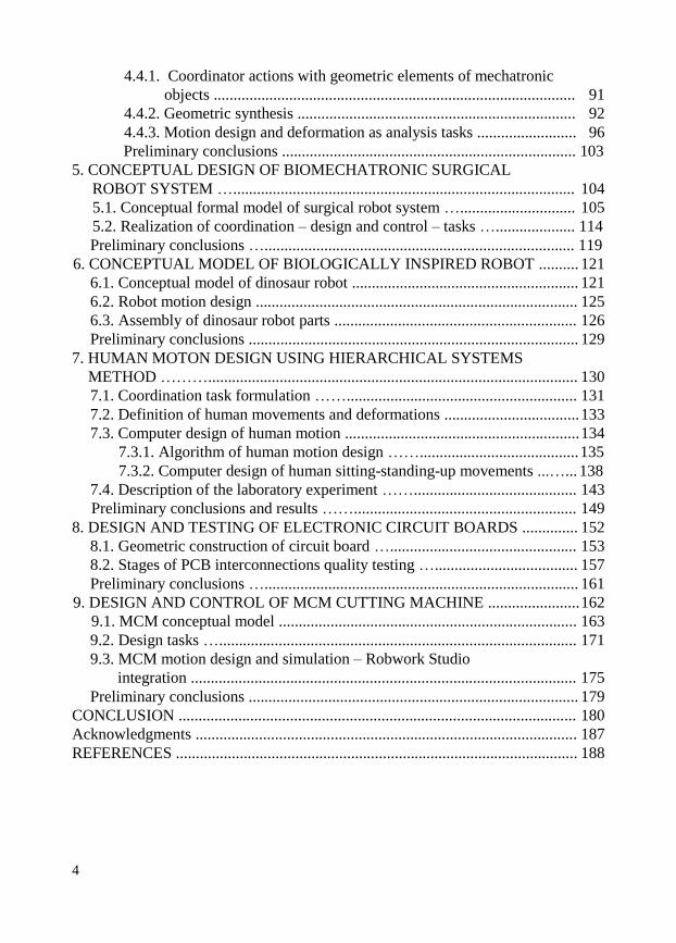
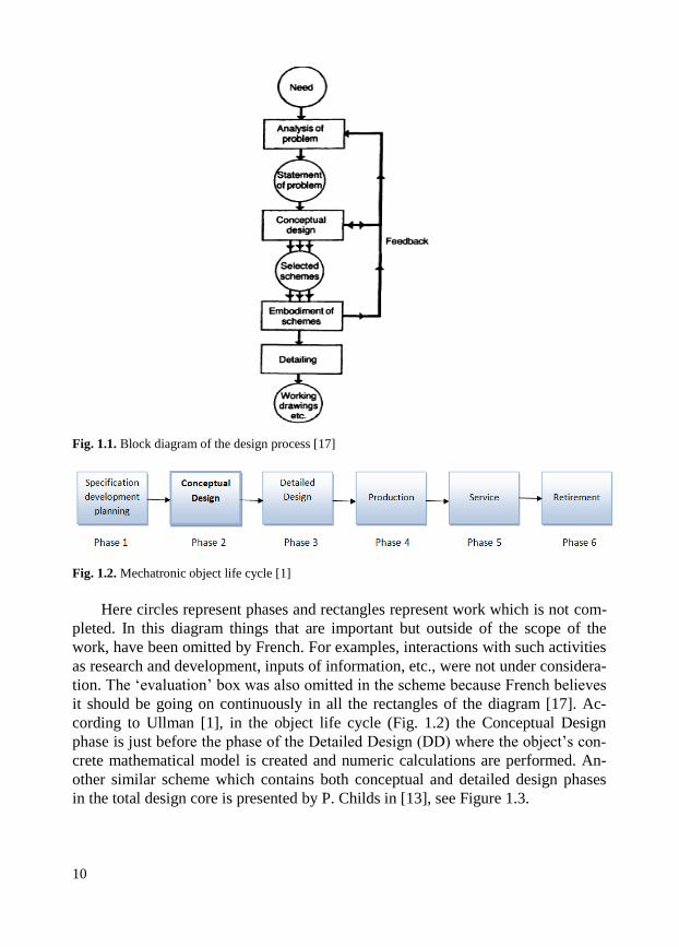
the form of a block diagram given in Figure 1.1.
10
Fig. 1.1. Block diagram of the design process [17]
Fig. 1.2. Mechatronic object life cycle [1]
Here circles represent phases and rectangles represent work which is not com-
pleted. In this diagram things that are important but outside of the scope of the
work, have been omitted by French. For examples, interactions with such activities
as research and development, inputs of information, etc., were not under considera-
tion. The ‘evaluation’ box was also omitted in the scheme because French believes
it should be going on continuously in all the rectangles of the diagram [17]. Ac-
cording to Ullman [1], in the object life cycle (Fig. 1.2) the Conceptual Design
phase is just before the phase of the Detailed Design (DD) where the object’s con-
crete mathematical model is created and numeric calculations are performed. An-
other similar scheme which contains both conceptual and detailed design phases
in the total design core is presented by P. Childs in [13], see Figure 1.3.

11
Fig. 1.3. The total design core [13]
The main design tasks performed at both CD and DD phases (Fig. 1.3) are
synthesis and analysis tasks. The places of these tasks in the general design process
are presented by the scheme in Figure 1.4 given in [13]. Synthesis is defined by
Childs as the process of combining the ideas developed into a form or concept,
which offers a potential solution to the design requirement. Analysis task is recog-
nized as involvement of the application of engineering science. In this case, sub-
jects are explored extensively in traditional engineering courses, such as statics and
dynamics, mechanics of materials, fluid flow and heat transfer. These engineering
'tools' and techniques are used in analysis tasks to examine the design to give quan-
titative information such as whether it is strong enough or will operate at an ac-
ceptable temperature [13]. Analysis and synthesis invariably go together.
In the frames of the conceptual design model presented in this book and de-
scribed below in aed formal basis of HS (see Chapters 3-4), the synthesis and anal-
ysis tasks are also performed together and defined as coordinator tasks of creating
(synthesis) and changing (after analysis) mechatronic system construction and
technology by selecting units of lower levels and settling their interactions to make

12
the state and activity of the system on higher levels (environment) best coordinated
with environmental aims.
Fig. 1.4. Synthesis and analysis design steps in the general design process [13]
Another definition of the conceptual design process was given in the Over-
view section of the work titled “Analyzing Requirements and Defining Mi-
crosoft.net Solution Architectures” [18] where MSF (Microsoft Solutions Frame-
work) process model was presented. It was pointed out here that the planning phase
of the Model involves three design processes: conceptual, logical, and physical.
The conceptual design starts during the envisioning phase of the MSF process
model and continues throughout the planning phase. Because the MSF design pro-
cess is evolutionary as well as iterative, conceptual design serves as the foundation
for both logical and physical design. The following three steps of conceptual de-
sign and associated baselines are formulated. Conceptual design is an iterative
process and the steps are repeated as required: 1) research, 2) analysis, 3) optimiza-

13
tion. The optimization baseline leads to the baseline of the conceptual design. Cor-
respondent Figure 1.5 illustrates these steps in the conceptual design.
During the research step of conceptual design, the team gathers more infor-
mation to refine and validate data collected during the envisioning phase. Typical-
ly, the information gathered during the envisioning phase is high level and lacking
in detail. During the first step of the conceptual design, the design team needs
to collect detailed information. For example, the team first identifies questions
raised by the first iteration of information gathering; the team then continues
to clarify the tasks, business processes, and workflow. As greater detail is discov-
ered, the results are incorporated in the use cases and draft requirements.
Fig. 1.5. Steps in conceptual design [18]
US Department of Transportation [19] formulated that conceptual studies (CS)
are typically initiated as needed to support the design planning and programming
process. CS phase identifies, defines and considers sufficient courses of action (i.e.,
engineering concepts) to address the design needs and deficiencies initially identi-
fied during the planning process. This phase advances a project proposed in the
program to a point where it is sufficiently described, defined and scoped to enable
the preliminary design and technical engineering activities to begin. The CS and
preliminary design phases are performed in conjunction and concurrently with the
environmental process which evaluates environmental impacts of the engineering
proposals resulting from the conceptual studies and preliminary design phases.
Environmental systems and processes are also taken into account in
knowledge based engineering (KBE) approach proposed by Pokojski and
Szustakiewicz in [20]. The main structures for extended KBE application are de-
sign process and design models. The models contain specific aspects such as prod-
uct structure as a whole and its fragments, engineering calculations and analysis
with ability of integration with external systems, design requirements and decision
making processes. This object-oriented approach makes it possible to speed up the
14
process of generating the source code of design models from the extended KBE
application. KBE approach is also used in [132] to support multidisciplinary design
optimization. Another approach where the decision support tools in the domain of
conceptual design are sufficiently developed is model-driven engineering (MDE)
described in [21]. Here, a prototype software is presented that allows the user to
specify functional requirements for the designed buildings, and hierarchical graphs
and graph grammars serve as knowledge representation tool.
In systematic respect, designing is defined in [22] as the optimization of given
objectives within partly conflicting constraints. Requirements can be changed with
time, so that a particular solutions can be optimized for a particular circumstances
set. In organizational respect, design is recognized as a part of the product life
cycle. This cycle is trigged by a market need or a new idea. Life cycle starts with
product planning and ends with recycling or environmentally safe disposal. The
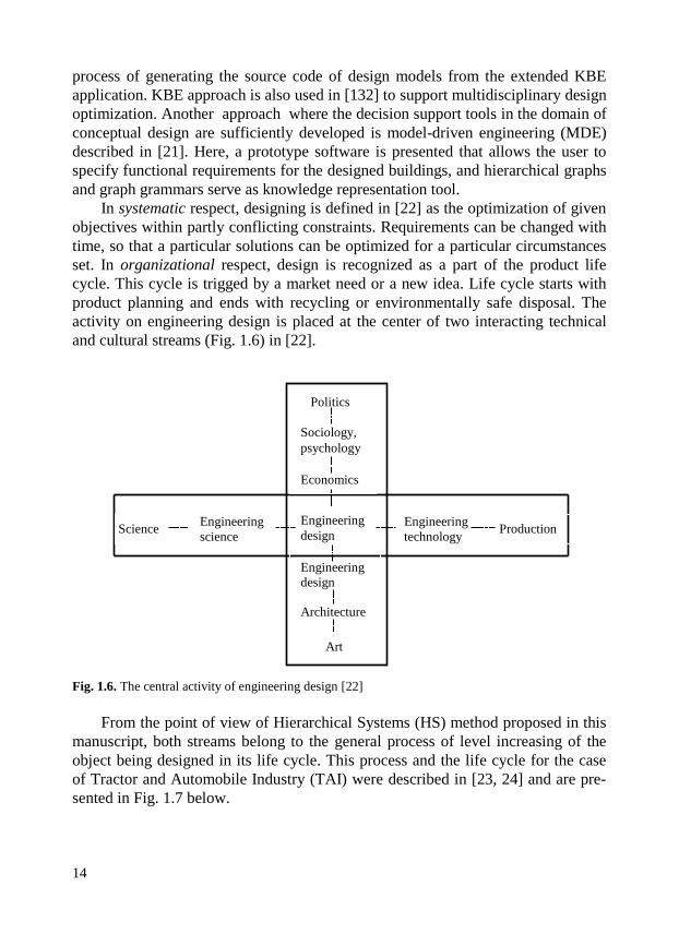
activity on engineering design is placed at the center of two interacting technical
and cultural streams (Fig. 1.6) in [22].
Fig. 1.6. The central activity of engineering design [22]
From the point of view of Hierarchical Systems (HS) method proposed in this
manuscript, both streams belong to the general process of level increasing of the
object being designed in its life cycle. This process and the life cycle for the case
of Tractor and Automobile Industry (TAI) were described in [23, 24] and are pre-
sented in Fig. 1.7 below.
Politics
Sociology,
psychology
Economics
Engineering
design
Engineering
design
Architecture
Art
Engineering
science Engineering
technology Science Production
15
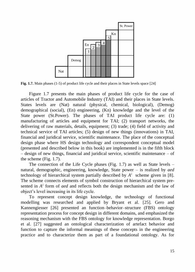
Fig. 1.7. Main phases (1-5) of product life cycle and their places in State levels space [24]
Figure 1.7 presents the main phases of product life cycle for the case of
articles of Tractor and Automobile Industry (TAI) and their places in State levels.
States levels are (Nat) natural (physical, chemical, biological), (Demog)
demographical (social), (En) engineering, (Kn) knowledge and the level of the
State power (St.Power). The phases of TAI product life cycle are: (1)
manufacturing of articles and equipment for TAI; (2) transport networks, the
delivering of raw materials, details, equipment; (3) trade; (4) field of activity and
technical service of TAI articles; (5) design of new things (innovations) in TAI,
financial and juridical service, scientific maintenance. The place of the conceptual
design phase where HS design technology and correspondent conceptual model
(presented and described below in this book) are implemented is in the fifth block
– design of new things, financial and juridical service, scientific maintenance – of
the scheme (Fig. 1.7).
The connection of the Life Cycle phases (Fig. 1.7) as well as State levels –
natural, demographic, engineering, knowledge, State power – is realized by aed
technology of hierarchical system partially described by Aλ scheme given in [8].
The scheme connects elements of symbol construction of hierarchical system pre-
sented in Aλ form of aed and reflects both the design mechanism and the law of
object’s level increasing in its life cycle.
To represent concept design knowledge, the technology of functional
modelling was researched and applied by Bryant et al. [25]. Gero and
Kannengiesser [26] presented an function–behavior–structure (FBS) ontology
representation process for concept design in different domains, and emphasized the
reasoning mechanism with the FBS ontology for knowledge representation. Borgo
et al. [27] suggested an ontological characterization of artefact behavior and
function to capture the informal meanings of these concepts in the engineering
practice and to characterize them as part of a foundational ontology. As for
Nat
Demog
En
g
Kn
St. Power
1 2
3 4
5

16
a mechatronic design process, Yan and Zante stated that "mechatronic system de-
sign is normally considered to be a sequential process in which a design solution to
a given design problem is generated, explored and evaluated following a series of
prescribed steps" [28]. A mechatronic approach towards designing inspection
robots using rapid prototyping and real-time simulation is also described by
Giergiel et al. in [29].
The design methods based on the abstract modelling of PALMERA and the
DMC model, Design Flow for Reconfigurable Architectures (INDRA) has been
developed to guide the designer through different implementation steps to create
a concrete dynamic reconfigurable system architecture. These design methods and
the design flow are described in [133, 134].
A formal definition of the concept design and a conceptual model linking con-
cepts related to design projects are presented by Ralph P. and Wand Y. [30]. Their
definition of design incorporates seven elements: agent, object, environment, goals,
primitives, requirements and constraints. The design project conceptual model
is based here on the view that projects are temporal trajectories of work systems
that include human agents who work to design systems for stakeholders, and use
resources and tools to accomplish this task. Ralph and Wand demonstrate how
these two conceptualizations can be useful by showing that 1) the definition of
design can be used to classify design knowledge, and 2) the conceptual model can
be used to classify design approaches. The analysis performed by Ralph and Wand
[30] led to defining the design as follows in Fig. 1.8.
Fig. 1.8. Conceptual model of Design as a noun [30]
Here the conceptual model of Design presented as a noun in Fig. 1.8 is recog-
nized as a specification of an object, manifested by an agent, intended to accom-
plish goals in a particular environment using a set of primitive components, satisfy-
ing a set of requirements, subject to constraints. The Design recognized as a verb is
presented to create a design in an environment where the designer operates.

17
Both noun and verb design definitions correspond to the object and its process
respectively as the elements of aed model of HS conceptual design method sug-
gested in this book, see aed scheme in Fig. 3.1, Chapter 3.
A systematic approach for the competency-oriented development of learning
factories integrating the conceptual design levels ‘learning factory’, ‘teaching
module’ and ‘learning situation’ is given by Tisch et al. in [129]. The presented
approach enables “an effective competency development in learning factories by
addressing problems of intuitively designed learning systems. As a result learning
factories, teaching modules and single teaching–learning situations meeting indus-
tries’ requirements can be realized with less effort and an increased success in ap-
plied competencies in real situations”. A systematic analysis of mechatronic ob-
jects is also presented by Gawrysiak in [104].
The function–cell–behaviour–structure (FCBS) model for better comprehend-
ing representation and reuse of design knowledge in conceptual design was pre-
sented by Gu et al. [31]. Hierarchical two-layer concept is given here, i.e. two
knowledge representing layers – the principle layer and the physical layer – are
presented in the FCBS model. The principle layer is utilized here to represent the
principle knowledge. Case modelling is employed in the physical layer to integrate
the structural information and behavioural performances of the existing devices,
which applies the design principles represented by the functional knowledge cells
(FKCs).
FCBS model presented by Gu et al. [31] and a formal definition of the concept
design and a conceptual model given by Ralph P. and Wand Y. [30] are close to
Hierarchical Systems design technology which is described below in this book and
was chosen in this work as the formal basis of the conceptual model creation.
In the presented book the Conceptual Design (CD) is recognized as a process
of creation of a systemic model of the object being designed on the early phase of
its life cycle. To define the conceptual model of a mechatronic system in systemic
bases it is necessary to describe: mechatronic system structure; its dynamic
representation as a unit in its environment; the system environment, its process
and system-environment interactions; the system coordinator and its coordination
(design&control) processes; processes executed by mechatronic subsystems and a
general process. Besides, the conceptual model should take into account the con-
nected descriptions of mechatronic subsystems of different nature, i.e. mechanical,
electromechanical, electronic and computer.
Furthermore, conceptual model of the mechatronic system being designed and
its coordination (deisgn&control) technology should meet the requirements of the
general design system which must allow performing the design – synthesis and
analysis – and control tasks under condition of any information uncertainty, i.e. (1)
to create and change mechatronic system construction and technology by selecting
units of lower levels and settling their interactions to make the state and activity of

18
the system in higher levels (environment) best coordinated with environmental
aims (selection stratum); (2) to change the ways (strategies) of the design task
performing when the designed unit is multiplied and the knowledge uncertainty is
removed (learning stratum); (3) to change the above mentioned strata when new
knowledge is created (self-organization stratum).
The coordination technology must also cohere with traditional forms of infor-
mation representation in mechatronics, i.e. numerical and geometrical systems. The
theoretical basis of the design process in agreement with these requirements must
be a hierarchical construction connecting any level unit with its lower and higher
levels.
The above mentioned methods used in the conceptual design and well as mod-
els of mathematics based on set theory and methods of artificial intelligence do not
meet the above formulated requirement. They do not allow the description of
mechatronic subsystems with their specific characteristic features in common
formal basis. At the same time they do not describe the mechanism of interlevel
dynamics of the mechatronic object (MO) being designed since the set theory de-
scribes one-level world outlook only.
To solve the problem, the symbol construction and coordination technology of
Hierarchical Systems (HSs) [2-8] was chosen in the work as the formal basis of the
conceptual model creation. HS formal model was constructed with the help of aed
(Fig. 3.1) – formal analogue of two-level system [3-8], and general dynamic sys-
tems by Mesarovic and Takahara [9,10], numeric positional system codes, geome-
try and cybernetics methods [32].
Among the first attempts of HS technology and aed model application in de-
sign are the results presented in [3-4, 33]. The current version of the conceptual
model and design technology of mechatronic objects based on the Hierarchical
Systems approach is partially described in [49] and presented below in this book.
19
2. GEOMETRIC MODELS IN DESIGN SYSTEMS
Geometric models of modern CAD systems which are used for solving the prob-
lems of mechatronics, robotics and automation are overviewed and analyzed in this
Chapter. The overview covers recent decades, when almost all theoretical geomet-
ric models were realized in design systems and some new ideas were formulated.
The main attention is paid to the models implemented in the systems which have
their commercial realization.
There are two main classes of geometric representations in computer aided de-
sign (CAD) systems and other automated systems – Boundary Representation, B-R
[34] and Constructive Solid Geometry, CSG [35].
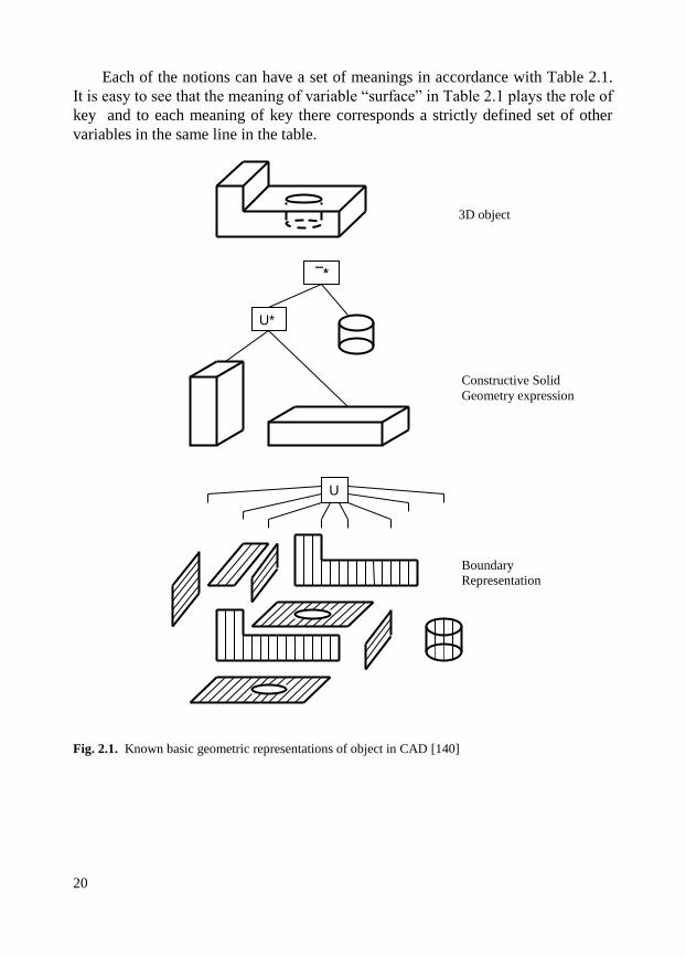
An object being constructed is presented by expressions of CSG type in the
form of a group of connected elementary objects (primitives) – cylinders, prisms,
spheres, cones etc. The connection can be formally described by algebraic sum, i.e.
some objects take part in this group with negative signs. CSG expression is graph-
ically presented as a tree, whose root is the whole object. The object unites the
details at each level, where the terminal tops (leaves) are primitives (Fig. 2.1).
Objects in B-R are represented by the set of parts of surfaces (sides) and the con-
nections between the sides by their boundaries (edges) may be indicated (Fig. 2.1).
It is easy to see that B-R in this case contains the set of boundary elements of
primitives which are used for uniting in CSG representation. At the same time, B-R
contains only such boundary elements which are connected with the environment
directly, and are not connected with each other in the whole object construction.
Therefore, after defining each primitive in CSG model by its boundary representa-
tion and erasing common parts of their boundaries we obtain B-R of the whole
object. It means that there is a simple transition from CSG to B-R but the reverse
process is not so simple.
Primitives and more complex objects can be presented in algebraic form, which
include patent, parametric [36], polynomial representations [37] and different types of
splines [37, 38], and also in the form of sequences of Euler operators [39]. Geometric
representation and parametric model of the object were proposed in the mid 80s of the
20th century. For geometric representation [40] the set of notions is introduced:
{surface, point, vectors, scalars} .
20
Each of the notions can have a set of meanings in accordance with Table 2.1.
It is easy to see that the meaning of variable “surface” in Table 2.1 plays the role of
key and to each meaning of key there corresponds a strictly defined set of other
variables in the same line in the table.
Fig. 2.1. Known basic geometric representations of object in CAD [140]
¯*
U*
U
Constructive Solid
Geometry expression
Boundary
Representation
3D object

21
Table 2.1. Multitude of geometric characteristics meanings
Surfaces Points Vectors Scalars
Plane Any point
on the plane
Unitary
normal No
Sphere Center No Radius
Rectilinear
cycle cylinder
Any point on the
axis
Unitary vector
parallel to axis
Radius, length
of axis
Rectilinear
cycle cone Top
Unitary vector
parallel to axis
Top angle,
radius
There is a certain mutual concordance between the representation of primitive
in the space of geometric characteristics and its algebraic definition in form:
Ax2 +By2 +Cz2 +Dxy+Eyz+Fxz+Gx+Hy+Jy+K=0, (2.1)
where: x, y, z are coordinates in 3-dimension Euclidean space. That means that
there are algorithms for transformation of geometric representation to algebraic one
and vice versa. Calculations presented in [40] show that geometric representations
require the minimal computer memory in comparison with other forms of represen-
tation. Besides, it is well connected with the natural language, convenient for en-
quiring about searching for elements of the object and forming directives for its
change. It is sometimes useful to calculate some metrical characteristics, such as
volumes and squares of surfaces using geometric representation directly. But it is
necessary to convert the geometric representation to other forms to calculate physi-
cal characteristics, to form graphic images and to determine the technological pro-
cess.
Objects and their primitives can be presented by the sequences of Euler opera-
tors [39]. Therefore, objects are described by the sequence of constructing opera-
tors and inverse sets of destructing operators of geometric objects of a higher (in
the case of destruction – lower) dimension. For instance, if we have an image of
polyhedron we can erase one of its apexes (vertex) and save this operation on com-
puter. After that we can erase another top which is located on the same edge. These
two operations correspond to the operation of the edge erasing. The sequence of
operations of erasing of all edges which form one polyhedron side corresponds to
the operation of removal of the whole side and finally, the erasing of all the sides
destroys the object.
The repetition of the chain of all the operations in the inverse sequence when
destructing operations are changed by constructing ones allows the object to be
rebuilt. Such direct and inverse chains are called Euler operators. Their name arose
from Euler’s formula:

22
v–e+f=2, (2.2) (2.2)
where: v – number of apexes, e – number of edges, f – number of sides.
Euler’s formula allows correctness of the object construction to be controlled.
General formula which corresponds to the object of any connectivity is presented
in the form of the expression:
v–e+f=2(s–h)+r, (2.3)
where: s – general number of untied components, h – number of through holes in
object, r – general number of cavities in sides.
For the formation of graphic images Euler operators are one of the best ex-
pressions. At the same time their most effective application to computer raster ter-
minal units is achieved by the hybrid connection of Euler operators with Octrees
[41]. Such trees finally include the white and black leaves only (i.e. empty and
filled elements of the object corresponding to cube primitives) but initially and in
the middle state they have the grey leaves as well. Grey leaf corresponds to the
case when one primitive simultaneously contains empty and filled areas. It is de-
composed according to the general rule for each level till only black and white
leaves remain.
Octrees is the most acceptable geometric model for raster graphics. The transi-
tion from Euler operators to Octrees is one of the way of transition from vector
(which is most useful for the output of boundary expressions) to raster representa-
tion [42]. It is necessary to convert Euler operators to other forms in order to calcu-
late functional characteristics of objects and to define technological processes.
The algebraic representations of geometric objects are well investigated
[40, 43].
They are not practically used in requests to search the objects and are hard for
their formation with participation of the user. There are some possibilities of con-
nection of created in this way primitives in CAD systems with CSG representation.
But connection algorithms of objects of various forms are very complex and re-
quire a lot of computer memory and time for calculation.
At the same time such representations are suitable for computer graphics tasks
(in vector forms), for generation of some programs for automated production and
are the most effective for calculation of many functional characteristics in many
tasks of engineering analysis.
The most convenient way of forming an algebraic expression is the case when
one of the input units of a computer is scanning a physically realized (or simply
graphically written) object. In this case the unit forms a range of observations dur-
ing a definite period of time which is changed later by corresponding mathematical
definitions. It allows the information to be compressed and the initial range of ob-
servations to be restored when necessary.

23
Rational parametrical B-spline [38, 44, 45] gives the general form of any ob-
ject’s surface representation in homogeneous, i.e. descriptive, coordinates.
The spline is obtained from common parametric B-spline in the following
way. C(t) is polynomial B-spline curve in 3D Euclidian space, i.e.
n
i
iki PtBtC1
, )()( , (2.4)
where: Pi – 3-dimention control points, t – parameter, such as a t b & a, b are
fixed and 0 a b; B(t) – polynomial of variable t of k order (power k-1). Bi,n(t) –
basic functions defined by node vector kn
jjt
1 and a = t1 = t2 = ... = tk < +tk1 tk+2
... tn tn+1 = ... = tn+k = b.
The representation of C(t) in homogeneous (descriptive) space with fourth co-
ordinate hi has the following form:
n
i
iki
n
i
iiki
htB
PhtB
tC
1
,
1
,
)(
)(
)( , (2.5)
or
n
i
hiki
h PtBtC1
, )()( , (2.6)
where h
iP is a control point in 4D space.
The corresponding spline representation for surface is defined by the expression:
n
i
jilj
m
j
ki
n
i
ijilj
m
j
ki
htBsB
PhtBsB
tsS
1
,,
1
,
1
,,
1
,
)()(
)()(
),( . (2.7)
This approach allows good representation of both the objects which are usual-
ly described by manifest definition (cycles, cones, primitive cubes) and the objects
which are defined with the help of the parametrical polynomial forms (sculptural
surfaces) [45]. The exemplary 2D path generated based on p(x, y) points using
Spline interpolation algorithm is presented in Fig. 2.2. Spline interpolation is used
in this case to create the 3 degree polynomials for the set of measurement points of
the cutting path. Technological process of the pipe cutting along the predefined
path is realized by robot cutter or CNC machine in production environment [46].

24
First, 1D spline for x and y point is created independently. Then the 2D path is
generated as the composition of 1D x and 1D y splines. The set of measurement
points in this case is as follows: 0 0,4 0,5 0 0,4 0,5 0,4 0x= and
0,5 0,4 0 0,4 0,5 0,4 0 0,5y= , see Fig. 2.2.
Fig. 2.2. 2D path generated based on p(x, y) points using Spline interpolation algorithm
The manifest functions require more elementary actions and less computer memory
for representation of primitive surfaces and lines. But the use of one general expression
improves the characteristics of the system in general and allows the memory volumes
for programs location to be reduced, the speed of operations to be increased and the
dialogue with the engineer to be unified. At the same time the expenses of system
development, exploitation and the amount of documentation are reduced.
Fig. 2.3. Tetrahedron – an example of a wire-frame model
Vertex list Edge list
V1(0, 0, 0)
V2(1, 0, 0)
V3(0, 1, 0)
V4(0, 0, 1)
e1[V1, V2]
e2[V2, V3]
e3[V3, V1]
e4[V2, V4]
e5[V4, V3]
e6[V1, V4]
z
x
V3
V2
V1
V4
e6
e5
e4
e3
e2
e1
y

25
For the case of wireframe modeling [46], the model consists entirely of points,
lines, arcs and circles, conics, and curves. In 3D wireframe model, an object is not
recorded as a solid. Instead the vertices that define the boundary of the object, or
the intersections of the edges of the object boundary are recorded as a collection of
points and their connectivity (Fig. 2.3).
Wireframe models are most economical in term of time and memory require-
ments, easy to construct, used to model solid object and often used for previewing
objects in an interactive scenario. At the same time the models have the following
disadvantages. They do not allow for use of photo realistic rendering tools, have no
ability to determine computationally information on mass properties (e.g. volume,
mass, moment, etc.) and line of intersect between two faces of intersecting models
and do not guarantee that the model definition is correct, complete or manufactura-
ble.
To expand the potential possibilities of traditional boundary representation, the
connections of dimensions (length, squares, volumes, angles) are added to algebra-
ic expression in the process of forming the representation. It permits the process of
parametric construction with the use of geometry of variations to be realized.
Parametric model, or which is often used for the representation of objects in
data bases of design systems, is defined by set {T, D, O, V, R, C}, where: T – set of
topologies, D – set of possible dimensions, O – set of operations, V – set of varia-
bles, R – set of relations between V and T/O/D, C – set of restrictions of the mean-
ings of variables.
Any class of objects PS can be presented in these terms in the following form:
PS ={t, d, o, v, r, c}, (2.8)
tiT, diD, oiO, viV, riR, ciC.
It is possible to create B-R defining T and D only. To create CSG it is neces-
sary to define O.
Therefore, parametric model of the object contains not only traditional repre-
sentations (B-R in its most developed form based on geometry of variations) but
also the relations between different forms of representations. Declarative definition
of all the elements of set {T, D, O, V, R, C} ensure flexibility of the system, possi-
bility of its adaptation to different classes of objects and optimization of system
parameters in its functioning process (for instance, finding more effective opera-
tions, defining new relations, etc.).
Having many characteristic features of systems of artificial intelligence, para-
metric model has a drawback – its relatively weak formalization. Six elements
presented above are not strictly defined. That makes the creation of such models
very complicated for the user. In other words, sets of possible meanings (states)
of objects T, D, O, V, R, C are not defined. Possible connections of these states, i.e.

26
states of the whole system, and transition operations from one possible state to
another are not defined either.
A more theoretically grounded from the point of view of realization simplicity
is the approach (independent from technical realisation) of graphical standard de-
velopment proposed by CGS Associates [47].
This approach is based on the application of mathematical means of formal
system theory and algebra for the development of data bases. GSC Associates has
adapted its technology in its commercial software products. Some of these products
are Computer Graphics Metafile (CGM) generator used by Apple, and CGM inter-
preter used by Microsoft, Apple and Symantec [47].
Geometrical objects are considered in [47] as formal systems which have their
inputs, outputs, states and actions of state transitions. A set of the actions also con-
tains the ways of obtaining information about the object’s state (states recognition).
Definite data structure of a data base corresponds to the formal system – ab-
stract data type, which can be adapted to any concrete state (any data of this type)
and the set of state transition functions, i.e. operations which do not take the ele-
ments out the frames of the abstract type being considered. For instance, the struc-
ture of group of integer numbers is defined on computer by a cell organised for
representation of integer number as a positional number with a definite base and
actions of adding and subtraction.
The cell can be in any of its states (can contain one of integer numbers pre-
sented in the computer numeric format). Each of the mentioned operations with the
present number and some other number which goes to the cell input are performed
with the help of sequence of elementary operations (with bits) and forms the output
which is also an integer number, i.e. has the same abstract type.
Division operation does not belong to the group of integer numbers because it
can take the elements out of the frames of this abstract type (it is necessary to have
one additional cell for the division remainder). The fields of real and complex
numbers, logical data are also realized in computers in the form of abstract data
types.
With respect to geometric expressions, this approach means the representation
of a geometric object in the form of abstract data type with a set of operations of
states transition which do not take the elements out of the frames of this abstract
type. For instance, the data structure “segment” can be defined by a set of axioms,
limits and by the operations of motion on a straight line, rotation and change of
length. The operation of arbitrary uniting of two segments is not included in the
data structure “segment” because it can take elements out of the frames of this
abstract type. For instance, it is possible to obtain the broken line or “+”-like object
as a result of uniting two segments, i.e. lines.

27
Data structure of “segment” also contains the operations with it. The descrip-
tion of several connected data structures for vector computer graphics with similar
organization is presented in [47].
In this case the analogy of parametric model set T, D, O, V, R, C is a set of no-
tions of formal system theory which corresponds to the language of abstract data
types. That means that the notions and their relations from this set are not only
strictly defined and easy for programming but are realized in many cases as hard-
ware.
So, concluding the overview of traditional ways of geometric information rep-
resentations, it can be pointed out that the possibility of formal system theory and
abstract data types application for the construction of expressions of geometric
objects (models) opens new perspectives in CIM systems including robotics and
CAD.
Both the CSG and B-R have their own advantages and drawbacks. So, the
CSG models are simply constructed with the participation of a user. CSG model
also requires less computer memory, is better adapted for definition of technologi-
cal processes (for inst. assembling type) and for imitation of movements of object’s
details.
On the other hand, B-R models can actually be built without human participa-
tion, allow the sculptural surfaces to be constructed, allow variations methods to be
used, and are better adapted for calculation of technological processes of continu-
ous deformation and for aerodynamic and hydrodynamic calculations.
The connection of these two approaches is possible, but sub-process of geo-
metric constructions creating and changing for CSG differs in marked degree from
this sub-process for B-R.
In the existing CAD-systems these are principally different design technolo-
gies. Integration of these approaches in one system can be possible in the case of
existence of the general formal language which can contain both representations
and transition operations from one to another. It looks like the hierarchical and
general systems theory can give an opportunity to create such a formal language. In
this book, the hierarchical geometry model given in Chapter 4 is used in design
tasks of mechatronic objects. The exemplary design tasks where HS (aed) geomet-
ric model is used are presented is Sections 4.4.2 and 4.4.3, and Chapters 6-8.

28
3. THEORETICAL BASIS
OF THE DESIGN METHOD
3.1. Formal model of hierarchical mechatronic system
Theoretical means of the both conceptual and detailed design method, as was stat-
ed in Chapter 1, must present the mathematical apparatus for formal description
of the designed mechatronic system (MS) structure, its aggregated dynamic repre-
sentation as a unit in its environment and the environment model. All the descrip-
tions should be connected by the coordinator which performs the design&control
tasks on its selection, learning and self-organization strata. Furthermore, theoreti-
cal means of the proposed mechatronic design method should allow presentation
of the numerical and geometrical information in its formal basis and be coordinat-
ed with the main requirements to design systems which must:
– carry out the main design and control task for the systems of any level
under the conditions of any initial knowledge uncertainty, i.e. to create or to
change the system construction and technology, to make its activity in a higher
level system (environment) most coordinated with the desired environment states
on all its levels (selection task);
– change the ways (strategies) of fulfilment of the main design and control
when designed constructions and technologies are multiplied and knowledge
uncertainty is removed (learning task);
– change the selection and learning strata when new (higher level) knowledge
constructions and technologies have been created (self-organisation task).
Traditional one-level mathematic, artificial intelligence and cybernetic models
and methods used in conceptual and detailed design do not meet all the above men-
tioned requirements, because it is impossible to express interleave relations in their
terms.
Therefore, the construction of hierarchical system (HS) with its standard block
aed (formal analog of two-level system) has been chosen as the theoretical basis
for conceptual and detailed mechatronic design performing. Aed – ancient Greek

29
word – is a standard element of design systems [3-7, 33, 49], which realizes the
general laws of systems organization on each level and the inter-level connections.
The first version of aed model was described in [3-5, 33], and later in [6-8].
Aed contains all the characteristic features of two-level system [2] and also the
following ones:
1) for inter-level connections modeling aed contains more levels, the block of
environment , in particular;
2) two-level system in [2] is not sufficiently formalized for measuring quanti-
tative characteristics and for investigating dynamic laws of hierarchical systems;
aed formal model is based mainly on the two particular cases – dynamic
systems [9, 10] and numerical positional systems by H. Lebesque [48].
3) structural connections in two-level system were explored only for the meth-
od of the general systems synthesis [9, 10], but the nature and the dynamics of the
connections were not revealed;
connections in are hierarchical systems and can be described by aed
formal model; for structural connections and for the connections of system
with environment the laws of their coordinated dynamics, i.e. the dy-
namics of inter-level transition are defined;
4) the coordinator of two-level system does not change its own state; it is con-
nected only with the subsystems being coordinated and cannot construct or change
the formal model of two-level system;
coordinator 0S of aed is constructed from the interactions of lower level sys-
tems coordinated and directly connected with the coordinator 10S of higher level.
The dynamics of 0S states was explored for four periods of time: , ,
and ( , , , , – time of level ). The initial moment
for each concrete system and its coordinator 0S is the moment
Tt 0 .
Moment t is fixed when the elements
S of level )( of system
have arisen. For time the formal model TS | allows the experimental check-
ing of its coherence only with the systems of lower levels ~
)0(
and cannot be coordinated with the synthesis laws of level systems. It causes
improvement of the model. During the process of system synthesis its coordi-
S
S
S
, S
S SS
S S
T
T
T
T
TT
T T
T T
S
S
T
S
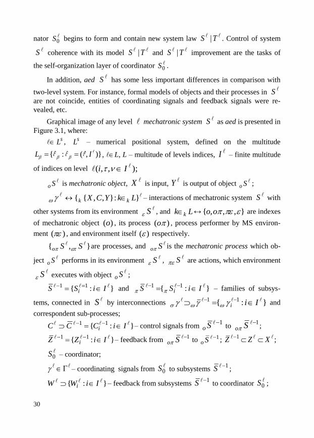
30
nator 0S begins to form and contain new system law
TS | . Control of system
coherence with its model TS | and
TS | improvement are the tasks of
the self-organization layer of coordinator 0S .
In addition, aed has some less important differences in comparison with
two-level system. For instance, formal models of objects and their processes in
are not coincide, entities of coordinating signals and feedback signals were re-
vealed, etc.
Graphical image of any level mechatronic system as aed is presented in
Figure 3.1, where:
sL , sL – numerical positional system, defined on the multitude
{ : ( , )}L I , L, L – multitude of levels indices, I – finite multitude
of indices on level
So is mechatronic object, X is input,
Y is output of object So ;
– interactions of mechatronic system with
other systems from its environment , and ↔ are indexes
of mechatronic object , its process , process performer by MS environ-
ment , and environment itself respectively.
are processes, and is the mechatronic process which ob-
ject So performs in its environment , are actions, which environment
executes with object So ;
}:{ 11 IiSS i and – families of subsys-
tems, connected in by interconnections and
correspondent sub-processes;
}:{ 11 IiCCC i – control signals from 1So to ;
}:{ 11 IiZZ i – feedback from to 1So ; ;1 XZZ
0S – coordinator;
– coordinating signals from 0S to subsystems
1S ;
}:{ IiWW i – feedback from subsystems 1S to coordinator
0S ;
S
SS
S
);,,( Ii
}:},,{{ LkYCX kk
S
S Lk k },,,{ oo
)(o )( o
)( )(
},{ SSo So
SS
S
1S }:{ 1 IiSi
S }:{ 11 Iii
1So
1So

31
– coordinating signals for system S ;
– feedback from 0S to coordinator
10S of higher level.
Aed S is a system which has the following characteristic features:
– environment contains a set of systems of level ;
– it is possible to present S as object So , its interactions with cre-
ate a higher level system;
– process contains both the actions which the object So per-
forms in environment and actions of environment system
with object So ;
– dynamic realization of S in is defined by aggregated model
, , where and
are aggregated dynamic models of object So , environment
and their processes , respectively;
– structure contains the lower level systems 1S with their interac-
tions which create coordinator 0S and in this way connect
with :
}~,{ 0 S , ;
– the task of coordinator 0S is to create not only systems
S but also
(partly) higher levels systems; for solving this task coordinator 0S constructs
the informational models of concrete systems )( LS ; the models are con-
structed from the elements of interconnections of S with other systems
S of
level ℓ and must be coordinated both with S and higher levels systems;
– incoherence of the models with concrete systems causes a change of the
abstract informational model of S by coordinator
0S .
Definition 3.1. Mechatronic system S is expressed by the next aed formal
system:
, (3.1)
X 1
YWw 1
S LS
SSo
SS
S
S
},~{ 0S }},,{},,{{~ oo ,o
,oS
SoS
~ }},:}:{{{ s
i LIi
S }, { 0 S
32
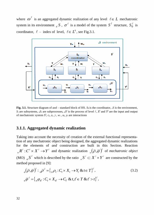
where is an aggregated dynamic realization of any level mechatronic
system in its environment S , is a model of the system S structure, is
coordinator, – index of level, , see Fig.3.1.
Fig. 3.1. Structure diagram of aed – standard block of HS. S0 is the coordinator, εS is the environment,
Si are subsystems, πSi are subprocesses, πSl is the process of level , Xl and Yl are the input and output
of mechatronic system Sl; ci, zi, , wi , ui, yi are interactions
3.1.1. Aggregated dynamic realization
Taking into account the necessity of creation of the external functional representa-
tion of any mechatronic object being designed, the aggregated dynamic realizations
for the elements of aed construction are built in this Section. Reaction
and dynamic realization of mechatronic object
(MO) which is described by the ratio are constructed by the
method proposed in [9]:
, (3.2)
,
L
0S
sL
YXСRo : ,o
So YXS
o
TtYXC ttttooo &::,
ttTttCXC ttttttoo &,&:

33
where is the time of level , reaction ρ, state transition function φ, and time
interval tt’.
Model of actions, i.e. processes which object performs in envi-
ronment changing its own state differs from the model
of the object:
– object of initial states of process coincides with the object of
inputs ;
– input of process is defined by states , their altera-
tions are control signals to process .
Taking into account the differences, dynamic realization of mecha-
tronic process connected with is presented in the following way:
, (3.3)
.
The expression for shows that the input of object is defined
not only by the environment but also (partially) by system in process
, i.e. can form its inputs by itself.
Actions of environment system with the object are also
formalized by dynamic system :
, (3.4)
,
where is both the state of environment and inputs of process ;
is the state of environment process , tt’ is a time interval.
Aggregated dynamic models of actions of systems
and are defined as :
T
SoSo
S Cс
,o
CSo
XX
So Cс
So
,o
So ,o
TtYCX ttttooo &::,
ttTttXCX ttttttoo &,&:
,oSo
SS
SoS
SS
So
,
TtXCY tttt &::,
ttTttYCY tttttt &,&:
СS
S
tY S
},{ SSS o
SoS ,

34
={ , }. (3.5)
The model of environment of system is presented as follows:
, (3.6)
.
The coherence condition of constructed models with concrete mechatronic
systems were regarded. As stated in [9], for reaction family
coherence with the time system it
is necessary and enough the execution of the following conditions [9]:
, (3.7)
.
Time system is called a dynamic system only when it is possible to find both
the reaction family and the family of the state transitions coordinated with
the system, and all functions satisfy the conditions (i)–(iii) [9]:
(i) (3.8)
(ii)
(iii)
The coherence conditions similar to and (3.7) for the object reac-
tion are presented in the following way:
,(3.9)
.
The conditions for , , are constructed similarly taking into
account the meanings of states, inputs and outputs in the dynamic representations
of processes , and environment (3.3-3.6). The meanings are
, ,o ,
SS
TtYXC tttt &::,
ttTttCXC tttttt &,&:
TtYXC tttt &: YXS
)1( ]),(),()[)()()(( 000 tt
t
ttttt
t Txxcxccxxc
)2( ]),(),()[)()()(( 000 tt
t
ttt
t
tt Txxcxcxcxc
tt
),),,((),( ttttttttttt xxcTxc ;tttt xxx
),),,((),( tttttttttttttt xxcxc ;tttttt xxx
.),( tttttt cxc
)1( )2(
o
)1( o ]),(),()[)()()(( 000 tt
totttott
t Txxcxccxxc
)2( o ]),(),()[)()()(( 000 tt
tottto
ttt Txxcxcxcxc
o
SoS
S

35
presented in Table 3.1, where and are parts of and im-
mediately not dependant on .
Reaction families , , , are coordinated with ,
, and only when corresponding conditions ( ,1o )2o ,
, and , which are called coherence
conditions of and , are realized.
Conditions (i)-(iii) (3.8) for function of states transition are presented as
follows:
o(i) , (3.10)
o(ii)
o(iii) .
Table 3.1. Connections of states, inputs and outputs for , , and
The conditions for , , are constructed similarly taking into
account the meanings of states, inputs and outputs (Tab. 3.1) in the dynamic repre-
sentations of , and (3.3-3.6).
So, the following qualities of the model being created and correspondent defi-
nition were formulated. If the coherence conditions of with and conditions
XY
XY
S
o
o
So
SoS
S
1( o )2, o ,1( )2 ,1( )2 S
o
)),,((),( '''''
ttttttototttto xxcTxc
;''
tttt xxx
),),,((),( '"""'"''
tttttttottottttto xxcxc
;'""'
tttttt
xxx
tttttto cxc ),(
So
SoS
S
C X Y
SoC X Y
SoX C Y
S XYX C
YXY
SC
XYX YXY
o
SoS
S
S

36
o((i)-(iii)) –((i)-(iii)) are realized, systems , , and
are dynamic.
Definition 3.2. Set of dynamic systems { , , } con-
nected by connections and the creating system (coordinator) are called
dynamic realization of hierarchical system of any level :
{ , } { , } . (3.11)
Where is presented in the following form:
(3.12)
,
and is as follows: ,
Thanks to the strong connections of components through their inputs,
outputs and states, the ability of reconstructing from its parts as well as calcu-
lating unknown parts from its known ones was obtained.
The following relations are revealed. Process bonds the
systems and . Dynamic realization ={ ,
} as well as are the relations of models and
in . The difference of and models (similar to
and ) is caused by the fact that the processes, i.e. actions, have their own
sense in the coordination tasks described below.
With regard to the constructed dynamic realization of the system being de-
signed, the main three tasks, which coordinator performs in are singled
out:
on selection layer receives the coordination signals from higher lev-
el and forms feedback signals by the way which takes into account the run-
ning level of information uncertainty in model;
,o ,o ,
,
,o , ,
0S
L
}},,{},,{{ oo
0S
~ 0S
~
~ }},,{},,{{ oo
}}0,:{,,{{ 0
sL }},:{{ sL
kk ),( k Lk k }.,,,{ oo
~
},{ SSS o
SoS , ,o
, ,o ,
~ ,o ,o ,
,
0S
0S 1
1w

37
on learning layer adapts models to concrete system and makes
concrete the parameters of abstract system components (removes the uncer-
tainty);
on self-organization layer can change model and both ways of its ad-
aptation to concrete systems and feedback signal forming, i.e. the ways of
solving the tasks of choice and learning layers.
Models , and are constructed from the infor-
mation about interactions of system with environment and can be
obtained by coordinators , and , ( ). Therefore,
coordinator of each system of level can predict changes in system
and in part controls them, performing in this way the functions of coordinator
of higher level .
Aggregated dynamic realization of each system is constructed from
the elements of this system by the laws of level . On the other hand, is
formed from connecting elements of system with environment , i.e. from
the elements of other systems of level , and contains information about the indi-
vidual characteristics of these systems. Therefore, begins to reflect the general
laws of higher level systems and can, therefore, be regarded as a part of
coordinator . In this way coordinator is connected with and contin-
uous connection of discrete level is obtained.
3.1.2. Structure
The model of mechatronic system structure is introduced for the construction de-
scription of an object being designed. The structure is defined as follows.
Definition 3.3. The next formal system is called a structure :
{ 0S , }, (3.13)
0S
S~
0S
1w
,o , ,
S S
0S 1
0S
iS01 Ii
iS0S
0S 1S
10S 1
S
S S
1S1
0S
0S 10S
~

38
and is as follows:
,(3.14)
where:
0S is coordinator,
are aggregated dynamic models of subsystems,
, ,
are connections of the subsystems,
.
is the connection of dynamic systems and their interactions
coordinated with . The dynamics of structural intercon-
nections illustrates the dynamics of system organization from moment
.
Aggregated dynamic models are formed both by coordinators of
systems and coordinator of a higher level, i.e. are the interlevel
connections of coordinators and .
3.1.3. Coordinator
For the description of the design system and its functions in the design process the
model of coordinator is constructed in this section. The first version of the model
was initially described in [3] and later improved and presented in [4-8,49].
Coordinator is the main element of hierarchical systems which realizes the
processes of mechatronic systems design and control. It is defined in the following
form in accordance with aed representation (3.1).
~
~ }},:}:{{{
si LIi
}},:{{ 0 sL
}:{ IiSS isL
}:{ Iii
t
~
S
S
T0
1 10S
1S0S 1
0S 1
0S
0S

39
Definition 3.4. The following system is called a coordinator:
, (3.15)
where: is aggregated dynamic realization of ,
is the structure of ,
is coordinator control element.
That is has own aggregated dynamical realization and structure .
is defined recursively. Coordinator constructs its aggregated dynamic realiza-
tion and structure by itself. The development of coordinator formal model
on each level
goes from its initial state from moment
simultaneously with aed formal model develop-
ment for level .
Dynamic realization of coordinator is constructed from the infor-
mation about its interactions with coordinator environment :
= { , , }= , , (3.16)
where is input of , is output of , are structural connec-
tions of .
With this aim, the inputs, outputs, both structural and external
connections of coordinator were defined on the sets of its coordination signals
and feedbacks as follows:
={ , }, ={ , }, (3.17)
={ , , }= , { , , } = ,
0S
000 }, { SS
0
0S
0
0S
00S
0S 0 0
0S
0
0
L TS0
TTT tt 0
TS
0
0S
0
0S
0
0X
0
0Y
0
sL 0
0X
0S
0Y 0S
0
0S
0
0
G
W
0X 1G W
0Y G 1W
0
W G1
0
1G 1W1
0

40
where: – coordination signals for systems , – feedback from ,
– feedback from to coordinator of higher level, – coordi-
nation signals from to
.
The meanings of and were revealed. For each moment coor-
dination signals contain the forecast of meanings of structure pa-
rameters for period :
. (3.18)
Feedback signal transfers to coordinator the actual values of
all the parameters of structure as well as predictions of made by
the coordinators of systems of lower level:
= , . (3.19)
It is shown, that feedback contains the analogue of coordination signals
, i.e. each coordinator of lower level ℓ-1, being the part of coordinator
can fulfil its functions, as stated above.
Signals and of higher level were presented just as in
(3.16-3.17):
, = (3.20)
The availability of coordinator control element allows evaluation and
changing of coordinator by itself. Let:
, , , (3.21)
, , ... ,
.
G1S W 1S
1W 0S 1
0S 1G
10S
0S
wTt
Gt
tT
|{ t}tT
Ww t 0S
tT tT
1S
tw tT { 1} tT
w
10S
0S
1t
tw )1( 1
1111 }{ tt T t
w)1(
.},{ 11)1(1 t
t TT
00S
0S
??
...}?,,,,{ L

41
Then ; is contraction of system on the
and
, (3.22)
,
, ...
Systems are strata of coordinator and is the outlook in the level
space. Structure of coordinator is presented as a multi-strata hierarchical sys-
tem in agreement with [2]. Functions of each stratum are formulated as presented
below.
The main design task is performed on the selection stratum when the
strategies of (processes ) connect the structure dynamics and
with using . Coordinator produces actual values of coordination
signals , and receives feedback signals , on its selection
stratum. The ways of generation and receptions of signals (coordination strategies)
depend on coordinator state and state of its environment . For each
way there are several levels of information uncertainty and system organiza-
tion.
The information uncertainty of increases with the distance from . Every
level of uncertainty on every strata has its own coordination strategy.
The change of strategies is executed by learning layer (the moment it
can do it) and it is controlled by the following (self-organization) stratum. At
the same time the outlook in the level space extends from to
. Uncertainty removal in outlook is equivalent of system or-
ganization increasing (the increasing of interactions level), when realizations
are united and multiplied by , which realize the level increasing pro-
cess in hierarchic space .
LS &S 000
0S S
SSSS 0:
000 },{ S S
000 },{ S S
000 },{ S S
0S
0S
0S
0S
0S
0So
0S
1G G W 1W
0C
0C0S
S
0S
0S
0So
0S
0S
0S
0S
S )(
S

42
On the learning stratum coordinator changes the coordination strategies
removing in this way uncertainty and improving the organization level of system
. In case when the formal model of aed for level is known, the task
of uncertainty removing is reduced to the task of selection of a concrete variant of
the formal model which is used for generating signals , and receiving
information , .
Formal model is constructed on self-organization stratum of the
coordinator, i.e. this stratum can change the state of both learning and selection strata.
Therefore, the coordination strategies on selection stratum correspond to the
coordinator reactions for different states, and the functions of learning and
self-organization strata correspond to the functions of states transition.
Aggregated dynamic representation of coordinator is presented by
analogy with (3.11) as follows:
{ , } { , } . (3.23)
Where 0
~ is presented in the following form:
(3.24)
,
and is as follows: , Here
, ={ ,0),( } and are dynamic real-
izations of coordinating element , coordination process ={ ,
} which is decomposed into actions which element performs
in its environment and actions of with coordinating element
, and the coordinator environment respectively. Each component of the
dynamic representation (3.24) are described just as in (3.2-3.6):
, (3.25)
.
0S
S TS
G 1W
1G W
TS 0S
0S
0
0S
0 }},,{},,{{ 00000 oo
0S
0~
0S
0
~ }},,{},,{{ 00000 oo
}}0,:{,,{{ 000
0
sL }},:{{ 0 sL
0k
0k
0),( k Lk k }.,,,{ oo
0,o 0, 0,o 0,
0So
0S
0So
0S
0So
0So
0S
0S
0S
0So
0S
TtYXC tttt &::, 000000
ttTttCXC tttttto &,&: 00000

43
The connections of states, inputs and outputs of coordinating element ,
processes and coordinator environment are shown in Table 3.2.
Table 3.2. Connections of states, inputs and outputs of coordinating element , processes
and environment of coordinator
Dynamic realization of coordinator is defined on its structure which
contains a set of coordination strategies { } and their connections { }, i.e.
coordination subsystems in .
Coordination strategies are realized through the elements of coordinator sub-
systems of lower levels which are connected by . In
other words each strategy has its own structure which is improved in accordance
with the changes of the organization level of system and of the level of infor-
mation uncertainty of its coordinator .
Dynamic model is the initial stage of future investigation of coordinator
and is still not concrete enough.
The next step is the introduction of the states space structure on the objects of
initial states of model components and the transition to the canonical model of
the coordinator.
Canonical model :
{{ , ,0)ˆ,ˆ( }, } { , }, (3.26)
0So
0S
0S
0So
0S
0S
0
C X Y
0So
0C
0C 0Y
0So
0X
0C 0Y
0S
0Y
0C0X
0S
0C
0X
0Y
0
0
0
0
0,0S
0,,0 sLS 0
S
0S
0
0S
0
0
0
0)ˆ,ˆ( o0)ˆ,ˆ(
0S
0
~
0S

44
is constructed on the basis of multi-layer system conception [2], where functions
{
} correspond to learning and self-organization strata and functions { }
correspond to coordination strategies on selection stratum. The run of the process
of canonical model constructing is described below in Section 3.2.
3.2. Canonical model of coordinator
To describe the dynamics of both mechatronic object being designed and its design
system, the different states of system and its coordinator canonical model
are defined in this Section. The descriptions of the states are presented for different
moments of time, which correspond to the consequent stages of mechatronic sys-
tem creation and elimination of information uncertainty of its coordinator. For each
state of the system the most rational design and control strategies of coordinator
are formulated as presented below.
The initial moment of both system of level and its coordinator
arising is ( is time of level ), when at least one system
of level ( ) appeared. Index ψ corresponds to the low-
est organization of systems of level .
The initial period of and is the period of time ,
where is the moment, when the set of elements are united in system
of level , = +1.
For the moment of time
formal model of aed is defined by contraction and its con-
formity with concrete systems is approved experimentally for levels only;
concrete bearers of formal model are systems ;
0
0
S 0S
S 0S
Ttt 0T
S ,L
S
0S TTTtt
t
S S
:? TTt
STS
~
S S

45
synthesis laws of level system are unknown but can be defined by the ex-
trapolation ;
the form of representation of coordination signals and feedback sig-
nals is system ;
system is in the state of the weakest organization (the difference
between system level and level of its elements runs up to maximum);
coordinator is in the state of the highest uncertainty of information;
signals and should be regarded as undefined be-
cause system is unknown.
The most rational coordination strategy for such conditions is the coordination
of interactions when coordinator allows the systems to make a free
choice of concrete parameters of interactions and, consequently, any dy-
namic realizations of systems and its any allowed combinations .
From moment to ( , ) system achieves
the state of partial organization. Moment can be fixed when at least one system
of level
( ) reaches the state of complete organization. is
the moment when system ( ) has been formed.
For this period of time coordination strategy in is evaluation of in-
teractions. While realizing this strategy coordinator defines the coordination
signals for each new system of level by bounds of concrete values and
standards with the evaluation of belonging to this standard state. Coordination sig-
nals and feedback signals are formed in by the coordination of
interactions on level +1.
STS
Ww S
TS
TS0
11 11 Ww
1S
0S S
~ S
t
t
t
TTTttt
,
S
t
S
)1( t
S )1(
T
0S
1 1wT

46
For the moment ( , ) struc-
ture of system becomes sufficiently organized and is regarded as
system of level ( ).
For moment of time :
formal model goes to state of full certainty with laws of level of
synthesis of structures ;
concrete bearers of are systems ;
the synthesis laws of level systems become known, and the laws of their
functioning in are known with the accuracy of parameters concrete value;
the form of coordination signals and feedback signals representation
is determined system ;
it is possible to find the range of systems sufficiently organized by ;
coordination systems are in the state of minimal information uncertainty;
formal models of systems and are realized in states and
; models of systems and are in states and
accordingly; systems and have been formed.
Coordination strategy in structure in this case is interconnections prediction.
For the period of time , which begins from moment , the task of
changing is the task of higher levels.
Summarizing, it should be pointed out that on each level the formal
model is consecutively changed from state to states , ,
and the following quality is true:
t
TTTttt
,
TTTtt
S S
S )1( )3()2(
TT
S S
S S
1S
w
STS
S
0S
1S1
0S 1S
10S
2S 20S 2S
20S
3S3
0S
t
TT t
TS
LS S
SS
S
s

47
(3.27)
,
where symbol ψ means the lowest certainty (highest information uncertainty) of
the corresponding value, and symbol λ means the highest certainty.
Abstract system ={ , , , } of states of formal model
codes the multitude of ways of information representation on each level
and is the basis for canonical model of coordinator .
3.2.1. Presentation of coordinating element
Similar to aed dynamic realization (3.11), which was constructed for mechatronic
object, its process and object’s environment, the coordinator dynamic realization is
constructed for coordinating element – design system analogues, coordination pro-
cess and environment of coordinator. The process of the creating of canonic
presentation of coordinating element is described below.
The canonic representation is constructed on the external interactions of
coordinator. The external connections of coordinator depend on the or-
ganization level of mechatronic system and information uncertainty of its
coordinator .
First, the following mapping is marked by symbol as follows:
: . (3.28)
After that, the introduced equivalence relations :
( , ) ( )= ( ), (3.29)
make it possible to construct the following multitudes:
)( S
332211& TttTttTtttSTS
332211 && STSSTSSTS
sS
SS
S
S
L 0S
0
0
0S
S
0S
R
R0
0E
0
01
02 E R
01 R
02

48
={ , , , }, (3.30)
where , , and are equivalence classes of coordinator
connections by uncertainty levels of information.
Equivalence classes for coordinator states are introduced to con-
struct the state space of the coordinator.
Set and equivalence ratio are defined by the following expres-
sion :
(3.31)
.
Factor multitude { , , , } is called the
states space of coordinating element , where , , , are
the classes of states equivalence of by information uncertainty levels.
The state transition function in the introduced state space is defined by the
next expression:
(3.32)
where , and such
as:
(3.33)
where is an arbitrary element from state space , It is mapping.
E0
0
0
0
0
0
0
0
0
0S
tt Cc 00
Tt
tCC
00
~
0
~CEc
0
~C
ctt Ecc 021 ),(
))([( 00 xTt ))),((( 00010
to TxcR
&)])),((( 00020
to TxcR
))('[(& '0ttxtt ),,(( '010'0
ttttto xc ])),( '020'0 cttttto Exc
cECC 00
~ 0C
0C
0C
0C
0So
0C
0C
0C
0C
0So
0C
)~
(:ˆ 0'0 ctto EC ,)~
( 0'0 ctt ECX
)],([ˆ '00'0tttto xc )]]),([(ˆ[ '00'0
ttttto xcI
tct CECI 00
~:
*0tC
tC0
, ] [ &
] [ & ] ([
0 0 0 *
0
0 0 0 0 0
t t t
t t t t
C c C c
C c c c c I

49
The composition conditions (i)-(iii) for function are presented similar-
ly as for conditions (3.10) for function .
The output function for states space is presented in the following form:
(3.34)
where: is input alphabet; is output alphabet of , and the following
quality is true:
. (3.35)
Fig. 3.2. Commutative diagram of output and state transition functions
From the execution of the last equation (3.35) and conditions (i)-(iii) for func-
tion it is presumed that the diagram in Figure 3.2 is commutative, and the
following system:
, (3.36)
,
'0ˆ tto
o
0C
)~
(:ˆ00 cto EC ,
~~00 YX
0
~X
0
~Y
0S
)~],([ˆ000 xcto )]]),([([ '000
tttto xcI
I
'00 ttXC
'00 ttt XC
})'{,ˆ( '0 tRtto })'{,( *
'0 tRtto
I
00
~XC
'00 ttXC
'0
ˆto
'0to
0
~Y
'0to
'0ˆ tto
'0ˆ tto
0'00'0 :ˆ CXC tttto
0000
~~:ˆ YXCto
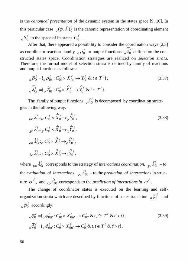
50
is the canonical presentation of the dynamic system in the states space [9, 10]. In
this particular case is the canonic representation of coordinating element
in the space of its states .
After that, there appeared a possibility to consider the coordination ways [2,3]
as coordinator reaction family or output functions defined on the con-
structed states space. Coordination strategies are realized on selection strata.
Therefore, the formal model of selection strata is defined by family of reactions
and output functions as follows:
, (3.37)
.
The family of output functions is decomposed by coordination strate-
gies in the following way:
, (3.38)
,
,
,
where corresponds to the strategy of interactions coordination, – to
the evaluation of interactions, – to the prediction of interactions in struc-
ture , and corresponds to the prediction of interactions in .
The change of coordinator states is executed on the learning and self-
organization strata which are described by functions of states transition and
accordingly:
, (3.39)
.
0)ˆ,ˆ( o
0So
0C
0o
0o
}&:{ 00000 TtYXC ttttoo
}&~~
:ˆ{ˆ00000
TtYXCtoto
0o
0000
~~:ˆ YXCto
0000
~~:ˆ YXCto
0000
~~:ˆ YXCto
0000
~~:ˆ YXCto
to 0
to 0
to 0
to 0
0o
0o
}'&',&:{ '0'00'00 ttTttCXC ttttttoo
}'&',&:ˆ{ˆ 0'00'00 ttTttCXC ttttoo

51
Function is decomposed into two functions – and , where
performs states transition on the learning stratum, and – on the self-
organization stratum. So, only changes of coordination strategies are possible on
the learning stratum. The form of their representation is fixed. On the self-
organization stratum the forms of information representation and processing
ways can be changed.
3.2.2. Process of coordination
Dynamic realization of coordination process is decomposed into
the model of process which the coordinating element performs in envi-
ronment and model of process by which constructs :
={ , }. (3.40)
,
.
,
,
where = { , } and ={ , }. and
are com-
ponents of inputs and outputs of coordinator environment which are con-
trolled by coordinator only in part.
Each of the above models is also decomposed into two ones. Dynamic realiza-
tion is decomposed into the processes in and and
into the processes of coordinator construction from lower (from )
and from higher (from ) levels:
0o
0o
0o
0o
0o
0,0So
0,o
0S 0,
0S
0So
0, 0,o 0,
TtYCX ttttooo &::, 000000
ttTttXCX ttttttoo &,&: 00000
TtYCX tttt &::, 000000
ttTttXCX tttttt &,&: 00000
0X
0Y
0X
0Y0X
0Y0X
0Y
0S
0S
0,o 0,
0S 0, t
0, t

52
={ , }, (3.41)
={ , }.
The states of process are inputs of the coordinator and the process
inputs are coordinator states . For the coordinator environment process
the inputs are states and the states are outputs of the coordinator.
To construct the canonic presentation of the coordination processes, the clas-
ses of equivalence – similarly as for the levels of information uncertainty – are
obtained by the restriction of interactions on and respectively:
= ( )/ = { , , , }, (3.42)
= ( )/ = { , , , }.
It was found out, that from quality (3.27) follows, that the states of pro-
cesses of levels and for are changed with respect to one
another and as the result corresponding coordination strategies are also changed.
Canonic model for coordination process is described as follows:
: ,(3.43)
.
Canonic models for processes , and are present-
ed in the same form (3.43). The meanings of states, inputs and outputs of the coor-
dination processes are presented in Table 3.3.
0,o
0,o
0,o
0,
0,
0,
0So
0X
0C
0S
0C
0Y
E0
0X
0Y
xEX 0 E
00X
0X0X
0X
0X
yEY
0 E0
0Y
0Y
0Y
0Y
0Y
s
1
0So
1/0)ˆ,ˆ( o )}/
~()/
~(:ˆ{ˆ '0
1/'0
1/0 xttxttoo EWCEW
}~~
)/~
(:ˆ{ˆ0
1/0
1/0
GCEW xtoo
1/0
So1/
0S
1/0
S
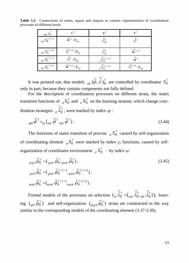
53
Table 3.3. Connections of states, inputs and outputs in canonic representation of coordination
processes of different levels
It was pointed out, that models are controlled by coordinator
only in part, because they contain components not fully defined.
For the description of coordination processes on different strata, the states
transition functions of and on the learning stratum, which change coor-
dination strategies , were marked by index :
}ˆ,ˆ{ˆ o . (3.44)
The functions of states transition of process caused by self-organization
of coordinating element were marked by index χ; functions, caused by self-
organization of coordinator environment – by index ψ:
, (3.45)
,
.
Formal models of the processes on selection learn-
ing and self-organization strata are constructed in the way
similar to the corresponding models of the coordinating element (3.37-3.39).
0
C X Y
1/0
So xEW /~
0
~C G
~
1/0
So xEG /~ 1
0
~C
1~ W
1/0
S yEG /~ 1/
0
~ CW
~
1/0
S yEW /~ 1 1/
0
~ C yEG /~ 1
0)ˆ,ˆ(
0S
0So
0S
0
0S
0So
0S
}ˆ,ˆ{ˆ 000 o
}ˆ,ˆ{ˆ 1/0
1/00
ooo
}ˆ,ˆ{ˆ 1/0
1/00
}),ˆ,ˆ{ˆ( 000 o
)ˆ( 0 )ˆ( 0

54
3.2.3. Description of coordinator environment
The development of the model of coordinator environment is conducted in a
similar way as that of the coordinating element, bearing in mind the following facts.
Coordinator of each concrete systems being designed is the connecting unit
of lower , and higher , levels. For , the both coordina-
tors and coordinator are in direct contact with coordinator of level
(trough and respectively) and form its environment .
Coordinator connections with other coordinators of level
also go through its structural elements and , in other words, trough higher
and lower levels:
, (3.46)
.
Therefore, canonic representation of coordinator environment is
decomposed into two classes of models:
(3.47)
and their states spaces were marked as and respectively:
(3.48)
States space of coordinator environment is constructed just as the
states space of the coordinating element (3.31) in the following form (3.49):
(3.49)
The elements of the abstract systems given in
(3.48) form represent the following states. represents the states of system
structure and represents the state of aggregated dynamic real-
0S
0S S
0 0 11
0S 1
0S
0S
S1 0S
0S 1
0 , IiS i
}},,{,{ 1/0
1/00
},,,{ 111/0
WG },,{1/0
GW
0)ˆ,ˆ(
},)ˆ,ˆ(,)ˆ,ˆ({)ˆ,ˆ( 1/0
1/00
1/0
C1/
0C
}.,{ 1/0
1/00
CCC
0C
0S
},,,{/~
000000 CCCCECC c
},{ 1/0
1/00
CCC
1/0
C S 1/
0C

55
ization of the system being coordinated – designed and controlled. Their
connection is defined as follows by the law which arose from (3.27):
( ) {
& (3.50)
& { )]ˆ(&)ˆ(&)ˆ)(ˆ()[( 321 tttttttT
Law represents the connection of structural elements and of
coordinator , in other words . means that that level of in-
formation uncertainty in is higher than the one in ; becomes suffi-
ciently defined only when system of level becomes sufficiently de-
fined.
As a result, coordination signal and feedback
become determined for when the system of a higher level has been formed.
This definition is relative because of the synthesis and functioning laws of systems
of level can change the higher levels.
Canonical representation of coordinator environment is spec-
ified as follows:
: , (3.51)
Decomposition of states space into and resulted in
the corresponding decomposition of canonical representation . For
, the decomposition is presented in the following form:
:
,
S
s
)]"(&)"(&)")("()[( 321 tttttttT
)}( T
)}.( 1 T
0S
0
1S 1
11 G 11 Ww
0S
0ˆ S
0S
0)ˆ,ˆ( }'&',&:ˆ{ˆ 0'00'00 ttTttCYC tttt
}.&~~
:ˆ{ˆ00000
TtXYCt
0C
/0C
/
0C
0)ˆ,ˆ(
1
1/0)ˆ,ˆ(
}'&',&:ˆ{ˆ 1/0'
1/0
1/'0
1/0 ttTttCGC tttt

56
, (3.52)
:
}'&',&:ˆ{ˆ 1/0
1'
1/0
1/'0
1/0 ttTttCWC tttt
,
.
Functions and are decomposed in the same way as for co-
ordination strategies (3.38) and define the formation ways of feedback and
coordination signals under conditions of different information uncertainty
indexed by . The states transition function , similar to
and functions, contain two strata – learning ( ) and self-
organization (0 ).
The task of the self-organization stratum 0 for coordinator environment
is to change the level of system from to . The task of self-
organization stratum 0o of coordinating element is to install the struc-
tural connections of formal model for level , in
other words to change state from to .
The structural elements of aed formal model are its basic terms , ,
, , , , etc., which are at the same time connections in . For ex-
ample, system connects , and ; coordinator connects and
in ; dynamic realization connects , and ; process
connects systems and , for which plays the role of their
interconnections; and are the environment for , and processes
and are structural elements of , etc.
}&~~
:ˆ{ˆ 1/0
1/0
1/0
TtWGCt
1/0)ˆ,ˆ(
}&~~
:ˆ{ˆ 111/0
1/0
1/0
TtGWCt
1/0ˆ
1/0ˆ
W
1G
},,,{ L0
0o
0
0
0S
S
0So
))(( S TS
TS 0S
0S
S S 0S
S S
S 0S
0S
S ~ 0S S
S
SSo
SS
SoS
S
SoS
S

57
Each structural element of system must be defined on self-organization
stratum of coordinator by its formal model, i.e. by aed . In aed model
the following components must be indicated: aed structural elements (with their
dynamics) and their connections, i.e. structure of aed, its connections with
other elements of in general model , i.e. dynamic realization of
aed, and the restriction on aed coordinator which defines the ways of concreti-
zation of both and .
In other words, on self-organization stratum coordinator performs the sys-
temic analysis of each element of formal model in terms of this model and
synthesizes the abstract system . In this way controls the conformity of
the system model to the laws of synthesis and functioning of an traditional concrete
system of level , which is created by both coordinator and environment .
3.2.4. Performance of the design task of mechatronic systems
Design tasks of mechatronic systems and control process are distributed on coordi-
nator strata: selection, learning and self- organization (self-coordination). The
task is partially described in [49] as well.
On the selection stratum at moment of time, predicting the environment
systems states for moment , coordinator defines correspondent inputs and
outputs of the system being designed and creates models of the system
and its process using the obtained predictions. After that, coordinator selects such
states of subsystems and their interactions which correspond to the standard state
of system required for , i.e. performs the task of structure synthesis of
the object being designed.
The synthesis task is formalized by introducing interlevel relations on infor-
mation resources of abstract aed model Ψ = Ψω × Ψσ [3, 49-50], where Ψω is a
relations net on the multitude of dynamic systems , Ψσ is an analogous net
of relations × with the types of structures . Ψσ contains, in particular,
TS
0S TS
S TS
0S
0S
S
TS0S
0S S
0S
Tt
tt '),(
S 't So
),(

58
equivalence relations on structure types by the connection defects, construc-
tive dimension and way of subprocesses organizations (continuous, parallel con-
nections and feedbacks). Adaptation of structural model to the concrete appli-
cation area, i.e. mechatronic system design, is executed by the indication of con-
crete external model ∈ Ψω and class of structures which contains external
models of elements (subsystems ) of system
under consideration
being designed.
Structure classes – space of mechatronic system constructions – for the de-
fined elements basis correspond to a certain way of designed system functioning.
Technical constructions for each way of functioning are selected by changing pa-
rameters of the designed object subsystems and their interactions σ,ωγl. The
change of the parameters causes the change of external model of the mechatronic
object. It allows finding out if the required state of designed object is obtained
(analysis task). We return to the synthesis task if there is incoherence of the ob-
tained and standard states of the object being designed.
The choice of parameters of the designed object structure depends on the un-
certainty level of the coordinator information about the environment S . For
each level of information uncertainty the equivalence classes of the coordinator
states in the design process are introduced. Each class of states of the coordinator
has its own coordination strategy: coordination of interconnections, evaluation of
interconnections and the prediction of interconnections (most exact) described in
Section 3.2.1. Coordination strategies (3.38) are realized on the selection stratum.
On the learning stratum the coordinator fixes the level of information uncer-
tainty. It compares the data about the environment systems received by the feed-
back and the same data contained it its informational resources (data bases). In this
way the required area Ψ of informational resources is defined. In the frames of this
area the selection of required technical construction of mechatronic object will be
done. Corresponding state of the design process (coordination strategy) at the se-
lection stratum is also defined.
Information resources Ψ of the coordinator are changed in the design process
on its self-organization (self-coordination) stratum. The reason of the change could
be the absence of coherence with the real mechatronic systems model in infor-
mation resources Ψ. The criteria for including a new model into Ψ is the exactness
of the solutions obtained with the help of the model.
1 1S S
1S
So
0S

59
3.3. Metrical characteristics of hierarchical
mechatronic systems
Structural-dynamic connections of S ,
0S , ,
, 0 , s , elements of
formal model S of aed – the standard formal element of design and control sys-
tems – realize the main laws of hierarchical systems. Numerical characteristics
necessary for further investigation of the laws and quantitative measurement of
particular mechatronic systems being designed are introduced in this Chapter. All
numerical characteristics of hierarchical mechatronic systems are determined be-
low by the means of positional numeric system sL .
3.3.1. Levels of mechatronic systems
The most general numerical characteristic of hierarchical mechatronic systems is level
L , where: sLL ,
sL is numeric positional system (generally with an unfixed
base), specified on multitude }&&),(:{ LILILs , L is
the multitude of indices of levels, I is the finite set of indexes on level , the base
on each level is marked by symbol ,
NN , is the set of natural numbers.
L is determined as ,}{ ELL s
E are relations of equivalence on
ss LL :
]."'),)[(,)(,( "'"'"' ELs
(3.53)
Abstractive mapping is marked with symbol R :
,: LSR ,},,{: 0 LSR
(3.54)
which sets correspondence of mechatronic system S and the index of its level.
For dynamic and structural
representations, the reflections are
defined as follows:
,: LR
.: LR
(3.55)

60
To determine dynamic t and structural
t presentations as the restrictions
of 0 and
0 at time
tT :
Tt
t
~
,
Tt
t
~
, the following definition
was made.
Definition 3.5. (i) Space of dynamic realizations of hierarchical mecha-
tronic system on levels L is called a factor set of system
E~
, where
E are the relations of equivalence on
~~
:
)].()(),)[(~
,)(,( 21212121
RRE (3.56)
(ii) The space of structures of hierarchical mechatronic system on levels
L is called factor set
E~
, where:
)].()(),)[(~
,)(,( 21212121
RRE (3.57)
Systems iS and
S are considered as equivalent by their level independently
of the equality of their bases i and
. In other words, the might be systems
with different bases on one level. Equivalence
E is determined on ss LL
for their classification:
)].(),)[(,)(,( "'"'"'"'
ELs
(3.58)
Spaces and
are constructed as factor sets
E~
and
E~
by analogy with and
as follows:
)]()(),)[(~
,)(,( 21212121
RR ,(3.59)
)]()(),)[(~
,)(,( 21212121
RR , ....
.:,:
LRLR
Validity of property for state space C follows from s and R :
( ) &))(( CcSR (3.60)

61
& &?)&)(( 0 tCcSR
& &?)&)(( 0 tCcSR
& ?).&)(( 0 tCcSR
Property connects the values of the level of mechatronic system S with
values },,,{ L of the levels of system organization and coordinator’s
0S information uncertainty. means that each mechatronic system
S
spreads at least over three levels up and down in L . The levels’ indices in interfac-
es with natural languages may be replaced by words (machine part, module, ma-
chine, etc). Levels on which the reference models introduced are adjustable (by the
change of parameters) to any system of this level are called strata.
Levels },,,{ in 0 are called:
– the levels of information uncertainty – for signals ,
1 , w ,
1w ;
– the levels of system organization – for coordinator’s environment 0S .
Levels },,,{ also encode output functions 0 as coordination strate-
gies on the selection stratum of coordinator.
3.3.2. Numeric positional system
Formal models of aed and coordinator, as a theoretical basis for the design method
proposed in the book, are constructed with the help of their most important particu-
lar cases – dynamic system ),( and numeric positional system sL .
sL allows
determinations of level to be easily introduced.
The dynamic systems are algoristic and sufficiently investigated. But for nu-
meric positional systems there is no formal model in spite of its big importance in
numeric information processing.
Numbers in a positional code are usually presented as polynomials, which are
not in coordination with most characteristic features of sL , i.e. with the realization
of interlevel transitions in aggregated presentation of numbers. So, addition of
numbers in a positional code usually leads to the degree of the result being higher
than that of the items. This is impossible for the group of polynomials of degree n
which are closed with respect to the addition operation. Furthermore, system sL

62
can’t be formalized by the means of any other one-level mathematical model ei-
ther. Being hierarchical by nature sL is formalized only in terms of hierarchical
systems theory.
It is sufficient to examine model sL for one standard block which is repeata-
ble on each of its level. This block is constructed on the following basic system T
~ :
~~,~~,~~,~~~
T , (3.61)
),,,(,~,),,,(,~
,~~ 0
,
),,(,~,),,(~,~,~~~ 00 ,
)(?,,?~
,?),(~,~,~~~ 00 ,
~,~,~~,~,~~~ 000 ,
),,,(),,,( ,
),,,(),,,( .
The meaning of symbols },,,{ in T
~ is coordinated with the mean-
ing which they have in canonic model 0 of coordinator, where λ is the index of
the most organized system, φ and χ are partly organized ones, ψ is an unorganized
system. Property (Fig. 3.3) sets connections between systems T~
, T
~ ,
T~
and T~
( , 1 , 2 , 3 ). The whole
system T
~ turns into the neutral element 10~
1~
T of the higher level.
Element
~0, which is the connection of positively and negatively oriented ele-
ments
~ and
~ is decomposed into elements of level 1 in T
~ .
Bilateral symmetry of elements ~i and
~i (where },,,{ Li )
corresponds to the direct and reverse states transitions of system S in self-
organization cycle.

63
Diagram (Fig.3.3) is in coordination with and . When struc-
ture is in state λ, i.e. the system has level , aggregated dynamic representa-
tion (for ?01
t ) is in state φ (level ). When the state index of is
equal to φ (level ) and ?01t , the index of
is χ, etc.
Fig. 3.3. Scheme of inter-level relations ,~ iT
},,,{ Li
It is shown that Figure 3.3 is analogous to aed S model in its canonical
presentation. The arrows illustrate the elements’ inter-level connections which go
through coordinator 0S . System dynamics on each level is specified by the se-
quence of transitions from ~ to
~,
~,
~ and vice versa, which is for-
malized by canonic model 0 of coordinator.
The change of states },,,{ of level of system
sL from the state of
absolute information uncertainty and the weakest organization to relative de-
terministic state is accompanied by alteration of
sL characteristics of its
higher and lower levels. The relations between the values of numeric characteris-
tics of sL for different levels are determined in the following (3.62) form.
Here 1 is a unit of level ; diverse levels have their own bases 1 ,
,
1 , 2 ,
3 are not necessarily equal. Unit of level is regarded as 10,1
1) (
) (
1) (
1) (
) (
1) (
1) (
1) (
) (
ℓτΨ:
1) (
( )

64
on level and unites =10 units of level -1. Each system
S is connected
through interactions with the other systems of level which create environ-
ment S of system
S . is called a prolongation of system
S in its envi-
ronment S and marked as
S~
:S
~=
.
( )
1
2 3
1 = 10,1 = 20,01 = 30,001 (3.62)
║ 110 ( )LS
)( )1( SL
System sL of level with its prolongation sL
~ in environment
sLS is
described and presented in Figure 3.4.
SL
SL~
1
0i
i k ~ 1 1
0,~ i
1~
~ i
i001~
i k0 1~
1
0,
0 ~ i
1~
0 ~ i
i ~0
1
1~ ki
1
0,~ i
1~
~ i
~T 1
)~
,( SS LL
~T 1
Fig. 3.4. System SL and its prolongation
SL~
in environment sLS , where:
1~ ki – element of
k number of basic system 1~ T , i – index },,,{ Li ; )
~,(
SS LL – interaction of
systems SL and
SL~
X Y

65
Theoretical construction of aed-processor which is oriented at the processing
of numeric and geometric information of mechatronic system being designed is
defined as a structure of three connected levels of system sL . Construction of
aed-processor is presented in Figure 3.6.
For system sL in Figure 3.4,
elements of the lower level are determined
on multitude 1~
T , the base of system
sL~
is equal to ~ and sometimes may
not coincide with (
~ characterizes the quantity of sL connections in
sLS ). Elements of sL~
are transferred by system sL to the other systems of
its level. In particular, the whole system sL
~ can be transferred to only one system
1, IiLsi . The relation of
sL and sL
~ systems goes through element
)1( sL
=)1(
0
~ sL . Number
defines the address of interactions ~ (sL ,
sL~
) in sL ,
which is coordination signal sL for system
sL .
Fig. 3.5. Connection of discrete elements of system sL continuous in time, where:
sLS |0
– coordinator
of sL ;
sLC |0
– states of coordinator environment [140]
sLC |0
sLC |~
0
sLS |0

66
System {sL ,
sL~
} in its initial state contains non-oriented elements only. The
uniting of elements with different orientation which come to the input of sL gives
a non-oriented element again. When the quantity of elements with the same orien-
tation is equal to , signal
sLw 1 (unit 1 of level , i.e. 0.1 of level 1 )
goes to higher level 1 informing that system sL has passed into its organiza-
tion state λ, see (3.61).
The further process in sL is illustrated in Figure 3.5 and described as follows.
Being in its organization state λ (3.61), each system s
iL gives its prolongation
siL
~ to system
siL 1 and after that
siL 1 begins to receive the inputs of level (in
the moment of prolongation transfer it may occur that s
iL~
contains a certain num-
ber of elements with the same orientation). In this way, discrete systems s
iL and
),( 1 IiLs become continuously connected.
yl
yl-1
i
l-
i
+
i
l
0
i
l
xl+1
yl+1
xl-1
i
xl
Fig. 3.6. Aed-processor construction, i.e. three connected levels of SL , where:
yx , – inputs
and outputs of level ; ~i – element of basic system
T~
[140]

67
It is necessary to point out that information for higher levels is aggregated and
the sizes of units of different levels with equal bases are equal.
Each level in sL has its own inputs and outputs sL . Interconnections
sL of system sL of level go through structural connections
sL
which connects elements )1( sL of system
sL . The connections in sL have all
the features of the process of addition in column. When one unit of the higher level
goes to the left, part of the sum stays in its position in sL
~ for the following addi-
tion operation.
The change of states ),,,( of system
sL is executed by its coordinator
sLS0 through states transition function sL0
sL0 (Fig. 3.5). For the con-
nection of sL with the fields of real (ℝ
), complex (ℂ
) and with hyper-complex
(ℤ) numbers the multiplying operations on corresponding contractions of
T~
are considered below.
The multiplication in the field of real numbers is determined by states transition
function )()ˆ( R0R SL (Tab. 3.4) on contraction T
~R of system
T~
:
T~
R}
~,~,
~{
&
~~ (3.63)
where ~ plays the role of zero, and
~
are the units.
Table 3.4. Multiplication in field of real numbers
)(R
X
C φ
φ
φ φ φ φ
φ
Table 3.5 of function of states transition )ˆ()( 0CC
SL defines the mul-
tiplication of complex numbers on the contraction T
~C
}~
,~,~,~,~
{
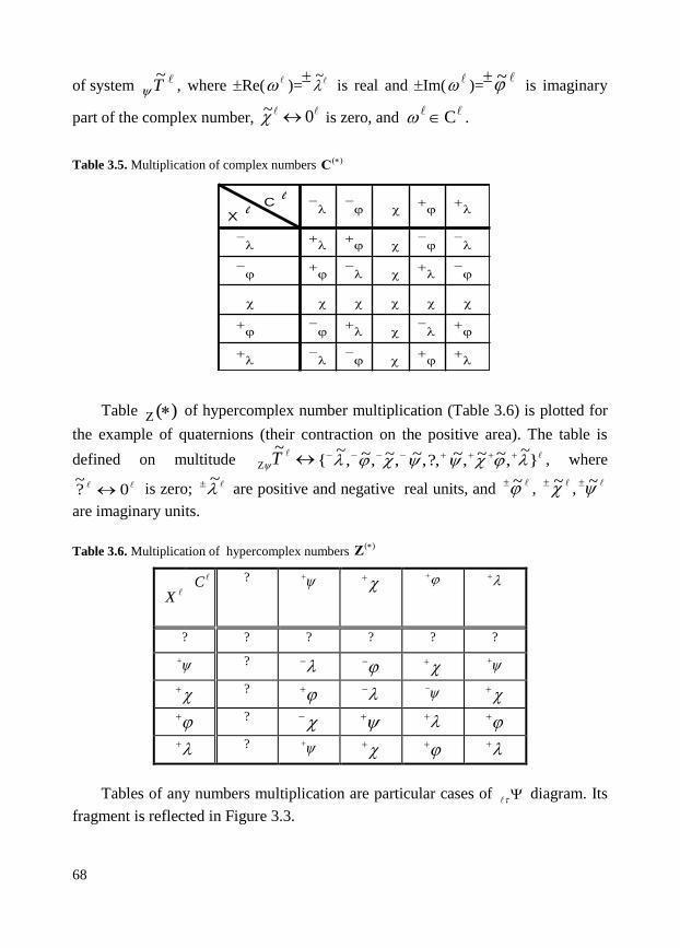
68
of system T
~ , where Re(
)=
~ is real and Im(
)= ~ is imaginary
part of the complex number, 0~ is zero, and
C .
Table 3.5. Multiplication of complex numbers )(C
Xl
Cl
Table )(Z of hypercomplex number multiplication (Table 3.6) is plotted for
the example of quaternions (their contraction on the positive area). The table is
defined on multitude T~
Z}
~,~~,~?,,~,~,~,
~{ , where
0?~
is zero; ~ are positive and negative real units, and
~,
~,
~
are imaginary units.
Table 3.6. Multiplication of hypercomplex numbers Z( )
X
C
?
? ? ? ? ? ?
?
?
?
?
Tables of any numbers multiplication are particular cases of diagram. Its
fragment is reflected in Figure 3.3.

69
The multiplication law of any elements of system T
~Z (Table 3.6) is im-
plemented as follows:
– index },,,{ ci of state element ci
~ defines ci
~ in the initial state
of system
0
~T , where (conditional) the origin of coordinates is
~
;
– index xi of input element xi
~ (coordinating signal) identifies level
},,,{ xi from which system tT will be considered, i.e. identifies a new
origin of coordinates;
– ci
~ elements in new coordinates are transformed into other elements T,
i.e. their indices change, which is illustrated by diagram and multiplication
tables )(R )(C , )(Z ; the process of indices transformation runs in such a
way that the results of any table line cannot be the same for any other line.
For instance, when system R T }~,~,~{}~,~,~{ 0
is multiplied by
~ , its state does not change and both elements
~ (unit) and
~ (zero) stay in their places. When R T
is multiplied by
~ , index λ of the
origin of coordinates goes into φ, i.e. φ is replaced by λ, and vice versa λ is
changed by φ (element
~ on level comes into
~ and
~ comes into
~ ).
It should be pointed out that for the multitude of real numbers in sL code,
)(R table is insufficient and a diagram similar to )(Z is required. The diagram
is also a particular case of . For instance, the real and complex numbers multi-
plication in sL positional code (which may be also reduced to addition in sL ) is
obtained from by the following way. The addition of )10( real units
1~ of level 1 is equivalent to multiplication *~ 1
, i.e. 0.1*10 or
multiplication 1~
1~* of units of levels 1 and 1 .
Both indices 1 and 1 of units of level λ are equal to φ and these units
for can be recognized as imaginary ones, i.e.
~~ 1 ,
~~ 1
and imaginary numbers
~*~ are multiplied.
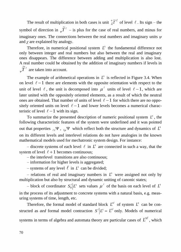
70
The result of multiplication in both cases is unit
~ of level . Its sign – the
symbol of direction in T
~ – is plus for the case of real numbers, and minus for
imaginary ones. The connections between the real numbers and imaginary units ψ
and χ are explained by analogy.
Therefore, in numerical positional system sL the fundamental difference not
only between integer and real numbers but also between the real and imaginary
ones disappears. The difference between adding and multiplication is also lost.
A real number could be obtained by the addition of imaginary numbers if levels in T
~ are taken into account.
The example of arithmetical operations in sL is reflected in Figure 3.4. When
on level 1 there are elements with the opposite orientation with respect to the
unit of level , the unit is decomposed into units of level 1 , which are
later united with the oppositely oriented elements, as a result of which the neutral
ones are obtained. That number of units of level 1 for which there are no oppo-
sitely oriented units on level 1 and lower levels becomes a numerical charac-
teristic of level 1 with its sign.
To summarize the presented description of numeric positional system sL , the
following characteristic features of the system were underlined and it was pointed
out that properties , which reflect both the structure and dynamics of sL
on its different levels and interlevel relations do not have analogies in the known
mathematical models used for mechatronic system design. For instance:
– discrete systems of each level in sL are connected in such a way, that the
system of level 1 becomes continuous;
– the interlevel transitions are also continuous;
– information for higher levels is aggregated;
– systems of any level in sL can be divided;
– relations of real and imaginary numbers in sL were assigned not only by
multiplication but also by structural and dynamic uniting of canonic states;
– block of coordinator sLS 0 sets values
of the basis on each level of sL
in the process of its adjustment to concrete systems with a natural basis, e.g. meas-
uring systems of time, length, etc.
Therefore, the formal model of standard block sL of system
sL can be con-
structed as aed formal model contraction sLS sL only. Models of numerical
systems in terms of algebra and automata theory are particular cases of sL , which

71
is caused by the ways of its formalization [3,8-10]. The system for geometrical and
physical objects measuring in H. Lebesque theory [48] is also a particular case of
sL .
The possibility of physical realization of sL arises from its coordination with
natural processes of calculation performed in positional codes. That possibility is
partly illustrated by Figures 3.4-3.6 in which sL is reflected by analogues of mod-
ern calculating machines.
3.3.3. Measuring units of mechatronic objects
To introduce the measuring units of hierarchical mechatronic objects, the following
definitions are formulated. Previously, it was pointed out, that states of mechatron-
ic system S are indicated by symbols of
sL , i.e. they could be of different levels,
orientation or neutral on each level. Their interlevel dynamics is defined by scheme
(Fig. 3.3).
Definition 3.6 (i). Any neutral state Cc iti
i , where
ii Tt is the minimal
element of
iT , is called initial state i (the unit from
i for measuring S )
for any period of time },,,{ TTTTTTi of system
S . Multitude
CH iii }{~
is called the object of initial states for
iT .
(ii) For any period of time TTi any neutral state
Cc iti i is called the
standard state, or measuring unit , where
it
~ is the maximal element of
iT .
Multitude CH iii }{
~ is called the object of standard states for
iT , .Li
It follows from s (3.27) that the standard state of each period TTi is
the initial state for period TTi 1 :
11
~
iii H .
Definition 3.7. Set }~),,~({ ss S is called metrical characteristic
s
~,
S ),~( Ss of mechatronic system S in relation to standard
s~ , where
),~( Ss is the measure of S in units
s
~.
Metrical characteristic concerning the initial state is identified by analogy.

72
The representation of metrical characteristics:
),~( , ),~( , (3.64)
),~( ccc , ),~( xxx , ),~( yyy ,
),~( cxc ,
for or
, states of object So , processes
So , S and for environment
S , respectively, allows a range of state spaces to be constructed in addition.
Metrical characteristics are dimensional qualities and are con-
structed from two elements, one of which – measure – is the number in sL code
and the other one is any unit of measurement.
It should be pointed out, that the metrical characteristics of object So , pro-
cess S and environment
S are connected with one another by relations
determined by aggregated dynamic realization . Metrical characteristics
and are connected by interlevel relations realized by coordinator
0S . The
connections for each particular mechatronic system are defined by its formal model S .
Preliminary conclusions
In Chapter 3, the element of theoretical basis of HS design method – the aed for-
mal model of coordinator – was constructed with the help of the dynamic system.
Coordinator’s state spaces concerning the level of its information uncertainty were
introduced. Canonical presentation of the coordinating element, the process of
coordination and the environment of coordinator were built in the state spaces ob-
tained.
The design task of mechatronic systems is performed by coordinator on its
strata by one of its coordination strategies. Strategies of selection strata were de-
scribed by the output functions of canonical model. Change of states of coordinator
was described by states transition functions, which correspond to the functions of
leaning strata (change of coordinator’s strategies) and functions of self-
organization strata (change of the state of the formal model). Coordinator actions

73
while performing the main design tasks of mechatronic objects – synthesis and
analysis – were described.
So, the model developed meets the requirements of the design systems formu-
lated in Introduction and Section 3.1 of this Chapter.
With the help of numeric positional system, connections of levels and metrical
characteristics of the hierarchical mechatronic objects being designed were intro-
duced. The known numeric systems were subsequently described with the help of
hierarchical systems. All this allows quantitative calculation on the space of levels
of the designed mechatronic objects to be executed. Such a description causes real-
ization of coordinator in the form of the theoretical construction of aed-processor,
i.e. cybernetic system oriented to numeric and geometric information processing.
Theoretical basis of the conceptual HS design method, i.e. aed formal model
presented in this Chapter 3, was improved in comparison with its previous version
described in [140], and has got the following additional characteristic features:
general scheme of aed (Fig. 3.1) has improved so that system S block became
included in its environment S ; all elements of aed model were presented in the
form of systems with correspondent indexes from the set },,,{ ooLk ,
which indicate object ),(o environment )( , and their processes )( o and )( ;
symbol presentation of systems connections was changed from U to
what
made it agreed with presentation of coordination signals 0 generated by coordi-
nator while performing systems structures synthesis in design process by arranging
subsystems structural connection; fundamental aed law of systems levels grows
was modified by the law of systems outlook increasing in the levels space, i.e. in-
creasing of number of system levels being coordinated ‘up’ and ‘down’ in
regard with current level of system under consideration; symbols set of levels of
system organization L and correspondent basic system T
~ were changed to
},,,{ L and improved in such a way, that they become coordinated
with coordinator canonic model )ˆ,ˆ( and its reactions and functions per-
formed on selection and learning strata respectively. Furthermore, modified aed
model presented in this Chapter was further improved. New aed formal model for
systems design and control was presented and described by Novikava and Miatluk
in [8], and used after that by Miatluk and Kim in [80].
74
4. DESCRIPTION OF THE DESIGN METHOD
The formal models of hierarchical mechatronic objects and coordinator given
above in Chapter 3 are used in this Chapter for the description of both mechtronic
system (MS) being designed and the design process itself. Each mechatronic sys-
tem can be presented at the conceptual design phase according to (3.1) in the fol-
lowing aed form (4.1) of HS:
},,{ 0 SS mm , (4.1)
where: m is the dynamic representation of mechatronic system
Sm as a unit in
its environment Sm ,
m is the structure of the system Sm ,
0Sm is coordina-
tor, which connects m with
m , m is the index which indicates the mechatronic
nature of the object being designed.
The states of a mechatronic system in its and
forms are detected by its
metrical characteristics. Aggregated dynamic (functional) representation of mecha-
tronic system (MS) is described in accordance with (3.11):
m =m{ ,o
, , , , }, (4.2)
where: ,o – dynamic description of mechatronic object (MO) itself,
,
– description of the mechatronic process (see Subsection 4.4.2),
, – dynamics of the MO environment (external representation).
An examples of the description of MO dynamics by ,o is presented be-
low in Subsection 4.4.2.
Structure m of mechatronic object is presented according to (3.14) in the
following form (4.3):
}},{,{ 10
Smm , (4.3)
75
where 1 is a set of mechatronic subsystems of lower level -1 and their struc-
tural connections .
Coordinator 0Sm is the system which sets the characteristics of mechatronic
object elements and coordinates their connections by the sequence of operations
and the decision-making actions, such as a choice of the decision and the construct-
ing of semantic net on the MO elements set. These actions include the operations
of MO metric characteristics changing, operations with MO geometric elements
structures and their connection.
So, to construct an mechatronic object it is necessary to define its structure, its
function – aggregated dynamic representation as the unit in its environment, its
environment construction and technology, MO coordinator (design and control
unit), and their metrical characteristics.
The main design tasks – analysis and synthesis – of mechatronic objects are
performed by coordinator 0Sm on its strata (see Chapter 3) under conditions of
different information uncertainty. 0Sm creates the desired construction of mecha-
tronic object in accordance with its required dynamic functional representation in
the environment (synthesis task). In its turn, it partly changes the structure parame-
ters of the resultant mechatronic object and analyses its behavior in the environ-
ment (analysis task). All the tasks are performed at both Conceptual Design (CD)
and Detailed Design (DD) phases of mechatronic object life cycle using HS design
method, i.e. coordination technology of HS.
So, the main steps of the HS design method realization are the following.
1) Conceptual model creation – description of the mechatronic object being
designed in aed form of HS; aed is a standard block of hierarchical systems – for-
mal analogue of two-level system with dynamic units.
2) Representation of basic geometric elements (point, line, surface, 3D ob-
ject) of the mechatronic object being designed in the hierarchical form – condition-
al point, line, surface, 3D object.
3) Definition of metric and constructive characteristics – constructive dimen-
sion and connections defect – of the mechatronic object being designed in the
codes of numeric positional system.
4) Realization of the design process of mechatronic objects – synthesis and
analysis tasks performing – as the coordination process of aed.
At the first step of the method realization – conceptual model creation – the
connected formal models of the mechatronic object structure, its dynamic func-
tional representation as a unit in its environment, the object environment and the
environment processes are developed (see Chapter 3). Formal descriptions of ob-
ject-environment interactions, mechatronic object coordinator and its coordination

76
(design and control) processes, processes executed by subsystems and general pro-
cess are presented as well.
At the second step, the representation task of basic geometric elements of the
mechatronic object being designed in the hierarchical form is performed. The rep-
resentations of MO geometric elements in HS forms of conditional point, line,
surface and 3D object are described in details below in Subsection 4.3.
At the third step, definition of metric and constructive characteristics of the
mechatronic object being designed is performed with the help of numeric position-
al system Ls. Main numeric characteristics of MO – constructive dimension and
connections defect – are introduced in Ls basis. Formal definitions of these charac-
teristics are presented below in Section 4.2.
At the fourth step – synthesis and analysis tasks performing – the conceptual
descriptions of the tasks are presented first. The task of MO structure synthesis is
given in the following form of the coordinator mapping:
},{: 1
0S
(4.4)
where MO structure which is synthesized from set of sub-subsystems 1S
presented in aggregated dynamic forms 1 by establishing of the structural con-
nections of these elements 1S .
The steps of the synthesis process 1S are formally described by reaction of
dynamic system :),(
}&:{ TiYXC iiii , (4.5)
where i is a time moment of the synthesis process, initial element (or composition
of elements previously connected in the synthesis process) is recognized as state
Ci, at the step i, element to be added to initial one is recognized as input Xi, and the
composition of the both connected initial and input elements is recognized as out-
put Yi. The output Yi becomes the state Ci+1 at the next step of the synthesis pro-
cess.
The analysis task of MO is performed by coordinator and presented at CD
phase in the following form of the coordinator mapping:
},{: 10S
(4.6)
In this task, coordinator partially changes the structural connections of
MO by sending its coordination signals to MO structure and observe the variations

77
of MO behavior – change of MO functioning in its environment caused by MO
structural variations.
While performing analysis tasks, e.g. kinematics and dynamics tasks, concep-
tual models of MO are presented at CD phase in ),( form. At the DD
phase the conceptual models are concretized and presented in forms of DE, State
Space Equations or algebraic form. The exemplary scheme of MO conceptual mod-
el concretization at the design phase of the object life cycle (Fig. 1.2, Chapter I)
is presented in Fig. 4.1.
Fig. 4.1. Steps of conceptual model , concretization at the design phases of MO life cycle; con-
ceptual model is transformed to ordinary DE at CD phase and concretized at DD phase by the exem-
plary dynamics equation of object being in rotational motion, where ω(t) is the angular velocity and is
T(t) is a torque
Synthesis and analysis tasks of geometric constructions of mechatronic objects
being designed are partially described in Chapters 6-8 as well. The steps of the
above HS design method are described below in Chapters 5-9 for the cases of the
exemplary mechatronic objects design tasks. The method is also partially regarded
in [49, 51-54].
4.1. General geometric characteristics of mechatronic objects
For the description of geometric elements of mechatronic object construction at the
second step of the HS design method realization the geometric information is pre-
sented according to (4.1) as a set of variables of three classes:
,,,, 321 , (4.7)
I
Conceptual
model
),(
DETAILED DESIGN phase 3 III
CONCEPTUAL DESIGN phase 2
Concrete DE
)()()(
)( tTtBdt
tdjtT Lm
mm
II
Ordinary DE
uayadt
dya 210

78
where: 1: Iii is the description of the state of geometric object
(with the help of metrical characteristics i which are the coordinates, length,
squares, volumes, angles) presented in aggregated dynamic form ,
2: Iii – is the description of geometric object interconnections
with other objects (boundary of the object defined by the coordinator),
3: Iii – is the description of object structure .
Then, any geometric representation of mechatronic object is presented in form
of relations S on the Cartesian product of variables ,, . Each
class of variables has its own structure, i.e. there are the sets:
},,{1 , (4.8)
where: is the structure of class , is structure of class, and is
structure of class .
Besides, there are gluing relations 2 between ,, . The multitude of all
the relations on is marked as : 21, .
One of the relations from 2 is . That means that the boundary of
each geometric object Sg is included in its structure . The boundary is the area
of geometric construction Sgm of mechatronic object Sm interconnections with
its environment S (i.e. defines the location of Sgm in S ). Each
corresponds to the coordination signal from coordinator 0Sgm to the object Sgm .
is defined through the interactions of the geometric mechatronic object Sgm with the higher and lower levels, i.e. measured with the help of its structural
units to be evaluated in its environment, and, inversely, being a unit of the envi-
ronment, it is measured with the help of the other environment units. So, the higher
and the lower level units for the object are its measuring units.
To construct geometric construction of mechatronic object Sgm it is
necessary to define all its variables , , . In design task any subset of parameters
from S must be initially defined. Other parameters are defined in the
synthesis process (Tab. 4.1).

79
The unknown variable (which is not presented in Z ) is marked in Table 4.1
by symbol ?. Definition of ? symbol is a task of self-organization strata of the co-
ordinator.
Taking into account the type of the design task and the knowledge level of the
coordinator, 0Sgm chooses the strategy of knowledge settlement, i.e. the algorithm
of the synthesis process.
Therefore, the structure of the design process is defined by:
– the dividing of set Z into known and unknown parameters (inputs and
outputs), i.e. the type of constructing task,
– by the geometric representation Sgm of the mechatronic object being de-
signed (concrete meanings of variables),
– by the uncertainty level of semantic net relations (former design expe-
rience).
Coordinator 0Sgm in this case plays the role of a system which defines the
characteristics of the elements set and coordinates their interactions with the help
of a sequence of actions and procedures of decision making.
These action classes include the procedures of the changing of metrical character-
istics as well as actions with boundaries and structures of geometric elements of MO.
Table 4.1. Subsets of parameters ,,Z in design tasks, processes and semantic relations
Design
process
Known
parameters
(input)
Unknown
parameters
(output)
Semantic net
relations
P,S , , S |S
P,S , , S ,|S
P,S , , S ,|S
P,S , , S ,|S
P,S , , S ,|S
P,S , , S ,|S
P,S , , S ,|S
P?, S ? , , , S , S

80
4.2. Numerical characteristics of mechatronic objects
To realize the third step of proposed method, all numerical characteristics of geo-
metric elements of MO (mechatronic object) S are described in the work and
connected with the help of numeric positional system SL presented in Section 3.3.
So, metrical characteristic M (measure of length, squares, volumes,
angles) is obtained in units },,,{ H , presented in Subsec-
tion 3.3.3, with the coefficients from SL :
~,~,~~ 0 , 11101
0~~,~,~~
, (4.9)
where: L , ~
– negative, ~0
– neutral, ~
– positive parts of ~ ; unit
~0 is at the same time a unit of lower level -1, etc. Numerical characteristics of
system S organisation – connection defect
~ and constructive dimension
~
were defined in the following way.
Let the object and the reflection
U R: be as follows:
}0{N&&&),(:),( + NNnLNLnn
,
ˆ,),()R( n
(4.10)
nnii )(R&}ˆ)R(:{)((
ˆˆˆˆˆ
,
Li
ˆ
R: , Nn R: , n – cardinality of ,
i – intercon-
nections of 1
iS in ; +N – natural numbers multitude,
SLL .
Then is called a connection defect of of order and cardinality n, and
})3,2,1,0{,()( IIL . (4.11)
The locations of the defects in MO structure are defined by parameter , :

81
:,..., 0, ii
(4.12)
ˆR(&&,:,,)0( ,iiIIiii .
For each system S of level L the connection defect in environment
S is called the contraction of connection defect , of system tS of higher
level +τ , sL on .
In the code of numeric positional system SL the connection defect is defined
as follows:
}.,{~
,...~
03 nn
(4.13)
The formal definition of constructive dimension and the ways of its calculation
are obtained from the definition of connection defect
~.
Constructive dimension of system S is called its numeric character-
istic, which is presented in SL code:
)()(},,{~
,...~
303 ii nnnn , (4.14)
where: ( )n Ni , i=0,1,2,3; and
are constructive dimensions of and
, respectively. The instance of constructive dimension ~
connection with
Euclidean dimension is presented by Table 4.2.
Table 4.2. Connection of constructive dimension
~ with Euclidean dimension
Constructive dimension
~
Geometrical object
S
0 0 0 1 Point
0 0 1 0 Line
0 1 0 0 Surface
1 0 0 0 3D object
Therefore, the described representation of geometric information allows all
operations with graphic images in aed-processor (subsection 3.3.2) to be executed
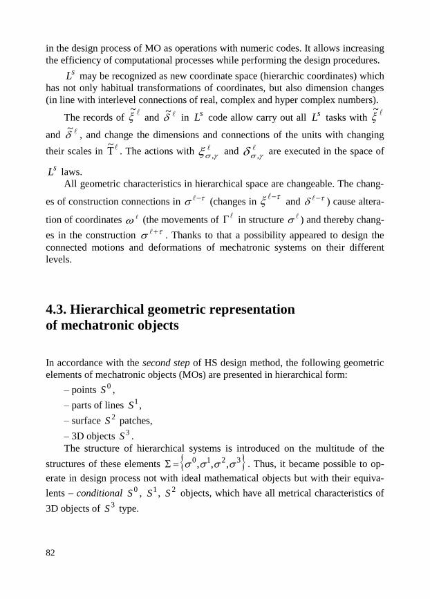
82
in the design process of MO as operations with numeric codes. It allows increasing
the efficiency of computational processes while performing the design procedures. sL may be recognized as new coordinate space (hierarchic coordinates) which
has not only habitual transformations of coordinates, but also dimension changes
(in line with interlevel connections of real, complex and hyper complex numbers).
The records of
~ and
~ in
sL code allow carry out all sL tasks with
~
and ~
, and change the dimensions and connections of the units with changing
their scales in
~. The actions with
, and
, are executed in the space of
sL laws.
All geometric characteristics in hierarchical space are changeable. The chang-
es of construction connections in (changes in
and ) cause altera-
tion of coordinates (the movements of in structure ) and thereby chang-
es in the construction . Thanks to that a possibility appeared to design the
connected motions and deformations of mechatronic systems on their different
levels.
4.3. Hierarchical geometric representation
of mechatronic objects
In accordance with the second step of HS design method, the following geometric
elements of mechatronic objects (MOs) are presented in hierarchical form:
– points 0S ,
– parts of lines 1S ,
– surface 2S patches,
– 3D objects 3S .
The structure of hierarchical systems is introduced on the multitude of the
structures of these elements 3210 ,,, . Thus, it became possible to op-
erate in design process not with ideal mathematical objects but with their equiva-
lents – conditional 0S , 1S , 2S objects, which have all metrical characteristics of
3D objects of 3S type.

83
4.3.1. Conditional point
The conditional point is described as follows. Conditional point S , where level =0, is a minimal element of geometric representation. In comparison with the usual
point it has all the characteristics of hierarchical systems:
0S ={ , , }0. (4.15)
Conditional point 0S can be graphically presented by a cube, a sphere, a pyr-
amid, etc.
Metrical characteristics of 0 (in case of cube) are: 00 – tops coordinates,
01 – length of edges, 0
2 – square of sides, 03 – cube volume.
The conditional point has the following qualities.
It may be constructed from lower level units (also points):
},,...,,{ 1
21
InSSSS n , (4.16)
but graphically its structure can’t be observed. Points 1
iS of lower level -1 have
the same type of structure but their metrical characteristics are smaller.
Each conditional point 1
iS can be in its turn decomposed into 2S . The
sequence of such decomposition operations leads to the ideal point with metrical
characteristics 01 =
02 =
03 =0.
In comparison with the ideal point, the conditional one has more operations of
coordinator: scaling (which does not take conditional points beyond their class)
and level lowering. In addition, the points can be united into a higher level system.
Thanks to that, it is easy to introduce the definitions of conditional line and surface,
which have all the characteristic features of ideal ones, and in addition, have their
own qualities.
As in the case of numbers, the point representation contains its positive (+),
negative (-), i.e. prolongation, and neutral (0) parts. In the coordinates it was pre-
sented as shown in Figure 4.2. In the case of conditional point interconnections in
the structure of higher level objects, the coordinates (directions of interconnections
in Fig. 4.2b) are defined by the structural addresses of the other elements of the
objects.

84
a) b)
Fig. 4.2. a) conditional point 0S with its positive (+), negative (-) and neutral 0, parts and metrical
characteristic 01 – length of the edge; b) directions of point interactions in the structure of a higher level
4.3.2. Conditional line
The part of continuous conditional line 1S is defined in hierarchical form as a two-
level system (aed) which contains the finite number of conditional points
0001 },...,{ SSS n . The points are ordered in a linear sequence in the structure of
line 1S , i.e. each point
0iS , i=1, ..., n has one preceding and one following points.
The main elements of aed definition for conditional lines 1S =1},,{ are:
– structure 1 as the finite set of conditional points;
– connections 1 ={ , }1 which contain structural connections
1 – the
sides and angles between conditional points, and external interactions 1 – any
point (or some points) from line structure, and/or boundary points 100
1 },{ SSS n
included into 1 ;
– aggregated representation 1 – the description of line as a unit with its met-
rical characteristics (for example, 10 are the coordinates of the points of the left
and right ends of the line, 11 is the length, etc.).
Coordinator 10S of line 1S can execute all operations with conditional points
which allow the points interactions to be coordinated in order to meet the require-
– –
–
+
+
+ + 01 –
0,S
0,
0S

85
ments to system 1S , i.e. the line equation. So, coordinator 10S can define all ele-
ments in accordance with the requirements to the system. When the boundary
points },{ 001 nSS coordinates
10 , line length
11 and the distance between the
centres of two neighbouring points 01 are given, then the number n of elements
0iS is precisely defined by the coordinator
10S .
The subset of the line structural points is called the basis of the line points.
The following quality is formulated as follows: in comparison with the ideal
line, the coordinator of conditional one realises operations of decomposition and
level rise.
The part of conditional line 1S in its 1 form is described by the same equa-
tion as the ideal one. So, the coordinator can execute the same operations with the
conditional line as with the ideal one:
– parallel transfer;
– rotation;
– continuous deformation (the elements 0iS and their number n are constant,
but elements interconnections l and locations are changed);
– the division into lines of smaller length (in comparison with the similar op-
eration with the ideal line, this operation, after the execution of finite n number of
steps, leads out of 1S class to class of points 0S );
– the continuous connecting of line 1iS with systems of the same class of lines
(this action leaves a line in class lS in case of saving linear order in the whole
system structure).
The set of relations on contracted on 1S , (1S ) is a set of
two-level systems (aed) relations. Thanks to that, the standard way of constructing
any system 1iS from class 1S was defined and it made possible to introduce new
variables in ,, .
The part of conditional line 1S , which is constructed from conditional points 0S (cubes) is shown in Figure 4.3. The figure is a screen-shot of the computer
where geometric construction of the conditional line was synthesised form condi-
tional points, i.e. cubes.

86
Fig. 4.3. Computer screenshot with conditional line 1S presented in its: a) aggregated dynamic form
,
and b) structural form , where: 0
1S – the first structural element; 0iS – any i structural element;
0nS – the last structural element, i.e. conditional point
One of the important manifestations of conditional line is its part. The part of
conditional line, as in the case of the ideal one, contains all point 0iS . The coordi-
nates of the points are defined by the following equation:
001
0 )1( ni SSS , 0, 1, (4.17)
where 01S and
0nS are the boundary points of 1S . Since the number of points
0iS
of line part 1S is finite, parameter has a discrete set of values (0, 1/n, 2/n, ..., 1).
Coefficients and (1-) are called a bury-centric coordinates or weight coef-
ficients of the points in },{ 001 nSS basis.
4.3.3. Conditional surface
Conditional surface 2S , or patch, is a two-level system which is composed of the
finite number of conditional lines which have a strictly linear order, i.e. each line
has only one preceding and one following relative line.
Conditional patch is also presented in form (4.1) as object 2S . Its characteris-
tics in general basis ,, , are defined as follows:
2 – is a two-level system’s (aed) structure defined above (which is
composed from the finite number of parts of connected conditional lines) and crite-
ria of lines selection;
01S
0nS
0iS

87
2 – a closed segment of conditional line and elements, i.e. conditional
points, which create the segment;
2
i with their metrical characteristics 2
i , i=1, ..., n connected by the
interlevel relations with the metrical characteristics 1i of the set of conditional
lines 1S which create surface 2S .
Coordinator 20S of system 2S can execute all possible actions with condition-
al patches. These actions allow lines 1S to be coordinated in the way meeting the
requirements to the whole system 2S .
The following qualities of the part of conditional surface 2S are defined as
follows.
1. Since each conditional line from 1S has a strictly linear order T, it is neces-
sary to have two parameters for the ordering of conditional points 0S of patch 2S ,
i.e. and t, t for points 0S of lines 1S ordering and for the ordering of
conditional lines of the patch 2S .
2. Any subset of conditional lines from 1S containing initial 1
1S and final 1
nS
lines is called a linear framework of the patch 2S . Interconnection points of any
two linear frameworks are called the framework of the points. Any framework is
simply defined by the boundaries and choice criteria of conditional points and
lines.
3. The contraction 2S of the relations set defined on for 2S
class is the set of two-level system relations. Thanks to that the standard way of
any system constructing from 2S class is defined.
4. Boundary 2 of conditional patch 2S contains not only conditional lines
but also elements 1S of conditional points which do not take part in these points
interconections.
5. The interconnections of two patches, or a patch and line, or a patch and
point and defined similar to the case of line in accordance with the general laws of
hierachical systems.
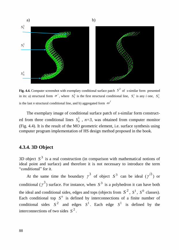
88
a) b)
Fig. 4.4. Computer screenshot with exemplary conditional surface patch of s-similar form presented
in its: a) structural form , where is the first structural conditional line, is any i one,
is the last n structural conditional line, and b) aggregated form
The exemplary image of conditional surface patch of s-similar form construct-
ed from three conditional lines 1nS , n=3, was obtained from computer monitor
(Fig. 4.4). It is the result of the MO geometric element, i.e. surface synthesis using
computer program implementation of HS design method proposed in the book.
4.3.4. 3D Object
3D object 3S is a real construction (in comparison with mathematical notions of
ideal point and surface) and therefore it is not necessary to introduce the term
“conditional” for it.
At the same time the boundary 3 of object 3S can be ideal (
3i ) or
conditional (3 ) surface. For instance, when 3S is a polyhedron it can have both
the ideal and conditional sides, edges and tops (objects from 2S , 1S , 0S classes).
Each conditional top 0S is defined by interconnections of a finite number of
conditional sides 2S and edges 1S . Each edge 1S is defined by the
interconnections of two sides 2S .
2S 1
1S1
iS 1
3S
1iS
11S
1nS

89
3D object 3S is defined on the basis of geometric variables ,, and
their relations in the following way:
3 is a two-level system (aed) composed of the finite number of con-
nected surface patches 2S and containing the criteria of patches selection;
3 is a closed conditional surface;
}{ 3i with their metrical characteristics
3
i which are connected by in-
terlevel relations with characteristics 2
i , i=1,...,n of conditional patches 2S ; the
patches create object 3S .
Coordinator 30S of system 3S can execute all the actions necessary for coor-
dinating the interconnections of conditional patches 2S so as to meet the require-
ments to the whole system 3S . 3
0S also executes all the actions necessary to con-
struct 3S from the elements of class 3S but of smaller sizes, e.g. from conditional
points 0S which are in reality primitives from the same class 3S but of smaller
sizes.
Fig. 4.5. Computer screenshot – structural interconnections of geometric elements of MO, where:
3
1Sgm is 3D object - cylinder, 2
2Sgm is conditional surface, 1
3Sgm is conditional line, connected by
2,1 (conditional line) and 3,2 (conditional point)
31Sgm
22Sgm
13Sgm
σγ2,3 σγ1,2

90
The following qualities of object were defined.
1. For ordering conditional patches of object it is sufficient to have
one parameter t; for conditional points ordering it is necessary to have 3 pa-
rameters (t, , ).
2. The construction of the relations set of object parameters
is defined by standard relations of aed – two-level system.
Exemplary 3D objects synthesized in computer are presented in Figs. 4.5 and 4.7.
4.3.5. Interconnections coordination of geometric elements
of mechatronic objects
The interconnections γ of geometric elements of MO were defined by:
– indication of numbers or signs of interconnected element – geometric objects
(first interaction);
– indication of quantity and set of numbers or signs of connected systems of a
lower level (second interaction), etc.
The accuracy of interconnections γ grows with the consecutive, step by step
indication of interacting lower level systems.
If the measure of conditional point is defined as equal to 1, and if n equals
to 10, then measure of is equal to 0.1=10-1, measure of is equal
0.01=10-2 , etc. Measure of ideal point ( ) is equal to =0.
When a part of line contains n (10) elements , then its measure
equals to 101=10. If the quantity of the elements on each level is the same, then
after the decomposition of the systems into lower level subsystems, the sizes of the
subsystems are defined by the number of the level – by log with n base.
Metrical characteristics of MO geometric element of Sgm of level (object
Sgm ) are defined by metrical characteristics of its elements 1Sgm of level -1
taking into account the number of the elements and the metrical characteristics of
their interconnections , as presented in Figure 4.6 (subsection 4.4.2).
An example of interconnections of geometric elements of MO is presented in
Figure 4.5. Constructive dimensions for object 1_1_1_0, and its structural
connections :
0_0_1_1.
3S2S 3S
3S
3S 3S
0S1S 2S
0iS S 101S 0
1001 ,..., SS

91
4.4. Procedures of geometric design of mechatronic objects
Actions with geometric elements of mechatronic objects (MO) in the design pro-
cess executed by the coordinator, its synthesis and analysis algorithms are defined
in this book to realise the final, fourth step of proposed HS design method.
4.4.1. Coordinator actions with geometric elements
of mechatronic objects
The following classes of coordinator actions in design process for each type of
above introduced structures 3210 ,,, {point, line, surface, 3D ob-
ject} are defined as follows.
1) Actions which change the object but do not lead it out of the present struc-
ture type. Due to these actions each type of structures may be regarded as a dynam-
ic system. Operations of linear movement, rotation, changing of size 1 and some
kinds of deformations belong to this class of operations.
2) Actions which cause limited changes of the structure. All the elements of
the object are changed in this process.
This class of actions includes the above-mentioned (in 1) operations and, in
addition the following ones:
– adding, erasing, changing of elements (such operations have not to change
the structure type, i.e. constructive dimension and connections of elements, for
instance the uniting of several linear elements into a long one);
– decomposition of structural elements into elements of lower levels;
– changing of elements connections.
3) Actions which cause a change of object level.
Such actions contain all the above-mentioned procedures (1 and 2) and also
the following ones:
– size changing which causes changes of the present structure type of object:
020130 ;; ;
– erasing and decomposition of elements into the elements of a lower level:
0123 ;
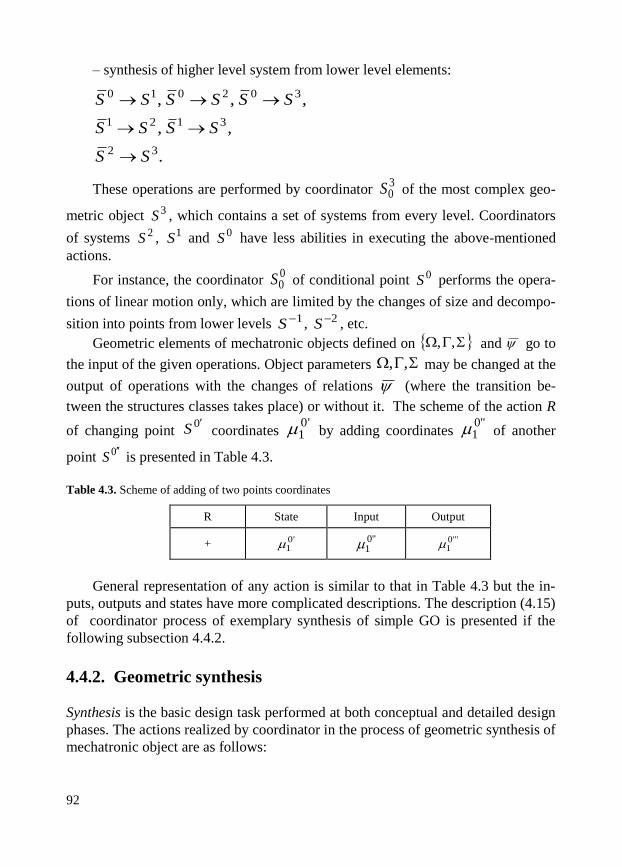
92
– synthesis of higher level system from lower level elements:
.
,,
,,,
32
3121
302010
SS
SSSS
SSSSSS
These operations are performed by coordinator 30S of the most complex geo-
metric object 3S , which contains a set of systems from every level. Coordinators
of systems 2S , 1S and 0S have less abilities in executing the above-mentioned
actions.
For instance, the coordinator 00S of conditional point 0S performs the opera-
tions of linear motion only, which are limited by the changes of size and decompo-
sition into points from lower levels 1S , 2S , etc.
Geometric elements of mechatronic objects defined on ,, and go to
the input of the given operations. Object parameters ,, may be changed at the
output of operations with the changes of relations (where the transition be-
tween the structures classes takes place) or without it. The scheme of the action R
of changing point 0S coordinates
'01 by adding coordinates
"01 of another
point 0 S is presented in Table 4.3.
Table 4.3. Scheme of adding of two points coordinates
R State Input Output
+ '01 "0
1 "'01
General representation of any action is similar to that in Table 4.3 but the in-
puts, outputs and states have more complicated descriptions. The description (4.15)
of coordinator process of exemplary synthesis of simple GO is presented if the
following subsection 4.4.2.
4.4.2. Geometric synthesis
Synthesis is the basic design task performed at both conceptual and detailed design
phases. The actions realized by coordinator in the process of geometric synthesis of
mechatronic object are as follows:

93
1. defines the constructive dimension of the resultant geometric structure of
mechatronic object (chooses the required structure class 3210 ,,, from );
2. defines kinds of changes of initial standard element of the defined structure
which are necessary to perform the constructing of the required object gmS;
3. sets the sequence of the changing actions from the above determined classes
(subsection 4.4.1);
4. performs these actions (this process corresponds to the calculations of the
resultant object gmS characteristics ,, ).
Relations between the basic geometrical structures are presented in the form of
procedures from the given classes. So, it became possible to choose a class of pro-
cedures for the synthesis of a required output object from the given input object.
The dynamics of states of input object Sgm is described with the help of dynamic
system ,o .
An example of the dynamics of the object states in the synthesis process is
given in the following Scheme 4.1. Both the structure and form of GO are continu-
ously changed. The dynamics of the process (two steps) is described by the follow-
ing reactions:
TYXCo 1&: 1111 , (4.18)
TYXCo 2&: 2222 .
t=1,
C1: X1: Y1 :
t=2,
C2: X2: Y2:
Scheme 4.1. Two states of GO synthesis process
That is, at the moment of time t=1 the basic GO is the conditional line (C1),
the input (X1) is the conditional point and the output (Y1) is a composition of these
objects. Reaction 1 corresponds to the coordinator action of type 2 (subsection
4.4.1). At the next moment t=2, the basic element C2=Y1 is the conditional line

94
constructed in the previous moment t=1, input object (X2) is another conditional
line, and the output object (Y2) is a composition of two conditional lines which is
the initial state of a conditional surface. Reaction 2 corresponds to the coordinator
action of type 3 (subsection 4.4.1).
The set of primitives, which are used in the synthesis process is presented in
Table 4.4.
Table 4.4. Set of primitives of different level systems
Levels S0 S1 S2 S3
Primitives Points parts of lines,
curves
circles, cubes,
triangles, rings
spheres, cubes, cones,
cylinders, pyramids
(3D simplex)
For instance, coordinator actions R0:CXY (where 00
1 ,..., nSSС ,
,1X , 1SY ) make it possible to synthesise the part of line 1S from
frame C of points (cubes 00
1 ,..., nSS ), when the structure type and additional infor-
mation are received from designer (Fig. 4.6). All the parameters ,, of the
part of line 1S are defined in this process as follows:
GO being synthesised S is the conditional line 1S ;
structure type ↔ line; structural connections – sides of cubes;
structural elements are conditional point 1 =0
1S – cubes;
metrical characteristic of the elements 01 = w;
another metrical characteristic of the line l = 11 = n ,0
1 is defined by the
number n of structural elements and their sizes w = 01 ;
constructive dimension of the line in its aggregated form is
= 0 0 1 0; constructive dimension of the line in its structural form is
= 0 0 0 n, etc.
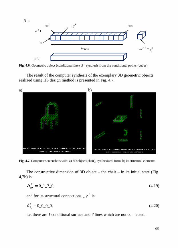
95
1S :
i=1 i=n
:
w
l=w•n
:
Fig. 4.6. Geometric object (conditional line) 1S synthesis from the conditional points (cubes)
The result of the computer synthesis of the exemplary 3D geometric objects
realized using HS design method is presented in Fig. 4.7.
a) b)
Fig. 4.7. Computer screenshots with: a) 3D object (chair), synthesized from: b) its structural elements
The constructive dimension of 3D object – the chair – in its initial state (Fig.
4,7b) is:
0_1_7_0, (4.19)
and for its structural connections is:
0_0_0_0, (4.20)
i.e. there are 1 conditional surface and 7 lines which are not connected.
1 = 01S

96
In the final state of the chair synthesis (Fig. 4.7a) there are 1 conditional sur-
face and 4 lines connected by conditional 6 points, and constructive dimensions are
as follows:
0_1_4_0 and
0_0_0_6. (4.21)
One conditional line is constructed form three initial ones. Therefore the 7
turns into 4 in the second position of numeric code which is the position of
lines in the constructive dimension code. All constructive elements of the chair
in its final state are connected by conditional points. Figs. 4.7a and 4.7b are com-
puter screenshots.
4.4.3. Motion design and deformation as analysis tasks
The tasks of mechatronic object (MO) motion design and deformations - analysis
tasks - are defined as the coordination tasks of hierarchical system standard block S (aed).
Object Sm movement in its environment
S is called a change of its inter-
connections with the elements
iS ( 1 Ii ) of environment system
S .
The change of interconnections of the elements of MO structure is
identified as deformation.
Adding of negative and positive units (elements) to the connections
with structure remaining it in the same structures class causes the effect of
structure deformation. The change of causes the external interconnec-
tions changes which are equivalent to object
So movement in its environ-
ment. The accordingly organized deformations - for instance running waves of
deformations [55] - correspond to the classes of ways of object motion coordina-
tion.
The objects mass measure is defined as the metrical characteristics ~
of system Sm state
Cc , its inputs X and outputs
Y .
Neutral element 111010 ~~,~,~~ is the length, square or
volume measure – depending on which object state (i.e. which constructive dimen-
sion ,
and connection defect ,
) is considered as C or , L .

97
Movement measures (velocity, impulse, etc.) are presented as the measures of
state changing of dynamic systems during the time unit T ,
},,,{ TTTTTT in spaces , , . Movement measures
have their directions in accordance with environment S element addresses with
regard to which the movement is considered. The general law of movement and
deformation was also presented in form of aed .
Geometric and physical values were defined in state spaces , , , T .
All calculations are carried out in these spaces with the help of numeric positional
system SL . The ways of motion design and deformation calculations depend on
the units ~ , ~
, ~
of both structure and aggregated dynamic realization .
The ways correspond to coordination strategies oooooo ,,,
for different levels of information uncertainty of coordinator.
It is possible to define different kinds of movements and deformations by in-
troducing corresponding conditions. For instance, the following relation corre-
sponds to MO physical movement (object’s coordinates changing) at time interval ttT
:
constT tt , (4.22)
where structural connections are not changed (at this time period) and in this
way structure remains in its current state. This movement is conditioned by
environment process S , which was presented in the following way:
, : TtYCX tttt &: , (4.23)
ttTttXCX tttttt &,&: ,
YXX , XYY
.
The following relation corresponds to the bio-mechanical type of movements:
constTTYX tttt )( , (4.24)
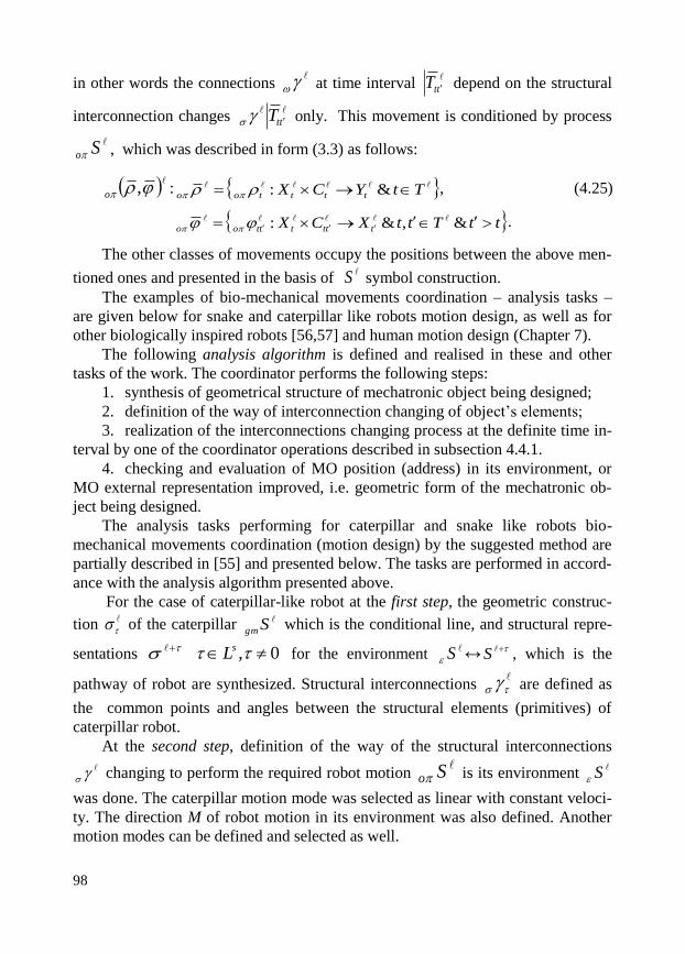
98
in other words the connections at time interval
ttT depend on the structural
interconnection changes ttT only. This movement is conditioned by process
So , which was described in form (3.3) as follows:
,o : TtYCX ttttoo &: , (4.25)
ttTttXCX ttttttoo &,&:
.
The other classes of movements occupy the positions between the above men-
tioned ones and presented in the basis of S symbol construction.
The examples of bio-mechanical movements coordination – analysis tasks –
are given below for snake and caterpillar like robots motion design, as well as for
other biologically inspired robots [56,57] and human motion design (Chapter 7).
The following analysis algorithm is defined and realised in these and other
tasks of the work. The coordinator performs the following steps:
1. synthesis of geometrical structure of mechatronic object being designed;
2. definition of the way of interconnection changing of object’s elements;
3. realization of the interconnections changing process at the definite time in-
terval by one of the coordinator operations described in subsection 4.4.1.
4. checking and evaluation of MO position (address) in its environment, or
MO external representation improved, i.e. geometric form of the mechatronic ob-
ject being designed.
The analysis tasks performing for caterpillar and snake like robots bio-
mechanical movements coordination (motion design) by the suggested method are
partially described in [55] and presented below. The tasks are performed in accord-
ance with the analysis algorithm presented above.
For the case of caterpillar-like robot at the first step, the geometric construc-
tion of the caterpillar Sgm
which is the conditional line, and structural repre-
sentations
0, sL for the environment S ↔ S , which is the
pathway of robot are synthesized. Structural interconnections are defined as
the common points and angles between the structural elements (primitives) of
caterpillar robot.
At the second step, definition of the way of the structural interconnections
changing to perform the required robot motion So is its environment
S
was done. The caterpillar motion mode was selected as linear with constant veloci-
ty. The direction M of robot motion in its environment was also defined. Another
motion modes can be defined and selected as well.

99
Fig. 4.8. Caterpillar robot motion, where: S – robot body displacement during one motion cycle;
5,4 – structural connections of 4 and 5 elements of the body, M – direction of the motion
At the third step, the consecutive change of structural interconnections (an-
gles) in the way defined by coordinator at the second algorithm step leads to the
whole robot movements in its environment S ↔S (Fig. 4.8). The change of
angles ,i , sLi , from their maximum value to 0 during one motion circle
causes displacement equal to S of the robot body.
At the fourth step, the checking and evaluation of the changes of the both posi-
tion and form, i.e. external representation of caterpillar robot Sgm in its envi-
ronent S are executed in parallel with the actions of the third algorithm step.
a) b)
Fig. 4.9. Two states of motion design of caterpillar like robot movements, M – motion direction
S
1
4,5
1
1
S M
x y
z
x y
z
M M

100
The result of computer performing of motion design task for the caterpillar ro-
bot is presented in Figure 4.9. The figure is a computer screen-short obtained.
Motion design of snake like robot is the another exemplary analysis task. The
mechanism of snake like robot motion is a combined mechanism of transverse and
lengthwise waves of structural interconnection change spreading in the snake body.
For lengthwise waves of deformation the interconnections volume
changes for relative elements i, and continuous interconnections
transfer (i=i+1 or i=i-1) depending on the direction of the mass being transferred
take place (Fig. 4.10). The strength of the structural connections is graphically
illustrated by their volumes. Robot body displacement during one motion cycle is
equal to Motion design of snake like robot is performed according to the
analysis algorithm given above.
Fig. 4.10. Construction of a body of snake-like robot being in motion, where 1'1
tS is the new position
of the first element (head) in the moment of time t’, M – direction of the motion
At the first step of the analysis task, geometric construction of biomech-
atronic object – snake like robot – is synthesized in the form of conditional
line built from conditional points – cubes (Fig. 4.10). Interconnections of
conditional points i and j are their common edges and angles. The snake robot con-
struction at initial t moment is in the state presented in Figure 4.10.
At the second and the third algorithm steps, definition of the way of the snake
robot structural interconnections changing to perform the required robot mo-
tion is its environment was done. The direction M of robot motion in
its environment was also defined. After that, the coordination of the snake motion
process was realized in the following way. The character of snake motion is based
on the principle that each part of the snake body goes the same way in the motion
,i
))((3 ti
.S
m
Sm
ji,
tm
So
S
11'tS
1
1
tS 1
2
tS
1nS 1
1
nS
t2,1
M
t'2,1
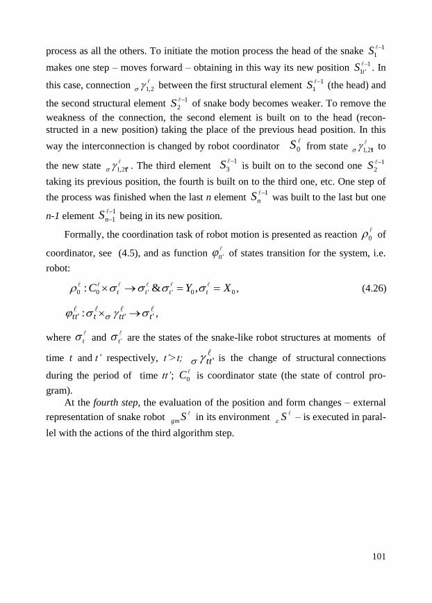
101
process as all the others. To initiate the motion process the head of the snake
makes one step – moves forward – obtaining in this way its new position . In
this case, connection between the first structural element (the head) and
the second structural element of snake body becomes weaker. To remove the
weakness of the connection, the second element is built on to the head (recon-
structed in a new position) taking the place of the previous head position. In this
way the interconnection is changed by robot coordinator from state to
the new state . The third element is built on to the second one
taking its previous position, the fourth is built on to the third one, etc. One step of
the process was finished when the last n element was built to the last but one
n-1 element being in its new position.
Formally, the coordination task of robot motion is presented as reaction of
coordinator, see (4.5), and as function of states transition for the system, i.e.
robot:
, (4.26)
,
where and are the states of the snake-like robot structures at moments of
time t and t’ respectively, t’>t; is the change of structural connections
during the period of time tt’; is coordinator state (the state of control pro-
gram).
At the fourth step, the evaluation of the position and form changes – external
representation of snake robot in its environment – is executed in paral-
lel with the actions of the third algorithm step.
1
1
S1
'1
tS
2,1
1
1
S
1
2
S
0S
t2,1
t'2,1
1
3
S 1
2
S
1nS
1
1
nS
0
'tt
00''00 ,&: XYC tttt
''' : tttttt
t
't
'tt
0C
Sgm
S

102
a) b)
Fig. 4.11. Computer screen shorts obtained in the process of the snake-like robot motion design
In the program realization of snake robot motion design, the coordinator ,
which is realized as the main control program, controls the interconnections
change of the body elements and reconstructs the elements consecutively in
their new positions. The wave of the interconnections change runs from the head
to the last structural element . This process of change causes the
shake robot motion in the opposite direction M. Two states of the body construc-
tion of the snake robot being in motion are given in Fig. 4.11.
So, in the case of motion design of caterpillar and snake like robots we deal
with two kinds of geometric design (analysis) processes – deformation (in the low-
er level structure of the biomechatronic object) and motion, i.e. its dynamics in the
structure of the environment.
The results obtained in performing the given tasks have a general character
and may be used in an abstract motion design of hierarchical systems. The con-
ducted researches show that the HS design method proposed in this book can be
used both in the conceptual and detailed design tasks of mechatronic objects mo-
tion, i.e. coordination of biomechanical movements, and deformation analysis of
the objects constructed.
0S
ji,
1S
1
1
S1
nS ji,
x y
z
x y
z

103
Preliminary conclusions
The HS design method of mechatronic objects (MO) has been described in this
Chapter 4.
First, the steps of the method realization were defined.
After that, in accordance with the method steps, the basic geometric elements
of MO were presented in the hierarchical form. The results of this presentation
are conditional point, line, surface and 3D object.
Later, the geometrical and numeric characteristics of MO were introduced.
The main numeric characteristics, i.e. constructive dimension and connections
defect, are presented in the numeric positional code.
Next, coordinator procedures of mechatronic systems design were defined.
Algorithms of hierarchical objects synthesis and analysis were presented.
Finally, the exemplary computer realizations of the method for solving the
basic design tasks were described: synthesis of 3D objects and analysis – design of
caterpillar and snake like robots movements. Program modules have been written
in Pascal language and work in the frames of standard operation systems. The role
of coordinator is performed by the main control program unit, which realizes the
functions of coordinator selection stratum, i.e. solves synthesis and analysis design
tasks.
The computer realization shows, that the method has the main advantages of
the wide spread technologies of geometric design. At the same time hierarchical
representation of geometric elements of MO is free from certain drawbacks of the
known methods.

104
5. CONCEPTUAL DESIGN
OF BIOMECHATRONIC SURGICAL
ROBOT SYSTEM
The Chapter presents the application of Hierarchical System (HS) technology in
the task of conceptual design of biomechatronic Surgical Robot System (SRS).
This task is topical for the systems of Computer Aided Design (CAD) and
processes of conceptual mechatronic design in particular [1,58]. In design process
of biomechatronic systems we deal with objects which contain connected
mechanical, electromechanical, biological, electronic, computer and human-
computer subsystems. It is important to define the common conceptual model
which will describe all the above mentioned systems of biomechatronic SRS being
designed in common formal basis.
The model must also be coordinated with numerical and geometrical systems,
i.e. the traditional forms of information representation in mechatronics. The
theoretical basis of design process in agreement with these requirements must be a
hierarchical construction connecting any level unit with its lower and higher levels.
Mathematical and cybernetic theories based on the set theory are incoherent with
the above design requirements since the set theory describes one-level outlook.
So, the coordination technology of Hierarchical System with its standard block
aed described in Chapters 3 and 4 is applied in this Chapter as a theoretical basis
for the performing of conceptual design task of biomechtronic SR system. Accord-
ing to the definitions – given above in the Introduction and Chapter 1 – Conceptual
Design (CD) is recognized in this book as a process of creation of the systemic
model of the object being designed on the early phase of its life cycle which is
before the Detailed design (DD) phase of object’s concrete mathematical model
creation and numeric calculations realization. In the frames of the HS method pro-
posed, to create conceptual model for design of biomechatronic object, e.g. Surgi-
cal Robot System (SRS) in our case, means to define SR system structure; its dy-
namic representation as the unit in its environment; SRS environment, its process
and SRS-Environment interactions; SR system coordinator and its design and con-
trol processes; processes executed by SRS subsystems and general SRS process.

105
Therefore, the conceptual model of biomechatronic surgical robot system (SRS)
presented in aed formal basis of HS is given first in this Chapter. The exemplary
tasks performed by SRS subsystems are described after that in frames of HS tech-
nology as well.
5.1. Conceptual formal model of surgical robot system
SR systems, such as commercial ROBODOC system [59] (Integrated Surgical
Systems, CA, USA), have been widely used recently in TKA (Total Knee Artho-
plasty) surgery [60]. Total knee arthroplasty is one of the major type of surgery for
people with severe knee damage to relieve the pain and disability of cartilage inju-
ry, osteoarthritis, rheumatoid arthritis, or psoriatic arthritis [61, 62]. Due to the
increasing aging population recently, the TKA surgery has been grown rapidly in
the world. The main surgical procedure of the TKA is removing damaged cartilage
and bones from the surface of the knee joint and replacing them with femoral and
tibia components of TKA implant (Fig. 5.4). In order for the surgery to be success-
ful and the longevity of the implant to be achieved, the accurate bone cutting and
implant alignment along the preoperative planning are required. Conventional sur-
gical planning is performed basing on 2D plane x-rays and bone cutting is per-
formed manually using electric saw, which strongly relies on a surgeon’s experi-
ence. Even for a skilled surgeon, the implant alignment with respect to the bone in
frontal plane is a very complicated task. So it is necessary to achieve excellent
implant alignment and bone cutting by utilizing Computer Tomography (CT) based
3D planning and robot assisted accurate bone cutting. The minimal invasive sur-
gery (MIS) in the knee arthroplasty has been increased since MIS can improve the
surgical outcomes such as the recovery time and hospital stay by reducing the inci-
sion in surgery.
Recently, commercially available computer-aided surgical robot systems have
been introduced to enable surgeons to improve the accuracy of cutting and align-
ment in knee and hip arthroplasty. The surgical robot systems could be classified
into semi-active type and active type. The semi-active robot systems such as the
MAKOPLASTY® system (MAKO Surgical Co, Fort Luderdale, FL, USA [63]) or
ACROBOT Sculptor (The Acrobot Co., Elstree, UK [64]) provide a surgeon active
control over the robot by hands.
These robot systems also protect the cutting tool from moving out of the
planned cutting space by actively blocking the robot arm attached to the cutting
tool when the surgeon executes the bone cutting process. The active robot systems
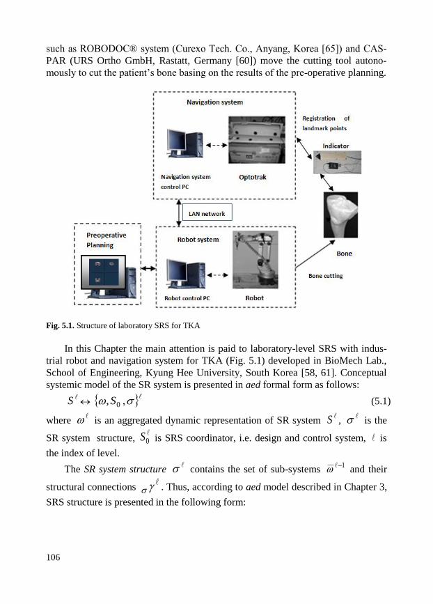
106
such as ROBODOC® system (Curexo Tech. Co., Anyang, Korea [65]) and CAS-
PAR (URS Ortho GmbH, Rastatt, Germany [60]) move the cutting tool autono-
mously to cut the patient’s bone basing on the results of the pre-operative planning.
Fig. 5.1. Structure of laboratory SRS for TKA
In this Chapter the main attention is paid to laboratory-level SRS with indus-
trial robot and navigation system for TKA (Fig. 5.1) developed in BioMech Lab.,
School of Engineering, Kyung Hee University, South Korea [58, 61]. Conceptual
systemic model of the SR system is presented in aed formal form as follows:
(5.1)
where is an aggregated dynamic representation of SR system , is the
SR system structure, is SRS coordinator, i.e. design and control system, is
the index of level.
The SR system structure contains the set of sub-systems and their
structural connections . Thus, according to aed model described in Chapter 3,
SRS structure is presented in the following form:
S 0,S
S 0S
1

107
(5.2)
where the SRS subsystems presented in aggregated dynamic form are
: robot system (RS);
: pre-operative planning system (PP);
: navigation system (NS);
: computer control system (CCS).
CCS is presented in the form of SRS coordinator (Fig. 5.7) and contains con-
trol PC of robot, control units of pre-operative planning and navigation subsys-
tems, and communication program developed to integrate the SRS subsystems.
Therefore, CCS 1
4 partially plays the role of SRS coordinator
0S which per-
forms design and control functions of SRS.
In their turn, each subsystem has its own structural elements – lower level
1 subsystems. For the robot mechatronic subsystem RS 1
1 they are manipu-
lator 2
1,1 (mechanical), servomotors
22,1 (electromechanical), cutting machine
23,1 (pneumatic) and its own control system
24,1 (computer). All the subsys-
tems are connected by their structural connections 2 . For instance, cutting
machine 2
3,1 and manipulator
21,1 are connected by end effector
23,1 of
robot. By analogy, the higher level subsystems 1 are connected by their com-
mon parts – structural connections 1 – that are the elements of lower levels.
For instance, navigation system 1
3 and robot
11 are connected by their com-
mon element – communication program of computer control system 1
3,1 =
24,1 =
24,3 , where
24,1 is dynamic representation of the control program being
the subsystem of robot 1
1 , and
24,3 the one of the control program being the
subsystem of the navigation system 1
3 .
Aggregated dynamic realizations 1 , i.e. dynamic models
1),( i of
SRS subsystems 1S , are formed after the definition of subsystems’ inputs-
outputs concerning each particular sub-process they execute. Thus, for the naviga-
tion system 1
3 concerning its registration process of bone and robot, the input
11
11
21
3
14
}},,{,{ 10
S

108
13X is optic signal received by Optotrak 3020 cameras system (Northern Digital
Inc., Canada) and the output 1
3Y is the robot instrument and real bone coordinates
written on control PC. State 1
3C in this case is the stage of registration process
completeness. This process is of informational nature. As for the robot subsystem 1
1 , concerning its mechanical process of cutting instrument motion, the aggre-
gated realization 21,1 presented in ),( form at the conceptual design (CD)
phase (Fig. 1.2, Chapter 1) can be transformed to differential equations [58] of
inverse kinematics at the detailed design (DD) phase:
xqJq )(
(5.3)
Equation (5.3) connects robot joints velocities q as the output parameter 1
1Y
with velocities x of robot cutting instrument as input 1
1X , where J is the pseu-
do inverse of the Jacobian matrix.
Object So (SR system), its environment
S , their processes So and
S (TKA and SRS control) and coordinator 0S (design and control system)
create a general biomechatronic SR system for TKA.
Environment S of the SR system has its own structure and contains:
1 : bone (biological system),
2 : surgeon, who communicates with SRS via video information,
registration and cutting motion planning system (human-computer system),
3 : other biomechatronic systems being in interaction with SRS (e.g. com-
puter tomography (CT) system, which supply PP subsystem of SRS with the CT
images of bone),
4 : implant producing system (bioengineering system),
5 : higher level coordinator (higher level design and control system).
Thus the control interactions between surgeon (operator) 2 and SR system
are realized through obtaining video information of bone, checking the cutting path
and robot cutting motion planning. In their turn, the interactions between robot
cutting instrument and bone 1 are the executive interactions between SR system
and its environment.

109
The immediate input X for the SR system (which is at the same time the
output YX of the environment of SR system) are control actions produced
by surgeon and the inputs generated by other environment systems, e.g. inserted
implant presented by 4 . The output Y of the SR system is the cutting bone. The
output of the SR system S is at the same time the input X
Y of the envi-
ronment. According to the relations established for the elements of ),( model –
see Table 3.1, Chapter 3 – the states iC of SR system
S are the inputs of TKA
surgical process.
Dynamic representation of SR system and its subsystems are constructed
in ),( form (3.2) by the inputs X , states C and outputs Y mentioned above.
For example, in the case of description of robot end effector motion, the dynamic
representation which is given in ),( form at CD phase can be transformed at
DD phase to the states space equations as follows:
BuAxx (5.4)
Cxy .
First state equation in system (5.4) corresponds to the state transition function
in (3.2) and the second output equation corresponds to the reaction . Vectors
x, y, u and matrices A, B, C must be predefined. In the case of robot end effecter
motion the elements of states vector x=[x1 x2 x3]T are the displacement x1, velocity
x2 and acceleration x3.
SR TKA system process So is part of higher-level process
1S in SRS
environment S which contains biomechatronic system of higher level – general
design&control system including surgeon, person being operated, other biomecha-
tronic systems being in interaction with SRS (e.g. CT system and implant produc-
tion system).
This process contains:
1S : VM of bone and implant graphic image forming (by PP system),
2S : real bone image and robot instrument location registration (by NS),
3S : VM matching to real bone model – bone image,
4S : cutting path forming in PP and transforming to coordinates system of RS,

110
5S : allocation of robot instrument in the registration points by surgeon using
control haptic device, and definition of robot joints angels control law by solving
inverse kinematics problem,
6S : sending control signal to AS3 robot system,
7S : AS3 robot motion and end effector (pneumatic milling instrument) dis-
placement,
8S : bone cutting (or milling) and implant inserting.
Fig. 5.2. Stacking process of the bone model creation from CT bone images a) and b), i.e. slices.
For instance, 1S process of the bone virtual model – bone image – creation
is described at conceptual design (CD) phase as follows. The model of a bone bio-
logical subsystem of general biomechatronic SR system is constructed in virtual
space from computer tomography (CT) images, i.e. bone slices (Fig. 5.2). The
process of the bone model creation is called stacking.
The stacking process 1S (Fig. 5.2) is formally described at the phase of CD
in the form of reaction of dynamic system :),(
(5.5)
where initial slice (or composition of previously connected slices) is recognized as
state C1, at step 1, slice to be added to the initial one is recognized as input X1, and
the composition of both the connected initial and input slices is recognized as out-
put Y1. Output Y1 becomes state C2 at the next step of stacking process.
Virtual bone structure is presented at CD phase according to aed model in the
form:
(5.6) },{ 1
}1&:{ 1111 TYXC

111
where is a set of bone CT slices, and are their structural interconnec-
tions, i.e. common surface of neighboring slices.
The general synthesis process of the virtual bone construction is formally de-
scribed as coordinator task according to the HS design method step 4 (See Chapter
4) in form of (4.4) as follows:
(5.7)
a) b)
Fig. 5.3. a) top view of tibia bone in matching 3S process, where red and yellow triangles represent
three corresponding points from PP and robot coordinate systems respectively, b) AS3 Samsung robot
system, man-operator and fixed bone being operated
Because of the fact that pre-operative planning (PP) system and the robot sys-
tem (RS) have their own coordinate systems, registration process 2S is required
to transfer information to RS coordinates about bone cutting trajectory represented
in coordinates of PP system. A transformation matrix between two coordinate sys-
tems is calculated with three corresponding points – represented by red and yellow
triangles – from each coordinate system where each point has the same location in
both coordinates (see Fig. 5.3). After that, the cutting trajectory calculated in the
pre-operative planning system is transformed into the cutting trajectory in the co-
ordinates of the robot system. This process 3S is called matching.
1
},{: 10S

112
Human-computer PP system Optotrak NS system AS3 robot RS system Haptic device&surgeon
Pre-operating planning Registration Bone cutting Implant inserting
Fig. 5.4. Several steps of SRS TKA process So – bone cutting and implant inserting – executed by
SRS subsystems 1 and
After performing a matching process a bone cutting and implant inserting pro-
cesses … are realized (see Fig. 5.4). To move the milling tool along the
cutting trajectory, the values of the robot joint angles at each time step are calculat-
ed for AS3 robot system (Rockwell Samsung Automation Inc., Korea) by per-
forming the inverse kinematics task. For the accuracy of the inverse kinematics
analysis, first, each length of the robot link from the manufacture specification is
analyzed and calibrated to match the pre-defined known positions and orientations
of the end effecter of the robot system by trial-end errors. Then, the exact trans-
formation of the robot links from the origin coordinate to the robot end effecter is
reconstructed for the calculation of the joint angle profiles for given bone cutting
trajectory input.
Pre-operative planning (PP) system has to reconstruct the 3D model of a bone,
choose an implant model, align the bone and the implant models, and calculate the
cutting trajectory of the tools to allow the appropriate location and orientation of
the implant with respect to the tibia bone. PP system connects the robot and virtual
bone spaces to calculate a bone cutting trajectory. Processes 1S and
3S are
associated with PP human-computer system, 2S and
5S – with navigation sys-
tem (NS), and 6S …
8S processes are associated with robot system (RS) (Figs.
5.1, 5.3b and 5.4). NS registers 3D positions of real bone and AS3 robot instrument
by Optotrak 3020 cameras system (Northern Digital Inc., Canada) to transfer the
cutting trajectory being planned to robot system. NS also transforms the bone co-
ordinates system in real space to the coordinate system in virtual space in PP sys-
tem. The trajectory calculated in PP is transformed into coordinates of robot sys-
tem. The control signals to robot joints are generated by Robot Control System
3S
8S
Virtual bone
Real bone

113
and Multi Motion Controller (Rockwell Samsung Automation Inc., Korea) [58]
to realize the cutting trajectory. The inverse kinematic task is performed before it.
NS and RS are coordinated by different control PC computers connected by LAN
network (Fig. 5.1) with correspondent communication program [61] developed to
integrate the systems.
7S is realized by electromechanical subsystems (AS3 robot servomotors) of
the general biomechatronics SR system, 1S –
4S are realized by video-
information and computer subsystems, and 8S is realized by pneumatic and me-
chanical ones. The general process is composed by sub-processes S , executed
by the general biomechatronic system, which includes the SR system So and its
environment S . All the sub-processes
iS are realized by different nature sub-
systems of the general SR biomechatronic system.
So, all the subsystems of general biomechatronic SR system, i.e. mechanical
(AS3 manipulator 2
11
S , haptic system), electromechanical (servomotor 2
12
S ),
pneumatic (cutting-milling instrument 2
13
S ), computer-electronic (navigation 1
3
S
and control system 1
4
S ), human-computer (surgeon and preregistration system)
have their aggregated dynamic and structural descriptions. The sub-
processes iS are also presented at CD phase in , form (3.5), see Chapter 3.
All the connected descriptions of the subsystems S and processes S are pre-
sented in the informational resources (data bases) of the coordinator which per-
forms the design and control processes, connecting in this way structure and
the functional dynamic realization of the SRS being coordinated.
Coordinator 0S in our case is realized in the form of human-computer de-
sign&control system of the SRS, which maintains its functional modes by surgeon
and control system and realizes the design process by higher level computer aided
design (CAD) system if necessary. All metrical characteristics of SR subsystems
and processes are presented at CD phase in the form of numeric positional systems
Ls (see Chapters 3,4).

114
5.2. Realization of coordination – design and control – tasks
Coordinator 0S
tasks in control process
0S of SRS are performed by human-
computer system, i.e. surgeon communicating with servers and robot. The main
control tasks, i.e. functions, are indicated in the graphic user interface (GUI) win-
dow of control program (Fig. 5.5) developed in Biomechanics Lab., School of En-
gineering, Kyung Hee University, Yongin, Korea [61]. The main control processes
are: 1) bone fixation and its position checking 01 S , 2) registration of robot posi-
tion 02 S , 3) registration of real-virtual bone relations
03 S , 4) calculation of the
cutting path and realization of a bone cutting 04 S .
Fig. 5.5. GUI window of control program of SRS which performs TKA process S
All the control processes have their sub-processes indicated by correspondent
buttons on the GUI control panel. 01 S control process of bone fixation and its position checking contains the
sub-processes performed by surgeon:

115
1.1. bone fixation and allocation according to the device position;
1.2. moving robot to the working area and checking the position of the robot
end effecter; 02 S process of robot position registration contains the sub-processes of:
2.1. robot displacements using haptic device and getting 3 registration points
coordinates and joint angles by Multi Motion Controller (MMC) – data collecting,
2.2. registration of 3 registration points by Optotrak – collecting coordinates in
another coordinate system,
2.3. loading of the data collected to SRS control program,
2.4. calculating the coordinates matrix transform – setting the relation of coor-
dinate systems of Optotrak and AS3 robot,
2.5. checking the matrix transform – choosing any control point and compari-
son of the coordinates values; 03 S control process of registration of real-virtual bone relations contains the
sub-processes of:
3.1. loading data of 3 registration points of virtual bone from GUI to program,
3.2. collecting and loading data of real bone using Optotrak cameras,
3.3. performing matching algorithm by calculating matrix transformation and
setting relation between real and virtual bones,
3.4. checking of matrix transformation; 04 S control process of calculation of cutting path and bone cutting realiza-
tion contains the sub-processes of:
4.1 cutting path loading from PP system – planning program,
4.2. calculation of robot end effecter cutting path by performing matrix trans-
formations and inverse kinematics task,
4.3. realization of cutting – loading of manipulator angular change data to con-
trol MMC unit and execution of the event.
Formally, SRS control processes are described at CD phase in 0),( form
of coordinator functions (see Chapter 3) after definition of the states tC0 , inputs
tX 0 and outputs
tY0 of control subsystems:
TtYXC tttt &::, 000000 , (5.8)
ttTttCXC tttttto &,&: 00000 .
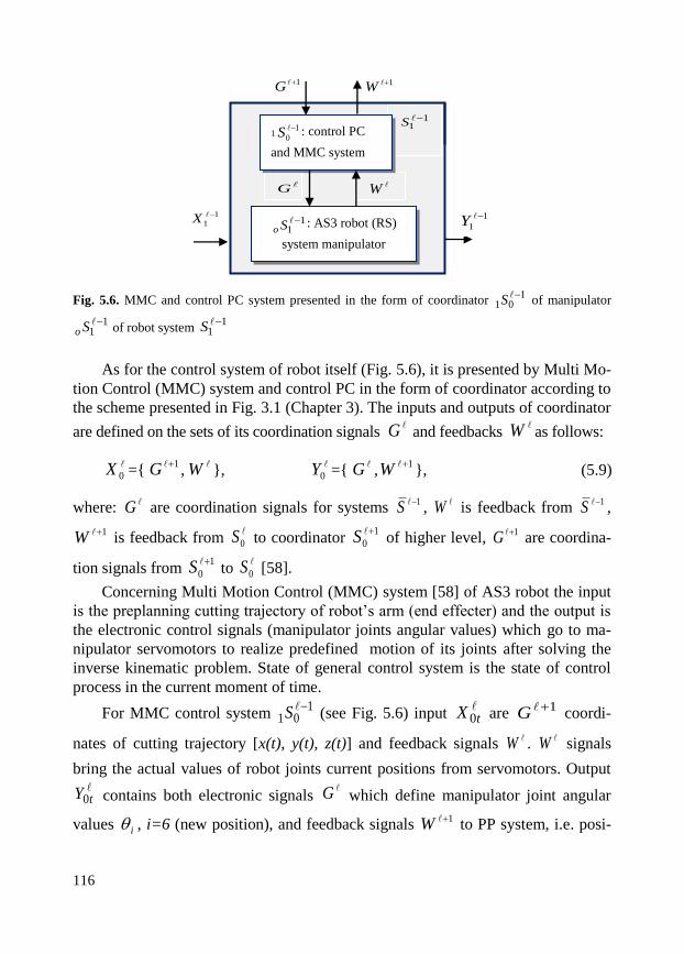
116
Fig. 5.6. MMC and control PC system presented in the form of coordinator 1
01S of manipulator
11So of robot system
11S
As for the control system of robot itself (Fig. 5.6), it is presented by Multi Mo-
tion Control (MMC) system and control PC in the form of coordinator according to
the scheme presented in Fig. 3.1 (Chapter 3). The inputs and outputs of coordinator
are defined on the sets of its coordination signals and feedbacks as follows:
={ , }, ={ , }, (5.9)
where: G are coordination signals for systems
1S , W is feedback from
1S ,
1W is feedback from 0S to coordinator
1
0
S of higher level,
1G are coordina-
tion signals from 1
0
S to
0S
[58].
Concerning Multi Motion Control (MMC) system [58] of AS3 robot the input
is the preplanning cutting trajectory of robot’s arm (end effecter) and the output is
the electronic control signals (manipulator joints angular values) which go to ma-
nipulator servomotors to realize predefined motion of its joints after solving the
inverse kinematic problem. State of general control system is the state of control
process in the current moment of time.
For MMC control system 1
01S (see Fig. 5.6) input
tX 0
are 1G
coordi-
nates of cutting trajectory [x(t), y(t), z(t)] and feedback signals W .
W signals
bring the actual values of robot joints current positions from servomotors. Output tY0 contains both electronic signals
G which define manipulator joint angular
values i , i=6 (new position), and feedback signals 1W to PP system, i.e. posi-
G W
0X 1G W
0Y G 1W
11S
G
W
11
0
S : control PC
and MMC system
11So
: AS3 robot (RS)
system manipulator
1G 1W
1
1
X
1
1
Y
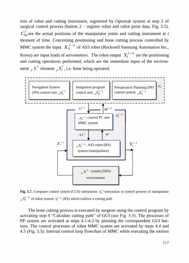
117
tion of robot and cutting instrument, registered by Optotrak system at step 2 of
surgical control process (button 2 – register robot and robot point data, Fig. 5.5). tC0 are the actual positions of the manipulator joints and cutting instrument at t
moment of time. Concerning positioning and bone cutting process controlled by
MMC system the input 1
1X of AS3 robot (Rockwell Samsung Automation Inc.,
Korea) are input loads of servomotors. The robot output
1
1Y are the positioning
and cutting operations performed, which are the immediate input of the environ-
ment S element
iS , i.e. bone being operated.
Fig. 5.7. Computer control system (CCS) subsystems 1
0
S interaction in control process of manipulator
11So of robot system 1
1S (RS) which realizes a cutting path
The bone cutting process is executed by surgeon using the control program by
activating step 4 “Calculate cutting path” of GUI (see Fig. 5.5). The processes of
PP system are activated at steps 4.1-4.3 by pressing the correspondent GUI but-
tons. The control processes of robot MMC system are activated by steps 4.4 and
4.5 (Fig. 5.5). Internal control loop flowchart of MMC while executing the motion
0S
Preoperative Planning (PP)
control system 102S
Navigation System
(NS) control unit 103S
Integration program
control unit 104S
11S
G
W
101S : control PC and
MMC system
11So
: AS3 robot (RS)
system (manipulator)
1G 1W
1
1
X
1
1
Y
S : system (SRS)
environment

118
process of robot end effecter along the cutting trajectory is given in Fig.5.8.
The control loop flowchart is presented in the form of coordination process 1
01S
of coordinator 1
01S (MMC connected with control PC, see. Figs. 5.6 and 5.7) and
contains the sub-processes 1
01iS (Fig. 5.8).
Fig. 5.8. a) internal control loop flowchart of coordinator 1
01S – sub-processes
101iS of Multi
Motion Controller (MMC), and b) manipulator – AS3 robot being controlled
Control signals of AS3 robot manipulator (Figs. 5.7 and 5.8) are formed as a
result of inverse kinematic task performing and calculation of robot’s joints angu-
lar change after consequent placing of end effecter of robot to the positions of 3
registration points. The placement is realizes by operator (surgeon) using haptic
device connected with manipulator via robot’s control system – man-machine
mechatronic subsystem.
One of the functions of control PCs of coordination system is the commands
forming and control of each subsystem while executing general surgical process,
e.g. for Navigation System (NS), it is control of bone registration process, for Ro-
bot System (RS) – control of manipulator motion along the predefined cutting path
while executing cutting-milling process. Other functions include creation of virtual
bone and real bone images, obtaining registration points coordinates, matching,
cutting path forming according to the shape of implant, etc.
119
Coordinator 0S
tasks in the design process, realized by higher level SRS de-
sign system, are distributed on the coordinator’s strata: selection, learning and self-
organization. The design process realized by SRS coordinator correspond to the
general HS design method performance described in Chapter 4 and Section 3.2 of
Chapter 3.
On the selection stratum at Tt moment of time, predicting the environment
systems states for moment tt ' , coordinator defines correspondent inputs and
outputs of SRS system being designed and creates , models of SRS and its
process using the obtained predictions. After that, coordinator selects such states of
subsystems and their interactions which correspond to the standard state (required
for 't moment of time) of SRS system S , i.e. performs the task of structure
synthesis of the SRS being designed. Synthesis task – described in Chapter 4 – is
performed by SRS coordinator realizing its coordination strategies at both concep-
tual (CD) and detailed (DD) design phases. Coordination strategies realized on the
selection stratum of SRS coordinator are described in aed general form (3.38) in
Section 3.2.1.
The change of coordination strategies and SRS coordinator states is executed
on the learning and self-organization strata which are described by functions of
states transition 0o and
0o given in (3.39) form in Section 3.2.1. All metric
characteristics of SRS sub-systems being coordinated – designed and controlled
– and the most significant geometrical signs are defined in the frames of aed for-
mal model of HS in codes of numeric positional system SL , and presented in
(3.64) and (4.9-4.14) forms in Sections 3.2 and 4.2 respectively.
Preliminary conclusion
The conceptual model of SRS biomechatronic system presented in aed theoretical
basis of hierarchical systems for the design and control technology realization is
briefly presented in the Chapter. In comparison with models of mathematics and
artificial intelligence the proposed SRS formal model contains connected descrip-
tions of the biomechtronic system structure, its aggregated dynamic representation
as a unit in its environment and SRS environment model. All the descriptions are
connected by the coordinator which performs the design and control tasks on its
strata. Exemplary control loop of robot system (RS) coordinator is presented in the
Chapter in the form of Multi Motion Controller (MMC) which realizes coordina-
tion of AS3 robot notion. Computer control system (CCS) is presented in the form
of SRS coordinator, and CCS subsystems interaction in control process is revealed.
Model of SRS design system is given in the form of coordinator of higher level

120
which performs the design tasks on its strata: selection, learning and self- organiza-
tion. The conceptual SRS model presented in this chapter is coordinated with tradi-
tional systems of information presentation in biomechatronics – numeric and geo-
metrical forms (see Chapter 4). Aed technology of HS is also coordinated with
general requirements of design and control systems (see Chapter 1), considers the
elements of SRS conceptual model as well as connected SRS subsystems of differ-
ent nature – mechanical, electromechanical, electronic, human-computer, biologi-
cal – in common aed theoretical basis. It brings new possibilities in creating of a
formal language for conceptual design of surgical robots and other biomechatronic
systems.
Besides, the proposed conceptual model facilitates considerably the transfer
from the conceptual design phase to the detailed design phase in the mechatronic
object’s life cycle. The presentation of the conceptual model elements in the form
of the dynamic systems ),( – which are the generalization of mathematical
models (DE, automata, algebra systems [9.10]) – turns the transfer algorithm to the
detailed design phase into the concretization process of the conceptual ),(
models. It allows the efficiency of the design processes of the biomechatronic sys-
tems to be enhanced.
121
6. CONCEPTUAL MODEL
OF BIOLOGICALLY INSPIRED ROBOT
In this Chapter, a conceptual model for design of biologically inspired robot –
Bioloid Dinosaur robot [66] – is presented. Design process of robots – industrial,
universal, biologically inspired, etc. [56, 67–71, 141] – in general product life cir-
cle (see Fig. 1.2) contains several phases [1], similar to other engineering objects.
The first conceptual design phase is very important, because the main design con-
cept is generated and evaluated at this phase. According to the Hierarchical Sys-
tems (HS) technology described above (see Chapters 3,4), to create a conceptual
model of robot being designed it is necessary to take into account its several levels:
structure of robot (lower level), its aggregated dynamic representation as a unit in
environment (current level), the environment construction and technology (higher
level) and robot coordinator, i.e. robot design and control system. Therefore, a
conceptual model of Dinosaur robot in formal basis of HS technology is given first
in the Chapter. Examples of conceptual descriptions of assembly design and robot
motion design are presented after that.
6.1. Conceptual model of dinosaur robot
Conceptual model of Bioloid Dinosaur robot is presented in the frames of HS theo-
retical basis as follows:
S }, { 0 S , (6.1)
where is aggregated dynamic realisation, which represents the robot as a unit
in its environment, is structure of Dinosaur robot,
0S is coordinator which
connects with and in this way performs the design tasks, is index of level.

122
Structure of Dinosaur Bioloid robot is defined in the form of (3.14) – see
Chapter 3 – and contains aggregated representations of lower level elements (head
16 , arm
15 , body
14 , leg
13 , tail
12 , foot
11 ) and their con-
nections – the joints, see Figure 6.1.
Fig. 6.1. Structure of Dinosaur robot, 1i are structural elements,
5,4 is structural connection
of 14 and 1
5 robot elements
For example, common part of the arm 1
5 and the body 1
4 is their
structural connection, i.e. shoulder
5,4 which is the structural element of a low-
er level of Dinosaur robot. The shoulder is constructed from servo motor Dy-
manixel AX-12 [66] presented in Figure 6.3. Being the electromechanical subsys-
tem of robot mechatronic system the servo motor is describe in ),( form at the
Conceptual Design phase. ),( conceptual description is transformed to State
Space equations at the Detailed Design phase (Fig. 6.2) and can be concretized and
presented in the following form (6.2):
11
12
13
14
15
15,4
1
6

123
(6.2)
Fig. 6.2. Conceptual model transformation at the design phases
In this case first state equation of (6.2) corresponds to function, and output
equation corresponds to reaction of ),( representation. State space equa-
tions (6.2) can be transformed at DD phase to the following transfer function (6.3)
if necessary:
biama
i
a
m
KKRsJJLs
K
se
ssG
2)(
)()(
(6.3)
The meaning of the variables given in (6.2), (6.3) and Figure 6.3.are explained
below.
a) b)
Fig. 6.3. Dymanixel AX servo motor a), and its equivalent electro-mechanical scheme b)
ERi
B
K
B
K
R
K
R
L
ix
am
aaa
a
m
a
0
1
010
m
aiy
Conceptual model
),(
State space model:
BuAxx
Cxy
Conceptual Design – phase 2 Detailed Design – phase 3

124
In Figure 6.3b and equations (6.2) and (6.3), ia is armature current, La is arma-
ture inductance, Ra is armature resistance, Va(t) is input voltage, Eb is back emf, Kb
is voltage constant, TL is load torque, Tm is motor torque, θm, ωm are motor angular
change and velocity respectively, Ki is moment constant, J is motor moment of
inertia, B is friction constant, K is a constant.
Coordinator 0S of robot
So is presented in the form of (3.15) (see Section
3.1) and controls the process of robot motion on its strata of selection, learning and
self-organisation. Coordinator control functions on selection stratum are realised in
this case by
Bioloid CM-5 control unit (Fig. 6.4) placed on the Dinosaur robot body .
Coordinator learning and self-organization strata are realized by the design system.
Motion process performed by robot in its environment is pre-
sented as a change of robot’s interconnections with elements ( )
of environmental system and described according to model (3.4).
Contact state of robot’s base leg with a pathway surface is regarded as
robot’s interconnection with sub-system , i.e. the element of robot’s
environment .
Fig. 6.4. Design model of Bioloid CM-5 control unit created in SolidWorks system environment
All the metrical characteristics of robot’s bio-kinetic apparatus (relational an-
gles, length of limbs, etc.) and motion process (displacement, velocity, accelera-
tion) are described in the form of numerical characteristics of HS conceptual mod-
el, similar to the case of human motion design (see Chapter 7).
14
SoSo
S
iS 1 Ii
S ),(
1
1S
1
1S
S

125
6.2. Robot motion design
Motion design of Dinosaur robot in described in the frames of the suggested con-
ceptual model. In this model, it is possible to present the measures of motion (ve-
locity, acceleration) as a change of measures of the states of dynamic systems in
elementary time in metrical, structural and boundary (geometric forms) spaces
[55,72], see Chapter 4. For Dinosaur robot, the velocity, for instance, is defined as
change of its parts interconnections 'tt in elementary time interval tt’, t’>t.
The velocity is directly proportional to the changes of the interconnections 'tt .
The dependence of the interconnections change and the kinds of robot motions is
presented as follows:
;0' tt standing phase,
;' consttt motion with constant velocity,
;' consttt motion with acceleration.
The measures of motion have their directions dependent on the elements’ ad-
dresses in the environment, according to which the present process is considered.
One of these elements from robot environment S is the pathway
1S .
Computer program construction for design of Dinosaur robot motion is pre-
sented according to HS conceptual model (see Fig. 3.1, Chapter 3). Coordinator 0S is presented in the form of control program, subsystems 1S play the role of
subprograms, process S describes the calculation process, inputs and outputs are
correspondent interactions of subprograms and calculation processes. One of the
subsystems of the robot environment S is operator
iS which observes the
design process on computer and changes program construction if necessary.
According to the conceptual HS presentation, all parts of body construction of
Dinosaur robot are presented in the form of the correspondent program units 1 .
Their connections are realized as programs’ interactions and are presented in
the form of parameters, i.e. common program variables changeable in calculation
process. Control program which coordinates the design process is presented in the
form of coordinator (3.15). Design process is described as coordinator process 0So
(3.22), see Section 3.1.
The coordinator’s task in the process of design robot movements is to provide
a coordinated motion of robot in its environment and deformations of its elements,

126
i.e. changing.
in geometrical sense are angles between robot parts (body,
foot, leg). So, the coordinator’s task is to continuously change the angles to provide
the required locomotion process of robot. Formally, the task performing is de-
scribed as reaction 0
of the coordinator (6.4). At the same time, it is described
according to ),( model as state transition function
'tt of the system (robot
bio-kinetic apparatus) in the form (6.5) as follows:
'00 : ttC , (6.4)
''' : tttttt , (6.5)
where t is the state of robot bio-kinetic apparatus structure at the moment of
time t,
'tt is the change of angles during the period of time tt’, 't
is the state
of robot bio-kinetic apparatus structure at the moment of time t’ and t’>t.
As stated above, the connections are presented as program variables on
computer. In motion design the coordinator (control program) changes continuous-
ly the angles, i.e. parameters which are common for two correspondent program
units, and in this way realizes the required motion process S of robot.
6.3. Assembly of dinosaur robot parts
HS conceptual design model is presented in this Section for the design of Bioloid
robot assembly operations. In the basis of the conceptual model described above,
the robot being assembled is presented in the form of (6.1), and the assembly oper-
ations are presented as a particular case of synthesis operations considered in
Chapter 4, and partially described in [73]. The difference between the synthesis
and the assembling operation is that the common part (structural element) of one of
the two united objects is an “imaginary” geometric element. For instance, a cylin-
drical hole can be regarded as a geometric object – cylinder – marked with a “mi-
nus”. Such imaginary elements have their structural addresses given in numeric
codes in (4.12) form.
The exemplary assembling process of Bioloid Dinosaur robot foot from its
parts, i.e. its two frames, screws and nuts is presented as follows.

127
At the first stage the robot foot parts (geometric objects ig S ), which are of
different constructive dimensions, are not connected objects: 31Sg and
22Sg are
frames F1 (3D object) and F3 (conditional surface) respectively, 13Sg and
04Sg are
screws S1 (conditional lines) and nuts N1 (conditional points), Fig. 6.5. Coordina-
tor defines the sequence of the parts being assembled and structural addresses of
their common parts (links). The addresses of the interconnections are defined in a
numeric positional code in the form similar to the connections defects (4.12).
Fig. 6.5. Constructive dimensions of foot parts being assembled: 1. 1 1_0_0_0 (one frame F1); 2.
2 0_1_0_0 (one frame F3); 3.
3 0_0_4_0 (four screws S1); 4. 4 0_0_0_4 (four nuts N1)
At the second stage, coordinator executes consecutive connections of the foot
parts. Simultaneously, both the basic element (state C1: part 22Sg ) and the input
element X1 (part 3
1Sg ) are indicated. Output (Y1) is a construction of two assem-
bled parts 2,1Sg (Fig. 6.6), which is the basic element (C2) for the next assembling
step. States dynamics of object Sg (dinosaur robot) in the assembling process is
described by (6.5). The reaction is:
TYXCo 1&: 1111 . (6.6)
04Sg
31Sg
22Sg
13Sg

128
Structure of the assembled Dinosaur robot foot is presented according to
(3.14). Structural elements of a lower level are subsystems 31Sg and
22Sg , i.e.
frames F1 and F2 respectively. Connections 2,1 are presented by elements13Sg
and 04Sg , i.e. screws S1 and nuts N1 respectively (Fig. 6.5). After creation of the
robot foot (Fig. 6.6), the following steps of the assembly process are realized. Two
of the steps are presented in Figure 6.7. Resultant assembled Dinosaur robot is
presented in Figure 6.1.
Fig. 6.6. Constructive dimension of resultant assembled robot foot is 1_1_4_4
Figures 6.1 and 6.4-6.7 are the results of a computer design of Dinosaur Bi-
oloid robot and its assembling operation in SolidWoks (Dassault Systèmes Solid-
Works Corp.) program system environment [74].
Fig. 6.7. Two exemplary steps of the assembling process of Dinosaur robot leg

129
Preliminary conclusions
The conceptual model of Dinosaur Bioloid robot created in theoretical basis of HS
is presented in this Chapter. In comparison with traditional methods, the formal
construction of the suggested conceptual model contains connected descriptions of
the Dinosaur robot structure, its aggregated dynamic representation as a unit in its
environment, part of the environment model. All the descriptions are connected by
the coordinator which performs the design and control tasks on its selection, learn-
ing and self-organization strata. Besides, numeric and geometric characteristics of
the robot being designed are presented in the frames of HS conceptual model in the
form of numeric positional system. It allows the model to fulfill the general re-
quirements of design and control systems, see Chapters 1 and 3, and CAD systems
in particular.
Therefore, hierarchical systems technology is applied in the Chapter in the ex-
emplary tasks of conceptual description and mechatronic design of Dinosaur Bi-
oloid robot, design of robot’s assembly operations and motion design. The exam-
ples of computer realizations of the design tasks in the frames of SolidWorks pro-
gram system are presented. Mechanical, electromechanical and program computer
subsystems of general robot mechatronic system are partially described in common
formal bases of the conceptual model suggested. The model dynamics while trans-
ferring from the conceptual to detailed design phases is shown for the case of the
robot servo-motor.
130
7. HUMAN MOTION DESIGN
USING HIERARCHICAL SYSTEMS METHOD
Realization of Hierarchical Systems (HS) design method and conceptual model in
design and control of human motion is presented in this Chapter. Design and con-
trol of human motion requires consideration of man’s connected levels and their
dynamics. Advanced design methods are required for effective problems solving.
At present there are a lot of models and methods, which are applied in tasks of
coordination (design and control) of bio-mechanical systems and human motion in
particular [75-78]. The overview of theories concerning human bipedal walking is
well presented by Vaughan in [79]. All the methods differ with reference to the
type of movements they describe and kind of problem being solved. The most pop-
ular mathematical models which are used for biomechanical motion description,
such as differential equations (DE), integral-differential equations (IDE) are single
level by nature and useful enough for modeling of mechanical kind of physical
motion.
In comparison with physical type of movements which are caused by action of
external forces only, the bio-mechanical one executed by man is characterized by
structural changes (deformation) of human body elements – muscles compressing
and limbs angular change – which lead to the man movement in its environment.
So, the biomechanical movements in general and human motion in particular are
hierarchical by nature. To design and control human motion it is necessary to take
into account several levels: 1) human body structure, 2) human dynamic represen-
tation in its environment, 3) the environment structure. Traditional one-level for-
mal models can-not describe human body construction and motion process on mul-
ti-levels. It is also impossible to regard the task of connected motion and defor-
mation within the frames of one common formal model. The most popular Finite
Elements Method (FEM) is usually used for the deformation tasks performing and
Integral-Differential Equations (IDE) are used for motion description.
That is why the construction of hierarchical systems (HS), its coordinator
technology and the design methods described in Chapters 3,4 are applied in this
Chapter as a theoretical basis for coordination problems solving and conceptual
design of human motion. The main aim of the study presented here is the develop-
131
ment of a new method for human motion design with the use of coordination tech-
nology, Hierarchical Systems and Dynamic Systems approach (see Chapters 3 and
4). The method takes into account all the levels mentioned above and provides a
common theoretical framework for a formal expression of both the human motion
and design procedures. The aim of the experimental study is to answer the question
if the computer design method developed corresponds to the real processes of hu-
man motion, in our case to human sitting-standing-up movements, and if it is pos-
sible to predict and coordinate (design and control) human motion using the HS
design method developed.
To reach the aims: 1) a theoretical basis of the design method proposed is de-
scribed using hierarchical and dynamic systems [9,10] hierarchical mathematics,
and aed (ancient Greek word) coordination technology of HS [6-8], see Chapters 3,
4; 2) coordination (design and control) task is formulated, ways of human motion
design and method steps are defined in this Chapter in Section 7.1, 3) systems
movements and deformations are defined within the frames of theoretical basis of
the HS technology in Section 7.2; 4) an algorithm of computer design and steps of
the method realization for human sitting-standing-up motion are given in Section
7.3; 5) computer motion design, and 6) an experimental motion study are per-
formed and described in Sections 7.3 and 7.4 respectively; 7) comparison of the
results of both in vivo laboratory and computer experiments is performed, and de-
sign method analysis is given in Sections 7.4 and 7.5 of this Chapter.
7.1. Coordination task formulation
In the coordination process (design and control) of human motion it is necessary to
consider several connected levels of the object under consideration. All connected
levels, i.e. 1) human body structure, 2) human dynamic representation as a unit in
its environment, 3) the environment structure are taken into account within the
frames of aed coordination method of HS, described in Chapters 3,4 and sections
7.1-7.3 of this Chapter.
The main design tasks, i.e. synthesis and analysis, are performed by coordina-
tor of hierarchical system (HS), which connects human body structural change with
its behavior in the environment and in this way predicts various kinds of human
movements taking into account the environment construction.
Coordinator of HS is a multilayer system (see Chapter 3). The tasks of various
layers (strata) in within the frames of general coordination task under conditions of
any knowledge uncertainty, are as follows:

132
– creation or improvement of the system construction & technology, to make
its activity in higher level system most coordinated with the desired environment
states on all its levels; (selection stratum);
– change the ways of main design & control task carrying out when de-
signed constructions & technologies are multiplied and knowledge uncertainty is
removed; (learning stratum);
– change the selection and learning strata as new (higher level) knowledge
constructions & technologies are created (self-organization stratum).
Human motion design task is carried out by the coordinator on its selection
stratum. In this process coordinator 0S creates the desired geometrical construc-
tion of the object under consideration (human bio-kinetic apparatus) according to
the required object’s representation (form) in its environment (synthesis task). In its
turn, the coordinator partly changes the structure of the resultant object and anal-
yses the object’s behavior in the environment (analysis task). All the tasks are per-
formed by the means of realization of one of the coordinator’s strategies [3, 80].
The immediate performance of the task is realized at the fourth stage of HS
design method (see Chapter 4). The main general steps of HS method realization in
the process of human motion design are the following.
1) Description of the object being designed (human body construction and its
motion process) in the form of aed (two-level system with dynamic units) – stand-
ard block of hierarchical systems.
2) Representation of basic geometric elements of human bio-kinetic apparatus
in the hierarchical form as conditional objects – conditional point, line, surface, 3D
object.
3) Definition of metric and structural characteristics of geometric construc-
tion of human body – constructive dimension of body segments, addresses and
directions of the segments (limbs) connections (body segments structural connec-
tions) – in the codes of numeric positional system (see Chapters 3, 4).
4) Realization of the design process of human motion – synthesis and analy-
sis – as the coordination process of HS.
Fourth stage of the method realization contains two design sub-tasks, i.e. syn-
thesis of geometric construction of human bio-kinetic apparatus and analysis.
Analysis tasks are two connected tasks of deformation and motion. Deformation in
our case means partial change of human body structural connections (joints angles,
velocities, limbs lengths). Motion is considered to be a change of human interac-
tions with the elements of the environment system (human movements in its envi-
ronment) caused by the structural deformations of human bio-kinetic apparatus. An
example of the change of human interactions with its environment is the change of
the contact of human feet with the road while walking. Both synthesis and analysis
tasks are formulated and described below within the frames of the presented HS

133
design method (see Sections 7.3). Theoretical basis of the HS method of human
motion design – aed formal model, coordinator model, numeric and geometric
characteristics – is described above in Chapters 3, 4.
7.2. Definition of human movements and deformations
The design task of object movements and deformation is defined as a coordination
task of the hierarchical system. The motion process So of man
So in its envi-
ronment S is presented using HS aed technology as changing human intercon-
nections with elements
iS (
1 Ii ) of the environment system S . Inter-
connections changing of the elements of human bio-kinetic apparatus struc-
ture is considered to be deformations. Coordinator
0S controls the process of
human motion by changing structural connections (joint angles) of human
structure. Continuous changes in joint angles cause continuous changes of external
connections of man in its environment
S , i.e. human motion. All the tasks
are performed by coordinator 0S on its layers.
It is possible to define different kinds of movements and deformations by in-
troducing corresponding conditions. For instance, the following relation corre-
sponds to physical movement (object’s coordinates changing) in time interval ttT :
constT tt | . (7.1)
Here structural connections are not changed (in this time period) and
structure state is not changed either. Such movement is conditioned by envi-
ronment process S and described in the following form:
, : },&:{ TtYCX tttt
(7.2)
}&,&:{ ttTttXCX tttttt
.
134
For the bio-mechanical movement the following relation is true:
constTTYX tttt )( , (7.3)
in other words the external connections in time interval
ttT | depend on
structural interconnections changes ttT | only. This movement is condi-
tioned by process So of the object and is described in the following (7.4) form:
,o : }&:{ TtYCX ttttoo , (7.4)
}.&,&:{ ttTttXCX ttttttoo
Geometric and physical values of biomechanical objects, e.g. man, are defined
in state spaces: , , , and T which are metrical, structural, dynamical and
time characteristics of systems respectively (see Section 4.1). All calculations are
carried out in these spaces with codes of numeric positional system SL . The ways
of human motion design depend on the characteristics (metrical characteristics ~ ,
connection defect
~, constructive dimension
~
) of both structural and ag-
gregated dynamic representations. The ways correspond to coordination strate-
gies },,,{ oooooo for different levels of coordinator
0S
information uncertainty indicated by ,,, indexes.
7.3. Computer design of human motion
Motion process So of man (or human-like robot)
So in its environment S
is presented within the frames of HS aed technology as changing the man’s inter-
connections with elements
iS (
1 Ii ) in its environment system S .
The design task of human motion is defined as coordination task of Hierarchical
System using aed technology. The process of human motion is presented according
to the formal description given in Section 7.2 and Subsection 7.3.1. The design
task is performed using aed conceptual design method (see Chapters 3 and 4).

135
7.3.1. Algorithm of human motion design
The design algorithm of human movements is realized according to the steps of HS
design method (see Chapters 3 and 4). These steps are as follows.
1. Synthesis of the geometrical construction of human bio-kinetic apparatus.
This process corresponds to the calculations of the resultant characteristics
,, of the geometrical construction of bio-kinetic apparatus. ,, is
the set of parameters which describe the geometric construction of mechatronic
object according to aed presentation (4.7), see Section 4.1 of Chapter 4.
Iii : is the description (with the help of metrical characteristics i
which are the coordinates, length, squares, volumes, angles) of the state of geomet-
ric construction of human bio-kinetic apparatus presented in aggregated dynamic
form ; Iii : is the description of the human body interconnections
with other objects (boundary of the human body defined by the coordinator);
Iii : is the description of human bio-kinetic apparatus (body) struc-
ture . So, human body construction as well as any geometric construction of
mechatronic object being synthesised can be presented in the form of relations
S on the Cartesian product of variables ,, .
Within the frames of the conceptual design method proposed (see Chapter 4),
synthesis of human bio-kinetic apparatus structure of level from lower level
elements 1 (body segments) is realised by coordinator
0S on its selection
stratum (see 2.2.3) according to the following algorithm. In the synthesis process
coordinator performs the following actions:
a) defines the constructive dimension of the resultant object, i.e. geometric
construction of human bio-kinetic apparatus (chooses the required structure class 3210 ,,, from );
b) defines kinds of changes of initial standard element of the defined structure
which are necessary to perform the constructing of human bio-kinetic apparatus S ;
c) sets the sequence of the changing actions from the determined classes;
d) performs the actions defined in c), – this process corresponds to the calcu-
lations of the resultant bio-kinetic apparatus characteristics ,, .

136
Formally, this synthesis process is presented as follows:
},{: 10S
(7.5)
where 0S is coordinator,
is structure of human bio-kinetic apparatus of level ,
1 are lower level -1 elements, i.e. bio-kinetic apparatus segments, from which
structure is synthesized,
are their structural connections (joints) (see Fig.7.1).
As a result of this synthesis step, structure of human bio-kinetic apparatus
S is synthesised as well as structure
1 of environment 1S (
S ) where
man S performs his motion. The process of synthesis goes in such a way that
elements of structures 1 and
obtain common parts
1 and , and
the connections 1 include the interconnections of human bio-kinetic
apparatus S with other elements
iS i of environment system
1S .
Relations between the basic geometrical structures are presented in the form of
procedures from the given classes. So, it became possible to choose a class of pro-
cedures for the synthesis of a required output object (human bio-kinetic apparatus
construction) from the given input objects. Both the states of structure and form of
human bio-kinetic apparatus are continuously changed. The process dynamics is
described by dynamic system , (3.5). As an example, the result of synthesis
process of the human body geometric construction is given in Figure 7.3.
2. Changing interconnections of segments of human bio-kinetic apparatus.
Usually, the data of the relative joint angles, velocities, trajectories, etc. for a defi-
nite kinds of human movements is obtained from ‘in vivo’ experiments, e.g. using
motion capture system. Design of a similar motions is executed by changing input
parameters, such as limb length, mass, etc. Prediction of another kind of move-
ments can be conducted by intuitive setting of arbitrary parameters, such as joint
angles. The results of computer motion design, for instance obtained trajectories
and velocities of various points of body segments, can be compared with the exper-
imental results, i.e. trajectories and velocities of various points of markers, placed
on the human body segments.
3. Realization of human motion (the change of human interactions with the ele-
ments of its environment) by changing the body structural parameters (partial
structural deformation) on the predefined time interval.
The process is realised in the following way.

137
For biomechanical kind of human motion the changes take place inside the
human bio-kinetic apparatus structure without the influence of external effects
(not taking into account gravitation forces); structural connections are weak-
ened in one place and become stronger in another one, the general metric charac-
teristic
0 of human bio-kinetic apparatus
S remains the same; the change of
structural connections causes the change of external interconnections
(the change of human body S location in environment structure
1 , i.e. human
motion); the consecutive changes of structural connections on time interval
simulate the deformation evolution in human bio-kinetic apparatus structure
and correspondent human movement in its environment system, caused by the
deformations of structure .
The relations between the variations of human structure changes and the
kinds of human motion are set by the coordinator. So, the task of human motion
design – coordination task of the connected human movements and its bio-kinetic
apparatus deformations – is reduced by the proposed conceptual design method to
the coordination task of standard aed block of hierarchical systems. Formally, human
motion task performing is presented with the help of ),( functions as follows:
00''00 ,&: XYC tttt , (7.6)
''' : tttttt ,
i.e. in the form of coordinator reaction 0 , and in the form of state transition func-
tion
'tt of the human system, where
t and
't are the states of human bio-
kinetic structure at moments of time t and t’ respectively, t’>t;
'tt is the change
of structural connections (joint angles) during the period of time tt’; 0C coordina-
tor states, i.e. the states of computer control program. The exemplary task of com-
puter design of human sitting-standing-up motion is described below.

138
7.3.2. Computer design of human sitting-standing-up movements
The following design steps of human sitting-standing-up movements are coordinated
with the general algorithm of human motion design presented in Subsection 7.3.1.
At the first step, the construction of human bio-kinetic apparatus is synthe-
sized by coordinator from the apparatus elements 1 of lower level 1 (see
Fig. 7.1). This process is executed according to the first step of the algorithm pre-
sented above in Subsection 7.3.1. During the synthesis process the human 3D ap-
paratus is constructed as a complex of its details 1 of =0010 constructive
dimensions, i.e. conditional lines – limbs, which are created independently from
conditional points, i.e. cubes (Fig. 7.2). The details have incoherent scales (sizes)
and locations. Computer HS technology of synthesis in the given case only de-
mands the indication of common (in the resultant bio-kinetic construction) details
(joints) of the units, i.e. limbs, being united. The other details are restored from the
indicated ones thanks to their connections defined before. As a result of the uniting
technology realization, coordinator creates a connected unit of human bio-kinetic
apparatus with coherent scales and locations of its details. This unit can be recon-
structed by any of its details.
Fig. 7.1. The structure of human body (bio-kinetic apparatus), 1
i are structural elements,
external and structural connections, part of environment system iS is a base-surface
Synthesized human bio-kinetic apparatus structure contains aggregated
representations 1 of lower level elements (thigh
14 , shank
13 , foot
12 ,
16
1
1
14
13
1
2
3,2
iS
1
15
17

139
fingers 1
1 , body
15 , arm
16 , head
17 ), and their connections
– joints (Fig. 7.1). For example, the common part of the foot 1
2 and the shank
13 is their structural connection, i.e. heel
3,2 . One element of environment
iS is the pathway on the base surface. The external connection
1 of man is
the contact place of his foot with the pathway on the base surface.
At the second step, sitting-standing-up motion parameters are defined as the
input data of the computer program. In this process the external connection 1 of
man (contact place of its foot with the base surface) is constant value, i.e. 1
=const. Velocity of interaction change (angular velocity of knee joint) is greater
than ones of heels and other joints. So, joints angular velocities ω are defined in the
program with the help of weights of joint angels change as follows:
a1(i)=a1(i)+w1*a0,
where: a0 is a minimal angular change on each i step (discrete time moment), w1 is
weight, a1(i) is a meaning of the value of angle a of 1 joint at i discrete moment of
time. Acceleration ε is presented in the program as a change of velocity w1(i), i.e.
weight, at each time step. The inertia moment of the bio-kinetic apparatus n seg-
ment (see Fig. 7.2) is defined as follows:
2iix hmI or
V
x dVhI 2 , (7.7)
where is mass density and V is the volume of a segment element, i.e. conditional
point.
Fig. 7.2. Structure of human body n segment (conditional lines) synthesized from conditional points
Si (cubes); mi is the mass of i conditional point Si; hi =(i-1)*long[n]+0,5* long[n] is Si distance from
z axis, k=lip[n] is the number of the conditional points in structure of the body segment n
long[n] hi
z
Si Sk
ni mk

140
In the computer program the inertia moment is defined as follows:
for i:=1 to lip[n] do
begin
write('enter mass of I element of n body segment?:');
readln(mas[i,n]);
end;
mis[n]:=mas[1,n]*0.5*long[n]*0.5*long[n];
for i:=1 to lip[n] do begin
mis[n]:=mis[n]+(i-1)*mas[i,n]*((i-1)*long[n])*((i-1)*long[n]);
where lip[n] is a number of elements (conditional points) in the construction of
n segment of the bio-kinetic apparatus, long[n] is the length of the edge of each
conditional point of n segment, mas[i,n] is a mass of i element of n body segment,
mis[n] is inertia moment of apparatus segment n.
The torque of each segment of bio-kinetic apparatus is defined in the standard
form:
Ixε=Mz (7.8)
and in the computer program:
Torque:=w1(i)*mis[n].
The other parameters, i.e. way of interconnections (joint angles) changing, ve-
locities, trajectories of segments of human body are also defined. This input data
for sitting-standing-up kinds of human movements necessary for computer motion
design was obtained from experiments (see Fig. 7.6), using Optotrak 3020 motion
capture system (Northern Digital Inc., Canada).
At the third step, a human sitting-standing-up motion for one cycle is realized.
One cycle contains the change of bio-kinetic apparatus structural parameters, i.e.
joint angles, from their initial to maximal values (sitting) and vise versa (standing-
up).
Design of similar sitting-standing-up motions is executed by changing input
parameters, such as limb length, mass, etc. Design process is visualized, so it is
possible to make visual control of design process by observing the computer mov-
ie. Prediction of another kind of movements is conducted by setting of arbitrary
parameters, such as limbs lengths, weights and joint angles. The predicted results
of computer motion design, e.g. trajectories and velocities of various points of bio-
kinetic apparatus segments, are compared with the experimental laboratory results,
i.e. trajectories and velocities of various points of markers placed on the subject’s
body.

141
The above algorithm is realized as a computer program and is used in the
computer experiment of human sitting-standing-up movements design. The com-
puter experiment contains the following particular steps:
1) definition of the program input parameters: length of human body seg-
ments (lip[n]*long[n]; lip[n] is a number of elements (conditional points) in the
construction of the body segment n, long[n] is length of the edge of each condi-
tional point of segment n); mass of the segments elements (lip[n]*m[i] is a mass of
the body segment n, m[i] is elementary mass of i conditional point of segment n);
coefficients of joints angels change wi in the elementary time interval;
2) realization of motion design, i.e. simulation of human motion and visuali-
zation of the process;
3) calculation of the trajectories of definite points of human body 3D seg-
ments (hand, arm, leg, head), correspondent displacements, and velocities – analo-
gous of a forward kinematics task;
4) calculation of relative angular velocities of joints of human bio-kinetic ap-
paratus;
5) program simulation of various angular accelerations of joints and calcula-
tion of correspondent inertia moments and toques;
6) comparison of the computer design data with the experimental results ob-
tained from motion capture system in the laboratory environment;
7) model validation;
8) computer design of human sitting-standing-up motion for another input
data;
9) computer design and prediction of other kinds of human motion by defin-
ing other conditions and arbitrary parameters of motion based on previous skills.
The first step corresponds to the coordinator (model) learning process when
real parameters obtained from in vivo laboratory experiment are introduced to the
computer model. The last four steps 6-9 presented above correspond to the stages
of model modification (adaptation) on the self-organization strata of the coordina-
tor. The other steps of the computer design experiment are the selection strata
functions (see Chapters 3 and 4).
The results of human sitting-standing-up movements design, i.e. four images
a)-d) of the exemplary four states of geometric construction of human bio-kinetic
apparatus obtained from a computer monitor in the process of motion design, are
presented in Figs. 7.3. The forward kinematics task is performed as accompanying
detailed design task of general task of motion design within the frameworks of one
common computational model. The data of human arm end-point trajectory is pre-
sented in Fig. 7.4 as a result of exemplary forward kinematics tasks performance.
In comparison with the traditional forward kinematics tasks the motion parameters
can be calculated for any point of 3D construction of human body.

142
a) b)
c) d)
Fig. 7.3. Four states a), b), c) and d) of geometric construction of human bio-kinetic apparatus
in sitting-standing-up motion – obtained from computer monitor in process of motion design
Fig. 7.4. Data obtained in a computer motion design experiment – the analogous of the classic forward
kinematics task: x and y are coordinates (mm) of human arm end-point for discrete time moments
and corresponding trajectory plot for the exemplary motion
(mm) x=[ 280, 273.946, 268.011, 262.224,
256.613, 251.202, 246.018, 241.082, 236.416, 232.039,
227.969, 224.222, 220.812, 217.748 215.041, 212.696, 210.717, 209.107,
207.864, 206.985]
y=[ 220, 218.356, 216.543, 214.57, 212.451, 210.198, 207.828, 205.356,
202.802, 200.187, 197.532, 194.86, 192.194, 189.56,
186.98, 184.48, 182.087, 179.82, 177.72, 175.8]
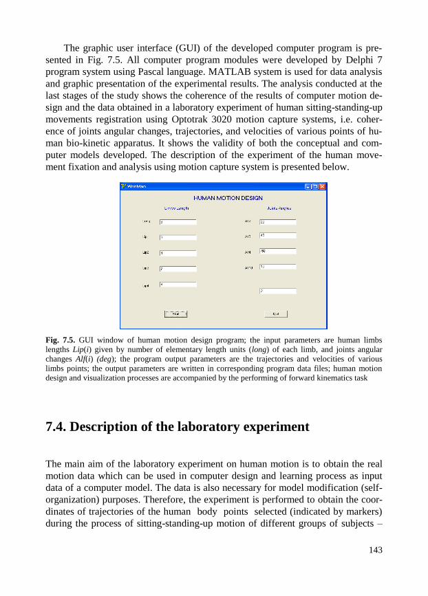
143
The graphic user interface (GUI) of the developed computer program is pre-
sented in Fig. 7.5. All computer program modules were developed by Delphi 7
program system using Pascal language. MATLAB system is used for data analysis
and graphic presentation of the experimental results. The analysis conducted at the
last stages of the study shows the coherence of the results of computer motion de-
sign and the data obtained in a laboratory experiment of human sitting-standing-up
movements registration using Optotrak 3020 motion capture systems, i.e. coher-
ence of joints angular changes, trajectories, and velocities of various points of hu-
man bio-kinetic apparatus. It shows the validity of both the conceptual and com-
puter models developed. The description of the experiment of the human move-
ment fixation and analysis using motion capture system is presented below.
Fig. 7.5. GUI window of human motion design program; the input parameters are human limbs
lengths Lip(i) given by number of elementary length units (long) of each limb, and joints angular
changes Alf(i) (deg); the program output parameters are the trajectories and velocities of various
limbs points; the output parameters are written in corresponding program data files; human motion
design and visualization processes are accompanied by the performing of forward kinematics task
7.4. Description of the laboratory experiment
The main aim of the laboratory experiment on human motion is to obtain the real
motion data which can be used in computer design and learning process as input
data of a computer model. The data is also necessary for model modification (self-
organization) purposes. Therefore, the experiment is performed to obtain the coor-
dinates of trajectories of the human body points selected (indicated by markers)
during the process of sitting-standing-up motion of different groups of subjects –

144
people of various height, mass, limb length, definition of relative joint angles
change, i.e. angular coefficients, which allow calculation of displacements, angular
velocities and accelerations, and comparison of the data obtained with the results
of computer human motion design.
Protocol of the laboratory experiment contains the following steps.
1. Choice of the criteria (characteristics are limb length, height, mass, number
of persons – subjects) for selecting an experimental group.
At this step the criteria for selecting groups of subjects being examined are
formulated. The following groups G1 and G2 of subjects were chosen according to
the predefined height criteria: 165-170 cm. for G1, and 175-180 cm. for G2. There
are 3 subjects in each group.
Fig. 7.6. Experiment scheme, where 1 is a subject – person being examined with markers placed
on his body, 2 is Optotrack camera, 3 is a computer, arrows are interconnections; measured values
are coordinates of markers; calculated ones: displacements, angles, velocities, accelerations
2. Definition of the standard sitting-standing-up posture.
The way of sitting-standing-up motion (way of legs, arms, and back positions
changing) performed by the subjects being examined was defined. All the experi-
ments were conducted with subjects standing in their initial position upright on the
floor with heels slightly apart (see Figs. 7.6-7.8) and parallel and elbows held close
to the torso. Their back was straight vertical. The arms were bent in the elbow
joints. Sitting-standing-up process was executed uniformly with little delay in low-
er down position. Heels were taken off the floor. Body was slightly bent forward.
2: Optotrack
3: Computer
1: Subject

145
3. Definition of the experiment conditions.
The following conditions of the experiment were defined: time of the sitting-
standing-up process (regulated during the registration process with the help of
a metronome) is 20 s.; the values being measured are coordinates (trajectories) of
markers placed on the predefined body points (Fig.7.9); scales of the measure-
ments: discrete moments on the time interval of 1/30 sec., scale of the measured
space is 3x3 m.; number of observations for each subject is 3.
4. Calibration of the Optotrack 3020 motion capture system.
Optotrack motion capture system was set according to the predefined experi-
ment scheme (see Figs. 7.6 and 7.7).
Fig. 7.7. One state of the laboratory experiment process: subject, i.e. person being examined, markers
placed on the shank, and camera of Optotrack motion capture system
5. Choice of the places of markers.
First, markers number 10, 11, and 12 were placed to define sagittal plane and
floor base surfaces (Fig. 7.8). After that, the other markers were placed in the defi-
nite points of human body to execute further measurements: two markers on foot,
and two on each limb, i.e. shank, thigh, leg, subject’s body side.
6. Execution of the measurements and data obtaining.
Data acquisition of markers coordinates is performed at each predefined mo-
ment of time. The markers trajectories are built after that. The data collected have
been given to MATLAB program system environment for further processing and
graphic presentation. Various markers coordinates in numeric format (Fig. 7.9) and
their trajectories in graphic format (Fig. 7.10) are plotted in MATLAB system.

146
Fig. 7.8. Places of markers and subject being examined
7. Measurement results processing.
The representative data is calculated using the dependence:
Xj(t)=ΣXj(t)i/n, (7.9)
where Xj(t) is X coordinate change of j marker, Xj(t)i is the X coordinate change of j
marker obtained in i observation, n is the number of observations.
8. Calculation of the joint rotation centers, limbs lengths as the distance be-
tween the joints rotation centers of correspondent limbs.
This procedure is executed by using the known mathematical relations. First,
the rotation centers are defined as the point of intersection of two lines each of
which is defined by two markers. After that, the limbs lengths are defined as a dis-
tance between the rotation points.
10
11
12
1
2
3
4
5
6
7
8

147
Fig. 7.9. Coordinates of various marker presented in the MATLAB table in numeric format
9. Calculations of correspondent displacements, angular velocities and angu-
lar coefficients for each group of subjects being examined.
To perform the calculations, special program functions were written in
MATLAB. One of the functions for joints angles calculation is presented in the
following form:
where i is the number of registrations of markers coordinates placed on the sub-
ject’s body; A(i, j) are fields of markers coordinates written in correspondent data
file while performing the laboratory experiment; fiSL is a correspondent ankle joint
angle between two limbs of human bio-kinetic apparatus – foot and leg in this case.
The results of relative angles calculation using the function presented above and
other functions are presented in Fig. 7.10.

148
Fig. 7.10. Human joints angular change – while performing sitting-standing-up motion – calculated
as a result of experimental data processing by program functions developed in MatLab system environment;
values of Fi angular change for each joint are given in degrees
10. Comparison of experimental and computer design data and prediction, i.e.
design, of other kinds of human sitting-standing-up motion.
The results of computer motion design and experimental data obtained by
Optotrack system for human sitting-standing-up motion were compared and ana-
lyzed. Prediction of motion is conducted for virtual subject with other limbs pa-
rameters. The results of prediction are compared with the data obtained from the
laboratory experiment with real subject with the same parameters (see Fig. 7.11).
Positive results of the analysis allows the validity to be stated of both conceptual
and computer models developed within the frameworks of the suggested HS design
method.
(deg)
Ankle joint angle
Foot toe joint angle
Knee joint angle
Femoral joint angle
(deg)
(deg) (deg)

149
a) b)
Fig. 7.11. Data analysis results: a) results of computer motion design for virtual subject with predefined
limbs parameters – program output data of exemplary ankle joint angular change of human bio-kinetic
apparatus, and b) data of ankle joint angular change obtained from laboratory experiment with real
subject with the same limb parameters – are given in both plots a) and b) after interpolation procedure;
values of Fi angular change are given in degrees
Preliminary conclusions and results
The main aim of the task described in this Chapter was HS conceptual model and
design method application in the design and control tasks of human motion. As a
result, a new HS method for human motion design was developed. The method
presents all the connected levels, i.e. human body structure (lower level), human
body dynamic representation as a unit in its environment, the environment struc-
ture (higher level), in common HS formal basis and takes into account geometric,
numeric, biomechanical and physical characteristics. The method developed allows
performing of the motion design task more sufficiently in comparison with tradi-
tional methods because of the functional abilities of the HS design method, such as
reconstructing the whole object being designed from its any structural element,
coordination of human movements and bio-kinetic apparatus deformations within
the frameworks of one common formal model, prediction of human motion, learn-
ing and others. The aim of the experimental study was to answer the question if the
computer design method developed corresponds to the real process of human mo-
tion, in our case to human sitting-standing-up movements, and if it is possible to
predict and coordinate (design and control) the human motion using the developed
program modules.
(deg) (deg)

150
To reach these aims, theoretical basis of the method suggested was described
in the work using hierarchical dynamic systems and aed coordination technology.
Coordination task of human motion was formulated, ways of motion design and
the method steps were defined, systems movements and deformations were de-
scribed within the frameworks of the suggested HS theoretical basis. Algorithm of
computer design and steps of the method realization for human sitting-standing-up
motion were given. Experimental study of human motion (using motion capture
system) and computer design with the motion prediction were performed. Compar-
ison of experimental and computer simulation results as well as the method analy-
sis were given.
The computer motion design was performed using a geometric model of hu-
man bio-kinetic apparatus constructed from conditional geometric objects (see
Chapter 4). The objects were presented according to HS aed model. The design
process of human sitting-standing-up motion was performed using initial experi-
mental data of one subject with definite parameters – limbs length and weights.
Prediction of motion was conducted for a virtual subject with other limbs parame-
ters. The results of computer prediction were compared with the data obtained in
the laboratory experiment with real subject with the same parameters. Coherence
of computer design and laboratory experiment results shows the efficiency of the
suggested HS design method. Exemplary analogous task of the traditional forward
kinematics task have been performed as the accompanying task within the frame-
works of the suggested method as a result of human sitting-standing-up motion
design and simulation.
As a result, new conceptual formal model and HS design method of human
motion coordination – design and control – have been created. The design method
has the following characteristics:
1) describes a human bio-kinetic apparatus as a hierarchical system; it allows
the design and control task of human motion to be performed as interconnections
coordination of coordinated structural and dynamic representation of man in its
environment;
2) makes possible designing (synthesis) of different kinds of human move-
ments, predicts the motion and obtains correspondent motion data using only the
geometrical or biomechanical data such as limbs length and weights; consecutive
interactive performing of the analysis design task, i.e. changing human structural
interactions (joint angles) and its subsystems characteristics – limbs length and
mass, and observation of the change of motion process being designed executed by
man in its environment (higher level system) allows obtaining the desired charac-
teristics of this process, i.e. trajectories coordinates, displacements, velocities, etc.;
3) connects three levels in common formal basis, such as the presentation of
human structure (bio-kinetic apparatus) and structural deformations (limbs motion
and joints angular change), description of human motion in environment (change

151
of human interactions with subsystems of environment), and construction of envi-
ronment (set of subsystems of higher level);
4) performs the connected tasks of human body deformations and human mo-
tion in its environment cased by these deformations within the frameworks of one
common HS aed model not using traditional approaches, i.e. Finite Elements
method and Integral Differential equations; allows performing of motion synthesis
and analysis tasks within the frameworks of one common computer model - soft-
ware construction.
5) allows presentation and processing of information of biomechatronic sub-
systems of various nature – mechanical, electronic, biomechanical, computer – in
frames of one common HS aed formal basis, what is very important in the case of
bio-mechanical, robotics, medical, rehabilitation and other systems coordination and
allows avoiding of modelling conflicts of various subsystems of different nature;
6) makes possible the modification of the developed conceptual and computer
models on the self-organization strata of coordinator, and motion prediction using
controlled experimental data;
7) presents the parts of human body in computer design as connected 3D ob-
jects due to the operations with HS models of conditional geometric objects (see
Chapter 4);
8) allows performing geometric design and forward kinematics tasks as a
common computational task owing to the description of geometric construction of
bio-kinetic apparatus, coordination (design and control) procedures and kinematic
characteristics within the frameworks of one common conceptual model.
Computer program created for human motions design has been constructed ac-
cording to HS structure, and the program functioning corresponds to the actions of aed
coordinator of HS. The design tasks are realized using commercial software Delphi
(Embarcadero Technologies Inc., CA, USA) and Matlab (The MathWorks Inc., MA,
USA) systems. All calculations effectively executed on computer as operations with
systems quantitative characteristics are presented in numeric positional code. During
the motion design, the dependences of functional parameters (kinds of motions) on
the structural ones (sizes, angles) of a human body segments were determined.
Creation of the HS theoretical basis, experimental study and computer simula-
tion of human motion are parts of the development process of aed conceptual mod-
el and HS method of human motion design. Theoretical constructions made possi-
ble the development of computer program modules which realize the technology of
the method. Experimental measurements obtained by the Optotrack motion capture
system and the results of simulation (computer experiment) of sitting-standing-up
human motion allowed the data comparison and the model validation. The results
of the conducted experimental study show the correspondence of the HS design
method and computer model developed to real processes of human motion and
wide abilities of HS design method in motion design.

152
8. DESIGN AND TESTING OF ELECTRONIC
CIRCUIT BOARDS
The conceptual model for design of an electronic Printed Circuit Boards (PCBs)
and HS technology of PCB quality testing is presented in this Chapter. The pro-
cesses of the PCB conceptual model creation and PCB quality testing take place at
the design and production phases of the general technological process of PCB life
cycle (see Fig. 1.2, Chapter 1). PCB conceptual design is realized in the industrial
PCB production process by human-computer CAD system coordinated by design
engineer. The quality of circuit boards is usually tested by a visual system – the
system of machine vision. To perform the PCB design and testing tasks, various
methods of PCBs synthesis and analysis are used nowadays for each particular case
[81-87].
The processes of synthesis and visual testing (analysis) of geometric construc-
tions of PCBs conductive pathways is described in this book using the proposed
conceptual design method using aed formal model and HS technology (see Chap-
ters 3 and 4). The task is also partially described in [88].
In the technological process of PCB production it is a usual situation for PCB
surface to have topological damages, such as conductive pathways breaks or joints.
So, the final stage of the technological process is the analysis of the PCBs quality.
Usually, the testing is realized as a video analysis, which contains the following
stages:
1) PCB graphic (standard) image creation,
2) obtaining a video-pattern of a tested PCB in one of graphic formats,
3) comparison of the obtained pattern with the standard image,
4) identification of PCB quality in the case of correspondence of a graphic
image of PCB to its standard and vice versa.
This approach, being based on standard methods of presentation and pro-
cessing of video-information (graphic images), has several drawbacks. The main of
them is the lack of coincidence between a graphic image of the board and the PCB
standard, which can occur during the third stage and is not caused by the quality of
a produced PCB. The reason is the changes of coordinates and the scale of the
153
graphic image of PCB obtained at the second stage, which is sometimes accidental-
ly caused by:
– the change of product’s (PCB) orientation in relation to the video camera;
– the change of the scale, i.e. distance between the video camera and the tested
PCB.
In each of these two cases the images of the standard and PCB being tested do
not coincides. As a result, a lot of PCBs of a good quality are recognized (at the
fourth stage) as defective goods.
The proposed conceptual design method is implemented in the form of a com-
puter program and allows the mentioned drawbacks to be avoided. It has the fol-
lowing steps:
1) geometric synthesis of standard of PCB – using HS conceptual design
method – with the formation of its graphic image (this stage is the part of the PCB
design phase as well),
2) obtaining a video-pattern – graphic image of the PCB being tested – in one
of graphic formats,
3) matching of the standard to the obtained image of PCB – coordination of
the PCBs orientation and scale,
4) comparison of the obtained image with PCB standard and pathways quality
testing,
5) PCB quality assessment.
Each of the above steps differs from the steps of a wide-spread technologies
of the task performing. For example, the task of geometric synthesis of the PCB
standard (1st step) is a part of the general PCB design task and corresponds to the
phase of geometric design of circuit boards.
Computer program realization of the PCB conceptual design method was used
in tasks of circuit boards design and testing at Horizont enterprise (Minsk, Bela-
rus). The scheme of the mechatronic unit – technological stand with machine vi-
sion system – for quality testing of conductive pathways of PCBs is presented in
Figure 8.1.
8.1. Geometric construction of circuit board
Geometric synthesis of the construction of PCB standard is the PCD design task
which is performed at both the conceptual design (CD) and detailed design (DD)
phases of the PCB life cycle (see Fig.1.2, Chapter 1). At the same time, it (geomet-
ric synthesis of PCB standard) is the first stage of the HS design method realiza-

154
tion for visual analysis – quality testing – of conductive pathways of electronic
printed circuit boards (PCBs).
Fig. 8.1. Technological stand with mashine vision unit for PCB quality testing: 1 – personal computer;
2 – video camera control board; 3 – controller of coordinates; 4 – video camera; 5 – drive of coordinate X;
6 – drive of coordinate Y; 7 – drive of coordinate Z; 8 – circuit board being tested
Geometric construction of conductive pathways of PCBs is presented in ac-
cordance with (4.1) in the following (8.1) form:
},,{ 0 SS gg , (8.1)
where: – aggregated description of the construction as a unit in its environment,
– structure of interconnections,
0S – coordinator, which connects and , and therefore the higher and
lower levels of the PCB construction,
g – index, which shows the geometrical nature of the mechatronic system un-
der consideration.
Structure is defined according to (4.3) as follows:
}},{,{ 10
S , (8.2)
1

155
and contains aggregated representations 1 of PCB geometric elements of the
lower level, their interconnections and coordinator
0S which sets relations
between the elements.
Coordinator is presented according to (3.15) in the following (8.3) form:
000 },,{ SS , (8.3)
and in this case is implemented by a computer program as a law of interlevel con-
nections and as rules in accordance with which the geometric elements were con-
nected in geometric constructions of PCBs on different levels.
Quantitative and metrical characteristics of elements 1 , i.e. conductive
pathways, and the addresses of their connections are defined in codes of the
numeric positional system (4.9-4.14).
Geometric construction of PCB conductive pathways is created by 0S using
one of its coordination strategies (see Chapters 3 and 4). According to (4.4), coor-
dinator synthesizes the structure of pathways from subsystems 1 of three lev-
els:
},{: 10S , (8.4)
where = -2, -1, .
On level -2 the parts of conductive pathways are constructed from condi-
tional points 3 presented in the form of quadrates (Fig. 8.2). Number n and
sizes w01 of -3 level elements define width w1
1 and length 12 =l=wn of
-2 level segment of pathway.
i=1 i=n
2 :
w l=wn 3
Fig. 8.2. Structure 2 of a pathway segment constructed from conditional points
3
This process is described at conceptual design (CD) phase as follows:
= -2, . (8.5) 22320 },{: S
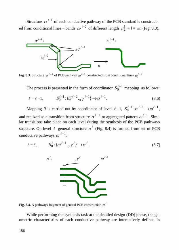
156
Structure of each conductive pathway of the PCB standard is construct-
ed from conditional lines – bands of different length = l = wn (Fig. 8.3).
1 : 1 :
Fig. 8.3. Structure 1 of PCB pathway 1 constructed from conditional lines 2i
The process is presented in the form of coordinator 1
0S mapping as follows:
= –1, 1121
0 },{: S . (8.6)
Mapping R is carried out by coordinator of level –1, 111
0 : S ,
and realized as a transition from structure 1 to aggregated pattern
1 . Simi-
lar transitions take place on each level during the synthesis of the PCB pathways
structure. On level general structure (Fig. 8.4) is formed from set of PCB
conductive pathways 1 :
= , },{: 1
0S . (8.7)
: 1
Fig. 8.4. A pathways fragment of general PCB construction
While performing the synthesis task at the detailed design (DD) phase, the ge-
ometric characteristics of each conductive pathway are interactively defined in
12 1
2
R
1
2i
157
program realization and written in typical computer files. The pathways are also
defined as a set of parameters which are presented in typical files in the form of
corresponding numeric codes. While any of the pathway elements is changed, the
others are automatically reconstructed by coordinator – presented in the form of
computer control program – with simultaneous change of corresponding pro-
gram codes. That is possible thanks to the availability of the connections between
the pathways elements – conditional geometric objects (see Figs. 8.2 and 8.3). It
allows easy correction of the geometric structure of PCB conductive pathways at
any stage of its synthesis and reconstruction processes.
The availability of mechanism of information aggregation
allows
the reduction of computer memory volumes in the process of transition to a higher
level of the PCB geometric structure during its formation. The basic result in com-
parison with well known PCB design and testing approaches is that the graphic
image of PCB is obtained in the process of construction of PCB geometric repre-
sentation. The availability of transition from the graphic image to geometric repre-
sentation and vice versa allows effective adaptation of the PCB geometric structure
at testing stages 2-5, in particular at the stage of adaptation of the standard to the
received graphic image, when coordinates and scales are in process of changing.
8.2. Stages of PCB interconnections quality testing
Structure of information in the process of PCB testing is also presented in aed form
(3.1). But in this case we have a system for which the construction of geometric
representation Sg (stage 1) is structural element
, and is the graphic image
of interconnections. PCB image is presented as follows:
},,{ vs , (8.8)
where: s is graphic representation of standard; v is received video-image of
PCB, – connections of and (for instance, three points of the images,
by which the coordination of images is determined).
PCB testing process corresponds to 2-5 stages described above, which are ex-
ecuted in a technological process of PCB production. In comparison with the
known approaches, stage 2 of the proposed method is almost the same as for
known technologies and realized by using standard video cameras, e.g. Chameleon
s v

158
[89] or Grasshopper [90] cameras. The exemplary PCB image obtained while task
performing is presented in Fig. 8.5.
Fig. 8.5. The result of obtaining a PCB video image
a) b)
Fig. 8.6. The results of the PCB image processing: a) imcrop function application, b) the result
of rgb2gray and edge functions application
The obtained PCB image is preprocessed to be fit for the next steps of the PCB
quality testing. The results of the image processing – the fragment acquisition and
edges extracting of conductive pathways are presented in Fig. 8.6 a), and Fig. 8.6
b) accordingly.
For the PCB fragment acquisition the Matlab imcrop function is used. To ex-
tract the edges of the conductive pathways the edge function of the Matlab Image
Processing Toolbox is applied.
The matching process of the PCB standard (stage 3) is usually not presented in
widespread testing technologies. At this stage in frames of the proposed method,

159
the PCB standard is built on to PCB image by its three basic points, which allow to
coordinate the orientation and sizes of the standard and the received graphic image
of PCB thanks to the availability of its HS geometric representation.
a) b)
c) d)
Fig. 8.7. Images a)-c) of PCB conductive pathways of different orientation and scales obtained
from computer monitor; d) is the image of the pathways presented in grey format
It permits to avoid disparity between the standard and the image which is
caused not by damages of PCB but by changes of PCB scale, i.e. camera distance
from it, and orientation (Fig. 8.7). The matching process of graphic images is real-
ized after definition of matching control points using Matlab functions of Image
Processing Toolbox and Computer Vision System Toolbox [91]. The results of the
matching process of the obtained PCB fragment and PCB standard images is pre-
sented in Fig. 8.8.

160
Fig. 8.8. Matching of PCB fragment images of different orientation and scale, axes units are pixels
Standard Matlab procedures allow realization of images fitting by using of im-
rotate() and imresize() functions, detecting features applying in both images to be
matched detectSURFFeatures() function, and extract feature descriptors using ex-
tractFeatures() function. Matching features by using their descriptors is realized
with help of matchFeatures() function. This function also allows computing the
transformation from the obtained PCB fragment image to the original PCB stand-
ard image. The matching process of the two PCB images, i.e. original (o) image –
red, and distorted one (+) – blue, is presented in Fig. 8.8.
PCB image obtaining is performed using standard digital cameras to match the
image of PCB standard. Exemplary fragment of pathways structure of PCB stand-
ard (Fig. 8.7) was synthesized using Pascal programming language. The images of
PCB conductive pathways of different orientation and scales presented in Fig. 8.7
are the screenshots obtained from a computer monitor.
At the fourth stage of PCB quality testing, comparison and detection of PCB
defects is carried out with regard to the geometric representation of PCB standard
by checking the conductive pathways for the gaps (Fig. 8.9a) – not by continuous
scanning of image lines, as in usual technologies, but by scanning along the con-
ductive pathways structures. It allows the time of comparison process and volumes
of processed information to be reduced.
In the process of pathways soldered joints test, the aperture moves along the
imaginary construction (Fig. 8.9b) which corresponds to the construction of i inter-
connection (і, і+1 – the neighbouring pathways).

161
a) test of gaps b) test of joints
Fig. 8.9. Schemes of a) gaps and b) soldered joints testing processes
The fifth stage of the PCB quality assessment is a simple logic operation over
the results of the fourth stage.
Preliminary conclusions and results
The introduced PCB conceptual design method and HS technology of PCBs con-
ductive pathways quality testing yields the following main results:
– a graphic image of PCB standard is a result of formation of geometric repre-
sentation of PCB in the process of synthesis of PCB pathways construction;
– availability of geometric representation allows easy correction of pathways
topology at each phase of PCB constructing, including conceptual design (CD) and
detailed design (DD) phases;
– the mechanism of information aggregation permits to avoid the growth of
computer memory volumes during the growth of the PCB construction level in the
design and production processes;
– the PCB testing technology gained new qualities: the possibility of scales
and orientation of PCB pathways geometric construction to change (during PCB
standard rebuilding on to the obtained graphic image of PCB) allows to avoid the
identification of PCB quality as defective in a technological process, when the
PCB orientation and the distance in relation to the video camera are changed;
– the standard and obtained PCB images are compared not by continuous
scanning of image lines as in usual technologies, but only by scanning along the
conductive pathways with regard to the pathways geometric representation, which
allows the reduction of the time of comparison and computer memory volumes.
i+1
joint
gap
window
window i

162
9. DESIGN AND CONTROL
OF MCM CUTTING MACHINE
In this Chapter, the conceptual model, design (synthesis and analysis) and motion
planning tasks of MCM machine are described. MCM – Manhole Cutting Machine
– is used in production environment to perform technological operations of pipes cut-
ting and welding [92-94]. At the Conceptual Design (CD) phase of MCM life cycle,
the systemic formal models of MCM elements and coordination (design and con-
trol) processes were presented in HS theoretical basis (see Chapters 3,4). At the
Detailed Design (DD) phase, much attention is paid to the MCM analysis – kinemat-
ics tasks, and synthesis – the task of MCM construction creation. Different concrete
elements which potentially could be used in MCM structure were analyzed to per-
form the synthesis task. Construction and technologies of the control subsystems, i.e.
Mobile Panel of 5MP050.0653-03 type, ARNCO soft CNC system, Automation
Studio program environment [95], as well as actuators, e.g. ACOPOS servo drivers
of B&R [96] were analyzed. Systemic formal models of these systems were also
given at the CD phase before realizing synthesis task at the DD phase.
According to the definition of the conceptual model given in Chapters 3 and 4,
the developed conceptual model of MCM machine presented below contains for-
mal descriptions of MCM structure and its environment, dynamic models of struc-
tural elements and their connections, functional model of MCM machine and its
coordinator. The coordinator is presented as a system which realizes the design and
control processes and connects in this way structure and functions of MCM ma-
chine. The suggested conceptual model of MCM machine is also partially de-
scribed in [94].

163
9.1. MCM conceptual model
Conceptual model of MCM machine (Manhole Cutting Machine) is given in the
formal basis of HS using its standard block aed (3.1), see Chapter 3, and is pre-
sented as follows:
S { , 0S ,
}, (9.1)
where is functional dynamic description of MCM machine in its technological
environment S ,
is MCM structure, 0S is coordinator, is index of level,
Ls, Ls is numeric positional system. According to aed scheme (see Fig. 3.1),
formal description S contains the object (MCM) model
So and models of
MCM sub-systems io S , production environment
S model, models of coordina-
tor 0S (design and control system of MCM) and technological process
S per-
formed by MCM, i.e. cutting and welding.
Functional descriptions of MCM system So is presented according to (3.2)
in the following form of dynamic system , :
TtYXC ttttooo &::, , (9.2)
ttTttCXC ttttttoo &,&: ,
whre T is time of level;
C , X ,
Y are state, input and output of MCM So
system respectively; is state transition function, is the reaction.
Structure of MCM is defined according to (3.13) as the following formal
system:
{0S ,{
1 , }} {
0S , ~ }, (9.3)
where 0S is coordinator of MCM,
1 are dynamic models ( , ) of MCM
subsystems }:{ 11 IiSS i ,
are structural connections.
Structure of MCM is created while performing synthesis task at both CD and
DD phases. In our case, structure of MCM was created within the frames of
SolidWorks system environment [74], see Fig. 9.1. After that, MCM model was
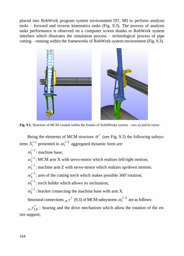
164
placed into RobWork program system environment [97, 98] to perform analysis
tasks – forward and inverse kinematics tasks (Fig. 9.3). The process of analysis
tasks performance is observed on a computer screen thanks to RobWork system
interface which illustrates the simulation process – technological process of pipe
cutting – running within the frameworks of RobWork system environment (Fig. 9.3).
Fig. 9.1. Structure of MCM created within the frames of SolidWorks system – two a) and b) views
Being the elements of MCM structure (see Fig. 9.2) the following subsys-
tems 1
iS presented in 1
i aggregated dynamic form are:
11 : machine base;
12 : MCM arm X with servo-motor which realizes left/right motion;
13 : machine arm Z with servo-motor which realizes up/down motion;
14 : arm of the cutting torch which makes possible 360o rotation;
15 : torch holder which allows its inclination;
16 : bracket connecting the machine base with arm X.
Structural connections (9.3) of MCM subsystems
1i are as follows:
:6,1 bearing and the drive mechanism which allow the rotation of the en-
tire support;

165
:2,1 rack begin the connection which allows the displacement of X arm
relative to MCM base;
rack begin the connection which allows the displacement of Z arm
relative to X arm;
bearing which makes possible 360o rotation of torch arm;
bevel gear used for the cutting torch inclination.
Fig. 9.2. Axis and structure of MCM machine
Fig. 9.3. MCM design model placed into RobWork simulation system environment to perform analysis
– forward and inverse kinematics – tasks while simulating technological process of pipe cutting;
the MCM environment elements – pipe (grey color) with hole being cut and support (red color) –
are elements of the technological module
:3,2
:4,3
:5,4

166
Environment of MCM machine contains the other technological units and
a man-operator. Elements of environment structure which are in direct
contact with MCM machine are a pipe being cut and support . The
support allows the piper rotation in the technological cutting process (see Fig. 9.3).
Pipe being cut is colored grey in Figure 9.3 and the support is colored red.
Fig. 9.4. General process So and sub-processes
io S performed by MCM;
1S and
2
S
are sub-processes executed in MCM environment
S
S
1
So2So
1
So2So
1
S : measurement of frames
by cross-system
2
S : machining of a part
with a predefined parameters
2
So : shape generation based on the introduced samples
5So : selection of base point and G-code generation
3So : introduction of velocity and offset parameters
4So : recipe saving to CF card file
6So : choice of MCM function: cutting, welding or chamfering
So
1
So : introduction of samples to machine’s memory

167
General process and sub-processes which are executed by MCM
while performing pipe cutting operations are presented in Figure 9.4. Each of the
sub-processes is described by dynamic model at CD phase. The
descriptions are concretized at DD phase.
Within the frameworks of the suggested MCM conceptual model the coordina-
tor is presented in the form of the design and control system of MCM machine.
MCM coordinator is formally described by (3.15) equation. performs the
design and control tasks on its selection, learning and self-organization strata.
Dynamic realizations of coordinator strata are presented by canonic models
0 ↔{
0)ˆ,ˆ( ,
0S } (see Chapter 3) in the following form:
}'&',&:ˆ{ˆ0'00'00 ttTttCXC tttt , (9.4)
}&~~
:ˆ{ˆ00000
TtYXCtt .
Canonic model [94] is constructed using the concept of the multilayer (multi-
strata) system, where states transition functions {0 } correspond to learning and
self-organization strata, and output functions {0 } correspond to the strategies of
the selection strata.
The developed block-scheme of elements 20S ,2
10S of coordinator
0S being the
control system of servomotor S2 of MCM arm is presented in Figure 9.5, where:
G is control signal u_set[v]=e(t) which is realized with the help of B&R
technology [96] and goes from ACOPOS controller 20S to servomotor
S2 ;
W is the feedback from controller 20S , realized in the form of impulses
s_act[inc];
1G is the control signal from PC panel 21
0S to controller 2
0S presented in
the format {position (s), velocity (v), acceleration (d2s/ dt2), delay (- d2s/ dt2)}; 1W feedback to PC panel
10S presented in the format {status (ena-
ble/disable), position (s), velocity (v), error (error)}; 2X is the servomotor input – electromotive force E(t) (Fig.9.5);
2Y is the servomotor output – torque )(tm .
Soio S
io S
),(
0S
0S

168
Canonic model of the controller 2 in the form of (9.4) is built using objects
of inputs ={ , }, outputs ={ , } and states of coordinator
2 , where is state of Acopos 2 controller.
Fig. 9.5. Conceptual scheme of control system of MCM arm servomotor presented in coordinator
form
Canonic model of the controller 2 in the form of (9.4) is built using objects
of inputs ={ , }, outputs ={ , } and states of coordinator
2 , where is state of Acopos 2 controller.
At the detailed design phase, control system is created by the selection of con-
crete elements and realization of their structural connections. In this way the syn-
thesis design task is performed. Formal description of this task (9.8) is given be-
low. Concrete system based on ACOPOS servo-motors control and synthesized at
DD phase for MCM arms motion control is presented in Figure 9.6. Here the ele-
ments, i.e. ACOPOS servo drives, X67 input-output units, X20 control and remote
I/O systems, visualization and operation system, are connected by the network
using CAN bus.
The following stuctural elements are presented In Figure 9.6. ACOPOS 1045
is an intelligent servodrive [99] with very short scan times and communication
cycles of 400 µs, which equal to 50 µs in the control loop. Intelligent ACOPOS
0S
0X 1G W
0Y G 1W
0C
0S
0C 0S
0S
0X 1G W
0Y G 1W
0C
0S
0C 0S
2Y
2X
0S
G W
02 S
ACOPOS controller
S2 servomotor
1G 1W
S
1
02
S
PC Power Panel
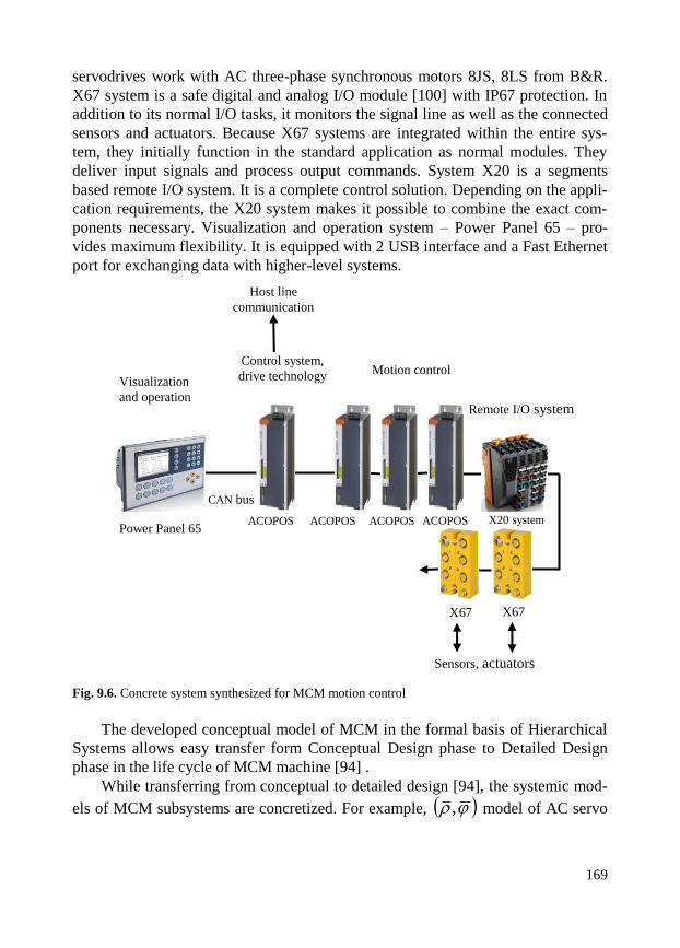
169
servodrives work with AC three-phase synchronous motors 8JS, 8LS from B&R.
X67 system is a safe digital and analog I/O module [100] with IP67 protection. In
addition to its normal I/O tasks, it monitors the signal line as well as the connected
sensors and actuators. Because X67 systems are integrated within the entire sys-
tem, they initially function in the standard application as normal modules. They
deliver input signals and process output commands. System X20 is a segments
based remote I/O system. It is a complete control solution. Depending on the appli-
cation requirements, the X20 system makes it possible to combine the exact com-
ponents necessary. Visualization and operation system – Power Panel 65 – pro-
vides maximum flexibility. It is equipped with 2 USB interface and a Fast Ethernet
port for exchanging data with higher-level systems.
Fig. 9.6. Concrete system synthesized for MCM motion control
The developed conceptual model of MCM in the formal basis of Hierarchical
Systems allows easy transfer form Conceptual Design phase to Detailed Design
phase in the life cycle of MCM machine [94] .
While transferring from conceptual to detailed design [94], the systemic mod-
els of MCM subsystems are concretized. For example, , model of AC servo
Host line
communication
Power Panel 65 ACOPOS
CAN bus
Control system,
drive technology
X20 system
Remote I/O system
ACOPOS ACOPOS ACOPOS
Visualization
and operation
X67 X67
Motion control
Sensors, actuators

170
motor S2 (Fig. 9.7) being the element of the machine arm is presented in the
following form (9.5) of DE:
uayadt
dya 210 (9.5)
which is concretized and presented at the DD phase as follows [101]:
))2(32(3
1 '''cbamasbcab
sa piRvv
Li
dt
d
))2(3(3
1 '''cbambsbcab
sb piRvv
Li
dt
d
)( bab idt
di
dt
di
dt
d (9.6)
)( '''ccbbaae iiipT
)(1
mmfem TFTTJdt
d
mdt
d
where equations (9.6) correspond to the states transition functions of the con-
ceptual model ( , ), (see Fig. 9.8). DEs (9.6) are further transformed at the DD
phase to the transfer function (9.7):
)(
)()(
sT
ssG
em
m (9.7)
a) b)
Fig. 9.7. CAD model of AC 8BJ motor of B&R (a) [99], and its Matlab simulation scheme (b) [101]

171
In Figure 9.8 and equations (9.6) and (9.7), the variables are as follows: Ls is
the inductance of the stator; Rs is a resistance of the stator; ia, ib, ic are currents of
a, b and c phases respectively; Φa', Φb
', Φc' are electromotive forces of a, b and c
phases respectively; vab, vbc are ab and bc phase to phase voltages respectively; ωm
is angular velocity of the rotor; λ is the amplitude of the flux induced by the per-
manent magnets of the rotor in the stator phases; p is number of pole pairs; Tem
is electromagnetic torque; J is combined inertia of rotor and load; F is combined
viscous friction of rotor and load; θ is rotor angular position; Tm is shaft mechani-
cal torque; Tf is shaft static friction torque; ωm is angular velocity of the rotor –
mechanical speed.
Fig. 9.8. Steps of conceptual model , concretization of AC servo-motor subsystem 2
i
at the design phases of MCM life cycle; conceptual model is transformed to ordinary DE and concretized
at DD phase by transfer function G(s)
9.2. Design tasks
The main design tasks – synthesis & analysis – are performed at both conceptual
and detailed design phases. The first basic design task which is performed by
MCM coordinator is the synthesis task. In the basis of the conceptual model de-
scribed above and the general formulation of the synthesis task within the frame-
works of HS technology, the structure of the MCM machine being synthesized is
presented in form (9.8), and the synthesis operations are described by ),( mod-
els of coordinator processes 0S . In the process of performing a synthesis task in
SolidWorks system environment the robot structure σl is synthesized from its ele-
ments ωl-1 by realizing structural connections σγl. The task is described at CD phase
within the frameworks of HS conceptual model as coordinator 0S task as follows:
},{: 10S . (9.8)
I
Conceptual
model
),(
DETAILED DESIGN phase 3
II
III CONCEPTUAL DESIGN phase 2
Ordinary DE
uayadt
dya 210
Concrete DE
)( '''ccbbaae iiipT
)(1
mmfem TFTTJdt
d
Transfer
function
)(
)()(
sT
ssG
e
m
IV

172
Geometric parameters of the MCM structure itself are changeable in the syn-
thesis process. At CD phase the parameters are described by constructive dimen-
sion and connections defect, introduced in Section 4.2 by numerical positional
system. At DD phase the concrete sizes as well as physical characteristics of
MCM parts are defined.
In the synthesis process, MCM structure dynamics is described by reaction ρ
of (ρ,φ) model:
}&:{ TtYXC tttt (9.9)
where: Ci is the initial MCM part at t=i moment of time (or composition of previ-
ously connected parts in the synthesis process), Xi is a part to be added, Yi is the
union (composition) of Ci and Xi parts, t=i – moment of time T. The exemplary
MCM machine construction synthesized within the frameworks of SolidWorks
system and placed in RobWork system environment is presented in Figs. 9.3 and
9.11.
At the detailed design (DD) phase the concrete MCM machine parts were cho-
sen, e.g. the ACOPOS servo drivers of B&R [99], Mobile Panel of 5MP050.0653-
03 type, ARNCO soft CNC system, Automation Studio program system [95], etc.
Parts of the MCM mechanical arm were produced in Promotech enterprise (Bi-
alystok, Poland). MCM arm parameters were defined after stress and materials
analysis performing. The results of the synthesis for the cases of MCM mechanical
construction and MCM arms motors control system are given in Figs. 9.2-9.3, and
Fig. 9.6 respectively.
Fig. 9.9. Steps of conceptual model concretization at the design phases of MCM life cycle; conceptual
model is transformed to object’s reaction to and concretized at DD phase by kinematics equations
The analysis design tasks are kinematics and dynamics tasks. To perform the
kinematics task, kinematic scheme of MCM is developed (see Fig. 9.10c ) at the
CD phase, kinematic model of MCM is presented in ),( form and transformed
to the form of reaction to model. At the DD phase, a mathematical model of
I
Conceptual
model
),(
DETAILED DESIGN phase 3
II III
CONCEPTUAL DESIGN phase 2
Object’s reaction
TtYXC tttto &:
Forward kinematics equations
arlxxg sinsin0
xarlyyg sincos0
zalzzg cos0

173
MCM kinematics is created as concretization of the conceptual model and present-
ed in the form of forward kinematics equations [46,93], see Figure 9.9.
The scheme presented in Figure 9.9 shows the dynamics of the object’s kine-
matic model – MCM machine – in its design process. Transformation of the model
of MCM dynamics is realized in the similar way. The construction and kinematic
scheme of the MCM machine are given in Figure 9.10, where the pipe being cut,
MCM axis and both global “G,O” and detail “D” coordinate systems are presented
as well.
The aim of the kinematics task performed at the DD phase is the definition of
the locations and orientations of MCM tool – operating point of the cutting torch.
The equations created at DD phase (Fig. 9.9) which define the MCM end effecter
(TCP – tool center point) position in global “G,O” coordinates are as follows:
arlxxg sinsin0
xarlyyg sincos0 (9.10)
zalzzg cos0 ,
where
0 0,03068x
0 2,40975y (9.11)
0 1,45775z
0,113 offsetl ,
x0, y0, z0 are parameters connected with the machine geometry (m); l is the ef-
fective tool length (m); x, z, r, a, d are the locations of each machine axis (m).
Position of the end effecter in detail coordinate system „D” is described by the
following equations:
dzdxx ggd sincos
dzdxy ggd cossin (9.12)
gd yz
where xd, yd, zd are coordinates of the end effecter (TCP) in the detail coordinate
system „D”; xg, yg, zg are coordinates of the end effecter in the global coordinate
system „ O”.
To perform the forward kinematics task the following algorithm was developed [93].

174
a) b)
c) d)
Fig. 9.10. Coordinate systems a) and d) – d) is a computer screen-short, MCM axis b) and d),
and kinematic scheme c) of MCM, where D is the coordinates system connected with the pipe detail,
O is the global coordinates system, R is the reference frame of the instrument holder rotation joint,
A is the reference frame of the tool rotation joint
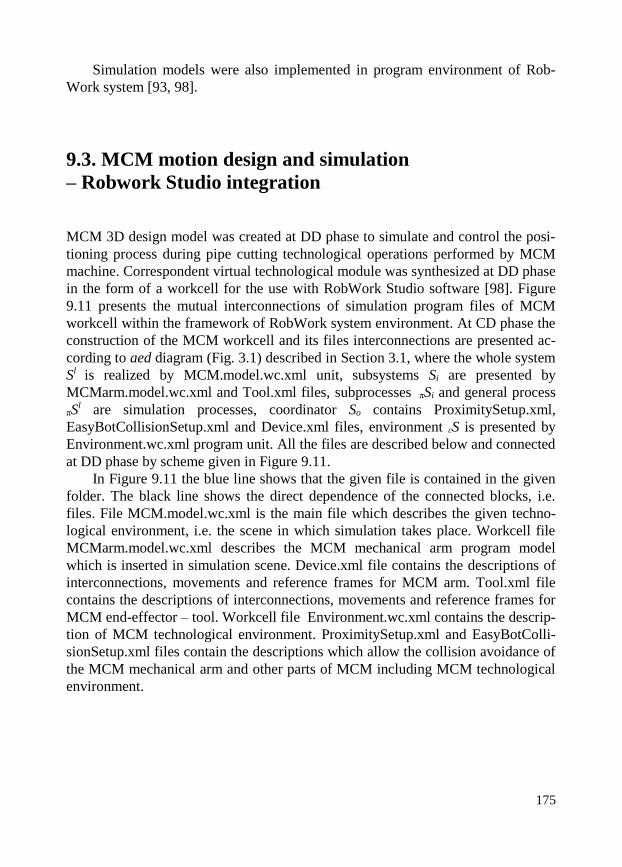
175
Simulation models were also implemented in program environment of Rob-
Work system [93, 98].
9.3. MCM motion design and simulation
– Robwork Studio integration
MCM 3D design model was created at DD phase to simulate and control the posi-
tioning process during pipe cutting technological operations performed by MCM
machine. Correspondent virtual technological module was synthesized at DD phase
in the form of a workcell for the use with RobWork Studio software [98]. Figure
9.11 presents the mutual interconnections of simulation program files of MCM
workcell within the framework of RobWork system environment. At CD phase the
construction of the MCM workcell and its files interconnections are presented ac-
cording to aed diagram (Fig. 3.1) described in Section 3.1, where the whole system
Sl is realized by MCM.model.wc.xml unit, subsystems Si are presented by
MCMarm.model.wc.xml and Tool.xml files, subprocesses πSi and general process
πSl are simulation processes, coordinator So contains ProximitySetup.xml,
EasyBotCollisionSetup.xml and Device.xml files, environment εS is presented by
Environment.wc.xml program unit. All the files are described below and connected
at DD phase by scheme given in Figure 9.11.
In Figure 9.11 the blue line shows that the given file is contained in the given
folder. The black line shows the direct dependence of the connected blocks, i.e.
files. File MCM.model.wc.xml is the main file which describes the given techno-
logical environment, i.e. the scene in which simulation takes place. Workcell file
MCMarm.model.wc.xml describes the MCM mechanical arm program model
which is inserted in simulation scene. Device.xml file contains the descriptions of
interconnections, movements and reference frames for MCM arm. Tool.xml file
contains the descriptions of interconnections, movements and reference frames for
MCM end-effector – tool. Workcell file Environment.wc.xml contains the descrip-
tion of MCM technological environment. ProximitySetup.xml and EasyBotColli-
sionSetup.xml files contain the descriptions which allow the collision avoidance of
the MCM mechanical arm and other parts of MCM including MCM technological
environment.

176
/Scene/ /geometry/ /MCM/ /MCMtool/
/MCM/geometry/ Tool/geometry/
Fig. 9.11. Interconnections of simulation program files of MCM workcell in RobWork system
Fig. 9.12. Two states of hole cutting process simulated in RobWork system environment and meanings
of correspondent parameters
MCM.model.wc.xml
„files.stl”
MCM stand elements
ProximitySetup.xml
Environment.wc.xml MCMarm.model.wc.xml
Device.xml
„files.stl”
End effector parts
ProximitySetup.xml
EasyBotCollisionSetup.xml
Tool.xml
„files.stl”
MCM arm parts
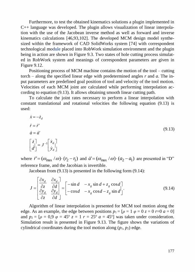
177
Furthermore, to test the obtained kinematics solutions a plugin implemented in
C++ language was developed. The plugin allows visualization of linear interpola-
tion with the use of the Jacobean inverse method as well as forward and inverse
kinematics calculations [46,93,102]. The developed MCM design model synthe-
sized within the framework of CAD SolidWorks system [74] with correspondent
technological module placed into RobWork simulation environment and the plugin
being in action are shown in Figure 9.3. Two states of hole cutting process simulat-
ed in RobWork system and meanings of correspondent parameters are given in
Figure 9.12.
Positioning process of MCM machine contains the motion of the tool – cutting
torch – along the specified linear edge with predetermined angles r and a. The in-
put parameters are predefined goal position of tool and velocity of the tool motion.
Velocities of each MCM joint are calculated while performing interpolation ac-
cording to equation (9.13). It allows obtaining smooth linear cutting path.
To calculate the joint rates necessary to perform a linear interpolation with
constant translational and rotational velocities the following equation (9.13) is
used:
dzx
'
'
aa
rr
(9.13)
d
d
y
xJ
d
z
1
where )()/(' 12max rrr and )()/(' 12max aaa are presented in “D”
reference frame, and the Jacobian is invertible.
Jacobean from (9.13) is presented in the following form (9.14):
dzdxd
dzdxd
d
y
z
yd
x
z
x
Jgg
gg
dd
dd
sincoscos
cossinsin. (9.14)
Algorithm of linear interpolation is presented for MCM tool motion along the
edge. As an example, the edge between positions p1 = [ρ = 1 φ = 0 z = 0 r=0 a = 0]
and p2 = [ρ = 0,9 φ = 45o z = 1 r = 25o a = 45o] was taken under consideration.
Simulation result is presented in Figure 9.13. The figure shows the variations of
cylindrical coordinates during the tool motion along (p1, p2) edge.
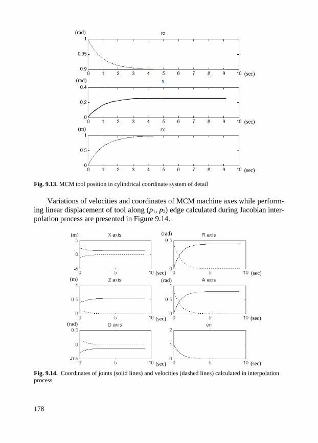
178
Fig. 9.13. MCM tool position in cylindrical coordinate system of detail
Variations of velocities and coordinates of MCM machine axes while perform-
ing linear displacement of tool along (p1, p2) edge calculated during Jacobian inter-
polation process are presented in Figure 9.14.
Fig. 9.14. Coordinates of joints (solid lines) and velocities (dashed lines) calculated in interpolation
process
(m)
(m)
(rad)
(rad) (sec)
(sec)
(sec)
(sec)
(rad)
(sec)
(sec)
(rad)
(rad)
(m)
(sec)
(sec)
(sec)
(
s
e
c
)

179
In our case, due to the presented MCM machine design, i.e. the choice of
joints axes, the joint velocities calculation is simplified in a marked degree. Tool
orientation is directly correlated to axes motions, and also the motion along z axis
in ‘D’ coordinate system is governed by the x axis translation. According to these
considerations, it is only necessary to calculate Jacobian relating (xd, yd) coordi-
nates to z and d joint positions.
Preliminary conclusions
The use of Hierarchical Systems (HS) method in design and control of MCM
(Manhole Cutting Machine) is presented in this Chapter. Being mechatronic by
nature, MCM system contains human – man-operator, computer control, visual
informatics, electronic – sensors, electromechanical – servo drives, and executive
mechanical (MCM tool, arm and its joints) subsystems. The presented conceptual
model of the MCM system being designed contains connected systemic models of
the above mentioned subsystems presented in the general formal basis. Aed (stand-
ard block of HS) model, see Chapter 3, was chosen as the formal basis of MCM
conceptual model. The MCM system structure, its dynamic presentation as the unit
in its technological environment, MCM environment – other objects and techno-
logical units of the production process, and MCM control unit – ACOPOS control-
ler – were also described in this basis. MCM design and control functions are taken
into account owing to HS coordinator availability. Coordinator performs coordina-
tion (design and control) tasks on its selection, learning and self-organization strata.
The presented conceptual formal model of MCM machine is coordinated with
traditional systems of information presentation in mechatronics [103-112]: numeri-
cal, graphic and natural language forms [8, 127]. Being the formal basis of MCM
conceptual model, aed technology and HS method are coordinated with general
requirements of design and control systems and allow easy transfer from Concep-
tual Design to Detailed Design phase in MCM life cycle. It brings new possibilities
to creating a formal language for MCM and similar technological machines con-
ceptual design. The process of MCM conceptual model creation as well as MCM
design and control processes were executed within the framework of the R&D
project maintained by the agreements RO-210.0610/25/2013 – U/WM/7/2013 and
U/WM/7/2014 – between Bialystok University of Technology and Promotech en-
terprise (Bialystok, Poland).

180
CONCLUSION
The new hierarchical systems (HS) method – theoretical and practical computer
means – of conceptual design of mechatronic systems based on HS theory and
oriented towards usage in automation systems including CAD, automatic control,
robotics and mechatronics is described in the given book. The presented process of
the method development contains the following phases.
First, the theoretical basis for the design method, i.e. aed theoretical construc-
tion of HS and formal model of its coordinator, was constructed.
Second, after creating the mathematical model, the HS coordinator was pre-
sented in this book in the form of theoretical construction of aed-processor – the
cybernetic system oriented to numerical and geometric information presentation
and processing while performing design tasks. It was shown that the processor is
able to execute operations with real, natural, complex and hyper-complex numbers
in the frames of one common formal construction. This processor is oriented to-
wards the geometric information processing presented in numerical code.
The theoretical construction of the core element of design systems, i.e. aed
model created, and its coordinator symbol construction have the following charac-
teristic features:
aed includes the dynamic structure and aggregated models of any system be-
ing coordinated – designed and controlled – and its environment, and allows the
main design task to be carried out with the help of coordination strategies for the
different levels of knowledge uncertainty;
coordination strategies are the states of a design and control system, their dy-
namics (like the process of uncertainty removal) reflects the dynamics of that sys-
tem;
the ability of aed for self-organization (with the following alteration of any de-
signed system model and coordination strategies) is ensured thanks to the availabil-
ity of higher strata of the coordinator;
the basic informational constructions, i.e. numerical and geometric systems,
are presented in formal basis of aed symbol construction; computer program reali-
zations of aed-processor effectively work with number codes and changeable

181
graphic images and allow design and control tasks, which are complicated or irre-
sistible for one-level theoretical construction, to be performed.
Theoretical basis of the conceptual HS design method, i.e. aed formal model,
presented in this book in Sections 3 and 4, was improved in comparison with its
previous version described in [140], and has got the following characteristic fea-
tures:
1) general scheme of aed (two-level system) has improved so that system S
block became included in its environment S ;
2) all elements of aed model were presented in the form of systems with
correspondent indexes from the set },,,{ ooLk , which indicate object ),(o
environment )( , and their processes )( o and )( ;
3) symbol presentation of systems connections was changed from U to
what made it agreed with presentation of coordination signals 0 generated by
coordinator while performing systems structures synthesis in design process by
arranging subsystems structural connection.
4) fundamental aed law of systems levels grows was modified by the law of
systems outlook increasing in the levels space, i.e. increasing of number of
system levels being coordinated ‘up’ and ‘down’ in regard with current level
of system under consideration.
5) symbols set of levels of system organization L and correspondent basic
system T
~ (which indicate levels of system organization and coordinator strata)
were changed to },,,{ L and improved in such a way, that they
become coordinated with coordinator canonic model )ˆ,ˆ( and its reactions and
functions performed on selection and learning strata respectively.
Furthermore, modified aed model presented in Chapters 3 and 4 was further
improved. New aed formal model for systems design and control was presented
and described by Novikava and Miatluk in [8], and used after that by Miatluk and
Kim in [80].
Therefore, HS method and the aed formal construction of coordinator (and its
realization as aed-processor) are coherent with the above-defined requirements to
conceptual model of mechatronic systems being designed as well as the require-
ments of the general design and control systems (see Chapter 1).
Third, the conceptual design method of hierarchical mechatronic objects has
been worked out basing on the theoretical means developed and presented above
(Chapters 3, 4). The main phases of the design method realization – while
performing both the conceptual and detail design tasks – were defined and

182
described. After that, the basic geometric elements of mechatronic objects (MO)
were presented in the hierarchical form as conditional geometric objects.
Furthermore, the geometrical and numeric characteristics of MO were introduced
in the numeric positional code. The main numeric characteristics of MO are
constructive dimension and connections defect.
Later, coordinator procedures of systems design were defined and algorithms
of hierarchical MO synthesis and analysis were presented. Finally, the exemplary
computer realizations of the method for performing the basic design tasks were
described for the synthesis of 3D objects, and analysis – design of caterpillar and
snake like robots movements (see Chapter 4).
The HS design method presented meets the requirements of conceptual model
of mechatronic systems, and all the requirements of the CAD systems (Chapter 1)
are satisfied concerning the strata of selection, learning and self-organization of
aed coordinator. Requirements of optimal execution of the geometric design tasks,
i.e. GO synthesis and analysis, object transference in the space, the change of its
metrical characteristics etc., are met by the actions of coordinator strategies with
geometric elements of MO which are described in Section 4.4.
Fourth, implementations and assessments of the conceptual design method
developed in the exemplary design tasks in mechatronics, robotics and automation
systems were performed. Practical examples of the method realization are
presented in Chapters 5-9 of this book.
The conceptual design process of the surgical robot biomechatronic system
(SRS) was described in Chapter 5. Conceptual models of SRS subsystems of dif-
ferent nature – mechanical, electromechanical, electronic, human-computer, and
biological, i.e. robot manipulator, navigation, computer-control and pre-operating
planning systems, surgeon-operator and bone being operated – were described in
the common aed formal basis of HS. All the descriptions are connected by SRS
coordinator presented in the form of the design and computer control system
(CCS). Exemplary control loop of coordinator is presented in this chapter in the
form of Multi Motion Controller (MMC), which realizes coordination of AS3 robot
motion. Model of SRS human-computer design system is described in the form of
a higher level coordinator which performs the design tasks on its strata: selection,
learning and self-organization.
Hierarchical systems technology was applied in Chapter 6 in the exemplary
tasks of conceptual model creation of biologically inspired robot (Bioloid Dino-
saur robot) in aed theoretical basis, design of Bioloid robot’s assembly operations
and robot motion coordination. Formal construction of the conceptual model sug-
gested contains connected descriptions of the Bioloid robot structure, its aggregat-
ed dynamic representation as a unit in its environment, and part of the environment
model. All the descriptions are connected by the coordinator which performs the
design and control tasks on its selection, learning and self-organization strata. Nu-

183
meric and geometric characteristics of Bioloid robot designed were presented in
the frames of the developed conceptual model in the form of numeric positional
system. Mechanical, electromechanical and program computer subsystems of gen-
eral robot mechatronic system were partially described in common aed formal
basis of the model proposed as well. It allows the conceptual model to fulfill the
general requirements of design and control systems and mechatronic systems in
particular (see Chapter 1).
The robot model dynamics while transferring from the conceptual to detailed
design phases was shown for the case of the robot mechatronic subsystem of
electromechanical nature, i.e. servo-motor. The examples of computer realizations
of Bioloid robot design tasks in the frames of SolidWorks program system were
also presented in Chapter 6.
The dependence between the systemic characteristics and physical parameters
of motion, i.e. displacement, velocity, acceleration, was established for the case of
the human motion design (Chapter 7). The main purpose of the task described in
this Chapter was the application of the developed HS design method in human
motion design. As a result, new conceptual formal model and HS design
technology of human motion coordination – design and control – have been
created. The method has the following characteristics:
1) describes a human bio-kinetic apparatus as a hierarchical system, i.e. takes
into account the connected levels of human body structure (lower level), human
body dynamic representation as a unit in its environment, and the environment
structure (higher level); it allows the design and control task of human motion to be
performed as interconnections coordination of cohered structural and dynamical
representation of man in its environment;
2) makes possible the design (synthesis) of different kinds of human move-
ments, predicts the motion and obtains correspondent motion data using only geo-
metric or anatomic data such as limbs length and weight; consecutive interactive
performing of the analysis design task, i.e. changing of the human structural inter-
actions (joint angles) and subsystems characteristics (length, mass) and observation
of the change of process being designed (motion) executed by system (man) in its
environment (higher level systems), allows obtaining the desired characteristics of
this process (trajectories coordinates, displacements, velocities, etc.);
3) performs the connected tasks of human body deformations and human mo-
tion in its environment cased by these deformations in the frames of one common
HS aed model not using traditional approaches, i.e. Finite Elements method and
Integral Differential Equations; allows solving of human motion synthesis and
analysis tasks in the frames of one common computer model;
4) allows presentation and processing of information about systems of various
nature – engineering, computer, social, biological, physical – in the frames of one
common HS aed formal model, which is very important in the case of bio-
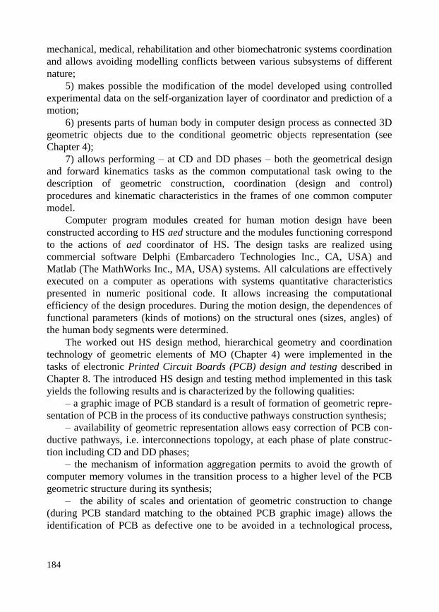
184
mechanical, medical, rehabilitation and other biomechatronic systems coordination
and allows avoiding modelling conflicts between various subsystems of different
nature;
5) makes possible the modification of the model developed using controlled
experimental data on the self-organization layer of coordinator and prediction of a
motion;
6) presents parts of human body in computer design process as connected 3D
geometric objects due to the conditional geometric objects representation (see
Chapter 4);
7) allows performing – at CD and DD phases – both the geometrical design
and forward kinematics tasks as the common computational task owing to the
description of geometric construction, coordination (design and control)
procedures and kinematic characteristics in the frames of one common computer
model.
Computer program modules created for human motion design have been
constructed according to HS aed structure and the modules functioning correspond
to the actions of aed coordinator of HS. The design tasks are realized using
commercial software Delphi (Embarcadero Technologies Inc., CA, USA) and
Matlab (The MathWorks Inc., MA, USA) systems. All calculations are effectively
executed on a computer as operations with systems quantitative characteristics
presented in numeric positional code. It allows increasing the computational
efficiency of the design procedures. During the motion design, the dependences of
functional parameters (kinds of motions) on the structural ones (sizes, angles) of
the human body segments were determined.
The worked out HS design method, hierarchical geometry and coordination
technology of geometric elements of MO (Chapter 4) were implemented in the
tasks of electronic Printed Circuit Boards (PCB) design and testing described in
Chapter 8. The introduced HS design and testing method implemented in this task
yields the following results and is characterized by the following qualities:
– a graphic image of PCB standard is a result of formation of geometric repre-
sentation of PCB in the process of its conductive pathways construction synthesis;
– availability of geometric representation allows easy correction of PCB con-
ductive pathways, i.e. interconnections topology, at each phase of plate construc-
tion including CD and DD phases;
– the mechanism of information aggregation permits to avoid the growth of
computer memory volumes in the transition process to a higher level of the PCB
geometric structure during its synthesis;
– the ability of scales and orientation of geometric construction to change
(during PCB standard matching to the obtained PCB graphic image) allows the
identification of PCB as defective one to be avoided in a technological process,

185
when the PCB orientation and the distance in relation to the video camera are
changed;
– in the process of pathways quality testing the standard and obtained PCB
images are compared not by continuous scanning of PCB image lines as in the
technologies already known, but only by scanning along the interconnection lines –
conductive pathways – with regard to their geometric representations; it allows the
reduction of both the comparison time and computer memory volumes.
Aed symbol construction of HS gave a formal basis for the descriptions of the
PCB geometric structure and the processes of its design and testing presented in
Chapter 8, and allowed creating the PCB conceptual model. Availability of coordi-
nator allowed performing the decision making tasks on its strata at both PCB con-
ceptual and detailed design phases. Algorithms of the given HS design technology
was applied in PCB production process of Horizont enterprise (Minsk, Belarus).
The use of Hierarchical Systems (HS) technology in conceptual design and
control of MCM (Manhole Cutting Machine) is presented in Chapter 9. Developed
conceptual model of the MCM system contains connected systemic models of
mechatronic subsystems, i.e. human – man-operator, computer control, visual
informatics, electronic – sensors, electromechanical – servo drives, and executive
mechanical (MCM tool, arm and its joints), presented in general aed formal basis
of HS. The MCM system structure, its dynamic presentation as the unit in its
technological environment, MCM environment – other objects and technological
units of the production process, and MCM control unit – ACOPOS controller –
were also described in this basis. MCM design and control functions were taken
into account owing to HS coordinator availability. MCM coordinator performs
coordination – design and control – tasks on its selection, learning and self-
organization strata.
The conceptual formal model of MCM machine presented in Chapter 9 is
coordinated with traditional systems of information presentation in mechatronics –
numeric, graphic and natural language forms. It was shown, that MCM conceptual
model presented in aed formal basis of HS is coordinated with general
requirements of design and control systems and allows easy transfer from
Conceptual Design phase to Detailed Design phase in MCM life cycle. It brings
new possibilities in creating a formal language for MCM and similar technological
machines conceptual design. Both MCM conceptual model creation and design
processes described in Chapter 9 were executed in the frames of the R&D project
maintained by the agreements between Bialystok University of Technology and
Promotech enterprise (Bialystok, Poland).
Therefore, the conceptual model of mechatronic objects being designed, the
design system and coordination – design and control – process are presented in aed
formal basis of HS in this book. In comparison with traditional models of mathe-
matics, artificial intelligence and widespread design methods (see Chapter 1) the

186
developed conceptual formal model contains connected descriptions of the de-
signed mechatronic object structure, its aggregated dynamic representation as a
unit in its environment, the environment model and the design&control system. All
the descriptions are connected by the coordinator which performs the design and
control tasks on its strata. Besides, the suggested aed technology of HS coheres
with traditional systems of information presentation in mechatronics: numeric,
graphic and natural language forms. Aed technology and HS design method are
also coordinated with general requirements of the design and control systems and
consider mechatronic subsystems of different nature – mechanical, electromechan-
ical, electronic, computer – in common theoretical basis.
Besides, aed technology and HS design method are an effective means of
mechatronic objects design and conceptual models creation. These models allow
an easy transfer from the conceptual design phase to a detailed design phase in the
mechatronic object’s life cycle and allow description of the design procedures in
the form of coordination strategies of HS. At the conceptual design phase, the
mechatronic subsystems of MS being designed are presented in the form of dynam-
ic system (ρ,φ) which is generalization of DE, automata and algebra systems. So,
the transition from the conceptual to the detailed design phase in the frames of the
HS design method suggested is convenient and requires concretization of the ab-
stract dynamic system only.
All the qualities mentioned above make the suggested HS design technology
more efficient in design tasks performing in comparison with widespread design
methods (see Chapter 1). The presented HS design method brings new informa-
tional means for the conceptual and detailed design of mechatronic systems.
The conceptual design method presented in this book has been also applied
to the design and control of other engineering objects [53, 113-117], in robotics [50,
54-58, 119-125, 141-142], biomechanics [55, 118] and mechatronics [49-51, 58,
126], in design tasks of industrial knowledge networks [23, 24], written text [127]
and natural language processing [8], and other tasks.
Some theoretical foundations and application results of the method presented
in this book were discussed with one of the authors of the theory of hierarchical
and dynamic systems Prof. Yasuhiko Takahara [2, 10], and one of the authors of
mathematical and computer aided systems theory Prof. Franz R. Pichler [138, 139].
The described HS conceptual design method was also implemented in R&D
projects with PROMOTECH enterprise (Bialystok, Poland), MTZ and HORI-
ZONT enterprises (Minsk, Belarus), EU projects ICIMS-NoE, AMETMAS-NoE,
DYCOMANS, ACAT Horizont 2020 project, grants and projects maintained by
KOSEF and NSF (South Korea), and others.

187
Acknowledgements
I would like to give special thanks to my parents Professor Anna Miatluk and Pro-
fessor Mikolaj Miatluk for always supporting and encouraging me.
I owe a great debt of gratitude to Professor Svetlana Novikava and Professor
Yasuhiko Takahara who put freely at my disposal their immense experience and
knowledge.
I would like to express my deep gratitude to my colleagues of Automatic
Control and Robotics department, Mechanical Engineering Faculty, Bialystok Uni-
versity of Technology, as well as to Prof. Jerzy Pokojski, Prof. Marek Gawrysiak
and Prof. Franz R. Pichler for much wise advice at the planning stage of this book.
I express my great gratitude to Professors Y.H. Kim, K. Kim, D. Pascault, N. Kru-
ger, H.G. Petersen, M. Diaz-Cabrera – my co-authors of our joint works where
some ideas of the presented HS design and control method were implemented.

188
References 1. Ullman D.G.: The mechanical design process, 4th ed., Singapore: McGraw-
Hill, 2010.
2. Mesarovic M.D., Macko D. and Takahara Y.: Theory of hierarchical multi-
level systems, Academic Press, New York, NY, 1970.
3. Miatliuk K.: Formal model of coordinator of two-level system, Belarus Acad-
emy of Science, Minsk, 1987, (in Russian).
4. Novikava S., Mialtiuk K., Gancharova S. and Kaliada W.: Aed construction
and technology in design, Proc. of 7th IFAC LSS Symposium, Pergamon,
London, 1995, pp. 379-381.
5. Novikava S., Miatluk K., et al.: Hierarchical systems in Aed realization,
Proc. of 9th IMACS Conference, Berkeley, USA, 1993, p. 71.
6. Novikava S., Miatliuk K., et al.: Mathematical and cybernetical means of
Aed theory, IEEE Int. Conference on Systems, Man and Cybernetics, Vol. 1-
4, China, 1996, pp. 2874-2879.
7. Novikava S., Miatluk K., et al.: Aed theory in hierarchical knowledge net-
works, Int. Journal Studies in Informatics and Control, Vol. 6 No. 1, 1997,
pp.75-85.
8. Novikava S., and Miatliuk K.: Hierarchical system of natural grammars and
process of innovations exchange in polylingual fields, Kybernetes, Emerald,
Vol. 36, No. 5/6, 2007, pp. 736-748.
9. Mesarovic, M.D. and Takahara, Y.: General systems theory: mathematical
foundations, Academic Press, New York, NY, 1975.
10. Mesarovic, M. and Takahara, Y.: Abstract Systems Theory, Springer, 1990.
11. Mialtiuk, K.: Coordination processes of geometric design of hierarchical
systems, Machine building and exploitation, WPB, Vol. 11, 2003, pp. 163-
78. (in Polish)
12. Moulianitis V.C., Aspragathos N.A. and Dentsoras A.J.: A model for concept
evaluation in design – an application to mechatronics design of robot grip-
pers, Mechatronics, Vol. 14, 2004, pp. 599–622.
13. Childs P.: Mechanical Design Engineering Handbook, Elsevier, Hardbound,
2013, 856 p.
14. Johnson J.: Designing with the Mind in Mind, Elsevier, 2014.
15. Liu C., Hildre H.P., Zhang H., Rølva T.: Conceptual design of multi-modal
products, Res. Engineering Design, Springer, Vol. 26, 2015, pp. 219–234.

189
16. Hudspeth M.: Conceptual Design in Product Data Management, Design En-
gineering Technology News, Desktop Engineering, February 1, 2008.
17. French M.J.: Conceptual Design for Engineers, Springer, 3rd Edition, 1999.
18. Analyzing requirements and defining Microsoft.net solution architectures,
Microsoft Press, 2003.
19. FLH Project Development and Design Manual, Conceptual Studies and Pre-
liminary Design, US Department of Transportation, 2014,
(http://flh.fhwa.dot.gov/resources/).
20. Pokojski J. and Szustakiewicz K.: Towards an aided process of building a
knowledge based engineering applications, Machine Dynamics Problems,
Vol.33, No.3, 2009, pp. 91-100.
21. Papiernik K., Grabska E., Borkowski A.: On applying model-driven engi-
neering to conceptual design, Machine Dynamics Problems, Vol.31, No.3,
2007, pp.58-65.
22. Pahl, G., Beitz, W., Feldhusen, J. and Grote, K.-H.: Engineering design: a
systematic approach, Springer, 3d edition, 2007.
23. Miatliuk K., et al.: The coordinating system of knowledge network for tractor
and automobile industry, 5th Int. Conference on Technology, Policy and In-
novation, Delft, Netherland, 2001, pp.292-293.
24. Novikava S., Miatliuk K., Pavlushchenko A.: Knowledge network for ma-
chine-bulding industry coordination, Proc. of the 16th Int. Conference on
Systems Science ICSS, Wrocław, 2007, pp. 413-420.
25. Bryant, C.R., et al.: Concept generation from the functional basis of design,
Proc. of Int. Conference on Engineering Design (ICED 2005), Melbourne,
Australia, 2005.
26. Gero, J.S. and Kannengiesser, U.: A function–behaviour–structure ontology
of processes, Artificial Intelligence for Engineering Design, Analysis and
Manufacturing, Vol. 21 (4), 2007, pp. 379–391.
27. Borgo, S., et al.: A formal ontological perspective on the behaviors and func-
tions of technical artifacts, Artificial Intelligence for Engineering Design,
Analysis and Manufacturing, Vol. 23 (1), 2009, pp.3–21.
28. Yan X.T. and Zante R.: A mechatronic design process and its application,
Mechatronics in Action, ed. D. Bradley and D.W. Russell, Springer, 2010,
pp.55-70.
29. Giergiel J., Kurc K., Giergiel M.: Mechatronic design of the inspection ro-
bots, WPR, 2010 (in Polish)
30. Ralph P. and Wand Y.: A proposal for a formal definition of the design con-
cept, Design Requirements Workshop, LNBIP, Springer, 2009, pp. 103-136.
31. Gu C., Hu J., Peng Y., Li S.: FCBS model for functional knowledge repre-
sentation in conceptual design, Journal of Engineering Design, Vol.23 (8),
2012, pp.577-596.

190
32. Takahara, Y and Mesarovic, M.: Organization structure: cybernetic systems
foundation, Kluwer Academic Publishers, New York, 2003.
33. Novikava S., Miatliuk K., et al.: The Structure and the Dynamics of Infor-
mation in Design Systems, Proc. of the 7th Int. Conference on Engineering
Design, ICED'90, Dubrovnik, Vol. 2, 1990, pp. 946-953.
34. Stroud I.: Boundary Representation Modelling Techniques, Springer, 2006.
35. Um D.: Solid modeling and applications, Springer Switzerland, 2016.
36. Wang Y., Nnaji B.O.: Geometry-based semantic ID for persistent and in-
teroperable reference in feature-based parametric modeling. Computer Aided
Design, Vol. 37, Issue 10, Elsevier, 2005, pp. 1081-1093.
37. Baerentzen, J. A., Gravesen, J., Anton, F., and Aanaes, H.: Guide to compu-
tational geometry processing. Polygonal meshes. Springer London, 2012, pp.
83- 97.
38. Selimovic I.: New bounds on the magnitude of the derivative of rational Bé-
zier curves and surfaces, Computer Aided Geometric Design, Vol. 22, Issue
4, Elsevier, 2005, pp. 321-326.
39. Nizeki M.: The principle of duality in data structures and Euler operators of
Solid Modelers, 3rd Int. Conf. on Design Engineering and Science, Czech
Republic, 2014, pp. 41-46.
40. De Floriani L.: Digital geometry algorithms, ed. Brimkov V. and Barneva
R., Vol. 2, Dordrecht, Springer Netherlands, 2012.
41. Cano P., Torres J.: Representation of polyhedral objects using SP-octrees.
Journal of WSCG, Vol.10, 2002, pp.95-101.
42. Nemcowa D.: Three-dimensional representation of raster images. Technical
University of Wien, 2000.
43. Bayro-Corrochano E., Scheuermann G.: Geometric algebra computing,
Springer London, 2010.
44. Höllig K. and Hörner J.: Approximation and modeling with B-splines, SIAM,
2013.
45. Sederberg T. W.: Computer Aided Geometric Design, BYU, 2014, 262 p.
46. Wolniakowski A., Koziol P., and Miatliuk K.: Generating trajectory for 5
DoF serial link CNC machine with kinematic constraints, 15th IEEE Int.
Carpathian Control Conference, Czech Republic, 2014, pp. 689-694.
47. GSC Associates, (www.gscassociates.com)
48. Lebesgue H. L.: Measure and the integral, Holden-Day, 1966.
49. Miatliuk K.: Conceptual model in the formal basis of hierarchical systems for
mechatronic design, Cybernetics and Systems, Taylor& Francis, Vol. 46, Is-
sue 8, 2015, pp.666-680.
50. Miatluk K., Siemieniako F.: Theoretical basis of coordination technology for
systems design in robotics, Proc. of the 11th IEEE Int. Conference on Meth-
191
ods and Models in Automation and Robotics MMAR, Międzyzdroje, Poland,
2005, pp.1165-1170.
51. Mialtiuk K., Kim Y.H., Kim K., Siemieniako F.: Use of hierarchical system
technology in mechatronic design, Mechatronics, Vol. 20, No.2, Elsevier,
2010, pp. 335-339.
52. Miatliuk K.: Geometrical representation based on the hierarchical systems
technology, 14th Int. Conf. on Computer Aided Systems Theory: Eurocast
2013, Las Palmas, Spain, 2013, pp. 59-62.
53. Miatliuk K., Mystkowski A.: Realization of coordination technology of hier-
archical systems in design of active magnetic bearings system, Journal of
Theoretical and Applied Mechanics, Vol. 53, 3, 2015, pp. 711-722.
54. Miatliuk K.: Conceptual design of parallel stuart robot using hierarchical
systems technology, 15th Int. Conf. on Computer Aided Systems Theory: Eu-
rocast 2015, Las Palmas, Spain, 2015, pp.227-228.
55. Miatliuk K., Kim Y. H: Hierarchical systems technology in the coordination
of biomechanical motion, Proc. IEEE SICE-ICASE International Joint Conf.
on Control, Automation and Systems ICCAS 2006, Busan, South Korea,
2006, pp. 244-249.
56. Miatliuk K.: Coordination technology in design of biologically inspired ro-
bot, Machine Dynamics Problems, Vol.33, No. 3, 2009, pp.70-78.
57. Miatliuk K., Siemieniako F.: Hierarchical systems technology in design of
walking robot, Int. J. of Applied Mechanics and Engineering, Vol.15, nr 3,
2010, pp. 793-797.
58. Miatliuk K., Kim Y.H.: Application of hierarchical systems technology in
conceptual design of biomechatronic system, Advances in Intelligent Systems
and Computing, Vol. 240, Springer, 2014, pp 77-86.
59. Bargar, W. L., Bauer A. and Börner M.: Primary and revision total hip re-
placement using the ROBODOC(R) system, Clinical Orthopaedics and Re-
lated Research, Vol. 354, 1998, pp. 82- 91.
60. Catani F., and Stefano Zaffagnini S.: Knee surgery using computer assisted
surgery and Robotics, ESSKA Luxembourg, 2013.
61. Kim Y.H. and Minh H.L.: A laboratory-level surgical robot system for mini-
mal invasive surgery (MIS) total knee arthroplasty, International Journal of
Precision Engineering and Manufacturing, 2011, Vol. 12, No 2, pp. 237-242.
62. Tsuji S., Tomita T., Fujii M., Laskin, R., Yoshikawa H., Sugamoto K.: Is
minimally invasive surgery - total knee arthoroplasty truly less invasive than
standard total knee arthroplasty? The Journal of Arthroplasty, Vol. 25, No. 6,
2010, pp. 970-976.
63. Mako Surgical Corp., Makoplasty system, http://www.makosurgical.com
64. Acrobot Sculptor, http://www.acrobot.com
65. Curexo, Inc., ROBODOC system, http://www.curexo.com

192
66. Bioloid Comprehensive Kit, Robotis, Korea, www.robotis.com
67. Buratowski T., Giergiel M., Uhl T.: Mechatronic design of the six legged
walking robots, 21st Int. Conf. on CAD\CAM, Robotics and Factories of the
Future, Krakow, 2005.
68. Feczko J., Manka M., Krol P., Giergiel M., Uhl T., Pietrzyk A.: Review of
the modular self reconfigurable robotic systems, 10th Int. Workshop on Robot
Motion and Control, RoMoCo 2015, Poznań, Poland, 2015, pp. 182-187.
69. Bartoszewicz A.: Hanging robots – new trend in mechatronics development,
Mechatronics. Regional Technological Foresight, Lodź, 2008, pp. 133-134
(in Polish).
70. Pazderski D., and Kozłowski K.: Motion control of a skid-steering robot us-
ing transverse function approach – experimental evaluation, 10th Int. Work-
shop on Robot Motion and Control, RoMoCo 2015, Poznań, Poland, 2015,
pp. 72-77.
71. Moulianitis V.C., and Aspragathos N. A.: IT and Mechatronics in industrial
robotic workcell design and operation, in: Encyclopedia of Information Sci-
ence and Technology, IGI Global, 2015, pp. 440-455.
72. Miatliuk K., Kim Y.H., Kim K.: Motion control based on the coordination
method of hierarchical systems, J. of Vibroengineering, Vol.11, No 3, 2009,
pp. 523-529.
73. Miatliuk K., Gosiewski Z., Siemieniako F.: Coordination technology in the
assembly operations design, Proc. IEEE SICE-ICASE International Joint
Conf. on Control, Automation and Systems ICCAS’2006, Busan, South Ko-
rea, 2006, pp. 2243-2246.
74. SolidWorks, http://www.solidworks.com/
75. Pandy, M.G.: Computer modeling and simulation of human movement, An-
nual review of biomedical engineering, Vol. 3, 2001, pp. 245-273.
76. Park, W., et. al.: A computer algorithm for representing spatial–temporal
structure of human motion and a motion generalization method, Biomechan-
ics, Vol. 38, 2005, pp. 2321-2329.
77. Azevedo et al.: Bipedal locomotion: toward unified concepts in robotics and
neuroscience, Biological Cybernetics, Vol. 96, 2007, pp. 209–228.
78. Yu F., Xue Q., Liu M.: Virtual human motion design and ergonomics analy-
sis in maintenance simulation, Advances in Applied Digital Human Modeling
and Simulation, Springer, Vol. 481, 2016, pp. 65-74.
79. Vaughan, C.L.: Theories of bipedal walking: an odyssey, Biomechanics, Vol.
36, 2003, pp. 513-523.
80. Miatliuk K., Kim Y.H., Kim K.: Human motion design in hierarchical space,
Kybernetes, Emerald, Vol.38, No.9, 2009, pp.1532-1540.
81. Steger C., et al.: Machine vision algorithms and applications. Wiley, 2008.

193
82. Laranjeira L. et al.: Tool for Fault Extraction in PCBs, IEEE Test Workshop,
Portugal, 2000.
83. Verma, A.: Optimizing test strategies during PCB design for boards with
limited ICT access, 27th Annual IEEE/SEMI International, IEMT Symposium,
2002, pp.364-371.
84. McDaniel J., Grissom D., Brisk P.: Multi-terminal PCB escape routing for
digital microfluidic biochips using negotiated congestion, 22nd IFIP/IEEE In-
ternational Conference on Very Large Scale Integration (VLSI-SoC), Mexi-
co, 2014, pp. 219-224.
85. Duvvury C., Gossner H.: System level ESD co-design, Wiley, 2015.
86. Mehri M., Masoumi N.: Statistical Prediction and Quantification of Radiated
Susceptibility for Electronic Systems PCB in Electromagnetic Polluted Envi-
ronments, IEEE Transactions on Electromagnetic Compatibility, Issue 99,
2016, pp.1-11.
87. Aysu A., Gaddam S., Mandadi H., Pinto C., Wegryn L., Schaumont P.: A
design method for remote integrity checking of complex PCBs, Design, Au-
tomation and Test in Europe Conference, 2016, pp.1517-1522.
88. Miatliuk K., Diaz-Cabrera M.: Application of hierarchical systems technolo-
gy in design and testing of circuit boards, Lecture Notes in Computer Sci-
ence, Springer, Vol. 8112, 2013, pp. 521-526.
89. Chameleon video camera, https://www.ptgrey.com/chameleon3-usb3-vision-
cameras
90. Grasshopper video camera, https://www.ptgrey.com/grasshopper3-usb3-
vision-cameras
91. Matlab, https://www.mathworks.com
92. MCM machine, http://www.promotech.eu/products/en/welding_cutting/doc/
93. Kozioł P., Kuklinski K., Wołniakowski A., Miatliuk K.: Solution for inverse
kinematics of 5 DoF serial link MCM machine, Solid State Phenomena,
Trans Tech Publ., 2013, pp. 53-58.
94. Miatliuk K.: Conceptual model for design and control of MCM machine,
17th IEEE Int. Carpathian Control Conference, Slovakia, 2016, pp. 490-493.
95. Automation Studio, http://www.br-automation.com/cps/rde/xchg/br-productcatalogue/
96. B&R automation, www.br-automation.com
97. Ellekilde L.P., Jørgensen J.A.: Robwork: a flexible toolbox for robotics re-
search and education, Int. Symposium on Robotics, 2010, pp. 800–806.
98. RobWork, http://www.robwork.dk/jrobwork/
99. https://www.br-automation.com/en/products/motion-control/acopos/
100. https://www.br-automation.com/pl/produkty/technologia-
bezpieczenstwa/x67-system/
101. Matlab simulink, https://www.mathworks.com

194
102. Krysiak B., and Kozlowski K.: Kinematic singularities avoidance for the
planar three–link nonholonomic manipulator, 10th Int. Workshop on Robot
Motion and Control, RoMoCo 2015, Poznań, Poland, 2015, pp. 252-256.
103. Martowicz A., Ciszewski M., Buratowski T., Gallina A., Rosiek M., Seweryn
K., Teper W., Zwierzyński A.J., Uhl T.: Mechatronic approach in application
to solution of research and design problems, Mechatronics, Vol. 36, 2016,
pp. 1–17.
104. Gawrysiak M.: Systemic analysis of mechatronic devices, WPB, Bialystok
2003 (in Polish).
105. Petko M., Karpiel G.: Mechatronic design of a parallel robot for milling, Sol-
id State Phenomena, Vol. 198, 2013, pp. 21-26.
106. Awrejcewicz J., Szewczyk R., Trojnacki M., Kaliczyńska M. (eds.): Mecha-
tronics: ideas for industrial applications, Springer, 2015.
107. Ciszewski M., Buratowski T., Giergiel M., Małka P., Kurc K.: Virtual proto-
typing, design and analysis of an in-pipe inspection mobile robot, J. of Theo-
retical and Applied Mechanics, Vol. 52, 2, 2014, pp. 417-429.
108. Jablonski R., Turkowski M., Szewczyk R. (eds.): Recent advances in mecha-
tronics, Springer, 2007.
109. Brezina T., Jablonski R. (eds.): Recent advances in mechatronics, Springer,
2010.
110. Zeghloul S., et al. (eds.), Robotics and Mechatronics, Springer, 2016.
111. Van Der Veen G., et al.: Topology optimization for the conceptual design of
precision mechatronic systems, Proc. 30th Annual Meeting of the American
Society for Precision Engineering ASPE, 2015, pp.136-141.
112. Bruno S., et al.: The conceptual design of a mechatronic system to handle
bedridden elderly individuals, Sensors, Vol. 16, Issue 5, 2016.
113. Kulesza Z., Miatluk K., Miatluk M.: Modelowanie i obliczenia dynamiki
pneumohydraulicznych układów napędowych: in; Dynamika pneumatycz-
nych układów napędowych, ed. F. Siemieniako, WPB, Białystok, 2007, pp.
191-226.
114. Lukaszewicz A., Miatliuk K.: Reverse engineering approach for object with
free-form sufraces using standard surface-solid paramteric CAD system, Sol-
id State Phenomena, Vol. 147-149, 2009, pp. 706-711.
115. Miatliuk K., Gosiewski Z., Siemieniako F.: Theoretical means of hierarchical
systems for design of magnetic bearings, 8th IFToMM Int. Conference on
Rotor Dynamics, Seoul, South Korea, 2010, pp. 1035-1039.
116. Diaz-Cabrera M., Cabrera-Gámez J., Aguasca-Colomo R., Miatliuk K.: Pho-
togrammetric analysis of images acquired by an UAV, Lecture Notes in
Computer Science, Springer, Vol. 8112, 2013, pp. 109-116.

195
117. Miatliuk K., Holewa K., Nawrocka A.: Conceptual design of BCI in the for-
mal basis of hierarchical system, IEEE 15th Int. Carpathian Control Confer-
ence: ICCC’2014, Czech Republic, 2014, pp. 336-341.
118. Miatliuk K.: Interaction modeling of biomechanical object and its environ-
ment, 4th Int. Symposium of Measurement, Analysis and Modelling of Human
Functions, Czech University of Life Sciences, Prague, 2010, pp. 57-58.
119. Miatliuk K.: Coordination technology in design of humanoid robots, XII
Polish - Ukrainian Conference on CAD machinery design, Warszawa, 2009,
pp. 35-36.
120. Popovic M., Kootstra G., Jørgensen J. A., Kuklinski K., Miatliuk K., Kragic
D., Kruger N.: Enabling grasping of unknown objects through a synergistic
use of edge and surface information, International Journal of Robotics Re-
search, SAGE, 31(10), 2012, pp. 1190–1213.
121. Wolniakowski A., Miatliuk K., Krüger N., Rytz J.A.: Automatic evaluation
of task-focused parallel jaw gripper design, Lecture Notes in Artificial Intel-
ligence, Springer, Vol. 8810, 2014, pp. 77-86.
122. Wolniakowski A., Jorgensen J.A., Miatliuk K., Petersen H.G., Kruger N.:
Task and context sensitive optimization of gripper design using dynamic
grasp simulation, 20th IEEE Int. Conference on Methods and Models in Au-
tomation and Robotics, MMAR, Międzyzdroje, 2015, pp. 29-34.
123. Kuklinski K., Savarimuthu T.R., Fischer K., Beck R., Krüger N., Miatliuk
K., Kirstein F., Marhenke I., Wieschen M.V., Sølvason D.: A novel tele-
operation device allowing for dynamic switching between control points dur-
ing learning from demonstration, 10th IEEE Int. Workshop on Robot Motion
and Control: RoMoCo’15, Poznan, 2015, pp. 314-318.
124. Wolniakowski A., Gams A., Chrysostomou D., Madsen O., Miatliuk K., Pe-
tersen H.G., Hagelskjær F., Buch A.G., Ude A., Krüger N.: Compensating
pose uncertainties through appropriate gripper finger cutouts, 12th Int. Conf.
Mechatronic Systems and Materials MSM’2016, Bialystok, Poland, 2016,
p.27.
125. Miatliuk K., Pascault D.: Control of Stewart parallel structure with concur-
rent learning, 12th Int. Conf. Mechatronic Systems and Materials, Bialystok,
Poland, 2016, p. 91.
126. Miatliuk K., Kim Y. H., Siemieniako F.: Informational basis for mechatronic
systems design, Proc. of the 3d Asia Int. Symposium on Mechatronics:
AISM’2008, Sapporo, Japan, 2008, p. 538-543.
127. Miatliuk K., Diaz-Cabrera M.: Geometrical representation of written text
elements using hierarchical systems technology, 15th Int. Conf. on Computer
Aided Systems Theory: Eurocast’2015, 2015, pp.19-20.

196
128. Sapinski B.: Simulation of an MR squeeze-mode damper for an automotive
engine mounting, 17th IEEE Int. Carpathian Control Conference, ICCC
2016, Slowakia, 2016, pp. 641-644.
129. Tisch M., Hertle C., Abele E., Metternich J., Tenberg R.: Learning factory
design: a competency-oriented approach integrating three design levels, Int.
Journal of Computer Integrated Manufacturing, Vol. 29, Issue 12, 2016, pp.
1355-1375.
130. Weiss Z., Pankowski M., Kowalski M.: Reverse engineering at VIDA centre.
Virtual Design and Automation, WPP, Poznań, 2005, pp. 219-226.
131. Ozkan B.: Investigation of the usefulness of the linear homing guidance law
for the motion planning of mechatronic systems, 17th IEEE Int. Carpathian
Control Conference, ICCC 2016, Slowakia, 2016, pp.539-544.
132. Sobieszczanski-Sobieski J., Morris A., J.L.van Tooren M.: Multidisciplinary
design optimization supported by knowledge based engineering, John Wiley
& Sons, 2015.
133. Gausemeier J., Ramming F.J., Schafer W. (eds.): Design methodology for
intelligent technical systems, Springer, 2014.
134. Kühn A., Dumitrescu R., Gausemeier J.: Managing evolution from mechatron-
ics to intelligent technical systems, Jurnal Teknologi, 76 (4), 2015, pp. 13-18.
135. Petko M., Karpiel G., Gac K., Góra G., Kobus K., Ochoński J.: Trajectory
tracking controller of the hybrid robot for milling, Mechatronics, Vol. 37,
2016, pp. 100–111.
136. Rohatyński R.: Conceptual design within the product development process.
Virtual Design and Automation, WPP, Poznań, 2005, pp. 71-82.
137. Wróbiel J., Ruschitzka M., Suchodolski A.: Ontologically-based approach for
knowledge representation for stamping die applications, Computer Aided De-
sign & Applications, No 6(3), 2009, pp. 281-289.
138. Pichler F.: Mathematical system theory, dynamic structures, Berlin-New
York, Walter de Gruyter, 1975.
139. Pichler F., Schwärtzel H.: Computer-aided systems theory. methods in model-
ling, Springer, 1992.
140. Miatliuk K.: Geometric design of hierarchical objects by coordinator meth-
od, Doctoral thesis, Krakow, 2006.
141. Wolniakowski A., Miatliuk K., Gosiewski Z., Bodenhagen L., Petersen H.G.,
Jørgensen J.A., Krüger N.: Task and context sensitive gripper design learning
using dynamic grasp simulation, J. of Intelligent and Robotic Systems,
Springer, Vol, 87, Issue 1, 2017, pp 15–42.
142. Wolniakowski A., Gams A., Kramberger A., Chrysostomou D., Madsen O.,
Miatliuk K., Buch A., Ude A., Petersen H.G., Krüger N.: Compensating pose
uncertainties through appropriate gripper finger cutouts, Acta Mechanica et
Automatica, 2017.