oil shocks and regional heterogeneity: the case of japan · legislation in euro area countries. vu...

1

Oil shocks and regional heterogeneity: The case of Japan

Hayato Nakata*

Meisei University

Tuan Khai Vu**

Hosei University

June, 2018

(Preliminary)

Abstract

This paper addresses the question of how the effects of oil shocks on different economies are affected

by their heterogeneity. We take up the Japanese regional economies as a case study and use a structural

VAR model and a panel VAR model as the analytical framework. We find that the effects of oil price

shocks on the Japanese regional economies are closely related to various natural and socio-economic

characteristics of those regions. More specifically, in the presence of a surge in the oil price caused by

an oil demand shock originated from the global real economic activity or an oil market specific demand

shock, output is more negatively affected and the price level rises more in a region with colder winter,

or with lower population density, or with a higher share of petroleum and coal products in total value

added. In addition, the effects of oil price shocks also depend on the share of transport equipment

industry, one of the key industries of Japan: The more a region is specializing in this industry the more

its output and the less its price level respond to oil demand shocks.

Keywords: oil price fluctuations, Japanese regional economies, panel VAR.

JEL codes: F41, Q43, R11.

* Associate Professor. School of Economics, Meisei University. Mailing address: 2-1-1 Hodokubo, Hino-shi, Tokyo

191-8506, Japan. E-mail: hnakata econ.meisei-u.ac.jp. ** Professor. Faculty of Economics, Hosei University. Mailing address: 4342 Aihara-machi, Machida-shi, Tokyo 194-

0298, Japan. E-mail: vu.tuankhai meisei-u.ac.jp.

2

1. Introduction

This paper studies the effects of world-market oil price fluctuations on the regional

economies of Japan and analyzes how these effects are related to various types of heterogeneity across

these regions.

Since 2000, the sharp rise in the world-market oil price has triggered a large number of

empirical studies aiming to analyze effects of oil price shocks on the macroeconomy. Some of these

studies look at the differences in the effects of oil price shocks across countries (see, e.g., Peersman

and Robays (2009) and Vu and Nakata (2018)), or across regions within the same country (see our

previous study Vu and Nakata (2016)).

On the other hand, very few papers investigate the factors behind these differences in the

effects of oil price shocks across countries or across regions. Peersman and Robay (2009) examine the

relationship between the impacts of oil price on wages, or GDP deflator and strictness of employment

legislation in Euro area countries. Vu and Nakata (2018) find a negative relationship between the

contributions of oil price shocks to the variances of CPI and IIP and the oil production/consumption

ratio in ASEAN countries. Using regional data of Japan, Vu and Nakata (2016) analyze the relationship

between the effects of oil price on CPI, IIP and the climate condition and industrial structure in these

regions. However, a shortcoming of these studies is that they cannot carry out formal statistical tests

due to the lack of enough observations in the sample used, and as a result, they have to rely on

investigation using correlation coefficient or scatter diagram.

The present paper aims to overcome this problem by using a Japanese prefectural-level panel

data set. Our data set consists of data on 47 prefectures of Japan and spans a period of over more than

30 years. We analyze the effects of oil price fluctuations on regional economies in Japan, and examine

how these regional effects are related to various indicators on regional heterogeneity.

It is worth noting that Japan is suitable for an analysis of the regional differences in the

effects of oil price shocks because regions in Japan are quite diverse in several dimensions. For

example, the Japanese archipelago stretches over 3000 kilometers from northeast to southwest,

possessing a large difference in climate and geographical conditions between regions. In addition,

there is also considerable regional heterogeneity in economic structure. It is also worth noting that, for

many indicators on the regional heterogeneity in Japan, the data are available to us. Therefore, using

prefectural-level data of Japan with such features, our approach can analyze the regional heterogeneity

in the effects of oil price shocks in much more detail and in a more rigorous way.

We employ a panel vector autoregressive (VAR) model which includes three types of oil

shocks as exogenous variables, and economic variables such as the price level (CPI) and output (IIP)

of each prefecture as endogenous variables. The oil shocks here are identified using the framework of

Kilian (2009) before being used in the panel VAR. The use of a panel VAR model enables us to have

a much larger sample size, and thus increase the precision of the estimation. In investigating the factors

3

affecting the dynamic responses of economic variables in each prefecture to oil price shocks, we focus

on climate condition such as regional winter temperature, geographical condition such as population

density, and each region’s specialization coefficient in transportation equipment industry, an industry

which is especially important to Japanese economy, and in petroleum and coal products industry,

which uses crude oil as an input in production. By introducing the interaction terms between oil price

shocks and these factors, we can verify the relationship between regional factors and the effects of oil

price shocks.

The rest of the paper is structured as follows. The next two sections explain the empirical

methodology and data used in the study. Section 4 provides the results and analysis. The last section

concludes the paper.

2. Empirical methodology

Our study adopts a two-step approach to analyze the relationship between the effects of oil

price on CPI, IIP and the regional characteristics. At the first stage, we identify oil shocks via a

structural VAR. At the second stage, we use a panel VAR to estimate the effects of structural shocks

on regional CPI, IIP and the regional characteristics. Below we will describe each of these VARs in

details.

The VAR system in the first stage includes three variables, namely, oil production, global

economic activity, and oil price. Regarding the identification scheme, we employ the contemporaneous

zero restrictions of a recursive VAR following Kilian (2009). The contemporaneous zero restrictions

imply the following Cholesky decomposition of the covariance matrix of the residuals of the reduced-

form VAR.

𝑢𝑡 = [

𝑢𝑝𝑟𝑜𝑑,𝑡

𝑢𝑟𝑒𝑎𝑙,𝑡

𝑢𝑝𝑜𝑖𝑙,𝑡

] = [𝑎11 0 0𝑎21 𝑎22 0𝑎31 𝑎32 𝑎33

] [

𝜀𝑜𝑖𝑙𝑠𝑢𝑝,𝑡

𝜀𝑎𝑔𝑔𝑑𝑒𝑚,𝑡

𝜀𝑜𝑠𝑝𝑒𝑐,𝑡

] (1)

This scheme has the following implications about the relationship between variables: (i) Current oil

production is not affected by global economic activity and oil price in the same month; (ii) current

global economic activity is affected by oil production, but not by oil price in the same month; and (iii)

oil price is affected by oil production and global economic activity in the same month. With this

scheme, we can decompose oil price fluctuations into three types of structural components, namely,

oil supply shock, oil demand shock, and oil market specific demand shock.

The panel VAR in the second stage is represented by a system of linear equations as follows:

𝑌𝑖𝑡 = 𝑌𝑖𝑡−1𝐴1 + 𝑌𝑖𝑡−2𝐴3 + ⋯ + 𝑌𝑖𝑡−𝑝+1𝐴𝑝−1 + 𝑋𝑖𝑡𝐵1 + ⋯ + 𝑋𝑖𝑡−𝑞𝐵𝑞 + 𝜂𝑖 + 𝑒𝑖𝑡 (2)

4

for 𝑖 ∈ {1,2, ⋯ 𝑁}, 𝑡 ∈ {1,2, ⋯ , 𝑇𝑖}

where 𝑌𝑖𝑡 is a 1 × 𝑘 vector of endogenous variables, 𝑋𝑖𝑡 is a 1 × 𝑙 vector of exogenous variables,

𝜂𝑖 and 𝑒𝑖𝑡 are 1 × 𝑘 vectors of fixed effects and idiosyncratic errors, respectively, and 𝑝, 𝑞 are the

lag lengths of 𝑌𝑖𝑡 and 𝑋𝑖𝑡 . About the idiosyncratic errors, we assume that E[𝑒𝑖𝑡] = 0, 𝐸[𝑒𝑖𝑡, 𝑒𝑖𝑡] = Σ,

𝐸[𝑒𝑖𝑡, 𝑒𝑖𝑡] = 0 𝑓𝑜𝑟 𝑎𝑙𝑙 𝑡 > 𝑠.

In the panel VAR in (2), endogenous variables include the two variables: Index of Industrial

Production (IIP) and Consumer Price Index (CPI). Exogenous variables include the three types of

shocks (oil supply shock, aggregate demand shock, and oil price specific shock) estimated in (1), the

interaction terms of the structural shocks and the four variables representing the characteristics of each

region, namely, the share of transportation equipment industry in total value added, the share of

petroleum and coal products industry in total value added, the average temperature during winter

season, and population density. Thus, there are twelve interaction terms in total. In our panel VAR

analysis, the coefficients of these interaction terms are our main interest since these coefficients

capture the relationship between the regional characteristics and the effects of oil price on CPI and IIP.

We can judge the significance of these relationships based on the z-value results obtained for the

coefficients of interaction terms. In this regard, we believe that our approach is superior to the approach

used by previous studies in the literature which is merely splitting the sample into sub-samples.

Our estimation strategy is as follows. In order to remove the fixed effects, we adopt forward

orthogonal deviation (FOD) transformation. With FOD transformation, deviations from the average

of all available future observations are subtracted from each variable. We then estimate the transformed

the panel VAR model with System GMM estimation as proposed by Arellano and Bover (1995). This

method enables us to improve efficiency in estimation.

About the lag length in the panel VAR, we set p=12 taking into the fact that the data we use

are monthly. We set a lag length of three month for the exogenous variables.

To avoid estimating too many parameters, we do not include all variables on the regional

characteristics at once, but instead, we include each of them one by one in the estimation of the panel

VAR. Thus, there are a total of twelve regression equations being estimated.

3. Data

In this study, we use monthly data of the period 1976:1-2016:12, except for the regional

characteristic variables for which we use annual, or sample period average data in same period. For

the oil production, we obtain world oil production data from website of U.S. Energy Information

Administration (EIA). As for a measure of global real economic activity, we use the index constructed

by Lutz Kilian which we downloaded from his website. Oil price data is also taken from EIA website,

5

and is the crude oil acquisition cost by refiner in the US (dollars per barrel).

For the panel VAR analysis, we use prefectural level data in Japan with 47 prefectures in

total. Data of index of industrial production (IIP), and consumer price index (CPI) are taken from

Nikkei-NEEDS-CDCIs database. Annual data of the share of transportation equipment industry in

value added, and share of petroleum and coal products industry in value added are from census of

manufactures. As for temperature of winter, we use the 1980-2011 average temperature data in

prefectural capitals during winter season (from December to February) which is downloaded from

website of Japan Meteorological Agency. Annual data of population density are calculated from total

population and total area (𝑘𝑚2), among which the former data is taken from website of Ministry of

Internal Affairs and Communications.

4. Estimation results and analysis

This section provides the estimation results obtained using the panel VAR. Here, to save

space, we report only results about exogenous variables, i.e., oil shocks and regional characteristics.

These results are shown in Tables 1-4.

We start by looking at the coefficients of structural shocks. In the case of the oil supply shock

(𝑆𝑌𝑡), a positive shock increases IIP and decreases CPI significantly. These signs are consistent with

conventional economic theory because oil is used as an input in production and here the positive oil

supply shock raises the supply of oil reducing its price. In the case of the oil demand shock (𝐷𝐸𝑡), a

positive shock also increases IIP and CPI significantly and this result is also consistent with theory. As

for the oil market specific demand shock (𝑂𝐼𝐿𝑡), a positive shock increases IIP and CPI significantly.

Conventional economic theory predicts that (positive) oil market specific demand shocks increase CPI,

meanwhile the effects of these shocks on IIP depend on economic structure. Our results here are

consistent with previous studies, e.g., Vu and Nakata (2018), Iwaisako and Nakata (2017), Fukunaga,

Hirakata and Sugo (2009). One interpretation of these results is that oil market specific demand shocks

are news shocks reflecting changes in the expectations about the future growth of the world economy.

On the other hand, Vu and Nakata (2018) propose an alternative interpretation which is that oil market

specific demand shocks are demand shocks that occur at first in the oil industry or a small number of

related industries, and then over time spread to other industries.

Next, we look at the coefficients of the interaction terms. These coefficients are the main

interest of our study because the show how the regional heterogeneity in various characteristics affects

the differences in the effects of oil price shocks across regions.

Table 1 shows the results for the share of transport equipment industry (𝑆ℎ𝑎𝑟𝑒𝑇𝑟𝑎𝑛𝑠𝑡). In

Panel A of this table, which displays the effects on IIP, we can see that the coefficients of the interaction

terms of 𝐷𝐸𝑡 and 𝑆ℎ𝑎𝑟𝑒𝑇𝑟𝑎𝑛𝑠𝑡 take on significantly positive values at the lag lengths of one, two,

6

and three, while the coefficients of the interaction terms of 𝑂𝐼𝐿𝑡 and 𝑆ℎ𝑎𝑟𝑒𝑇𝑟𝑎𝑛𝑠𝑡 take on

significantly positive values at two and three lags. These results imply that, other things equal, the

more a region is specializing in the transport equipment industry, the more its output will increase in

response to a shock that raises global real economic activity and thus the demand for oil in the world

market.

In Panel B of Table 1, which displays the effects on CPI, we observe that the coefficient of

the interaction terms of 𝐷𝐸𝑡 and 𝑆ℎ𝑎𝑟𝑒𝑇𝑟𝑎𝑛𝑠𝑡 is significantly negative at one lag, implying that,

ceteris paribus, the more a region is specializing in the transport equipment industry, the less its price

level is affected by oil demand shocks. Regarding this result, our interpretation is that 𝑆ℎ𝑎𝑟𝑒𝑇𝑟𝑎𝑛𝑠𝑡

is highly positively correlated with the development of industry in a region, so the higher is

𝑆ℎ𝑎𝑟𝑒𝑇𝑟𝑎𝑛𝑠𝑡 in a region, the more goods (including consumption goods) the region can produce, the

less it is dependent on goods produced from other regions, and thus the smaller transportation costs it

needs to bear in importing goods from other regions, and therefore the less its CPI are affected by oil

shocks.

Table 2 shows the results for the share of petroleum and coal products in total value added

(𝑆ℎ𝑎𝑟𝑒𝑃𝑒𝑡𝑟𝑜𝐶𝑜𝑎𝑙𝑡). In panel A of this table, the coefficients of the interaction terms of 𝑂𝐼𝐿𝑡 and

𝑆ℎ𝑎𝑟𝑒𝑃𝑒𝑡𝑟𝑜𝐶𝑜𝑎𝑙𝑡 at one and three lags are negative, implying that in a region with a higher share of

petroleum and coal products in total value added, output will be more negatively affected by an oil

price surge caused by an oil market specific demand shock. This result is easy to understand because

crude oil is an input in the production of petroleum and coal products.

In Panel B of Table 2, which shows the effects on CPI, the coefficient of the interaction

terms of 𝑆𝑌𝑡 and 𝑆ℎ𝑎𝑟𝑒𝑃𝑒𝑡𝑟𝑜𝐶𝑜𝑎𝑙𝑡 is significantly negative at one lag, and the coefficients of the

interaction terms of 𝐷𝐸𝑡 and 𝑆ℎ𝑎𝑟𝑒𝑃𝑒𝑡𝑟𝑜𝐶𝑜𝑎𝑙𝑡 take on significant negative values

contemporaneously and at two lags. This result can be interpreted similarly as was the result observed

in Panel B of Table 1.

Table 3 shows the results for population density ( 𝑃𝐷𝑡 ). In Panel A of this table, the

coefficients of the interaction terms of structural shocks and 𝑃𝐷𝑡 are insignificant at all lags. In Panel

B, the coefficients of the interaction terms of 𝐷𝐸𝑡 × 𝑃𝐷𝑡 and 𝑂𝐼𝐿𝑡 × 𝑃𝐷𝑡 at one lag take on

significantly negative values, implying that, other things the same, the price level in a region with

higher population density will be less affected by oil price surges caused by shocks to global real

economic activity or oil market specific demand shocks. This result is intuitive because urban regions

with high population density in Japan usually have well established public transportation systems

(especially railways), therefore have relatively lower dependency on motor vehicles and gasoline

consumption per se.

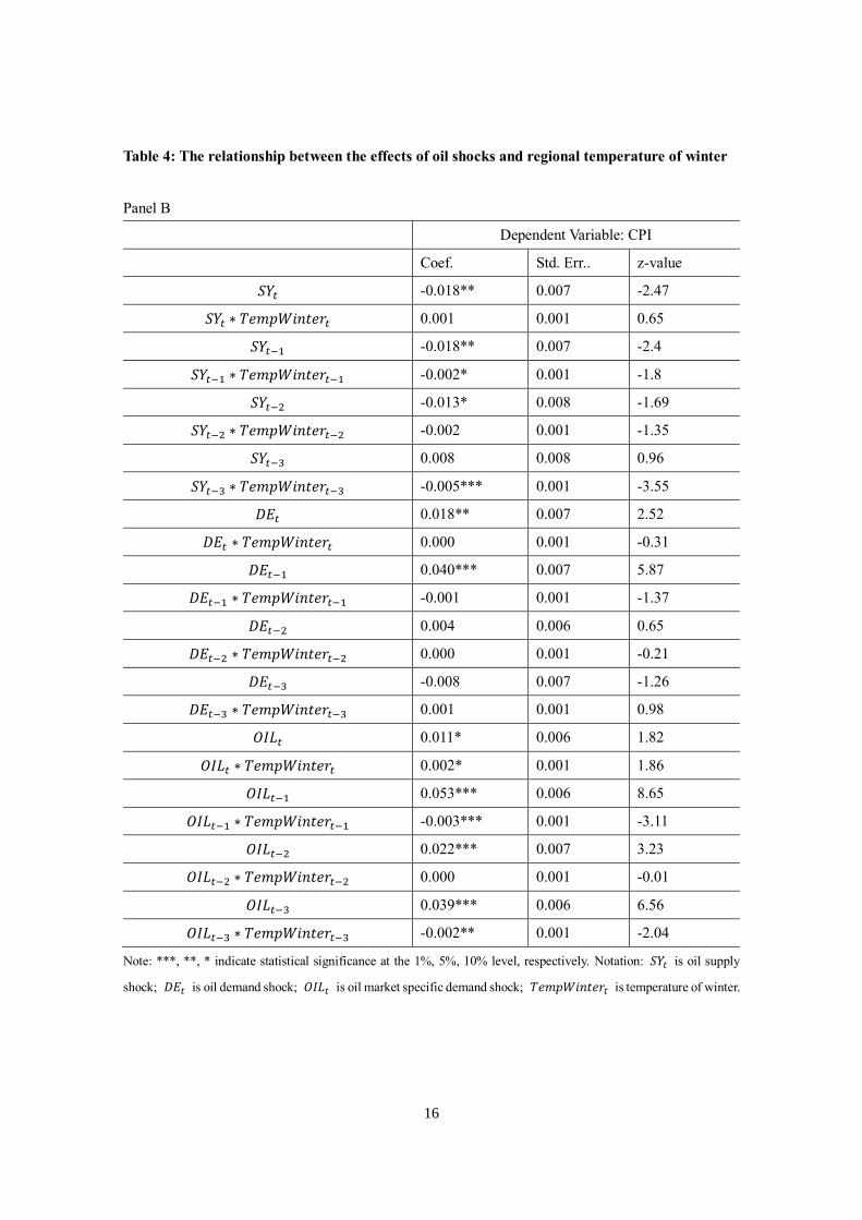
Table 4 shows the results for temperature of winter (𝑇𝑒𝑚𝑝𝑊𝑖𝑛𝑡𝑒𝑟𝑡 ). In Panel A, the

coefficient of the interaction term of 𝑂𝐼𝐿𝑡 and 𝑇𝑒𝑚𝑝𝑊𝑖𝑛𝑡𝑒𝑟𝑡 takes on a significantly negative

7

value at three lags, implying that, ceteris paribus, regions with lower temperatures during winter will

have output to be more negatively affected by oil price surges resulted from oil market specific demand

shocks. In Japan, regions with colder winter (i.e. those located the north or northeast of Japan, such as

Hokkaido, Aomori, Iwate and so on) consume more oil for heating and snowplowing during winter.

For this reason, an oil market specific demand shock, which raises the price of oil, may push up

production costs more in these regions than in those with warmer winter. In Panel B of Table 4, the

coefficients of the interaction terms of 𝑆𝑌𝑡 and 𝑇𝑒𝑚𝑝𝑊𝑖𝑛𝑡𝑒𝑟𝑡 at the one and three lags, as well as

those on the interaction terms of 𝑂𝐼𝐿𝑡 and 𝑇𝑒𝑚𝑝𝑊𝑖𝑛𝑡𝑒𝑟𝑡 at the two and three lags are significantly

negative. These imply that a region with colder winter will have the price level to be more affected by

oil supply shocks and oil market specific demand shocks. Our interpretation for this is the same as that

for result on output noted right above.

5. Concluding remarks

In this paper we address the question of how the effects of oil shocks on different economies

are affected by their heterogeneity. We take up the Japanese regional economies as a case study and

use a structural VAR model and a panel VAR model as the analytical framework.

Our main conclusion is that the effects of oil price shocks on the Japanese regional

economies are closely related to various natural and socio-economic characteristics of those regions.

More specifically, in the presence of a surge in the oil price caused by an oil demand shock originated

from the global real economic activity or an oil market specific demand shock, output is more

negatively affected and the price level rises more in a region with colder winter, or with lower

population density, or with a higher share of petroleum and coal products in total value added. In

addition, the effects of oil shocks also depend on the share in total value added of transport equipment

industry, one of the key industries of Japan: The more a region is specializing in this industry the more

its output and the less its price level respond to oil demand shocks. Interestingly, the last result, though

appears counterintuitive, can be explained based on the relationships between this the share of industry

and the general level of development of industries in a region, the dependency on goods imported from

other regions and transportation costs.

References

Arellano, Manuel and Olympia Bover, 1995, “Another look at the instrumental variable estimation of

error-components model,” Journal of Econometrics 68:1, 29-51.

Fukunaga, Ichiro, Naohisa Hirakata and Nao Sugo, 2009, “The Effects of Oil Price Changes on the

Industry-Level Production and Prices in the U.S. and Japan,” IMES Discussion Paper Series 09-

8

E-23, Institute for Monetary and Economic Studies, Bank of Japan

Iwaisako, Tokuo and Hayato Nakata, 2017. “Impact of exchange rate shocks on Japanese exports:

Quantitative assessment using a structural VAR model,” Journal of the Japanese and International

Economies 46:1, 1-16

Peersman, Gert and Ine Van Robays, 2009. “Oil and the Euro Area Economy.” Economic Policy

October 2009, 603–651.

Vu, Tuan Khai and Hayato Nakata, 2016. “Oil and the regional economies in Japan: Analysis using a

VAR with block exogeneity,” Paper presented at the WEAI 91th Annual Conference (Portland).

Vu, Tuan Khai and Hayato Nakata, 2018. “Oil price fluctuations and the small open economies of

Southeast Asia: An analysis using vector autoregression with block exogeneity,” Journal of Asian

Economics 54:1, 1-21

9

Table 1: The relationship between the effects of oil shocks and regional share of transportation

equipment in total value added

Panel A

Dependent Variable: IIP

Coef. Std. Err.. z-value

𝑆𝑌𝑡 0.036 0.035 1.01

𝑆𝑌𝑡 ∗ 𝑆ℎ𝑎𝑟𝑒𝑇𝑟𝑎𝑛𝑠𝑡 0.664* 0.385 1.72

𝑆𝑌𝑡−1 0.139*** 0.033 4.15

𝑆𝑌𝑡−1 ∗ 𝑆ℎ𝑎𝑟𝑒𝑇𝑟𝑎𝑛𝑠𝑡−1 0.131 0.360 0.36

𝑆𝑌𝑡−2 0.016 0.035 0.46

𝑆𝑌𝑡−2 ∗ 𝑆ℎ𝑎𝑟𝑒𝑇𝑟𝑎𝑛𝑠𝑡−2 -0.154 0.388 -0.4

𝑆𝑌𝑡−3 0.044 0.034 1.29

𝑆𝑌𝑡−3 ∗ 𝑆ℎ𝑎𝑟𝑒𝑇𝑟𝑎𝑛𝑠𝑡−3 -0.130 0.369 -0.35

𝐷𝐸𝑡 0.123** 0.047 2.61

𝐷𝐸𝑡 ∗ 𝑆ℎ𝑎𝑟𝑒𝑇𝑟𝑎𝑛𝑠𝑡 -0.315 0.444 -0.71

𝐷𝐸𝑡−1 0.042 0.045 0.94

𝐷𝐸𝑡−1 ∗ 𝑆ℎ𝑎𝑟𝑒𝑇𝑟𝑎𝑛𝑠𝑡−1 0.880** 0.393 2.24

𝐷𝐸𝑡−2 0.174*** 0.050 3.46

𝐷𝐸𝑡−2 ∗ 𝑆ℎ𝑎𝑟𝑒𝑇𝑟𝑎𝑛𝑠𝑡−2 1.001** 0.441 2.27

𝐷𝐸𝑡−3 0.217*** 0.050 4.35

𝐷𝐸𝑡−3 ∗ 𝑆ℎ𝑎𝑟𝑒𝑇𝑟𝑎𝑛𝑠𝑡−3 1.810*** 0.482 3.75

𝑂𝐼𝐿𝑡 0.150*** 0.042 3.61

𝑂𝐼𝐿𝑡 ∗ 𝑆ℎ𝑎𝑟𝑒𝑇𝑟𝑎𝑛𝑠𝑡 -0.314 0.456 -0.69

𝑂𝐼𝐿𝑡−1 0.148*** 0.040 3.74

𝑂𝐼𝐿𝑡−1 ∗ 𝑆ℎ𝑎𝑟𝑒𝑇𝑟𝑎𝑛𝑠𝑡−1 0.509 0.422 1.21

𝑂𝐼𝐿𝑡−2 0.143*** 0.042 3.42

𝑂𝐼𝐿𝑡−2 ∗ 𝑆ℎ𝑎𝑟𝑒𝑇𝑟𝑎𝑛𝑠𝑡−2 1.015** 0.461 2.2

𝑂𝐼𝐿𝑡−3 0.113*** 0.041 2.78

𝑂𝐼𝐿𝑡−3 ∗ 𝑆ℎ𝑎𝑟𝑒𝑇𝑟𝑎𝑛𝑠𝑡−3 0.898** 0.444 2.02

Note: ***, **, * indicate statistical significance at the 1%, 5%, 10% level, respectively. Notation: 𝑆𝑌𝑡 is oil supply

shock; 𝐷𝐸𝑡 is oil demand shock; 𝑂𝐼𝐿𝑡 is oil market specific demand shock; 𝑆ℎ𝑎𝑟𝑒𝑇𝑟𝑎𝑛𝑠𝑡 is share of transportation

equipment industry in total value added.

10

Table 1: The relationship between the effects of oil shocks and regional share of transportation

equipment in total value added

Panel B

Dependent Variable: CPI


𝑆𝑌𝑡 -0.016*** 0.005 -2.95

𝑆𝑌𝑡 ∗ 𝑆ℎ𝑎𝑟𝑒𝑇𝑟𝑎𝑛𝑠𝑡 0.026 0.047 0.55

𝑆𝑌𝑡−1 -0.031*** 0.005 -5.88

𝑆𝑌𝑡−1 ∗ 𝑆ℎ𝑎𝑟𝑒𝑇𝑟𝑎𝑛𝑠𝑡−1 0.040 0.047 0.85

𝑆𝑌𝑡−2 -0.021*** 0.005 -3.91

𝑆𝑌𝑡−2 ∗ 𝑆ℎ𝑎𝑟𝑒𝑇𝑟𝑎𝑛𝑠𝑡−2 0.002 0.048 0.04

𝑆𝑌𝑡−3 -0.015** 0.006 -2.49

𝑆𝑌𝑡−3 ∗ 𝑆ℎ𝑎𝑟𝑒𝑇𝑟𝑎𝑛𝑠𝑡−3 -0.024 0.050 -0.48

𝐷𝐸𝑡 0.022** 0.005 4.6

𝐷𝐸𝑡 ∗ 𝑆ℎ𝑎𝑟𝑒𝑇𝑟𝑎𝑛𝑠𝑡 -0.067 0.034 -1.96

𝐷𝐸𝑡−1 0.039** 0.005 8.06

𝐷𝐸𝑡−1 ∗ 𝑆ℎ𝑎𝑟𝑒𝑇𝑟𝑎𝑛𝑠𝑡−1 -0.066** 0.033 -1.99

𝐷𝐸𝑡−2 -0.002 0.004 -0.51

𝐷𝐸𝑡−2 ∗ 𝑆ℎ𝑎𝑟𝑒𝑇𝑟𝑎𝑛𝑠𝑡−2 0.055* 0.030 1.81

𝐷𝐸𝑡−3 -0.002 0.005 -0.33

𝐷𝐸𝑡−3 ∗ 𝑆ℎ𝑎𝑟𝑒𝑇𝑟𝑎𝑛𝑠𝑡−3 -0.014 0.032 -0.45

𝑂𝐼𝐿𝑡 0.018*** 0.004 4.15

𝑂𝐼𝐿𝑡 ∗ 𝑆ℎ𝑎𝑟𝑒𝑇𝑟𝑎𝑛𝑠𝑡 0.042 0.033 1.25

𝑂𝐼𝐿𝑡−1 0.039*** 0.004 9.22

𝑂𝐼𝐿𝑡−1 ∗ 𝑆ℎ𝑎𝑟𝑒𝑇𝑟𝑎𝑛𝑠𝑡−1 -0.027 0.033 -0.81

𝑂𝐼𝐿𝑡−2 0.021*** 0.005 4.46


𝑂𝐼𝐿𝑡−3 0.026*** 0.004 6.26



shock; 𝐷𝐸𝑡 is oil demand shock; 𝑂𝐼𝐿𝑡 is oil market specific demand shock; 𝑆ℎ𝑎𝑟𝑒𝑇𝑟𝑎𝑛𝑠𝑡 is share of transportation

equipment industry in total value added.

11

Table 2: The relationship between the effects of oil shocks and regional share of petroleum and

coal products in total value added

Panel A



𝑆𝑌𝑡 0.090*** 0.028 3.18

𝑆𝑌𝑡 ∗ 𝑆ℎ𝑎𝑟𝑒𝑃𝑒𝑡𝑟𝑜𝐶𝑜𝑎𝑙𝑡 -0.573 0.907 -0.63

𝑆𝑌𝑡−1 0.136*** 0.028 4.84

𝑆𝑌𝑡−1 ∗ 𝑆ℎ𝑎𝑟𝑒𝑃𝑒𝑡𝑟𝑜𝐶𝑜𝑎𝑙𝑡−1 0.207 0.916 0.23

𝑆𝑌𝑡−2 0.009 0.030 0.32


𝑆𝑌𝑡−3 0.043 0.028 1.55

𝑆𝑌𝑡−3 ∗ 𝑆ℎ𝑎𝑟𝑒𝑃𝑒𝑡𝑟𝑜𝐶𝑜𝑎𝑙𝑡−3 -0.377 1.055 -0.36

𝐷𝐸𝑡 0.102*** 0.039 2.63

𝐷𝐸𝑡 ∗ 𝑆ℎ𝑎𝑟𝑒𝑃𝑒𝑡𝑟𝑜𝐶𝑜𝑎𝑙𝑡 1.110 1.296 0.86

𝐷𝐸𝑡−1 0.136*** 0.038 3.58

𝐷𝐸𝑡−1 ∗ 𝑆ℎ𝑎𝑟𝑒𝑃𝑒𝑡𝑟𝑜𝐶𝑜𝑎𝑙𝑡−1 0.189 1.333 0.14

𝐷𝐸𝑡−2 0.246*** 0.043 5.74

𝐷𝐸𝑡−2 ∗ 𝑆ℎ𝑎𝑟𝑒𝑃𝑒𝑡𝑟𝑜𝐶𝑜𝑎𝑙𝑡−2 -0.621 1.633 -0.38

𝐷𝐸𝑡−3 0.357*** 0.040 8.96


𝑂𝐼𝐿𝑡 0.134*** 0.034 3.95

𝑂𝐼𝐿𝑡 ∗ 𝑆ℎ𝑎𝑟𝑒𝑃𝑒𝑡𝑟𝑜𝐶𝑜𝑎𝑙𝑡 -0.993 1.338 -0.74

𝑂𝐼𝐿𝑡−1 0.210*** 0.032 6.48

𝑂𝐼𝐿𝑡−1 ∗ 𝑆ℎ𝑎𝑟𝑒𝑃𝑒𝑡𝑟𝑜𝐶𝑜𝑎𝑙𝑡−1 -2.235* 1.238 -1.8

𝑂𝐼𝐿𝑡−2 0.215*** 0.032 6.66

𝑂𝐼𝐿𝑡−2 ∗ 𝑆ℎ𝑎𝑟𝑒𝑃𝑒𝑡𝑟𝑜𝐶𝑜𝑎𝑙𝑡−2 -0.631 1.360 -0.46

𝑂𝐼𝐿𝑡−3 0.196*** 0.033 5.97

𝑂𝐼𝐿𝑡−3 ∗ 𝑆ℎ𝑎𝑟𝑒𝑃𝑒𝑡𝑟𝑜𝐶𝑜𝑎𝑙𝑡−3 -2.574*** 1.464 -1.76


shock; 𝐷𝐸𝑡 is oil demand shock; 𝑂𝐼𝐿𝑡 is oil market specific demand shock; 𝑆ℎ𝑎𝑟𝑒𝑃𝑒𝑡𝑟𝑜𝐶𝑜𝑎𝑙𝑡 is share of

petroleum and coal products industry in total value added.

12

Table 2: The relationship between the effects of oil shocks and regional share of petroleum and

coal products in total value added

Panel B



𝑆𝑌𝑡 -0.015*** 0.005 -3.27

𝑆𝑌𝑡 ∗ 𝑆ℎ𝑎𝑟𝑒𝑃𝑒𝑡𝑟𝑜𝐶𝑜𝑎𝑙𝑡 0.049 0.180 0.27

𝑆𝑌𝑡−1 -0.025*** 0.004 -5.72

𝑆𝑌𝑡−1 ∗ 𝑆ℎ𝑎𝑟𝑒𝑃𝑒𝑡𝑟𝑜𝐶𝑜𝑎𝑙𝑡−1 -0.383** 0.154 -2.49

𝑆𝑌𝑡−2 -0.022*** 0.004 -4.97


𝑆𝑌𝑡−3 -0.019*** 0.005 -3.81


𝐷𝐸𝑡 0.012*** 0.004 2.86

𝐷𝐸𝑡 ∗ 𝑆ℎ𝑎𝑟𝑒𝑃𝑒𝑡𝑟𝑜𝐶𝑜𝑎𝑙𝑡 0.506*** 0.172 2.94

𝐷𝐸𝑡−1 0.031*** 0.004 7.8

𝐷𝐸𝑡−1 ∗ 𝑆ℎ𝑎𝑟𝑒𝑃𝑒𝑡𝑟𝑜𝐶𝑜𝑎𝑙𝑡−1 0.209 0.175 1.19

𝐷𝐸𝑡−2 0.004 0.004 1.03

𝐷𝐸𝑡−2 ∗ 𝑆ℎ𝑎𝑟𝑒𝑃𝑒𝑡𝑟𝑜𝐶𝑜𝑎𝑙𝑡−2 -0.353** 0.175 -2.01

𝐷𝐸𝑡−3 -0.002 0.004 -0.54


𝑂𝐼𝐿𝑡 0.017*** 0.004 4.62

𝑂𝐼𝐿𝑡 ∗ 𝑆ℎ𝑎𝑟𝑒𝑃𝑒𝑡𝑟𝑜𝐶𝑜𝑎𝑙𝑡 0.205 0.174 1.18

𝑂𝐼𝐿𝑡−1 0.037*** 0.004 10.56


𝑂𝐼𝐿𝑡−2 0.017*** 0.004 4.31

𝑂𝐼𝐿𝑡−2 ∗ 𝑆ℎ𝑎𝑟𝑒𝑃𝑒𝑡𝑟𝑜𝐶𝑜𝑎𝑙𝑡−2 0.172 0.177 0.97

𝑂𝐼𝐿𝑡−3 0.029*** 0.004 8.32



shock; 𝐷𝐸𝑡 is oil demand shock; 𝑂𝐼𝐿𝑡 is oil market specific demand shock; 𝑆ℎ𝑎𝑟𝑒𝑃𝑒𝑡𝑟𝑜𝐶𝑜𝑎𝑙𝑡 is share of

petroleum and coal products industry in total value added.

13

Table 3: The relationship between the effects of oil shocks and regional population density

Panel A



𝑆𝑌𝑡 0.095*** 0.029 3.23

𝑆𝑌𝑡 ∗ 𝑃𝐷𝑡 -0.019 0.020 -0.94

𝑆𝑌𝑡−1 0.135*** 0.027 4.96

𝑆𝑌𝑡−1 ∗ 𝑃𝐷𝑡−1 0.022 0.019 1.15

𝑆𝑌𝑡−2 0.005 0.029 0.18

𝑆𝑌𝑡−2 ∗ 𝑃𝐷𝑡−2 -0.001 0.021 -0.03

𝑆𝑌𝑡−3 0.050* 0.028 1.8

𝑆𝑌𝑡−3 ∗ 𝑃𝐷𝑡−3 -0.025 0.019 -1.36

𝐷𝐸𝑡 0.087** 0.037 2.33

𝐷𝐸𝑡 ∗ 𝑃𝐷𝑡 0.008 0.020 0.4

𝐷𝐸𝑡−1 0.113*** 0.037 3.1

𝐷𝐸𝑡−1 ∗ 𝑃𝐷𝑡−1 0.012 0.022 0.52

𝐷𝐸𝑡−2 0.273*** 0.042 6.55

𝐷𝐸𝑡−2 ∗ 𝑃𝐷𝑡−2 -0.011 0.024 -0.44

𝐷𝐸𝑡−3 0.387*** 0.038 10.29

𝐷𝐸𝑡−3 ∗ 𝑃𝐷𝑡−3 -0.005 0.023 -0.22

𝑂𝐼𝐿𝑡 0.133*** 0.034 3.92

𝑂𝐼𝐿𝑡 ∗ 𝑃𝐷𝑡 -0.013 0.021 -0.61

𝑂𝐼𝐿𝑡−1 0.183*** 0.032 5.67

𝑂𝐼𝐿𝑡−1 ∗ 𝑃𝐷𝑡−1 0.010 0.021 0.5

𝑂𝐼𝐿𝑡−2 0.224*** 0.031 7.13

𝑂𝐼𝐿𝑡−2 ∗ 𝑃𝐷𝑡−2 -0.002 0.021 -0.12

𝑂𝐼𝐿𝑡−3 0.198*** 0.032 6.18

𝑂𝐼𝐿𝑡−3 ∗ 𝑃𝐷𝑡−3 -0.018 0.021 -0.87


shock; 𝐷𝐸𝑡 is oil demand shock; 𝑂𝐼𝐿𝑡 is oil market specific demand shock; 𝑃𝐷𝑡 is population density.

14

Table 3: The relationship between the effects of oil shocks and regional population density

Panel B



𝑆𝑌𝑡 -0.014*** 0.004 -3.08

𝑆𝑌𝑡 ∗ 𝑃𝐷𝑡 -0.001 0.003 -0.19

𝑆𝑌𝑡−1 -0.030*** 0.004 -6.73

𝑆𝑌𝑡−1 ∗ 𝑃𝐷𝑡−1 0.002 0.003 0.66

𝑆𝑌𝑡−2 -0.021*** 0.005 -4.72

𝑆𝑌𝑡−2 ∗ 𝑃𝐷𝑡−2 0.000 0.003 0.05

𝑆𝑌𝑡−3 -0.015*** 0.005 -3.06

𝑆𝑌𝑡−3 ∗ 𝑃𝐷𝑡−3 -0.002 0.003 -0.69

𝐷𝐸𝑡 0.018*** 0.004 4.51

𝐷𝐸𝑡 ∗ 𝑃𝐷𝑡 -0.002 0.002 -1.02

𝐷𝐸𝑡−1 0.035*** 0.004 9.39

𝐷𝐸𝑡−1 ∗ 𝑃𝐷𝑡−1 -0.004** 0.002 -1.98

𝐷𝐸𝑡−2 0.005 0.003 1.38

𝐷𝐸𝑡−2 ∗ 𝑃𝐷𝑡−2 -0.003 0.002 -1.39

𝐷𝐸𝑡−3 -0.003 0.004 -0.69

𝐷𝐸𝑡−3 ∗ 𝑃𝐷𝑡−3 -0.001 0.002 -0.24

𝑂𝐼𝐿𝑡 0.022*** 0.004 6.2

𝑂𝐼𝐿𝑡 ∗ 𝑃𝐷𝑡 -0.001 0.002 -0.39

𝑂𝐼𝐿𝑡−1 0.041*** 0.003 11.92

𝑂𝐼𝐿𝑡−1 ∗ 𝑃𝐷𝑡−1 -0.006*** 0.002 -3.12

𝑂𝐼𝐿𝑡−2 0.024*** 0.004 6.11

𝑂𝐼𝐿𝑡−2 ∗ 𝑃𝐷𝑡−2 -0.003 0.002 -1.13

𝑂𝐼𝐿𝑡−3 0.030*** 0.003 8.81

𝑂𝐼𝐿𝑡−3 ∗ 𝑃𝐷𝑡−3 -0.001 0.002 -0.74


shock; 𝐷𝐸𝑡 is oil demand shock; 𝑂𝐼𝐿𝑡 is oil market specific demand shock; 𝑃𝐷𝑡 is population density.

15

Table 4: The relationship between the effects of oil shocks and regional temperature of winter

Panel A



𝑆𝑌𝑡 0.129*** 0.049 2.64

𝑆𝑌𝑡 ∗ 𝑇𝑒𝑚𝑝𝑊𝑖𝑛𝑡𝑒𝑟𝑡 -0.009 0.009 -1.02

𝑆𝑌𝑡−1 0.128*** 0.048 2.69

𝑆𝑌𝑡−1 ∗ 𝑇𝑒𝑚𝑝𝑊𝑖𝑛𝑡𝑒𝑟𝑡−1 0.004 0.008 0.46

𝑆𝑌𝑡−2 0.055 0.052 1.07

𝑆𝑌𝑡−2 ∗ 𝑇𝑒𝑚𝑝𝑊𝑖𝑛𝑡𝑒𝑟𝑡−2 -0.010 0.009 -1.08

𝑆𝑌𝑡−3 0.018 0.049 0.37

𝑆𝑌𝑡−3 ∗ 𝑇𝑒𝑚𝑝𝑊𝑖𝑛𝑡𝑒𝑟𝑡−3 0.003 0.009 0.34

𝐷𝐸𝑡 0.082 0.065 1.27

𝐷𝐸𝑡 ∗ 𝑇𝑒𝑚𝑝𝑊𝑖𝑛𝑡𝑒𝑟𝑡 0.002 0.011 0.17

𝐷𝐸𝑡−1 0.162*** 0.061 2.67

𝐷𝐸𝑡−1 ∗ 𝑇𝑒𝑚𝑝𝑊𝑖𝑛𝑡𝑒𝑟𝑡−1 -0.008 0.010 -0.78

𝐷𝐸𝑡−2 0.373*** 0.075 4.98

𝐷𝐸𝑡−2 ∗ 𝑇𝑒𝑚𝑝𝑊𝑖𝑛𝑡𝑒𝑟𝑡−2 -0.020 0.013 -1.59

𝐷𝐸𝑡−3 0.369*** 0.064 5.77

𝐷𝐸𝑡−3 ∗ 𝑇𝑒𝑚𝑝𝑊𝑖𝑛𝑡𝑒𝑟𝑡−3 0.003 0.011 0.24

𝑂𝐼𝐿𝑡 0.071 0.062 1.14

𝑂𝐼𝐿𝑡 ∗ 𝑇𝑒𝑚𝑝𝑊𝑖𝑛𝑡𝑒𝑟𝑡 0.010 0.010 0.97

𝑂𝐼𝐿𝑡−1 0.151*** 0.054 2.79

𝑂𝐼𝐿𝑡−1 ∗ 𝑇𝑒𝑚𝑝𝑊𝑖𝑛𝑡𝑒𝑟𝑡−1 0.007 0.009 0.78

𝑂𝐼𝐿𝑡−2 0.247*** 0.056 4.42

𝑂𝐼𝐿𝑡−2 ∗ 𝑇𝑒𝑚𝑝𝑊𝑖𝑛𝑡𝑒𝑟𝑡−2 -0.005 0.010 -0.46

𝑂𝐼𝐿𝑡−3 0.306*** 0.055 5.52

𝑂𝐼𝐿𝑡−3 ∗ 𝑇𝑒𝑚𝑝𝑊𝑖𝑛𝑡𝑒𝑟𝑡−3 -0.023** 0.009 -2.43


shock; 𝐷𝐸𝑡 is oil demand shock; 𝑂𝐼𝐿𝑡 is oil market specific demand shock; 𝑇𝑒𝑚𝑝𝑊𝑖𝑛𝑡𝑒𝑟𝑡 is temperature of winter.

16

Table 4: The relationship between the effects of oil shocks and regional temperature of winter

Panel B



𝑆𝑌𝑡 -0.018** 0.007 -2.47

𝑆𝑌𝑡 ∗ 𝑇𝑒𝑚𝑝𝑊𝑖𝑛𝑡𝑒𝑟𝑡 0.001 0.001 0.65

𝑆𝑌𝑡−1 -0.018** 0.007 -2.4

𝑆𝑌𝑡−1 ∗ 𝑇𝑒𝑚𝑝𝑊𝑖𝑛𝑡𝑒𝑟𝑡−1 -0.002* 0.001 -1.8

𝑆𝑌𝑡−2 -0.013* 0.008 -1.69

𝑆𝑌𝑡−2 ∗ 𝑇𝑒𝑚𝑝𝑊𝑖𝑛𝑡𝑒𝑟𝑡−2 -0.002 0.001 -1.35

𝑆𝑌𝑡−3 0.008 0.008 0.96

𝑆𝑌𝑡−3 ∗ 𝑇𝑒𝑚𝑝𝑊𝑖𝑛𝑡𝑒𝑟𝑡−3 -0.005*** 0.001 -3.55

𝐷𝐸𝑡 0.018** 0.007 2.52

𝐷𝐸𝑡 ∗ 𝑇𝑒𝑚𝑝𝑊𝑖𝑛𝑡𝑒𝑟𝑡 0.000 0.001 -0.31

𝐷𝐸𝑡−1 0.040*** 0.007 5.87

𝐷𝐸𝑡−1 ∗ 𝑇𝑒𝑚𝑝𝑊𝑖𝑛𝑡𝑒𝑟𝑡−1 -0.001 0.001 -1.37

𝐷𝐸𝑡−2 0.004 0.006 0.65

𝐷𝐸𝑡−2 ∗ 𝑇𝑒𝑚𝑝𝑊𝑖𝑛𝑡𝑒𝑟𝑡−2 0.000 0.001 -0.21

𝐷𝐸𝑡−3 -0.008 0.007 -1.26

𝐷𝐸𝑡−3 ∗ 𝑇𝑒𝑚𝑝𝑊𝑖𝑛𝑡𝑒𝑟𝑡−3 0.001 0.001 0.98

𝑂𝐼𝐿𝑡 0.011* 0.006 1.82

𝑂𝐼𝐿𝑡 ∗ 𝑇𝑒𝑚𝑝𝑊𝑖𝑛𝑡𝑒𝑟𝑡 0.002* 0.001 1.86

𝑂𝐼𝐿𝑡−1 0.053*** 0.006 8.65

𝑂𝐼𝐿𝑡−1 ∗ 𝑇𝑒𝑚𝑝𝑊𝑖𝑛𝑡𝑒𝑟𝑡−1 -0.003*** 0.001 -3.11

𝑂𝐼𝐿𝑡−2 0.022*** 0.007 3.23

𝑂𝐼𝐿𝑡−2 ∗ 𝑇𝑒𝑚𝑝𝑊𝑖𝑛𝑡𝑒𝑟𝑡−2 0.000 0.001 -0.01

𝑂𝐼𝐿𝑡−3 0.039*** 0.006 6.56

𝑂𝐼𝐿𝑡−3 ∗ 𝑇𝑒𝑚𝑝𝑊𝑖𝑛𝑡𝑒𝑟𝑡−3 -0.002** 0.001 -2.04


shock; 𝐷𝐸𝑡 is oil demand shock; 𝑂𝐼𝐿𝑡 is oil market specific demand shock; 𝑇𝑒𝑚𝑝𝑊𝑖𝑛𝑡𝑒𝑟𝑡 is temperature of winter.

oil shocks and regional heterogeneity: the case of japan · legislation in euro area countries. vu...

Documents