The Desktop GIS OpenJUMP: A hands-on introduction

OGRS 2009 Workshop

Stefan Steiniger and Michaël Michaud

This tutorial is based on original material by E. Bocher and A. Lepetit prepared for the FOSS4G 2006 conference in Lausanne.

1/32

Table of contents

Introduction page 3

I - Using OpenJUMP page 5

1. Loading and displaying data page 52. Working with alphanumeric data page 93. Thematic maps page 144. Exporting views page 165. Printing page 176. Querying data page 207. Geometric data creation and editing page 24

II - Using OpenJUMP with PostGIS page 26

1. OpenJUMP and PostGIS page 261.1 Creating a database page 261.2 Loading the PostGIS extension page 271.3 Using PostGIS page 28

1.3.1 Populating the database page 281.3.2 Loading data from the database page 291.3.3 Performing SQL queries page 30

2/32

Introduction

Summary

The aim of the workshop is to introduce the Free GIS software OpenJUMP and to show how OpenJUMP can be used to visualise, create, edit and analyse geographic data. With those capabilities OpenJUMP is a full functional Desktop GIS that can be used in several places of a Spatial Data Infrastructure (SDI). Figure 1 illustrates the use of Desktop GIS in a SDI context.

This document is organised in two parts which allow a progressive learning of OpenJUMP.

1. Using OpenJUMPThe first part guides you through some basic OpenJUMP skills. You will learn how to :

– load and display data,– work with alphanumeric data,– create thematic maps,– export views– print– query and analyse data– create and edit geometry data

2. Using OpenJUMP with PostGIS

This part is probably not presented in the workshop but is additionally provided for the interested user. This part will demonstrate how it's possible to write, access and query data stored in the PostGIS database. You will learn how to:

– store data to PostGIS– read data from PostGIS– query the data with spatial and numeric predicates,– build expressions with more than one criteria

3/32

Figure 1 - Using OpenJUMP in a Spatial Data Infrastructure (SDI)

Requirements

You should know the basic GIS concepts, e.g. you should know the difference between raster and vector data, should know basic analysis functions such as buffering and overlay (intersection) operations, and you should know the principles of cartographic representation and classification.

Working fully through the tutorial will require about 2 hours (trained users will need 70 mins for part 1 and 10 mins for part 2) .

Materials

We need : • OpenJUMP 1.3 available on http://www.openjump.org,

• The following OpenJUMP plugins (extensions) installed:

• CadPlan's JumpPrinter extension (http://www.cadplan.com.au/)

• PostGIS plugin (http://sourceforge.net/project/showfiles.php?group_id=118054)

• PostgreSQL 6.3 database (the PostGIS extension and pgAdmin should be included in the PostgreSQL distribution) available at http://www.postgresql.org/ and http://postgis.refractions.net

• OpenOffice 3.x available at http://www.openoffice.org/,

And the spatial data delivered with this tutorial (see the table below).

Data

Data Geometry Description

frenchprovinces polygon Regional country

departement22 polygon French sub country after province

municipalities22 polygon Municipalities for Côtes-d'Armor departement

watershed polygon Watershed name's Sterenn

subwaterhed polygon Sub watershed in Sterenn

wsmunicipalities polygon Municipalities crossing Sterenn watershed

waternetwork line Ditches and rivers in Sterenn watershed

landcover2000 polygon Land cover classification in 2000

hedgerow line Hedges network in Sterenn watershed

F018_024.TIF

F018_025.TIF

photo2.ecw

photo3.ecw

Raster images

Topographic map (tif + world file)

Topographic map (tif + world file)

Aerial photography (ecw)

pop22-5499.ods --- Population by municipality 1954 to 1999 in Côtes-d'Armor (Bretagne), Department 22

4/32

I - Using OpenJUMP

1 Loading and displaying data

1.1 Loading and organising data

When OpenJump starts, you see a main window named “project” (Figure 2). A “project” is not only a window which allows data visualisation and organisation but it’s a file too, which must contains all the work you do with OpenJump (.jmp extension).

First, you will load some vector data layers. So, from the Menu choose [File>Open...] click on “File” icon in the left sidebar and select:

• frenchprovinces.shp,• departement22.shp,• municipalities22.shp,

Another option to load vector data on Windows systems is to “drag & drop” files.

The layers that have been loaded are listed in a table of contents, to the left of the visualisation window (figure 3). We will call this window Layer View.

5/32

Figure 2 - OpenJUMP 1.3 workbench

Figure 3

There are several ways to move in the Layer View and to zoom into or out of the areas shown in it. Try out the use navigation tools that are provided in the toolbar, in the [View] menu, or by choosing a function from the mouse context menus accessible via a right-mouse-click on category name (e.g. “Working”) or layer name (e.g. municipalities22).

zoom in/out, or use the mouse wheel

pan map view

zoom to full extent or [View>Zoom To full Extend]

zoom to previous/next view

zoom to fence

zoom to selected items or [View>Zoom To Selected Items]

zoom to scale [View>Zoom to scale]

zoom to layer or layers layer context menu

1.2 Modifying layer properties

To modify the display of a layer you can use the Styles dialog (figure 4).

• The Rendering Tab (figure 5) enables you to change general properties (colour, transparency, line width and pattern, vertices visibility).

• The Scale Tab (figure 6) allows you to customise the display of a layer with respect to the zoom scale. So you can define that a layer can be shown only between a smallest and a largest scale. To obtain the current scale you can use [View>Show Scale].

• The Labels Tab (figure 7) enables you to define labelling options (font type, colour and height and placement options). Important is to know the attribute that contains the text to display.

6/32

Figure 4 - accessing the style dialog

Exercise 1 (figure 8)

Symbolise frenchprovinces- uncheck fill - change line colour to grey with width=7

Symbolise departement22- uncheck fill- make lines black with width=2

Symbolise municipalities22- Use from the preset styles the yellow one- Label using attribute “name_mun” check the box “Draw outline (halo)...”

7/32

Figure 7 - Labeling dialog

Figure 5 - Rendering dialog

Figure 6 - map visibility dialog

Figure 8 - customized display of our dataset

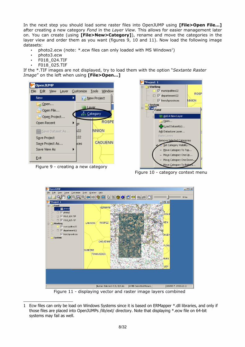
In the next step you should load some raster files into OpenJUMP using [File>Open File...] after creating a new category Fond in the Layer View. This allows for easier management later on. You can create (using [File>New>Category]), rename and move the categories in the layer view and order them as you want (figures 9, 10 and 11). Now load the following image datasets:

• photo2.ecw (note: *.ecw files can only loaded with MS Windows1)• photo3.ecw• F018_024.TIF• F018_025.TIF

If the *.TIF images are not displayed, try to load them with the option “Sextante Raster Image” on the left when using [File>Open...]

1 Ecw files can only be load on Windows Systems since it is based on ERMapper *.dll libraries, and only if those files are placed into OpenJUMPs /lib/ext/ directory. Note that displaying *.ecw file on 64-bit systems may fail as well.

8/32

Figure 11 - displaying vector and raster image layers combined

Figure 10 - category context menuFigure 9 - creating a new category

Exercise 2: customise the display of the raster image for certain zoom levels

• if you have OpenJUMP running on Windows load photo2.ecw and photo3.ecw - and set the smallest display scale to 12 000 (otherwise skip this step)

• for F018_024.TIF and F018_025.TIF, set smallest scale = 15 000 by using the Style dialogs accessible via the layer context mouse menu.

The current display scale can be turned on using [View>Show scale]

2 Working with alphanumeric data

2.1 Viewing attributes

In a layer, each feature has alphanumeric attributes. If you want to inspect the attributes of layer, then you can use the table icon from the toolbar or choose [View>Edit attributes] from the layer context menu (figure 12).

You will see a new window named “Attributes” (figure 14).

9/32

Figure 12 - accessing the attribute view / table view

Figure 13 - the attribute window

Another way to view attributes for a particular object is to use the Feature Info Tool from the toolbar:

2.2 Importing and joining alphanumeric data

In the next step we want to join demographic data stored in a table (from Excel or OpenOffice) with the polygons that describe the municipal areas, i.e. the dataset “municipalities22”.

Open the file pop22-5499.ods with OpenOffice. Go to [File>Save As...]. Choose the format Text CSV (.csv) from the drop down list, click “save”, click in the next dialog on “Keep Current Format”, and set the values in the following dialog as given in figure 14.

Now we go back to OpenJUMP and chose from the menu [Tools>Edit Attributes>Join TXT table...] (figure 15).

In the dialog that appears navigate to the folder where you stored the file pop22-5499.csv, chose from the file types drop down menu “All Files” and select the CSV file. In the next dialog chose the dataset/layer to which we like to append the fields, i.e. municipalities22.

In the following dialog we will need to select a unique key in both datasets that allows us to attach the information contained in the table data with the information in the geographic dataset. Set the values as shown in figure 16.

10/32

Figure 14 - exporting table data to *.csv format.

Figure 15

Figure 16 - Setting unique keys.

Afterwards the attributes of the table are appended to the layer's attribute table (figure 17).

To keep the result, you need to save the layer by choosing from the municipalities22 layer context menu (right mouse click on layer name) the function [Save Dataset As...].

2.3 Editing attributes of a layer

With OpenJUMP you can easily add or remove fields from a table data when the layer is editable. Right-click on the layer municipalities22 and check “Editable” (figure 18). If the layer is editable the layer name should be displayed yellow in the Layer View. You will also notice that a toolbox will appear that allows to edit the geometries in a layer.

11/32

Figure 18 - Making a layer editable

Figure 17

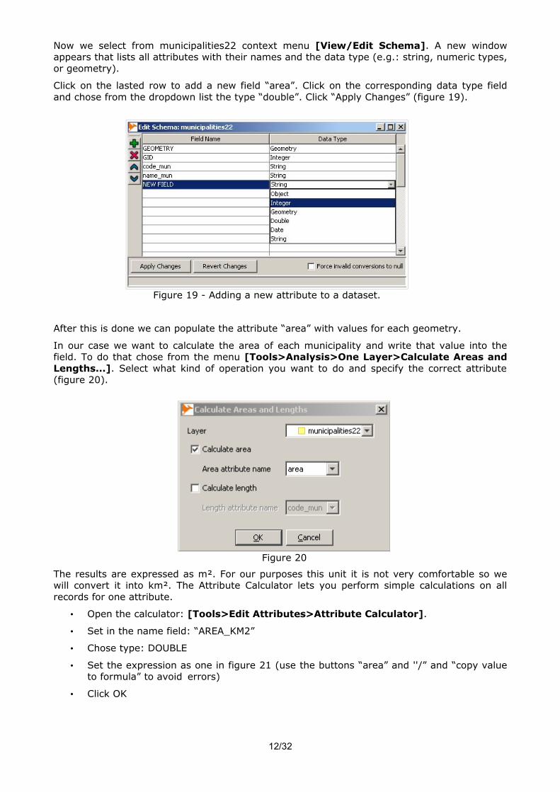
Now we select from municipalities22 context menu [View/Edit Schema]. A new window appears that lists all attributes with their names and the data type (e.g.: string, numeric types, or geometry).

Click on the lasted row to add a new field “area”. Click on the corresponding data type field and chose from the dropdown list the type “double”. Click “Apply Changes” (figure 19).

After this is done we can populate the attribute “area” with values for each geometry.

In our case we want to calculate the area of each municipality and write that value into the field. To do that chose from the menu [Tools>Analysis>One Layer>Calculate Areas and Lengths...]. Select what kind of operation you want to do and specify the correct attribute (figure 20).

The results are expressed as m². For our purposes this unit it is not very comfortable so we will convert it into km². The Attribute Calculator lets you perform simple calculations on all records for one attribute.

• Open the calculator: [Tools>Edit Attributes>Attribute Calculator].

• Set in the name field: “AREA_KM2”

• Chose type: DOUBLE

• Set the expression as one in figure 21 (use the buttons “area” and ''/” and “copy value to formula” to avoid errors)

• Click OK

12/32

Figure 19 - Adding a new attribute to a dataset.

Figure 20

This tool will create automatically the new field (area_km2) in the attribute table (figure 22).

13/32

Figure 21 - the attribute calculator

Figure 22 - The new field AREA_KM2 created with the calculator.

Exercise 3 (figure 23)

Calculate population densities for the years 1999 and 1954 for the layer municipalities22 using the Attribute Calculator.

The fields with the population counts are PMUN99 and PMUM54, respectively.

The population density is given as density_year = (population_count_year / km²)

3 Thematic maps

Here we want to create some thematic maps to display and compare the population density overtime that we just calculated in the previous section (2.3). Hence we will utilize OpenJUMP functions to do a classification of the density data and viewing tools to visually compare between the population density for the year 1954 and 1999.

• First, we create a new project [File>New>New Project].

• Select the layer municipalities22 in the original project and chose [Copy Selected Layers] from the layer context menu.

• Then go to the newly create project an chose [Paste Layers] from the category context menu for the category named “working”.

• Select [Window>Mosaic].

• Select [Window>Synchronisation>Synchronize pan and zoom] Now click in one Map View and zoom and pan. The views should be synchronized (figure 24).

14/32

Figure 23 - Result of Exercise 3, i.e. calculated population density

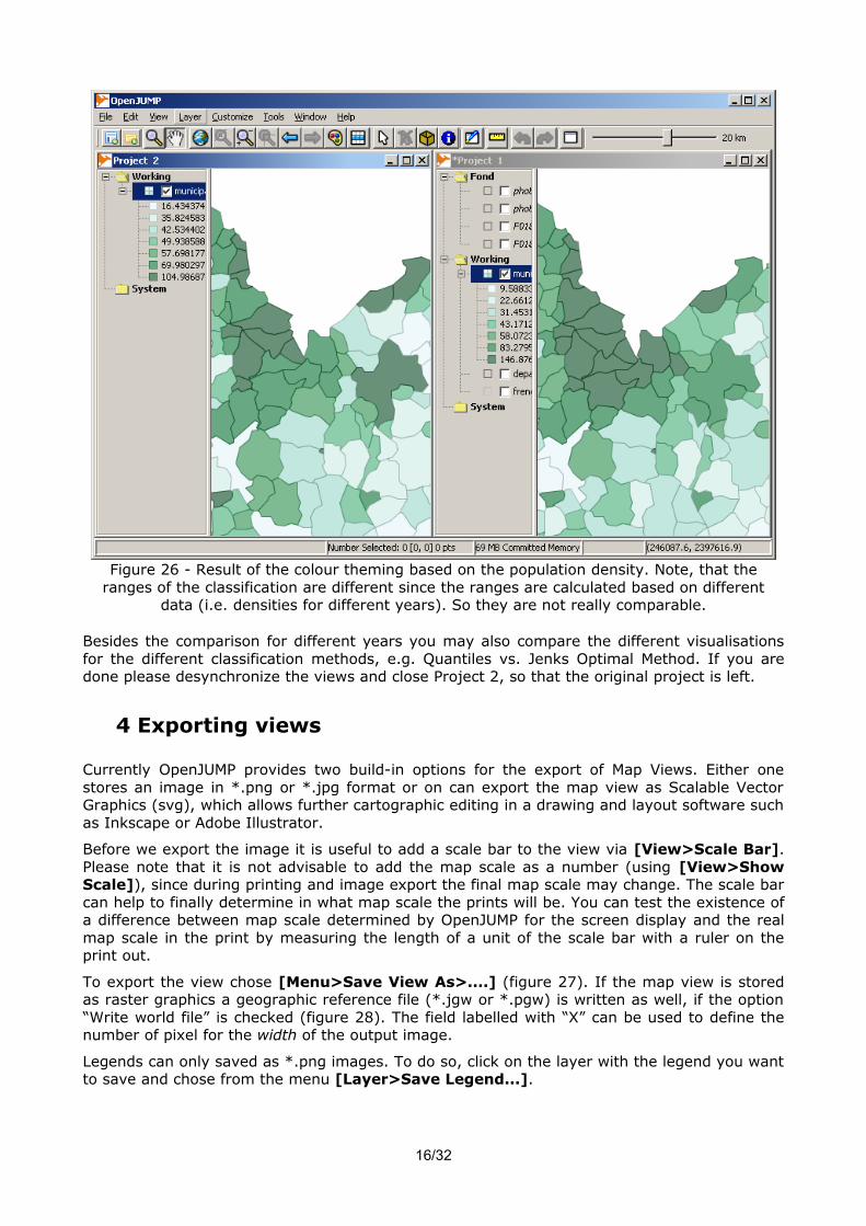
Now we use OpenJUMPs color theming functions from the Styling Dialog to display the population density in different colour scales layer (see figure 25 and 26). Open the “change styles” window (using the palette button). The Colour theming tab enables you to choose among several classification methods, the number of classes and the attribute that should be displayed in a colour. Apply the following colour theming (Quantile classification, 7 classes, green colour schema):

• project 1 : population density for 1954• project 2 : population density for 1999

Note: Please control that after changing the classification method the correct attribute field is chosen. Since values may be reset after the classification method is changed.

15/32

Figure 24 - Synchronising Map Views of different projects.

Figure 25 apply colour theming to the dataset (result in Figure 26)

Besides the comparison for different years you may also compare the different visualisations for the different classification methods, e.g. Quantiles vs. Jenks Optimal Method. If you are done please desynchronize the views and close Project 2, so that the original project is left.

4 Exporting views

Currently OpenJUMP provides two build-in options for the export of Map Views. Either one stores an image in *.png or *.jpg format or on can export the map view as Scalable Vector Graphics (svg), which allows further cartographic editing in a drawing and layout software such as Inkscape or Adobe Illustrator.

Before we export the image it is useful to add a scale bar to the view via [View>Scale Bar]. Please note that it is not advisable to add the map scale as a number (using [View>Show Scale]), since during printing and image export the final map scale may change. The scale bar can help to finally determine in what map scale the prints will be. You can test the existence of a difference between map scale determined by OpenJUMP for the screen display and the real map scale in the print by measuring the length of a unit of the scale bar with a ruler on the print out.

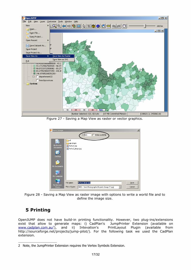
To export the view chose [Menu>Save View As>....] (figure 27). If the map view is stored as raster graphics a geographic reference file (*.jgw or *.pgw) is written as well, if the option “Write world file” is checked (figure 28). The field labelled with “X” can be used to define the number of pixel for the width of the output image.

Legends can only saved as *.png images. To do so, click on the layer with the legend you want to save and chose from the menu [Layer>Save Legend...].

16/32

Figure 26 - Result of the colour theming based on the population density. Note, that the ranges of the classification are different since the ranges are calculated based on different

data (i.e. densities for different years). So they are not really comparable.

5 Printing

OpenJUMP does not have build-in printing functionality. However, two plug-ins/extensions exist that allow to generate maps: i) CadPlan's JumpPrinter Extension (available on www.cadplan.com.au 2 ), and ii) Intevation's PrintLayout Plugin (available from http://sourceforge.net/projects/jump-pilot/). For the following task we used the CadPlan extension.

2 Note, the JumpPrinter Extension requires the Vertex Symbols Extension.

17/32

Figure 27 - Saving a Map View as raster or vector graphics.

Figure 28 - Saving a Map View as raster image with options to write a world file and to define the image size.

First we do some preparation to not only print the areas of the municipalities:

• except the municipalities22 layer make all other layers invisible by selecting them in the Layer View and chose from the layer context menu [Toggle Visibility]

• open the Attribute Window of municipalities22 and go to the field that contains the population density for the year

• sort the field with the highest to lowest population density by clicking on the column header that contains the name (figure 29)

• now select the top ten entries (highest density for 1999) and click on the select button on the left (figure 29) to select the municipalities in the Map View. Close the attribute window.

We copy those areas with the highest population density into a new layer to print only the name of those:

• while the 10 municipalities are still selected chose [Edit>Replicate Selected Item] and press the [ok] button in the upcoming dialog. A new Layer, called “new” will be created with those 10 areas.

• now open the styles dialog for the layer “new” and in the Rendering Tab uncheck the box for Fill and set the line width to 3.

• Go to the labels tab and enable labelling, choosing “name_mun” as attribute to label, and check the box for “draw outline around labels” (figure 30)

• rename the layer “new” to “Top Ten” by double clicking on the name

18/32

Figure 29 - Sorting rows for population density.

To print this map shown in figure 30 we click on the print button that shows up if CadPlan's JumpPrinter Extension is installed. A new window will appear (figure 31).

• click on the button [Page Setup] to a set the page to landscape format and use the button [-] (on top) to zoom out for checking the printer borders.

• set in the scale box the scale to the value 750000

• click on the button [furniture] to add some map items of your choice, such as a scale bar, a north arrow, a legend, and so on (figure 32).

19/32

Figure 30 - Municipalities with highest population density.

Figure 31 - The print window from CadPlan's JumpPrinter extension.

Besides printing the result the CadPlan JumpPrinter Extension allows also to save the map as image as *.jpg, *.svg or *.pdf format using the [Save Image] button.

6 Querying data

In this section we will introduce you to the different data query tools in OpenJUMP. In general we will distinguish between Spatial Query tools and Attribute Query tools below. All query tools can be found in [Tools>Queries>...].

6.1 Simple attribute queries

Load the following datasets (figure 33) :

– landcover2000.shp,– waternetwork.shp– hedgerow.shp,

20/32

Figure 33 - Data for the query exercise.

Figure 32 - Map/Furniture Items added to the map.

Example 1: We now want to select forest parcels (from landcover2000) with areas exceeding one hectare (i.e. 10 000 m2) and set their type attribute value to “large forest”. This query needs to be subdivided into two queries. The first to get all forest parcels and the second to obtain all parcels that exceed 1ha.

• Go to [Tools>Queries>Simple Query...]. This function will open a new dialog named “Query Builder” (figure 34). The Query Builder enables to save your queries and to choose what kind of result you want (features selection, table display, or new layer)

• Select the forest parcels according to the settings in figure 34. Click on the [valid] button to accomplish the selection.

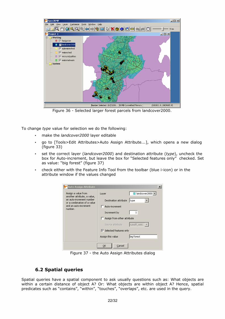
• Change the value for “Layer” to “Selection” from the drop down list, and set the other values in such a way that we retain areas larger that 1ha (figure 35). 26 forest areas should be selected now (Figure 36).

21/32

Figure 34 - The query builder of Simple Query.

Figure 35 - Selecting only larger parcels.

To change type value for selection we do the following:

• make the landcover2000 layer editable

• go to [Tools>Edit Attributes>Auto Assign Attribute...], which opens a new dialog (figure 33)

• set the correct layer (landcover2000) and destination attribute (type), uncheck the box for Auto-increment, but leave the box for “Selected features only” checked. Set as value: “big forest” (figure 37)

• check either with the Feature Info Tool from the toolbar (blue i-icon) or in the attribute window if the values changed

6.2 Spatial queries

Spatial queries have a spatial component to ask usually questions such as: What objects are within a certain distance of object A? Or: What objects are within object A? Hence, spatial predicates such as “contains”, “within”, “touches”, “overlaps”, etc. are used in the query.

22/32

Figure 36 - Selected larger forest parcels from landcover2000.

Figure 37 - the Auto Assign Attributes dialog

As an example for a spatial query we need to know what landcover2000 parcels are within 100 meters of the river network, since the river may have been contaminated by some chemicals. To answer the question we will not use “Simple Query”, which could be used as well to perform the task, but we will use “Spatial Query”. However, first we need to extract the rivers.

• Open [Tools>Queries>Attribute Query] (figure 38, left)

• set the dialog fields as follows: i) source layer: waternetwork, ii) attribute: type_axe, iii) relation: “=”, iv) and in the value field type “river”, v) keep “create a new layer for results” checked

Now a new layer called “waternetwork-=” is create that contains rivers only. Rename this layer to “river”. Now we perform the spatial query

• Open [Tools>Queries>Spatial Query] (figure 38, right)

• set the dialog fields as follows: i) Source layer: landcover2000, ii) relation: is within distance, iii) Mask layer: river, iv) parameter: 100.0, v) keep “create a new layer for results” checked

The result of this query is returned in the new layer named “landcover2000-is within distance' (figure 39), which contains 646 parcels. This value can be derived from the dialog that opens if “Layer properties...” from the layer mouse menu is chosen.

23/32

Figure 38 - left: Attribute Query dialog, right: Spatial Query dialog

Figure 39 - Land parcels within 100m distance to rivers.

Exercise 4

Exercise 4a

Which landcover2000 parcels of the type “big forest” are within 100 meters of the rivers.

Note: You should find 20 parcels.

Exercise 4b

Which are the hedges (from layer hedgerows) which “touch” grassland parcels (from layer landcover2000)?

Write down their total length and display the result in a new layer.

Note: To obtain the total length, i.e. the sum, you can use the function: [Tools>Statistics>Layer Attribute Statistics...] that calculates statistics for any attribute value. An alternative is to use the function [Tools>Statistics> Layer Statistics...] that calculates geometric statistics only. The number of hedges should be 523, and the calculated total length should be 42'177.79m.

7. Creating and editing geometry data

Before starting with data creation and editing we need to load our basedata:

• Open the rasters files F018_024.TIF and F018_025.TIF.

• Modify the watershed styling so that the topographic maps can be seen.

• Extract in new layer those features of the waternetwork dataset that attribute value of type_axe is equal to rivers. Name this layer rivers. (see the section on Attribute Queries)

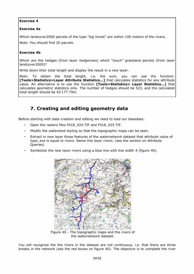
• Symbolize the new layer rivers using a blue line with line width 4 (figure 40).

You will recognize the the rivers in the dataset are not continuous, i.e. that there are three breaks in the network (see the red boxes on figure 40). The objective is to complete the river

24/32

Figure 40 - The topographic maps and the rivers of the waternetwork dataset.

network by creating new features based on the topographic map.

• Make all layers except rivers un-selectable (layer mouse menu)

• Zoom to the north red box

• Make rivers editable

• Use the draw line tool to create a new line If necessary reshape the line

• by adding,

• moving, or

• deleting vertices.

The keyboard shortcut functions mey be useful if one needs to zoom or pan while a drawing tool is activated. See under [Help>Shortcut Keys] what functions are available.

If you have drawn the line we need to ensure that the (drawn) segments touch each other. Zoom in and use the Snap Vertices Tool by drawing a box around the end points of the segments.

Before snapping After snapping

Next we need to set the attributes of the newly drawn segments.

Use the Feature Info Tool from the toolbar to display the attributes of each new segment.

Put the value “river” into the type_axe field for each new river segment (figure 41).

If you are done with editing you should save the dataset. You can store the data in a file or in a database, such as PostGIS. To store the data in a file chose from the mouse layer context menu [Save Dataset As...].

How to store data in PostGIS will be describe later in Part II. However we note that storing in a database requires to have a unique key. If no “gid” attribute exists in you dataset that could hold as a access key create one and assign unique values (see Part II - Section 1.3.1) - otherwise (i.e. a “gid” attribute exists already) assign unique values to the newly created segments only. Note: the sorting of the values in a table column may help you to find out if a value is unique.

25/32

Figure 41

II - Using OpenJUMP with PostGIS

1 OpenJUMP and PostGIS

1.1 Creating a database

The following step to create a new server is not necessary for the OGRS 2009 workshop since everything is prepared already. Otherwise...

Start the pgAdmin tool that is used to manage the PostgreSQL database.

Go to [File> Add Server...]

Apply the following settings:

Name : localhost

Host : localhost

Mainteance DB : postgres

Username : postgres

Password : leave empty (or: postgres)

DB restrictions: leave empty

Service : leave empty

You should obtain database view (figure 43). Figure 42 - connecting to a database server

Figure 43 - the pgAdmin interface

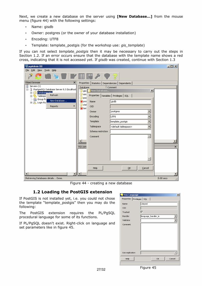
Next, we create a new database on the server using [New Database...] from the mouse menu (figure 44) with the following settings:

• Name: gisdb

• Owner: postgres (or the owner of your database installation)

• Encoding: UTF8

• Template: template_postgis (for the workshop use: gis_template)

If you can not select template_postgis then it may be necessary to carry out the steps in Section 1.2. If an error occurs ensure that the database with the template name shows a red cross, indicating that it is not accessed yet. If gisdb was created, continue with Section 1.3

1.2 Loading the PostGIS extension

If PostGIS is not installed yet, i.e. you could not chose the template “template_postgis” then you may do the following:

The PostGIS extension requires the PL/PgSQL procedural language for some of its functions.

If PL/PgSQL doesn't exist. Right-click on language and set parameters like in figure 45.

27/32

Figure 44 - creating a new database

Figure 45

Now, let's load the PostGIS functions.

Open SQL query builder

1. Load the file lwpostgis.sql and execute it (figure 46)

2. Load spatial_ref_sys.sql

Now we are ready to import and to work with spatial data and features in PostgreSQL.

1.3 Using PostGIS

1.3.1 Populating the database

Preparing the data

Create a new project in OpenJUMP and load the following files:

Open shapefiles :"waternetwork.shp", "watershed.shp"

For each layer:

• In PostGIS tutorials often the geometry attribute is often called: “the_geom”. In our query examples below we will use “geometry” instead of “the_geom”. However, if you wish to use “the_geom”, then do the following: Open the layer schema and change the name of the geometry attribute to “the_geom”. (figure 47)

• For storage of the data we need a unique access key for every object. Such key is in our case an attribute that contains a value only once. If such attribute is not already existing3, we add an attribute “gid” of type integer to the dataset/ layer. Populate it with function [Tools>Edit Attributes>Auto Assign Attributes...] using the option “Auto-Increment”. Now, every object should have a unique key value.

• Change the SRID4 to the (French) projection of our dataset: EPSG:27582 - NTF(Paris)/Lambert II (étendu) by using [Layer>Change SRID...] (figure 48). Set value “27582”. If the SRID number is not known, it can be also set to “-1”.

3 Note, the FID attribute can not be used for this, since it is a dynamic attribute that is newly generated each time.

4 SRID: Spatial Reference ID

28/32

Figure 46

Storing the layers in the PostGIS database “gisdb”

Select the layer to import

chose from the layer context menu [Save Dataset As...]

In the dropdown list for the storage format choose PostGIS Table. (Note that this option is only available when the OpenJUMP PostGIS plugin is installed)

Figure 49 shows parameters and the option to create a new table named watershed in gisdb database.

During the OGRS 2009 workshop use “postgres” as password.

Add also the waternetwork dataset to the database.

1.3.2 Display data from PostGIS in OpenJUMP

Open [File>Open...] and select “Data Store Layer” from the list of options on the left panel. (figure 50)

In the new dialog click on the Connection Manger button on the left side (figure 50).

Again a new dialog will open to add a database connection (figure 52). Click on the [Add] button and fill in the fields as shown in figure 51 (OGRS pw: “postgres”).

Click [ok], and to return from the Connection Manager dialog (figure 52) click again on [ok], since we are already connected to the database.

29/32

Figure 47 - Using “the_geom” instead of “geometry”.

Figure 49 - Committing data to the PostGIS database.

Figure 48 - Set the SRID.

Figure 50 - Loading data from a data store

If available select from the drop down list the dataset you want to load (figure 53). Otherwise type the name in the “Dataset” field.After clicking ok, the layer should be loaded in OpenJUMP.

Load from the database the layers waternetwork and water-shed.

Note: If data are loaded with the Data Store method then not all data are loaded in OpenJUMP, but only those data that are covered by the current map view (i.e. extent). Hence, if operations/calculations should be performed on the complete dataset, then one needs to zoom to the full dataset (layer mouse menu function: “Zoom to Layer”) and eventually duplicate all layer objects into a new layer first (from the mouse menu chose: 1. Zoom to Layer, 2. Select current layer items, and 3. [Layer>Replicate Selected Items]). That OpenJUMPs is displaying data in a dynamic fashion from datastores is sometimes recognizable by a small clock icon that shortly shows up next to the layer name. This icon indicates when data are requested from the database that are within the current map extents.

1.3.3 Performing SQL queries

To filter data in a PostGIS database and display the results in OpenJUMP you can use the Datastore Query function that provides a small GUI to run SQL syntax. Open the dialog under [Layer>Run Datastore Query] (figure 54).

30/32

Figure 53 - Open a dataset from a datastore

Figure 52 - Connection ManagerFigure 51 - Adding a database connection.

If there are no databases provided in the “connection” drop down list, then you need to add a connection with the button shown on the right of the dialog. How to do that has been explained in the previous section.

Attribute queries can have this syntax:

SELECT ST_AsBinary(<geometry column>) AS the_geom, <column list> FROM <table> WHERE <column name>=<value>;5

An example in which we want to obtain all objects in the waternetwork dataset those type is equal to ditch is given in figure 55.

The query text is:

select ST_AsBinary(geometry) as geometry, type_axe, gid from waternetwork where type_axe='ditch';

5 If you perform this SQL query with pgAdmin's query tool, then you may replace ST_AsBinary by asewkt, i.e. write: select asewkt(geometry)...

31/32

Figure 54 - the Datastore Query Dialog to perform SQL queries in OpenJUMP.

Figure 55 - Selecting ditches from the waternetwork dataset.

In the second example we perform a spatial query that will return those river segments that have a certain length.

SELECT ST_AsBinary(geometry) AS geometry, type_axe, gid FROM waternetwork WHERE length(geometry) > 200;

Note that the length unit used here is metric (meters). The resulting layer should contain 35 waternetwork objects of length larger than 200m.

Exercise 5

After saving landcover2000 in PostGIS find those parcels that - are grassland, and - have an area greater than 2 hectares

The result must be display in OpenJUMP and layer must contains three columns: gid, type and area.

Notes: - function area is area(<geometry column>)- 10'000 square meters is equal to 1 hectareDon't forget that SRID value is 27582 and the unit is metric.

It is also possible to perform queries that include several search statements. This is achieved by using the “and” statement.

In the example below we want to select parcels from landcover2000 dataset that are contained in areas of wsmunicipalities that have the municipality name “QUEMPERVEN”.

SELECT ST_AsBinary(landcover2000.geometry) as geometry, landcover2000.type FROM landcover2000, wsmunicipalities WHERE contains(wsmunicipalities.geometry, landcover2000.geometry) AND wsmunicipalities.name_mun='QUEMPERVEN';

The same query can be performed with pgAdmin. pgAdmin also allows to create very complex queries. However, when performing queries in pgAdmin we can not display the query output as a geographic data layer and we need to formulate the query like this:

SELECT landcover2000.type FROM landcover2000, wsmunicipalities WHERE contains(wsmunicipalities.geometry, landcover2000.geometry) AND wsmunicipalities.name_mun='QUEMPERVEN';

An extensive introduction and more examples on how to perform SQL queries with PostGIS will be given in the upcoming PostGIS book: “PostGIS in Action” by R.O. Obe and L.S. Hsu (see http://www.manning.com/obe/). On our webpage openjump.org can be found also a second OpenJUMP - PostGIS tutorial on mineral targeting by Ravi Kumar, which presents further examples.

32/32