offshore wind energy study and its impact on …

Clemson UniversityTigerPrints

All Dissertations Dissertations

12-2013

OFFSHORE WIND ENERGY STUDY ANDITS IMPACT ON SOUTH CAROLINATRANSMISSION SYSTEMTingting WangClemson University, [email protected]

Follow this and additional works at: https://tigerprints.clemson.edu/all_dissertations

Part of the Electrical and Computer Engineering Commons

This Dissertation is brought to you for free and open access by the Dissertations at TigerPrints. It has been accepted for inclusion in All Dissertations byan authorized administrator of TigerPrints. For more information, please contact [email protected].

Recommended CitationWang, Tingting, "OFFSHORE WIND ENERGY STUDY AND ITS IMPACT ON SOUTH CAROLINA TRANSMISSIONSYSTEM" (2013). All Dissertations. 1216.https://tigerprints.clemson.edu/all_dissertations/1216

https://tigerprints.clemson.edu?utm_source=tigerprints.clemson.edu%2Fall_dissertations%2F1216&utm_medium=PDF&utm_campaign=PDFCoverPages

https://tigerprints.clemson.edu/all_dissertations?utm_source=tigerprints.clemson.edu%2Fall_dissertations%2F1216&utm_medium=PDF&utm_campaign=PDFCoverPages

https://tigerprints.clemson.edu/dissertations?utm_source=tigerprints.clemson.edu%2Fall_dissertations%2F1216&utm_medium=PDF&utm_campaign=PDFCoverPages

https://tigerprints.clemson.edu/all_dissertations?utm_source=tigerprints.clemson.edu%2Fall_dissertations%2F1216&utm_medium=PDF&utm_campaign=PDFCoverPages

http://network.bepress.com/hgg/discipline/266?utm_source=tigerprints.clemson.edu%2Fall_dissertations%2F1216&utm_medium=PDF&utm_campaign=PDFCoverPages

https://tigerprints.clemson.edu/all_dissertations/1216?utm_source=tigerprints.clemson.edu%2Fall_dissertations%2F1216&utm_medium=PDF&utm_campaign=PDFCoverPages

mailto:[email protected]

OFFSHORE WIND ENERGY STUDY AND ITS IMPACT ON SOUTH

CAROLINA TRANSMISSION SYSTEM

A Dissertation

Presented to

the Graduate School of

Clemson University

In Partial Fulfillment

of the Requirements for the Degree

Doctor of Philosophy

Electrical Engineering

by

Tingting Wang

December 2013

Accepted by:

Dr. Elham B. Makram, Committee Chair

Dr. Ian Walker

Dr. Hyesuk Lee

Dr. Keith Corzine

ii

ABSTRACT

As one of the renewable resources, wind energy is developing dramatically in

last ten years. Offshore wind energy, with more stable speed and less environmental

impact than onshore wind, will be the direction of large scale wind industry. Large

scale wind farm penetration affects power system operation, planning and control.

Studies concerning type III turbine based wind farm integration problems such as

wind intermittency, harmonics, low voltage ride through capability have made great

progress. However, there are few investigations concerning switching transient

impacts of large scale type III turbine based offshore wind farm in transmission

systems. This topic will gain more attention as type III wind generator based offshore

wind farm capacity is increasing, and most of these large scale offshore wind farms

are injected into transmission system. As expected to take one third of the whole wind

energy by 2030, the large offshore wind energy need to be thoroughly studied before

its integration particularly the switching transient impacts of offshore wind farms.

In this dissertation, steady state impact of large scale offshore wind farms on

South Carolina transmission system is studied using PSSE software for the first time.

At the same time, the offshore wind farm configuration is designed; SC transmission

system thermal and voltage limitation are studied with different amount of wind

energy injection. The best recommendation is given for the location of wind power

injection buses.

Switching transient also impacts is also studied in using actual South Carolina

transmission system. The equivalent wind farm model for switching transient is

iii

developed in PSCAD software and different level of wind farm penetration evaluates

the transient performance of the system.

A new mathematical method is developed to determine switching transient

impact of offshore wind farm into system with less calculation time. This method is

based on the frequency domain impedance model. Both machine part and control part

are included in this model which makes this representation unique. The new method

is compared with a well-established PSCAD method for steady state and transient

responses. With this method, the DFIG impact on system transients can be studied

without using time-domain simulations, which gives a better understanding of the

transient behaviors and parameters involved in them.

Additionally, for large scale offshore wind energy, a critical problem is how to

transmit large offshore wind energy from the ocean efficiently and ecumenically. The

evaluation of different offshore wind farm transmission system such as HVAC and

HVDC is investigated in the last chapter.

iv

DEDICATION

This dissertation is dedicated to my parents, Ouguang Wang & Qizhen Luo,

and my fiancé Xufeng Xu.

v

ACKNOWLEDGMENTS

I would like to express my sincerest gratitude to my advisor and mentor Dr.

Elham B. Makram not only for her guidance, caring, encouragement and patience

throughout my research, but also always willing to help and give her best suggestions

for my life.

I would like to thank Dr. Adly. A. Girgis, who is an example of industrious,

righteous, conscientious professor. Without Dr.Makram and him, I would have no

chance to continue my study in the United State. Dr.Markam and Dr. Girgis are like

my family in Clemson.

I would like to thank Dr. Ian D. Walker, Dr. Hyesuk Lee and Dr.Keith

Corzine for help about my research and being my committee members.

I would like to thank Dr. Ramtin Hadidi for his guidance and help about my

research. I would like to thank Laura B Kratochvill for her help to review my

dissertation, and Drenda Whittiker Stutts for her help and friendship.

I would like to thank all my colleagues in the power group for their friendship.

I would like to thank my fiancé Xufeng Xu, without whom this cannot be

possible.

Finally I would like to thank my parents for their patience and their emotional

and financial support throughout my life.

https://www.facebook.com/drendawhittiker?hc_location=timeline

vi

TABLE OF CONTENTS

Page

TITLE PAGE .................................................................................................................... i

ABSTRACT ..................................................................................................................... ii

DEDICATION ................................................................................................................ iv

ACKNOWLEDGMENTS ............................................................................................... v

LIST OF TABLES ........................................................................................................... x

LIST OF FIGURES ........................................................................................................ xi

CHAPTER

1. INTRODUCTION ......................................................................................... 1

1.1 Motivation ........................................................................................... 1

1.2 Research Background ......................................................................... 2

1.3 Steady State Impact............................................................................. 4

1.4 Switching Transient ............................................................................ 6

1.5 Offshore Wind Farm Switching Transient .......................................... 9

1.6 Frequency Domain Impedance Matrix ............................................. 11

1.7 Offshore Wind farm HVAC and HVDC

Transmission System ......................................................................... 12

1.8 Research Objectives, Contributions and

Structures .......................................................................................... 13

2. OFFSHORE WIND FARMS STEADY STATE

IMPACT ON SOUTH CAROLINA

TRANSMISSION SYSTEM ................................................................. 16

2.1 Steady State Analysis Phase I .......................................................... 16

2.1.1 Description of Offshore Wind ................................................ 16

2.1.2 Offshore Wind Farm Configuration ........................................ 19

2.1.3 Generation Reduction .............................................................. 20

2.1.4 Wind Farm Integration Requirement ..................................... 20

2.1.5 The Simulation and Results Analysis...................................... 21

2.2 Steady State Analysis Phase II ......................................................... 22

2.2.1 Analysis of Simulation Results ............................................... 25

2.2.2 Suggestion for Second Stage ................................................... 26

2.3 Steady State Analysis Phase III ....................................................... 28

vii

Table of Contents (Continued)

Page

2.3.1 Analysis of Simulation Results ............................................... 29

2.3.2 Suggestion for the Third Stage ................................................ 31

2.3.3 Testing of 2009 Light Load Base Case ................................... 34

3. OFFSHORE WIND FARM SWITCHING

TRANSIENT STUDY ........................................................................... 36

3.1 The Equivalent Wind Farm Model .................................................. 37

3.1.1 Offshore Wind Farm Collecting Grid for

Transient Study ....................................................................... 37

3.1.2 Concept Equivalent Modeling for

Transient Study ....................................................................... 37

3.1.3 Equivalent Procedure ............................................................. 39

3.1.4 Equivalent Model Verification ............................................... 41

3.2 Wind Farm Switching Transient Impact on

Power System................................................................................... 44

3.2.1 40MW Wind Farm Integrated SC System

Units ........................................................................................ 44

3.2.2 Cable Energizing in Wind Farm Equivalent .......................... 46

3.2.3 Three-Phase Fault at Different Locations

in a Wind Farm ...................................................................... 47

3.3 Conclusions ...................................................................................... 51

4. SWITCHING TRANSIENT IMPACT OF OFFSHORE

WIND FARM ON POWER SYSTEM ................................................. 52

4.1 System Description .......................................................................... 53

4.1.1 Offshore Wind Farm Equivalent Model .................................. 53

4.1.2 South Carolina Reduced System ............................................. 54

4.2 Computer Modeling Procedure ........................................................ 57

4.2.1 South Carolina Reduced System ............................................. 57

4.2.2 Equivalent PSCAD Model Imported From

PSSE ....................................................................................... 58

4.2.3 South Carolina Intentional Islanded Power

System ..................................................................................... 60

4.3 Case Simulation ............................................................................... 62

4.3.1 Capacitor Bank Switching and the Three-

Phase Fault .............................................................................. 62

4.3.2 Offshore Wind Farm Disconnection ...................................... 63

viii


Page

4.3.3 Three-Phase Fault and its Clearance in the

Intentional Islanded System .................................................... 65

4.4 Conclusions and Future Work ......................................................... 67

5. FREQUENCY DOMAIN ANALYSIS OF THE

IMPACT OF THE OFFSHORE WIND FARM

SWITCHING TRANSIENT .................................................................. 68

5.1 Introduction ...................................................................................... 68

5.2 The Approach................................................................................... 70

5.3 The Derivation of the Induction Generator ...................................... 72

5.3.1 Machine Park Transformation ................................................ 73

5.3.2 The Stator Flux Oriented ........................................................ 80

5.3.3 Feed Forward Decouple Control ............................................. 84

5.3.4 Grid Side PWM Converter and Control .................................. 87

5.3.5 Combination of the Two Parts ................................................ 91

5.4 The Simulation Results of the Zbus Matrix ..................................... 98

6. ECONOMIC EVALUATION AND DESIGN

CONSIDERATION OF HVAC AND HVDC

OFFSHORE WIND FARM ................................................................. 102

6.1 Introduction .................................................................................... 102

6.2 Configurations of Offshore Wind Farms

Transmission Systems ................................................................... 106

6.2.1 Plan A Directly Connected Configuration ............................ 106

6.2.2 Plan B the HVAC Transmission System............................... 107

6.2.3 Plan C the HVDC Transmission System .............................. 110

6.3 Offshore Wind Energy System

Components and Costs ................................................................... 114

6.3.1 Offshore Wind Turbine Foundation Cost.............................. 114

6.3.2 Offshore Substation and Converter Station ........................... 118

6.3.3 Submarine Cable (HVAC and HVDC) ................................. 120

6.3.4 The Summary of Offshore Wind Farm

Capital Costs ......................................................................... 121

6.4 The Steady State and Switching Transient Performance ............... 123

6.4.1 HVDC Connection for Offshore Wind Farm ........................ 123

6.4.2 HVAC Connection for Offshore Wind Farm ........................ 125

6.5 Conclusions and Summary ............................................................ 126

APPENDICES ............................................................................................................. 130

A: Table 1 Transformer Parameters for Phase II .................................................. 130

B: Table 2 Data for the GE 3.6 MW Wind Turbine ............................................. 131

ix


Page

C: Table 3 Transformers Specification ................................................................. 132

REFERENCES ............................................................................................................ 133

x

LIST OF TABLES

Table Page

Table 1.1 Offshore wind capacity by Nation- December 2011 ..................................... 3

Table 1.2 Offshore wind farm projects in the United States .......................................... 4

Table 1.3 Offshore wind farm integration regulations ................................................... 4

Table 2.1 List of coastal 115 kV buses ........................................................................18

Table 2.2 Case list used for each of the three base case power flow ........................... 21

Table 2.3 Recommend 115 kV interface buses ........................................................... 22

Table 2.4 Wind energy distribution ratio ..................................................................... 25

Table 2.5 Recommended interface buses..................................................................... 26

Table 2.6 Suggested case using three 115kV interface buses ...................................... 27

Table 2.7 Wind energy distribution ratio ..................................................................... 29

Table 2.8 System injection limitation .......................................................................... 30

Table 2.9 List of Santa Cooper’s 230 kV coastal buses .............................................. 30

Table 2.10 Distribution of wind power between interface buses ................................. 31

Table 2.11 Critical generators for congestion at Winyah Bay area ............................. 32

Table 2.12 Suggested new transmission lines.............................................................. 33

Table 2.13 System injection limit using different set of 115 kV buses ....................... 33

Table 2.14 Cases with new transmission lines............................................................. 34

Table 2.15 Voltage violations at light load .................................................................. 35

Table 2.16 Recommended interface buses for injecting 3080 M ................................ 36

Table 3.1 DFIG detailed model and equivalent model ................................................39

Table 3.2 Comparison of two models .......................................................................... 42

Table 3.3 Harmonic components in the wind farm current ......................................... 45

Table 3.4 Comparison of three-phase fault at different locations ................................ 48

Table 4.1 SC reduced system data ...............................................................................54

Table 4.2 Intentional islanded system data .................................................................. 55

Table 4.3 Equivalent cases summaries ........................................................................ 59

Table 6.1 Impact of depth and distance on cost .........................................................103

Table 6.2 Offshore wind farm and its cost ................................................................. 104

Table 6.3 Wind turbine components and their price .................................................. 115

Table 6.4 Cost of different types of foundations ....................................................... 117

Table 6.5 Installation cost for wind turbines ............................................................. 118

Table 6.6 Wind farm projects online today with offshore substations ...................... 118

Table 6.7 Average cost of an HVAC offshore substation ......................................... 119

Table 6.8 Average cost of an HVDC offshore substation ......................................... 120

Table 6.9 HVAC and HVDC submarine cable cost .................................................. 121

Table 6.10 Summary of offshore wind farm configuration costs .............................. 121

Table 6.11 Summary of the offshore wind farm cost breakdown.............................. 122

Table 6.12 Offshore wind farm online capital cost breakdown ................................. 122

Table 6.13 Summary of the difference configuration ................................................ 128

xi

LIST OF FIGURES

Figure Page

Figure 1.1 Map of South Carolina with wind penetration ............................................. 5

Figure 1.2 Power system study time frame .................................................................... 7

Figure 1.3 Power system impedance matrix ................................................................ 11

Figure 2.1 Locations of wind farms in South Carolina ................................................16

Figure 2.2 Possible locations of the North Myrtle Beach wind farm .......................... 17

Figure 2.3 Possible location of the wind farm in Winyah Bay .................................... 18

Figure 2.4 Wind farm connection for Phase I .............................................................. 19

Figure 2.5 Wind power density of South Carolina ...................................................... 23

Figure 2.6 Illustrations of offshore wind farm locations ............................................. 23

Figure 2.7 Wind farm connection diagram .................................................................. 24

Figure 3.1 Wind farm configuration and aggregation .................................................38

Figure 3.2 Control blocks for DFIG ............................................................................ 41

Figure 3.3 The comparison of active power outputs between two models .................. 42

Figure 3.4 Interface bus voltage comparison ............................................................... 43

Figure 3.5 Interface bus current comparison ............................................................... 43

Figure 3.6 40MW equivalent wind farm integration ................................................... 44

Figure 3.7 40MW equivalent wind farm output voltage.............................................. 44

Figure 3.8 Current output of 40MW equivalent wind farm ......................................... 45

Figure 3.9 Power output of 40MW equivalent wind farm ........................................... 46

Figure 3.10 Cable energizing wind farm ..................................................................... 46

Figure 3.11 Voltage at the substation at cable switching............................................. 47

Figure 3.12 The three-phase fault in a wind farm ........................................................ 47

Figure 3.13 Three-phase fault currents at different locations ...................................... 48

Figure 3.14 Wind farm injected fault current at different location fault ..................... 49

Figure 3.15 Three-phase fault power at different locations ......................................... 49

Figure 3.16 Three-phase fault voltage RMS at different locations .............................. 50

Figure 3.17 Recovery voltage after the faults have cleared ......................................... 51

Figure 4.1 Wind farm configuration and aggregation .................................................56

Figure 4.2 Intentional islanded zone ............................................................................57

Figure 4.3 System modeling in PSCAD ......................................................................58

Figure 4.4 Data imported from PSSE to PSCAD ........................................................59

Figure 4.5 Intentional islanded zone and tie lines........................................................60

Figure 4.6 Equivalent for the rest system ....................................................................61

Figure 4.7 Voltage wave of the capacitor switching....................................................62

Figure 4.8 Voltage wave of three-phase fault ..............................................................63

Figure 4.9 Voltage wave of OWF disconnection.........................................................63

Figure 4.10 Capacitor bank inrush current at bus P .....................................................64

Figure 4.11 Frequency analysis of the capacitor inrush current at bus P ....................65

Figure 4.12 Transient recovery voltage of the OWFs supplied system .......................65

Figure 4.13 Transient recovery voltage of the conventional generator system ...........66

Figure 4.14 Frequency analysis of the transient recovery voltage ...............................66

Figure 5.1 Grid side converter and machine side converter ........................................71

Figure 5.2 Algorithm of Zbus derivation ....................................................................... 71

xii

List of Figures (Continued)

Figure Page

Figure 5.3 Machine windings ...................................................................................... 72

Figure 5.4 Equivalent circuits for rotor and stator winding ......................................... 72

Figure 5.5 The doubly fed induction generator block diagram ................................... 83

Figure 5.6 Feed forward decoupled controller ............................................................. 84

Figure 5.7 DFIG with feed forward decoupled controller ........................................... 84

Figure 5.8 Feed forward decouple controller ............................................................... 86

Figure 5.9 DFIG grid side converter ............................................................................ 88

Figure 5.10 DFIG grid side converter block diagram .................................................. 89

Figure 5.11 Decoupled control scheme for the grid side converter ............................. 90

Figure 5.12 Decoupled control .................................................................................... 91

Figure 5.13 Angle difference between stator and grid converter reference ................. 92

Figure 5.14 Configuration of the two parts impedance for DFIG ............................... 94

Figure 5.15 Equivalent impedance of DFIG model ..................................................... 97

Figure 5.16 Steady state results for two models .......................................................... 99

Figure 5.17 Comparison of two models short circuit results ..................................... 100

Figure 5.18 Comparison of two models short circuit results ..................................... 100

Figure 6.1 EWEA data for wind energy production and capacity .............................102

Figure 6.2 Offshore wind and onshore wind cost (EWEA data) ............................... 104

Figure 6.3 Direct connection of an offshore wind farm ............................................. 107

Figure 6.4 HVAC transmission systems for an offshore wind farm ......................... 108

Figure 6.5 Shows the HVDC wind energy transmission scheme .............................. 112

Figure 6.6 Wind turbine components......................................................................... 115

Figure 6.7 Different types of foundations used in offshore wind projects ................ 116

Figure 6.8 Offshore wind farm foundations (EWEA) ............................................... 117

Figure 6.9 HVDC Transmission System ................................................................... 124

Figure 6.10 Output power of the offshore wind farm with an HVDC system........... 124

Figure 6.11 AC and DC of inverter in the HVDC transmission system .................... 124

Figure 6.12 HVAC transmission system ................................................................... 125

Figure 6.13 Output power of the offshore wind farm with the HVAC system ......... 125

Figure 6.14 Output voltage of offshore wind farm with the HVAC system.............. 126

1

CHAPTER ONE

INTRODUCTION

1.1 Motivation

Large scale offshore wind farms affect the integrated system transient by

changing the grid configuration. Wind farms based on Type III wind turbines have a

large number of energy storage devices including induction generators, converters,

and transformers as well as submarine cables. The integration of such complicated

network into system motivates the analysis of the transient impact of the wind farm as

switching operations, for example load switching, capacitor bank switching, and small

fault, and frequently occur. The Transient over Voltage (TOV), inrush current, and

high frequency transient components are used to determine the insulation and

protection coordination [1]. Failure to provide accurate information for those settings

in a power system can cause overheating or damage, protection malfunction or loss of

system stability after a fault [2]. Thus, it is critical to analysis the impact of the

offshore wind farm impact on system switching transient.

Due to the development of digital computers, system transient studies

requiring a device detailed model are able to be conducted using an appropriate

discrete time program. However, it is difficult to simulate wind farm integrated

systems, given their number of electrical storage devices connected in complicated

configuration Thus, such as study needs an appropriate equivalent model. This

problem is addressed in Chapter 2 of this dissertation.

2

Additional issues from the perspective of a wind farm project protection

engineer involve the accessibility of the system data and decisions concerning the

TOV or high frequency impact can be decided for protection devices installed on the

system side.

This dissertation focuses on answering those questions in relation to the

impact of offshore wind farm penetration impact on transmission system, including

steady state impact and switching transient impact.

1.2 Research Background

Before explaining the goals of this dissertation, the status of wind energy

development and its future are discussed. The wind industry is currently experiencing

record growth. Table 1.1 shows the offshore wind farm capacity installed in different

countries in the world by the end of 2011. The worldwide wind energy installation

capacity reaches 296.255 Giga Watt (GW) by the end of June 2013, adding 13.98GW

in the first six month of that year [3]. In the second half of 2013, an additional 22GW

is expected to be constructed. Offshore wind saw it best growth in 2013, adding

1.08GW accounting for 7.1GW of the world’s total energy capacity. After the

erection of the world’s first offshore wind farm, the Vindeby Farm in Denmak with a

capacity of 4.95MW installation capacity-built, other countries began developing

similar structures [4]. Expanding since 2006, 4,600 Mega Watts (MW) of offshore

wind farms were operating worldwide by mid-2012, the majority of the offshore wind

farms online in Europe. Though a small amount compared with the onshore wind,

3

offshore wind shows great promise, with projections suggesting it will be responsible

for one third of the world’s wind energy by 2030[3].

Table 1.1 Offshore wind capacity by Nation- December 2011

Nation Consented

(MW)

Construction

(MW)

Operational

(MW) Total (MW)

United Kingdom 1,257 2,239 1,341 4,837

Denmark 436 0 856 1,292

Belgium 529 148 195 872

Netherlands 3,037 0 228 3,265

Sweden 1,531 0 161 1,692

Germany 7,909 600 121 8,630

Finland 768 0 30 798

Ireland 1,100 0 25 1,125

Norway 407 0 2 409

Estonia 700 0 0 700

France 108 0 0 108

Total 17,782 2,987 2,959 23,728

Data from 4COffshore, industry press

The offshore wind industry in the US has not seen the dramatic growth as the

rest of the world has [5]. The projects in the United States under development are

mainly in the North Atlantic Ocean and on the Great Lake [6]. Even though the

National Renewable Energy Laboratory (NREL) estimates that U.S. offshore winds

have a gross potential generating capacity four times greater than the nation’s present

electric capacity, at present there is no operating offshore wind farm in the United

States[7]. The obstacles for offshore wind development are not only geographical and

technological but also financial, regulatory and supplying chain as well. The most

advanced proposed offshore wind projects in the US are listed in the Table 1.2.

4

Table 1.2 Offshore wind farm projects in the United States

Offshore Wind Farm Location Nameplate Capacity

Cape Wind Massachusetts 468MW

Coastal Point Energy Galveston Texas 150MW

Blue water Wind Delaware 450MW

Deepwater Wind Rhode Island 415MW

Garden State Offshore Energy New Jersey 350MW

Before integration, the generated wind power or voltage has to meet

requirements such as power reliability standards, and flicker emission standards

because of switching operations and voltage reduction during faults [4]. Since the

regulations vary across countries, it is important to beware of the specific ones for the

interconnected power system under consideration. Table 1.3 illustrates some wind

farm integration regulations [4].

Table 1.3 Offshore wind farm integration regulations

Regulations

IEEE Standard 1001

MEASNET guide line

IEC 61400-21

1.3 Steady State Impact

South Carolina possesses potential offshore wind energy more than twice the

amount of its consumption [8]. In 2009, Santee Cooper, a local South Carolina (SC)

utility, proposed an offshore wind farm project along the SC coastal line to the

5

Department of Energy (DOE). This proposed project aims to exploit the green energy

from the Atlantic Ocean along South Carolina the coastal line as shown in Figure 1.1.

The two wind farms proposed are at North Myrtle Beach and Winyah Bay. The

project is composed of three phases. For Phase I, 80 MW wind energy from state

waters will be injected at two locations near the shore of South Carolina by 2013. For

Phase II, an additional 1GW of wind energy from federal waters will be injected by

2020, while Phase III proposed to add another 2 GW of wind energy is to be added to

the system by 2030.

The Clemson University Electric Power Research Associate (CUEPRA) has

been funded to investigate the steady state impact of different amounts offshore wind

energy on the SC transmission system [9], the issue addressed in Chapter 2 of this

dissertation. The steady state technical report completed in 2011 by CUEPRA

included three sections, each focusing on a different amount of wind injection. Results

from this study are the initial points for further investigating the switching transient

impact of SC offshore wind farms.

Figure 1.1 Map of South Carolina with wind penetration

6

1.4 Switching Transient Modeling and Solver

The power system is a complicated dynamic one, interconnected through

numerous coupled energy storage components; it has to secure the qualified economic

electrical energy to be delivered from the generator side to the load side at all the time.

At the same time it has to sustain synchronization under persistent random

disturbances [10][11].

When the system is subjected to a disturbance such as a fault, excessive

currents or voltage variations result. The period time after the power system

experiences a disturbance is defined as a transient [2][12]. If it is a small disturbance,

such as load shedding or restoring, the system can adjust itself, while large

disturbances such as a short-circuit on a transmission line, loss of a large generator or

load, or loss of a tie between two subsystems, cause system responses such as a new

state of operating equilibrium or a large excursion of generator rotor angle which

might degrade the synchronization [13][14]. The ability of a power system to remain

in operating equilibrium or regain a stable equilibrium is defined as power system

stability. The loss of system stability can cause significant economic loss or some

other disaster in a few seconds [15]. The prediction of such issues, which is the main

objective of any power system transient study, is essential in the design of power

systems, specifically for deriving the component ratings and optimizing controller and

protection settings.

An effective way to analyze system transient is to categorize various models

by their corresponding time scales. In light of the transient period involved, the power

system study can be categorized as electromagnetic transient or electromechanical

transient. Electromechanical transients refer to interactions between the electrical

7

energy stored in the system, while electromagnetic transient is defined by the

interaction between the electrical field of capacitance and the magnetic field of

inductances in the power system. As shown in the Figure 1.2, transient process

usually lasts within one second and can be categorized

10-6

10-4

10-2

100

102

104

10-8

10-6

10-4

10-2

100

102

104

0

Time(s)

Lighting Transient

Switching Transient

Subsynchronous Resonance

Dynamic Stability

Tie Line

Regulation

Daily Load Management,

Operation Actions

Transient Stability

Figure 1.2 Power system study time frame

Switching transient is usually caused by the operations in a power system such

as capacitor bank switching, load switching, or different types of fault or its clearance

[2].Also, energizing various devices in a power system such as transformer energizing

or cable energizing are very common triggers for this type of transients. The concerns

resulting from a switching transient include high magnitude transient voltage or

inrush current with frequency components arranging from the fundamental frequency

up to 20 kHz [2]. These can cause stress on system insulation, affect protection

settings in relays, influence the power quality, the damage equipment in the system or

violate stability in the worst case.

8

An electromagnetic transient study is critical for in a power system in the area

of insulation coordination, overvoltage studies caused by very fast transients, surge

arrestor ratings, sub-synchronous resonance and Ferro resonance, relay coordination,

transformer saturation effects studies, electrical filter design, control system design

etc.

The research reported in this dissertation focuses on switching transient

analysis, part of which is the electromagnetic transient study; the time length of a

switching transient ranges from 1 ms to less than 1 sec [2]. However, transient

stability is not included in this research.

The modeling of the system must be appropriate for the scope of the study. It

is critical to categorize the phenomena by the time scale under consideration [2]. For

example, steady state power flow problems can be formulated as a set of nonlinear

algebraic equations based on current and voltage phasor in a frequency domain. The

solutions usually include Gauss-Seidel iterations, the Newton Raphson method, and a

decoupled power flow.

A switching transient study, due to power system’s composition of hundreds

and thousands of nonlinear devices such as generators and transformers, can be

described by nth

first order linear differential equations [12]. The study of a power

system transient primarily involves solving those equations in the frequency domain

and time domain. The analysis of an electromagnetic transient solves a set of

Kirchhoff’s laws based on first order differential equations. There are different

methods to solve differential equations.

There are several methods for solving differential equations. The Laplace

transform system is suitable for a frequency-focused study, but the calculations

9

dramatically increase as the system size changes. Transient network analysis (TNA)

and the HVDC simulator use an analogue computer to simulate the transient. This

dissertation focuses on the solution of electromagnetic transient problems in an

offshore wind farm penetrated power system. In addition, in second part of this

research, which focuses on the switching transient impact, uses PSCAD.

For the time domain algorithm the treat iterations is required, while numerical

algorithm, such as the Runge-Kutta method, involve a numerical stability problem

[16]. The development of the digital computer has led to more accurate and general

solutions provided by computer-aided programs. Software like PSCAD/EMTDC or

EMTP can provide the time domain solutions applicable for an electromagnetic

transient study.

EMTDC (PSCAD) and other EMTP-type programs are based on the principles

outlined in the classic 1969 paper by Hermann Dommel [17]. In this dissertation, the

time domain simulation is implemented in PSCAD. EMTDC then converts the system

into Norton equivalents, using numerical integration substitution to calculate transient

phenomena [17][18].

1.5 Offshore Wind Farm Switching Transient

The switching operations related to an offshore wind farms integrated system

could either be inside or outside the wind farm at the system side [19][20]. These

operations include starting up wind generators, energizing the transformers or

submarine cables and switching on or off the wind generators from the system. These

operations impact the power delivery from the wind farms to the system and the

10

power quality of the wind farm. Since the switching operations in a wind farm

connected system may be caused by the system devices, switching operations such as

capacitor bank switching may also influence the operation of the offshore wind farm.

Wind farm related research has focused on two primary areas, windmill

modeling and wind farm integration impact research. Based on wind generator

modeling, as it is known, today’s wind generators can be classified into four types in

today’s market [4]. This research in this dissertation concentrates on the Type III, the

Doubly Fed Induction Generator (DFIG). Based on past investigations, wind

generators can be modeled as steady-state-oriented models [21], transient-stability-

oriented models, or switching-transient-oriented models. The papers discussing wind

turbines modeling include [18][22][23][24]. The type of wind turbine used in this

research, the DFIG, has different types of control schemes such as direct torque

control as discussed in [25], current control based on the reference quantities used [26]

and the converter used[27][28]. As part of offshore wind farms, devices such as

breakers and submarine cables are required to be modeled for specific research

purpose. Papers discussing the modeling of those devices include [29], while those

investigating the wind farms configuration [30]-[34] focus on the reliability [21] [35]

and economic aspects of wind farm projects.

For research investigating the impact of the offshore wind farm impact on

system side, the equivalent model has to be modeled; papers discussing aggregation

modeling include [22][23][24][35][29]. For switching transient research, the paper

[19][37][38] discuss the modeling methodology and validation as well as the

simulation cases that have been most recently researched. However, since little

detailed research on the impact of offshore wind farms on the system with switching

11

operations has been conducted, this dissertation investigated the modeling and

simulation results as well as the theoretical basis of this situation.

1.6 Frequency Domain Impedance Matrix

As seen in Fig.1.3 shows, the system transient bus voltage and bus injection

current at the frequency domain are related by the frequency domain impedance

matrix based on Equations (1-1). Self-impedance Zii(s) is defined in (1-2) by the ratio

between the voltage response at bus i and the injected current at bus i, while keeping

the rest buses in the system open circuit. Mutual impedance Zij(s) is defined in (1-3)

by the ratio between the voltage response at bus j and the injected current at bus i,

while keeping the rest buses in the system open circuit.

Power System

bus Vi

Z(s)

bus Vj

bus Vk

Generator

IiFrequency

Current

Injection

Resource

G

Figure 1.3 Power system impedance matrix

1 11 12 1 1

2 21 22 2 2

1 2

...

...

... ... ... ... ... ...

...

N

N

N N N NN N

V s Z s Z s Z s I s

V s Z s Z s Z s I s

V s Z s Z s Z s I s

··················· (1-1)

12

0j

i

ii

i I s

V sZ s

I s

·························································· (1-2)

0j

j

ij

i I s

V sZ s

I s

························································· (1-3)

Zbus(s) is suitable for fault analysis as the bus admittance matrix is for power

flow calculation. Connecting a generator to the system can be indicated by adding a

line between interface bus k and the reference through the generator transfer function.

Since the system frequency impedance elementary can be derived using Equation (1-

1), the fault current during transient can be calculated after the derivation of the DFIG

frequency impedance model. This method is less time-consuming than the digital

simulation for a large system whose detailed data are hard to obtain.

1.7 Offshore Wind farm HVAC and HVDC Transmission System

High Voltage Alternative Current (HVAC) and High Voltage Direct Current

(HVDC) are two popular technologies for bulk energy transmission in a power system.

By improving the transmission voltage leads to a corresponding decrease in the

current, reducing the power loss as the square of the transmission current.

RIPloss

2 ···································································· (1-4)

Since the development of large power electronic devices such as Insulated-

Gate Bipolar Transistor (IGBT) and thyristor, HVDC has received much attention for

offshore wind farm transmission systems. For long-distance bulk energy transmission,

HVDC is more economical because of the reduction in the transmission loss and the

http://en.wikipedia.org/wiki/Integrated_gate-commutated_thyristor

13

submarine cable cost [40][41][42][43][39]. Even though the price for the converter is

higher than the substation used in an HVAC transmission system, an HVDC

transmission system has more advantages. For example, it allows two interconnected

systems to operate without synchronization, reducing the transient interaction between

them, thereby improving the system transient stability significantly.

For offshore wind farms, HVAC is the standard for today’s windmill

transmission systems. With more mature technology and simple connections, it is the

first choice for most small size and middle size (less than 500MW) offshore wind

farms in Europe. But due to its transmission distance limitation (the high voltage

submarine cables), the HVDC transmission system is now receiving more attention in

offshore wind farms. There is a much discussion about the HVDC transmission on the

research level, most of it would be the directed toward large-scale, long-distance

offshore wind farm transmission systems.

1.8 Research Objectives, Contributions and Structures

The research in this dissertation is aimed at investigating the penetration

impact of OWFs on the South Carolina transmission system switching transient; its

primary contributions and their corresponding chapters are listed below.

Chapter 2: This chapter discusses the offshore wind farms steady state impact

on the South Carolina transmission system. As the basis for the research for remaining

chapters, it investigated the performance of South Carolina’s power system

performance after offshore wind energy is injected at different stages. In addition,

wind farm configuration, the best locations for injecting the offshore wind farms in

14

the system, and the system limitations for the wind energy penetration, as well as the

solutions to faults resulting from this penetration are provided in this study, findings

which are essential for determining the impact on the South Carolina power system.

Chapter 3 and Chapter 4: The impact of offshore wind farm switching impact

on the South Carolina transmission system is investigated in these two chapters

including system modeling and simulation case study. In these two chapters, the

offshore wind farm equivalent system for switching transient study modeling is

determined. Based on an equivalent wind farm model already established, the

offshore wind farm such as energizing the cable and switching on/off the DFIGs are

studied. And the South Carolina power system is studied before the wind farm model

is connected. The wind farm impact of the system switching transient on the first

South Carolina reduced system is not apparent due to the low penetration level of

3.87%. In order to better investigate the impact of the offshore wind farm switching

transient, this research then creates island systems around the OWF’s connecting

points to reduce the system size, subsequently analyzing such switching cases as load

switching, capacitor bank switching, and three-phase faults based on the modeling.

Chapter 5: The impact of the offshore wind farm switching transient impact on

system frequency domain analysis is studied in this chapter. In order to find a

mathematical method for determine the switching transient impact of the offshore

wind farm on the system, a frequency domain impedance matrix is developed and

verified with other software models. The derivation details are presented in this

chapter. The model simulation results are compared with the PSCAD time domain

calculation results.

15

Chapter 6: An economic evaluation of the HVAC and HVDC offshore wind

farms are discussed in this chapter. For large scale offshore wind energy, the critical

problem is energy transmission. The HVDC transmission system is attaching

attentions for use in offshore wind farm. In this chapter, the costs of the various

components in the offshore wind farm are investigated. The losses for both HVAC

and HVDC transmission system configurations are studied. Finally, the PSCAD

steady state performance of the two systems is simulated.

16

CHAPTER TWO

OFFSHORE WIND FARMS STEADY STATE IMPACT ON SOUTH CAROLINA

TRANSMISSION SYSTEM

In this chapter, the South Carolina power transmission system steady state

behavior after the penetration of large scale offshore wind energy is studied. It is

divided in three phases of incremental wind energy production.

2.1 Steady State Analysis Phase I

2.1.1 Description of Offshore Wind Project

South Carolina is supplied by three utilities: Santee Cooper, South Carolina

Electrical & Gas (SCE&G) and Duke Power. 80 MW offshore wind energy is

expected to be delivered in state water at the first stage [9]. This research is to design

two offshore wind farms which are located in North Myrtle Beach and Winyah Bay,

as shown in Figure 2.1. The transmission power system of Santee Cooper and SCEG

are studied to analyze the wind energy penetration impact on the South Carolina

power system.

Zone 342

Zone 1375

Figure 2.1 Locations of wind farms in South Carolina

17

The strength of the grid at Point of Common Coupling (PCC) is critical for the

penetration of wind farm [44]. This strength can be illustrated as the short-circuit

power and grid impedance angle. On the other hand, connecting offshore wind farms

to the grid on shore requires new transmission lines and submarine cables between

offshore substation and onshore substations. Thus, it is more economical considering

the distance of the substation to offshore the windmill. As seen in Figure 2.2 and

Figure 2.3, there are five alternative PCCs at North Myrtle Beach and only one

interface in the Winyah Bay area. Based on those PCC, selected considering the

economic aspect, the different grid performance after offshore wind farm penetration

is compared to determine the optimal interface buses. In Table 2.1 the available

115kV transmission buses along South Carolina coastal line are listed in the table.

Figure 2.2 Possible locations of the North Myrtle Beach wind farm

18

Figure 2.3 Possible location of the wind farm in Winyah Bay

Table 2.1 List of coastal 115 kV buses

Bus No. Bus Name Bus location

312811 '3NIX XRD' Nixons Crossroads

312764 '3DUNES' Dunes

312807 '3MYRT BC' Myrtle Beach

311322 '3ARCADI' Arcadia

312766 '3GRDN C' Garden City

312845 '3WINYAH' Winyah 115 kV

19

2.1.2 Offshore Wind Farm Configuration

For the first stage 80MW, it is assumed that the wind energy generated by

these two wind farms is evenly distributed from these two offshore wind farms which

are expected to supply 40 MW power to the system.

In the research of this dissertation, GE 3.6 MW Doubly Fed Induction

Generator (DFIG) is selected as the typical type III wind generator and its parameters

are listed in the Appendix B. Each wind farm consists of 12 wind turbines which are

parallel connected in a column as shown in Figure 2.4. DFIGs are connected to a

common bus through their own step up transformer which increases wind generator

output voltage to medium voltage. Before wind power can be delivered to the onshore

transmission substation, it needs to be upgraded to high voltage by another step

transformer (34.5/115KV). This big capacity transformer on the sea requires an

offshore substation. The submarine power transmission cable has to be determined

according to the expanse [45] [46][47]. Parameters of the selected transformers are

listed in Appendix A.

DFIG 3.6MW 0.69/34.5kV

Grid34.5k/115kV SubmarineCable

Figure 2.4 Wind farm connection for Phase I

20

2.1.3 Generation Reduction

One of challenges regarding the wind farm integration relates to the balancing

between wind power and system generation. Any imbalance can cause mismatch in

the system and influence the power system operation condition [48]. In order to match

the offshore wind energy and the generation, the generation reduction priority rules

are followed: (1) Reduce steam plants, coal plants before hydro plant; (2) Shut down

or reduce generations by ascendant order of plant sizes.

At the wind farm side, the power peak, which is defined as the maximum

active power output of the wind turbine over a specific time during continuous

operation, is assumed for each wind farm in this part of research. The generation

within Santee Cooper is orderly reduced, and the reduction list for this part of the

research is Myrtle Beach and Hilton Head, second Rainey and finally the Grainger

power station.

2.1.4 Wind Farm Integration Requirement

(1) For the system around PCC, the steady state voltage change caused by

wind farm penetration is one of the limiting factors for grid connection.

(2) The SC grid regulation requires the voltage violation to be within ±5% of

rated value for steady state at light load operation condition. On the local level, the

connection of wind farm with type III wind generators which can control output

voltage and the power factor with the inverter system, actually contributes to the

voltage stability and violations.

21

(3) Additionally, the overloaded transmission lines should not exceed ±10%

of their capacity at peak loading operation mode. The transformers of the SC grid are

allowed to be overloaded ±10% over peak loading operation mode.

(4) The SC power system requirements such as voltage violation and the

overloaded transmission lines and transformer will be verified with offshore wind

farms connected.

2.1.5 The Simulation and Results Analysis

Based on the wind farm device parameters and configuration design, the

offshore wind farm is modeled in PSSE. Five combinations for different interface

buses at Myrtle Beach with the one at Winyah Bay to delivery 80MW offshore wind

energy into SC power system are assembled. Power flows for the different system

operation mode including heavy load condition (summer 2010, summer 2014, and

summer 2019) with offshore wind farm are analyzed. Table 2.2 illustrate the list of

possible interface buses for the wind farm per location.

Table 2.2 Case list used for each of the three base case power flow

Case list Interface Bus#

North Myrtle Beach Winyah Bay

Case 1 312811 312845

Case 2 312764 312845

Case 3 312807 312845

Case 4 311322 312845

Case 5 312766 312845

22

Based on the analysis of the results for all five cases, there’s no voltage

violation and overloaded transmission lines or transformer caused by the injection of

80 MW of wind energy in SC power system. This means the SC grid is capable of

reaching the first stage of this project. However, it can be seen that case 2 is

recommended based on the voltage profile and the branch power flow. In Table 2.3,

the recommended 115kV interface buses for South Carolina offshore wind projects

are listed.

Table 2.3 Recommend 115 kV interface buses

Bus No. Bus Name Bus location

312764 '3DUNES' Dunes

312845 '3WINYAH' Winyah 115 kV

2.2 Steady State Analysis Phase II

Phase II extends 1 GW offshore wind farm from the state coastal line to the

federal water, which has a promising and attractive potential for wind power

generation. Figure 2.5 show that the federal water has a higher wind speed beyond the

state water in the Southeast Pacific Ocean. The additional 1 GW of wind energy is

injected into the Santee Cooper power system at the same two locations as in Phase I

in North Myrtle Beach and Winyah Bay; i.e. with 500 MW at each location into 115

kV voltage transmission grids as shown in Figure 2.6.

23

Figure 2.5 Wind power density of South Carolina

Figure 2.6 Illustrations of offshore wind farm locations

The offshore wind farm configuration for this stage is illustrated in Figure 2.7.

The turbines are connected in parallel to the collector bus through a step up

24

transformer to medium voltage. The collector bus is connected to the power system at

the interface bus through offshore substation of voltage rating 34.5/115 KV. Similar

to Phase I, the GE 3.6 MW wind turbine is used for the simulations. Table 4 in

Appendix C presents the parameter for the wind farm transformer rated 34.5/115 KV,

which has a higher rating than the one used in Phase I.

DFIG 3.6MW 0.69/34.5kV

Grid34.5k/115kV

Submarine

Cable

…

…

…

Figure 2.7 Wind farm connection diagram

In this scenario, wind energy is distributed within four electric utilities around

the SC power system (Duke Power, Progress Energy, Santee Cooper and SCE&G)

and is based on the load ratio of 2009 summer. The energy distribution is as follows:

46% for Duke, 30% for Progress Energy, 12% for Santee Cooper and 12% for

SCE&G as shown in Table 2.4. In order to keep the power balance in system, the

same amount of generation in the four utilities need to be reduced accordingly to their

25

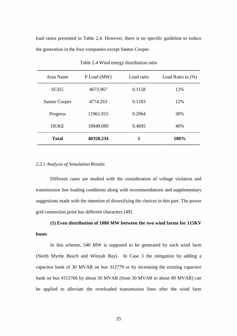
load ratios presented in Table 2.4. However, there is no specific guideline to reduce

the generation in the four companies except Santee Cooper.

Table 2.4 Wind energy distribution ratio

Area Name P Load (MW) Load ratio Load Ratio in (%)

SCEG 4673.967 0.1158 12%

Santee Cooper 4774.263 0.1183 12%

Progress 11961.915 0.2964 30%

DUKE 18948.089 0.4695 46%

Total 40358.234 1 100%

2.2.1 Analysis of Simulation Results

Different cases are studied with the consideration of voltage violation and

transmission line loading conditions along with recommendations and supplementary

suggestions made with the intention of diversifying the choices in this part. The power

grid connection point has different characters [49].

(1) Even distribution of 1080 MW between the two wind farms for 115KV

buses

In this scheme, 540 MW is supposed to be generated by each wind farm

(North Myrtle Beach and Winyah Bay). In Case 3 the mitigation by adding a

capacitor bank of 30 MVAR on bus 312779 or by increasing the existing capacitor

bank on bus #312766 by about 50 MVAR (from 30 MVAR to about 80 MVAR) can

be applied to alleviate the overloaded transmission lines after the wind farm

26

integrated. Case 1, Case 2, Case 4 and Case 5 could not be solved under this

condition.

(2) Uneven distribution of 1080 MW between the two wind farms for

115KV buses

In this scheme, the wind farm located at Winyah Bay has a higher wind power

penetration capacity than the North Myrtle Beach location. By adjusting the amount

of wind power penetrated at each location, Case 2 and Case 3 do not yield any

overloaded transmission lines. The Table 2.5 illustrates the recommended cases

ranked from the best based on the voltage violation and branch power flow.

Table 2.5 Recommended interface buses

Ranking

(High to Low)

Recommended

cases

Interface bus information Injection amount

Bus # Bus Name Bus location Phase I

Phase II

Even

distribution

Uneven

distribution

1 Case 3

312807 '3MYRT BC' Garden City 40 MVA 500 MVA 449.6 MVA

312845 '3WINYAH' Winyah 40 MVA 500 MVA 550.4MVA

2 Case 2

312764 '3DUNES' Dunes 40 MVA N/A 460.4 MVA

312845 '3WINYAH' Winyah 40 MVA N/A 539.6 MVA

2.2.2 Suggestion for Second Stage

The suggestion of the wind energy penetration for the second stage is made in

this part based on the result analysis above. Even though the cost of these suggestions

may be more than the simulation cases above, these schemes are alternatives and

consider because of the system reliability.

27

(1) Using Three 115 KV Interface Buses

The first suggestion uses three 115 KV interface buses instead of two interface

buses, which reduces maximum transmission line loading to 96%. There is no doubt

that the related cost will increase dramatically. However, considering the reliability of

the system when the wind farm is connected to it, this would be an alternative for the

SC grid. In this scenario, 1080 MW wind farm penetrates into Santee Cooper

electrical network at three different 115 KV interface buses. Two of the latter

interface buses are located in North Myrtle beach and the last one in Winyah Bay.

Table 2.6 show a case using three interface buses that has all branches loaded below

96% of their rating in the system.

Table 2.6 Suggested case using three 115kV interface buses

Interface Bus Bus Location

312845 Winyah Bay

312764 Dunes

312807 Myrtle Beach

(2) Using Two 230 KV Interface Buses

The second suggestion uses two 230 kV interfaces buses to bring down the

maximum branch loading to 97.7%. In this situation, the 1080 MW wind energy

enters the Santee Cooper electrical system at two 230 kV interface buses which also

aim to reduce transmission line maximum loading conditions. The result of the power

flow using two 230 kV buses to inject the wind energy into the grid (the two interface

buses are ―312717‖ and ―312719‖) is presented in the South Carolina Offshore Wind

28

farm impact report. Another advantage of using the 230 kV is that the 230 kV

interface buses have a better capacity to absorb more resources and are less likely to

have congested lines; thus less constraints on location of generation reduction within

the four utilities. A total of 16 cases have been successfully tested without any

overloaded lines. In other words, the energy injection at the 230 kV network can

improve the power flow result significantly by reducing lines flow.

2.3 Steady State Analysis Phase III

For the Phase III third scenario, an additional 2 GW of wind farm is expected

to be installed in federal water by the year 2030 after the second stage. The extra wind

power is distributed between five electric utilities: Southern Company, Duke Power

Energy, Progress Energy, Santee Cooper and SCE&G. This is based on the ratio of

their loads based on the summer 2009 power flow. Accordingly, the wind energy

distribution for Phase III (2.08GW) is the following as shown in Table 2.7: 22% for

Duke, 14% for Progress Energy, 5% for Santee Cooper, 6% for SCE&G and 53% for

Southern Company. After reducing the existing generations in the five utilities

accordingly to their load ratios, both 115kV and 230kV transmission systems are

considered to deliver this amount of wind energy.

Different cases are tested using either one voltage rating or a combination of

both voltage ratings for wind energy transmission system. In case penetrating the

whole 2 GW cannot meet the SC system requirement, the limitation of wind energy

can be injected into the SC power system with or without considering the load

29

distribution ratio. In addition, the recommendations for improving the transmission

network are provide to deliver more offshore wind energy.

Table 2.7 Wind energy distribution ratio

Company Percent of 3GW The Wind power(MW)

SCE&G 6% 180

Santee Cooper 5% 150+80

PROGRESS 14% 420

DUKE 22% 660

SOUTHERN 53% 1590

2.3.1 Analysis of Simulation Results

The results of the voltage violations (V<0.94 p.u. or V>1.06 p.u.) and the

transmission lines overloading are discussed below. The orange color represents the

115 kV buses zone and the green color the 230 kV. The simulation cases are divided

where the distribution ratio is followed. The SC 115 kV transmission system is not

able to consume the whole extra 2 GW wind. In order to identify the amount of the

115 kV system wind energy penetration capability, the incremental amount of wind

power injection in the system is tested. It is found that the SC power system

maximum wind energy penetration capacity is about 1191.6 MW for 2009 summer

case, which is accomplished by 442.8 MW at Winyah and 748.8 MW at Dune. Table

2.8 shows the rest interface bus limitation.

30

Table 2.8 System injection limitation

Number of buses in a set 2 buses 3 buses 4 buses 5 buses

Injection capacity of the

original system 1192 MW 1280 MW 1280 MW 1280 MW

Based on two 115 kV buses for Phase I and II (80 + 1000 MW), the third stage

wind injection is using two 230 kV for Phase III (2 GW). For the 230 kV transmission

systems, the results show it has a maximum penetration case with capacity of 2001.6

MW which is accomplished by 720 MW in Santee Cooper network at Perry R bus and

1281.6 MW at Winyah Bay bus. This case doesn’t have any overloaded transmission

lines for the whole 3080MW wind penetration. Table 2.9 shows the rest 230kV

interface buses for offshore wind farm injection. However, the other injection cases

require three new transmission lines (new line# 1, 2 and 3 of Table 18) for the system

to handle the whole 3.08 GW without any overloaded branch.

Table 2.9 List of Santa Cooper’s 230 kV coastal buses

Bus Name Bus location

6WINYAH Winyah

6MYRTLE Myrtle Beach

6PERRY R Georgetown

6CAMPFLD Camp Field

6CHARITY Georgetown

6REDBLUF Myrtle Beach

31

The specific interface buses and the amount of energy consumed at each bus

are listed on Table 2.10.

Table 2.10 Distribution of wind power between interface buses

Bus Name Bus Location Area Wind Turbine Wind Injection

6Perry R Myrtle Beach Santee

Cooper 266 957.6MW

6Winyah Winyah Bay Santee

Cooper 295 1062 MW

Dune Myrtle Beach Santee

Cooper 121 435.6 MW

Winyah Winyah Bay Santee

Cooper 151 534.6 MW

Dune Myrtle Beach Santee

Cooper 12 43.2 MW

Winyah Winyah Bay Santee

Cooper 11 39.6 MW

Total 3080 MW

2.3.2 Suggestion for the Third Stage

(1) Wind Energy Distribution with Reduction Criteria not observed

The idea is not to follow the generation reduction based on the load ratio (the

wind energy distribution criteria). The absorption capacity of the SC power system

can be greatly improved if most of the generators reduction is done within the Santee

Cooper network, specifically at the Winyah Bay generation. In other words, if a large

portion of the wind energy can be consumed by Santee Cooper locally instead of

changing the power flow of a remote area, it will improve the SC system steady stage

performance with the wind farm connection. To successfully implement this idea, the

generation at the power plants in Santee Cooper area should be reduced to their

minimum value primarily. By not following the wind energy distribution criteria,

32

about 2361.6 MW extra wind energy can enter the Santee Cooper network at two 230

kV without a branch overload which is accomplished by 720 MW at 6Perry and

1641.6 MW at Winyah Bay. With this concept, the power system can absorb the

whole 3080 MW without any upgrade for the scenario that utilizes concurrently two

115 kV (1080 MW) and two 230 KV (2 GW) as interface buses. Table 2.11 shows the

critical generators for solving congestion at Winyah Bay when wind energy

penetration.

Table 2.11 Critical generators for congestion at Winyah Bay area

Bus name gP maxP minP gQ maxQ minQ baseS X

1WINY2 21.000 285 285 100 73.96 130 -175 350 0.21

1WINY3 21.000 285 285 100 73.96 130 -175 350 0.21

1WINY4 21.000 285 285 100 73.96 157 -184 350 0.2513

1PEEDEE 21.000 609 682 200 237.1 250 -155 750 0.18

(2) Adding New Transmission Lines (Distribution Criteria follows)

In case the distribution criteria according to load ratio is required among these

five utilities, the improvement of the power system by adding new transmission lines

is mandatory to accommodate the 3080 MW wind energy into the SC power system.

Depending on the interface bus combinations, the number of the new transmission

line required varies. The suggested new transmission lines are listed in Table 2.12.

The study is done by voltage ratings: 115 kV, 230 kV, and a combination of both.

33

Table 2.12 Suggested new transmission lines

Line

#

New transmission line information

From To Circuit# ..upR ..uLpX ..upcX Lim A

MVA

Lim B

MVA

Lim C

MVA

1 311650 312729 2 0.00171 0.02274 0.08939 797 797 1100

2 304632 304654 2 0.03251 0.08671 0.0106 97 97 97

3 312845 312770 10 0.0035 0.0309 0.0043 239 275 275

For SC 115 kV transmission network, adding new transmission lines to the

power system doesn’t improve its injection capability unless more than four interface

buses are put into use. By doubling the capacity of the transmission line connecting

6Peedee to 6Marion (Line# 1 on Table 2.12), the injection limit of the system is

increased to 2080 MW (see Table 2.13 below for more details).

Table 2.13 System injection limit using different set of 115 kV buses

System 3 interface buses 4 interface buses 5 interface buses

Original + 1 New Line 1280 MW 2080 MW 2080 MW

For 230 kV SC transmission system injection, the total amount of 3080 MW

wind energy can enter the Santa Cooper grid at two 230 kV buses without any

overloaded transmission line if the new line 1 and 2 of Table 2.12 are added to the

network. Even though there are three transformers that are loaded at about 105% of

their rating, this is an acceptable loading condition for transformer. However, this

scheme generates under voltage violation at system buses, but it can be fixed by shunt

34

capacitors. The results of the power system with adding new transmission lines and

using two 230 kV buses interface buses in Santa Cooper is included in the SC wind

farm report.

Table 2.14 Cases with new transmission lines

Case # Bus voltage rating

115 KV bus Number 230 KV Bus Number

1 312845 312807 312719 312717

2 312845 312807 312719 312726

2.3.3 Testing of 2009 Light Load Base Case

Since the only light load base case power flow available is for 2009, 3.08 GW

of wind energy is injected into the power grid to check its penetration capability

during off peak hours. However, the result of the simulation shows that the system

can only take about 2150 MW without overloading any branch. The presence of wind

energy in the power network improves tremendously over the overvoltage aspect of

the 2009 light load case by reducing the number of bus overvoltage violations to the

third of its original values. Table 2.15 displays the specific information related to the

voltage violations in the original and the system with wind energy, which uses two

230 kV interface buses.

35

Table 2.15 Voltage violations at light load

System

# of buses with

voltage below

0.94 p.u.

# of buses with

voltage above

1.06 p.u.

# of buses with

voltage above

1.08 p.u.

Lowest

voltage

(p.u.)

Highest

voltage

(p.u.)

Original system (2009

Light Load) only 11 buses 262 buses 18 buses 0.916086 1.15422

Original system with 2150

MW of wind energy 11 buses 76 buses 9 buses 0.916777 1.13879

The evaluation of the results shows that if the wind energy distribution criteria

based on load ratios is followed, the power system cannot handle the whole 3.08 GW.

At 115 kV voltage rating, the power grid has an injection limit of about 1190 MW and

2000 MW at 230 kV (using two buses at a time). To improve the injection capacity of

the network to accommodate the 3.08 GW, two approaches are taken. The first one is

not to follow the wind energy distribution criteria, i.e. a large amount of the energy

are consumed by Santee Cooper’s load. However, this solution may not be feasible. A

successful case to use two 115 kV buses and two 230 kV buses for interfacing the

wind farms is presented in Table 2.16. The second method adds new lines to increase

the transmission capability of the power system. There are two scenarios in which the

power grid can successfully absorb the 3.08 GW with a minimum number of new

lines. The first scenario, which requires 2 new lines (lines 1 and 2 on Table 2.16), uses

two 230 kV buses as wind energy interface buses. The second scenario, which

requires 3 new lines (all the new lines on Table 2.16), use two 115 kV and two 230

kV buses as interfaces. In conclusion, the study of the 2009 Light Load base case

shows that the wind energy reduces the voltage violation.

36

Table 2.16 Recommended interface buses for injecting 3080 M

Interface bus

voltage rating Interface bus# Bus Name

Original power

system

Power system with

improved Transmission

capability

Scenario I scenario II

115 kV

312764 Dune 435.6 + 43.2 MW N/A N/A

312807 3MYRT BC N/A 540 MW N/A

312845 Winyah 534.6 + 39.6 MW 540 MW N/A

230 kV

312717 6Perry R 957.6 MW N/A N/A

312719 6Winyah 1062 MW 1000 MW 1540 MW

312726 6REDBLUF N/A 1000 MW 1540 MW

New

transmission

lines

Line 1: 6PEEDEE to 6Mariom N/A Yes Yes

Line 2: 3MARION1 to

3DILLN T N/A Yes Yes

Line 3: 3WINYAH to 3GTWN

s N/A Yes No

Wind energy distributed based on the 5 utilities

load ratio No Yes Yes

Total wind energy injection 3080 MW 3080 MW 3080 MW

36

CHAPTER THREE

OFFSHORE WIND FARM SWITCHING TRANSIENT STUDY

The next chapters focus on the impact of the switching transient of the

offshore wind farm on the SC power system. Recently, a switching transient or fault

associated with wind farm failures has been reported [18]. The transient overvoltage

and inrush current may damage equipment and disturb power delivery as well as

affect voltage stability [50]. The resulting equipment maintenance and repair cost are

higher for offshore wind farm than for onshore ones. Thus, researchers have

investigated in electromagnetic transient in offshore wind farms, with relevant studies

have been carried out on such wind farms such as, which is based on fixed speed

induction generators. A switching transient impact study requires a detailed model of

wind farms. However, it is difficult to model each generator because of simulation

time constraints. Using wind farms consisting of large numbers of relatively small,

identical generating units makes comparison possible. One of the most frequently

used equivalent models for wind farms is based on aggregation of the wind generator

units. This chapter presents a DFIG based wind farm equivalent model is presented

for switching transient operation analysis. After the equivalent model results are

verified with a detailed model, several switching operations are designed to

investigate their impact on the system.

37

3.1 The Equivalent Wind Farm Model

3.1.1 Offshore Wind Farm Collecting Grid for Transient Study

Generalized offshore wind farm grids consist of a large number of identical

wind generators, step-up transformers, submarine cables and offshore substations as

shown in Figure 3.1. The DFIG model used in this chapter is available at PSCAD’s

website [36] with the machine parameters listed in Table 1. Each DFIG’s capacity is

0.9MW with an output voltage of 0.69kV. This model uses a Synchronized Pulse-

Width Modulation (SPWM) converter at the grid side to ensure the constant direct

voltage resource for the rotor side converter, which is a Current Reference Pulse-

Width Modulation (CRPWM) converter. The stator Flux Oriented Reference Control

(FOC) decouples the rotor current to control the DFIG output power and frequency

[51]. For the step-up transformer, the DFIG output voltage is raised from 0.69kV to

34.5kV. Saturation is considered, but winding losses and copper losses are neglected

in the simulation. All units are connected in parallel to the collecting bus. Wind power

would then be transmitted to the offshore substation, which steps up the voltage from

34.5kV to a 115kV transmission system level before its connection to the interface

bus onshore. The submarine cables are simulated as pi-section in this model.

3.1.2 Concept Equivalent Modeling for Transient Study

The identical wind generators are connected in parallel in each column, and all

columns are connected to the offshore substation. The concept of the equivalent wind

generator and its step-up transformer are represented in Equation (3-1) and Equation

(3-2).

38

34.5/115KV

4MVA0.69KV

3.6MVA

0.69/34.5KV

4MVADFIG unit

Wind farm

Row1

0.69KV

0.9MVA

DFIG unit0.69/34.5KV

1MVA

0.69KV

0.9MVA


1MVA

0.69KV

0.9MVA


1MVA

0.69KV

0.9MVA


1MVA

34.5/115KV

4MVA

Figure 3.1 Wind farm configuration and aggregation

drealTdrealgerealTerealg XX

nXX ________

1 ······················ (3-1)

dpuTdpug

base

base

base

baseepuTepug XX

S

V

nS

VXX

n________

11 ····· (3-2)

where,

erealgX __ , and erealTX __ represent the real values of the equivalent wind generator

impedance and the transformer impedance, respectively.

drealgX __ , and drealTX __ represent the real values of detailed wind generator

impedance and detailed the transformer impedance, respectively;

39

epugX __ , and epuTX __ represent the per unit values of equivalent wind generators and

transformers, respectively;

dpugX __ , and dpuTX __ represent the per unit values of detailed wind generators and

transformers, respectively;

Vbase represents the rated voltages of individual DFIG.

Sbase represents the rated capacity of individual DFIG.

The equivalence of the n paralleled generator units has the same machine per

unit as an individual one, but the capacity base increases by n times, as shown in

Table 3.1. The machine converter configuration of the equivalent model is the same

as the individual model. However, the control parameters need to be changed, this

procedure is detailed in the next section.

Table 3.1 DFIG detailed model and equivalent model

Parameter (p.u.) Equivalent One DFIG

MVA 9.0n 0.9

statorV 0.69 0.69

statorR 0.0054 0.0054

lsL 0.1 0.1

rotorR 0.00607 0.00607

lrL 0.11 0.11

mL 4.5 4.5

windv 12 12

3.1.3 Equivalent Procedure

Based on the equivalent concept, the wind generator and its step-up

transformer equivalent modeling is accomplished through the following steps:

40

Step 1 Using individual DFIG machine parameters (the rotor and stator

resistance and the reactance) for the equivalent model;

Step 2 Increasing the rating of the individual DFIG by n times for the

equivalent model;

Step 3 Calculating the equivalent machine steady state values based on the

given machine parameters using the equations (3-3)-(3-9) and using

them as reference value for the rotor side control.

Step 4 Adjusting the capacitor and its charging resource to provide smooth

DC voltage for the converter on the rotor side as shown in Figure 3.2;

Step 5 Selecting the appropriate rating for the transformer on the grid side

converter based on the rotor voltage calculated;

Step 6 Tuning the PI controller’s parameter for both the rotor side current

loop and grid side voltage loop for optimal transient study.

ss

ss

V

PI

cos3 ····························································· (3-3)

r

Slmrr

L

ILI

······························································ (3-4)

ssss jVRI 1 ······················································· (3-5)

'

1 rrrrr EsjVRI ··············································· (3-6)

'

11 prlmssss EILjVLjRI ····································· (3-7)

41

rr

r

rs

r

mr Vjs

L

RI

L

LR

1 ·········································· (3-8)

sr

m

rscss V

L

LjLjRI 11

··········································· (3-9)

Induction Generator

Gearbox Rotor Converter Grid Converter

Figure 3.2 Control blocks for DFIG

3.1.4 Equivalent Model Verification

Because of the limitation of the PSCAD, the maximum four DFIG detailed

models (0.9 MW each) can be run to verify the results obtained from the equivalent

model (3.6 MW) results as shown in Figure 3.3 - Figure 3.5. The generators start from

speed control until t=0.5 sec when the torque control is engaged. The active output

power of the two models is shown in Figure 3.3. The steady state results from 0 sec to

3 sec exhibit negligible differences between the two models. The load is switched on

at the system interface bus for both models when t=3 sec phase A voltage achieves

zero crossing. When the load is switched on, the overshoot of output power is

followed by a distortion, the transient of which lasts for 2 sec before arriving at a new

steady state. The maximum error between the two models at active power is 8.3% as

shown in Table 3.2. This model is suitable for studying switching transients, but it

will require further refinement if a stability analysis is involved.

42

Table 3.2 Comparison of two models

— Voltage Current Active

Power

Max Error % 0.29% 8.71% 8.3%

Figure 3.3 The comparison of active power outputs between two models

The phase to phase voltage at the wind farm collection bus during load

switching has a very small transient as shown in Figure 3.4. The error between the

two models, which is shown in green, is less than 0.29% as shown in Table 3.2.

The current of wind farm experiences overshoot before arriving to steady state

as shown in Figure 3.5 and the maximum error between the two models is 8.71% as

illustrated in Table 3.2.

0 1 2 3 4 5 6 7 8-2

-1

0

1

2

3

4

Time(s)

The O

utp

ut

Pow

er(

MW

)

The active power output

Detailed model

Equivalent model

Error(transient within10%)

43

Figure 3.4 Interface bus voltage comparison

Figure 3.5 Interface bus current comparison

2.95 3 3.05-30

-20

-10

0

10

20

30

Time(s)

Voltage a

t in

terf

ace b

us(K

V)

The interface bus voltage compare

Equivalent modelDetailed model

3 3.1 3.2 3.3 3.4 3.5

-0.2

-0.1

0

0.1

0.2

0.3

Time(s)

Lin

e t

o lin

e c

urr

ent(

KA

)

The interface current(KA)

Detailed model

Equivalent model

44

3.2 Wind Farm Switching Transient Impact on Power System

3.2.1 40MW Wind Farm Integrated SC System Units

Using the method detailed in the previous section, a 40MW equivalent wind

farm is established and connected to South Carolina Thevenin’s equivalent

impedance. Wind power is generated and delivered to the offshore substation before

its integration into the system as shown in Figure 3.6.

Generator

Generator

Converter

&Control

Grid

Converter

&Control

Gab

cSabc

40MW DFIG

Equivalent0.69/34.5kV 34.5/115kV SC System

Figure 3.6 40MW equivalent wind farm integration

The steady state voltage and current at wind farm output bus are shown in

Figure 3.7 and Figure 3.8.

Figure 3.7 40MW equivalent wind farm output voltage

The w ind turbine output voltage(KV)

Time... 2.1000 2.1100 2.1200 2.1300 2.1400 2.1500 2.1600 2.1700 2.1800 2.1900 ...

...

...

-40

-20

0

20

40

kV

Vs1

45

Figure 3.8 Current output of 40MW equivalent wind farm

The DFIG converter distortion can be observed in the wind farm output

voltage and current. The current output of the equivalent machine is analyzed using

FFT. It can be observed that 5th, 7th, and 11th harmonics are present with their Total

Harmonic Distortion (THD) being 0.794%, which is less than 1% of the fundamental

frequency as shown in Table 3.3.

Table 3.3 Harmonic components in the wind farm current

Harmonic 5th Harmonic 7th Harmonic 11th

base

h

I

I 0.3% 0.6% 0.425%

The power output of the equivalent wind farm with a unity power factor is

shown in Figure 3.9. The output power of the DFIG can be adjusted through the wind

speed and the slip of each generator.

The w ind turbine output current

Time(s) 2.100 2.110 2.120 2.130 2.140 2.150 2.160 2.170 2.180 2.190 ...

...

...

-50

-40

-30

-20

-10

0

10

20

30

40

50

kA

Iabc

46

Figure 3.9 Power output of 40MW equivalent wind farm

3.2.2 Cable Energizing in Wind Farm Equivalent

Cable energizing is frequently operated inside wind farms. After the DFIGs

are started and synchronized, they are then switched to the system and wind power is

generated after the cable is charged. As seen in Figure 3.10, the cable is switched at

t=3sec. at which time the offshore substation bus voltage of phase A experiences a

voltage dip when the cable is switched on, as shown in Figure 3.11. The simulation

results indicated that the more paralleled cables that are switched on, the larger the

voltage decrease at the substation bus.

SC System

DFIG 3.6MW 0.69/34.5kV

SubmarineCable

34.5/115kV

Offshore Substation

Figure 3.10 Cable energizing wind farm

Wind turbine output pow er(MW)

TIme(... 0.00 0.10 0.20 0.30 0.40 0.50 0.60 0.70 0.80 0.90 1.00 ...

...

...

0.0

5.0

10.0

15.0

20.0

25.0

30.0

35.0

40.0

P(M

W)

Pg

47

Figure 3.11 Voltage at the substation at cable switching

3.2.3 Three-Phase Fault at Different Locations in a Wind Farm

The three-phase fault at various locations in wind farm has different impacts

on the system. In this section, it is assumed that the three-phase fault occurs at the

DFIG unit output bus (location A), the substation bus (location B), and the system

interface bus (location C) as shown in Figure 3.12. All the faults occur at t=3sec,

lasting for 0.15s before being cleared.

34.5/115kV0.69/34.5kV

Generator

Generator

Converter&

Control

Grid

Converter&

Control

GabcSabc

40MW DFIG

Equivalent

SC System

Figure 3.12 The three-phase fault in a wind farm

48

The fault current at the various locations are shown in Table 3.4. The

maximum fault current occurs at the interface bus, where the value reaches 68 kA.

The minimum fault current, which occurs at DFIG bus, is 14.5 kA.

Table 3.4 Comparison of three-phase fault at different locations

Fault (kA) (MW) /Overshoot (RMS) /Overshoot

Location A 14.5 45.2/31.03% 0.98/-2%

Location B 19 64.5/86.96% 1.01/1%

Location C 68 71.25/106.52% 1.07/7%

The fault current injected by the wind farm reaches approximately 2.5 times of

rated value when the three-phase fault occurs. When the fault is cleared, the largest

recovery current injected from the wind farm reaches approximately 4 times the rated

value as shown in Figure 3.13.

Figure 3.13 Three-phase fault currents at different locations

The fault currents injected by the wind generators are small compared to the

one from grid as shown in Figure 3.14.

2.95 3 3.05 3.1 3.15 3.2 3.25 3.3 3.35 3.4 3.45-4

-3

-2

-1

0

1

2

3

4

5The fault current contributed by wind farm

Time(s)

If_

_w

f

Fault at DFIG bus

Fault at substation bus

Fault at system bus

49

Figure 3.14 Wind farm injected fault current at different location fault

The wind farm output power disturbance due to the fault at various locations is

shown in Figure 3.15. The power is interrupted during faults, and generators

experience fluctuation before the power reaches its steady state value. The maximum

power output fluctuation of the wind farm occurs when a fault is located at the system

interface bus, the overshoot of which reaches 71.25 MW. The minimum power output

fluctuation occurs when a fault is located at the DFIG output bus.

Figure 3.15 Three-phase fault power at different locations

2.95 3 3.05 3.1 3.15 3.2-40

-20

0

20

40

60

80

Time(s)

Ifsyste

m

Fault current contributed by system

Fault at DFIG bus

Fault at substation bus

Fault at grid bus

0 1 2 3 4 5 6-20

0

20

40

60

80

Time(s)

P(M

W)

The Output Power of Wind Farm

Output Bus

Substation Bus

System Bus

50

The voltage drop due to a fault at different locations in the wind farm is shown

in Figure 3.16, a voltage dip during a fault can be affected by the capacitor bank in the

DFIG converter. After the fault is cleared, the voltage reaches its steady state. The

maximum overvoltage of 7% occurs when a fault is located at the system interface

bus while the minimum happens when a fault is located at the DFIG output bus.

Figure 3.16 Three-phase fault voltage RMS at different locations

Figure 3.17 illustrates the recovery voltage at the offshore substation bus when

fault is cleared at t=3.15sec at three locations. The max transient recovery voltage

distortion occurs when a fault is located at the system interface bus while the

minimum transient happens when a fault is at the DFIG output bus.

2 2.5 3 3.5 4 4.50

0.2

0.4

0.6

0.8

1

1.2

1.4

Time(s)

Vrm

s

The voltage dip when fault happens

Fault at WF output bus

Fault at Substation bus

Fault at Interface bus

51

Figure 3.17 Recovery voltage after the faults have cleared

3.3 Conclusions

An offshore wind farm switching transient would impacts the injection

system. The simulation of this switching transient requires appropriate models of

wind farm equipment. The one used here indicated that load switching in the

connected system causes a dynamic power fluctuation in wind farms. In addition,

cable energizing causes a voltage dip in the connected bus: the more paralleled cables

charged at the same time, the greater this voltage dip. Different fault locations in wind

farm cause disturbances in the system.

3.12 3.14 3.16 3.18 3.2 3.22 3.24 3.26-40

-30

-20

-10

0

10

20

30

40

Time(s)

Voltage(k

V)

The Recovery Voltage at the Substation Bus(kV)

Fault at WF output Bus

Fault at Substation Bus

Fault at System Interface

52

CHAPTER FOUR

SWITCHING TRANSIENT IMPACT OF OFFSHORE WIND FARM ON POWER

SYSTEM

Given their frequency in a system, switching operations can be a source of

transient overvoltage or inrush current, both of which cause stress on the insulation

material of the equipment, malfunction of the protection, shedding of the load, or

damage to the equipment, resulting in the instability in the system [52]. They also

affect wind farm operation because of the switching transient. Thus, the impact of this

switching transient on power systems with offshore wind farms is important to

investigate. Large power system electromagnetic transient studies require detailed

modeling of specific parts, and the remaining parts of the system have to be reduced

as equivalent impedance [53].

Research focusing on the switching transient impact of an offshore wind farm

on the system is shown in [54]. The first consideration needing to be addressed for a

study of the effect of a transmission system switching transient for a large scale

offshore wind farm is whether to use appropriate equivalent models for each

component in the power system [55][56][57][58]. As shown in Figure 4.1, a

configuration and aggregation of an offshore wind farm consists of identical DFIGs;

this type of aggregation DFIG model should be available before studying the transient

impact.

After modeling, the switching transient analysis determines the solutions for

ordinary differential equations under switching operating conditions. They can be

solved either using an analogue or a digital simulator [52]. Analogue simulation is

53

appropriate for simple systems. For electrical power system whose variables are

continuous, suitable methods have to be chosen to solve the differential equations at

discrete points. As mentioned in Chapter One, numerical integration and difference

equations are two methods for converting a continuous system into a discrete one to

solve differential equations. Software based on the discrete algorithm includes EMTP,

EMTDC/PSCAD, among others.

The research reported in this chapter continues the investigation of the

influence of switching transient offshore wind farms on the SC power system. In this

chapter, both offshore wind farms (OWF) and the SC power systems are modeled in

detail and implemented. In addition, various different system modeling are studied to

investigate the switching transient impact of OWF connected power systems. After

establishing the system model, different scenarios including capacitor bank switching,

the three-phase fault and its clearance are examined. In order to better observe the

switching transient impact of offshore wind farms on the SC power system, the results

are compared with those obtained from system supplied by a comparable

conventional generator. The transient frequency is analyzed in frequency domain.

4.1 System Description

4.1.1 Offshore Wind Farm Equivalent Model

Since offshore wind farms consist of large numbers of relatively small,

identical generating units, a GE 3.6 MW wind turbine for example, it is possible to

build equivalent models without losing accuracy. One of the ways to establish

equivalent models for wind farms is by aggregating wind generator units. This section

54

adopts the OWFs equivalent model developed and verified using a 3.6MW model in

previous chapter, meaning a 40MW DFIG based wind farm equivalent model is used

here for switching transient operation analysis. Several switching operations are

considered to investigate their impact on the system.

4.1.2 South Carolina Reduced System

The first system to be simulated focuses on the surrounding area of two OWFs

surrounding areas with the remaining connected as Thevenin equivalent impedance

and infinite voltage sources. The OWFs are injected into the system through selected

interface buses Dunes as (D) and Winyah Bay as (W) based on the previous study as

shown in Figure 4.2. This reduced South Carolina power system is composed of

approximately 61 buses and 21 plants with a total capacity of 2064.7MW.

Table 4.1 SC reduced system data

System Information Numbers

System Generation 2064.7MW/1773.5MVar

Constant Load 1903.9MW/569.5MVar

Bus Number 61

Plants Number 21

Fixed Shunt 16

Switched Shunt 10

Load Number 37

Branch Number 86

Transformer Number 31

The system data are listed in Table 4.1, and the wind farm penetration level is:

55

%87.3%100MW7.2064

MW80 ············································· (4-1)

4.1.3 South Carolina intentional islanded power system

Intentional islanding [59][60] is the purposeful separation of the utility system

during a specific operation mode to create power "islands". Previously, due to the

large capacity of the connected system compared to the OWF, the penetration level

was 3.87%, and the transient could not be observed clearly. In order to better

investigate the impact of an offshore wind farm switching transient, an intentional

islanded system is created around OWFs connecting points to reduce the system size

further. The system is assumed to operate under a light loading condition in which

large generators are operating at minimum capacity and the large loads are

disconnected from the system. The system size reduced using PSSE based on the

previous section is listed in Table 4. 2. The intentional islanded system size was

decreased to 46 buses with the capacity of 602MW. The system data are listed in

Table 4.2.

Table 4.2 Intentional islanded system data

System Information Numbers

System Generation 602.1MW

Constant Load 595.6MW

Bus Number 46

Plants Number 10

Fixed Shunt 16

Switched Shunt 10

Load Number 8

Branch Number 70

Transformer Number 19

56

34.5/115KV

3.6MVA

Wind Farm

Row1

0.69 kV

4×0.9 MVA

DFIG Unit

0.69/34.5 kV

0.9 MVA

34.5/115 kV

3.6 MVA

0.69KV

40MVA0.69/34.5KV

40MVA

DFIG Equivalent

34.5/115KV

40MVA

Wind Farm

Row2

DFIG Unit

0.69 kV

3.6 MVA

0.69/34.5KV

3.6MVA

0.69 kV

4×0.9 MVA

0.69/34.5 kV

0.9 MVA

34.5/115 kV

3.6 MVA

0.69 kV

3.6 MVA

0.69/34.5KV

3.6MVA

Figure 4.1 Wind farm configuration and aggregation

The penetration level is increased to:

%29.13%100MW1.602

MW80 ············································· (4-2)

The system diagram in PSSE is shown in Figure 4.2. The OWFs are injected

into the system through selected interface buses Dunes (D) and in Winyah Bay (W).

57

Switching operation and faults are placed in the system, and the results are compared

with those of a comparable system supplied by conventional generation.

Figure 4.2 Intentional islanded zone

4.2 Computer Modeling Procedure

4.2.1 South Carolina Reduced System

Usually the system data are given as PSSE sav files or raw files, both of which

need to be translated into PSCAD before connecting the OWFs. After reducing the

systems in PSSE based on the different operation modes, the network data are

translated into PSCAD by ETRAN as shown in Figure 4.3. The 40MW equivalent

OWF model is connected at the selected interface bus of the system.

58

Power Flow

PSSE File

(.sav or .raw)

Equivalent

SystemETRAN

PSCAD

System Data

(.psc)

Equivalent DFIG

Wind Farm

Simulation

System

Figure 4.3 System modeling in PSCAD

Based on the system modeled in PSCAD, the switching scenarios, capacitor

bank switching and three-phase fault analysis, are carried out to simulate various

operations in the system with offshore wind farms. Since the system to be reduced is

too far away to affect the frequency performance of the highlighted small scale OWF-

surrounded system, for the purpose of this case, non-frequency dependent network

equivalents are used. After selecting a specific zone, the original system is modeled as

an equivalent one in PSSE according to the interface requirements.

4.2.2 Equivalent PSCAD Model Imported From PSSE

Case 0: The original data are in PSSE31 Format. Using the 2007 series SERC

LTSG power flow model of the 2013 summer peak data which includes 50988 buses,

6009 power plants, and machines 7072 machines without wind machines included.

Case 1: The four areas include CPLE, CPLW, Duke, SCE&G, and Santee

Cooper; a voltage level above 110kV; a generator above 100MW retained from the

equivalent system; a retain area boundary bus; retain control buses;

59

Case 2: Six interface buses in Zone 342 and 1375; a voltage level above

110kV; a generator above 100MW retained from the equivalent system; retained area

boundary buses; retain control buses.

The cases data are listed in Table 4.3

Table 4.3 Equivalent cases summaries

Bus

Number

Plant

Number

Fixed

Shunts Loads Branches Transformer

Case 0 50988 6008 3306 31078 67195 19475

Case 1 684 185 203 565 1942 229

Case 2 165 123 101 114 1129 61

As shown in Figure 4.4, Etran bridges the gap between the phasor-based load

flow and the stability simulation tools and electromagnetic transient (EMT) tools. It

solves the steady state phasor equations and uses this information to initialize a

PSCAD/EMTDC circuit as well as to form network equivalents to reduce the network

so that it is suitable for transient analysis.

PSSE 31

DATAEtran PSCAD

Figure 4.4 Data imported from PSSE to PSCAD

The steady state solution in PSCAD/EMTDC is based on the solution of

instantaneous differential equations, whereas the solution in PSS/E or load flow

programs is based on phasor-based complex variable calculations at the fundamental

60

frequency. The load flow information is used by ETRAN to initialize the circuit in

PSCAD/EMTDC.

4.2.3 South Carolina Intentional Islanded Power System

The procedure for modeling the intentional islanded zone in PSCAD is listed

below:

Step 1 Determine the system to be islanded. For this research, this system is

the east zone of the SC power system;

Step 2 Determine the power flow at the tie lines and the connection buses in

the zone into which the OWFs are injected. The power flow on the tie

line between the zones is listed in Figure 4.5;

Figure 4.5 Intentional islanded zone and tie lines

61

Step 3 Use the interface bus voltage as the voltage source and the power

flow at tie line as the equivalent generator output capacity as shown

in Figure 4.6.

tielinetinline jQP

equivalentZ

Figure 4.6 Equivalent for the rest system

Now the impedance can be calculated using Equation (3),

)(

2

tielinetieline

tielinetieline

jQP

VZ ·················································· (4-3)

Step 4 The system outside the SC east zone power system is an equivalent as

voltage resource and impedance as shown in Figure 4.7;

Step 5 Keep the generator above a 200MW run as the minimum output and

reduce the same amount of load;

Step 6 Run PSSE until the power flow converges;

Step 7 Load the converted PSSE raw file in ETRAN; then convert the PSSE

file into a PSCAD file for the electromagnetic transient study; and

Step 8 After the system is converted into PSCAD, the OWFs equivalent

model can be connected to the interface bus, and the simulation cases

applied to investigate the switching transient impact.

62

4.3 Case Simulation

This section analyses the simulation results from the reduced South Carolina

power system and the corresponding intentional islanded power system modeled with

connections of the offshore wind farm equivalent system. Switching operations

including capacitor bank switching, three-phase fault application and its clearance,

and the disconnection of the wind farm from the system will be analyzed and the

results are discussed.

4.3.1 Capacitor Bank Switching and the Three-Phase Fault

Capacitor bank switching frequently occurs in power systems for voltage

regulation and power factor improvement. In the first case, the 30MW capacitor bank

located at the OWFs neighboring bus P is switched on at t=0.2 sec. The transient

voltage waveform at the wind farm interface bus D obtained as seen in Figure 4.7

indicate that the switching has little impact on the OWF bus.

Figure 4.7 Voltage wave of the capacitor switching

Assume that at t=0.2 sec the three-phase fault occurs at bus P and lasts for

0.05s before it is cleared itself. The voltage transient at the wind farm interface bus is

0.18 0.185 0.19 0.195 0.2 0.205 0.21 0.215 0.22 -150 -100

-50

0

50

100

150

Time (s)

KV

63

shown in Figure 4.8. The voltage deceases by 40% during the fault and the transient

recovery voltage overshoots by 20%.

Figure 4.8 Voltage wave of three-phase fault

4.3.2 Offshore Wind Farm Disconnection

The wind farm is disconnected from the system when the wind is blowing too

strongly. This section analyzes the simulation conducted to investigate the transient

caused by the disconnection of the OWF from the SC power system. It is assumed

that the wind farm at Dune (bus D) would be disconnected at t=0.2 sec. The voltage

transient at the wind farm interface bus is illustrated in Figure 4.9.

Figure 4.9 Voltage wave of OWF disconnection

0.196 0.198 0.2 0.202 0.204 0.206 0.208 -100 -80 -60 -40 -20

0 20 40 60 80

100

Time(s)

kV

0.2

0.21 0.22 0.23 0.24 0.25 0.26 0.27 0.28 -150

-100

-50

0

50

100

150

Time (s)

KV

64

As shown in Figure 4.9, due to the low penetration, the disconnection of the

OWF has a negligible effect on the South Carolina equivalent system.

For the islanded system surrounding a small region of the OWFs, a 30MW

capacitor bank located at the OWFs neighboring bus P as shown in Figure 4.2 is

switched on at t=0.2 sec. The transient current waveform for the capacitor bank

obtained is shown in Figure 4.10. The blue plot represents the system supplied by the

same amount of conventional generation at the OWFs interface bus, and the red plot,

the DFIG equivalent wind farm supplied system. As seen from Figure 4.10, both

transients die out within a half cycle. However, a harmonic is present in the capacitor

bank inrush current in the system supplied by the OWFs during steady state.

Figure 4.10 Capacitor bank inrush current at bus P

The frequency analysis for the capacitor bank current is given in Figure 4.11.

The main harmonic component is the 19th order and the amount is approximately 3%

in comparison with the fundamental frequency component. As seen in Figure 4.11,

the system supplied by the OWFs has more frequency components than the system

supplied by conventional generator during the capacitor switching transient.

1 1.01 1.02 1.03 1.04 1.05 -0.5 -0.4 -0.3 -0.2 -0.1

0 0.1 0.2 0.3 0.4

Time (s)

kA

Conventional Generator

OWF Generators

65

Figure 4.11 Frequency analysis of the capacitor inrush current at bus P

4.3.3 Three-Phase Fault and its Clearance in the Intentional Islanded System

A three-phase fault occurs at bus P at t=0.6 sec, lasting for 0.05 sec before it

clears itself. Figure 4.12 and Figure 4.13 show the transient recovery voltage of the

wind farm interface bus when the fault is cleared.

Figure 4.12 Transient recovery voltage of the OWFs supplied system

Figure 4.12 shows the system supplied by the OWFs, and Figure 4.13 for the

system with the same amount of conventional generation at the OWFs interface bus.

Both transient die out within one cycle. However, the system supplied by

50 0

0.645 0.65

0.655 0.66

0.665 0.67

0.675 0.68

0.685 0.69

0.695 -200

-150

-100

-50

100

150

200

Time(s)

kVV

0 120

240

360

480

600

720

840

960

1080

1200

1320

1440

1560

1680

1800

1920

0 0.002 0.004 0.006 0.008 0.01

0.012 0.014 0.016 0.018 0.02

Frequency (Hz)

OWF Generation Conventional Generation

kV

2000

66

conventional generators exhibits a worse transient than the OWFs supplied system

with greater overvoltage and a longer transient period.

Figure 4.13 Transient recovery voltage of the conventional generator system

For the frequency analysis shown in Figure 4.14, the system supplied with

conventional generator exhibits a higher frequency component other than the system

supplied by the OWFs because the DFIG grid side converter contributes to the system

transient voltage.

Figure 4.14 Frequency analysis of the transient recovery voltage

0 200

400

600

800

1000 1200 1400 1600 1800 2000 0

0.664

1.328

1.992

2.656

3.32

3.984

4.648

5.312

5.976

6.64

Bus B Voltage when 3 phase fault frequency analysis

Frequency (Hz)

kV

0.645

0.65 0.655

0.66 0.665

0.67 0.675

0.68 0.685

0.69 0.695

-200

-150

-100

-50

0

50

100

150

200

Time(s)

kV

67

4.4 Conclusions and Future Work

Based on the study reported in this chapter, it can be concluded that:

1. For the South Carolina power system with surrounding area as equivalent

systems, 80MW offshore wind farm does not affect system switching

transient significantly because of small capacity.

2. The steady state analysis of the islanded system indicates that the DFIG

wind farm inject the 19th harmonic into the system.

3. During the transient period (within 1 cycle) for the light load with the

minimum generation and the intended islanding system, the doubly fed

induction generators based offshore wind farms exhibit less transient

compared to the regular generators.

4. For future work, the wind farm capacity should be increased by another

1GW, and the corresponding studies conducted to determine the effect of

this increase.

.

68

CHAPTER FIVE

FREQUENCY DOMAIN ANALYSIS OF THE IMPACT OF THE OFFSHORE

WIND FARM SWITCHING TRANSIENT

5.1 Introduction

For the transient analysis of large systems with wind farms integrated using a

digital simulator, the detailed data about the system has to be available before the

simulation. While the time domain simulation can provide the switching transient

impact of the offshore wind farm on the system by modeling it in such software as

PSCAD or EMPT, in some case when data from the entire system are not available,

an equivalent system model has to be built or as an alternative, the appropriate system

equivalent models have to be provided. However, for practical engineering projects

studying the impact of the wind farm transient impact on the system, it’s difficult to

acquire the detailed system data and build the entire system in transient software for

the analysis. Even if the information is ready, after building the system for the

simulation, PSCAD or EMTP may not be able to obtain results because of the

simulation time. Thus, system side equivalent models for transient analysis have to be

developed to represent the performance of specific aspects of the system. However,

these equivalent systems are also based on the detailed system data.

In order to address this problem, a frequency domain impedance matrix based

offshore wind farm transient study is presented in this chapter. The goal of this

method is to find a mathematic process for determining how DFIG-based offshore

wind farm affects system switching transient. Frequency domain impedance modeling

for the DFIG is critical for this research. Unlike the studies conducted in time domain

69

simulation, a frequency domain impedance model is developed for Type 3 wind farm

in DQ reference frame by transforming the machine control at DQ reference. The

converter and control are also included in the impedance model. The nonlinear system

is linearized by modeling the machine and control at DQ reference frequency.

Decoupled at the rotor and stator side at the same time, quantities are difficult to be

control separately so it is not easy to derive the explicit expression for impedance

model. The feed forward decoupled controllers are implemented both at the grid side

converter control and the machine side converter control. The DFIG transfer function

is derived after applying the two controllers. The equivalent frequency domain matrix

for the DFIG is tested both under the steady state and transient scenarios with the

results being compared with the same scenarios in PSCAD.

Researches focusing on the modeling of the impedance model for the DFIG

are applied in papers [61][62][63] for Sub-synchronous Resonance (SSR), the

induction machine impedance model being derived in the dq-axis. However, the

control and PWM are not derived but rather expressed in equivalent circuits. In the

paper [64], the small signal method is applied to derive the impedance matrix of the

DFIG.

The first part of this chapter discusses the derivation of the DFIG model in the

frequency domain. It is divided into two parts since DFIG has two PWM converters,

one at the grid side and one at the rotor side. After the derivation, both parts of the

impedance matrix are combined as the steady state and transient response of the

frequency domain DFIG model and are verified with the PSCAD results. Conclusions

are given based on the simulation results.

70

In this part of the dissertation, the following notations are used in the

equations for the stator and rotor circuits:

Vas,Vbs,Vcs instantaneous stator phase to neutral voltages

ias,ibs,ics instantaneous stator current in phase a,b,c

Var,Vbr,Vcr instantaneous rotor phase to neutral voltages

iar,ibr,icr instantaneous rotor current in phase a, b, c

Rr, Rs rotor winding resistance and armature resistance per phase

λsa, λsb, λsc stator winding flux

λra, λrb, λrc rotor winding flux

LAA, LBB, LCC self-inductance of stator windings

LAB, LBA, LBC, LCB, LAC, LCA mutual inductance between stator windings

Laa, Lbb, Lcc self-inductance of rotor windings

Lab, Lab, Lbc, Lcb, Lac, Lca mutual inductance between rotor windings

LAa, LAb, LAc, LBa, LBc, LBc ,LCa, LCb, LCc mutual inductance between rotor and stator

windings

p differential operator d/dt

5.2 The Approach

A frequency domain DFIG impedance model is imperative in order to apply

the frequency domain analysis for determining the switching transient impact on the

system. The goal of this approach is to determine the relationship between the output

voltages of DFIG Vabc and the current from grid converter Isabc and the current from

the machine side Igabc as shown in Figure 5.1.

71

G

Generator

Converter

&Control

Grid

Converter

&Control

sabcI

gabcI

abcI

abcV

rabcI

Figure 5.1 Grid side converter and machine side converter

After the derivation of the two impedances at grid side filter Zsabc and machine

side Zgabc, the total equivalence impedance of the DFIG can be calculated. After the

transfer from the dq0-axis to the abc-axis using Park transformation, the three-phase

impedance matrix for the DFIG is connected to the infinite system bus. For the model

verification, the same capacity DFIG in the PSCAD model is tested as shown in

Figure 5.2. The fault is placed at a specified time to test the transient response of both

models; these results are given in the last section of this chapter.

DFIG Z(s)

Derivation

Grid side PWM

control derivation

Rotor side PWM

control derivation

Model verification

DFIG PSCAD Model

Frequency Domain Time Domain

Single DFIG Z(s)

Matrix

Figure 5.2 Algorithm of Zbus derivation

72

5.3 The Derivation of the Induction Generator

This section explains the Doubly Fed Induction Generator (DFIG) frequency

domain impedance derivation. During electromagnetic transient, it is assumed that the

rotor speed remains constant. The rotor and stator windings are identical sinusoidal

distributed windings, displaced by resistance Rs and Rr. The positive direction of the

magnetic axis of each winding is shown in Figure 5.3, and the equivalent circuit for

the rotor and stator winding are shown in Figure 5.4.

cs

bs'

cr

as'

br

ar

bs

θm

ωr

as

ar axis

as axis

cs'

ar'

cr'

br'

Figure 5.3 Machine windings

csi

asi

bsi

sr

sr

sr

sN

sN

sNasv

bsv

csv

cri

ari

bri

rr

rr

rr

rN

rN

rNarv

brv

crv

Figure 5.4 Equivalent circuits for rotor and stator winding

73

5.3.1 Machine Park Transformation

The voltage at the three-phase stator and rotor winding in the induction

machine on the abc axis is expressed in Equation (5-1) below, and the relationship of

the flux linkage in different windings, in Equation (5-2).

rc

rb

ra

sc

sb

sa

cr

br

ar

cs

bs

as

r

r

r

s

s

s

cr

br

ar

cs

bs

as

dt

d

i

i

i

i

i

i

R

R

R

R

R

R

V

V

V

V

V

V

00000

00000

00000

00000

00000

00000

·················· (5-1)

The flux linkage in different winding at any instant is given by,

cr

br

ar

cs

bs

as

cccbcacCcBcA

bcbbbabCbBbA

acabaaaCaBaA

CcCbCaCCCBCA

BcBbBaBCBBBA

AcAbAaACABAA

rc

rb

ra

sc

sb

sa

i

i

i

i

i

i

LLLLLL

LLLLLL

LLLLLL

LLLLLL

LLLLLL

LLLLLL

························ (5-2)

It is assumed that all rotor quarantines are transformed to stator side based on

the winding ratio according in the Equations (5-3). To simplify the expression of

notation, in the rest of this dissertation, the variables at the rotor side are all assumed

to have been transferred to the stator side.

2

2

s

r r

r

rr r

s

s

r r

r

NV V

N

NI I

N

NR R

N

··································································· (5-3)

74

For the matrix format, the voltage and flux equations of the induction machine

expressed as both rs and rr are diagonal matrices; the inductance matrix can be

expressed as seen in Equations (5-4) to (5-10).

abcs s abcs abcs

abcr r abcr abcr

p

p

v r i λ

v r i λ ······················································ (5-4)

abcs s abcs sr abcr

T

abcr sr abcs r abcr

λ L i L i

λ L i L i ··············································· (5-5)

mslsmsms

msmslsms

msmsmsls

s

LLLL

LLLL

LLLL

2

1

2

12

1

2

12

1

2

1

L ····································· (5-6)

mrlrmrmr

mrmrlrmr

mrmrmrlr

r

LLLL

LLLL

LLLL

2

1

2

12

1

2

12

1

2

1

L ···································· (5-7)

2 2cos cos cos

3 3

2 2cos cos cos

3 3

2 2cos cos cos

3 3

r r r

sr ms r r r

r r r

L

L ······················ (5-8)

2 2cos cos cos

3 3

2 2cos cos cos

3 3

2 2cos cos cos

3 3

r r r

T

rs ms r r r sr

r r r

L

L L ················· (5-9)

75

where the mural reluctance is expressed as,

2 1cos

3 2

2 1cos

3 2

cos

2cos

3

AA BB CC ms ls

aa bb cc mr lr

ms mr

AB BC CA ms ms

ab bc ca mr mr

Aa aA Bb bB Cc cC ms r

Ab bA Bc cB Ca aC ms r

Ac cA Ba

L L L L L

L L L L L

L L

L L L L L

L L L L L

L L L L L L L

L L L L L L L

L L L L

2

cos3

aB Cb bC ms rL L L

························ (5-10)

The transformation of both the rotor variables and stator variables from the

abc axis to the dq0 axis is shown in the equations below. It is assumed that the dq0

axis rotates at synchronous speed.

0

2 2cos cos cos

3 3

2 2 2sin sin sin

3 3 3

1 1 1

2 2 2

q a

d b

c

i i

i i

i i

··························· (5-11)

2 2cos cos cos

3 3

2 2 2sin sin sin

3 3 3

1 1 1

2 2 2

s

K ································ (5-12)

2 2cos cos cos

3 3

2 2 2sin sin sin

3 3 3

1 1 1

2 2 2

r r r

r r r r

K ······························ (5-13)

76

The stator magnetic torque position can be found using Equation (5-14), and

the rotor position, from Equation (5-15).

0(0)

t

d ··························································· (5-14)

0

(0)

(0) (0)

slip

t

r r rd

········································ (5-15)

where,

ω is the synchronous speed;

θ is the stator position;

θ(0) is the stator magnetic initial position;

ωr is the rotor speed;

θr is the rotor position;

θr(0) is the stator and rotor initial position;

r slip is the rotor slip;

The inverse Park transformation matrix is given by,

0

cos sin 1

2 2cos sin 1

3 3

2 2cos sin 1

3 3

a q

b d

c

i i

i i

i i

·························· (5-16)

77

1

cos sin 1

2 2cos sin 1

3 3

2 2cos sin 1

3 3

s

K ····························· (5-17)

1

cos sin 1

2 2cos sin 1

3 3

2 2cos sin 1

3 3

r

K ····························· (5-18)

After multiplying the Park transformation matrix Ks and Kr with three-phases

flux linkage and the voltage both at the rotor and stator side, they are transformed

from the abc axis to dq0 components. The derivations can be expressed in matrix

expressions as shown in Equation (5-19) to (5-25).

abcsabcs abcs

abcr abcr abcr

p

p

s

r

λV iR 0

V i0 R λ ·································· (5-19)

10 0

10

qd s qd s s abcss s s

qdor qd r r abcrr r r

p

p

V i K λK R K 0

V i K λ0 K R K ·············· (5-20)

1

00 0

10

0

s

r

s dq sqd s qd ss

qdor qd rr r dq r

p

p

K K λV iR 0

V i0 R K K λ ······················ (5-21)

10 0 0 0

10 0 0

qd s qd s qd s s s qd ss

qdor qd r qd r r r qd rr

p p

p p

V i λ K K λR 0

V i λ K K λ0 R ··········· (5-22)

78

1

0 0

0 0

0 0 0

s sp

K K ·················································· (5-23)

1

0 ( ) 0

0 0

0 0 0

m

r r mp

K K ··································· (5-24)

Thus, the expression of the voltage on the dq0 axis is,

drslipqrqrsqr

qrslipdrdrrdr

dsqsqssqs

qsdsdssds

piRV

piRV

piRV

piRV

············································· (5-25)

Equations (5-25) represent the voltage equation expressed by the flux linkage.

Mm LL 2

3 ··································································· (5-26)

abcr

abcs

r

s

rqd

sqd

λ

λ

K

K

λ

λ

0

0

0

0 ··············································· (5-27)

abcr

abcs

rrs

srs

abcr

abcs

i

i

LL

LL

λ

λ ··············································· (5-28)

rqd

sqd

r

s

abcr

abcs

0

0

1

1

0

0

i

i

K

K

i

i ·············································· (5-29)

rqd

sqd

r

s

rrs

srs

abcr

abcs

0

0

1

1

0

0

i

i

K

K

LL

LL

λ

λ ································ (5-30)

rqd

sqd

r

s

rrs

srs

r

s

rqd

sqd

0

0

1

1

0

0

0

0

0

0

i

i

K

K

LL

LL

K

K

λ

λ ·················· (5-31)

79

rqd

sqd

rrrsrsr

rsrssss

rqd

sqd

0

0

11

11

0

0

i

i

KLKKLK

KLKKLK

λ

λ ···························· (5-32)

r

dr

qr

s

ds

qs

lr

MlrM

MlrM

ls

MMls

MMls

r

dr

qr

s

ds

qs

i

i

i

i

i

i

L

LLL

LLL

L

LLL

LLL

0

0

0

0

00000

0000

0000

00000

0000

0000

(5-33)

0

1

00

00

00

sqd

ls

Mls

Mls

sss

L

LL

LL

LKLK

························ (5-34)

0

11

000

00

00

mqdM

M

srsrrsrs L

L

LKLKKLK

······················ (5-35)

0

1

00

00

00

rqd

lr

Mlr

Mlr

rrr

L

LL

LL

LKLK

························ (5-36)

10 0 0 0

10 0 0

qd s qd s qd s s s qd ss

qdor qd r qd r r r qd rr

p p

p p

V i λ K K λR 0

V i λ K K λ0 R ··········· (5-37)

10 0 0 0 0 0

10 0 0 0 0

qd s qd s sqd mqd qd ss s s qd s

qdor qd r mqd rqd qd rr r r qd r

p p

p p

V i L L iR 0 K K λ

V i L L i0 R K K λ ········ (5-38)

After substituting the flux in the voltage equation with the current, it is derived

that,

80

0 0

0 0

0 0 0 00 0 0

0 0 0 00 0 0

0 0 0 0 00 0 0 0 0

0 0 0

0 0 0

0 0 0 0 0

ds ds s Ms s M

qs qs s Ms s M

s s lss

dr drslip M r slip r

qr qrslip M slip r r

r rr

V i L LR L L

V i L LL R L

V i LR

V iL R L

V iL L R

V iR

0 0 0 0

0 0 0 0

0 0 0 0 0

ds

qs

os

M r dr

M r qr

lr or

pi

pi

pi

L L pi

L L pi

L pi

····· (5-39)

where the Ls is defined as Lls + LM and Lr is defined as Llr + LM.

Under balanced conditions, i0 is zero, indicating no flux is produced. The zero

sequence components, which are inherent to the dq0 model, are independent from the

others and do not participate in the electromagnetic power production.

ssss piRV 000 ·························································· (5-40)

rrrr piRV 000 ·························································· (5-41)

rlrr iL 00 ·································································· (5-42)

slss iL 00 ·································································· (5-43)

5.3.2 The Stator Flux Oriented Reference Frame

Aligning the d-axis along the stator flux vector position derives a decoupled

control between the electrical torque and the rotor excitation current [65]139[66] .The

stator flux angle is calculated from

dtiRV ssss ····················································· (5-44)

dtiRV ssss ······················································ (5-45)

s

s

s

1tan ······························································ (5-46)

81

qrdrdrqrdsqsqsdsem iiPiiPT 2

3

2

3··························· (5-47)

3( )

2s ds qs qs dsQ P V i V i ··················································· (5-48)

θs represents the stator-flux vector position. In this way the electromagnetic

torque Tem can be directly controlled by the rotor q-axis current iqr. The stator reactive

power Qs can be directly controlled by the rotor direct-axis current idr. In this way, the

Torque and reactive power are decoupled.

drMmsM

s

dsdrMdssmsMdss iLiLL

iiLiLiL 1

········· (5-49)

qr

s

MqsqrMqssqs i

L

LiiLiL 0 ································· (5-50)

( ) M

dr ds dr M ms M dr r dr

s

Li i L i L i L i

L ···································· (5-51)

2

M

qr M qs r qr qr r qr

s

LL i L i i L i

L ············································ (5-52)

Since the stator is connected to the grid and the influence of the stator

resistance is small, the stator magnetizing current ims can be considered constant.

Under stator-flux orientation reference, the voltage and the torque at the dq axis can

be written as below, where P represents the number of poles.

2 2

2 2 2

ds s ds

qs s qs s ds M dr

M Mdr r dr r dr slip r qr

s s

M M Mqr r qr r qr slip ms slip r dr

s s s

V R i

V R i L i L i

L LV R i p L i L i

L L

L L LV R i p L i i L i

L L L

················ (5-53)

82

0 0 0 00 0 0 0

0 00 0 0 0

0 0 00 0 0

0 0 0 0 0

ds s ds ds

qs s s M qs qs

dr r slip r dr drr

qr slip r r qr qr slip M msr

V R i pi

V L R L i pi

V R L i piL

V L R i pi L iL

·· (5-54)

3

2e m ms qr

PT L i i ····························································· (5-55)

slip r ·································································· (5-56)

rs

M

LL

L2

1 ································································ (5-57)

For stator side quantities,

qr

dr

Mqs

ds

ss

s

qs

ds

i

i

Li

i

RL

R

V

V

0

000

····························· (5-58)

0s

s s

R

L R

A ···························································· (5-59)

0 0

0ML

B ····························································· (5-60)

ds ds dr

qs qs qr

V i i

V i i

A B ··················································· (5-61)

For rotor side quantities,

0dr r r slip r dr

qr slip r r r qr slip M ms

V R pL L i

V L R p L i L i

···························· (5-62)

r r slip r

slip r r r

R pL L

L R p L

C ············································· (5-63)

0

slip m msL i

D ···························································· (5-64)

83

dr dr

qr qr

V i

V i

C D ························································· (5-65)

Based on the derivation above, the system block diagram can be illustrated in

the Figure 5.5.

V’dr and V’qr are defined based on the equations below.

dt

diLiRV dr

rdrrdr ······················································· (5-66)

dt

diLiRV

qr

rqrrqr ······················································ (5-67)

rr RpL

1

rslip L

dri

qri

drV

qrV

*

drV

*

qrV

slip rL

msmslip iL

rr RpL

1

G(s)

Figure 5.5 The doubly fed induction generator block diagram

The errors of idr and iqr are tuned by the PI controller and sent to V’dr and V’qr

respectively. To ensure accurate tracking of these currents, compensation terms are

added to Vdr and Vqr to obtain the reference voltages V*

dr and V*

qr based on the

equation below.

84

* dr

dr r dr r slip r qr

diV R i L L i

dt ············································· (5-68)

* qr

qr r qr r slip m ms r dr

diV R i L L i L i

dt ··································· (5-69)

5.3.3 Feed Forward Decouple Control

Figure 5.5 shows that the rotor D axis and Q axis voltage are coupled with the

currents at the axis. Voltage equations express the existing coupling relation between

two axis current components. The current loop uses two PI regulators in the rotation

frame in these approaches. This structure is illustrated in the figure below.

Decouple

Controller

System to be

decoupledu y

CG s G s

Figure 5.6 Feed forward decoupled controller

Figure 5.7 is the diagram of the entire system including the feed forward

controller.

rr RpL

1

rslip L

dri

qri

dV

qV

PI

PI

*

qri

*

dri

dri

drV

qrV

G1

qri

PW

MG2 slip rL

msMslip iL

rr RpL

1

Figure 5.7 DFIG with feed forward decoupled controller

85

Based on the block diagram, the transfer function can be derived with PWM

being expressed in a delay transfer function1

1

pTs

with Ts as the switching

frequency.

*

2

*

1

( )( )

1

( )( )

( )1

ildipd dr dr qr

r r dr slip r qr

s

ilq

ipq qr qr dr

r r qr slip M ms r dr

s

KK i i G i

pR L p i L i

T p

KK i i G i

pR L p i L i L i

T p

·········· (5-70)

Specify that,

idd pd

iq

q pq

KPI K

p

KPI K

p

·························································· (5-71)

It can be observed that the G1 and G2 can be expressed as

1

2

1

1

slip r s

slip r s

G L T p

G L T p

················································· (5-72)

Thus, the feed forward decoupling control is represented as

* *

* *

( )( ) 1

( )( ) 1

ilddr ipd dr dr slip r s qr

ilq

qr ipq qr qr slip r s dr

KV K i i L T p i

p

KV K i i L T p i

p

···················· (5-73)

The structure of the feed forward decoupling control can be diagramed as seen

in Figure 5.8.

86

PI

*

qri

*

dri

driωslipLrσ(Tsp+1)

qriP

WM

-ωslipLrσ(Tsp+1)

PI

*

drV

*

qrV

Figure 5.8 Feed forward decouple controller

*

*

1

1

1

d drdr

r r s d

q qr slip M ms s

qr

r r s q

PI ii

R L p T p PI

PI i L i T pi

R L p T p PI

······································ (5-74)

Substituting the rotor current expression into the stator side, the relationship

between the voltage and the stator current for the machine and its PWM can be

derived using the equations below.

qr

dr

mqs

ds

ss

s

qs

ds

i

i

Li

i

RL

R

V

V

0

000

································ (5-75)

*

*

10 0 0

0 1

1

d dr

r r s dds dss

qs qss s m q qr slip M Ms s

r r s q

PI i

R L p T p PIV iR

V iL R L PI i L i T p

R L p T p PI

(5-76)

*

00

1

ds dss

m d drqs qss s

r r s d

V iRL PI i

V iL RR L p T p PI

·············· (5-77)

87

The hqr is defined in the equation below.

*

*

*

* *

3 2

1

1

1

m d drqr

r r s d

pd id

m dr

pd id

r r s

m dr pd id

r r s pd id

m dr pd m dr id

r s r s r r pd id

L PI ih

R L p T p PI

K p KL i

p

K p KR L p T p

p

L i K p K

p R L p T p K p K

L i K p L i K

L T p R T L p R K p K

···················· (5-78)

After applying the feed forward control, the stator voltage and the current

relationship of the machine with its PWM control is expressed in the equation below.

The impedance model for the machine and its converter control is expressed in the

Equation (5-79).

00ds dss

qs qs qrs s

V iR

V i hL R

·········································· (5-79)

5.3.4 Grid Side PWM Converter and Control

The grid side converter for the DFIG generator is shown in Figure 5.9. Its

purpose is to keep the DC-link voltage constant regardless of the magnitude and

direction of the rotor power [65]. Vector-control with a reference frame oriented along

the stator voltage vector position is used under the assumption that Vs=Vds and that the

Pl and Ql flowing through the generator-side converter are decoupled. The PWM

converter is current regulated, with the d-axis current component Idl used to regulate

88

the DC-link voltage (E) and the q-axis current component Iql used to regulate the

reactive power Ql.

E C

L RabcsVosIorI

abclV

abcli

n

Figure 5.9 DFIG grid side converter

The DFIG grid side converter and the filter are modeled using the equation

below.

cl

bl

al

cl

bl

al

cl

bl

al

cs

bs

as

V

V

V

i

i

i

dt

dL

i

i

i

R

V

V

V

········································ (5-80)

where

L and R are the filter inductance and resistance respectively;

Vas, Vbs, Vcs are the output voltage of the DFIG;

ial, ibl, icl, are the current flowing through the filter;

Val, Vbl, Vcl are the voltage input for PWM controller;

Using these transformations and aligning the d-axis of the reference frame

along the stator-voltage Vds position, the voltage relationship with current is expressed

below:

dlds dl e q dl

ql

qs ql e d ql

diV Ri L Li V

dt

diV Ri L Li V

dt

·········································· (5-81)

89

The active power and reactive power are expressed in the equation below. By

aligning the d-axis of the reference frame along the stator-voltage Vds position, the

active power and reactive power can be decoupled and controlled separately.

)(2

3qlqsdldsl iViVP ······················································ (5-82)

)(2

3dlqsqldsl iViVQ ····················································· (5-83)

By defining the V’d and V’q as seen in the equation below, the grid side

converter and its system diagram can be illustrated in the Figure 5.10 [67][68][69].

dt

diLRiV

dt

diLRiV

ql

qlq

dldld

························································· (5-84)

RLp

1

RLp

1

Le

dli

qli

dsV

dV

qV

qsV

Le

dlV

qlV

Figure 5.10 DFIG grid side converter block diagram

As this diagram shows, the d-axis and q-axis quantities are coupled. The

equations below derive the structure with decoupled control as illustrated below in

Figure 5.11.

90

Le

dli

qli

dV

qV

PI

PI

*

qli

*

dli

dli

dlV *

qlV *

G2

qli

PW

MG1

RLp

1

RLp

1

Le

dsV

qsV

Figure 5.11 Decoupled control scheme for the grid side converter

*

1

*

2

1( )( )

1

1( )( )

1

ild

dl e ql ds ipd dl dl ql

s

ilq

ql e ql qs ipq ql ql dl

s

KR Lp i Li V K i i G i

p T p

KR Lp i Li V K i i G i

p T p

················ (5-85)

The equation below defines the PI control.

idl

dl pdl

iql

ql pql

KPI K

p

KPI K

p

···························································· (5-86)

So the decoupled factor can be derived that as shown below.

1

2

1

1

e s

e s

G L T p

G L T p

·························································· (5-87)

The feed forward decoupled controller is shown in Figure 5.12.

91

PI

*

qli

*

dli

dli-ωeL(Tsp+1)

qliP

WM

ωeL(Tsp+1)

PI

*

dlV

*

qlV

Figure 5.12 Decoupled control

The final transfer function after the decoupling of the feed forward decoupled

control is,

*

*

1

1 1

1

1 1

s dl dl

ds dl dl

s s

s ql ql

qs ql ql

s s

R Lp T p PI PIV i i

T p T p

R Lp T p PI PIV i i

T p T p

··································· (5-88)

The impedance for the grid side converter control and filter of the DFIG can

be expressed in matrix format using Equation (5-89).

Grid Converter Grid Resource

*

*

10

11

10

11

Z V

s dl dldl

ssds dl

qs ql qls qlql

ss

R Lp T p PI PIi

T pT pV i

V i PIR Lp T p PIi

T pT p

··········· (5-89)

5.3.5 Combination of the Two Parts

The impedance matrixes for the grid side and the machine side have been

derived from Equation (5-79) and Equation (5-89), respectively. However, those two

quantities are in reference frames that are oriented different oriented. The machine

92

and the rotor PWM control are aligned with the stator flux oriented reference, while

the grid side filter and its PWM control are aligning to the system voltage d-axis

reference frame. Before combining, the two impedances have to be converted to the

same reference frame through an angle shift. As can be seen from Figure 5.13, the

impedance at the grid side converter aligns to d-axis, and the impedance at machine

side is aligned with the stator flux reference with an angle difference of θs. As defined

in (5-46), the stator flux angle can be derived from the integral of the stator voltage

reduced by the stator resistance.

axisd

q

a

a

a

0

d

aV

s

Stator flux

reference

m

r

rotor

Synchronous

Figure 5.13 Angle difference between stator and grid converter reference

As shown in Figure 5.13, the λd is the grid voltage d reference frame, and the

λa is the stator flux reference frame; the reference frame angle difference is α. Thus,

by shifting angle α, the machine side impedance at the stator flux reference is changed

to the stator voltage reference using the derivation steps below.

qrqs

ds

ss

s

qs

ds

hi

i

RL

R

V

V 00

1

1

1

1

········································· (5-90)

93

1

1

2

2

cossin

sincos

qs

ds

qs

ds

V

V

V

V

········································· (5-91)

1 2

1 2

cos sin

sin cos

ds ds

qs qs

V V

V V

········································· (5-92)

2 1

2 1

cos sin

sin cos

ds ds

qs qs

i i

i i

··········································· (5-93)

1 2

1 2

cos sin

sin cos

ds ds

qs qs

i i

i i

··········································· (5-94)

Based on these changes, the voltage at the stator flux reference frame can be

transformed to the voltage reference frame using Equation (5-95).

2 2

2 2

00cos sin cos sin cos sin

sin cos sin cos sin cos

ds dss

qs qs qrs s

V iR

V i hL R

·········· (5-95)

2machine

2machine

sinsin cos sin

coscos sin cos

qrds ds s s

qs q qrs s s

hV iR L L

V i hL R L

··················· (5-96)

The machine side impedance value is expressed as,

2

steady state 2

sin cos sin

cos sin cos

s s s

s s s

R L L

L R L

Z ··························· (5-97)

The dependent resource is listed in equation (5-98). This component is the

transient response for the system, and the transient frequency is determined by hqr,

which is primarily affected by the decoupled controller parameters.

sin

cos

qrmachined

machineq qr

hV

V h

···························································· (5-98)

94

The impedance at the grid side converter shown in Equation (5-99) also

includes two parts, the impedance and the dependent resource.

*

Grid

Grid *

10

11

10

11

s dl dldl

ssds d

qs q qls qlql

ss

R Lp T p PI PIi

T pT pV i

V i PIR Lp T p PIi

T pT p

········ (5-99)

1Grid

1Grid

0

0

ds d dldl

qs q qlql

V i hd

V i hd

···································· (5-100)

Figure 5.14 illustrates the configuration of the DFIG impedances. The

machine and its converter impedance are connected in parallel with the grid side

converter and its control. The machine side impedance includes the steady state value

as well as the transient component. In addition to the impedance, both models have

dependent resources which add transient frequency components to the system.

DFIG

Impedance

Model

MachineZ

MachineV

machineI

GridZ

Grid Side ConverterRotor Side Converter

GridV

GridI

dqsV

dqsI

Figure 5.14 Configuration of the two parts impedance for DFIG

machine 11 12 11 12

machine 21 22 21 22

sin

cos

d ds qr

q qs qr

i V hY Y Y Y

i V hY Y Y Y

················· (5-101)

95

Equation (5-101) can be separated into two segments, the first being the steady

state response and the second, and the transient response. The derivation below is

used to obtain the paralleled impedance for the DFIG.

2 2

11 121

steady state steady state

21 22

2 2

cos sin sin sin

cos cos cos sin

s s s

s s

s s s

s s

R L L

R R Y YY Z

Y YL R L

R R

······ (5-102)

*

Grid

Grid *

10

( )( 1) 1

10

( )( 1) 1

s dl

dl

d s dl ds s

q s qs ql

ql

s ql s

T p PIi

i R Lp T p PI V T p

i T p V PIi

R Lp T p PI T p

······ (5-103)

Grid

Grid

0

0

d dl ds dl dl

q ql qs ql ql

i d V d h

i d V d h

········································ (5-104)

The equations below are used to combine the two parts of the transient

response.

machine 11 12 11 12

machine 21 22 21 22

sin

cos

qrd ds

q qs qr

hi VY Y Y Y

i VY Y Y Y h

························ (5-105)

Grid

Grid

0

0

d dl ds dl dl

q ql qs ql ql

i d V d h

i d V d h

········································ (5-106)

2

3 2

1

1

s sdl

s dl s s pdl idl

T p T p pd

R Lp T p PI LT p RT L p R K p K

·············· (5-107)

3 2

1

2

1

1

s s pdl idls dldl

s s

LT p RT L p R K p KR Lp T p PId

T p T p p

············ (5-108)

* * *

21 1

idlpdl

pdl idldl

dl dl dl dl

s s s

KK

K p KPI ph i i i

T p T p T p p

························· (5-109)

96

1

1

s

ql

s ql

T pd

R Lp T p PI

················································ (5-110)

1

1

1

s ql

ql

s

R Lp T p PId

T p

·············································· (5-111)

ql

s

iqlpqlql

s

iql

pql

ql

s

ql

ql ippT

KpKi

pT

p

KK

ipT

PIh *

2

**

11

··············· (5-112)

lim 0dlt

d

··································································· (5-113)

1lim dl idlt

d K

································································ (5-114)

*lim dl idl dlt

h K i

······························································· (5-115)

lim 0qlt

d

··································································· (5-116)

lim ql iqlt

d K

································································· (5-117)

*lim dl idl qlt

h K i

······························································ (5-118)

The DFIG output current resource can be derived by adding the machine side

converter and the grid side converter.

1

2 11 12

21 222

1

11 12 11 12

21 22 21 22

sin

cos

ds dsdl

qlqs qs

dl dl drdl

ql ql ql qr

V id Y Y

Y d YV i

d h hd Y Y Y Y

Y d Y d h hY Y

························ (5-119)

In summary, the impedance for the DFIG consists of two components seen in

Figure 5.15.

97

1

11 1211 12

21 2221 22

dl

ql

d Y YZ ZZ s

Y d YZ Z

······························ (5-120)

1

11 12 11 12

21 22 21 22

sin

cos

dl dl dl qr

ql ql ql qr

d Y Y d h hY YV s

Y d Y d h hY Y

····· (5-121)

11 12

21 22

sin

cos

dl dl qr

ql ql qr

d h hY YI s

d h hY Y

··································· (5-122)

Z s

sI

sV V s

Z s

I s

sV

Figure 5.15 Equivalent impedance of DFIG model

Adding zero components into the matrix assumption that zero axis

components are,

0 0ld ······································································ (5-123)

0 0 0q qZ Z , 0 0 0d dZ Z , and 00 0Z ···························· (5-124)

1

11 12 13 11 12

1

21 22 23 12 22

1

31 32 33 0 33

( )

0 0 0

0 0 0

0 0 0 0

steady transient

dl

s ql

l

Z s Z s

Z Z Z d z s z s

Z Z Z Z d z s z s

Z Z Z d z s

··· (5-125)

The impedance can be transferred to the time domain using the Laplace

transform, and it can be changed to 012 sequences by multiplying by A.

98

11 12

1

21 22

33

0

0

0 0

dq dq

z t z t

Z t L Z s z t z t

z t

···················· (5-126)

0dq s abci K i ······························································· (5-127)

1

0abc s dqi K i ······························································ (5-128)

012abcI AI ································································ (5-129)

1

012 abcI A I ······························································ (5-130)

2

2

1 1 1

1

1

A a a

a a

······················································· (5-131)

1 1

a a

b bs

c c

V i

V iK Z K K V s

V i

········································· (5-132)

0 0

1 1 1 11 1

2 2

a a

sa a

a a

V I

A K Z KA A K V sV I

V I

······························ (5-133)

The impedance matrix for the DFIG is expressed in Equation (5-134),

1 1

012 sZ A K Z KA ····················································· (5-134)

5.4 The Simulation Results of the Zbus Matrix

The results from the DFIG Zbus matrix model are compared with the PSCAD

results using the same capacity and control scheme. Figure 5.16 shows the steady state

results for the two models, the red curve representing the PSCAD results and blue

99

curve, the impedance matrix results. As this figure shows, the two results have some

frequency but a small angle difference. These differences may be caused by

neglecting the stator resistance when calculating the stator flux angle. The impedance

results are smoother because the PWM block handled as the ideal switcher.

Figure 5.16 Steady state results for two models

Assume that a fault is place at t=3 sec lasts for 0.05 sec. The red curve

represents the time domain numerical results, while the blue curve is the frequency

domain impedance results. The PSCAD result exhibits more distortion because in the

frequency impedance derivation, the PWM is applied as ideal switcher. The

comparison of the d axis stator current comparison with PSCAD result can be seen in

Figure 5.17, and the comparison of the q axis stator current comparison with PSCAD

result can be seen in Figure 5.18.

3.1 3.15 3.2 3.25 3.3 3.35

-0.6

-0.4

-0.2

0

0.2

0.4

0.6

0.8

Time (sec)

kV

The matrix result comparison with the PSCAD result phase A voltage

PSCAD Zmatrix

100

Figure 5.17 Comparison of two models short circuit results

Figure 5.18 Comparison of two models short circuit results

5.5 The Conclusions and Extended Idea

The frequency domain Zbus matrix is another method for studying the DFIG

transient interaction with the system. The DFIG frequency impedance model was

derived in this chapter. In order to obtain the decoupled explicit expression of the

relationship between Vabc and Iabc of the DFIG, the feed forward decoupled control is

applied at both the grid side converter and the machine side converter. The

combination of the two parts impedance has to be in the same reference frame.

2 2.5 3 3.5 4 4.5 5 -30

-20

-10

0

10

20

30

Time(s)

Iq(s)

The Comparison of two models short circuit results

PSCAD Zmatrix

2 2.5 3 3.5 4 4.5

-30

-20

-10

0

10

20

Time(s)

Id(s)

The comparison of two models short circuit results

PSCAD Zmatrix

101

The derived Zbus matrix can be used to calculate the transient of specific bus in

the system. In order to do investigate the transient of specific bus in power system, the

frequency impedance of the specific bus is necessary rather than the detailed system

information. It is the purpose to derive the frequency impedance for DFIG. This

method not only less time-consuming than the PSCAD simulation but also is more

convenient.

102

CHAPTER SIX

ECONOMIC EVALUATION AND DESIGN CONSIDERATION OF HVAC AND

HVDC OFFSHORE WIND FARM

6.1 Introduction

The wind power industry has experienced a dramatic growth over the last ten

years. The department of Energy projects that by 2030 wind energy is expected to

reach 330GW worldwide, with 54GW of it generated by offshore farms [39][70][71].

As Figure 6.1 shows, the total installation capacity of offshore wind energy will reach

approximately 12GW worldwide by 2014.

Figure 6.1 EWEA data for wind energy production and capacity

The offshore wind industry is increasingly extending its project capacity as

well as its distance from the onshore. The largest operating offshore wind farm in the

0

100

200

300

400

500

600

700

800

900

0

50

100

150

200

250

300

Offshore electricity productoions

Onshore electricity productoions

Cumulative capacity offshore

Cumulative capacity onshore

103

world today is London Array (Phase I) in the United Kingdom, its capacity reaching

630MW[72][73]. In 2011 the average distance of offshore wind farms in the world

was approximately 24km. For the projects currently under construction, the average is

33km [74].

Table 6.1 shows the offshore wind turbine depth and the distance impact on

turbine cost.

Table 6.1 Impact of depth and distance on cost

Water

depth (m)

Distance from shore (km)

0-10 10-20 20-30 30-40 40-50 50-100 100-200 >200

10-20 1.00 1.02 1.04 1.07 1.09 1.18 1.41 1.60

20-30 1.07 1.09 1.11 1.14 1.16 1.26 1.50 1.71

30-40 1.24 1.26 1.29 1.32 1.34 1.46 1.74 1.98

40-50 1.40 1.43 1.46 1.49 1.52 1.65 1.97 2.23

Similar for onshore wind farms, wind turbines usually account for half of the

total cost in offshore wind farms, while the electrical connection system, wind farm

maintenance, commission, and operation are more expensive than for on onshore

wind farm. As the offshore wind projects reach further into the ocean, their cost

increases based on the depth and the distance from shore. Concerns about both the

ability and the length of time to pay for those projects need to be considered before

the planning stage begins. Figure 6.2 compares the costs for both offshore and

onshore wind farms in Europe.

104

Figure 6.2 Offshore wind and onshore wind cost (EWEA data)

In Table 6.2 lists the capacity and the costs for various offshore wind farms

Table 6.2 Offshore wind farm and its cost

Project Capacity(MW) Year Online MEuro M$

Barrow 90 2006 37 59.22

Robin Rigg 180 2009 59 95.22

Gunfleet Sands 173 2010 46 75.24

Thanet 300 2010 189 306.72

Ormonde 150 2011 87 141.12

Greater Gabbard 504 2011 344 557.82

Walney1 151 2011 99 161.28

Walney2 216 2011 104 169.38

Sheringhan Shoal 317 2012 187 303.12

Large offshore wind farms requires a reliable and economic transmission

system to deliver energy to the load center [75][76][77]. The transmission systems

currently available for bulk energy are either high voltage alternating current (HVAC)

0

500

1000

1500

2000

2500

3000

20

00

20

01

20

02

20

03

20

04

20

05

20

06

20

07

20

08

20

09

20

10

20

11

20

12

20

13

20

14

20

15

20

16

20

17

20

18

20

19

20

20

20

21

20

22

20

23

20

24

20

25

20

26

20

27

20

28

20

29

20

30

European Commission

onshore (€/kw)European Commission

offshore (€/kw)EWEA onshore capital costs

(€/kw)EWEA offshore capital costs

(€/kw)

105

transmission or high voltage direct current (HVDC) transmission [77] [78], with of

the majority being the former. The primary advantage of the HVAC system is its

reliability because of the maturity of the technology. However, its limitation is the

three-phase submarine cable. For a wind farm installation capacity of 500 MW, a

suitable HVAC submarine cable with 115KV voltage must consist of two three-phase

submarine cables. That would cause loss and need reactive power compensators. The

main expense of HVDC transmission system lies in the converter equipment at each

end. Its benefits include reduced losses because the transmission voltage may step up

as high as 500kV, reducing the size of the submarine cable needed. In addition, the

cost of an HVDC system can be adjusted for a distance from the shore longer than 50-

60kM. Several studies have compared the cost of the HVAC and HVDC transmission

systems in relation to wind farm installation capacities and distance to the shore. It is

important to investigate the cost and the energy losses for offshore wind farms using

different technologies. Based on an engineering approach, the cost of the offshore

wind farm includes the equipment capital, the installation, operation and maintenance,

and the decommissioning cost.

The cost of an offshore wind farm can be classified into two categories: the

wind farm facility investment and the capitalized cost of expected constrain energy

due to maintenance [79][80][81]. The first is composed of the cost of the wind

turbines, the undersea cable network, and the offshore substation with such relative

equipment as transformer, reactive compensators and switchgears as well as the cost

of an onshore substation and reactive compensation. The optimal designs for wind

farm transmission systems are based on the economics of offshore wind farm

installation as well as the connection impact on the system.

106

In this chapter the costs of offshore wind farms with HVAC and HVDC

transmission systems will be evaluated and compared with various electrical

transmission systems including HVAC, HVDC (Line Commuter Converter) LCC, and

HVDC VSC. In addition, the technical performance of HVAC and HVDC VSC

during steady state performance will be compared as well. Data are from existing

offshore wind projects in Europe, industry reports, and government websites.

Assumptions are made based on projects of the same size.

6.2 Configurations of Offshore Wind Farms Transmission Systems

6.2.1 Plan A Directly Connected Configuration

In the beginning stages of the offshore wind industry, wind farms were

directly connected to an onshore system [82][83]. Usually, this configuration was

applied if the wind farm was not large. After the wind energy is generated from the

wind turbines in the windmill, the voltage is improved to a middle level such as

34.5kV. Middle voltage submarine cables are then used to deliver this energy to an

onshore distribution system. This is an economical method for delivering wind energy

to the system. However, the implementation of such systems has decreased recently

due to the high loss, the constraint of the energy losses and the distance from the shore

[84][85][86]. Figure 6.3 shows the direct connection of an offshore wind farm to the

onshore substation without an offshore platform.

107

Plan A

Figure 6.3 Direct connection of an offshore wind farm

6.2.2 Plan B the HVAC Transmission System

Figure 6.4 shows the basic configuration of an HVAC system for offshore

wind farms. The type of HVAC transmission system steps up the output voltage at the

wind turbine terminal from 0.69kV to medium voltage, typically in the range of

30kV-36kV, in an offshore wind mill. Wind turbines are connected by an inter array

of submarine cables (XPLE cables) [87][88][89]. Before the wind energy is

transferred to the onshore substation, an offshore substation is implemented to

increase the voltage level while at the same time to decreasing the energy loss through

the transmission. A high voltage AC transmission level is usually in the range of

115kV to 400kV. FACTS compensation units like the SVC or TCR are placed both

onshore and offshore at each end of the submarine cables. The onshore substation

may need to be upgraded if the grid interface substation does not have enough

transformer capacity.

108

Plan B

Figure 6.4 HVAC transmission systems for an offshore wind farm

The high voltage level ranges from 115kV to 230kV in the existing offshore

wind projects. It is assumed for the research reported here that the distance from the

offshore wind farm to the shore is 45km, and the wind farm capacity is 500MVA. For

a wind farm of this size, a reactive compensator is critical for the HVAC transmission

system. The critical distance is achieved when half of the reactive current produced by

the cable reaches nominal current at the receiving end of one cable [39]. Recently,

research focusing on maximizing the transmission distance for HVAC system has

been conducted, but the implementation of those solutions is impractical. One solution

involves using more than three phases, but it will increases the cost of the submarine

cables [76][77]. According to Brakelmann in [45], the cable loss per length can be

calculated as

109

2

max

1D D

N

P P P v PI

·············································· (6-1)

where,

Pmax is the nominal total cable loss;

PD is the dielectric loss per core;

I is the load current;

IN is the nominal current;

vθ is the temperature correction coefficient calculated from:

2

max 1T

N

cv

Ic

I

············································· (6-2)

where,

αT is the temperature coefficient of the conductor resistivity [1/oK];

cα is the constant, i.e. cα=1- αT(20oC-θamb);

Δθmax is the maximal temperature rise, i.e.75oC;

A method for calculating the loss of cable and transformer is,

2M

w Wloss T T

A PT n R

V pf

····················································· (6-3)

2M

w Wloss c c

A PC n R

V pf

····················································· (6-4)

The offshore wind farm transmission systems online in the world today

implement HVAC transmission system [90]. However, HVAC transmission system

has submarine cable reactive power limitation and the submarine cable is more

expensive if the voltage level is higher. This makes this scheme particularly important

to minimize the cost of connecting offshore wind farms to the grid.

110

6.2.3 Plan C the HVDC Transmission System

The HVDC is the new solution- for long-distance electric transmission

onshore, potentially applicable for large scale offshore wind farms far from the coastal

line. HVDC Line Commutated Converters (LCC) has been implemented for power

transmission on land for years. However, they have never been used in offshore wind

power transmission. Power electronics with turn-on capabilities (thyristors) require a

strong network voltage, which most of the offshore wind farms lack [76][77].

However, this issue can be solved by using an auxiliary voltage source. AC and DC

filters are required by HVDC LCC system for harmonics, and STATCOMs or

capacitor banks in the converters are required for voltage support. Based on the

equipment required, the offshore converter station needs a large area in the ocean,

increasing the cost of the project. The cost of HVDC LCC system can be calculated

using the equation below based on the Brakelmann theory [76][77].

2

maxcable L

N

IP P v

I

····················································· (6-5)

2

max 0L m N cableP R c I I ····················································· (6-6)

20 max1 20o

m L ambc C ········································ (6-7)

1 20o

T ambc C ···················································· (6-8)

2

max 1T L

N

cv

Ic

I

·········································· (6-9)

111

where,

R0 represents the DC resistance of the conductor at 20℃ per unit length,

α20 represents the constant mass temperature coefficient at 20℃;

PLmax represents the lost power in the cable at its maximum operating temperature;

maxL represents the maximum operating temperature of the insulator; it is set to 55℃

I represents the current flowing into the cable;

IN represents the nominal current of the cable;

Icable represents the length of the cable.

A HVDC-VSC interconnected offshore wind farm is shown in Figure 6.5. This

system consists of a rectifier converter station, an inverter converter station and two

submarine DC cables. Both converters can absorb or deliver reactive power to the AC

grid. Unlike the HVDC LCC system, this one provides independent control of the

reactive and active power as well as voltage and frequency stability to the system. The

high frequency switching reduces the number of harmonics in the system without the

use of a filter. Thus, the offshore converter station is smaller than the one for the

HVDC LCC system. The advantages of HVDC VSC make it an attractive solution for

offshore wind energy transmission system. The loss calculations can be found in

[76][77]. The losses from the two converter are assumed to be the same.

1 1 s inP x P ······························································ (6-10)

2

2 11 2C

C

PP P P R I R

V

·········································· (6-11)

21out sP x P ····························································· (6-12)

112

3 22

21 1 0s in s in out

C

Rx P x P P

V ·································· (6-13)

where,

xs is the percent loss;

Pin is the input power into the rectifier station;

P1 is the output power from the rectifier station;

P2 is the input power into the inverter station;

Pout is the output power from the inverter station;

Vc is the rated voltage of the cable;

I is the current flowing in the cable.

200MW

Wind Farm

150MW

Wind Farm

150MW

Wind Farm

80MW Wind

Farm

HVDC

Sumarine

Cable

Plan C

Figure 6.5 Shows the HVDC wind energy transmission scheme

Given the specific project parameters such as the installation capacity of the

wind farm, the distance to the shore, the type of transmission system selected, and the

design of the substation, the optimized offshore wind farm system configuration can

be designed based on an economic evaluation as well as an electrical stimulation[76] .

113

1

1 1

N

invest N

r r NC Invest

r

············································· (6-14)

The annual installment for the loan in dollars can be calculated using

1

1 1

N

N

r rR Invest

r

··················································· (6-15)

where,

Cinvest is the total investment paid off in dollars,

R is the interest rate,

N is the life time of the project in years,

Invest is the investment paid today in dollars.

1 1100 100

nD outAVG

ULE P T

····································· (6-16)

where,

ED is the amount of energy delivered in kWh,

PoutAVG is the average output power from the wind farm (kW)

L is the average power losses in the transmission system,

T is the operational time of the wind farm under one year in hours.

Un is the unavailability parameters defined by

NTn

T

EU

E ··································································· (6-17)

where,

ENT is the energy not transmitted

ET is the energy that could have been transmitted.

114

6.3 Offshore Wind Energy System Components and Costs

This section presents the cost breakdown of the offshore wind farm related to

the electrical equipment, including a comparison with several European offshore wind

farms of the same size. The material cost comprises one third of the total expenditure

for the project. The capital expenditure of the offshore wind project is divided into the

following three categories [99]:

1. Labor costs, which comprise more than one third of the total cost of the

project expenditure;

2. Materials, which include the wind turbine, the balance system, and the

transmission system;

3. Others cost including taxes and insurance equaling up to one third of the

total cost.

6.3.1 Offshore Wind Turbine Foundation Cost

Figure 6.6 illustrates the components of a wind turbine, including the nacelle,

blades, gearbox, generator, and other parts. Typically, the offshore wind turbines

installed today range from 1MW to 5MW, with larger capacity wind turbines under

development. For the South Carolina offshore wind farm project, a 3.6MW GE DFIG

offshore wind turbine is assumed to be used. Table 6.3 lists the estimated cost for each

component of the wind turbine based on the European market with the realization it

will vary with time.

115

Figure 6.6 Wind turbine components

Table 6.3 Wind turbine components and their price

Component % of Cost M$/MW M$/3.6MW

Nacelle 2% 0.036 0.1296

Blades 20% 0.432 1.5552

Gearbox 15% 0.324 1.1664

Generator 4% 0.090 0.3240

Controller 10% 0.216 0.7776

Rotor Hub 5% 0.108 0.3888

Transformer 4% 0.090 0.3240

Tower 25% 0.540 1.9440

Others 15% 0.324 1.1664

Total 100% 2.160 7.7760

116

The wind generator support system includes the foundation, the transition

piece, and the scour protection. The four types of foundations widely used in offshore

wind farms are the Gravity Based Structure (GSB), the monopole, the jacket

foundation and the tripod foundation. A brief diagram of each can be found in Figure

6.7. As shown in Figure 6.8, 74% of the offshore wind farms online today use the

monopole structure. Thus, this research uses the monopole foundation in its

evaluation.

Monopile Gravity based structure Space Frame

(Tripod)

Space Frame

(Jacket) Space Frame (Tri-pile)

Figure 6.7 Different types of foundations used in offshore wind projects

Figure 6.8 lists the cost of various types of foundations based on water depth.

For the South Carolina offshore wind project, the second stage will be designed in

state water, so the depth is assumed to be approximately 30-39 meters.

117

Figure 6.8 Offshore wind farm foundations (EWEA)

The installation fee has to be considered in the wind turbine cost. As can it can

be seen in Table 6.5, for each offshore wind turbine of 3.6MW, the installation cost is

approximately 2.3328M$.

Based on the prices listed in the Table 6.4, the cost of a wind turbine for an

offshore wind farm with 500MW capacity (139 wind turbines) can be calculated. The

cost for each, which includes the equipment and installation equals

7.776+4.6656+2.3328=14.7744M$, meaning139 wind turbines cost 1.1911×0.58=

0.698B$=698M$.

Table 6.4 Cost of different types of foundations

Depth(Meter) GBS(M$) Monopile(M$) Jacket(M$) Tripod(M$)

0-19 1.7496 2.7864 2.3328 3.4992

20-29 2.4624 3.4992 2.916 4.6656

30-39 4.1472 4.6656 4.4064 5.2488

40+ 5.832 5.832 5.832 5.832

Monopile(1372)

74%

Gravity Based

Foundation

(302)

16%

Jacket(91)

5%

Tripile(47)

3%

Tripod(29)

2%

Floating(4)

0%N/A(6)

0%

Percentage

118

Table 6.5 Installation cost for wind turbines

Installation Type % of Cost M$/3.6MW

Turbine Installation 20% 0.4536

Foundation Installation 50% 1.1664

Electrical Installation 30% 0.7128

Total 100% 2.3328

6.3.2 Offshore Substation and Converter Station

The offshore substations increase the transmission voltage level, thereby

decreasing the transmission loss from the wind farm to the point of common coupling

(PCC). Whether the offshore substation is required depends on the size of the wind

farm as well as its distance from the shore. The capacity and the optimal number of

transformers in an offshore substation need to be investigated in terms of the

economic constraint and the system reliability. The Table 6.6 lists some of the

offshore wind farms in the world online including their number of offshore

substations well as their installation capacity.

Table 6.6 Wind farm projects online today with offshore substations

Country Project MW Number of

Substations Online

Denmark Horns Rev 160 1 2002

Denmark Nysted 166 1 2003

UK Barrow 90 1 2006

Sweden Lillgrund 110 1 2007

Netherlands Prince Amaila 120 1 2008

Germany Alpha Ventus 60 1 2009

119

Country Project MW Number of

Substations Online

UK Gunfleet Sands 172 1 2009

UK Robin Rigg 180 2 2009

Denmark Horns Rev 207 1 2009

Germany Borkum 2 Cluster n/a 1 2009

1265 11

It is assumed that the cost for an HVAC Substation is 0.4176 M$/MW, which

includes the costs of the electrical equipment and the structure as well as the

installation cost. The detailed price list can be found in Table 6.7. As this table

indicates, the cost for a 500MW offshore wind farm with one offshore substation is

approximately 208M$.

Table 6.7 Average cost of an HVAC offshore substation

Component M$/MW

Substation Electrical Equipment 0.3492

Substation Structure & Installation 0.0684

The Table 6.8 lists the average costs for an HVDC offshore substation and a

converter station, including the HVDC converter devices and the power transformers,

as well as the switchgear, etc. The converter requires approximately 85% of the cost

of the offshore substation. The cost for an HVDC Substation with VSC equipment is

0.351 M$/MW, and for a 500MW offshore wind farm with an HVDC transmission

120

system, the cost of an offshore substation and converter station as well as the station

onshore is approximately 175.5×2=351 M$.

Table 6.8 Average cost of an HVDC offshore substation

Component % Share M$/MW

VSC HVDC 85 0.2970

Power Transformers 4 0.0144

Aux. Transformers, Generators & Systems 3 0.0108

HV & LV Switchgear 6 0.0216

Workshop, Accommodation & Fire Protection 2 0.0072

6.3.3 Submarine Cable (HVAC and HVDC)

The submarine cables connect the turbines inside the wind farm as well as the

wind farm to the onshore electrical grid. Small array cables with medium voltage,

usually 34.5kV, connect the wind turbines in rows or in strings; the length of these

cables depends on the configuration and layout of the wind farm. The large array

cable with a high voltage of 115kV, which is assumed for the South Carolina offshore

wind project, transmits wind energy from the offshore wind farm to the onshore grid

at the common collection point. The length of this array cable depends on the distance

from offshore wind farm to the onshore substation. Table 6.9 lists these costs based on

the European market.

Assume l73km of a small array cable for a 500MV an offshore wind farm is

needed, the cost of which is 0.252xl73=156.9456 M$. For the HVAC transmission

system, 50km of a large array submarine cable is assumed for the offshore wind farm,

costing 0.684×50=34.2M$. The installation cost for these two HVAC submarine

121

cables is 0.18×l23=22.14M$ HVDC. It is assumed that the submarine cable for the

HVDC transmission system is 50km, and its cost is 0.594×50 = 29.7M$, plus an

HVDC installation cost of 0.54×50 = 27M$.

Table 6.9 HVAC and HVDC submarine cable cost

Component M$/kM

Small Array Cable AC(240mm2) 0.252

Large Array Cable AC(630mm2) 0.684

AC cable Installation(Average) 0.180

Export Cable(HVDC)(1600mm2) 0.594

DC cable Installation(Average) 0.540

6.3.4 The Summary of Offshore Wind Farm Capital Costs

This cost analysis suggests that for an offshore wind farm with a capacity of

500MW, the 115KV HVAC transmission system requires two three-phase submarine

cables costing more than the ones used in the HVDC transmission system.

Table 6.10 and Table 6.11 summarize the costs for an offshore wind farm

based on the prices listed above.

Table 6.10 Summary of offshore wind farm configuration costs

Project (M$) Submarine Cable Substation Cost

HVAC 259.2 208.8 468

HVDC 113.4 451 564.4

122

Table 6.11 Summary of the offshore wind farm cost breakdown

Offshore Electrical Facility Cost

AC Substation 168.5k$/MVA

Connection to grid (breaker, switcher) 1000 k$/Bay

Reactive compensation(shunt reactor) 45.37 k$/MVAR

Costs HVDC VSC converter station 150kV 257.84 k$/MVAR

Cable Installation(AC) 354.53 k$/kM

Cable Installation(DC) 322.3 k$/kM

Cable Installation(AC 34.5KV) 171.7 k$/kM[1]

Cable Installation(AC 115KV) 10.67M$/kM[2]

Cable Installation(DC 115KV) 12.13k$/kM[1]

In Table 6.12 below lists the cost breakdown of the Homs Rev offshore wind

farm in Denmark and the Nysted offshore wind farm in Germany for comparison.

Table 6.12 Offshore wind farm online capital cost breakdown

Project

(M$)

Land Cable Submarine Cable Offshore

Substation

Reactive

Compensation

Total

Cost

Project

Capacity

/MW Supply Installation Supply Installation

Horns

Rev 7.119 6.78 11.187 6.554 23.504 2.26 50.85 160

Nysted 3.729 3.616 3.503 3.39 26.442 1.13 42.375 166

123

6.4 The Steady State and Switching Transient Performance

This section reports the simulation in PSCAD of the steady state performance

of two electrical transmission configurations for the 500MW second stage of the SC

offshore wind farm project (HVAC and HVDC). The equivalent type three wind

turbine-based (Doubly Fed Induction Generator) offshore wind farm are implemented.

Both of them are connected to the SC transmission system.

6.4.1 HVDC Connection for Offshore Wind Farm

The 500MW offshore wind farm, which is based on DFIG, is connected to the

system onshore through the HVDC transmission system [92]. The output voltage at

the wind turbine is 0.69kV before the transformer improves it to the middle voltage

level inside the offshore wind farm but after the wind power is transmitted through the

HVDC system. In the PSCAD simulation, a PSCAD CIGRE benchmark three-phase

full model is used as the HVDC offshore wind farm transmission system. This system

configuration is shown in Figure 6.9. The CIGRE HVDC benchmark system is a

mono-polar 500kV, 1000MW HVDC link with a 12-pulse converter on both the

rectifier and inverter sides [93][94][95][96]. The AC side of the HVDC system

consists of a filter and transformers. The filter is used to absorb the harmonics as well

as to support the voltage at the converter. The DC side of the converter consists of a

smoothing reactor. The HVDC submarine cable is simulated as a T-section. The

resulting wind farm output power is shown in Figure 6.10, and the AC and DC side

voltage and current results are shown in Figure 6.11.

124

500MW

Offshore

wind farm

HVDC

500KV DC

Transmission

Line

RectiferInverter System Side

Figure 6.9 HVDC Transmission System

Figure 6.10 Output power of the offshore wind farm with an HVDC system

Figure 6.11 AC and DC of inverter in the HVDC transmission system

The w ind farm output pow er

Time(s) 0.00 0.20 0.40 0.60 0.80 1.00 1.20 1.40 1.60 1.80 ...

...

...

-100

0

100

200

300

400

500

(MW

)

Pg

Inverter

Time(s) 0.00 0.10 0.20 0.30 0.40 0.50 0.60 0.70 0.80 0.90 1.00 ...

...

...

-2.00

-1.50

-1.00

-0.50

0.00

0.50

1.00

1.50

2.00

Vol

tage

(pu

)

AC Volts (RMS) AC Voltage

-0.50

0.00

0.50

1.00

1.50

2.00

(pu

)

DC Volts DC Current

125

Since the DFIG cannot support its own voltage, a voltage support device at the

rectifier side is required in the simulation. At the receiving end, a VSC, STATCOM or

reactive compensator can be placed to support voltage.

6.4.2 HVAC Connection for Offshore Wind Farm

The 500MW offshore wind farm is connected to the South Carolina Thevenin

equivalent transmission system through the HVAC transmission system. The offshore

substation improves voltage from a 34.5kV to an 115kV transmission level

[97][98][99]. Submarine cables deliver the wind energy onshore to an 115kV

transmission system. The system configuration is shown in Figure 6.12.

Figure 6.12 HVAC transmission system

Figure 6.13 illustrates the steady sate output power of the offshore wind farm.

The DFIG changes from speed control to torque control at t=0.5sec.

Figure 6.13 Output power of the offshore wind farm with the HVAC system

0.7406

Istator

CTRL

S

TL

I M

W

V

& Controls& Controls

GRID

ConverterConverter

GENERATOR

GABCSABC

S2TMODE

TIME

WindTRQ

Wind Park

Tm

Cp

Vw

Wm

0.28

Wpu

Wspd

TIMES2TMODE

Switch to torque control mode after 0.5 s

Untill this time, the machine willrotate at a

selected speed/s as specified at the input W.

This value is used as the initial speed. If a

turbine start up is under investigation, then the

initial value will have to be changed accordingly.

Converters and controls page

Determine torque from

the wind turbine.

TimedFaultLogic

Vs

20 [MW]

60.0 [MVAR]

BR

K_cap

BRKBRK

The deepest Voltage allowed

on the generator terminal due

to a fualt side is 0.3 pu.

Controls

and

Plots

P = 482.3Q = 25.96V = 1.011

V

A

P =

86.

13Q

= -0

.443

4V

= 1

.012

VA

P = 569.9Q = -90.14V = 1.012

V

A

P =

-13.

37Q

= -3

7.9

V =

0.5

395

VA

#1#2

540 [MVA]34.5 [kV] / 115 [kV]

#1#2

540 [MVA]13.8 [kV] / 34.5 [kV]

Main ...

1.236

0

w start

1.236

PI

COUPLED

SECTIONPI

COUPLED

SECTION

The w ind farm output pow er

Time(s) 0.00 0.10 0.20 0.30 0.40 0.50 0.60 0.70 0.80 0.90 1.00 ...

...

...

-100

-50

0

50

100

150

200

250

300

350

400

450

500

(MW

)

Pg

126

As Figure 6.14 shows, the output voltage reaches steady state when the

500MW of offshore wind energy is delivered to the onshore transmission system.

Figure 6.14 Output voltage of offshore wind farm with the HVAC system

6.5 Conclusions and Summary

Table 6.13 presents the conclusions reached based on the analysis presented

here for the different configurations for offshore wind farm transmission systems

[100][101].

1. The HVAC- based transmission system is a simple connection and a

reliable transmission system. Its limitation is the high voltage submarine

cable. The maximum available capacity of an HVAC cable is 220MW at I

32kV, 380MW at 220kV, or 800MW at 400kV. Thus, an offshore wind

farm with 500MW capacity needs two l1SkV three-phase submarine

cables, a substantial expense for an offshore wind project. In addition,

because of the cables used in the system, the loss increases dramatically

Wind Farm Output Voltage

Time 0.00 0.20 0.40 0.60 0.80 1.00 1.20 1.40 ...

...

...

0.00

0.20

0.40

0.60

0.80

1.00

1.20

Vo

lta

ge

(p.u

.) (

kV

)

Vrms_pu

127

compared with the HVDC configuration. A reactive compensator with at

least six HCAV cables is necessary for this transmission system. Most

offshore wind farm online today utilize the HVAC transmission scheme.

Based on its properties, the HVAC transmission systems is more efficient

for a small offshore wind farm a short distance from the coast.

2. The HVDC LCC-based transmission system is a mature technology for

long-distance transmission of bulk energy inland. It can reach +/-500kV

DC voltage during transmission. There's no practical offshore wind

project implementing this technology for energy transmission on the

ocean because this transmission system needs strong system connections

to support the voltage on the AC side. In addition, the converter station for

the LCC requires a large amount of space for filtering to avoid the

harmonics produced by electronic devices. It also needs space for an

offshore substation which is expensive to build.

3. The HVDC VSC-based transmission system is the ideal transmission

system for a large scale offshore wind farm. There are 350 VSC converter

stations installed in the world. But this field is still new as an offshore

wind farm application and currently is in the testing stage. The DC

voltage can reach up to +/-150kV, and it needs reactive power which can

be provided by the VSC in the converter station. However, since this is a

new technology, it is approximately 30-40% more expensive than LCC

(IGBT is more expensive than thyristor valves, and the cable is more

expensive than LCC).

128

Table 6.13 Summary of the difference configuration

HVAC HVDC VSC HVDC LCC

Capacity Capacity up to

600MW Only test projects Only Inland

kV Level 230kV +/-135kV +/-500kV

Substation Yes No but announced Yes

Sub Cost Transformer

Small

Transformer +

Converter

30%-40%More

expensive then LCC

Transformer +

Converter +Lots

Filter

Cable # Two three phases Two Two

Reactive Compensator SVC, FACTS No Auxiliary Resource

for Black Start

Distance Limitation Yes No No

Cable Loss High Low Low

WF size Small Medium Large

Online Yes No No

The selection of the offshore wind farm transmission configuration has to be

investigated in relation to the size and the distance of the windmill from the shore.

Not only the economic aspects need to be taken into consideration but also the

electrical performance has to be investigated in both the research and development

stages.

129

APPENDICES

130

APPENDIX A

Table 4 Transformer Parameters for Phase II

Transformer 34.5/115KV Transformer 34.5/115KV Wind

farm transformer

Controlled side No Tapped Winding 1 Nominal KV 115

Tap position 159 Winding1 Ratio( ..up KV) 1.0

Auto adjust Yes Winding 1 Angle 0

Winding I/O code Turn ratio Winding 2 Nominal KV 34.5

Impedance I/O code ..upZ Winding2 Ratio( ..up KV) 1

Admittance I/O code Y ..up maxR 1.5

Specified R 0.00036 Rmind( ..up KV or degree) 0.51

Specified X 0.0167 Vmax( ..up or KV) 1.5

Rate A 316 Vmin( ..up or KV) 0.51

Rate B 409 Load Drop 0

Rate C 420 Impedance 0

Magnetizing G 0 R(table corrected ..up or watt) 0

Magnetizing B 0 X(table corrected ..up or watt) 0

131

APPENDIX B

Table 5 Data for the GE 3.6 MW Wind Turbine

GE 3.6 Wind tubine value

Qmax 1.74MVAR

Qmin -1.74 MVAR

Rating capacity 4MW

Pmax 3.6MW

Pmin 0.5MW

Zr 0

Zx 0.302

Power factor 1.0

Rr 0.00607 p.u.

Rs 0.0054 p.u.

Lls 0.1 p.u.

Llr 0.11 p.u.

Lm 4.5 p.u.

Vs 0.69kV

132

APPENDIX C

Table 6 Transformers Specification

Transformer index Wind turbine transformer

(4.16/34.5 KV)

Wind farm transformer

(34.5/115 KV)

Winding MVA 100 100

Winding 1 Nominal KV 34.5 115

Tap position 33 153

Specified R 0 0.0108

Specified X 0.05 0.3304

Rate A 10 50.4

Rate B 10 51.8

Rate C 10 52.2

Impedance 0.5 0

133

REFERENCES

[1] J.Lewis Blacksburn, ―Protective Relaying principals and applications‖, 3rd

edition, CRC

Press, December, 2006.

[2] Allen Greenwood, ―Electrical Transient in power systems‖, 2nd

Edition Wiley-Interscience,

1991.

[3] The World Wind Energy Association, 2012Half Year Report,

http://www.wwindea.org/webimages/Half-year_report_2012.pdf, 2012.

[4] Thomas Ackermann, ―Wind Power in Power Systems‖, 2nd

Edition, Wiley, May 21, 2012.

[5] European Wind Energy Association, ―Pure Power Wind Energy Scenarios Up to 2030‖,

http://www.ewea.org/fileadmin/ewea_documents/documents/publications/reports/purepowe

r.pdf, March 2008.

[6] Siegfried Heier and Rachel Waddington, ―Grid Integration of Wind Energy Conversion

Systems‖, 2nd

Edition, Wiley, June 5, 2006.

[7] European Wind Energy Association, ―Wind in power 2012 European statistics‖,

http://www.ewea.org/fileadmin/files/library/publications/statistics/Wind_in_power_annual_

statistics_2012.pdf, February 2013.

[8] A Joint resolution requiring recommendations from the wind energy production farms

feasibility study committee, ―South Carolina’s role in offshore wind energy development‖,

http://www.scsenate.gov/archives/EnergyOffice/WindEnergyProductionFarmsFeasibilitySt

udyCommitteeFin.pdf, 2008.

[9] CUPERA, ―South Carolina Offshore Wind Farm Penetration Impact Report‖, Clemson

University.

[10] John J. Grangers, William Stevenson Jr., ―Power system analysis‖, 1st Edition, McGraw-

Hill Science/Engineering/Math, January, 1994.

134

[11] J.Duncan Glover, Mulukutal S.Sarma, ―Power System Analysis and Design‖, 5th Edition,

Cengage Learning, January, 2011.

[12] J.C. Das, ―Transients in Electrical Systems Analysis, Recognition, and Mitigation‖, 1st

Edition, McGraw-Hill Professional, June 2010.

[13] G.T.Heydt, ―Computer analysis Methods for Power System‖, Macmillan Pub Co,

December 1986.

[14] Paul C. Krause, Oleg Wasynczuk, Scott D. Sudhoff, ―Analysis of Electric Machinery and

Drive Systems‖, 2nd

Edition, Wiley-IEEE Press, March 2002.

[15] W. Qiao, R. G. Harley, ―Grid Connection Requirements and Solutions for DFIG Wind

Turbines‖, 2008 IEEE Energy 2030 Conference, ENERGY 2008.

[16] Richard L.Burden, J.Douglas Faires, ―Numerical analysis‖, 9th Edition, Cengage Learning,

August, 2010.

[17] EMTDC transient analysis for PSCAD power system simulation

[18] Ivan Arana Arista, ―Modeling of switching transients in nested offshore wind farm and a

comparison with measurements EMT simulations with Power Factory and PSCAD‖,

Master of Science Thesis, Electro Centre for Electric Technology (CET) Technical

University of Denmark, June 2008

[19] A. Luna, F.K.D.A. Lima, D. Santos, P. Rodríguez, E. H. Watanabe, and S. Arnaltes,

―Simplified modeling of a DFIG for transient studies in wind power applications‖, IEEE

Transactions on Industrial Electronics, Vol.58, No.1, pp.9-20, Jan. 2011.

[20] Abbey Daniel, Samson Geber, ―Analysis of transients in wind parks: modeling of system

components and experimental verification,‖ Master of Science Thesis, Chalmers University

of, Goteborg, Sweden, 2008.

[21] W. Zhang, Z.N. Wei, G.Q. Sun, ―Power flow calculation for power system including

offshore wind farm‖, International Conference on Sustainable Power Generation and

Supply, Nanjing, 6-7 April 2009, pp.1-6.

http://ieeexplore.ieee.org/xpl/RecentIssue.jsp?punumber=41

http://ieeexplore.ieee.org/xpl/mostRecentIssue.jsp?punumber=5341887

135

[22] J.G. Slower, W.L. Kling, ―Aggregated modeling of wind parks in power system dynamics

simulations‖. IEEE Bologna Power Tech Conference, 23-26 June 2003, Vol.3, pp.626–631.

[23] V. Akhmatov, H. Knudsen, ―An aggregate model of a grid-connected, large-scale, offshore

wind farm for power stability investigations-importance of windmill mechanical system‖,

Electrical Power and Energy System, Vol.24, 2002, pp.709-717.

[24] Y.B. Yang, X.M. Zha, ―Aggregating wind farm with DFIG in power system online

analysis,‖ IEEE 6th International Power Electronics and Motion Control Conference,

Wuhan, 17-20 May 2009, pp.2233 – 2237.

[25] R. Pena, J. C. Clare, G. M. Asher, ―Doubly fed induction generator using back-to-back

PWM converters and its application to variable-speed wind-energy generation‖ IEE

Proceedings Electric Power Applications, Vol.143, Issue 3, pp.529–551, May 1996

[26] A. Miller, E. Muljadi, D.S. Zinger, ―A Variable Speed Wind Turbine Power Control‖, IEEE

Transactions on Energy Conversion, Vol.12, No.2, pp.181-186, Jun 1997.

[27] S. Li, T.A. Haskew, ―Analysis of decoupled d-q vector control in DFIG back-to-back PWM

Converter‖, IEEE Power Engineering Society General Meeting, Tampa, FL, 24-28 June

2007, pp.1-7.

[28] M. Popat, B. Wu, F. Liu, N. Zargari, ―Coordinated control of cascaded current-source

converter based offshore wind farm‖, IEEE Transactions on Sustainable Energy, Vol.3,

No.3, pp.557-565, July 2012.

[29] L.M. Fernandez, C.A. Garcia, J.R. Saenz, F. Uredo, ―Equivalent models of wind farms by

using aggregated wind turbines and equivalent winds‖, Energy Conversion and

Management, Vol.50, Issue 3, pp.691–704, March 2009.

[30] H. Ergun, D.V. Hertem, R. Belmans, ―Transmission System Topology Optimization for

Large-Scale Offshore Wind Integration‖, IEEE Transactions on Sustainable Energy, vol.3,

no.4, pp.908-917, 2012.

[31] Kurt Thomsen, ―Offshore Wind A comprehensive Guide to successful Offshore Wind Farm

Installation‖, 1st Edition, Elsevier, 2011.





136

[32] J. Yang, J. OReilly, J.E. Fletcher, ―Redundancy anaysis of offshore wind farm collection

and transmission systems‖; International Conference on Sustainable Power Generation and

Supply, Nanjing, April 6-7, 2009, pp.1-7.

[33] W.Y. Kang, C.Y. Lee, G.H. Shu, ―Taiwan first large-scale offshore wind farm connection-a

real project case study‖, 2010 IEEE Industry Applications Society Annual Meeting (IAS),

Houston, TX, 3-7 Oct. 2010, pp.1-9.

[34] W. Wiechowski, P.B. Eriksen, ―Selected Studies on Offshore wind farm Cable connections-

Challenges and experience of the Danish TSO‖, 2008 IEEE Power and Energy Society

General Meeting - Conversion and Delivery of Electrical Energy in the 21st Century,

Pittsburgh, PA, 20-24 July 2008, pp.1-8.

[35] P. Sorensen, N.A. Cutululis, A. Vigueras-Rodriguez, L.E. Jensen, J. Hjerrild, M.H.

Donovan, H. Madsen, ―Power fluctuation from large wind farms‖, IEEE Transactions on

Power Systems, Vol. 22, No. 3, pp.958-965, Aug.2007.

[36] PSCAD, Manitoba research center ―DFIG_2010_11.psc‖,

https://pscad.com/products/pscad/free_downloads, 2010

[37] P. Sorensen, A.D. Hansen, T. Sorensen, C.S. Nielsen, H.K. Nielsen, L. Christensen, M.

ulletved, ―Switching transients in wind farm grids‖, 2007 European Wind Energy

Conference and Exhibition, Milan, Italy, 2007.

[38] C.D. Tsirekis, G.J. Tsekouras, N.D. Hatziargyriou, B.C. Papadias, ―Investigation of

switching transient effects on power systems including wind farms‖, Porto, 10-13 Sep.

2001.

[39] N. B. Negra, J. Todorovic and T. Ackermann, ―Loss Evaluation of HVAC and HVDC

Transmission Solutions for Large Offshore Wind Farms‖, Electric Power Systems Research,

Vol.76, No.11, pp.916-927, July 2006.

[40] H. Brakelmann, ―Loss Determination for Long Three-Phase High-Voltage Submarine

Cables‖, European Transactions on Electrical Power, Vol.13, No.3, pp. 193-197, May/June

2003.







http://ieeexplore.ieee.org/search/searchresult.jsp?searchWithin=p_Authors:.QT.Sorensen,%20P..QT.&searchWithin=p_Author_Ids:37300659800&newsearch=true

http://ieeexplore.ieee.org/search/searchresult.jsp?searchWithin=p_Authors:.QT.Cutululis,%20N.A..QT.&searchWithin=p_Author_Ids:37593756000&newsearch=true

http://ieeexplore.ieee.org/search/searchresult.jsp?searchWithin=p_Authors:.QT.Vigueras-Rodriguez,%20A..QT.&searchWithin=p_Author_Ids:37933715700&newsearch=true

http://ieeexplore.ieee.org/search/searchresult.jsp?searchWithin=p_Authors:.QT.Jensen,%20L.E..QT.&searchWithin=p_Author_Ids:37925635400&newsearch=true

http://www.sciencedirect.com/science/journal/03787796

137

[41] US Department of Energy (DOE), US Bureau of Ocean Energy Management, Regulation,

and Enforcement (BOEMRE), ―A National Offshore Wind Strategy: Creating an Offshore

Wind Energy Industry in the United States‖, http://www.offshorewindhub.org/resource/518

[42] Predrag Djapic, Goran Strbac ―Cost Benefit Methodology for Optimal Design of Offshore

Transmission Systems‖,

http://webarchive.nationalarchives.gov.uk/+/http://www.berr.gov.uk/files/file47242.pdf.

[43] S.A. Herman, ―Offshore Wind Farms: Analysis of Transport and Installation Costs‖,

Energy Research Centre of the Netherlands, 2002.

[44] James F. Manwell, Jon G. McGowan and Anthony L. Rogers, ―Wind Energy Explained:

Theory, Design and Application‖, 2nd

Edition, Wiley, February 1, 2010.

[45] Y. Feng, P.J. Tavner, H. Long, and J.W. Bialek, ―Review of Early Operation of UK round 1

offshore wind farms‖, 2010 IEEE Power and Energy Society General Meeting, July 25-29,

2010, pp.1-8.

[46] IEEE Guide to the Factors to Be Considered in the Planning, Design, and Installation of

Submarine Power and Communications Cables

[47] Y.K. Wu, C.Y. Lee, G.H. Shu, ―Taiwan’s First Large-Scale Offshore Wind Farm,

Connection—A Real Project Case Study With a Comparison of Wind Turbine‖, IEEE

Transactions on Industry Applications, vol.47, no.3, pp. 1461 – 1469, 2011.

[48] B.C. Ummels, M. Gibescu, E. Pelgrum, W.L. Kling, and A.J. Brand―Impacts of Wind

Power on Thermal Generation Unit Commitment and Dispatch‖, IEEE Transactions on

Energy Conversion, vol.22, no.1, pp. 44-51, 2007.

[49] Y. Tohbai, G.H. Wu, H. Guo, ―A basic study on construction and control of offshore wind

power generation system‖, Transmission & Distribution Conference & Exposition: Asia

and Pacific, Seoul, 26-30 Oct. 2009, pp.1-4.

[50] J. Glasdam, C.L. Bak, J. Hjerrild, ―Transient studies in large offshore wind farms

employing detailed circuit breaker representation‖, Electrical Power and Energy System,

Vol.5, No.7, pp.2214-2231, 2012.

http://ieeexplore.ieee.org/search/searchresult.jsp?searchWithin=p_Authors:.QT.Tavner,%20P.J..QT.&searchWithin=p_Author_Ids:37267498700&newsearch=true

http://ieeexplore.ieee.org/search/searchresult.jsp?searchWithin=p_Authors:.QT.Tavner,%20P.J..QT.&searchWithin=p_Author_Ids:37267498700&newsearch=true

http://ieeexplore.ieee.org/search/searchresult.jsp?searchWithin=p_Authors:.QT.Bialek,%20J.W..QT.&searchWithin=p_Author_Ids:37272694400&newsearch=true


http://ieeexplore.ieee.org/search/searchresult.jsp?searchWithin=p_Authors:.QT.Ummels,%20B.C..QT.&searchWithin=p_Author_Ids:37294425300&newsearch=true

http://ieeexplore.ieee.org/search/searchresult.jsp?searchWithin=p_Authors:.QT.Gibescu,%20M..QT.&searchWithin=p_Author_Ids:37281824100&newsearch=true

http://ieeexplore.ieee.org/search/searchresult.jsp?searchWithin=p_Authors:.QT.Kling,%20W.L..QT.&searchWithin=p_Author_Ids:37272361200&newsearch=true


http://ieeexplore.ieee.org/search/searchresult.jsp?searchWithin=p_Authors:.QT.Tohbai,%20Y..QT.&searchWithin=p_Author_Ids:37594824600&newsearch=true



138

[51] Ion Bolder, ―Variable speed generator‖, CRC Press, 2005.

[52] Arieh L.shenkman, ―Transient Analysis of Electric Power Circuit Handbook‖, Springer,

Sep. 2005.

[53] F. Shewarega, I. Erlich, J.L. Rueda, ―Impact of Large offshore wind farm on power system

transient stability‖, IEEE/PES Power Systems Conference and Exposition, Seattle, WA, 15-

18 March 2009, pp.1-8.

[54] L. Liljestrand, A. Sannino, H. Breder, S. Thorburn, ―Transients in collection grid of large

offshore wind parks‖, Wind Energy, Vol.11, 2008, pp.45-61.

[55] C.D. Tsirekis, G.J. Tsekouras, N.D. Hatziargyriou, B.C. Papadias, ―Investigation of

switching transient effects on power systems including wind farms‖, 2001 IEEE Power

Tech Proceedings, Porto, 10-13 Sep. 2001.

[56] A. Abbaszadeh, S. Lesan, V. Mortezapour, ―Transient response of doubly fed induction

generator under voltage sag using an accurate model‖, 2009 IEEE PES/IAS Conference on

Sustainable Alternative Energy, Valencia, 28-30 Sep. 2009, pp.1-6.

[57] C. Han, D.E. Martin, M.R. Lezama, ―Transient over-voltage(TOV) and its suppression for a

large wind farm utility interconnection‖, International Conference on Sustainable Power

Generation and Supply, Nanjing, 6-7 April 2009, pp.1-7.

[58] Y. Zhang, D. Xie, Z. Xiang, ―Research on the switching transient and disconnecting

transients of shunt capacitors in grid connected wind farms‖, Third International

Conference on Electric Utility Deregulation and Restructuring and Power Technologies,

Nanjing, 6-9 April 2008, pp.2459-2464.

[59] I.J. Balaguer, Q. Lei, S. Yang, U. Supatti, and F. Peng, ―Control for Grid-Connected and

Intentional Islanding Operations of Distributed Power Generation‖ IEEE Transactions on

Industrial electronics, vol.58, No.1, pp.147-157, January 2011

[60] H.M. Dola, B.H. Chowdhury, ―Intentional islanding and adaptive load shedding to avoid

cascading outages‖, IEEE Power Engineering Society General Meeting, 2006.



http://ieeexplore.ieee.org/search/searchresult.jsp?searchWithin=p_Authors:.QT.Tsekouras,%20G.J..QT.&searchWithin=p_Author_Ids:37270870800&newsearch=true

http://ieeexplore.ieee.org/search/searchresult.jsp?searchWithin=p_Authors:.QT.Hatziargyriou,%20N.D..QT.&searchWithin=p_Author_Ids:37274828100&newsearch=true

http://ieeexplore.ieee.org/search/searchresult.jsp?searchWithin=p_Authors:.QT.Papadias,%20B.C..QT.&searchWithin=p_Author_Ids:37300429100&newsearch=true









139

[61] Z. Miao, ―Impedance Model Based SSR Analysis for Type 3 Wind Generator and series-

compensated Network‖, IEEE Transactions on Energy Conversion, Vol.27, No.4, pp.984-

991, Dec. 2012.

[62] C. Zhu, L. Fan, M. Hu, ―Modeling and simulation of a DFIG-based wind turbine for SSR‖,

2009 North American Power Symposium (NAPS), Starkville, MS, USA, 4-6 Oct. 2009,

pp.1-6.

[63] L. Fan, R. Kavasseri, Z.L. Miao; C. Zhu, ―Modeling of DFIG-based wind farm for SSR

analysis‖, IEEE Transactions on Power Delivery, Vol.25, No.4, pp.2073-2082, Oct. 2010.

[64] J. Martinez, P.C. Kjer, R. Teodorescu, ―DFIG Turbine Representation for Small signal

voltage control studies‖, 12th International Conference on Optimization of Electrical and

Electronic Equipment (OPTIM), Basov, 20-22 May 2010, pp.31-40.

[65] R. Pena, J.C. Clare, G.M. Asher, ―Doubly Fed induction generator using back to back

PWM converters and its application to variable speed wind energy generation‖, IEE

Proceedings Electric Power Applications, Vol.143, No.3, pp.231-241, May 1996.

[66] W. Shi, Q. Jiang, M. Hu, G. Tang, P. Jiang, ―Mathematical model and main circuit design

of three-phase voltage-source PWM rectifier‖, Journal of Southeast University (Natural

Science Edition), Vol. 32, No.1, pp.50-55, 2002.

[67] R. Pena-Alzola, M. Liserre, F. Blaabjerg, R. Sebastian, J. Dannehl, F. Fuchs, ―Systematic

Design of the Lead Lag Network Method for Active Damping in LCL-Filter Based Three

Phase Converters‖, IEEE Transactions on Industrial Informatics, No.99, pp.1-9, 2013.

[68] O. Wasynczuk, S.D. Sudhoff, T.D. Tran, D.H. Clayton, H.J. Hegner, ―A voltage control

strategy for current-regulated PWM inverters‖, IEEE Transactions on Power Electronics,

Vol.11, No.1, pp.7-15, Jan. 1996.

[69] J. Dannehl, F.W. Fuchs, S. Hansen, P.B. Thogersen, ―Investigation of active damping

approaches for PI-based current control of grid-connected pulse width modulation

converters with LCL filters‖, IEEE Transactions on Industry Applications, Vol.46, No.4,

pp.1509-1517, July-Aug. 2010.



http://ieeexplore.ieee.org/search/searchresult.jsp?searchWithin=p_Authors:.QT.Kavasseri,%20R..QT.&searchWithin=p_Author_Ids:37269592600&newsearch=true

http://ieeexplore.ieee.org/search/searchresult.jsp?searchWithin=p_Authors:.QT.Chanxia%20Zhu.QT.&searchWithin=p_Author_Ids:37401371700&newsearch=true







140

[70] Kurt Thomsen, ―Offshore Wind: A Comprehensive Guide to Successful Offshore Wind

Farm Installation‖, 1st Edition, Elsevier, November, 2011.

[71] Offshore Wind Asessment For Norway, Final Report, 24th March 2010, Douglas Westwood,

http://www.nve.no/Global/Energi/Havvind/Vedlegg/Annet/Offshore%20Wind%20Asessme

nt%20For%20Norway%20-%20Final%20Report%20-%20190510%20with%20dc.pdf.

[72] Predrag Djapic and Goran Strbac, ―Cost Benefit Methodology for Optimal Design of

Offshore Transmission Systems‖,

http://webarchive.nationalarchives.gov.uk/+/http://www.berr.gov.uk/files/file47242.pdf.

[73] Mark J. Kaiser, Brian F. Snyder, ―Offshore Wind Energy Cost Modeling Installation and

Decommissioning‖, Springer, January 2012.

[74] Paul A. Lynn, ―Onshore and Offshore Wind Energy: An Introduction‖, 1st Edition, Wiley,

December 2011.

[75] Renewable Energy Technologies: COST ANALYSIS SERIES June 2012 Wind Power

Issue 5/5 International Renewable Energy Agency IRENA IRENA woRkINg pApER

Volume 1: Power Sector

[76] Lazaros P. Lazaridis, ―Economic Comparison of HVAC and HVDC Solutions for Large

Offshore Wind Farms under Special Consideration of Reliability‖, Master’s Thesis, Royal

Institute of Technology, Stockholm, 2005.

[77] C. Chou, Y. Wu, G. Han, C. Lee, ―Comparative Evaluation of the HVDC and HVAC Links

Integrated in a Large Offshore Wind Farm—An Actual Case Study in Taiwan‖, IEEE

Transactions on Industry Applications, Vol.48, No.5, pp.1639-1648, Sep./Oct. 2012.

[78] European Wind Energy Association, ―Deep Water — the next step for offshore wind

energy‖, http://www.ewea.org/fileadmin/files/library/publications/reports/Deep_Water.pdf,

July 2013

[79] Mathew Sathyajith, ―Wind Energy: Fundamentals, Resource Analysis and Economics‖,

HAR/CDR Edition, Springer, January 13, 2006.

141

[80] Ervin Spahic and Gerd Balzer, ―Power fluctuation from a large wind farm‖,

http://ieeexplore.ieee.org/stamp/stamp.jsp?arnumber=01600551, 2005.

[81] J. Robinson, D. Jovcic, G. Joos, ―Analysis and design of an offshore wind farm using a MV

DC grid‖, IEEE Transactions on Power Delivery, Vol.25, No.4, pp.2164-2173, Oct.2010.

[82] V. Akhmatov, A.H. Nielsen, ―A small test model of the transmission grid with a large

offshore wind farm for education and research at technical university of Denmark‖, IEEE

PES Power Systems Conference and Exposition, Atlanta, GA, Oct. 29, 2006, pp. 650-654.

[83] Y.C. Miao, ―The impact of large scale offshore wind farm on the power system‖, China

International Conference on Electricity Distribution (CICED), Nanjing, 13-16 Sep. 2010,

pp.1-5.

[84] P. Bresesti, W.L. Kling, R. Vailati, ―Transmission expansion issues for offshore wind farm

integration in Europe‖, IEEE/PES Transmission and Distribution Conference and

Exposition, Chicago, IL, April 21-24, 2008, pp.1-7.

[85] P.D. Hopewell, F. Castro-Sayas, D.I. Bailey, ―Optimizing the design of offshore wind farm

collection networks‖, Proceedings of the 41st International Universities Power Engineering

Conference, Newcastle upon Tyne, Sep. 6-8, 2006, pp.84-88.

[86] M. Nandigam, S.K. Dhali, ―Optimal Design of an offshore wind farm layout‖, International

Symposium on Power Electronics, Electrical Drives, Automation and Motion, Ischia, June

11-13, 2008, pp.1470-1474.

[87] M. Dicorato, G. Forte, P. Pugliese, M. Trovato, F. Pallotti, ―Critical Issues in large offshore

wind farm design and operation‖, 2009 International Conference on Clean Electrical Power,

Capri, June 9-11, 2009, pp.471-478.

[88] W.J. Wilson, M.M. Morcos, ―Design of an offshore wind farm on Lake Michigan: part 1‖,

38th North American Power Symposium, Carbondale, IL, Sep. 17-19, 2006, pp.597-602.

[89] J. Glasdam, C.L. Bak, J. Hjerrild, ―Transient studies in large offshore wind farms

employing detailed circuit breaker representation‖, Electrical Power and Energy System,

Vol.5, No.7, pp.2214-2231, 2012.

http://ieeexplore.ieee.org/search/searchresult.jsp?searchWithin=p_Authors:.QT.Akhmatov,%20V..QT.&searchWithin=p_Author_Ids:37448376200&newsearch=true










142

[90] M. Johan, de Haan S.W.H, ―Short-Circuit Current of Wind Turbines With Doubly Fed

Induction Generator‖, IEEE Transactions on Energy Conversion, Vol.22, No.1, pp.174-180,

March 2007.

[91] A.S. Morched, V. Brandwajn, ―Transmission network equivalent for electromagnetic

transients studies‖, IEEE Transactions on Power Apparatus and Systems, Vol. PAS-102,

No.9, pp.2984-2994, Sep. 1983.

[92] H.T. Jadhav, R. Roy, ―A Critical Review on the Grid Integration Issues of DFIG based

Wind Farms‖, 10th International Conference on Environment and Electrical Engineering

(EEEIC), Rome, 8-11 May 2011, pp.1-4.

[93] Mukund R. Patel, ―Wind and Solar Power Systems Design, Analysis and Operation‖, 2nd

Edition, CRC Press, July, 2005.

[94] Mark. J. Kaiser and Brian.F.Snyder, ―Offshore Wind Energy Cost Modeling, Installation

and decommissioning‖, Springer, January 2012.

[95] Walter Musial, Bonnie Ram, ―Large-Scale Offshore Wind Power in the United States-

EXECUTIVE SUMMARY‖ National Renewable Energy Lab, pp. 1, Sep. 2010.

[96] Walter Musial, Bonnie Ram, ―Large-Scale Offshore Wind Power in the United States-

ASSESSMENT OF OPPORTUNITIES AND BARRIERS‖ National Renewable Energy

Lab, http://www.nrel.gov/docs/fy10osti/49229.pdf, Sep. 2010.

[97] Global Wind Energy Council, ―Global wind statistics 2012‖, http://www.gwec.net/wp-

content/uploads/2013/02/GWEC-PRstats-2012_english.pdf.

[98] European Wind Energy Association, ―Deep Water — the next step for offshore wind

energy‖, http://www.ewea.org/fileadmin/files/library/publications/reports/Deep_Water.pdf,

July 2013

[99] Renewables Advisory Board, ―Value Breakdown for the offshore wind sector‖,

https://www.gov.uk/government/uploads/system/uploads/attachment_data/file/48171/2806-

value-breakdown-offshore-wind-sector.pdf, February 2010.





143

[100] The European offshore wind industry-key trends and statistics 1st half 2013,

http://www.ewea.org/fileadmin/files/library/publications/statistics/EWEA_OffshoreStats_J

uly2013.pdf.

[101] Offshore wind farm layout optimization A Dissertation Presented by CHRISTOPHER

NEIL ELKINTON Submitted to the Graduate School of the University of Massachusetts

Amherst in partial fulfillment of the requirements for the degree of DOCTOR OF

PHILOSOPHY September 2007 Mechanical and Industrial Engineering.

offshore wind energy study and its impact on …

Documents