office for faculty excellence - piratepanelcore.ecu.edu/ofe/statisticsresearch/basic statistics 9 19...
TRANSCRIPT

Basic statistics
Hui Bian
Office for Faculty Excellence

Basic statistics
• My contact information:
–Hui Bian, Statistics & Research Consultant
–Office for Faculty Excellence, 1001 Joyner library, room 1006
– Email: [email protected]
–Website: http://core.ecu.edu/ofe/StatisticsResearch/
2
Basic statistics
• Statistics: “a bunch of mathematics used to summarize, analyze, and interpret a group of numbers and observations”.
*It is a tool.
*Cannot replace your research design, your research questions, and theory or model you want to use.
3
Basic statistics
• Population: any group of interest or any group that researchers want to learn more about.
–Population parameters (unknown to us): characteristics of population
• Sample: a group of individuals or data are drawn from population of interest.
–Sample statistics: characteristics of sample
4

Basic statistics
• We are much more interested in the population from which the sample was drawn.
– Example: 30 GPAs as a representative sample drawn from the population of GPAs of the freshmen currently in attendance at a certain university or the population of freshmen attending colleges similar to a certain university.
5

Basic statistics
6

Basic statistics
• Two types of statistics
–Descriptive statistics
–Inferential statistics
7

Basic statistics
• Descriptive statistics:
–“are procedures used to summarize, organize, and make sense of a set of scores or observations.”
8

Basic statistics
• Inferential statistics:
–“are procedures used that allow researchers to infer or generalize observations made with samples to the larger population from which they were selected.”
9

Descriptive statistics
• Use descriptive statistics to describe, summarize, and organize set of measurements.
• Use descriptive statistics to communicate with other researchers and the public.
• Descriptive statistics: Central tendency and Dispersion
10

Descriptive statistics
• Measures of Central tendency: we use statistical measures to locate a single score that is most representative of all scores in a distribution.
–Mean
–Median
–Mode
11

Descriptive statistic
• The notations used to represent population parameters and sample statistics are different.
–For example
•Population size : N
• Sample size : n
12

Descriptive statistics
• Mean
–𝑋 (or M) for sample mean and μ for population mean
–𝑋 (x bar) = ∑𝑥
𝑛
–∑x means sum of all individual scores of x1-xn
–n means number of scores
13

Descriptive statistics
• Example 1: we want to know how 25 students performed in math tests.
• Data are in the next slide.
14

Descriptive statistics
15
Score (X) Frequency (f) fX
60 1 60
65 2 130
70 3 210
75 4 300
80 5 400
85 4 340
90 3 270
95 2 190
100 1 100
Sum 25 2000
Descriptive statistics
• How to calculate mean for those 25 scores?
• 𝑋 = ∑𝑓𝑥
𝑛 =
2000
25 = 80.00
16

Descriptive statistics
• Distribution of Example 1
17
Mean = 80

Descriptive statistics
• Median
–Data: 2, 3, 4, 5, 7, 10, 80. Mean of those scores is 15.86.
–80 is an outlier.
–Mean fails to reflect most of the data. We use median instead of mean to remove the influence of an outlier.
–Median is the middle value in a distribution of data listed in a numeric order.
18

Descriptive statistics
• Median
–Position of median = 𝑛+1
2
–For odd –numbered sample size: 3,6,5,3,8,6,7. First place each score in numeric order: 3,3,5,6,6,7,8. Position 4. median = 6
19

Descriptive statistics
• Median
• For even-numbered sample size: 3,6,5,3,8,6. First place each score in numeric order: 3,3,5,6,6,8. Position
3.5. Median = 5+6
2 = 5.5
• Example 2: we want to know average salary of 36 cases.
20

Descriptive statistics Salary Frequency
$20k 1
$25k 2
$30k 3
$35k 4
$40k 5
$45k 6
$50k 5
$55k 4
$200k 3
$205k 2
$210k 1
Total 36 21

Descriptive statistics
• Median = ?
• Position 18.5
• Which number is at position 18.5?
• Median = $45k
22

Descriptive statistics
• Mode
–The value in a data set that occurs most often or most frequently.
–Example: 2,3,3,3,4,4,4,4,7,7,8,8,8. Mode = 4
23

Descriptive statistics
• Dispersion (Variability): a measure of the spread of scores in a distribution.
24

Descriptive statistics
• Compare different distributions
25

Descriptive statistics
• Compare different distributions
26

Descriptive statistics
• Two sets of data have the same sample size, mean, and median.
• But they are different in terms of variability.
27

Descriptive statistics
• Dispersion
–Range
–Variance
–Standard deviation
28

Descriptive statistics
• Range
–It is the difference between the largest value and smallest value.
–It is informative for data without outliers.
29

Descriptive statistics
• Variance
–It measures the average squared distance that scores deviate from their mean.
–Sample variance (s2, population variance σ2 sigma)
30

Descriptive statistics
• How to calculate variance?
–𝑠2= ∑ 𝑥 −𝑥 2
𝑛−1 or
𝑠𝑠
𝑛−1: ss means sum of
squares.
–n-1 means: degree of freedom: the number of scores in a sample that are free to vary.
31

Descriptive statistics
• Example: five scores: 5, 10, 7, 8, 15
–Mean = 9
–Let’s calculate variance
• SS = (5-9)2 + (10-9)2 + (7-9)2 + (8-9)2 + (15-9)2 = 58
• Sample variance = 58/(5-1) = 14.5
32
Descriptive statistics
• Degree of freedom – Example 1. we have five scores: 1, 2, 3, and
two unknown scores: x and y. The mean of five values is equal to 3. x + y = 9.
– Example 2. we have five scores: 1, 2, and three unknown scores: x, y, and z. The mean of five values is equal to 3. x + y + z = 12.
33

Descriptive statistics
• Standard deviation (s, σ)
–It is the square root of variance.
–It is average distance that scores deviate from their mean.
–𝑠 = 𝑠𝑠
𝑛−1
34

Descriptive statistics
• Example 3: calculate standard deviation
35
Scores (x) Frequency(f) 𝒙 − 𝒙 (d) d2 fd2(ss)
100 6 100-115.5=-15.5 240.25 6*240.25
110 12 110-115.5= -5.5 30.25 12*30.25
120 16 120-115.5=4.5 20.25 16*20.25
130 6 130-115.5=14.5 210.25 6*210.25
Sum 40 3390.0

Descriptive statistics
• s = 3390
40−1= 9.32
• 𝑋 = 115.5
• Summary:
–When individual scores are close to mean, the standard deviation (SD) is smaller.
36

Descriptive statistics
• Summary
–When individual scores are spread out far from the mean, the standard deviation is larger.
–SD is always positive
–It is typically reported with mean.
37

Descriptive statistics
• Choosing proper measure of central tendency depends on:
–the type of distribution
–the scale of measurement
38

Descriptive statistics
• Mean describes data that are normally distributed and measures on an interval or ratio scale.
• Median is used when the data are not normally distributed.
39

Descriptive statistics
• Normal distribution
–Probability: the frequency of times an outcome is likely to occur divided by the total number of possible outcomes.
• It varies between 0 and 1.
• Example (next slide)
40

Descriptive statistics
• Normal distribution
41
Fail Pass Total
Male 3 2 5
Female 1 4 5
Total 4 6 10
1. What is the probability of Fail? 4/10 =.4 2. What is the probability of Pass? 6/10 = .6 3. What is the probability of Fail among males? 3/5 = .6 4. What is the probability of Pass among females? 4/5 = .8

Descriptive statistics
• Normal distribution/Normal curve
–Data are symmetrically distributed around mean, median, and mode.
–Also called the symmetrical, Gaussian, or bell-shaped distribution.
42
Descriptive statistics
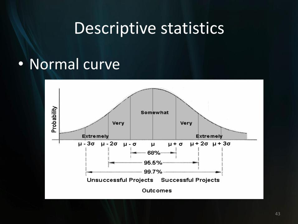
• Normal curve
43

Descriptive statistics
• Normal curve
44

Descriptive statistics
• Characteristics of normal distribution
–The normal distribution is mathematically defined.
–The normal distribution is theoretical.
–The mean, median, and mode are all the same value at the center of the distribution.
45

Descriptive statistics
• Characteristics of normal distribution
–The normal distribution is symmetrical.
–The form of a normal distribution is determined by its mean and standard deviation.
–Standard deviation can be any positive value.
46

Descriptive statistics
• Characteristics of normal distribution
–The total area under the curve is equal to 1.
–The tails of normal distribution are always approaching to x axis, but never touch it.
47

Descriptive statistics
• Normal distribution/Normal curve
–We use normal distribution to locate probabilities for scores.
–The area under the curve can be used to determine the probabilities at different points.
48

Descriptive statistics
49
Proportions of area under the normal curve

Descriptive statistics
• Normal distribution: the standard deviation indicates precisely how the scores are distributed. Empirical rule:
–About 68% of all scores lie within one standard deviation of the mean. In another word, roughly two thirds of the scores lie between one standard deviation on either side of the mean.
50

Descriptive statistics
• Normal distribution
–About 95% of all scores lie within two standard deviation of the mean (Normal scores: close to the mean).
–About 99.7% of all scores lie within three standard deviation of the mean.
51

Descriptive statistics
• In another word, we have 95% chance of selecting a score that is within 2 standard deviation of mean.
• Less than 5% scores are far from the mean (NOT normal scores).
52

Descriptive statistics
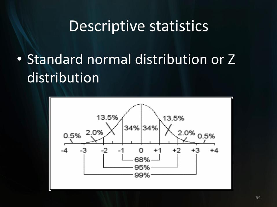
• Standard normal distribution or Z distribution
–A normal distribution with mean = 0, and standard deviation = 1.
–A Z score is a value on the x-axis of a standard normal distribution
53
Descriptive statistics
• Standard normal distribution or Z distribution
54

Descriptive statistics
• z transformation
z =𝑋−𝑀
𝑆𝐷
55
X means individual value, M is mean and SD is standard deviation. In SPSS, go to Analyze > Descriptive Statistics > Descriptives to get Z scores

Descriptive statistics
• Normal table/z table
56

Descriptive statistics
• How to use z table?
–Example: a sample of scores are approximately distributed normally with mean 8 and standard deviation 2. What is the probability of score lower than 6?
57

Descriptive statistics
• How to use z table?
–Transform a raw score 6 into a z score
–z = (6-8)/2=-1
–Check the normal table p (probability) = 0.5-0.34=0.16
–The probability of obtaining score less than 6 is 16%
58

Descriptive statistics
59

Descriptive statistics
• Descriptive statistics in SPSS
–Frequencies
–Descriptives
–Explore
60

Descriptive statistics
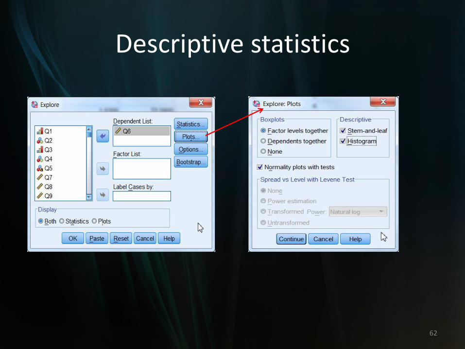
• Exercise: use 2011 YRBSS data
–Use Explore function to get descriptive statistics for Q6 (height)
–Analyze > Descriptive Statistics > Explore
61
Descriptive statistics
62

Descriptive statistics
• SPSS output
63

Descriptive statistics
• SPSS output: Normal Quantile-Quantile (Q-
Q) plot
64

Inferential statistics
• The goal of statistics is to make inferences about a population based upon information obtained in a sample.
• Hypothesis testing is the method we use to test a claim or hypothesis about a parameter in a population using observed data.
65

Inferential statistics
• Steps of hypothesis testing
–State a hypothesis
–Set the criterion
–Compare what we observe with what we expect.
–Make a decision
66

Inferential statistics
• Five elements in significance test
–Assumptions
–Hypotheses
–Test statistics
–P-value
–conclusion
67

Inferential statistics
• Assumptions
–Type of data
–Form of the population distribution
–Method of sampling
–Sample size
68

Inferential statistics
• State a hypothesis
–Null hypothesis (H0): in a hypothesis testing, we start by assuming the null hypothesis is true.
–Alternative hypothesis: directly contradicts null hypothesis
– The hypothesis testing is all about testing null hypothesis.
69

Inferential statistics
• Null hypothesis (H0): population’s values are NOT different from each other.
– Example: H0 : There is NO difference in blood pressure between treatment group and control group among patients.
– Example: H0 : μ1= μ2 or μ1- μ2 = 0
– Example: H0 : two samples are drawn from the same population.
70

Inferential statistics
• Alternative hypothesis (H1): population’s values are different from each other.
– Example: H1 = There is difference in blood pressure between treatment group and control group among patients (nondirectional-two-tailed test).
– Example: or H1 = The blood pressure of treatment group is lower than the blood pressure of control group (directional-one-tailed test).
71

Inferential statistics
• Or two samples are drawn from the different populations.
• Or H1: μ1- μ2 ≠ 0
• Or H1: μ1- μ2 > 0
• Or H1: μ1- μ2 < 0
72

Inferential statistics
• The difference in blood pressure between treatment and control group is because of random error or chance (not statistically different).
• Or the difference is large enough to conclude that blood pressure values are statistically different between two groups or because of treatment effect.
73
Inferential statistics
• Set the criterion: set the level of significance (a prespecified cutoff point)
• Typically set at 0.05 (α level) or 0.01.
• The smaller the α level, the stronger the evidence must be to reject H0.
74

Inferential statistics
• P-value
• P-value is the probability of obtaining test statistic from sample data when null hypothesis is true.
• If p-value is less than 5%, we reject the null hypothesis (why?).
75

Inferential statistics
• Compute the test statistic
• Test statistic: such as t, F values (obtained value depends on tests used in data analysis): measures the extent of apparent departure from H0.
76

Inferential statistics
• Compute the test statistic – Example: we want to know whether there is
a difference between gender in height.
– Two variables: Q2 (gender) and Q6 (height)
–We want to compare two means
–H0 : μ1 (female) = μ2 (male)
–H1: μ1 (female) ≠ μ2 (male)
77

Inferential statistics
• We use independent-samples t test to get t statistic.
78

Inferential statistics
• Compute the test statistic
– The value of test statistic is used to make a decision regarding the null hypothesis: compare test statistic to the critical value.
79

Inferential statistics
80
• Obtain critical value: it depends on degree of freedom. –A cut-off value
–We need to look at t test table for example to obtain critical value.
– If the test statistics is less than the critical value, then you fail to reject the null hypothesis.

Inferential statistics
• Make a decision
–Compare test statistic to critical value
–p value: p value is the probability of obtaining a test statistic given that null hypothesis is true.
–Significance: when p < .05, reject the null hypothesis, we reach significance.
81

Inferential statistics
• Make a decision: use t test example
–t value is -98.11
–df = 13997
–Look at t table to get critical value
• It is equal to 1.96
–t value < -1.96
–Reject Null hypothesis
82

Inferential statistics
• Critical region
83
(Neutens & Rubinson, 1997)
Inferential statistics
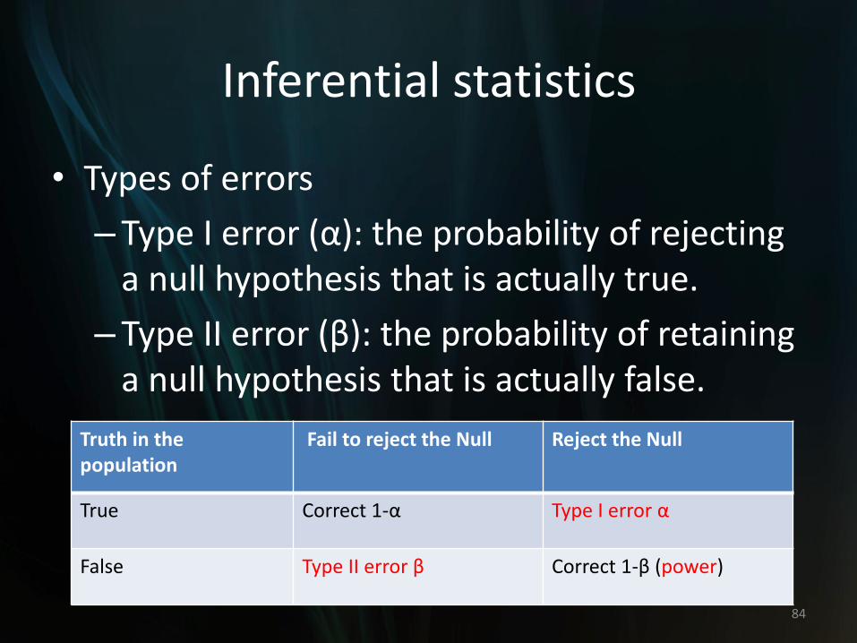
• Types of errors
– Type I error (α): the probability of rejecting a null hypothesis that is actually true.
– Type II error (β): the probability of retaining a null hypothesis that is actually false.
84
Truth in the population
Fail to reject the Null Reject the Null
True Correct 1-α Type I error α
False Type II error β Correct 1-β (power)

Inferential statistics
• Type I and Type II errors are inversely related, which means the smaller the α level, the larger the Type II error.
• To keep both errors low, large sample size is important.
85

Inferential statistics
• Power: the probability of rejecting H0
when it is in fact false.
–Power = 1-β (β is Type II error)
–Statistical power is the ability to detect a true effect.
86

Inferential statistics
• Power
• If statistical power is high, the probability of making a Type II error, or concluding there is no effect when, in fact, there is one, goes down.
87
Inferential statistics
• Power
–For example, 80% power in a clinical trial means that the study has a 80% chance of ending up with a p value of less than 5% in a statistical test (i.e. a statistically significant treatment effect) if there really was an important difference between treatments.
88

Inferential statistics
• Effect size
–Example: how much of an effect/a difference the intervention had/made (magnitude of intervention effect).
–We want to know if the intervention effect is large or small, meaningful or trivial.
89

Inferential statistics
• Effect size
–Mean difference
–Correlation coefficient
–Odds ratio
–R2
90

Inferential statistics
• The relationship between effect size and power and sample size
–When effect size increases, power increases.
–When sample size is large enough, the power increases.
–Example: Cohen’s d = M1 - M2 / spooled
91

Inferential statistics
92
• Test means: t tests and Analysis of variance
–T tests
•one sample t test
• Independent-samples t test
•Paired-samples t test

Inferential statistics
• Test means: t tests and Analysis of variance
–Analysis of variance (ANOVA)
•One-way/two-way between subject design
•One-way/two-way within subject design
•Mixed design
93
Inferential statistics
• Correlation
• Linear regression
• Non-parametric tests
– Chi-Square tests
– Sign test
– Wilcoxon signed-rank t test
– Mann-Whitney U test
– Kruskal-Wallis H test
– Friedman test
94

Inferential statistics
• SPSS demonstration
95

Inferential statistics
• SPSS demonstration
96

Inferential statistics
• SPSS demonstration
97

Inferential statistics
• SPSS demonstration
98

Inferential statistics
• T-test for two independent sample means
–Example: we want to know if there is a gender (Q2) difference in height.
–H0: µ1(Female) = µ2(Male);
–H1: µ1(Female) ≠ μ2(Male)
99

Inferential statistics
• Think about the following.
–The mean differences by two groups can be due to chance.
–sampling and measurement error.
–Tests and measuring instrument used to collect data are not perfect.
100
Inferential statistics
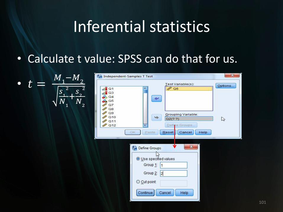
• Calculate t value: SPSS can do that for us.
• 𝑡 = 𝑀
1−𝑀
2
𝑠1
2
𝑁1
+𝑠2
2
𝑁2
101

Inferential statistics
• T-test for two independent sample means
102
t = -98.15 < tcritical = -1.96 (critical value), p < .05. There is a significant difference in height between females and males. When sample size is greater than 120, tcritical
= 1.96 at α = 0.05.

Descriptive statistics
• Confidence interval (CI) for a Mean
–“ A CI for a parameter is a range of numbers within which the parameter is believed to fall.”
103

Descriptive statistics
104

Descriptive statistics
• Standard error
–“ is the standard deviation of a sampling distribution of sample means. It is the distance that sample mean values deviate from the value of the population mean.”
105

Descriptive statistics
• How to calculate CI?
–Compute sample mean and standard error.
–Choose the level of confidence interval and find the critical value at the level of confidence.
–Compute the estimation formula to find the confidence interval
106

Descriptive statistics
• 95% CI = 𝑋 ± critical value at 95% level ( α = .05) * standard error
• Example 4: two-independent sample t-test, gender differences in height.
–We use YRBSS 2011 data.
–Q2 (Gender) and Q6 (height)
107

Descriptive statistics
• Two-Independent sample t-test: go to Analyze > Compare Means > Independent Sample T Tests
108
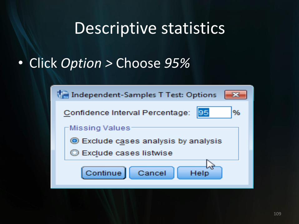
Descriptive statistics
• Click Option > Choose 95%
109

Descriptive statistics
• Output
110

Descriptive statistics
• Output
111

Descriptive statistics
• In this case, critical value = 1.96 (check t distribution table, df = ∞)
• What do we learn from the 95% CI of mean difference?
112

Basic statistics
• References
–Agresti, A. & Finlay, B. (1997). Statistical methods for the social sciences. Upper Saddle River, NJ. Prentice Hall, Inc.
–Neutens, J. J., & Rubinson, L. (1997). Research techniques for the health sciences. Needham Heights, MA. Allyn & Bacon.
113

Basic statistics
• References
–Privitera, G. J. (2012). Statistics for the behavioral sciences. Thousand Oaks, CA. SAGE Publications, Inc.
114