of quantum gates and collapsing states- a determinate ... · coulomb blockade of charge transfer....
TRANSCRIPT

International Journal of Scientific and Research Publications, Volume 2, Issue 7, July 2012 1
ISSN 2250-3153
www.ijsrp.org
OF QUANTUM GATES AND COLLAPSING
STATES- A DETERMINATE MODEL APRIORI
AND DIFFERENTIAL MODEL APOSTEORI
1DR K N PRASANNA KUMAR,
2PROF B S KIRANAGI AND
3 PROF C S BAGEWADI
ABSTRACT: We Investigate The Holistic Model With Following Composition :( 1) Mpc
(Measurement Based Quantum Computing)(2) Preparational Methodologies Of Resource States
(Application Of Electric Field Magnetic Field Etc.)For Gate Teleportation(3) Quantum Logic
Gates(4) Conditionalities Of Quantum Dynamics(5) Physical Realization Of Quantum Gates(6)
Selective Driving Of Optical Resonances Of Two Subsystems Undergoing Dipole-Dipole
Interaction By Means Of Say Ramsey Atomic Interferometry(7) New And Efficient Quantum
Algorithms For Computation(8) Quantum Entanglements And No localities(9) Computation Of
Minimum Energy Of A Given System Of Particles For Experimentation(10) Exponentially
Increasing Number Of Steps For Such Quantum Computation(11) Action Of The Quantum
Gates(12) Matrix Representation Of Quantum Gates And Vector Constitution Of Quantum
States. Stability Conditions, Analysis, Solutional Behaviour Are Discussed In Detailed For The
Consummate System. The System Of Quantum Gates And Collapsing States Show Contrast With
The Documented Information Thereto. Paper may be extended to exponential time with
exponentially increasing steps in the computation.
INTRODUCTION:
LITERATURE REVIEW:
Double quantum dots: interdot interactions, co-tunneling, and Kondo resonances without spin (See for details Qing-feng Sun, Hong Guo)
Authors show that through an interdot off-site electron correlation in a double quantum-dot (DQD)
device, Kondo resonances emerge in the local density of states without the electron spin-degree of
freedom. They also identify the physical mechanism behind this phenomenon: rather than forming a
spin singlet in the device as required in the conventional Kondo physics, that exchange of electron
position between the two quantum dots, together with the off-site Coulomb interaction, are sufficient to
induce the Kondo resonance. Due to peculiar co-tunneling events, the Kondo resonance in one dot may
be pinned at the chemical potential of the other one.
Electrical control of inter-dot electron tunneling in a quantum dot molecule( See for details K.
Müller, A. Bechtold, C. Ruppert, M. Zecherle, G. Reithmaier, M. Bichler, H.J. Krenner, G. Abstreiter, A. W. Holleitner, J. M. Villas-Bôas, J. J. Finley)
Authors employ ultrafast pump-probe spectroscopy to directly monitor electron tunneling between
discrete orbital states in a pair of spatially separated quantum dots. Immediately after excitation, several
peaks are observed in the pump-probe spectrum due to Coulomb interactions between the photo-
generated charge carriers. By tuning the relative energy of the orbital states in the two dots and
monitoring the temporal evolution of the pump-probe spectra the electron and hole tunneling times are
separately measured and resonant tunneling between the two dots is shown to be mediated both by
elastic and inelastic processes. Ultrafast (< 5 ps) int Electrons in coupled vertical quantum dots: Interdot

International Journal of Scientific and Research Publications, Volume 2, Issue 7, July 2012 2
ISSN 2250-3153
www.ijsrp.org
tunneling and Coulomb correlation
Inter dot tunneling: (See for details Garnett W. Bryant)
Interdot tunneling, lateral confinement, and Coulomb correlation determine how charge is transferred
when a bias is applied between the dots in coupled quantum dot systems. The effective-mass
Schrödinger equation for interacting electrons confined in coupled vertical double-dot systems is solved
to study interdot charge transfer. The configuration-interaction method is used to explicitly include
intradot and interdot electron correlation. The energy spectra, charge densities, and correlation functions
for interacting two-electron systems in coupled dots are presented as functions of the applied bias
between the dots. In small dots with strong lateral confinement, where the Coulomb energies are larger
than the interdot tunneling resonances, the total charge on a dot changes in integer jumps as a bias is
applied. Lateral correlation is inhibited by strong lateral confinement and charge tunneling out of a dot
is uncorrelated to the charge remaining in the dot. The dot charge changes more smoothly with applied
bias when the dots are more strongly coupled by interdot tunneling or in larger dots where intradot
correlation causes large intradot charge separation, which reduces charging energies and suppresses the
Coulomb blockade of charge transfer. In large dots, charge tunneling out of a dot remains strongly
correlated to charge left on the dot. To study charging in vertical quantum dot resonant-tunneling
structures, the dots must be wide enough that charging energies are large compared to the single-
particle-level spacings, but not so large that intradot correlation strongly suppresses the charging
energies and Coulomb blockade effects.
The Coulomb Blockade in Coupled Quantum Dots (See for details C. Livermore, C. H. Crouch, R. M. Westervelt, K. L. Campman, A. C. Gossard)
Individual quantum dots are often referred to as “artificial atoms.” Two tunnel-coupled quantum dots
can be considered an “artificial molecule.” Low-temperature measurements were made on a series
double quantum dot with adjustable interdot tunnel conductance that was fabricated in a gallium
arsenide-aluminum gallium arsenide heterostructures. The Coulomb blockade was used to determine
the ground-state charge configuration within the “molecule” as a function of the total charge on the
double dot and the interdot polarization induced by electrostatic gates. As the tunnel conductance
between the two dots is increased from near zero to 2e2/h (where e is the electron charge and h is
Planck's constant), the measured conductance peaks of the double dot exhibit pronounced changes in
agreement with many-body theory.
NANO STRUCTURES AND QUANTUM DOTS:
The properties of coupled quantum dot nanostructures depend critically on single-particle interdot
tunneling, lateral confinement, and interparticle Coulomb correlations. Calculations of few-electron and
electron-hole systems that are confined in coupled, vertical quantum dot structures have been done to
obtain a better understanding of the interplay of these effects. Authors presents the results for
symmetric and asymmetric coupled dot structures as a function of the bias applied between the dots and
the dot size. The competition between interdot tunneling and Coulomb correlation provides new optical
signatures for lateral confinement effects in quantum dots and determines which dot structures will
experience Coulomb blockade during tunneling.
Aharonov-Bohm oscillations changed by indirect interdot tunneling via electrodes in parallel-coupled
vertical double quantum dots. (See for details Hatano T, Kubo T, Tokura Y, Amaha S, Teraoka
S, Tarucha S.)
Aharonov-Bohm (AB) oscillations are studied for a parallel-coupled vertical double quantum dot with a
common source and drain electrode. Authors investigate AB oscillations of current via a one-electron
bonding state as the ground state and an antibonding state as the excited state. As the center gate voltage
becomes more negative, the oscillation period is clearly halved for both the bonding and antibonding
states, and the phase changes by half a period for the antibonding state. This result can be explained by
a calculation that takes account of the indirect interdot coupling via the two electrodes.
Quantum logic gates
A quantum logic gate is a device which performs a fixed unitary operation on selected qubits in a fixed

International Journal of Scientific and Research Publications, Volume 2, Issue 7, July 2012
ISSN 2250-3153
period of time. The gates listed below ar
describing n qubit gates are written in the computational basis
length n. The diagrams provide schematic representation of the gates.
Hadamard gate
The Hadamard gate is a common single qubit gate
The matrix is written in the computational basis
schematic representation of the gate H acting on a qubit in state
Phase gate
The phase shift gate defined as
Controlled NOT gate
The controlled-NOT (C-NOT) gate, also known as the
popular two-qubit gates. It flips the second (target) qubit if the first (control) qubit is
nothing if the control qubit is . The gate is represented by the unitary matrix
Where x,y = 0 or 1 and denotes XOR or addition modulo 2. If we apply the
in which the target qubit is and the control is either
control unchanged while the target becomes a copy of the control,
A quantum computer is any device for
mechanical phenomena to perform operations on data. In a
program's input is stored in classical
quantum computer, the input is stored in
during the computation. The reason people are excited about quantum computation is because we can
efficiently solve problems on a quantum computer which are believed to not be efficiently solvable on a
classical computer.
Experiments have already been carried out in which
on a very small number of qubits. Research in both theoretical and practical areas continues at a frantic
pace; see Quantum Information Science and Technology Roadmap
heading. Many national government and military funding agencies support quantum computing
research, to develop quantum computers for both civilian and national security purposes, such as
search Publications, Volume 2, Issue 7, July 2012
period of time. The gates listed below are common enough to have their own names. The matrices
qubit gates are written in the computational basis , where x is a binary string of
n. The diagrams provide schematic representation of the gates.
common single qubit gate H defined as
The matrix is written in the computational basis and the diagram on the right provides a
acting on a qubit in state , with x = 0,1.
and , or, in matrix notation,
NOT) gate, also known as the XOR or the measurement gate is one of the most
qubit gates. It flips the second (target) qubit if the first (control) qubit is and does
. The gate is represented by the unitary matrix
denotes XOR or addition modulo 2. If we apply the C-NOT to Boolean data
and the control is either or then the effect is to leave the
control unchanged while the target becomes a copy of the control, i.e.
is any device for computation that makes direct use of distinctively quantum
phenomena to perform operations on data. In a classical (or conventional) computer, the
bits and the computer performs operations on these bits; in a
quantum computer, the input is stored in qubits, and the quantum computer manipulates the qubits
tation. The reason people are excited about quantum computation is because we can
efficiently solve problems on a quantum computer which are believed to not be efficiently solvable on a
Experiments have already been carried out in which quantum computational operations were executed
on a very small number of qubits. Research in both theoretical and practical areas continues at a frantic
Quantum Information Science and Technology Roadmap for a sense of where the research is
ing. Many national government and military funding agencies support quantum computing
research, to develop quantum computers for both civilian and national security purposes, such as
3
www.ijsrp.org
e common enough to have their own names. The matrices
is a binary string of
and the diagram on the right provides a
, or, in matrix notation,
or the measurement gate is one of the most
and does
to Boolean data
hen the effect is to leave the
quantum
classical (or conventional) computer, the
and the computer performs operations on these bits; in a
qubits, and the quantum computer manipulates the qubits
tation. The reason people are excited about quantum computation is because we can
efficiently solve problems on a quantum computer which are believed to not be efficiently solvable on a
quantum computational operations were executed
on a very small number of qubits. Research in both theoretical and practical areas continues at a frantic
for a sense of where the research is
ing. Many national government and military funding agencies support quantum computing
research, to develop quantum computers for both civilian and national security purposes, such as

International Journal of Scientific and Research Publications, Volume 2, Issue 7, July 2012
ISSN 2250-3153
cracking public key cryptography. See for potential implementations of qu
Examples
Hadamard gate. This gate operates on a single qubit. It is represented by the Hadamard matrix:
Graphical representation of Hadamard gate
Since the rows of the matrix are orthogonal,
Phase shifter gates. Gates in this class operate on a single qubit. They are represented by 2 x 2 matrices
of the form
where θ is the phase shift.
Controlled gates. Suppose U is a gate that operates on single qubits with matrix representation
The controlled-U gate is a gate that operates on two qubits in such a way that the first qubit serves as a
control.
Graphical representation of controlled-U
Thus the matrix of the controlled U gate is as follows:
Uncontrolled gate. We note the difference between
gate
Graphical representation of uncontrolled
defined as follows:
search Publications, Volume 2, Issue 7, July 2012
public key cryptography. See for potential implementations of quantum computation.
Hadamard gate. This gate operates on a single qubit. It is represented by the Hadamard matrix:
Graphical representation of Hadamard gate
Since the rows of the matrix are orthogonal, H is indeed a unitary matrix.
gates. Gates in this class operate on a single qubit. They are represented by 2 x 2 matrices
is a gate that operates on single qubits with matrix representation
s a gate that operates on two qubits in such a way that the first qubit serves as a
U gate
gate is as follows:
Uncontrolled gate. We note the difference between the controlled-U gate and an uncontrolled
Graphical representation of uncontrolled U gate
4
www.ijsrp.org
gates. Gates in this class operate on a single qubit. They are represented by 2 x 2 matrices
s a gate that operates on two qubits in such a way that the first qubit serves as a
2 qubit

International Journal of Scientific and Research Publications, Volume 2, Issue 7, July 2012
ISSN 2250-3153
Represented by the unitary matrix
Since this gate is reducible to more elementary gates it is usually not included in the
quantum gates. It is mentioned here only to contrast it with the previous controlled gate.
Universal Quantum Gates
A set of universal quantum gates is any set of gates to which any operation possible on a quantum
computer can be reduced. One simple set of two
(H), a phase rotation gate
U such that
.
A single-gate set of universal quantum gates can also be formulated using the
gate, D(θ)
The universal classical logic gate, the
showing that all classical logic operations can be performed on a universal quantum computer.
One Qubit Gates
These have a representation as the surface of a sphere, known as the
qubit gate is to rotate one state to another. Using the Bloch Sphere picture, it is readily observed that
any such rotation can be composed of rotations about any two (non
Hence, if we can demonstrate rotation about two different axes in a
it is possible to create arbitrary one qubit rotations.
One way quantum computation (1WQC) uses an initially highly entangled state (cal
and then a pattern of single qubit measurements along different directions, together with feed
based on the results, in order to drive a quantum computation. The final result of the computation is
search Publications, Volume 2, Issue 7, July 2012
Since this gate is reducible to more elementary gates it is usually not included in the basic repertoire of
quantum gates. It is mentioned here only to contrast it with the previous controlled gate.
A set of universal quantum gates is any set of gates to which any operation possible on a quantum
d. One simple set of two-qubit universal quantum gates is the Hadamard gate
, and the controlled-NOT gate, a special case of controlled
gate set of universal quantum gates can also be formulated using the three-qubit Deutsch
The universal classical logic gate, the Toffoli gate, is reducible to the Deutsch gate,
showing that all classical logic operations can be performed on a universal quantum computer.
resentation as the surface of a sphere, known as the Bloch Sphere. The aim of a
is to rotate one state to another. Using the Bloch Sphere picture, it is readily observed that
any such rotation can be composed of rotations about any two (non-parallel) axes.
Hence, if we can demonstrate rotation about two different axes in a Physical Realization, we know that
it is possible to create arbitrary one qubit rotations.
One way quantum computation (1WQC) uses an initially highly entangled state (called a cluster state),
and then a pattern of single qubit measurements along different directions, together with feed-forward
based on the results, in order to drive a quantum computation. The final result of the computation is
5
www.ijsrp.org
basic repertoire of
A set of universal quantum gates is any set of gates to which any operation possible on a quantum
qubit universal quantum gates is the Hadamard gate
NOT gate, a special case of controlled-
qubit Deutsch
, thus
Bloch Sphere. The aim of a one
is to rotate one state to another. Using the Bloch Sphere picture, it is readily observed that
Physical Realization, we know that
led a cluster state),
forward
based on the results, in order to drive a quantum computation. The final result of the computation is
International Journal of Scientific and Research Publications, Volume 2, Issue 7, July 2012 6
ISSN 2250-3153
www.ijsrp.org
obtained by measuring the last remaining qubits in the computational basis. 1WQC was introduced by
Raussendorf and Briegl in 2001 [1]. The key feature is that the computation is not reversible since
measurement "collapses" the state of the measured qubit, effectively disentangling it from the rest of the
cluster. The essential concept underlying 1WQC is teleportation of quantum gates, extending the idea
behind linear optical QC.
The main advantage of 1WQC is that it allows scalable universal QC in systems which have a
probabilistic entangling procedure and single qubit measurements, but without a direct two-qubit
interaction suitable for implementing deterministic entangling gates.
Physical approach and perspective
Optical quantum computing (OQC) exploits measurement-based quantum computing schemes with
photons as physical qubits. The interaction between separate photonic qubits is induced by
measurement, as opposed to a direct interaction via nonlinear media. The two main physical
architectures for OQC are based on proposals by Knill, Laflamme and Milburn [1], the KLM
architecture, and by Raussendorf and Briegel, the one-way quantum computer with cluster states:
KLM allows universal and scalable OQC using only single photons, linear optics and measurement.
The by now seminal KLM work was based on the important findings of Gottesman, Chuang and
Nielsen concerning the role of teleportation for universal quantum computing. The physical resources
for universal (optical) quantum computation in the KLM scheme are multi-particle entangled states and
(entangling) multi-particle projective measurements.
Cluster state quantum computing has become an exciting alternative to existing proposals for quantum
computing, and a linear optics approach is one possible implementation. It consists of a highly
entangled multi-particle state called a cluster state, combined with single-qubit measurements and feed-
forward, which are sufficient to implement scalable, universal quantum computation. Different
algorithms only require a different “pattern” of single qubit operations on a sufficiently large cluster
state. Since only single-particle projections, together with the ability to construct the initial highly
entangled cluster state, are needed to operate such a one-way quantum computer, the cluster state
approach might offer significant technological advantages over existing schemes for quantum
computing: this includes reduced overall complexity and relaxed physical demands on the measurement
process (as compared to sensitive multi-particle projections) as well as a more efficient use of physical
resources.
Currently, the linear optics approach to quantum computation is pursued by the following European
groups: K. Banaszek (Torun, PL), F. DeMartini (Rome, IT), N. Gisin (Geneva, CH), P. Grangier
(Orsay, FR), A. Karlsson (Stockholm, SE), J. Rarity (Bristol, UK), A. Shields (Cambridge, UK), I.
Walmsley (Oxford, UK), H. Weinfurter (Munich, DE), and A. Zeilinger (Vienna, AT).
State of the art
Important key elements for linear optics quantum computation, namely the generation of entangled
states, quantum state teleportation and entanglement swapping have already been realized early in the
field (e.g. teleportation in 1997 and entanglement swapping in 1998). The latest developments include
realization of entanglement purification, freely propagating teleported qubits and feed-forward
technology.
Several practical designs implementing the KLM scheme have sequentially subsequently been
developed. Experimental methods for ultra-precise photonic quantum state creation, which serve as
ancillas in the measurement-based schemes, now achieve typical fidelities above 99%..
Enabling technologies for OQC are:
Characterization of photonic quantum states and processes. A complete, tomographic, characterization
of individual devices is indispensable for error-correction and has quite progressed within the last years.
Quantum process tomography can be used to fully characterize a quantum gate, probing it either with a
range of input states or with a single bipartite maximally entangled state, the second method being the
only viable one for continuous variable quantum processors. Based on the information gained from a
complete process characterization it was recently shown how to estimate (and bound) the error
International Journal of Scientific and Research Publications, Volume 2, Issue 7, July 2012 7
ISSN 2250-3153
www.ijsrp.org
probability per gate.
Certifying of the fidelity of processes and quantum states by means other than tomography. The larger
quantum systems becomes the more difficult it is to perform a full set of tomographic measurements.
The number of measurements necessary for a tomographic reconstruction increases exponentially with
the size of the system. In fact, even writing down the density matrix of a quantum state is a task that
grows exponentially harder with the size of the system. Novel methods to reduce the number of
.measurements necessary for a characterization of computational resources states are therefore of
imminent interest and recently several fascinating venues towards replacing tomography as the standard
tool for state characterization have become available
Development of single photons and/or entangled photon sources is required for OQC. Currently, no
source of timed single photons or entanglement is available. In the meantime, bright, albeit non-
deterministic sources of correlated photons or entangled-photon pairs are critical to allow on-going
evaluation of circuit technology as it is developed. Ultra bright and compact sources, some fiber-
coupled to improve mode quality, have been developed. Relatively brighter sources (though not yet in
absolute terms) have been demonstrated using periodically-poled nonlinear waveguides.
High-fidelity multi-qubit measurements (in the KLM scheme) and reliable preparation of multi-qubit
states (in both the KLM and the cluster state scheme).
Strengths and weaknesses
Current drawbacks of the OQC approach are low photon creation rates, low photon detection
efficiencies, and the difficulties with intermediate storage of photons in a quantum memory (see also
section 4.1.3). Advantages are obviously low decoherence (due to the photon’s weak coupling to the
environment), ultrafast processing, compatibility to fiber optics and integrated optics technologies and,
in principle, straightforward scalability of resources. A major advantage for OQC is the very short time
for one computational step achievable by using ultra-fast switches for the implementation of active
feed-forward. With present technologies this can be done in less than 100 nanoseconds [4] (in the future
probably down to 10 nanoseconds). However, the low efficiencies quoted above are presently an
important practical limitation to scalability, in the sense that they damp exponentially the success
probability of most quantum operations.
Challenges
The main challenges for OQC can be summarized as follows:
To achieve fault-tolerant quantum computing. The basic elements of fault-tolerance for OQC are
becoming well understood. It has recently been shown that also optical cluster state QC may be
performed in a fault-tolerant manner. Error models for KLM-style OQC have found that error
thresholds for gates are above 1.78%.
To reduce the resources required for OQC further and to find the limiting bounds on the required
resources. To achieve massive parallelism of qubit processing by investing in source and detector
technologies. Specifically, the development of high-flux sources of single photons and of entangled
photons as well as photon-number resolving detectors will be of great benefit to achieve this goal. To
generate high-fidelity, large multi-photon (or, more generally, many-particle) entangled states. This will
be of crucial importance for cluster state quantum computing.
To implement OQC architectures on smaller, integrated circuits. All of the current technologies involve
either free space optics or combinations of free-space optics and optical fibers. To achieve long term
scale-up, it will be essential to move to waveguide and integrated optics. Recent work has shown
tremendous progress towards that goal (see, e.g., [8]).
Computational complexity
The class of problems that can be efficiently solved by quantum computers is called BQP, for "bounded
error, quantum, and polynomial time". Quantum computers only run randomized algorithms, so BQP on
quantum computers is the counterpart of BPP on classical computers. It is defined as the set of
problems solvable with a polynomial-time algorithm, whose probability of error is bounded away from

International Journal of Scientific and Research Publications, Volume 2, Issue 7, July 2012 8
ISSN 2250-3153
www.ijsrp.org
one half. A quantum computer is said to "solve" a problem if, for every instance, its answer will be right
with high probability. If that solution runs in polynomial time, then that problem is in BQP.
BQP is suspected to be disjoint from NP-complete and a strict superset of P, but that is not known.
Both integer factorization and discrete log are in BQP. Both of these problems are NP problems
suspected to be outside BPP, and hence outside P. Both are suspected to not be NP-complete. There is a
common misconception that quantum computers can solve NP-complete problems in polynomial time.
That is not known to be true, and is generally suspected to be false.
An operator for a quantum computer can be thought of as changing a vector by multiplying it with a
particular matrix. Multiplication by a matrix is a linear operation. It has been shown that if a quantum
computer could be designed with nonlinear operators, then it could solve NP-complete problems in
polynomial time. It could even do so for #P-complete problems. It is not yet known whether such a
machine is possible.
Although quantum computers are sometimes faster than classical computers, ones of the types
described above can't solve any problems that classical computers can't solve, given enough time and
memory (albeit possibly an amount that could never practically be brought to bear). A Turing
machine can simulate these quantum computers, so such a quantum computer could never solve
an undecidable problem like the halting problem. The existence of "standard" quantum computers does
not disprove the Church-Turing thesis.
BQP
BQP, in computational complexity theory, stands for "Bounded error, Quantum, Polynomial time". It
denotes the class of problems solvable by a computer in polynomial time, with an error probability of at
most 1/4 for all instances.
In other words, there is an algorithm for a quantum computer that is guaranteed to run in polynomial
time. On any given run of the algorithm, it has a probability of at most 1/4 that it will give the wrong
answer. .
The choice of 1/4 in the definition is arbitrary. Changing the constant to any real number k such that 0
< k < 1/2 does not change the set BQP. The idea is that there is a small probability of error, but running
the algorithm many times produces an exponentially-small chance that the majority of the runs are
wrong.
The number of qubits in the computer is allowed to be a function of the instance size. For example,
algorithms are known for factoring an n-bit integer using just over 2n qubits.
Quantum computers have gained widespread interest because some problems of practical interest are
known to be in BQP, but suspected to be outside P. Currently, only three such problems are known:
Discrete logarithm
This class is defined for a quantum computer. The corresponding class for an ordinary Turing
machine plus a source of randomness is BPP.
BQP contains P and BPP and is contained in PP and PSPACE. In fact, BQP is low for PP, meaning that
a PP machine achieves no benefit from being able to solveBQP problems instantly, an indication of the
vast difference in power between these similar classes.
Microwave quantum logic gates for trapped ions (See for details C. Ospelkaus),
Control over physical systems at the quantum level is important in fields as diverse as metrology,
information processing, simulation and chemistry. For trapped atomic ions, the quantized motional and
internal degrees of freedom can be coherently manipulated with laser light. Similar control is difficult to
achieve with radio-frequency or microwave radiation: the essential coupling between internal degrees
of freedom and motion requires significant field changes over the extent of the atoms’ motion, but such
changes are negligible at these frequencies for freely propagating fields. An exception is in the near
field of microwave currents in structures smaller than the free-space wavelength where stronger
gradients can be generated. Here we first manipulate coherently (on timescales of 20 nanoseconds) the

International Journal of Scientific and Research Publications, Volume 2, Issue 7, July 2012 9
ISSN 2250-3153
www.ijsrp.org
internal quantum states of ions held in a micro fabricated trap. The controlling magnetic fields are
generated by microwave currents in electrodes that are integrated into the trap structure. We also
generate entanglement between the internal degrees of freedom of two atoms with a gate
operation suitable for general quantum computation; the entangled state has a fidelity of 0.76(3), where
the uncertainty denotes standard error of the mean. Our approach, which involves integrating the
quantum control mechanism into the trapping device in a scalable manner, could be applied to quantum
information processing, simulation and spectroscopy.
Subject terms:
Robust trapped-ion quantum logic gates by continuous dynamical decoupling P. O. Schmidt, M.
B. Plenio1, and A. Retzker
We introduce a scheme that combines phonon-mediated quantum logic gates in trapped ions with the
benefits of continuous dynamical decoupling. Authors demonstrate theoretically that a strong driving of
the qubit decouples it from external magnetic-field noise, enhancing the fidelity of two-qubit quantum
gates. Moreover, the scheme does not require ground-state cooling, and is inherently robust to undesired
ac Stark shifts. The underlying mechanism can be extended to a variety of other systems where a strong
driving protects the quantum coherence of the qubits without compromising the two-qubit couplings.
Toffoli gate
From Wikipedia, the free encyclopedia

International Journal of Scientific and Research Publications, Volume 2, Issue 7, July 2012
ISSN 2250-3153
Circuit representation of Toffoli gate
In computer science, the Toffoli gate
universal reversible logic gate, which means that any reversible circuit can be constructed from Toffoli
gates. It is also known as the "controlled
Background
A logic gate L is reversible if, for any output
a gate L is reversible, there is an inverse gate
logic gates, NOT is reversible, as can be seen from its truth table below.
INPU
T
OUTP
UT
0 1
1 0
The common AND gate is not reversible however. The inputs 00, 01 and 10 all get mapped to the
output 0.
The original motivation was that reversible
normal gate, input states are lost, since less information is present in the output than was present at the
input. This loss of information loses energy to the surrounding area(gains) as heat, bec
of thermodynamic entropy. Another way to understand this is that charges on a circuit are grounded and
thus flow away, taking a small charge of energy with them when they change state. A reversible gate
only moves the states around, and since no infor
More recent motivation comes from
transformations to be reversible but allows more general states of the computation (superpositions).
Thus, the reversible gates form a subset of gates allowed by quantum mechanics and, if we can compute
something reversibly, we can also compute it on a quantum computer.
Universality and Toffoli gate
Any reversible gate must have the same number of input and output bits, by the
For one input bit, there are two possible
gate which maps its input to the output unchanged. For two input bits, the only non
the controlled NOT gate which XORs the
Truth table Matrix form
search Publications, Volume 2, Issue 7, July 2012
Toffoli gate (also CCNOT gate), invented by Tommaso Toffoli, is a
logic gate, which means that any reversible circuit can be constructed from Toffoli
gates. It is also known as the "controlled-controlled-not" gate, which describes its action.
is reversible if, for any output y, there is a unique input x such that applying L(x) =
is reversible, there is an inverse gate L′ which maps y to x for which(x) = y. From c
logic gates, NOT is reversible, as can be seen from its truth table below.
The common AND gate is not reversible however. The inputs 00, 01 and 10 all get mapped to the
The original motivation was that reversible gates dissipate less heat (or, in principle, no heat). In a
normal gate, input states are lost, since less information is present in the output than was present at the
input. This loss of information loses energy to the surrounding area(gains) as heat, bec
thermodynamic entropy. Another way to understand this is that charges on a circuit are grounded and
thus flow away, taking a small charge of energy with them when they change state. A reversible gate
only moves the states around, and since no information is lost, energy is conserved.
More recent motivation comes from quantum computing. Quantum mechanics requires the
transformations to be reversible but allows more general states of the computation (superpositions).
subset of gates allowed by quantum mechanics and, if we can compute
something reversibly, we can also compute it on a quantum computer.
Any reversible gate must have the same number of input and output bits, by the pigeonhole principle.
For one input bit, there are two possible reversible gates. One of them is NOT. The other is the identity
gate which maps its input to the output unchanged. For two input bits, the only non-trivial gate is
which XORs the first bit to the second bit and leaves the first bit unchanged.
10
www.ijsrp.org
Tommaso Toffoli, is a
logic gate, which means that any reversible circuit can be constructed from Toffoli
L(x) = y. If
y. From common
The common AND gate is not reversible however. The inputs 00, 01 and 10 all get mapped to the
gates dissipate less heat (or, in principle, no heat). In a
normal gate, input states are lost, since less information is present in the output than was present at the
input. This loss of information loses energy to the surrounding area(gains) as heat, because
thermodynamic entropy. Another way to understand this is that charges on a circuit are grounded and
thus flow away, taking a small charge of energy with them when they change state. A reversible gate
requires the
transformations to be reversible but allows more general states of the computation (superpositions).
subset of gates allowed by quantum mechanics and, if we can compute
principle.
gates. One of them is NOT. The other is the identity
trivial gate is
first bit to the second bit and leaves the first bit unchanged.

International Journal of Scientific and Research Publications, Volume 2, Issue 7, July 2012
ISSN 2250-3153
INPU
T
OUTP
UT
0
0
0 0
0 1 0 1
1 0 1 1
1 1 1 0
Unfortunately, there are reversible functions which cannot be computed using just those gates. In other
terms, the set consisting of NOT and XOR gates is not universal (see functional completeness). If we
would like to compute an arbitrary function by reve
the Toffoli gate, proposed in 1980 by Toffoli.
This gate has a 3-bit input and output. If the first two bits are set, it flips the third bit. Following is a
table over the input and output bits(For
Truth table Matrix form
INPUT OUTPU
T
0
0
0
0
0
0
0 0 1 0 0 1
0 1 0 0 1 0
0 1 1 0 1 1
1 0 0 1 0 0
1 0 1 1 0 1
1 1 0 1 1 1
1 1 1 1 1 0
It can be also described as mapping bits a,
The Toffoli gate is universal; this means that for any
consisting of Toffoli gates which takes
outputs x1, x2, ..., xm, f(x1, x2, ..., xm), and some extra bits (called garbage). Essentially, this means
that one can use Toffoli gates to build systems that will perform any desired boolean function
computation in a reversible manner.
Related logic gates (Figures are taken from the Home Page of Wikipedia)
search Publications, Volume 2, Issue 7, July 2012
Unfortunately, there are reversible functions which cannot be computed using just those gates. In other
terms, the set consisting of NOT and XOR gates is not universal (see functional completeness). If we
would like to compute an arbitrary function by reversible gates, we need another gate. One possibility is
Toffoli gate, proposed in 1980 by Toffoli.
bit input and output. If the first two bits are set, it flips the third bit. Following is a
For more details see Stanford Encyclopedia and Wikipedia)
It can be also described as mapping bits a, b and c to a, b and c XOR (a AND b).
The Toffoli gate is universal; this means that for any boolean function f(x1, x2, ..., xm), there is a circuit
consisting of Toffoli gates which takes x1, x2, ..., xm and some extra bits set to 0 or 1 and
xm), and some extra bits (called garbage). Essentially, this means
that one can use Toffoli gates to build systems that will perform any desired boolean function
e taken from the Home Page of Wikipedia)
11
www.ijsrp.org
Unfortunately, there are reversible functions which cannot be computed using just those gates. In other
terms, the set consisting of NOT and XOR gates is not universal (see functional completeness). If we
rsible gates, we need another gate. One possibility is
bit input and output. If the first two bits are set, it flips the third bit. Following is a
xm), there is a circuit
and some extra bits set to 0 or 1 and
xm), and some extra bits (called garbage). Essentially, this means
that one can use Toffoli gates to build systems that will perform any desired boolean function

International Journal of Scientific and Research Publications, Volume 2, Issue 7, July 2012 12
ISSN 2250-3153
www.ijsrp.org
.
Relation to quantum computing
Any reversible gate can be implemented on a quantum computer, and hence the Toffoli gate is also a
quantum operator. However, the Toffoli gate cannot be used for universal quantum computation,
though it does mean that a quantum computer can implement all possible classical computations. The
Toffoli gate has been successfully realized in January 2009 at the University of Innsbruck, Austria.
In his celebrated paper Adolf Haimovici (3), studied the growth of a two species ecological system
divided on age groups. In this paper, we establish that his processual regularities and procedural
formalities can be applied for consummation of a system of oxygen consumption by terrestrial
organisms. Notations are changed towards the end of obtaining higher number of equations in the
holistic study of the global climate models. Quintessentially, Haimovician diurnal dynamics are used to
draw interesting inferences, from the simple fact that terrestrial organisms consume oxygen due to
cellular respiration.
Entanglement a resource for Quantum Computation:
Pursuant to their interaction,, quantum particles generally behave inexorable and inextricably as a
single nonseparable entangled consummate and consolidated system The concept of entanglement
plays an essential role in quantum physics. Many a physicist have resorted to experimentation in so far
as entanglement is concerned, some of them with Rydberg atoms and microwave photons in a cavity
and tested quantum mechanics in situations of increasing complexity. Entanglement, it is reported that
resulted either from a resonant exchange of energy between atoms and the cavity field or from
dispersive energy shifts affecting atoms and photons when they were not resonant. With two entangled
particles (two atoms or one atom and a photon), . This has lead to consummation of the newer
configuration of new versions of the Einstein-Podolsky-Rosen situation. The detection of one particle
projected the other, at a distance, in a correlated state. This process could be viewed as an elementary
measurement, one particle being a ‘‘meter’’ measuring the other. Raimond etal. performed a ‘‘quantum
nondemolition’’ measurement of a single photon, which was detected repeatedly without destroying it.
Entanglement is also essential to understand decoherence, the process accounting for the classical
appearance of the macroscopic world. A mesoscopic superposition of states (‘‘Schrõdinger cat’’) gets
rapidly entangled with its environment, losing its quantum coherence. We have prepared a Schrõdinger
cat made of a few photons and studied the dynamics of its decoherence, in an experiment which
constitutes a glimpse at the quantum/classical boundary. Entanglement is also used as a resource for
the processing of quantum information. By using quantum two-state systems (qubits) instead of
classical bits of information, one can perform logical operations exploiting quantum interferences and
taking advantage of the properties of entanglement. Manipulating as qubits atoms and photons in a
cavity, we have operated a quantum gate and applied it to the generation of a complex three-particle
entangled state

International Journal of Scientific and Research Publications, Volume 2, Issue 7, July 2012 13
ISSN 2250-3153
www.ijsrp.org
PREPARATION OF RESOURCE STATES SUITABLE FOR GATE TELEPORATATION
AND MBQC(MEASUREMENT BASED QUANTUM COMPUTATION): MODULE NUMBERED ONE:
NOTATION :
��� : CATEGORY ONE OF MBQC
��� : CATEGORY TWO OF MBQC
��� : CATEGORY THREE OF MBQC
��� :CATEGORY ONE OF RESOURCE STATES SUITABLE FOR TELEPORATATION
��� : CATEGORY TWO OF RESOURCE STATES SUITABLE FOR TELEPORATATION
��� : CATEGORY THREE OF RESOURCE STATES SUITABLE FOR TELEPORATATION
CONDITIONALITIES OF QUANTUM DYNAMICS(EXERCISE OF MAGNETIC FIELD,
ELECTRIC FIELD ETC., EXPERIMENTAL CONDITIONS) AND QUANTUM LOGIC GATE:
MODEULE NUMBERED TWO
=========================================================================
��� : CATEGORY ONE OF QUANTUM LOGIC GATES
�� : CATEGORY TWO OF QUANTUM LOGIC GATES
�� :CATEGORY THREE OF QUANTUM LOGIC STATES
��� : CATEGORY ONE OF CONDITIONALITIES OF QUANTUM DYNAMICS
�� : CATEGORY TWO OF CONDITIONALITIES OF QUANTUM DYNAMICS
�� : CATEGORY THREE OF CONDITIONALITIES OF QUANTUM DYNAMICS
QUANTUM GATES(PHYSICAL REALISATION OF QUANTUM GATES) AND RAMSEY
ATOMIC INTERFEROMETRY METHODOLOGY USING AND INDUCED SELECTIVE
DRIVING OF OPTICAL RESONANCES OF TWQO SUBSYSTEMS UNDERGOING DIPOLE
DIPOLE INTERACTION : MODULE NUMBERED THREE
=========================================================================
��� : CATEGORY ONE OF INDUCED”SELECTIVE DRIVING OF OPTICAL RESONANCES OF
TWO SUBSYSTEMS UNDERGOING DIPOLE-DIPOLE INTERACTION
��� : CATEGORY TWO OF INDUCED “SELECTIVE DRIVING OF OPTICAL RESONANCES OF
TWO SUBSYSTEMS UNDRGOING DIPOLE-DIPOLE INTERACTION”
��� : CATEGORY THREE OF INDUCED “SELECTIVE DRIVING OF OPTICAL RESONANCES
OF TWO SUBSYSTEMS UNDERGOING DIPOLE-DIPOLE INTERACTION”
��� : CATEGORY ONE OF THE PHYSICAL REALISATION OF QUANTUM GATES
��� : CATEGORY TWO OF PHYSICAL REALISATIONS OF QUANTUM GATES
��� : CATEGORY THREE OF QUANTUM GATES(PHYSICAL REALISATION THEREOF)
QUANTUM ENTAGLEMENT AND NONLOCALITY AND NEW EFFCIENT ALGORITHMS:

International Journal of Scientific and Research Publications, Volume 2, Issue 7, July 2012 14
ISSN 2250-3153
www.ijsrp.org
MODULE NUMBERED FOUR:
=========================================================================
��� : CATEGORY ONE OF QUANTUM ENTANGLEMENTS AND OR NONLOCALITIES
��� : CATEGORY TWO OF QUANTUM ENTANGLEMENTS AND NONLOCALITIES
��� :CATEGORY THREE OF QUANTUM ENTANGLEMENTS AND NONLOCALITIES
��� :CATEGORY ONE OF SET OF EFFCIENT ALGORITHMS
��� : CATEGORY TWO OF SET OF EFFCIENT ALGORITHMS ��� : CATEGORY THREE OF SET OF NEW AND EFFCIENT ALGORITHMS SET
COMPUTATIONAL COMPLEXITY OR THE EXPONENTIALLY INCREASING NUMBER
OF STEPS IN A SYSTEM OF PARTICLES AND COMPUTATION OF THE MINIMUM
ENERGY OF SYSTEM OF PARTICLES: MODULE NUMBERED FIVE:
=========================================================================
=========
�� : CATEGORY ONE OF EXPONENTIALLY INCREASING NUMBER OF STEPS INA SYSTEM
OF PARICLES DURING QUANTUM COMPUTATION
�� : CATEGORY TWO OF EXPONENTIALLY INCREASING NUMBER OF STEPS INA
SYSTEM OF PARTICLES BELONGING TO ANOTHER CATEGORY THAN THAT OF
CATEGORY ONE DURING QUANTUM COMPUTATION
��� : CATEGORY THREE OF EXPONENTIALLY INCREASING NUMBER IOF STEPS IN A
SYSTEM OF PARTCILES DURING QUANTUM COMPUTATION BELONGING TO DIFFERENT
CATEGORY(HERE CATEGORY THREE)
�� : CATEGORY ONE OF QUANTUM COMPUTATION OF THE MINIMUM ENERGY OF A
GIVEN SYSTEM OF NUMBERABLE PARTICLES
�� : CATEGORY TWO OF QUANTUM COMPUTATION OF MINUM ENERGY OF SOME
SYSTEM OF PARTCILES OTHER THAN CATEGORY ONE ��� : CATEGORY THREE OF QUANTUM COMPUTATION OF THE MINIMUM ENERGY OF
SOME SYSTEM OF PARTCILES UNDER STUDY BELONGING TO CATEGORY OTHER THAN
THE ONE MENTIONED IN THE FOREGOING
ACTION OF QUANTUM GATES AND MATRIX REPRESENTATION OF THE GATE AND
VECTOR CONSTITUTION OF QUANTUM STATE: MODULE NUMBERED SIX(NOTE
THAT THERE IS ALWAYS A TIME LAG IN SUCH A DISSSIPATION PROCESS)
==========================================================================

International Journal of Scientific and Research Publications, Volume 2, Issue 7, July 2012 15
ISSN 2250-3153
www.ijsrp.org
��� : CATEGORY ONE OF MATRIX REPRESENTATION OF THE QUANTUM GATE AND
VECTOR CONSTITUTION OF QUANTUM STATE AND CONCOMITANT ACTION OF THE
QUABNTUM GATE
��� :CATEGORY TWO OF THE MATRIX REPRESENTATION OF THE QUANTUM GATE AND
VECTOR CONSTITUTION OF QUANTUM STATETO THE CONCOMITANT AND
CORRESPONDING OF THE ACTION OF QUANTUM GATE CLASSIFIED BELOW
��� : CATEGORY THREE OF THE MATRIOX RESENTATION OF QUANTUM GATE AND
VECTOR CONSTITUTION OF THE QUANTUM STATE TO THE CONCOMITANT ACTION OF
THE QUANTUM GATE CLASSIFIED BELOW
��� : CATEGORY ONE OF THE ACTION OF THE CORESPONDING QUANTUM GATES
��� : CATEGORY TWO OF THE ACTION OF THE CORRESPONDING QUANTUM GATES ��� :CATEGORY THREE OF THE ACTION OF THE CORRESPONDING QUANTUM GATES
ACCENTUATION COEFFCIENTS OF
THE HOLISTIC SYSTEM:
(1)MBQC(MEASUREMENT BASED QUANTUM COMPUTING)
(2) PREPARATIONAL METHODOLOGIES OF RESOURCE STATES (APPLICATION OF
ELECTRIC FIELD MAGNETCI FIELD ETC.)FOR GATE TELEPORATATION
(3) QUANTUM LOGIC GATES
(4) CONDITIONALITIES OF QUANTUM DYNAMICS
(5) PHYSICAL REALISATION OF QUANTUM GATES
(6) SELECTIVE DRIVING OF OPTICAL RESONANCES OF TWO SUBSYSTEMS
UNDERGOING DIPOLE-DIPOLE INTERACTION BY MEANS OF SAY RAM,SEY ATOMIC
INTERFEROMETRY
(7) NEW AND EFFCIENT QUANTUM ALGORITHMS FOR COMPUTATION
(8) QUANTUM ENTANGLEMENTS AND NONLOCALITIES
(9) COMPUTATION OF MINIMUM ENERGY OF A GIVEN SYSTEM OF PARTICLES FOR
EXPERIMENTATION
(10) EXPONENTIALLY INCRESING NUMBER OF STEPS FOR SUCH QUANTUM
COMPUTATION
(11) ACTION OF THE QUANTUM GATES
(12) MATRIX REPRESENTATION OF QUANTUM GATES AND VECTOR CONSTITUTION
OF QUANTUM STATES
==========================================================================
��������, ��������, ��������, ��������, ��������, �������� ��������, �������, ������� ��������, �������, �������: ��������, ��������, �������� , ��������, ��������, ��������

International Journal of Scientific and Research Publications, Volume 2, Issue 7, July 2012 16
ISSN 2250-3153
www.ijsrp.org
��������, ��������, ��������, ��������, ��������, ��������, �������, ��� ����, ��������,�������, ��� ����, ��������, ��������, ��������, ��������, ��������, ��������, �������� DISSIPATION COEFFICIENTS OF THE HOLISTIC SYSTEM:
========================================================================
����′ ����, ����′ ����, ����′ ����, ����′ ����, ����′ ����, ����′ ����, ����′ ����, ���′ ����, ���′ ����, ����′ ����, ���′ ����, ���′ ���� , ����′ ����, ����′ ����, ����′ ����, ����′ ����, ����′ ����, ����′ ���� ����′ ����, ����′ ����, ����′ ����, ����′ ����, ����′ ����, ����′ ����, ���′ ����, ��� ′ ����, ����′ ���� ���′ ����, ��� ′ ����, ����′ ���� , ����′ ����, ����′ ����, ����′ ����, ����′ ����, ����′ ����, ����′ ����
GOVERNING EQUATIONS: SYSTEM: 1) MBQC (MEASUREMENT BASED QUANTUM
COMPUTING) (2) PREPARATIONAL METHODOLOGIES OF RESOURCE STATES
(APPLICATION OF ELECTRIC FIELD MAGNETCI FIELD ETC.)FOR GATE
TELEPORATATION
The differential system of this model is now
������ = ����������� − �����′ ���� + ����′′ ��������, ������
��� �� = ����������� − �����′ ���� + ����′′ ��������, ������
���!�� = ����������� − "����′ ���� + ����′′ ��������, ��# ���
�$���� = ����������� − �����′ ���� − ����′′ ������, ������
�$� �� = ����������� − �����′ ���� − ����′′ ������, ������
�$�!�� = ����������� − "����′ ���� − ����′′ ������, ��# ���
+����′′ ��������, �� = First augmentation factor −����′′ ������, �� = First detritions factor
GOVERNING EQUATIONS:SYSTEM NUMBERED TWO: 3) QUANTUM LOGIC GATES(4)
CONDITIONALITIES OF QUANTUM DYNAMICS
The differential system of this model is now
���%�� = ���������� − �����′ ���� + ����′′ �������, ������
���&�� = ���������� − ����′ ���� + ���′′ �������, �����
���'�� = ��������� − ����′ ���� + ���′′ �������, �����

International Journal of Scientific and Research Publications, Volume 2, Issue 7, July 2012 17
ISSN 2250-3153
www.ijsrp.org
�$�%�� = ���������� − �����′ ���� − ����′′ �������� �, ������
�$�&�� = ���������� − ����′ ���� − ���′′ �������� �, �����
�$�'�� = ��������� − ����′ ���� − ���′′ �������� �, �����
+����′′ �������, �� = First augmentation factor
−����′′ �������� �, �� = First detritions factor
GOVERNING EQUATIONS: 5) PHYSICAL REALISATION OF QUANTUM GATES(6)
SELECTIVE DRIVING OF OPTICAL RESONANCES OF TWO SUBSYSTEMS
UNDERGOING DIPOLE-DIPOLE INTERACTION BY MEANS OF SAY RAM,SEY ATOMIC
INTERFEROMETRY
The differential system of this model is now
��()�� = ����������� − �����′ ���� + ����′′ ��������, ������
��(��� = ����������� − �����′ ���� + ����′′ ��������, ������
��((�� = ����������� − �����′ ���� + ����′′ ��������, ������
�$()�� = ����������� − �����′ ���� − ����′′ ��������, ������
�$(��� = ����������� − �����′ ���� − ����′′ ��������, ������
�$((�� = ����������� − �����′ ���� − ����′′ ��������, ������ +����′′ ��������, �� = First augmentation factor
−����′′ ��������, �� = First detritions factor
GOVERNING EQUATIONS: 7) NEW AND EFFCIENT QUANTUM ALGORITHMS FOR
COMPUTATION(8) QUANTUM ENTANGLEMENTS AND NONLOCALITIES
The differential system of this model is now
��( �� = ����������� − �����′ ���� + ����′′ ��������, ������
��(!�� = ����������� − "����′ ���� + ����′′ ��������, ��# ���
��(%�� = ����������� − �����′ ���� + ����′′ ��������, ������

International Journal of Scientific and Research Publications, Volume 2, Issue 7, July 2012 18
ISSN 2250-3153
www.ijsrp.org
�$( �� = ����������� − �����′ ���� − ����′′ ���������, ������
�$(!�� = ����������� − "����′ ���� − ����′′ ���������, ��# ���
�$(%�� = ����������� − �����′ ���� − ����′′ ���������, ������
+����′′ ��������, �� = First augmentation factor
−����′′ ���������, �� = First detritions factor
GOVERNING EQUATIONS: (9) COMPUTATION OF MINIMUM ENERGY OF A GIVEN
SYSTEM OF PARTICLES FOR EXPERIMENTATION(10) EXPONENTIALLY INCRESING
NUMBER OF STEPS FOR SUCH QUANTUM COMPUTATIONMODULE NUMBERED FIVE
The differential system of this model is now
��('�� = ��������� − ����′ ���� + ���′′ ������� , �����
��(*�� = ��� ������ − ���� ′ ���� + ��� ′′ ������� , �����
���)�� = ���������� − �����′ ���� + ����′′ ������� , ������
�$('�� = ��������� − ����′ ���� − ���′′ ����������, �����
�$(*�� = ��� ������ − ���� ′ ���� − ��� ′′ ����������, �����
�$�)�� = ���������� − �����′ ���� − ����′′ ����������, ������
+���′′ ������� , �� = First augmentation factor
−���′′ ����������, �� = First detritions factor
GOVERNING EQUATIONS: 11) ACTION OF THE QUANTUM GATES(12) MATRIX
REPRESENTATION OF QUANTUM GATES AND VECTOR CONSTITUTION OF
QUANTUM STATES(LOGARITHMIC APPLICATION DERIVATION)
The differential system of this model is now
���(�� = ����������� − �����′ ���� + ����′′ ��������, ������
������ = ����������� − �����′ ���� + ����′′ ��������, ������
��� �� = ����������� − �����′ ���� + ����′′ ��������, ������

International Journal of Scientific and Research Publications, Volume 2, Issue 7, July 2012 19
ISSN 2250-3153
www.ijsrp.org
�$�(�� = ����������� − �����′ ���� − ����′′ ����������, ������
�$���� = ����������� − �����′ ���� − ����′′ ����������, ������
�$� �� = ����������� − �����′ ���� − ����′′ ����������, ������
+����′′ ��������, �� = First augmentation factor
−����′′ ����������, �� = First detritions factor
GOVERNING EQUATIONS OF THE HOLISTIC SYSTEM:
THE HOLISTIC SYSTEM:
(1)MBQC(MEASUREMENT BASED QUANTUM COMPUTING)
(2) PREPARATIONAL METHODOLOGIES OF RESOURCE STATES (APPLICATION OF
ELECTRIC FIELD MAGNETCI FIELD ETC.)FOR GATE TELEPORATATION
(3) QUANTUM LOGIC GATES
(4) CONDITIONALITIES OF QUANTUM DYNAMICS
(5) PHYSICAL REALISATION OF QUANTUM GATES
(6) SELECTIVE DRIVING OF OPTICAL RESONANCES OF TWO SUBSYSTEMS
UNDERGOING DIPOLE-DIPOLE INTERACTION BY MEANS OF SAY RAM,SEY ATOMIC
INTERFEROMETRY
(7) NEW AND EFFCIENT QUANTUM ALGORITHMS FOR COMPUTATION
(8) QUANTUM ENTANGLEMENTS AND NONLOCALITIES
(9) COMPUTATION OF MINIMUM ENERGY OF A GIVEN SYSTEM OF PARTICLES FOR
EXPERIMENTATION
(10) EXPONENTIALLY INCRESING NUMBER OF STEPS FOR SUCH QUANTUM
COMPUTATION
(11) ACTION OF THE QUANTUM GATES
(12) MATRIX REPRESENTATION OF QUANTUM GATES AND VECTOR CONSTITUTION
OF QUANTUM STATES
=========================================================================
������ = ����������� − + ����′ ���� +����′′ ��������, �� +����′′ ���,�,����, �� +����′′ ���,�,�����, �� +����′′ ���,�,�,�,�����, �� +���′′ ���,�,�,�,���� , �� +����′′ ���,�,�,�,�����, �� , ���
��� �� = ����������� − + ����′ ���� +����′′ ��������, �� +���′′ ���,�,����, �� +����′′ ���,�,�����, �� +����′′ ���,�,�,�,�����, �� +��� ′′ ���,�,�,�,���� , �� +����′′ ���,�,�,�,�����, �� , ���

International Journal of Scientific and Research Publications, Volume 2, Issue 7, July 2012 20
ISSN 2250-3153
www.ijsrp.org
���!�� = ����������� − + ����′ ���� +����′′ ��������, �� +���′′ ���,�,����, �� +����′′ ���,�,�����, �� +����′′ ���,�,�,�,�����, �� +����′′ ���,�,�,�,���� , �� +����′′ ���,�,�,�,�����, �� , ���
Where ����′′ ��������, �� , ����′′ ��������, �� , ����′′ ��������, �� are first augmentation coefficients for
category 1, 2 and 3
+����′′ ���,�,����, �� , +���′′ ���,�,����, �� , +���′′ ���,�,����, �� are second augmentation coefficient
for category 1, 2 and 3
+����′′ ���,�,�����, �� , +����′′ ���,�,�����, �� , +����′′ ���,�,�����, �� are third augmentation coefficient for
category 1, 2 and 3
+����′′ ���,�,�,�,�����, �� , +����′′ ���,�,�,�,�����, �� , +����′′ ���,�,�,�,�����, �� are fourth augmentation
coefficient for category 1, 2 and 3
+���′′ ���,�,�,�,���� , �� , +��� ′′ ���,�,�,�,���� , �� , +����′′ ���,�,�,�,���� , �� are fifth augmentation
coefficient for category 1, 2 and 3
+����′′ ���,�,�,�,�����, �� , +����′′ ���,�,�,�,�����, �� , +����′′ ���,�,�,�,�����, �� are sixth augmentation
coefficient for category 1, 2 and 3
�$���� = ����������� − - ����′ ���� −����′′ ������, �� −����′′ ���,�,���� , �� – ����′′ ���,�,�����, �� −����′′ ���,�,�,�,����, �� −���′′ ���,�,�,�,�����, �� −����′′ ���,�,�,�,�����, �� / ���
�$� �� = ����������� − + ����′ ���� −����′′ ������, �� −���′′ ���,�,���� , �� – ����′′ ���,�,�����, �� −����′′ ���,�,�,�,����, �� −��� ′′ ���,�,�,�,�����, �� −����′′ ���,�,�,�,�����, �� , ���
�$�!�� = ����������� − + ����′ ���� −����′′ ������, �� −���′′ ���,�,���� , �� – ����′′ ���,�,�����, �� −����′′ ���,�,�,�,����, �� −����′′ ���,�,�,�,�����, �� −����′′ ���,�,�,�,�����, �� , ���
Where −����00 ������, �� , −����00 ������, �� , −����00 ������, �� are first detrition coefficients for category
1, 2 and 3
−����00 ���,�,���� , �� , −���00 ���,�,���� , �� , −���00 ���,�,���� , �� are second detrition coefficients for
category 1, 2 and 3
−����00 ���,�,�����, �� , −����00 ���,�,�����, �� , −����00 ���,�,�����, �� are third detrition coefficients for
category 1, 2 and 3
−����00 ���,�,�,�,����, �� , −����00 ���,�,�,�,����, �� , −����00 ���,�,�,�,����, �� are fourth detrition
coefficients for category 1, 2 and 3
−���00 ���,�,�,�,�����, �� , −��� 00 ���,�,�,�,�����, �� , −����00 ���,�,�,�,�����, �� are fifth detrition coefficients
for category 1, 2 and 3
−����00 ���,�,�,�,�����, �� , −����00 ���,�,�,�,�����, �� , −����00 ���,�,�,�,�����, �� are sixth detrition

International Journal of Scientific and Research Publications, Volume 2, Issue 7, July 2012 21
ISSN 2250-3153
www.ijsrp.org
coefficients for category 1, 2 and 3
���%�� = ���������� − + ����0 ���� +����00 �������, �� +����00 ���,�,�����, �� +����00 ���,�,������, �� +����00 ���,�,�,�,������, �� +���00 ���,�,�,�,����� , �� +����00 ���,�,�,�,������, �� , ���
���&�� = ���������� − + ���0 ���� +���00 �������, �� +����00 ���,�,�����, �� +����00 ���,�,������, �� +����00 ���,�,�,�,������, �� +��� 00 ���,�,�,�,����� , �� +����00 ���,�,�,�,������, �� , ��
���'�� = ��������� − + ���0 ���� +���00 �������, �� +����00 ���,�,�����, �� +����00 ���,�,������, �� +����00 ���,�,�,�,������, �� +����00 ���,�,�,�,����� , �� +����00 ���,�,�,�,������, �� , ��
Where +����00 �������, �� , +���00 �������, �� , +���00 �������, �� are first augmentation coefficients for
category 1, 2 and 3
+����00 ���,�,�����, �� , +����00 ���,�,�����, �� , +����00 ���,�,�����, �� are second augmentation coefficient
for category 1, 2 and 3
+����00 ���,�,������, �� , +����00 ���,�,������, �� , +����00 ���,�,������, �� are third augmentation coefficient
for category 1, 2 and 3
+����00 ���,�,�,�,������, �� , +����00 ���,�,�,�,������, �� , +����00 ���,�,�,�,������, �� are fourth augmentation
coefficient for category 1, 2 and 3
+���00 ���,�,�,�,����� , �� , +��� 00 ���,�,�,�,����� , �� , +����00 ���,�,�,�,����� , �� are fifth augmentation
coefficient for category 1, 2 and 3
+����00 ���,�,�,�,������, �� , +����00 ���,�,�,�,������, �� , +����00 ���,�,�,�,������, �� are sixth augmentation
coefficient for category 1, 2 and 3
�$�%�� = ���������� − + ����0 ���� −����00 ������� , �� −����00 ���,�,���, �� – ����00 ���,�,�,�����, �� −����00 ���,�,�,�,�����, �� −���00 ���,�,�,�,������, �� −����00 ���,�,�,�,������, �� , ���
�$�&�� = ���������� − + ���0 ���� −���00 ������� , �� −����00 ���,�,���, �� – ����00 ���,�,�,�����, �� −����00 ���,�,�,�,�����, �� −��� 00 ���,�,�,�,������, �� −����00 ���,�,�,�,������, �� , ��
�$�'�� = ��������� − + ���0 ���� −���00 ������� , �� −����00 ���,�,���, �� – ����00 ���,�,�,�����, �� −����00 ���,�,�,�,�����, �� −����00 ���,�,�,�,������, �� −����00 ���,�,�,�,������, �� , ��
where −�b��00 �����G� , t� , −�b�00 �����G� , t� , −�b�00 �����G� , t� are first detrition coefficients for
category 1, 2 and 3
−����00 ���,�,���, �� , −����00 ���,�,���, �� , −����00 ���,�,���, �� are second detrition coefficients for
category 1,2 and 3
−����00 ���,�,�,�����, �� , −����00 ���,�,�,�����, �� , −����00 ���,�,�,�����, �� are third detrition coefficients for

International Journal of Scientific and Research Publications, Volume 2, Issue 7, July 2012 22
ISSN 2250-3153
www.ijsrp.org
category 1,2 and 3
−����00 ���,�,�,�,�����, �� , −����00 ���,�,�,�,�����, �� , −����00 ���,�,�,�,�����, �� are fourth detrition
coefficients for category 1,2 and 3
−���00 ���,�,�,�,������, �� , −��� 00 ���,�,�,�,������, �� , −����00 ���,�,�,�,������, �� are fifth detrition
coefficients for category 1,2 and 3
−����00 ���,�,�,�,������, �� , −����00 ���,�,�,�,������, �� , −����00 ���,�,�,�,������, �� are sixth detrition
coefficients for category 1,2 and 3
��()�� =����������� − - ����0 ���� +����00 ��������, �� +����00 ���,�,�����, �� +����00 ���,�,�,�����, �� +����00 ���,�,�,�,�,������, �� +���00 ���,�,�,�,�,����� , �� +����00 ���,�,�,�,�,������, �� / ���
��(��� =����������� − + ����0 ���� +����00 ��������, �� +���00 ���,�,�����, �� +����00 ���,�,�,�����, �� +����00 ���,�,�,�,�,������, �� +��� 00 ���,�,�,�,�,����� , �� +����00 ���,�,�,�,�,������, �� , ���
��((�� =����������� − + ����0 ���� +����00 ��������, �� +���00 ���,�,�����, �� +����00 ���,�,�,�����, �� +����00 ���,�,�,�,�,������, �� +����00 ���,�,�,�,�,����� , �� +����00 ���,�,�,�,�,������, �� , ���
+����00 ��������, �� , +����00 ��������, �� , +����00 ��������, �� are first augmentation coefficients for
category 1, 2 and 3
+����00 ���,�,�����, �� , +���00 ���,�,�����, �� , +���00 ���,�,�����, �� are second augmentation
coefficients for category 1, 2 and 3
+����00 ���,�,�,�����, �� , +����00 ���,�,�,�����, �� , +����00 ���,�,�,�����, �� are third augmentation coefficients
for category 1, 2 and 3
+����00 ���,�,�,�,�,������, �� , +����00 ���,�,�,�,�,������, �� , +����00 ���,�,�,�,�,������, �� are fourth
augmentation coefficients for category 1, 2 and 3
+���00 ���,�,�,�,�,����� , �� , +��� 00 ���,�,�,�,�,����� , �� , +����00 ���,�,�,�,�,����� , �� are fifth augmentation
coefficients for category 1, 2 and 3
+����00 ���,�,�,�,�,������, �� , +����00 ���,�,�,�,�,������, �� , +����00 ���,�,�,�,�,������, �� are sixth augmentation
coefficients for category 1, 2 and 3
�$()�� =

International Journal of Scientific and Research Publications, Volume 2, Issue 7, July 2012 23
ISSN 2250-3153
www.ijsrp.org
����������� − + ����0 ���� −����00 ��������, �� – ����00 ���,�,����� , �� – ����00 ���,�,�,���, �� −����00 ���,�,�,�,�,�����, �� −���00 ���,�,�,�,�,������, �� −����00 ���,�,�,�,�,������, �� , ���
�$(��� =����������� − + ����0 ���� −����00 ��������, �� – ���00 ���,�,����� , �� – ����00 ���,�,�,���, �� −����00 ���,�,�,�,�,�����, �� −��� 00 ���,�,�,�,�,������, �� −����00 ���,�,�,�,�,������, �� , ���
�$((�� =����������� − + ����0 ���� −����00 ��������, �� – ���00 ���,�,����� , �� – ����00 ���,�,�,���, �� −����00 ���,�,�,�,�,�����, �� −����00 ���,�,�,�,�,������, �� −����00 ���,�,�,�,�,������, �� , ���
−����00 ��������, �� , −����00 ��������, �� , −����00 ��������, �� are first detrition coefficients for
category 1, 2 and 3
−����00 ���,�,����� , �� , −���00 ���,�,����� , �� , −���00 ���,�,����� , �� are second detrition coefficients
for category 1, 2 and 3
−����00 ���,�,�,���, �� , −����00 ���,�,�,���, �� , −����00 ���,�,�,���, �� are third detrition coefficients for
category 1,2 and 3
−����00 ���,�,�,�,�,�����, �� , −����00 ���,�,�,�,�,�����, �� , −����00 ���,�,�,�,�,�����, �� are fourth detrition
coefficients for category 1, 2 and 3
−���00 ���,�,�,�,�,������, �� , −��� 00 ���,�,�,�,�,������, �� , −����00 ���,�,�,�,�,������, �� are fifth detrition
coefficients for category 1, 2 and 3
−����00 ���,�,�,�,�,������, �� , −����00 ���,�,�,�,�,������, �� , −����00 ���,�,�,�,�,������, �� are sixth detrition
coefficients for category 1, 2 and 3
8���8� = ����������� − + ����0 ���� +����00 ��������, �� +���00 ���,�,���� , �� +����00 ���,�,�����, �� +����00 ���,�,�,������, �� +����00 ���,�,�,�����, �� +����00 ���,�,�,������, �� , ���
8���8� = ����������� − + ����0 ���� +����00 ��������, �� +��� 00 ���,�,���� , �� +����00 ���,������, �� +����00 ���,�,�,������, �� +���00 ���,�,�,�����, �� +����00 ���,�,�,������, �� , ���
8���8� = ����������� − + ����0 ���� +����00 ��������, �� +����00 ���,�,���� , �� +����00 ���,�,�����, �� +����00 ���,�,�,������, �� +���00 ���,�,�,�����, �� +����00 ���,�,�,������, �� , ���
9ℎ;<; ����00 ��������, �� , ����00 ��������, �� , ����00 ��������, �� �<; =><?� �@AB;C���>DC ED;==>E>;C�? =D< +���00 ���,�,���� , �� , +��� 00 ���,�,���� , �� , +����00 ���,�,���� , �� �<; ?;EDC8 �@AB;C���>DC ED;==>E>;C� +����00 ���,�,�����, �� , +����00 ���,�,�����, �� , +����00 ���,�,�����, �� �<; �ℎ><8 �@AB;C���>DC ED;==>E>;C�
International Journal of Scientific and Research Publications, Volume 2, Issue 7, July 2012 24
ISSN 2250-3153
www.ijsrp.org
+����00 ���,�,�,������, �� , +����00 ���,�,�,������, �� , +����00 ���,�,�,������, �� are fourth augmentation
coefficients for category 1, 2,and 3
+����00 ���,�,�,�����, �� , +���00 ���,�,�,�����, �� , +���00 ���,�,�,�����, �� are fifth augmentation
coefficients for category 1, 2,and 3
+����00 ���,�,�,������, �� , +����00 ���,�,�,������, �� , +����00 ���,�,�,������, �� are sixth augmentation
coefficients for category 1, 2,and 3
8���8� = ����������� − +����0 ���� −����00 �������, �� −���00 ���,�,�����, �� – ����00 ���,�,�����, �� −����00 ���,�,�,����, �� −����00 ���,�,�,����� , �� – ����00 ���,�,�,������, �� , ���
8���8� = ����������� − +����0 ���� −����00 �������, �� −��� 00 ���,�,�����, �� – ����00 ���,�,�����, �� −����00 ���,�,�,����, �� −���00 ���,�,�,����� , �� – ����00 ���,�,�,������, �� , ���
8���8� = ����������� − + ����0 ���� −����00 �������, �� −����00 ���,�,�����, �� – ����00 ���,�,�����, �� −����00 ���,�,�,����, �� −���00 ���,�,�,����� , �� – ����00 ���,�,�,������, �� , ���
9ℎ;<; −����00 �������, �� , −����00 �������, �� , −����00 �������, �� �<; =><?� 8;�<>�>DC ED;==>E>;C�? =D<−���00 ���,�,�����, �� , −��� 00 ���,�,�����, �� , −����00 ���,�,�����, �� �<; ?;EDC8 8;�<>�>DC ED;==>E>;C�? =D<−����00 ���,�,�����, �� , −����00 ���,�,�����, �� , −����00 ���,�,�����, �� �<; �ℎ><8 8;�<>�>DC ED;==>E>;C�? =D< −����00 ���,�,�,����, �� , −����00 ���,�,�,����, �� , −����00 ���,�,�,����, �� �<; =D@<�ℎ 8;�<>�>DC ED;==>E>;C�? =D< E��;AD<F 1, 2 �C8 3 −����00 ���,�,�,����� , �� , −���00 ���,�,�,����� , �� , −���00 ���,�,�,����� , �� �<; =>=�ℎ 8;�<>�>DC ED;==>E>;C�? =D< E��;AD<F 1, 2 �C8 3 – ����00 ���,�,�,������, �� , – ����00 ���,�,�,������, �� , – ����00 ���,�,�,������, �� �<; ?>J�ℎ 8;�<>�>DC ED;==>E>;C�? =D< E��;AD<F 1, 2 �C8 3
��('�� = ��������� − + ���0 ���� +���00 ������� , �� +����00 ���,�,�����, �� +����00 ���,�,������, �� +����00 ���,�,�,�,������, �� +����00 ���,�,�,�,�����, �� +����00 ���,�,�,�,������, �� , ��
8�� 8� = ��� ������ − + ��� 0 ���� +��� 00 ������� , �� +����00 ���,�,�����, �� +����00 ���,�,������, �� +����00 ���,�,�,�,������, �� +���00 ���,�,�,�,�����, �� +����00 ���,�,�,�,������, �� , ��

International Journal of Scientific and Research Publications, Volume 2, Issue 7, July 2012 25
ISSN 2250-3153
www.ijsrp.org
8���8� = ���������� − - ����0 ���� +����00 ������� , �� +����00 ���,�,�����, �� +����00 ���,�,������, �� +����00 ���,�,�,�,������, �� +���00 ���,�,�,�,�����, �� +����00 ���,�,�,�,������, �� / ���
9ℎ;<; +���00 ������� , �� , +��� 00 ������� , �� , +����00 ������� , �� �<; =><?� �@AB;C���>DC ED;==>E>;C�?KC8 +����00 ���,�,�����, �� , +����00 ���,�,�����, �� , +����00 ���,�,�����, �� �<; ?�EDC8 �@AB;C���>DC ED;==>E>;C�+����00 ���,�,������, �� , +����00 ���,�,������, �� , +����00 ���,�,������, �� �<; �ℎ><8 �@AB;C���>DC ED;==>E>;C�+����00 ���,�,�,�,������, �� , +����00 ���,�,�,�,������, �� , +����00 ���,�,�,�,������, �� are fourth augmentation
coefficients for category 1,2, and 3
+����00 ���,�,�,�,�����, �� , +���00 ���,�,�,�,�����, �� , +���00 ���,�,�,�,�����, �� are fifth augmentation
coefficients for category 1,2,and 3
+����00 ���,�,�,�,������, �� , +����00 ���,�,�,�,������, �� , +����00 ���,�,�,�,������, �� are sixth augmentation
coefficients for category 1,2, 3
8��8� = ��������� − + ���0 ���� −���00 ��������, �� −����00 ���,�,����, �� – ����00 ���,�,������, �� −����00 ���,�,�,�,����, �� −����00 ���,�,�,�,����� , �� – ����00 ���,�,�,�,������, �� , ��
8�� 8� = ��� ������ − + ��� 0 ���� −��� 00 ��������, �� −����00 ���,�,����, �� – ����00 ���,�,������, �� −����00 ���,�,�,�,����, �� −���00 ���,�,�,�,����� , �� – ����00 ���,�,�,�,������, �� , ��
8���8� = ���������� − + ����0 ���� −����00 ��������, �� −����00 ���,�,����, �� – ����00 ���,�,������, �� −����00 ���,�,�,�,�,���, �� −���00 ���,�,�,�,����� , �� – ����00 ���,�,�,�,������, �� , ���
Lℎ;<; – ���00 ��������, �� , −��� 00 ��������, �� , −����00 ��������, �� �<; =><?� 8;�<>�>DC ED;==>E>;C�? =D< E��;AD<F 1, 2 �C8 3 −����00 ���,�,����, �� , −����00 ���,�,����, �� , −����00 ���,�,����, �� �<; ?;EDC8 8;�<>�>DC ED;==>E>;C�? =D<−����00 ���,�,������, �� , −����00 ���,�,������, �� , −����00 ���,�,������, �� �<; �ℎ><8 8;�<>�>DC ED;==>E>;C�? −����00 ���,�,�,�,����, �� , −����00 ���,�,�,�,����, �� , −����00 ���,�,�,�,�,���, �� are fourth detrition coefficients
for category 1,2, and 3
−����00 ���,�,�,�,����� , �� , −���00 ���,�,�,�,����� , �� , −���00 ���,�,�,�,����� , �� are fifth detrition coefficients
for category 1,2, and 3
– ����00 ���,�,�,�,������, �� , – ����00 ���,�,�,�,������, �� , – ����00 ���,�,�,�,������, �� are sixth detrition
coefficients for category 1,2, and 3
International Journal of Scientific and Research Publications, Volume 2, Issue 7, July 2012 26
ISSN 2250-3153
www.ijsrp.org
8���8� = �����������− + ����0 ���� +����00 ��������, �� +���00 ���,�,����� , �� +����00 ���,�,�,�����, �� +����00 ���,�,�,�,�,������, �� +����00 ���,�,�,�,�,�����, �� +����00 ���,�,�,�,�,������, �� , ���
8���8� = �����������− + ����0 ���� +����00 ��������, �� +��� 00 ���,�,����� , �� +����00 ���,�,�,�����, �� +����00 ���,�,�,�,�,������, �� +���00 ���,�,�,�,�,�����, �� +����00 ���,�,�,�,�,������, �� , ���
8���8� = �����������− + ����0 ���� +����00 ��������, �� +����00 ���,�,����� , �� +����00 ���,�,�,�����, �� +����00 ���,�,�,�,�,������, �� +���00 ���,�,�,�,�,�����, �� +����00 ���,�,�,�,�,������, �� , ���
+����00 ��������, �� , +����00 ��������, �� , +����00 ��������, �� �<; =><?� �@AB;C���>DC ED;==>E>;C�? =D< +���00 ���,�,����� , �� , +��� 00 ���,�,����� , �� , +����00 ���,�,����� , �� �<; ?;EDC8 �@AB;C���>DC ED;==>E>;C�?+����00 ���,�,�,�����, �� , +����00 ���,�,�,�����, �� , +����00 ���,�,�,�����, �� �<; �ℎ><8 �@AB;C���>DC ED;==>E>;C�?+����00 ���,�,�,�,�,������, �� , +����00 ���,�,�,�,�,������, �� , +����00 ���,�,�,�,�,������, �� - are fourth
augmentation coefficients
+����00 ���,�,�,�,�,�����, �� , +���00 ���,�,�,�,�,�����, �� , +���00 ���,�,�,�,�,�����, �� - fifth augmentation
coefficients
+����00 ���,�,�,�,�,������, �� , +����00 ���,�,�,�,�,������, �� , +����00 ���,�,�,�,�,������, �� sixth augmentation
coefficients
8���8� = �����������− + ����0 ���� −����00 ��������, �� – ���00 ���,�,������, �� – ����00 ���,�,�,����, �� −����00 ���,�,�,�,�,����, �� −����00 ���,�,�,�,�,����� , �� – ����00 ���,�,�,�,�,������, �� , ���
8���8� = �����������− + ����0 ���� −����00 ��������, �� – ��� 00 ���,�,������, �� – ����00 ���,�,�,����, �� −����00 ���,�,�,�,�,����, �� −���00 ���,�,�,�,�,����� , �� – ����00 ���,�,�,�,�,������, �� , ���
8���8� = �����������− + ����0 ���� −����00 ��������, �� – ����00 ���,�,������, �� – ����00 ���,�,�,����, �� −����00 ���,�,�,�,�,����, �� −���00 ���,�,�,�,�,����� , �� – ����00 ���,�,�,�,�,������, �� , ���

International Journal of Scientific and Research Publications, Volume 2, Issue 7, July 2012 27
ISSN 2250-3153
www.ijsrp.org
−����00 ��������, �� , −����00 ��������, �� , −����00 ��������, �� �<; =><?� 8;�<>�>DC ED;==>E>;C�? =D< E��;AD<F−���00 ���,�,������, �� , −��� 00 ���,�,������, �� , −����00 ���,�,������, �� �<; ?;EDC8 8;�<>�>DC ED;==>E>;C�?−����00 ���,�,�,����, �� , −����00 ���,�,�,����, �� , −����00 ���,�,�,����, �� �<; �ℎ><8 8;�<>�>DC ED;==>E>;C�? −����00 ���,�,�,�,�,����, �� , −����00 ���,�,�,�,�,����, �� , −����00 ���,�,�,�,�,����, �� are fourth detrition
coefficients for category 1, 2, and 3
−����00 ���,�,�,�,�,����� , �� , −���00 ���,�,�,�,�,����� , �� , −���00 ���,�,�,�,�,����� , �� are fifth detrition
coefficients for category 1, 2, and 3
– ����00 ���,�,�,�,�,������, �� , – ����00 ���,�,�,�,�,������, �� , – ����00 ���,�,�,�,�,������, �� are sixth detrition
coefficients for category 1, 2, and 3
Where we suppose
(A) ��M����, ��M0����, ��M00����, ��M����, ��M0����, ��M00���� > 0, >, P = 13,14,15
(B) The functions ��M00����, ��M00���� are positive continuous increasing and bounded.
Definition of �SM����, �<M����: ��M00��������, �� ≤ �SM���� ≤ � KU�� ���� ��M00������, �� ≤ �<M���� ≤ ��M0���� ≤ � VW�� ����
(C) X>B$(→Z��M00���� ����, �� = �SM���� lim^→Z��M00���� ��, �� = �<M����
Definition of � KU�� ����, � VW�� ���� : Where � KU�� ����, � VW�� ����, �SM����, �<M���� are positive constants and > = 13,14,15
They satisfy Lipschitz condition:
|��M00��������0 , �� − ��M00��������, ��| ≤ � W�� ����|��� − ���0 |;a� bc�� �����
|��M00������0, �� − ��M00������, ��| < � W�� ����||� − �0||;a� bc�� �����
With the Lipschitz condition, we place a restriction on the behavior of functions ��M00��������0 , �� and��M00��������, �� . ����0 , �� and ����, �� are points belonging to the interval �� W�� ����, � fc�� ����� . It is to be noted that ��M00��������, �� is uniformly continuous. In the eventuality
of the fact, that if � fc�� ���� = 1 then the function ��M00��������, �� , the FIRST augmentation coefficient
would be absolutely continuous.
Definition of � fc�� ����, � W�� ���� : (D) � fc�� ����, � W�� ����, are positive constants

International Journal of Scientific and Research Publications, Volume 2, Issue 7, July 2012 28
ISSN 2250-3153
www.ijsrp.org
�gh����� bc�� ���� , �ih����� bc�� ���� < 1
Definition of � jW�� ����, � kW�� ���� : (E) There exists two constants � jW�� ���� and � kW�� ���� which together
with � fc�� ����, � W�� ����, �KU������ and � VW�� ���� and the constants ��M����, ��M0����, ��M����, ��M0����, �SM����, �<M����, > = 13,14,15, satisfy the inequalities
�� bc�� ���� [ ��M���� + ��M0���� + � KU�� ���� + � jW�� ���� � W�� ����] < 1
�� bc�� ���� [ ��M���� + ��M0���� + � VW�� ���� + � kW�� ���� � W�� ����] < 1
Where we suppose (F) ��M����, ��M0����, ��M00����, ��M����, ��M0����, ��M00���� > 0, >, P = 16,17,18
(G) The functions ��M00����, ��M00���� are positive continuous increasing and bounded.
Definition of �pr����, �rr����:
��M00�������, �� ≤ �SM���� ≤ � KU�� ����
��M00������� , �� ≤ �<M���� ≤ ��M0���� ≤ � VW�� ����
(H) lim$(→Z��M00���� ���, �� = �SM����
lim�→Z��M00���� ���� �, �� = �<M����
Definition of � KU�� ����, � VW�� ���� : Where � KU�� ����, � VW�� ����, �SM����, �<M���� are positive constants and > = 16,17,18
They satisfy Lipschitz condition:
|��M00�������0 , �� − ��M00�������, ��| ≤ � W�� ����|�� − ��0 |;a� bc�% ��(��
|��M00�������� �0, �� − ��M00�������� �, ��| < � W�� ����||��� � − ��� �0||;a� bc�% ��(��
With the Lipschitz condition, we place a restriction on the behavior of functions ��M00�������0 , �� and��M00�������, �� . ���0 , �� and ���, �� are points belonging to the interval �� W�� ����, � fc�� ����� . It is to be noted that ��M00�������, �� is uniformly continuous. In the eventuality of the fact, that if � fc�� ���� = 1 then the function ��M00�������, �� , the first augmentation coefficient attributable to
terrestrial organisms, would be absolutely continuous.
Definition of � fc�� ����, � W�� ���� :
(I) � fc�� ����, � W�� ����, are positive constants
�gh��(�� bc�% ��(� , �ih��(�� bc�% ��(� < 1
Definition of � jW�� ����, � kW�� ���� : There exists two constants � jW�� ���� and � kW�� ���� which together
with � fc�� ����, � W�� ����, �KU�������C8 � VW�� ���� and the constants

International Journal of Scientific and Research Publications, Volume 2, Issue 7, July 2012 29
ISSN 2250-3153
www.ijsrp.org
��M����, ��M0����, ��M����, ��M0����, �SM����, �<M����, > = 16,17,18, satisfy the inequalities
�� sc �% ��(� [ �ar���� + �ar0���� + � Ac�� ���� + � Pc�� ���� � kW�� ����] < 1
�� bc�% ��(� [ ��M���� + ��M0���� + � VW�� ���� + � kW�� ���� � W�� ����] < 1
Where we suppose
(J) ��M����, ��M0����, ��M00����, ��M����, ��M0����, ��M00���� > 0, >, P = 20,21,22
The functions ��M00����, ��M00���� are positive continuous increasing and bounded.
Definition of �SM����, �rr����: ��M00��������, �� ≤ �SM���� ≤ � KU�� ���� ��M00��������, �� ≤ �<M���� ≤ ��M0���� ≤ � VW�� ����
X>B$(→Z��M00���� ����, �� = �SM���� lim^→Z��M00���� ����, �� = �<M���� Definition of � KU�� ����, � VW�� ���� : Where � KU�� ����, � VW�� ����, �SM����, �<M���� are positive constants and > = 20,21,22
They satisfy Lipschitz condition:
|��M00��������0 , �� − ��M00��������, ��| ≤ � W�� ����|��� − ���0 |;a� bc() �����
|��M00��������0, �� − ��M00��������, ��| < � W�� ����||��� − ���0||;a� bc() �����
With the Lipschitz condition, we place a restriction on the behavior of functions ��M00��������0 , �� and��M00��������, �� . ����0 , �� And ����, �� are points belonging to the interval �� W�� ����, � fc�� ����� . It is to be noted that ��M00��������, �� is uniformly continuous. In the eventuality of the fact, that if � fc�� ���� = 1 then the function ��M00��������, �� , the first augmentation coefficient attributable to
terrestrial organisms, would be absolutely continuous.
Definition of � fc�� ����, � W�� ���� : (K) � fc�� ����, � W�� ����, are positive constants
�gh����� bc() ���� , �ih����� bc() ���� < 1
There exists two constants There exists two constants � jW�� ���� and � kW�� ���� which together with � fc�� ����, � W�� ����, �KU�������C8 � VW�� ���� and the constants ��M����, ��M0����, ��M����, ��M0����, �SM����, �<M����, > = 20,21,22, satisfy the inequalities
�� bc() ���� [ ��M���� + ��M0���� + � KU�� ���� + � jW�� ���� � W�� ����] < 1
�� bc() ���� [ ��M���� + ��M0���� + � VW�� ���� + � kW�� ���� � W�� ����] < 1

International Journal of Scientific and Research Publications, Volume 2, Issue 7, July 2012 30
ISSN 2250-3153
www.ijsrp.org
Where we suppose
(L) ��M����, ��M0����, ��M00����, ��M����, ��M0����, ��M00���� > 0, >, P = 24,25,26
(M) The functions ��M00����, ��M00���� are positive continuous increasing and bounded.
Definition of �SM����, �<M����: ��M00��������, �� ≤ �SM���� ≤ � KU�� ���� ��M00���������, �� ≤ �<M���� ≤ ��M0���� ≤ � VW�� ����
(N) X>B$(→Z��M00���� ����, �� = �SM���� lim^→Z��M00���� �����, �� = �<M���� Definition of � KU�� ����, � VW�� ���� : Where � KU�� ����, � VW�� ����, �SM����, �<M���� are positive constants and > = 24,25,26
They satisfy Lipschitz condition:
|��M00��������0 , �� − ��M00��������, ��| ≤ � W�� ����|��� − ���0 |;a� bc( �� ��
|��M00���������0, �� − ��M00���������, ��| < � W�� ����||���� − ����0||;a� bc( �� ��
With the Lipschitz condition, we place a restriction on the behavior of functions ��M00��������0 , �� and��M00��������, �� . ����0 , �� and ����, �� are points belonging to the interval �� W�� ����, � fc�� ����� . It is to be noted that ��M00��������, �� is uniformly continuous. In the eventuality of the fact, that if � fc�� ���� = 4 then the function ��M00��������, �� , the first augmentation coefficient attributable to
terrestrial organisms, would be absolutely continuous.
Definition of � fc�� ����, � �c �� ���� : (O) � fc�� ����, � W�� ����, are positive constants
�gh�� �� bc( �� � , �ih�� �� bc( �� � < 1
Definition of � jW�� ����, � kW�� ���� : (Q) There exists two constants � jW�� ���� and � kW�� ���� which together with � fc�� ����, � W�� ����, �KU�������C8 � VW�� ���� and the constants ��M����, ��M0����, ��M����, ��M0����, �SM����, �<M����, > = 24,25,26,
satisfy the inequalities
�� bc( �� � [ ��M���� + ��M0���� + � KU�� ���� + � jW�� ���� � W�� ����] < 1
�� bc( �� � [ ��M���� + ��M0���� + � VW�� ���� + � kW�� ���� � W�� ����] < 1
Where we suppose
(R) ��M����, ��M0����, ��M00����, ��M����, ��M0����, ��M00���� > 0, >, P = 28,29,30
(S) The functions ��M00����, ��M00���� are positive continuous increasing and bounded.

International Journal of Scientific and Research Publications, Volume 2, Issue 7, July 2012 31
ISSN 2250-3153
www.ijsrp.org
Definition of �SM����, �<M����: ��M00������� , �� ≤ �SM���� ≤ � KU� ���� ��M00����������, �� ≤ �<M���� ≤ ��M0���� ≤ � VW� ����
(T) X>B$(→Z��M00���� ��� , �� = �SM���� lim^→Z��M00���� ����, �� = �<M����
Definition of � KU� ����, � VW� ���� : Where � KU� ����, � VW� ����, �SM����, �<M���� are positive constants and > = 28,29,30
They satisfy Lipschitz condition:
|��M00������� 0 , �� − ��M00������� , ��| ≤ � W� ����|�� − �� 0 |;a� bc(' ��!��
|��M00����������0, �� − ��M00����������, ��| < � W� ����||����� − �����0||;a� bc(' ��!��
With the Lipschitz condition, we place a restriction on the behavior of functions ��M00������� 0 , �� and��M00������� , �� . ��� 0 , �� and ��� , �� are points belonging to the interval �� W� ����, � fc� ����� . It is to be noted that ��M00������� , �� is uniformly continuous. In the eventuality of the fact, that if � fc� ���� = 5 then the function ��M00������� , �� , the first augmentation coefficient attributable to
terrestrial organisms, would be absolutely continuous.
Definition of � fc� ����, � W� ���� : (U) � fc� ����, � W� ����, are positive constants
�gh��!�� bc(' ��!� , �ih��!�� bc(' ��!� < 1
Definition of � jW� ����, � kW� ���� : (V) There exists two constants � jW� ���� and � kW� ���� which together with � fc� ����, � W� ����, �KU������C8 � VW� ���� and the constants ��M����, ��M0����, ��M����, ��M0����, �SM����, �<M����, > = 28,29,30, satisfy the inequalities
�� bc(' ��!� [ ��M���� + ��M0���� + � KU� ���� + � jW� ���� � W� ����] < 1
�� bc(' ��!� [ ��M���� + ��M0���� + � VW� ���� + � kW� ���� � W� ����] < 1
Where we suppose
��M����, ��M0����, ��M00����, ��M����, ��M0����, ��M00���� > 0, >, P = 32,33,34
(W) The functions ��M00����, ��M00���� are positive continuous increasing and bounded.
Definition of �SM����, �<M����: ��M00��������, �� ≤ �SM���� ≤ � KU�� ���� ��M00����������, �� ≤ �<M���� ≤ ��M0���� ≤ � VW�� ����

International Journal of Scientific and Research Publications, Volume 2, Issue 7, July 2012 32
ISSN 2250-3153
www.ijsrp.org
(X) X>B$(→Z��M00���� ����, �� = �SM���� lim^→Z��M00���� ������, �� = �<M����
Definition of � KU�� ����, � VW�� ���� : Where � KU�� ����, � VW�� ����, �SM����, �<M���� are positive constants and > = 32,33,34
They satisfy Lipschitz condition:
|��M00��������0 , �� − ��M00��������, ��| ≤ � W�� ����|��� − ���0 |;a� bc�( ��%��
|��M00����������0, �� − ��M00����������, ��| < � W�� ����||����� − �����0||;a� bc�( ��%��
With the Lipschitz condition, we place a restriction on the behavior of functions ��M00��������0 , �� and��M00��������, �� . ����0 , �� and ����, �� are points belonging to the interval �� W�� ����, � fc�� ����� . It is to be noted that ��M00��������, �� is uniformly continuous. In the eventuality of the fact, that if � fc�� ���� = 6 then the function ��M00��������, �� , the first augmentation coefficient attributable to
terrestrial organisms, would be absolutely continuous.
Definition of � fc�� ����, � W�� ���� : � fc�� ����, � W�� ����, are positive constants
�gh��%�� bc�( ��%� , �ih��%�� bc�( ��%� < 1
Definition of � jW�� ����, � kW�� ���� : There exists two constants � jW�� ���� and � kW�� ���� which together with � fc�� ����, � W�� ����, �KU�������C8 � VW�� ���� and the constants ��M����, ��M0����, ��M����, ��M0����, �SM����, �<M����, > = 32,33,34, satisfy the inequalities
�� bc�( ��%� [ ��M���� + ��M0���� + � KU�� ���� + � jW�� ���� � W�� ����] < 1
�� bc�( ��%� [ ��M���� + ��M0���� + � VW�� ���� + � kW�� ���� � W�� ����] < 1
Theorem 1: if the conditions IN THE FOREGOING above are fulfilled, there exists a solution satisfying
the conditions
Definition of �M�0� , �M�0� :
�M��� ≤ � jW�� ����;� bc�� ����� , �M�0� = �M� > 0
�M��� ≤ � kW�� ����;� bc�� ����� , �M�0� = �M� > 0
if the conditions IN THE FOREGOING above are fulfilled, there exists a solution satisfying the
conditions

International Journal of Scientific and Research Publications, Volume 2, Issue 7, July 2012 33
ISSN 2250-3153
www.ijsrp.org
Definition of �M�0� , �M�0�
�M��� ≤ � jW�� ����;� bc�% ��(�� , �M�0� = �M� > 0
�M��� ≤ � kW�� ����;� bc�% ��(�� , �M�0� = �M� > 0
if the conditions IN THE FOREGOING above are fulfilled, there exists a solution satisfying the
conditions
�M��� ≤ � jW�� ����;� bc() ����� , �M�0� = �M� > 0
�M��� ≤ � kW�� ����;� bc() ����� , �M�0� = �M� > 0
if the conditions above are fulfilled, there exists a solution satisfying the conditions
Definition of �M�0� , �M�0� :
�M��� ≤ � jW�� ����;� bc( �� �� , �M�0� = �M� > 0
�M��� ≤ � kW�� ����;� bc( �� �� , �M�0� = �M� > 0
if the conditions IN THE FOREGOING are fulfilled, there exists a solution satisfying the conditions
Definition of �M�0� , �M�0� :
�M��� ≤ � jW� ����;� bc(' ��!�� , �M�0� = �M� > 0
�M��� ≤ � kW� ����;� bc(' ��!�� , �M�0� = �M� > 0
Theorem 1: if the conditions above are fulfilled, there exists a solution satisfying the conditions
Definition of �M�0� , �M�0� :
�M��� ≤ � jW�� ����;� bc�( ��%�� , �M�0� = �M� > 0
�M��� ≤ � kW�� ����;� bc�( ��%�� , �M�0� = �M� > 0
Proof: Consider operator y��� defined on the space of sextuples of continuous functions �M , �M : ℝ| →ℝ| which satisfy
�M�0� = �M� , �M�0� = �M� , �M� ≤ � jW�� ���� , �M� ≤ � kW�� ����,
0 ≤ �M��� − �M� ≤ � jW�� ����;� bc�� �����
0 ≤ �M��� − �M� ≤ � kW�� ����;� bc�� �����
By
�}����� = ���� + ~ "������������?����� − �����0 ���� + ���00 ���������?�����, ?������ ����?�����# 8?������
�}����� = ���� + ~ "������������?����� − �����0 ���� + ����00 ���������?�����, ?������ ����?�����# 8?���� ��

International Journal of Scientific and Research Publications, Volume 2, Issue 7, July 2012 34
ISSN 2250-3153
www.ijsrp.org
�}����� = ���� + ~ "������������?����� − �����0 ���� + ����00 ���������?�����, ?������ ����?�����# 8?���� ��
������� = ���� + ~ "������������?����� − �����0 ���� − ����00 �������?�����, ?������ ����?�����# 8?������
������� = ���� + ~ "������������?����� − �����0 ���� − ����00 �������?�����, ?������ ����?�����# 8?������
T����t� = T��� + ~ "������������?����� − �����0 ���� − ����00 �������?�����, ?������ ����?�����# 8?������
Where ?���� is the integrand that is integrated over an interval �0, ��
Proof:
Consider operator y��� defined on the space of sextuples of continuous functions �M , �M : ℝ| → ℝ|
which satisfy
�M�0� = �M� , �M�0� = �M� , �M� ≤ � jW�� ���� , �M� ≤ � kW�� ����,
0 ≤ �M��� − �M� ≤ � jW�� ����;� bc�% ��(��
0 ≤ �M��� − �M� ≤ � kW�� ����;� bc�% ��(��
By
�}����� = ���� + ~ "�����������?����� − �����0 ���� + ���00 ��������?�����, ?������ ����?�����# 8?������
�}���� = ��� + ~ "�����������?����� − ����0 ���� + ���00 ��������?�����, ?����� ���?�����# 8?���� ��
�}���� = ��� + ~ "����������?����� − ����0 ���� + ���00 ��������?�����, ?������ ���?�����# 8?���� ��
������� = ���� + ~ "�����������?����� − �����0 ���� − ����00 �������?�����, ?������ ����?�����# 8?������
������ = ��� + ~ "�����������?����� − ����0 ���� − ���00 �������?�����, ?������ ���?�����# 8?������
������ = ��� + ~ "����������?����� − ����0 ���� − ���00 �������?�����, ?������ ���?�����# 8?������
Where ?���� is the integrand that is integrated over an interval �0, ��
Consider operator y��� defined on the space of sextuples of continuous functions �M , �M : ℝ| → ℝ|
which satisfy
�M�0� = �M� , �M�0� = �M� , �M� ≤ � jW�� ���� , �M� ≤ � kW�� ����,
0 ≤ �M��� − �M� ≤ � jW�� ����;� bc() �����
0 ≤ �M��� − �M� ≤ � kW�� ����;� bc() �����
By
�}����� = ���� + ~ "������������?����� − �����0 ���� + ���00 ���������?�����, ?������ ����?�����# 8?������

International Journal of Scientific and Research Publications, Volume 2, Issue 7, July 2012 35
ISSN 2250-3153
www.ijsrp.org
�}����� = ���� + ~ "������������?����� − �����0 ���� + ����00 ���������?�����, ?������ ����?�����# 8?���� ��
�}����� = ���� + ~ "������������?����� − �����0 ���� + ����00 ���������?�����, ?������ ����?�����# 8?���� ��
������� = ���� + ~ "������������?����� − �����0 ���� − ����00 �������?�����, ?������ ����?�����# 8?������
������� = ���� + ~ "������������?����� − �����0 ���� − ����00 �������?�����, ?������ ����?�����# 8?������
T����t� = T��� + ~ "������������?����� − �����0 ���� − ����00 �������?�����, ?������ ����?�����# 8?������
Where ?���� is the integrand that is integrated over an interval �0, ��
Proof: Consider operator y��� defined on the space of sextuples of continuous functions �M , �M : ℝ| →ℝ| which satisfy
�M�0� = �M� , �M�0� = �M� , �M� ≤ � jW�� ���� , �M� ≤ � kW�� ����,
0 ≤ �M��� − �M� ≤ � jW�� ����;� bc( �� ��
0 ≤ �M��� − �M� ≤ � kW�� ����;� bc( �� ��
By
�}����� = ���� + ~ "������������?����� − �����0 ���� + ���00 ���������?�����, ?������ ����?�����# 8?������
�}����� = ���� + ~ "������������?����� − �����0 ���� + ����00 ���������?�����, ?������ ����?�����# 8?���� ��
�}����� = ���� + ~ "������������?����� − �����0 ���� + ����00 ���������?�����, ?������ ����?�����# 8?���� ��
������� = ���� + ~ "������������?����� − �����0 ���� − ����00 �������?�����, ?������ ����?�����# 8?������
������� = ���� + ~ "������������?����� − �����0 ���� − ����00 �������?�����, ?������ ����?�����# 8?������
T����t� = T��� + ~ "������������?����� − �����0 ���� − ����00 �������?�����, ?������ ����?�����# 8?������
Where ?���� is the integrand that is integrated over an interval �0, ��
Consider operator y��� defined on the space of sextuples of continuous functions �M , �M : ℝ| → ℝ|
which satisfy
�M�0� = �M� , �M�0� = �M� , �M� ≤ � jW� ���� , �M� ≤ � kW� ����,
0 ≤ �M��� − �M� ≤ � jW� ����;� bc(' ��!��
0 ≤ �M��� − �M� ≤ � kW� ����;� bc(' ��!��
By
�}���� = ��� + ~ "��������� �?���� − ����0 ���� + ��00 ������� �?����, ?����� ���?����# 8?�����

International Journal of Scientific and Research Publications, Volume 2, Issue 7, July 2012 36
ISSN 2250-3153
www.ijsrp.org
�}� ��� = �� � + ~ "��� �������?���� − ���� 0 ���� + ��� 00 ������� �?����, ?����� �� �?����# 8?��� ��
�}����� = ���� + ~ "���������� �?���� − �����0 ���� + ����00 ������� �?����, ?����� ����?����# 8?��� ��
������ = ��� + ~ "��������� �?���� − ����0 ���� − ���00 �������?����, ?����� ���?����# 8?�����
��� ��� = �� � + ~ "��� �������?���� − ���� 0 ���� − ��� 00 �������?����, ?����� �� �?����# 8?�����
T����t� = T��� + ~ "���������� �?���� − �����0 ���� − ����00 �������?����, ?����� ����?����# 8?�����
Where ?��� is the integrand that is integrated over an interval �0, ��
Consider operator y��� defined on the space of sextuples of continuous functions �M , �M : ℝ| → ℝ|
which satisfy
�M�0� = �M� , �M�0� = �M� , �M� ≤ � jW�� ���� , �M� ≤ � kW�� ����,
0 ≤ �M��� − �M� ≤ � jW�� ����;� bc�( ��%��
0 ≤ �M��� − �M� ≤ � kW�� ����;� bc�( ��%��
By
�}����� = ���� + ~ "������������?����� − �����0 ���� + ���00 ���������?�����, ?������ ����?�����# 8?������
�}����� = ���� + ~ "������������?����� − �����0 ���� + ����00 ���������?�����, ?������ ����?�����# 8?���� ��
�}����� = ���� + ~ "������������?����� − �����0 ���� + ����00 ���������?�����, ?������ ����?�����# 8?���� ��
������� = ���� + ~ "������������?����� − �����0 ���� − ����00 �������?�����, ?������ ����?�����# 8?������
������� = ���� + ~ "������������?����� − �����0 ���� − ����00 �������?�����, ?������ ����?�����# 8?������
T����t� = T��� + ~ "������������?����� − �����0 ���� − ����00 �������?�����, ?������ ����?�����# 8?������
Where ?���� is the integrand that is integrated over an interval �0, ��
(a) The operator y��� maps the space of functions satisfying GLOABAL EQUATIONS into itself
.Indeed it is obvious that
������ ≤ ���� + ~ "�������� ����� +� jW�� ����;� bc�� ����������# �� 8?���� =
�1 + �������������� + �g������� �W�� ����� bc�� ���� �;� bc�� ����� − 1�
From which it follows that

International Journal of Scientific and Research Publications, Volume 2, Issue 7, July 2012 37
ISSN 2250-3153
www.ijsrp.org
������� − ���� �;a� bc�� ����� ≤ �g������� bc�� ���� ��� jW�� ���� + ���� �;�a � �c�� ������� )�� ) � + � jW�� �����
��M�� is as defined in the statement of theorem 1
Analogous inequalities hold also for ��� , ���, ���, ���, ���
(b) The operator y��� maps the space of functions satisfying GLOBAL EQUATIONS into itself .Indeed
it is obvious that
������ ≤ ���� + ~ "�������� ���� +� jW�� ����;� bc�% ��(����%��# �� 8?���� = �1 + ������������� +�g�%��(�� �W�% ��(�� bc�% ��(� �;� bc�% ��(�� − 1�
From which it follows that
������� − ���� �;a� bc�% ��(�� ≤ �g�%��(�� bc�% ��(� ��� jW�� ���� + ��� �;�a � �c�% ��(����&)��&) � + � jW�� �����
Analogous inequalities hold also for �� , ��, ���, ��, ��
(a) The operator y��� maps the space of functions satisfying GLOBAL EQUATIONS into itself .Indeed
it is obvious that
������ ≤ ���� + ~ "�������� ����� +� jW�� ����;� bc() ������()��# �� 8?���� =
�1 + �������������� + �g()����� �W() ����� bc() ���� �;� bc() ����� − 1�
From which it follows that
������� − ���� �;a� bc() ����� ≤ �g()����� bc() ���� ��� jW�� ���� + ���� �;�a � �c() ������(�)�(�) � + � jW�� �����
Analogous inequalities hold also for ��� , ���, ���, ���, ���
(b) The operator y��� maps the space of functions satisfying GLOBAL EQUATIONS into itself .Indeed
it is obvious that ������ ≤ ���� + ~ "�������� ����� +� jW�� ����;� bc( �� ���( ��# �� 8?���� =
�1 + �������������� + �g( �� �� �W( �� �� bc( �� � �;� bc( �� �� − 1�
From which it follows that
������� − ���� �;a� bc( �� �� ≤ �g( �� �� bc( �� � ��� jW�� ���� + ���� �;�a � �c( �� ���(!)�(!) � + � jW�� �����
��M�� is as defined in the statement of theorem 1
(c) The operator y��� maps the space of functions satisfying GLOBAL EQUATIONS into itself .Indeed
it is obvious that ����� ≤ ��� + ~ "������� ��� � +� jW� ����;� bc(' ��!���('��# �� 8?��� =

International Journal of Scientific and Research Publications, Volume 2, Issue 7, July 2012 38
ISSN 2250-3153
www.ijsrp.org
�1 + ����������� � + �g('��!�� �W(' ��!�� bc(' ��!� �;� bc(' ��!�� − 1�
From which it follows that
������ − ��� �;a� bc(' ��!�� ≤ �g('��!�� bc(' ��!� ��� jW� ���� + �� � �;�a � �c(' ��!���(*)�(*) � + � jW� �����
��M�� is as defined in the statement of theorem 1
(d) The operator y��� maps the space of functions satisfying GLOBAL EQUATIONS into itself .Indeed
it is obvious that
������ ≤ ���� + ~ "�������� ����� +� jW�� ����;� bc�( ��%����(��# �� 8?���� =
�1 + �������������� + �g�(��%�� �W�( ��%�� bc�( ��%� �;� bc�( ��%�� − 1�
From which it follows that
������� − ���� �;a� bc�( ��%�� ≤ �g�(��%�� bc�( ��%� ��� jW�� ���� + ���� �;�a � �c�( ��%�����)���) � + � jW�� �����
��M�� is as defined in the statement of theorem 1
Analogous inequalities hold also for ��� , ���, ���, ���, ���
It is now sufficient to take �gh����� bc�� ���� , �ih����� bc�� ���� < 1 and to choose
� Pc�� ���� and � Qc�� ���� large to have
�gh�����bc������ +� jc������ + �� jW�� ���� + ����;a�� �c�� �������)��) �, ≤ � jW�� ����
�ih�����bc������ +�� kW�� ���� + ����;a� � �c�� �������)��) � + � kW�� ����, ≤ � kW�� ����
In order that the operator y��� transforms the space of sextuples of functions �M , �M satisfying GLOBAL
EQUATIONS into itself
The operator y��� is a contraction with respect to the metric
8 ������, �����, �����, ������ =
?@Sh {B�J�∈ℝ� ��M������ − �M�������;a�bc������� , B�J�∈ℝ� ��M������ − �M�������;a�bc�������}
Indeed if we denote

International Journal of Scientific and Research Publications, Volume 2, Issue 7, July 2012 39
ISSN 2250-3153
www.ijsrp.org
Definition of ��, �� :
� ��, �� � = y�����, ��
It results
�������� − ��M���� ≤ ~ ���������� ������� − �������;a� b������������;� b������������ 8?���� +
~ {����0 ����������� − �������;a� b������������;a� b�������������� +
����00 �����������, ?������������ − �������;a� b������������;� b������������ +
������|����00 �����������, ?����� − ����00 �����������, ?�����| ;a� b������������;� b������������}8?���� Where ?���� represents integrand that is integrated over the interval [0, t] From the hypotheses it follows
����� − �����;a� b�������� ≤�� b������� ��������� + ����0 ���� + � Kc ������ + � jc������� c �������8 ������, ����; ����, ������
And analogous inequalities for �M �C8 �M . Taking into account the hypothesis (34,35,36) the result
follows
Remark 1: The fact that we supposed ����00 ���� and ����00 ���� depending also on t can be considered as not
conformal with the reality, however we have put this hypothesis ,in order that we can postulate condition
necessary to prove the uniqueness of the solution bounded by � jc������;� b�������� �C8 � kc ������;� b��������
respectively of ℝ|. If instead of proving the existence of the solution on ℝ|, we have to prove it only on a compact then it
suffices to consider that ��M00���� and ��M00����, > = 13,14,15 depend only on T�� and respectively on ���C8 CD� DC �� and hypothesis can replaced by a usual Lipschitz condition.
Remark 2: There does not exist any � where �M ��� = 0 �C8 �M ��� = 0
From SOLUTIONAL GLOBAL EQUATIONS it results
�M ��� ≥ �M�;"a ~ ��gh ����a�gh �����$� �������,������¡�������) # ≥ 0
�M ��� ≥ �M�;�a�ih ������ > 0 for t > 0
Definition of �� f���������, �� f��������� �C8 �� f��������� :
Remark 3: if ��� is bounded, the same property have also ��� �C8 ��� . indeed if
��� < � f������� it follows ��� �� ≤ �� f��������� − ����0 ������� and by integrating
��� ≤ �� f��������� = ���� + 2���������� f���������/����0 ���� In the same way , one can obtain
��� ≤ �� f��������� = ���� + 2���������� f���������/����0 ���� If ��� D< ��� is bounded, the same property follows for ��� , ��� and ��� , ��� respectively.
Remark 4: If ��� >? bounded, from below, the same property holds for ��� �C8 ��� . The proof is

International Journal of Scientific and Research Publications, Volume 2, Issue 7, July 2012 40
ISSN 2250-3153
www.ijsrp.org
analogous with the preceding one. An analogous property is true if ��� is bounded from below.
Remark 5: If T�� is bounded from below and lim�→Z���M00���� �����, ��� = ����0 ���� then ��� → ∞. Definition of �B���� and ¤� :
Indeed let �� be so that for � > �� �������� − ��M00���������, �� < ¤�, ��� ��� > �B����
Then �$� �� ≥ ���������B���� − ¤���� which leads to
��� ≥ ��g� �����¥����¦� � �1 − ;a¦��� + ���� ;a¦�� If we take t such that ;a¦�� = �� it results
��� ≥ ��g� �����¥����� � , � = XDA �¦� By taking now ¤� sufficiently small one sees that T�� is unbounded.
The same property holds for ��� if lim�→Z����00 ���� �����, �� = ����0 ���� We now state a more precise theorem about the behaviors at infinity of the solutions
It is now sufficient to take �gh��(�� bc�% ��(� , �ih��(�� bc�% ��(� < 1 and to choose
� jW�� ���� �C8 � kW�� ���� large to have
�gh��(��bc�%��(� +� jc������ + �� jW�� ���� + ����;a�� �c�% ��(����)��) �, ≤ � jW�� ����
�ih��(��bc�%��(� +�� kW�� ���� + ����;a� � �c�% ��(����)��) � + � kW�� ����, ≤ � kW�� ����
In order that the operator y��� transforms the space of sextuples of functions �M , �M satisfying GLOBAL
EQUATIONS into itself
The operator y��� is a contraction with respect to the metric
8 ����� ����, ��� �����, ���� ����, ��� ������ =
?@Sh {B�J�∈ℝ� ��M������ − �M�������;a�bc�%��(�� , B�J�∈ℝ� ��M������ − �M�������;a�bc�%��(��}
Indeed if we denote
Definition of �� § , �� § : � �� § , �� § � = y������ , �� �

International Journal of Scientific and Research Publications, Volume 2, Issue 7, July 2012 41
ISSN 2250-3153
www.ijsrp.org
It results
�������� − ��M���� ≤ ~ ���������� ������ − ������;a� b��%��(����%�;� b��%��(����%� 8?���� +
~ {����0 ����������� − �������;a� b��%��(����%�;a� b��%��(����%��� +
����00 ����������, ?������������ − �������;a� b��%��(����%�;� b��%��(����%� +
������|����00 ����������, ?����� − ����00 ����������, ?�����| ;a� b��%��(����%�;� b��%��(����%�}8?����
Where ?���� represents integrand that is integrated over the interval [0, �] From the hypotheses it follows
���� ���� − ��� �����ea� s��%��(�¨ ≤�� s��%��(� ��������� + ����0 ���� + � Ac ������ + � Pc������� c �������d ����� ����, ��� ����; ��� ����, ��� ������
And analogous inequalities for GM and TM. Taking into account the hypothesis the result follows
Remark 1: The fact that we supposed ����00 ���� and ����00 ���� depending also on t can be considered as not
conformal with the reality, however we have put this hypothesis ,in order that we can postulate condition
necessary to prove the uniqueness of the solution bounded by � Pc������e� s� �%��(�¨ and � Qc ������e� s� �%��(�¨ respectively of ℝ|. If instead of proving the existence of the solution on ℝ|, we have to prove it only on a compact then it
suffices to consider that ��M00���� and ��M00����, > = 16,17,18 depend only on T� and respectively on ��� ��and not on t� and hypothesis can replaced by a usual Lipschitz condition.
Remark 2: There does not exist any t where GM �t� = 0 and TM �t� = 0
From 19 to 24 it results
GM �t� ≥ GM�e"a ~ ��gh ��(�a�gh ��(��ª�&����%��,���%��¡«���%�¬) # ≥ 0
TM �t� ≥ TM�e�a�ih ��(�¨� > 0 for t > 0
Definition of �� M���������, �� M��������� and �� M��������� :
Remark 3: if G�� is bounded, the same property have also G� and G� . indeed if
G�� < � M������� it follows «^�&«¨ ≤ �� M��������� − ���0 ����G� and by integrating
G� ≤ �� M��������� = G�� + 2��������� M���������/���0 ���� In the same way , one can obtain
G� ≤ �� M��������� = G�� + 2��������� M���������/���0 ���� If G� or G� is bounded, the same property follows for G�� , G� and G�� , G� respectively.
Remark 4: If G�� is bounded, from below, the same property holds for G� and G� . The proof is
analogous with the preceding one. An analogous property is true if G� is bounded from below.
Remark 5: If T�� is bounded from below and lim¨→Z���M00���� ���� ��t�, t�� = ���0 ���� then T� → ∞. Definition of �B���� and ε� :

International Journal of Scientific and Research Publications, Volume 2, Issue 7, July 2012 42
ISSN 2250-3153
www.ijsrp.org
Indeed let t� be so that for t > t� ������� − ��M00�������� ��t�, t� < ε�, T�� �t� > �B���� Then
«ª�& «¨ ≥ ��������B���� − ε�T� which leads to
T� ≥ ��g�&��(��¥��(�°( � �1 − ea°(¨� + T�� ea°(¨ If we take t such that ea°(¨ = �� it results
T� ≥ ��g�&��(��¥��(�� � , � = log �°( By taking now ε� sufficiently small one sees that T� is unbounded.
The same property holds for T� if lim�→Z���00 ���� ���� ��t�, t� = ���0 ���� We now state a more precise theorem about the behaviors at infinity of the solutions
It is now sufficient to take �gh����� bc() ���� , �ih����� bc() ���� < 1 and to choose
� Pc�� ���� and � Qc�� ���� large to have
�gh�����bc()���� +� jc������ + �� jW�� ���� + ����;a�� �c() �������)��) �, ≤ � jW�� ����
�ih�����bc()���� +�� kW�� ���� + ����;a� � �c() �������)��) � + � kW�� ����, ≤ � kW�� ����
In order that the operator y��� transforms the space of sextuples of functions �M , �M satisfying GLOBAL
EQUATIONS into itself
The operator y��� is a contraction with respect to the metric
8 ����������, ���������, ���������, ���������� =
?@Sh {B�J�∈ℝ� ��M������ − �M�������;a�bc()����� , B�J�∈ℝ� ��M������ − �M�������;a�bc()�����}
Indeed if we denote
Definition of ���§ , ���§ :� �����² , �����² � = y���������, ������
It results
�������� − ��M���� ≤ ~ ���������� ������� − �������;a� b�()������()�;� b�()������()� 8?���� +
~ {����0 ����������� − �������;a� b�()������()�;a� b�()������()��� +
����00 �����������, ?������������ − �������;a� b�()������()�;� b�()������()� +
������|����00 �����������, ?����� − ����00 �����������, ?�����| ;a� b�()������()�;� b�()������()�}8?���� Where ?���� represents integrand that is integrated over the interval [0, t] From the hypotheses it follows
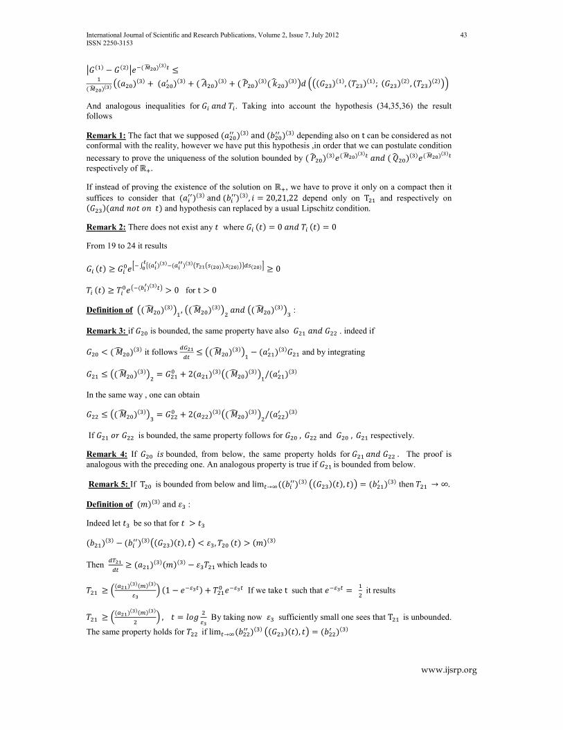
International Journal of Scientific and Research Publications, Volume 2, Issue 7, July 2012 43
ISSN 2250-3153
www.ijsrp.org
����� − �����;a� b�()����� ≤�� b�()���� ��������� + ����0 ���� + � Kc ������ + � jc������� c �������8 ����������, ��������; ��������, ����������
And analogous inequalities for �M �C8 �M . Taking into account the hypothesis (34,35,36) the result
follows
Remark 1: The fact that we supposed ����00 ���� and ����00 ���� depending also on t can be considered as not
conformal with the reality, however we have put this hypothesis ,in order that we can postulate condition
necessary to prove the uniqueness of the solution bounded by � jc������;� b�()����� �C8 � kc ������;� b�()�����
respectively of ℝ|. If instead of proving the existence of the solution on ℝ|, we have to prove it only on a compact then it
suffices to consider that ��M00���� and ��M00����, > = 20,21,22 depend only on T�� and respectively on �������C8 CD� DC �� and hypothesis can replaced by a usual Lipschitz condition.
Remark 2: There does not exist any � where �M ��� = 0 �C8 �M ��� = 0
From 19 to 24 it results
�M ��� ≥ �M�;"a ~ ��gh ����a�gh �����$(����()��,��()��¡���()��) # ≥ 0
�M ��� ≥ �M�;�a�ih ������ > 0 for t > 0
Definition of �� f���������, �� f��������� �C8 �� f��������� :
Remark 3: if ��� is bounded, the same property have also ��� �C8 ��� . indeed if
��� < � f������� it follows ��(��� ≤ �� f��������� − ����0 ������� and by integrating
��� ≤ �� f��������� = ���� + 2���������� f���������/����0 ���� In the same way , one can obtain
��� ≤ �� f��������� = ���� + 2���������� f���������/����0 ���� If ��� D< ��� is bounded, the same property follows for ��� , ��� and ��� , ��� respectively.
Remark 4: If ��� >? bounded, from below, the same property holds for ��� �C8 ��� . The proof is
analogous with the preceding one. An analogous property is true if ��� is bounded from below.
Remark 5: If T�� is bounded from below and lim�→Z���M00���� ���������, ��� = ����0 ���� then ��� → ∞. Definition of �B���� and ¤� :
Indeed let �� be so that for � > �� �������� − ��M00�������������, �� < ¤�, ��� ��� > �B����
Then �$(� �� ≥ ���������B���� − ¤���� which leads to
��� ≥ ��g(������¥����¦� � �1 − ;a¦��� + ���� ;a¦�� If we take t such that ;a¦�� = �� it results
��� ≥ ��g(������¥����� � , � = XDA �¦� By taking now ¤� sufficiently small one sees that T�� is unbounded.
The same property holds for ��� if lim�→Z����00 ���� ���������, �� = ����0 ����

International Journal of Scientific and Research Publications, Volume 2, Issue 7, July 2012 44
ISSN 2250-3153
www.ijsrp.org
We now state a more precise theorem about the behaviors at infinity of the solutions
It is now sufficient to take �gh�� �� bc( �� � , �ih�� �� bc( �� � < 1 and to choose
� Pc�� ���� and � Qc�� ���� large to have
�gh�� ��bc( �� � +� jc������ + �� jW�� ���� + ����;a�� �c( �� ����)��) �, ≤ � jW�� ����
�ih�� ��bc( �� � +�� kW�� ���� + ����;a� � �c( �� ����)��) � + � kW�� ����, ≤ � kW�� ����
In order that the operator y��� transforms the space of sextuples of functions �M , �M satisfying GLOBAL
EQUATIONS into itself
The operator y��� is a contraction with respect to the metric
8 ���������, ��������, ��������, ��������� =
?@Sh {B�J�∈ℝ� ��M������ − �M�������;a�bc( �� �� , B�J�∈ℝ� ��M������ − �M�������;a�bc( �� ��}
Indeed if we denote
Definition of ����² , ����² : � ����² , ����² � = y��������, �����
It results
�������� − ��M���� ≤ ~ ���������� ������� − �������;a� b�( �� ���( �;� b�( �� ���( � 8?���� +
~ {����0 ����������� − �������;a� b�( �� ���( �;a� b�( �� ���( ��� +
����00 �����������, ?������������ − �������;a� b�( �� ���( �;� b�( �� ���( � +
������|����00 �����������, ?����� − ����00 �����������, ?�����| ;a� b�( �� ���( �;� b�( �� ���( �}8?���� Where ?���� represents integrand that is integrated over the interval [0, t] From the hypotheses IT follows
�������� − ��������;a� b�( �� �� ≤�� b�( �� � ��������� + ����0 ���� + � Kc ������ + � jc������� c �������8 ���������, �������; �������, ���������
And analogous inequalities for �M �C8 �M . Taking into account the hypothesis (34,35,36) the result
follows
Remark 1: The fact that we supposed ����00 ���� and ����00 ���� depending also on t can be considered as not
conformal with the reality, however we have put this hypothesis ,in order that we can postulate condition
necessary to prove the uniqueness of the solution bounded by � jc������;� b�( �� �� �C8 � kc ������;� b�( �� ��

International Journal of Scientific and Research Publications, Volume 2, Issue 7, July 2012 45
ISSN 2250-3153
www.ijsrp.org
respectively of ℝ|. If instead of proving the existence of the solution on ℝ|, we have to prove it only on a compact then it
suffices to consider that ��M00���� and ��M00����, > = 24,25,26 depend only on T�� and respectively on ������C8 CD� DC �� and hypothesis can replaced by a usual Lipschitz condition.
Remark 2: There does not exist any � where �M ��� = 0 �C8 �M ��� = 0
From CONCATENATED GLOBAL EQUATIONS it results
�M ��� ≥ �M�;"a ~ ��gh �� �a�gh �� ��$(!���( ��,��( ��¡���( ��) # ≥ 0
�M ��� ≥ �M�;�a�ih �� ��� > 0 for t > 0
Definition of �� f���������, �� f��������� �C8 �� f��������� :
Remark 3: if ��� is bounded, the same property have also ��� �C8 ��� . indeed if
��� < � f������� it follows ��(!�� ≤ �� f��������� − ����0 ������� and by integrating
��� ≤ �� f��������� = ���� + 2���������� f���������/����0 ���� In the same way , one can obtain
��� ≤ �� f��������� = ���� + 2���������� f���������/����0 ���� If ��� D< ��� is bounded, the same property follows for ��� , ��� and ��� , ��� respectively.
Remark 4: If ��� >? bounded, from below, the same property holds for ��� �C8 ��� . The proof is
analogous with the preceding one. An analogous property is true if ��� is bounded from below.
Remark 5: If T�� is bounded from below and lim�→Z���M00���� ��������, ��� = ����0 ���� then ��� → ∞. Definition of �B���� and ¤� :
Indeed let �� be so that for � > �� �������� − ��M00������������, �� < ¤�, ��� ��� > �B����
Then �$(! �� ≥ ���������B���� − ¤���� which leads to
��� ≥ ��g(!�� ��¥�� �¦ � �1 − ;a¦ �� + ���� ;a¦ � If we take t such that ;a¦ � = �� it results
��� ≥ ��g(!�� ��¥�� �� � , � = XDA �¦ By taking now ¤� sufficiently small one sees that T�� is unbounded.
The same property holds for ��� if lim�→Z����00 ���� ��������, �� = ����0 ���� We now state a more precise theorem about the behaviors at infinity of the solutions
Analogous inequalities hold also for �� , ���, ��, �� , ���

International Journal of Scientific and Research Publications, Volume 2, Issue 7, July 2012 46
ISSN 2250-3153
www.ijsrp.org
It is now sufficient to take �gh��!�� bc(' ��!� , �ih��!�� bc(' ��!� < 1 and to choose
� Pc� ���� and � Qc� ���� large to have
�gh��!��bc('��!� +� jc����� + �� jW� ���� + ����;a�� �c(' ��!����)��) �, ≤ � jW� ����
�ih��!��bc('��!� +�� kW� ���� + ����;a� � �c(' ��!����)��) � + � kW� ����, ≤ � kW� ����
In order that the operator y��� transforms the space of sextuples of functions �M , �M satisfying GLOBAL
EQUATIONS into itself
The operator y��� is a contraction with respect to the metric
8 ����������, ���������, ���������, ���������� =
?@Sh {B�J�∈ℝ� ��M������ − �M�������;a�bc('��!�� , B�J�∈ℝ� ��M������ − �M�������;a�bc('��!��}
Indeed if we denote
Definition of �����² , �����² : � �����² , �����² � = y���������, ������
It results
������� − ��M���� ≤ ~ ��������� ��� ��� − �� ����;a� b�('��!���('�;� b�('��!���('� 8?��� +
~ {���0 ���������� − ������;a� b�('��!���('�;a� b�('��!���('��� +
���00 ������� ���, ?���������� − ������;a� b�('��!���('�;� b�('��!���('� +
�����|���00 ������� ���, ?���� − ���00 ������� ���, ?����| ;a� b�('��!���('�;� b�('��!���('�}8?��� Where ?��� represents integrand that is integrated over the interval [0, t] From the hypotheses it follows
��������� − ���������;a� b�('��!�� ≤�� b�('��!� �������� + ���0 ���� + � Kc ����� + � jc������ c ������8 ����������, ��������; ��������, ����������
And analogous inequalities for �M �C8 �M . Taking into account the hypothesis) the result follows
Remark 1: The fact that we supposed ���00 ���� and ���00 ���� depending also on t can be considered as not
conformal with the reality, however we have put this hypothesis ,in order that we can postulate condition
necessary to prove the uniqueness of the solution bounded by � jc�����;� b�('��!�� �C8 � kc �����;� b�('��!��
respectively of ℝ|.

International Journal of Scientific and Research Publications, Volume 2, Issue 7, July 2012 47
ISSN 2250-3153
www.ijsrp.org
If instead of proving the existence of the solution on ℝ|, we have to prove it only on a compact then it
suffices to consider that ��M00���� and ��M00����, > = 28,29,30 depend only on T� and respectively on �������C8 CD� DC �� and hypothesis can replaced by a usual Lipschitz condition.
Remark 2: There does not exist any � where �M ��� = 0 �C8 �M ��� = 0
From CONCATENATED EQUATIONS it results
�M ��� ≥ �M�;"a ~ ��gh ��!�a�gh ��!��$(*���('��,��('��¡���('��) # ≥ 0
�M ��� ≥ �M�;�a�ih ��!��� > 0 for t > 0
Definition of �� f��������, �� f�������� �C8 �� f�������� :
Remark 3: if �� is bounded, the same property have also �� �C8 ��� . indeed if
�� < � f������ it follows ��(*�� ≤ �� f�������� − ��� 0 ������ and by integrating
�� ≤ �� f�������� = �� � + 2��� ������ f��������/��� 0 ���� In the same way , one can obtain
��� ≤ �� f�������� = ���� + 2���������� f��������/����0 ���� If �� D< ��� is bounded, the same property follows for �� , ��� and �� , �� respectively.
Remark 4: If �� >? bounded, from below, the same property holds for �� �C8 ��� . The proof is
analogous with the preceding one. An analogous property is true if �� is bounded from below.
Remark 5: If T� is bounded from below and lim�→Z���M00���� ���������, ��� = ��� 0 ���� then �� → ∞. Definition of �B���� and ¤� :
Indeed let �� be so that for � > ��
��� ���� − ��M00�������������, �� < ¤�, �� ��� > �B����
Then �$(* �� ≥ ��� �����B���� − ¤��� which leads to
�� ≥ ��g(*��!��¥��!�¦! � �1 − ;a¦!�� + �� � ;a¦!� If we take t such that ;a¦!� = �� it results
�� ≥ ��g(*��!��¥��!�� � , � = XDA �¦! By taking now ¤� sufficiently small one sees that T� is unbounded.
The same property holds for ��� if lim�→Z����00 ���� ���������, �� = ����0 ���� We now state a more precise theorem about the behaviors at infinity of the solutions
Analogous inequalities hold also for ��� , ���, ���, ���, ���

International Journal of Scientific and Research Publications, Volume 2, Issue 7, July 2012 48
ISSN 2250-3153
www.ijsrp.org
It is now sufficient to take �gh��%�� bc�( ��%� , �ih��%�� bc�( ��%� < 1 and to choose
� Pc�� ���� and � Qc�� ���� large to have
�gh��%��bc�(��%� +� jc������ + �� jW�� ���� + ����;a�� �c�( ��%����)��) �, ≤ � jW�� ����
�ih��%��bc�(��%� +�� kW�� ���� + ����;a� � �c�( ��%����)��) � + � kW�� ����, ≤ � kW�� ����
In order that the operator y��� transforms the space of sextuples of functions �M , �M satisfying GLOBAL
EQUATIONS into itself
The operator y��� is a contraction with respect to the metric
8 ����������, ���������, ���������, ���������� =
?@Sh {B�J�∈ℝ� ��M������ − �M�������;a�bc�(��%�� , B�J�∈ℝ� ��M������ − �M�������;a�bc�(��%��}
Indeed if we denote
Definition of �����² , �����² : � �����² , �����² � = y���������, ������
It results
�������� − ��M���� ≤ ~ ���������� ������� − �������;a� b��(��%����(�;� b��(��%����(� 8?���� +
~ {����0 ����������� − �������;a� b��(��%����(�;a� b��(��%����(��� +
����00 �����������, ?������������ − �������;a� b��(��%����(�;� b��(��%����(� +
������|����00 �����������, ?����� − ����00 �����������, ?�����| ;a� b��(��%����(�;� b��(��%����(�}8?���� Where ?���� represents integrand that is integrated over the interval [0, t] From the hypotheses it follows
��������� − ���������;a� b��(��%�� ≤�� b��(��%� ��������� + ����0 ���� + � Kc ������ + � jc������� c �������8 ����������, ��������; ��������, ����������
And analogous inequalities for �M �C8 �M . Taking into account the hypothesis the result follows
Remark 1: The fact that we supposed ����00 ���� and ����00 ���� depending also on t can be considered as not
conformal with the reality, however we have put this hypothesis ,in order that we can postulate condition
necessary to prove the uniqueness of the solution bounded by � jc������;� b��(��%�� �C8 � kc �������� b��(��%��
respectively of ℝ|. If instead of proving the existence of the solution on ℝ|, we have to prove it only on a compact then it
suffices to consider that ��M00���� and ��M00����, > = 32,33,34 depend only on T�� and respectively on

International Journal of Scientific and Research Publications, Volume 2, Issue 7, July 2012 49
ISSN 2250-3153
www.ijsrp.org
�������C8 CD� DC �� and hypothesis can replaced by a usual Lipschitz condition.
Remark 2: There does not exist any � where �M ��� = 0 �C8 �M ��� = 0
From 69 to 32 it results
�M ��� ≥ �M�;"a ~ ��gh ��%�a�gh ��%��$������(��,���(��¡����(��) # ≥ 0
�M ��� ≥ �M�;�a�ih ��%��� > 0 for t > 0
Definition of �� f���������, �� f��������� �C8 �� f��������� :
Remark 3: if ��� is bounded, the same property have also ��� �C8 ��� . indeed if
��� < � f������� it follows ������ ≤ �� f��������� − ����0 ������� and by integrating
��� ≤ �� f��������� = ���� + 2���������� f���������/����0 ���� In the same way , one can obtain
��� ≤ �� f��������� = ���� + 2���������� f���������/����0 ���� If ��� D< ��� is bounded, the same property follows for ��� , ��� and ��� , ��� respectively.
Remark 4: If ��� >? bounded, from below, the same property holds for ��� �C8 ��� . The proof is
analogous with the preceding one. An analogous property is true if ��� is bounded from below.
Remark 5: If T�� is bounded from below and lim�→Z���M00���� ���������, ��� = ����0 ���� then ��� → ∞. Definition of �B���� and ¤� :
Indeed let �� be so that for � > ��
�������� − ��M00�������������, �� < ¤�, ��� ��� > �B����
Then �$�� �� ≥ ���������B���� − ¤���� which leads to
��� ≥ ��g����%��¥��%�¦% � �1 − ;a¦%�� + ���� ;a¦%� If we take t such that ;a¦%� = �� it results
��� ≥ ��g����%��¥��%�� � , � = XDA �¦% By taking now ¤� sufficiently small one sees that T�� is unbounded.
The same property holds for ��� if lim�→Z����00 ���� ���������, ����, �� = ����0 ���� We now state a more precise theorem about the behaviors at infinity of the solutions
Behavior of the solutions
Theorem 2: If we denote and define
Definition of �³����� , �³����� , �´����� , �´����� :

International Journal of Scientific and Research Publications, Volume 2, Issue 7, July 2012 50
ISSN 2250-3153
www.ijsrp.org
(a) ³����� , �³����� , �´����� , �´����� four constants satisfying
−�³����� ≤ −����0 ���� + ����0 ���� − ����00 �������� , �� + ����00 �������� , �� ≤ −�³����� −�´����� ≤ −����0 ���� + ����0 ���� − ����00 ������, �� − ����00 ������, �� ≤ −�´����� Definition of �µ�����, �µ�����, �@�����, �@�����, µ���, @��� : (b) By �µ����� > 0 , �µ����� < 0 and respectively �@����� > 0 , �@����� < 0 the roots of the equations ���������µ����� + �³�����µ��� − �������� = 0 and ���������@����� + �´�����@��� − �������� = 0
Definition of �µ}�����, , �µ}�����, �@������, �@������ : By �µ}����� > 0 , �µ}����� < 0 and respectively �@������ > 0 , �@������ < 0 the roots of the equations ���������µ����� + �³�����µ��� − �������� = 0 and ���������@����� + �´�����@��� − �������� = 0
Definition of �B����� , �B����� , �¶�����, �¶�����, �µ����� :- (c) If we define �B����� , �B����� , �¶�����, �¶����� by
�B����� = �µ�����, �B����� = �µ�����, >= �µ����� < �µ����� �B����� = �µ�����, �B����� = �µ}����� , >= �µ����� < �µ����� < �µ}�����, and �µ����� = ���)�� )
� B����� = �µ�����, �B����� = �µ�����, >= �µ}����� < �µ�����
and analogously
�¶����� = �@�����, �¶����� = �@�����, >= �@����� < �@����� �¶����� = �@�����, �¶����� = �@������ , >= �@����� < �@����� < �@������, and �@����� = $��)$� )
� ¶����� = �@�����, �¶����� = �@�����, >= �@������ < �@����� where �@�����, �@������ are defined respectively
Then the solution of GLOBAL EQUATSIONS satisfies the inequalities
���� ;��·�����a�¸�������� ≤ ������ ≤ ���� ;�·������
where �SM���� is defined by equation 25
� �¥����� ���� ;��·�����a�¸�������� ≤ ������ ≤ ��¥(���� ���� ;�·������
� �g�!�������)�¥�������·�����a�¸������a�·(����� ";��·�����a�¸�������� − ;a�·(����� # + ���� ;a�·(����� ≤ ������ ≤�g�!�������)�¥(������·�����a�g�! ����� [;�·������ − ;a�g�! �����] + ���� ;a�g�! ������
���� ;�¹������ ≤ ������ ≤ ���� ;��¹�����|�º��������
��»����� ���� ;�¹������ ≤ ������ ≤ ��»(���� ���� ;��¹�����|�º��������

International Journal of Scientific and Research Publications, Volume 2, Issue 7, July 2012 51
ISSN 2250-3153
www.ijsrp.org
�i�!����$��)�»�������¹�����a�i�! ����� ";�¹������ − ;a�i�! �����# + ���� ;a�i�! ����� ≤ ������ ≤
�g�!����$��)�»(������¹�����|�º������|�¹(����� ";��¹�����|�º�������� − ;a�¹(�����# + ���� ;a�¹(�����
Definition of �¼�����, �¼�����, �½�����, �½�����:- Where �¼����� = ���������B����� − ����0 ���� �¼����� = �������� − �S������ �½����� = ���������¶����� − ����0 ���� �½����� = ����0 ���� − �<������
If we denote and define
Definition of ���� , ���� , ���� , ���� : (d) ��� , ���� , ���� , ���� four constants satisfying
−�σ����� ≤ −����0 ���� + ���0 ���� − ����00 �����T� , �� + ���00 �����T� , �� ≤ −�σ�����
−�τ����� ≤ −����0 ���� + ���0 ���� − ����00 �������� �, �� − ���00 �������� �, �� ≤ −�τ�����
Definition of �µ�����, �ν�����, �@�����, �@����� :
By �µ����� > 0 , �ν����� < 0 and respectively �@����� > 0 , �@����� < 0 the roots
(e) of the equations ��������µ����� + �σ�����µ��� − �������� = 0
and ���������@����� + �τ�����@��� − �������� = 0 and
Definition of �µ}�����, , �µ}�����, �@������, �@������ :
By �µ}����� > 0 , �ν������ < 0 and respectively �@������ > 0 , �@������ < 0 the
roots of the equations ��������µ����� + �σ�����µ��� − �������� = 0
and ��������@����� + �τ�����@��� − �������� = 0
Definition of �B����� , �B����� , �¶�����, �¶����� :-
(f) If we define �B����� , �B����� , �¶�����, �¶����� by
�B����� = �µ�����, �B����� = �µ�����, Á �µ����� < �µ�����
�B����� = �µ�����, �B����� = �µ}����� , Á �µ����� < �µ����� < �µ}�����, and �µ����� = ^�%)^�&)
� B����� = �µ�����, �B����� = �µ�����, Á �µ}����� < �µ�����
and analogously

International Journal of Scientific and Research Publications, Volume 2, Issue 7, July 2012 52
ISSN 2250-3153
www.ijsrp.org
�¶����� = �@�����, �¶����� = �@�����, Á �@����� < �@����� �¶����� = �@�����, �¶����� = �@������ , Á �@����� < �@����� < �@������, and �@����� = ª�%)ª�&)
� ¶����� = �@�����, �¶����� = �@�����, Á �@������ < �@�����
Then the solution of HOLISTIC GLOBAL EQUATIONS satisfies the inequalities
G��� e��Ã���(�a�¸�%��(��¨ ≤ ������ ≤ G��� e�Ã���(�¨
�SM���� is defined by equation 25
� �¥���(� G��� e��Ã���(�a�¸�%��(��¨ ≤ ����� ≤ ��¥(��(� G��� e�Ã���(�¨
� �g�'��(�^�%)�¥���(���Ã���(�a�¸�%��(�a�Ã(��(�� "e��Ã���(�a�¸�%��(��¨ − ea�Ã(��(�¨ # + G�� ea�Ã(��(�¨ ≤ G���� ≤�g�'��(�^�%)�¥(��(���Ã���(�a�g�' ��(�� [e�Ã���(�¨ − ea�g�' ��(�¨] + G�� ea�g�' ��(�¨�
T��� e�Ä���(�� ≤ ������ ≤ T��� e��Ä���(�|�º�%��(���
��»���(� T��� e�Ä���(�� ≤ ������ ≤ ��»(��(� T��� e��Ä���(�|�º�%��(���
�i�'��(�ª�%)�»���(���Ä���(�a�i�' ��(�� "e�Ä���(�� − ea�i�' ��(��# + T�� ea�i�' ��(�� ≤ ����� ≤
�g�'��(�ª�%)�»(��(���Ä���(�|�º�%��(�|�Ä(��(�� "e��Ä���(�|�º�%��(��� − ea�Ä(��(��# + T�� ea�Ä(��(��
Definition of �S�����, �S�����, �R�����, �R�����:-
Where �S����� = ���������B����� − ����0 ���� �S����� = ������� − �S�����
�½����� = ���������¶����� − ����0 ���� �R����� = ���0 ���� − �<�����
Behavior of the solutions
If we denote and define
Definition of �³����� , �³����� , �´����� , �´����� : (a) ³����� , �³����� , �´����� , �´����� four constants satisfying
−�³����� ≤ −����0 ���� + ����0 ���� − ����00 �������� , �� + ����00 �������� , �� ≤ −�³����� −�´����� ≤ −����0 ���� + ����0 ���� − ����00 ������, �� − ����00 ����������, �� ≤ −�´�����
Definition of �µ�����, �µ�����, �@�����, �@����� : (b) By �µ����� > 0 , �µ����� < 0 and respectively �@����� > 0 , �@����� < 0 the roots of the equations

International Journal of Scientific and Research Publications, Volume 2, Issue 7, July 2012 53
ISSN 2250-3153
www.ijsrp.org
���������µ����� + �³�����µ��� − �������� = 0
and ���������@����� + �´�����@��� − �������� = 0 and
By �µ}����� > 0 , �µ}����� < 0 and respectively �@������ > 0 , �@������ < 0 the
roots of the equations ���������µ����� + �³�����µ��� − �������� = 0
and ���������@����� + �´�����@��� − �������� = 0
Definition of �B����� , �B����� , �¶�����, �¶����� :- (c) If we define �B����� , �B����� , �¶�����, �¶����� by
�B����� = �µ�����, �B����� = �µ�����, Á �µ����� < �µ����� �B����� = �µ�����, �B����� = �µ}����� , Á �µ����� < �µ����� < �µ}�����, and �µ����� = �())�(�)
� B����� = �µ�����, �B����� = �µ�����, Á �µ}����� < �µ�����
and analogously
�¶����� = �@�����, �¶����� = �@�����, Á �@����� < �@����� �¶����� = �@�����, �¶����� = �@������ , Á �@����� < �@����� < �@������, and �@����� = $())$(�)
� ¶����� = �@�����, �¶����� = �@�����, Á �@������ < �@����� Then the solution of GLOBAL EQUATIONS satisfies the inequalities
���� ;��·�����a�¸()������ ≤ ������ ≤ ���� ;�·������
�SM���� is defined
� �¥����� ���� ;��·�����a�¸()������ ≤ ������ ≤ ��¥(���� ���� ;�·������
� �g((�����())�¥�������·�����a�¸()����a�·(����� ";��·�����a�¸()������ − ;a�·(����� # + ���� ;a�·(����� ≤ ������ ≤�g((�����())�¥(������·�����a�g(( ����� [;�·������ − ;a�g(( �����] + ���� ;a�g(( ������
���� ;�¹������ ≤ ������ ≤ ���� ;��¹�����|�º()������
��»����� ���� ;�¹������ ≤ ������ ≤ ��»(���� ���� ;��¹�����|�º()������
�i((����$())�»�������¹�����a�i(( ����� ";�¹������ − ;a�i(( �����# + ���� ;a�i(( ����� ≤ ������ ≤
�g((����$())�»(������¹�����|�º()����|�¹(����� ";��¹�����|�º()������ − ;a�¹(�����# + ���� ;a�¹(�����
Definition of �¼�����, �¼�����, �½�����, �½�����:- Where �¼����� = ���������B����� − ����0 ����

International Journal of Scientific and Research Publications, Volume 2, Issue 7, July 2012 54
ISSN 2250-3153
www.ijsrp.org
�¼����� = �������� − �S������ �½����� = ���������¶����� − ����0 ����
�½����� = ����0 ���� − �<������
Behavior of the solutions
Theorem 2: If we denote and define
Definition of �³����� , �³����� , �´����� , �´����� :
(d) �³����� , �³����� , �´����� , �´����� four constants satisfying
−�³����� ≤ −����0 ���� + ����0 ���� − ����00 �������� , �� + ����00 �������� , �� ≤ −�³����� −�´����� ≤ −����0 ���� + ����0 ���� − ����00 ���������, �� − ����00 ���������, �� ≤ −�´�����
Definition of �µ�����, �µ�����, �@�����, �@�����, µ���, @��� :
(e) By �µ����� > 0 , �µ����� < 0 and respectively �@����� > 0 , �@����� < 0 the roots of the
equations ���������µ����� + �³�����µ��� − �������� = 0
and ���������@����� + �´�����@��� − �������� = 0 and
Definition of �µ}�����, , �µ}�����, �@������, �@������ :
By �µ}����� > 0 , �µ}����� < 0 and respectively �@������ > 0 , �@������ < 0 the
roots of the equations ���������µ����� + �³�����µ��� − �������� = 0
and ���������@����� + �´�����@��� − �������� = 0
Definition of �B����� , �B����� , �¶�����, �¶�����, �µ����� :-
(f) If we define �B����� , �B����� , �¶�����, �¶����� by
�B����� = �µ�����, �B����� = �µ�����, Á �µ����� < �µ�����
�B����� = �µ�����, �B����� = �µ}����� , Á �µ����� < �µ����� < �µ}�����, and �µ����� = �( )�(!)
� B����� = �µ�����, �B����� = �µ�����, Á �µ}����� < �µ�����
and analogously
�¶����� = �@�����, �¶����� = �@�����, Á �@����� < �@�����
�¶����� = �@�����, �¶����� = �@������ , Á �@����� < �@����� < �@������, and �@����� = $( )$(!)
� ¶����� = �@�����, �¶����� = �@�����, Á �@������ < �@����� where �@�����, �@������ are defined by 59 and 64 respectively
Then the solution of 19,20,21,22,23 and 24 satisfies the inequalities

International Journal of Scientific and Research Publications, Volume 2, Issue 7, July 2012 55
ISSN 2250-3153
www.ijsrp.org
���� ;��·��� �a�¸( �� ��� ≤ ������ ≤ ���� ;�·��� ��
where �SM���� is defined by equation 25
� �¥��� � ���� ;��·��� �a�¸( �� ��� ≤ ������ ≤ ��¥(�� � ���� ;�·��� ��
Ç �g(%�� ��( )�¥��� ���·��� �a�¸( �� �a�·(�� �� ";��·��� �a�¸( �� ��� − ;a�·(�� �� # + ���� ;a�·(�� �� ≤ ������ ≤��26�4�240�B2�4�¼1�4−��26′�4;�¼1�4�−;−��26′�4�+ �260;−��26′�4�
���� ;�¹��� �� ≤ ������ ≤ ���� ;��¹��� �|�º( �� ���
��»��� � ���� ;�¹��� �� ≤ ������ ≤ ��»(�� � ���� ;��¹��� �|�º( �� ���
�i(%�� �$( )�»��� ���¹��� �a�i(% �� �� ";�¹��� �� − ;a�i(% �� ��# + ���� ;a�i(% �� �� ≤ ������ ≤
�g(%�� �$( )�»(�� ���¹��� �|�º( �� �|�¹(�� �� ";��¹��� �|�º( �� ��� − ;a�¹(�� ��# + ���� ;a�¹(�� ��
Definition of �¼�����, �¼�����, �½�����, �½�����:-
Where �¼����� = ���������B����� − ����0 ���� �¼����� = �������� − �S������
�½����� = ���������¶����� − ����0 ����
�½����� = ����0 ���� − �<������
Behavior of the solutions of equation 37 to 42
Theorem 2: If we denote and define
Definition of �³����� , �³����� , �´����� , �´����� :
(g) �³����� , �³����� , �´����� , �´����� four constants satisfying
−�³����� ≤ −���0 ���� + ��� 0 ���� − ���00 ������� , �� + ��� 00 ������� , �� ≤ −�³����� −�´����� ≤ −���0 ���� + ��� 0 ���� − ���00 ����������, �� − ��� 00 ����������, �� ≤ −�´�����
Definition of �µ�����, �µ�����, �@�����, �@�����, µ���, @��� :
(h) By �µ����� > 0 , �µ����� < 0 and respectively �@����� > 0 , �@����� < 0 the roots of the
equations ��� �����µ����� + �³�����µ��� − ������� = 0
and ��� �����@����� + �´�����@��� − ������� = 0 and
Definition of �µ}�����, , �µ}�����, �@������, �@������ :
By �µ}����� > 0 , �µ}����� < 0 and respectively �@������ > 0 , �@������ < 0 the
roots of the equations ��� �����µ����� + �³�����µ��� − ������� = 0

International Journal of Scientific and Research Publications, Volume 2, Issue 7, July 2012 56
ISSN 2250-3153
www.ijsrp.org
and ��� �����@����� + �´�����@��� − ������� = 0
Definition of �B����� , �B����� , �¶�����, �¶�����, �µ����� :-
(i) If we define �B����� , �B����� , �¶�����, �¶����� by
�B����� = �µ�����, �B����� = �µ�����, Á �µ����� < �µ�����
�B����� = �µ�����, �B����� = �µ}����� , Á �µ����� < �µ����� < �µ}�����, and �µ����� = �(')�(*)
� B����� = �µ�����, �B����� = �µ�����, Á �µ}����� < �µ����� and analogously
�¶����� = �@�����, �¶����� = �@�����, Á �@����� < �@�����
�¶����� = �@�����, �¶����� = �@������ , Á �@����� < �@����� < �@������, and �@����� = $(')$(*)
� ¶����� = �@�����, �¶����� = �@�����, Á �@������ < �@����� where �@�����, �@������ are defined by 59 and 65 respectively
Then the solution of 19,20,21,22,23 and 24 satisfies the inequalities
��� ;��·���!�a�¸('��!��� ≤ ����� ≤ ��� ;�·���!��
where �SM���� is defined by equation 29
� �¥!��!� ��� ;��·���!�a�¸('��!��� ≤ �� ��� ≤ ��¥(��!� ��� ;�·���!��
Ç �g�)��!��(')�¥���!���·���!�a�¸('��!�a�·(��!�� ";��·���!�a�¸('��!��� − ;a�·(��!�� # + ���� ;a�·(��!�� ≤ ������ ≤��30�5�280�B2�5�¼1�5−��30′�5;�¼1�5�−;−��30′�5�+ �300;−��30′�5�
��� ;�¹���!�� ≤ ����� ≤ ��� ;��¹���!�|�º('��!���
��»���!� ��� ;�¹���!�� ≤ ����� ≤ ��»(��!� ��� ;��¹���!�|�º('��!���
�i�)��!�$(')�»���!���¹���!�a�i�) ��!�� ";�¹���!�� − ;a�i�) ��!��# + ���� ;a�i�) ��!�� ≤ ������ ≤
�g�)��!�$(')�»(��!���¹���!�|�º('��!�|�¹(��!�� ";��¹���!�|�º('��!��� − ;a�¹(��!��# + ���� ;a�¹(��!��
Definition of �¼�����, �¼�����, �½�����, �½�����:-
Where �¼����� = ��������B����� − ���0 ���� �¼����� = �������� − �S������
�½����� = ��������¶����� − ���0 ����
�½����� = ����0 ���� − �<������

International Journal of Scientific and Research Publications, Volume 2, Issue 7, July 2012 57
ISSN 2250-3153
www.ijsrp.org
Behavior of the solutions of equation 37 to 42
Theorem 2: If we denote and define
Definition of �³����� , �³����� , �´����� , �´����� :
(j) �³����� , �³����� , �´����� , �´����� four constants satisfying
−�³����� ≤ −����0 ���� + ����0 ���� − ����00 �������� , �� + ����00 �������� , �� ≤ −�³����� −�´����� ≤ −����0 ���� + ����0 ���� − ����00 ����������, �� − ����00 ����������, �� ≤ −�´�����
Definition of �µ�����, �µ�����, �@�����, �@�����, µ���, @��� :
(k) By �µ����� > 0 , �µ����� < 0 and respectively �@����� > 0 , �@����� < 0 the roots of the
equations ���������µ����� + �³�����µ��� − �������� = 0
and ���������@����� + �´�����@��� − �������� = 0 and
Definition of �µ}�����, , �µ}�����, �@������, �@������ :
By �µ}����� > 0 , �µ}����� < 0 and respectively �@������ > 0 , �@������ < 0 the
roots of the equations ���������µ����� + �³�����µ��� − �������� = 0
and ���������@����� + �´�����@��� − �������� = 0
Definition of �B����� , �B����� , �¶�����, �¶�����, �µ����� :-
(l) If we define �B����� , �B����� , �¶�����, �¶����� by
�B����� = �µ�����, �B����� = �µ�����, Á �µ����� < �µ�����
�B����� = �µ�����, �B����� = �µ}����� , Á �µ����� < �µ����� < �µ}�����, and �µ����� = ��()���)
� B����� = �µ�����, �B����� = �µ�����, Á �µ}����� < �µ�����
and analogously
�¶����� = �@�����, �¶����� = �@�����, Á �@����� < �@�����
�¶����� = �@�����, �¶����� = �@������ , Á �@����� < �@����� < �@������, and �@����� = $�()$��)
� ¶����� = �@�����, �¶����� = �@�����, Á �@������ < �@����� where �@�����, �@������ are defined by 59 and 66 respectively
Then the solution of 19,20,21,22,23 and 24 satisfies the inequalities
���� ;��·���%�a�¸�(��%��� ≤ ������ ≤ ���� ;�·���%��
where �SM���� is defined by equation 25
� �¥���%� ���� ;��·���%�a�¸�(��%��� ≤ ������ ≤ ��¥(��%� ���� ;�·���%��

International Journal of Scientific and Research Publications, Volume 2, Issue 7, July 2012 58
ISSN 2250-3153
www.ijsrp.org
Ç �g� ��%���()�¥���%���·���%�a�¸�(��%�a�·(��%�� ";��·���%�a�¸�(��%��� − ;a�·(��%�� # + ���� ;a�·(��%�� ≤ ������ ≤��34�6�320�B2�6�¼1�6−��34′�6;�¼1�6�−;−��34′�6�+ �340;−��34′�6�
���� ;�¹���%�� ≤ ������ ≤ ���� ;��¹���%�|�º�(��%���
��»���%� ���� ;�¹���%�� ≤ ������ ≤ ��»(��%� ���� ;��¹���%�|�º�(��%���
�i� ��%�$�()�»���%���¹���%�a�i� ��%�� ";�¹���%�� − ;a�i� ��%��# + ���� ;a�i� ��%�� ≤ ������ ≤
�g� ��%�$�()�»(��%���¹���%�|�º�(��%�|�¹(��%�� ";��¹���%�|�º�(��%��� − ;a�¹(��%��# + ���� ;a�¹(��%��
Definition of �¼�����, �¼�����, �½�����, �½�����:-
Where �¼����� = ���������B����� − ����0 ���� �¼����� = �������� − �S������
�½����� = ���������¶����� − ����0 ����
�½����� = ����0 ���� − �<������
Proof : From 19,20,21,22,23,24 we obtain
�É����� = �������� − �����0 ���� − ����0 ���� + ����00 ��������, ��� − ����00 ��������, ��µ��� − ��������µ��� Definition of µ��� :- µ��� = �����
It follows
− ����������µ����� + �³�����µ��� − ��������� ≤ �É����� ≤ − ����������µ����� + �³�����µ��� − ���������
From which one obtains
Definition of �µ}�����, �µ����� :-
(a) For 0 < �µ����� = ���)�� ) < �µ����� < �µ}�����
µ������ ≥ �É�����|�Ê�����É(����Ë"Ì�Í� ������Î�����Ì�Î)����� �#�|�Ê����Ë"Ì�Í� ������Î�����Ì�Î)����� �# , �Ï���� = �É�����a�É)�����É)����a�É(����
it follows �µ����� ≤ µ������ ≤ �µ�����
In the same manner , we get
µ������ ≤ �É������|�Ê}�����É�(����Ë"Ì�Í� ������Î������Ì�Î�(����� �#�|�Ê}����Ë"Ì�Í� ������Î������Ì�Î�(����� �# , �Ï}���� = �É������a�É)�����É)����a�É�(����

International Journal of Scientific and Research Publications, Volume 2, Issue 7, July 2012 59
ISSN 2250-3153
www.ijsrp.org
From which we deduce �µ����� ≤ µ������ ≤ �µ}�����
(b) If 0 < �µ����� < �µ����� = ���)�� ) < �µ}����� we find like in the previous case,
�µ����� ≤ �É�����|�Ê�����É(����Ë"Ì�Í� ������Î�����Ì�Î(����� �#�|�Ê����Ë"Ì�Í� ������Î�����Ì�Î(����� �# ≤ µ������ ≤
�É������|�Ê}�����É�(����Ë"Ì�Í� ������Î������Ì�Î�(����� �#�|�Ê}����Ë"Ì�Í� ������Î������Ì�Î�(����� �# ≤ �µ}�����
(c) If 0 < �µ����� ≤ �µ}����� ≤ �µ����� = ���)�� ) , we obtain
�µ����� ≤ µ������ ≤ �É������|�Ê}�����É�(����Ë"Ì�Í� ������Î������Ì�Î�(����� �#�|�Ê}����Ë"Ì�Í� ������Î������Ì�Î�(����� �# ≤ �µ�����
And so with the notation of the first part of condition (c) , we have
Definition of µ������ :-
�B����� ≤ µ������ ≤ �B�����, µ������ = �������� ���
In a completely analogous way, we obtain
Definition of @������ :- �¶����� ≤ @������ ≤ �¶�����, @������ = $�����$� ���
Now, using this result and replacing it in 19, 20,21,22,23, and 24 we get easily the result stated in the
theorem.
Particular case :
If ����00 ���� = ����00 ����, �ℎ;C �³����� = �³����� and in this case �µ����� = �µ}����� if in addition �µ����� =�µ����� then µ������ = �µ����� and as a consequence ������ = �µ����������� this also defines �µ����� for the
special case
Analogously if ����00 ���� = ����00 ����, �ℎ;C �´����� = �´����� and then
�@����� = �@������if in addition �@����� = �@����� then ������ = �@����������� This is an important
consequence of the relation between �µ����� and �µ}�����, and definition of �@�����.
Proof : From 19,20,21,22,23,24 we obtain
«É�(�«¨ = �������� − �����0 ���� − ���0 ���� + ����00 �����T�, t�� − ���00 �����T�, t�µ��� − �������µ���
Definition of µ��� :- µ��� = ^�%^�&
It follows

International Journal of Scientific and Research Publications, Volume 2, Issue 7, July 2012 60
ISSN 2250-3153
www.ijsrp.org
− ���������µ����� + �σ�����µ��� − ��������� ≤ «É�(�«¨ ≤ − ���������µ����� + �σ�����µ��� − ��������� From which one obtains
Definition of �µ}�����, �µ����� :- (d) For 0 < �µ����� = ^�%)^�&) < �µ����� < �µ}�����
µ������ ≥ �É���(�|�Ñ��(��É(��(�Ë"Ì�Í�&��(���Î���(�Ì�Î)��(�� �#�|�Ñ��(�Ë"Ì�Í�&��(���Î���(�Ì�Î)��(�� �# , �C���� = �É���(�a�É)��(��É)��(�a�É(��(�
it follows �µ����� ≤ µ������ ≤ �µ�����
In the same manner , we get
µ������ ≤ �É����(�|�Ñ���(��É�(��(�Ë"Ì�Í�&��(���Î����(�Ì�Î�(��(�� �#�|�Ñ���(�Ë"Ì�Í�&��(���Î����(�Ì�Î�(��(�� �# , �C����� = �É����(�a�É)��(��É)��(�a�É�(��(�
From which we deduce �µ����� ≤ µ������ ≤ �µ}�����
(e) If 0 < �µ����� < �µ����� = ^�%)^�&) < �µ}����� we find like in the previous case,
�µ����� ≤ �É���(�|�Ñ��(��É(��(�Ë"Ì�Í�&��(���Î���(�Ì�Î(��(�� �#�|�Ñ��(�Ë"Ì�Í�&��(���Î���(�Ì�Î(��(�� �# ≤ µ������ ≤
�É����(�|�Ñ���(��É�(��(�Ë"Ì�Í�&��(���Î����(�Ì�Î�(��(�� �#�|�Ñ���(�Ë"Ì�Í�&��(���Î����(�Ì�Î�(��(�� �# ≤ �µ}�����
(f) If 0 < �µ����� ≤ �µ}����� ≤ �µ����� = ^�%)^�&) , we obtain
�µ����� ≤ µ������ ≤ �É����(�|�Ñ���(��É�(��(�Ë"Ì�Í�&��(���Î����(�Ì�Î�(��(�� �#�|�Ñ���(�Ë"Ì�Í�&��(���Î����(�Ì�Î�(��(�� �# ≤ �µ�����
And so with the notation of the first part of condition (c) , we have
Definition of µ������ :-
�B����� ≤ µ������ ≤ �B�����, µ������ = ��%�����&���
In a completely analogous way, we obtain
Definition of @������ :- �¶����� ≤ @������ ≤ �¶�����, @������ = $�%���$�&���
Now, using this result and replacing it in 19, 20,21,22,23, and 24 we get easily the result stated in the
theorem.
Particular case :
If ����00 ���� = ���00 ����, �ℎ;C �σ����� = �σ����� and in this case �µ����� = �µ}����� if in addition �µ����� =�µ����� then µ������ = �µ����� and as a consequence ������ = �µ����������

International Journal of Scientific and Research Publications, Volume 2, Issue 7, July 2012 61
ISSN 2250-3153
www.ijsrp.org
Analogously if ����00 ���� = ���00 ����, �ℎ;C �τ����� = �τ����� and then
�@����� = �@������if in addition �@����� = �@����� then ������ = �@���������� This is an important
consequence of the relation between �µ����� and �µ}�����
Proof : From 19,20,21,22,23,24 we obtain
�É����� = �������� − �����0 ���� − ����0 ���� + ����00 ��������, ��� − ����00 ��������, ��µ��� − ��������µ���
Definition of µ��� :- µ��� = �()�(�
It follows
− ����������µ����� + �³�����µ��� − ��������� ≤ �É����� ≤ − ����������µ����� + �³�����µ��� − ���������
From which one obtains
(a) For 0 < �µ����� = �())�(�) < �µ����� < �µ}�����
µ������ ≥ �É�����|�Ê�����É(����Ë"Ì�Í(�������Î�����Ì�Î)����� �#�|�Ê����Ë"Ì�Í(�������Î�����Ì�Î)����� �# , �Ï���� = �É�����a�É)�����É)����a�É(����
it follows �µ����� ≤ µ������ ≤ �µ�����
In the same manner , we get
µ������ ≤ �É������|�Ê}�����É�(����Ë"Ì�Í(�������Î������Ì�Î�(����� �#�|�Ê}����Ë"Ì�Í(�������Î������Ì�Î�(����� �# , �Ï}���� = �É������a�É)�����É)����a�É�(����
Definition of �µ}����� :- From which we deduce �µ����� ≤ µ������ ≤ �µ}�����
(b) If 0 < �µ����� < �µ����� = �())�(�) < �µ}����� we find like in the previous case,
�µ����� ≤ �É�����|�Ê�����É(����Ë"Ì�Í(�������Î�����Ì�Î(����� �#�|�Ê����Ë"Ì�Í(�������Î�����Ì�Î(����� �# ≤ µ������ ≤
�É������|�Ê}�����É�(����Ë"Ì�Í(�������Î������Ì�Î�(����� �#�|�Ê}����Ë"Ì�Í(�������Î������Ì�Î�(����� �# ≤ �µ}�����
(c) If 0 < �µ����� ≤ �µ}����� ≤ �µ����� = �())�(�) , we obtain
�µ����� ≤ µ������ ≤ �É������|�Ê}�����É�(����Ë"Ì�Í(�������Î������Ì�Î�(����� �#�|�Ê}����Ë"Ì�Í(�������Î������Ì�Î�(����� �# ≤ �µ�����
And so with the notation of the first part of condition (c) , we have

International Journal of Scientific and Research Publications, Volume 2, Issue 7, July 2012 62
ISSN 2250-3153
www.ijsrp.org
Definition of µ������ :-
�B����� ≤ µ������ ≤ �B�����, µ������ = �()����(����
In a completely analogous way, we obtain
Definition of @������ :- �¶����� ≤ @������ ≤ �¶�����, @������ = $()���$(����
Now, using this result and replacing it in 19, 20,21,22,23, and 24 we get easily the result stated in the
theorem.
Particular case :
If ����00 ���� = ����00 ����, �ℎ;C �³����� = �³����� and in this case �µ����� = �µ}����� if in addition �µ����� =�µ����� then µ������ = �µ����� and as a consequence ������ = �µ�����������
Analogously if ����00 ���� = ����00 ����, �ℎ;C �´����� = �´����� and then
�@����� = �@������if in addition �@����� = �@����� then ������ = �@����������� This is an important
consequence of the relation between �µ����� and �µ}�����
Proof : From 19,20,21,22,23,24 we obtain
�É� ��� = �������� − �����0 ���� − ����0 ���� + ����00 ��������, ��� − ����00 ��������, ��µ��� − ��������µ���
Definition of µ��� :- µ��� = �( �(!
It follows
− ����������µ����� + �³�����µ��� − ��������� ≤ �É� ��� ≤ − ����������µ����� + �³�����µ��� − ���������
From which one obtains
Definition of �µ}�����, �µ����� :-
(d) For 0 < �µ����� = �( )�(!) < �µ����� < �µ}�����
µ������ ≥ �É��� �|�Ê�� ��É(�� �Ë"Ì�Í(!�� ���Î��� �Ì�Î)�� �� �#�|�Ê�� �Ë"Ì�Í(!�� ���Î��� �Ì�Î)�� �� �# , �Ï���� = �É��� �a�É)�� ��É)�� �a�É(�� �
it follows �µ����� ≤ µ������ ≤ �µ�����
In the same manner , we get
µ������ ≤ �É���� �|�Ê}�� ��É�(�� �Ë"Ì�Í(!�� ���Î���� �Ì�Î�(�� �� �#�|�Ê}�� �Ë"Ì�Í(!�� ���Î���� �Ì�Î�(�� �� �# , �Ï}���� = �É���� �a�É)�� ��É)�� �a�É�(�� �
From which we deduce �µ����� ≤ µ������ ≤ �µ}�����
(e) If 0 < �µ����� < �µ����� = �( )�(!) < �µ}����� we find like in the previous case,

International Journal of Scientific and Research Publications, Volume 2, Issue 7, July 2012 63
ISSN 2250-3153
www.ijsrp.org
�µ����� ≤ �É��� �|�Ê�� ��É(�� �Ë"Ì�Í(!�� ���Î��� �Ì�Î(�� �� �#�|�Ê�� �Ë"Ì�Í(!�� ���Î��� �Ì�Î(�� �� �# ≤ µ������ ≤
�É���� �|�Ê}�� ��É�(�� �Ë"Ì�Í(!�� ���Î���� �Ì�Î�(�� �� �#�|�Ê}�� �Ë"Ì�Í(!�� ���Î���� �Ì�Î�(�� �� �# ≤ �µ}�����
(f) If 0 < �µ����� ≤ �µ}����� ≤ �µ����� = �( )�(!) , we obtain
�µ����� ≤ µ������ ≤ �É���� �|�Ê}�� ��É�(�� �Ë"Ì�Í(!�� ���Î���� �Ì�Î�(�� �� �#�|�Ê}�� �Ë"Ì�Í(!�� ���Î���� �Ì�Î�(�� �� �# ≤ �µ�����
And so with the notation of the first part of condition (c) , we have
Definition of µ������ :-
�B����� ≤ µ������ ≤ �B�����, µ������ = �( ����(!���
In a completely analogous way, we obtain
Definition of @������ :- �¶����� ≤ @������ ≤ �¶�����, @������ = $( ���$(!���
Now, using this result and replacing it in 19, 20,21,22,23, and 24 we get easily the result stated in the
theorem.
Particular case :
If ����00 ���� = ����00 ����, �ℎ;C �³����� = �³����� and in this case �µ����� = �µ}����� if in addition �µ����� =�µ����� then µ������ = �µ����� and as a consequence ������ = �µ����������� this also defines �µ����� for the special case .
Analogously if ����00 ���� = ����00 ����, �ℎ;C �´����� = �´����� and then
�@����� = �@������if in addition �@����� = �@����� then ������ = �@����������� This is an important
consequence of the relation between �µ����� and �µ}�����, and definition of �@�����.
Proof : From 19,20,21,22,23,24 we obtain
�É�!��� = ������� − ����0 ���� − ��� 0 ���� + ���00 ������� , ��� − ��� 00 ������� , ��µ��� − ��� ����µ���
Definition of µ��� :- µ��� = �('�(*
It follows
− ���� �����µ����� + �³�����µ��� − �������� ≤ �É�!��� ≤ − ���� �����µ����� + �³�����µ��� − ��������
From which one obtains
Definition of �µ}�����, �µ����� :-
(g) For 0 < �µ����� = �(')�(*) < �µ����� < �µ}�����

International Journal of Scientific and Research Publications, Volume 2, Issue 7, July 2012 64
ISSN 2250-3153
www.ijsrp.org
µ������ ≥ �É���!�|�Ê��!��É(��!�Ë"Ì�Í(*��!���Î���!�Ì�Î)��!�� �#�|�Ê��!�Ë"Ì�Í(*��!���Î���!�Ì�Î)��!�� �# , �Ï���� = �É���!�a�É)��!��É)��!�a�É(��!�
it follows �µ����� ≤ µ������ ≤ �µ�����
In the same manner , we get
µ������ ≤ �É����!�|�Ê}��!��É�(��!�Ë"Ì�Í(*��!���Î����!�Ì�Î�(��!�� �#�|�Ê}��!�Ë"Ì�Í(*��!���Î����!�Ì�Î�(��!�� �# , �Ï}���� = �É����!�a�É)��!��É)��!�a�É�(��!�
From which we deduce �µ����� ≤ µ������ ≤ �µ}�����
(h) If 0 < �µ����� < �µ����� = �(')�(*) < �µ}����� we find like in the previous case,
�µ����� ≤ �É���!�|�Ê��!��É(��!�Ë"Ì�Í(*��!���Î���!�Ì�Î(��!�� �#�|�Ê��!�Ë"Ì�Í(*��!���Î���!�Ì�Î(��!�� �# ≤ µ������ ≤
�É����!�|�Ê}��!��É�(��!�Ë"Ì�Í(*��!���Î����!�Ì�Î�(��!�� �#�|�Ê}��!�Ë"Ì�Í(*��!���Î����!�Ì�Î�(��!�� �# ≤ �µ}�����
(i) If 0 < �µ����� ≤ �µ}����� ≤ �µ����� = �(')�(*) , we obtain
�µ����� ≤ µ������ ≤ �É����!�|�Ê}��!��É�(��!�Ë"Ì�Í(*��!���Î����!�Ì�Î�(��!�� �#�|�Ê}��!�Ë"Ì�Í(*��!���Î����!�Ì�Î�(��!�� �# ≤ �µ�����
And so with the notation of the first part of condition (c) , we have
Definition of µ������ :-
�B����� ≤ µ������ ≤ �B�����, µ������ = �('����(*���
In a completely analogous way, we obtain
Definition of @������ :- �¶����� ≤ @������ ≤ �¶�����, @������ = $('���$(*���
Now, using this result and replacing it in 19, 20,21,22,23, and 24 we get easily the result stated in the
theorem.
Particular case :
If ���00 ���� = ��� 00 ����, �ℎ;C �³����� = �³����� and in this case �µ����� = �µ}����� if in addition �µ����� =�µ����� then µ������ = �µ����� and as a consequence ����� = �µ������� ��� this also defines �µ����� for the special case .
Analogously if ���00 ���� = ��� 00 ����, �ℎ;C �´����� = �´����� and then
�@����� = �@������if in addition �@����� = �@����� then ����� = �@������� ��� This is an important
consequence of the relation between �µ����� and �µ}�����, and definition of �@�����.
Proof : From 19,20,21,22,23,24 we obtain
�É�%��� = �������� − �����0 ���� − ����0 ���� + ����00 ��������, ��� − ����00 ��������, ��µ��� − ��������µ���

International Journal of Scientific and Research Publications, Volume 2, Issue 7, July 2012 65
ISSN 2250-3153
www.ijsrp.org
Definition of µ��� :- µ��� = ��(���
It follows
− ����������µ����� + �³�����µ��� − ��������� ≤ �É�%��� ≤ − ����������µ����� + �³�����µ��� − ���������
From which one obtains
Definition of �µ}�����, �µ����� :-
(j) For 0 < �µ����� = ��()���) < �µ����� < �µ}�����
µ������ ≥ �É���%�|�Ê��%��É(��%�Ë"Ì�Í����%���Î���%�Ì�Î)��%�� �#�|�Ê��%�Ë"Ì�Í����%���Î���%�Ì�Î)��%�� �# , �Ï���� = �É���%�a�É)��%��É)��%�a�É(��%�
it follows �µ����� ≤ µ������ ≤ �µ�����
In the same manner , we get
µ������ ≤ �É����%�|�Ê}��%��É�(��%�Ë"Ì�Í����%���Î����%�Ì�Î�(��%�� �#�|�Ê}��%�Ë"Ì�Í����%���Î����%�Ì�Î�(��%�� �# , �Ï}���� = �É����%�a�É)��%��É)��%�a�É�(��%�
From which we deduce �µ����� ≤ µ������ ≤ �µ}�����
(k) If 0 < �µ����� < �µ����� = ��()���) < �µ}����� we find like in the previous case,
�µ����� ≤ �É���%�|�Ê��%��É(��%�Ë"Ì�Í����%���Î���%�Ì�Î(��%�� �#�|�Ê��%�Ë"Ì�Í����%���Î���%�Ì�Î(��%�� �# ≤ µ������ ≤
�É����%�|�Ê}��%��É�(��%�Ë"Ì�Í����%���Î����%�Ì�Î�(��%�� �#�|�Ê}��%�Ë"Ì�Í����%���Î����%�Ì�Î�(��%�� �# ≤ �µ}�����
(l) If 0 < �µ����� ≤ �µ}����� ≤ �µ����� = ��()���) , we obtain
�µ����� ≤ µ������ ≤ �É����%�|�Ê}��%��É�(��%�Ë"Ì�Í����%���Î����%�Ì�Î�(��%�� �#�|�Ê}��%�Ë"Ì�Í����%���Î����%�Ì�Î�(��%�� �# ≤ �µ�����
And so with the notation of the first part of condition (c) , we have
Definition of µ������ :-
�B����� ≤ µ������ ≤ �B�����, µ������ = ��(���������
In a completely analogous way, we obtain
Definition of @������ :- �¶����� ≤ @������ ≤ �¶�����, @������ = $�(���$�����
Now, using this result and replacing it in 19, 20,21,22,23, and 24 we get easily the result stated in the
theorem.
Particular case :

International Journal of Scientific and Research Publications, Volume 2, Issue 7, July 2012 66
ISSN 2250-3153
www.ijsrp.org
If ����00 ���� = ����00 ����, �ℎ;C �³����� = �³����� and in this case �µ����� = �µ}����� if in addition �µ����� =�µ����� then µ������ = �µ����� and as a consequence ������ = �µ����������� this also defines �µ����� for the special case .
Analogously if ����00 ���� = ����00 ����, �ℎ;C �´����� = �´����� and then
�@����� = �@������if in addition �@����� = �@����� then ������ = �@����������� This is an important
consequence of the relation between �µ����� and �µ}�����, and definition of �@�����.
We can prove the following
Theorem 3: If ��M00�����C8 ��M00���� are independent on � , and the conditions (with the notations
25,26,27,28)
����0 ��������0 ���� − ���������������� < 0
����0 ��������0 ���� − ���������������� + ���������S������ + ����0 �����S������ + �S�������S������ > 0
����0 ��������0 ���� − ���������������� > 0 ,
����0 ��������0 ���� − ���������������� − ����0 �����<������ − ����0 �����<������ + �<�������<������ < 0
L>�ℎ �S������, �<������ as defined by equation 25 are satisfied , then the system
Theorem 3: If ��M00�����C8 ��M00���� are independent on t , and the conditions (with the notations
25,26,27,28)
����0 �������0 ���� − ��������������� < 0
����0 �������0 ���� − ��������������� + ���������S������ + ���0 �����S����� + �S�������S����� > 0
����0 �������0 ���� − ��������������� > 0 ,
����0 �������0 ���� − ��������������� − ����0 �����<����� − ���0 �����<����� + �<�������<����� < 0
L>�ℎ �S������, �<����� as defined by equation 25 are satisfied , then the system
Theorem 3: If ��M00�����C8 ��M00���� are independent on � , and the conditions (with the notations
25,26,27,28)
����0 ��������0 ���� − ���������������� < 0
����0 ��������0 ���� − ���������������� + ���������S������ + ����0 �����S������ + �S�������S������ > 0
����0 ��������0 ���� − ���������������� > 0 ,
����0 ��������0 ���� − ���������������� − ����0 �����<������ − ����0 �����<������ + �<�������<������ < 0
L>�ℎ �S������, �<������ as defined by equation 25 are satisfied , then the system
We can prove the following
Theorem 3: If ��M00�����C8 ��M00���� are independent on � , and the conditions (with the notations
25,26,27,28)
����0 ��������0 ���� − ���������������� < 0
����0 ��������0 ���� − ���������������� + ���������S������ + ����0 �����S������ + �S�������S������ > 0

International Journal of Scientific and Research Publications, Volume 2, Issue 7, July 2012 67
ISSN 2250-3153
www.ijsrp.org
����0 ��������0 ���� − ���������������� > 0 ,
����0 ��������0 ���� − ���������������� − ����0 �����<������ − ����0 �����<������ + �<�������<������ < 0
L>�ℎ �S������, �<������ as defined by equation 25 are satisfied , then the system
Theorem 3: If ��M00�����C8 ��M00���� are independent on � , and the conditions (with the notations
25,26,27,28)
���0 ������� 0 ���� − ���������� ���� < 0
���0 ������� 0 ���� − ���������� ���� + ��������S����� + ��� 0 �����S� ���� + �S������S� ���� > 0
���0 ������� 0 ���� − ���������� ���� > 0 ,
���0 ������� 0 ���� − ���������� ���� − ���0 �����<� ���� − ��� 0 �����<� ���� + �<������<� ���� < 0
L>�ℎ �S�����, �<� ���� as defined by equation 25 are satisfied , then the system
Theorem 3: If ��M00�����C8 ��M00���� are independent on � , and the conditions (with the notations
25,26,27,28)
����0 ��������0 ���� − ���������������� < 0
����0 ��������0 ���� − ���������������� + ���������S������ + ����0 �����S������ + �S�������S������ > 0
����0 ��������0 ���� − ���������������� > 0 ,
����0 ��������0 ���� − ���������������� − ����0 �����<������ − ����0 �����<������ + �<�������<������ < 0
L>�ℎ �S������, �<������ as defined by equation 25 are satisfied , then the system
����������� − �����0 ���� + ����00 ������������� = 0
����������� − �����0 ���� + ����00 ������������� = 0
����������� − �����0 ���� + ����00 ������������� = 0
����������� − [����0 ���� − ����00 ������� ]��� = 0
����������� − [����0 ���� − ����00 ������� ]��� = 0
����������� − [����0 ���� − ����00 ������� ]��� = 0
has a unique positive solution , which is an equilibrium solution for the system (19 to 24)
���������� − �����0 ���� + ����00 ������������ = 0
���������� − ����0 ���� + ���00 ����������� = 0
��������� − ����0 ���� + ���00 ����������� = 0
���������� − [����0 ���� − ����00 ������� � ]��� = 0
���������� − [���0 ���� − ���00 ������� � ]�� = 0

International Journal of Scientific and Research Publications, Volume 2, Issue 7, July 2012 68
ISSN 2250-3153
www.ijsrp.org
��������� − [���0 ���� − ���00 ������� � ]�� = 0
has a unique positive solution , which is an equilibrium solution for (19 to 24)
����������� − �����0 ���� + ����00 ������������� = 0
����������� − �����0 ���� + ����00 ������������� = 0
����������� − �����0 ���� + ����00 ������������� = 0
����������� − [����0 ���� − ����00 ��������� ]��� = 0
����������� − [����0 ���� − ����00 ��������� ]��� = 0
����������� − [����0 ���� − ����00 ��������� ]��� = 0
has a unique positive solution , which is an equilibrium solution
����������� − �����0 ���� + ����00 ������������� = 0
����������� − �����0 ���� + ����00 ������������� = 0 ����������� − �����0 ���� + ����00 ������������� = 0
����������� − [����0 ���� − ����00 ���������� ]��� = 0
����������� − [����0 ���� − ����00 ���������� ]��� = 0
����������� − [����0 ���� − ����00 ���������� ]��� = 0
has a unique positive solution , which is an equilibrium solution
��������� − ����0 ���� + ���00 ������� ���� = 0
��� ������ − ���� 0 ���� + ��� 00 ������� ���� = 0
���������� − �����0 ���� + ����00 ������� ����� = 0
��������� − [���0 ���� − ���00 ��������� ]�� = 0
��� ������ − [��� 0 ���� − ��� 00 ��������� ]�� = 0
���������� − [����0 ���� − ����00 ��������� ]��� = 0
has a unique positive solution , which is an equilibrium solution
����������� − �����0 ���� + ����00 ������������� = 0
����������� − �����0 ���� + ����00 ������������� = 0
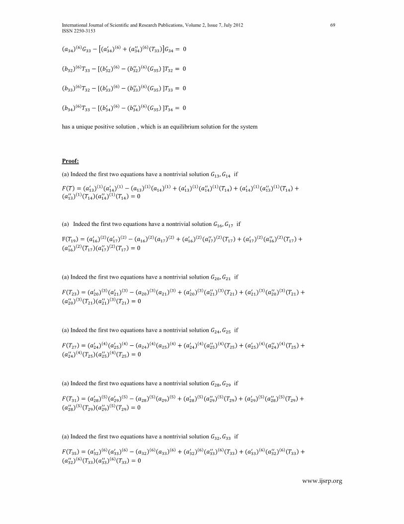
International Journal of Scientific and Research Publications, Volume 2, Issue 7, July 2012 69
ISSN 2250-3153
www.ijsrp.org
����������� − �����0 ���� + ����00 ������������� = 0
����������� − [����0 ���� − ����00 ��������� ]��� = 0
����������� − [����0 ���� − ����00 ��������� ]��� = 0
����������� − [����0 ���� − ����00 ��������� ]��� = 0
has a unique positive solution , which is an equilibrium solution for the system
Proof:
(a) Indeed the first two equations have a nontrivial solution ���, ��� if Ó��� = ����0 ��������0 ���� − ���������������� + ����0 ��������00 ��������� + ����0 ��������00 ��������� +����00 �������������00 ��������� = 0
(a) Indeed the first two equations have a nontrivial solution ���, �� if F��� � = ����0 �������0 ���� − ��������������� + ����0 �������00 �������� + ���0 ��������00 �������� +����00 �����������00 �������� = 0
(a) Indeed the first two equations have a nontrivial solution ���, ��� if Ó����� = ����0 ��������0 ���� − ���������������� + ����0 ��������00 ��������� + ����0 ��������00 ��������� +����00 �������������00 ��������� = 0
(a) Indeed the first two equations have a nontrivial solution ���, ��� if Ó���� = ����0 ��������0 ���� − ���������������� + ����0 ��������00 ��������� + ����0 ��������00 ��������� +����00 �������������00 ��������� = 0
(a) Indeed the first two equations have a nontrivial solution ��, �� if Ó����� = ���0 ������� 0 ���� − ���������� ���� + ���0 ������� 00 ������� � + ��� 0 �������00 ������� � +���00 ������� ���� 00 ������� � = 0
(a) Indeed the first two equations have a nontrivial solution ���, ��� if Ó����� = ����0 ��������0 ���� − ���������������� + ����0 ��������00 ��������� + ����0 ��������00 ��������� +����00 �������������00 ��������� = 0

International Journal of Scientific and Research Publications, Volume 2, Issue 7, July 2012 70
ISSN 2250-3153
www.ijsrp.org
Definition and uniqueness of T��∗ :-
After hypothesis =�0� < 0, =�∞� > 0 and the functions ��M00��������� being increasing, it follows
that there exists a unique ���∗ for which =����∗ � = 0. With this value , we obtain from the three first
equations
��� = �g�������� ��g�� ����|�g�� �����$� ∗ �� , ��� = �g�!������ ��g�! ����|�g�! �����$� ∗ ��
Definition and uniqueness of T�∗ :-
After hypothesis =�0� < 0, =�∞� > 0 and the functions ��M00�������� being increasing, it follows
that there exists a unique T�∗ for which =�T�∗ � = 0. With this value , we obtain from the three first
equations
��� = �g�%��(�^�&��g�% ��(�|�g�% ��(��ª�&∗ �� , �� = �g�'��(�^�&��g�' ��(�|�g�' ��(��ª�&∗ ��
Definition and uniqueness of T��∗ :-
After hypothesis =�0� < 0, =�∞� > 0 and the functions ��M00��������� being increasing, it follows
that there exists a unique ���∗ for which =����∗ � = 0. With this value , we obtain from the three first
equations
��� = �g()�����(���g() ����|�g() �����$(�∗ �� , ��� = �g((�����(���g(( ����|�g(( �����$(�∗ ��
Definition and uniqueness of T��∗ :-
After hypothesis =�0� < 0, =�∞� > 0 and the functions ��M00��������� being increasing, it follows
that there exists a unique ���∗ for which =����∗ � = 0. With this value , we obtain from the three first
equations
��� = �g( �� ��(!��g( �� �|�g( �� ��$(!∗ �� , ��� = �g(%�� ��(!��g(% �� �|�g(% �� ��$(!∗ ��
Definition and uniqueness of T� ∗ :-
After hypothesis =�0� < 0, =�∞� > 0 and the functions ��M00������� � being increasing, it follows
that there exists a unique �� ∗ for which =��� ∗ � = 0. With this value , we obtain from the three first
equations
�� = �g('��!��(*��g(' ��!�|�g(' ��!��$(*∗ �� , ��� = �g�)��!��(*��g�) ��!�|�g�) ��!��$(*∗ ��
Definition and uniqueness of T��∗ :-
After hypothesis =�0� < 0, =�∞� > 0 and the functions ��M00��������� being increasing, it follows
that there exists a unique ���∗ for which =����∗ � = 0. With this value , we obtain from the three first
equations
��� = �g�(��%������g�( ��%�|�g�( ��%��$��∗ �� , ��� = �g� ��%������g� ��%�|�g� ��%��$��∗ ��
(e) By the same argument, the equations (GLOBAL) admit solutions ���, ��� if
Ö��� = ����0 ��������0 ���� − ���������������� −

International Journal of Scientific and Research Publications, Volume 2, Issue 7, July 2012 71
ISSN 2250-3153
www.ijsrp.org
�����0 ��������00 ������� + ����0 ��������00 ��������+����00 �����������00 ������� = 0
Where in �����, ���, ����, ���, ��� must be replaced by their values from 96. It is easy to see that φ
is a decreasing function in ��� taking into account the hypothesis Ö�0� > 0 , Ö�∞� < 0 it follows
that there exists a unique ���∗ such that Ö��∗� = 0
(f) By the same argument, the equations (GLOBAL) admit solutions ���, �� if
φ��� � = ����0 �������0 ���� − ��������������� −
�����0 �������00 ������� � + ���0 ��������00 ������� ��+����00 ������� ����00 ������� � = 0
Where in ��� �����, ��, ���, ���, �� must be replaced by their values It is easy to see that φ is a
decreasing function in �� taking into account the hypothesis φ�0� > 0 , Ö�∞� < 0 it follows that
there exists a unique G��∗ such that φ���� �∗� = 0
(g) By the same argument, the equations(GLOBAL) admit solutions ���, ��� if
Ö����� = ����0 ��������0 ���� − ���������������� −
�����0 ��������00 ��������� + ����0 ��������00 ����������+����00 �������������00 ��������� = 0
Where in �������, ���, ����, ���, ��� must be replaced by their values . It is easy to see that φ is a
decreasing function in ��� taking into account the hypothesis Ö�0� > 0 , Ö�∞� < 0 it follows that
there exists a unique ���∗ such that Ö������∗� = 0
(h) By the same argument, the equations (GLOBAL) admit solutions ���, ��� if
Ö���� = ����0 ��������0 ���� − ���������������� −
�����0 ��������00 �������� + ����0 ��������00 ���������+����00 ������������00 �������� = 0
Where in ��������, ���, ����, ���, ��� must be replaced by their values from 96. It is easy to see that φ is a decreasing function in ��� taking into account the hypothesis Ö�0� > 0 , Ö�∞� < 0 it follows
that there exists a unique ���∗ such that Ö�����∗� = 0
(i) By the same argument, the equations (GLOBAL) admit solutions ��, �� if
Ö����� = ���0 ������� 0 ���� − ���������� ���� −
����0 ������� 00 ��������� + ��� 0 �������00 ����������+���00 ������������ 00 ��������� = 0
Where in ��������, �� , ����, ��, ��� must be replaced by their values It is easy to see that φ is a
decreasing function in �� taking into account the hypothesis Ö�0� > 0 , Ö�∞� < 0 it follows that
there exists a unique �� ∗ such that Ö������∗� = 0
(j) By the same argument, the equations(GLOBAL) admit solutions ���, ��� if
Ö����� = ����0 ��������0 ���� − ���������������� −
�����0 ��������00 ��������� + ����0 ��������00 ����������+����00 �������������00 ��������� = 0
Where in ���������, ���, ����, ���, ��� must be replaced by their values It is easy to see that φ is a
decreasing function in ��� taking into account the hypothesis Ö�0� > 0 , Ö�∞� < 0 it follows that

International Journal of Scientific and Research Publications, Volume 2, Issue 7, July 2012 72
ISSN 2250-3153
www.ijsrp.org
there exists a unique ���∗ such that Ö��∗� = 0
Finally we obtain the unique solution
���∗ given by Ö��∗� = 0 , ���∗ given by =����∗ � = 0 and
���∗ = �g�������� ∗��g�� ����|�g�� �����$� ∗ �� , ���∗ = �g�!������ ∗��g�! ����|�g�! �����$� ∗ �� ���∗ = �i������$� ∗��i�� ����a�i�� ������∗�� , ���∗ = �i�!����$� ∗��i�! ����a�i�! ������∗�� Obviously, these values represent an equilibrium solution
Finally we obtain the unique solution
G�∗ given by φ���� �∗� = 0 , T�∗ given by =�T�∗ � = 0 and
G��∗ = �Ú�%��(�^�&∗��Ú�% ��(�|�Ú�% ��(��ª�&∗ �� , G�∗ = �Ú�'��(�^�&∗��Ú�' ��(�|�Ú�' ��(��ª�&∗ ��
T��∗ = �Û�%��(�ª�&∗��Û�% ��(�a�Û�% ��(�����*�∗�� , T�∗ = �Û�'��(�ª�&∗��Û�' ��(�a�Û�' ��(�����*�∗��
Obviously, these values represent an equilibrium solution
Finally we obtain the unique solution
by Ö������∗� = 0 , ���∗ given by =����∗ � = 0 and
���∗ = �g()�����(�∗��g() ����|�g() �����$(�∗ �� , ���∗ = �g((�����(�∗��g(( ����|�g(( �����$(�∗ �� ���∗ = �i()����$(�∗��i() ����a�i() ������(�∗�� , ���∗ = �i((����$(�∗��i(( ����a�i(( ������(�∗�� Obviously, these values represent an equilibrium solution
Finally we obtain the unique solution
���∗ given by Ö���� = 0 , ���∗ given by =����∗ � = 0 and
���∗ = �g( �� ��(!∗��g( �� �|�g( �� ��$(!∗ �� , ���∗ = �g(%�� ��(!∗��g(% �� �|�g(% �� ��$(!∗ ��
���∗ = �i( �� �$(!∗��i( �� �a�i( �� ����(&�∗�� , ���∗ = �i(%�� �$(!∗��i(% �� �a�i(% �� ����(&�∗�� Obviously, these values represent an equilibrium solution
Finally we obtain the unique solution
�� ∗ given by Ö������∗� = 0 , �� ∗ given by =��� ∗ � = 0 and
��∗ = �g('��!��(*∗��g(' ��!�|�g(' ��!��$(*∗ �� , ���∗ = �g�)��!��(*∗��g�) ��!�|�g�) ��!��$(*∗ ��
��∗ = �i('��!�$(*∗��i(' ��!�a�i(' ��!�������∗�� , ���∗ = �i�)��!�$(*∗��i�) ��!�a�i�) ��!�������∗��

International Journal of Scientific and Research Publications, Volume 2, Issue 7, July 2012 73
ISSN 2250-3153
www.ijsrp.org
Obviously, these values represent an equilibrium solution
Finally we obtain the unique solution
���∗ given by Ö������∗� = 0 , ���∗ given by =����∗ � = 0 and
���∗ = �g�(��%����∗��g�( ��%�|�g�( ��%��$��∗ �� , ���∗ = �g� ��%����∗��g� ��%�|�g� ��%��$��∗ ��
���∗ = �i�(��%�$��∗��i�( ��%�a�i�( ��%�����!�∗�� , ���∗ = �i� ��%�$��∗��i� ��%�a�i� ��%�����!�∗�� Obviously, these values represent an equilibrium solution
ASYMPTOTIC STABILITY ANALYSIS
Theorem 4: If the conditions of the previous theorem are satisfied and if the functions ��M00���� �C8 ��M00���� Belong to Ï���� ℝ|� then the above equilibrium point is asymptotically stable.
Proof: Denote
Definition of ÜM, ÝM :- �M = �M∗ + ÜM , �M = �M∗ + ÝM Þ�g� ����Þ$� ����∗ � = �ß������ , Þ�ih ����Þ�� � �∗ � = ?M�
Then taking into account equations (GLOBAL) and neglecting the terms of power 2, we obtain
�Ü���� = −�����0 ���� + �S�������Ü�� + ��������Ü�� − �ß���������∗ Ý��
�Ü� �� = −�����0 ���� + �S�������Ü�� + ��������Ü�� − �ß���������∗ Ý��
�Ü�!�� = −�����0 ���� + �S�������Ü�� + ��������Ü�� − �ß���������∗ Ý��
�Ý���� = −�����0 ���� − �<�������Ý�� + ��������Ý�� + à �?����������∗ Ü�����á��
�Ý� �� = −�����0 ���� − �<�������Ý�� + ��������Ý�� + à �?����������∗ Ü�����á��
�Ý�!�� = −�����0 ���� − �<�������Ý�� + ��������Ý�� + à �?����������∗ Ü�����á��
If the conditions of the previous theorem are satisfied and if the functions �aM00���� and �bM00���� Belong to C���� ℝ|� then the above equilibrium point is asymptotically stable
Denote
Definition of ÜM, ÝM :-
GM = GM∗ + ÜM , TM = TM∗ + ÝM
â�g�& ��(�âª�& �T�∗ � = �ß����� , â�ih ��(�â^� � ��� �∗ � = ?M�
«Ü�%«¨ = −�����0 ���� + �S�������Ü�� + ��������Ü� − �ß������G��∗ Ý�

International Journal of Scientific and Research Publications, Volume 2, Issue 7, July 2012 74
ISSN 2250-3153
www.ijsrp.org
«Ü�&«¨ = −����0 ���� + �S������Ü� + �������Ü�� − �ß�����G�∗ Ý�
«Ü�'«¨ = −����0 ���� + �S������Ü� + �������Ü� − �ß�����G�∗ Ý�
«Ý�%«¨ = −�����0 ���� − �<�������Ý�� + ��������Ý� + à �?�������T��∗ Ü����á��
«Ý�&«¨ = −����0 ���� − �<������Ý� + �������Ý�� + à �?������T�∗ Ü����á��
«Ý�'«¨ = −����0 ���� − �<������Ý� + �������Ý� + à �?������T�∗ Ü����á��
If the conditions of the previous theorem are satisfied and if the functions ��M00���� �C8 ��M00���� Belong to Ï���� ℝ|� then the above equilibrium point is asymptotically stable
Denote
Definition of ÜM, ÝM :- �M = �M∗ + ÜM , �M = �M∗ + ÝM Þ�g(� ����Þ$(� ����∗ � = �ß������ , Þ�ih ����Þ�� � �����∗ � = ?M�
�Ü()�� = −�����0 ���� + �S�������Ü�� + ��������Ü�� − �ß���������∗ Ý��
�Ü(��� = −�����0 ���� + �S�������Ü�� + ��������Ü�� − �ß���������∗ Ý��
�Ü((�� = −�����0 ���� + �S�������Ü�� + ��������Ü�� − �ß���������∗ Ý��
�Ý()�� = −�����0 ���� − �<�������Ý�� + ��������Ý�� + à �?����������∗ Ü�����á��
�Ý(��� = −�����0 ���� − �<�������Ý�� + ��������Ý�� + à �?����������∗ Ü�����á��
�Ý((�� = −�����0 ���� − �<�������Ý�� + ��������Ý�� + à �?����������∗ Ü�����á��
If the conditions of the previous theorem are satisfied and if the functions ��M00���� �C8 ��M00���� Belong to Ï���� ℝ|� then the above equilibrium point is asymptotically stable
Denote
Definition of ÜM, ÝM :- �M = �M∗ + ÜM , �M = �M∗ + ÝM
Þ�g(! �� �Þ$(! ����∗ � = �ß������ , Þ�ih �� �Þ�� �����∗ � = ?M�
�Ü( �� = −�����0 ���� + �S�������Ü�� + ��������Ü�� − �ß���������∗ Ý��

International Journal of Scientific and Research Publications, Volume 2, Issue 7, July 2012 75
ISSN 2250-3153
www.ijsrp.org
�Ü(!�� = −�����0 ���� + �S�������Ü�� + ��������Ü�� − �ß���������∗ Ý��
�Ü(%�� = −�����0 ���� + �S�������Ü�� + ��������Ü�� − �ß���������∗ Ý��
�Ý( �� = −�����0 ���� − �<�������Ý�� + ��������Ý�� + à �?����������∗ Ü�����á��
�Ý(!�� = −�����0 ���� − �<�������Ý�� + ��������Ý�� + à �?����������∗ Ü�����á��
�Ý(%�� = −�����0 ���� − �<�������Ý�� + ��������Ý�� + à �?����������∗ Ü�����á��
If the conditions of the previous theorem are satisfied and if the functions ��M00���� �C8 ��M00���� Belong to Ï���� ℝ|� then the above equilibrium point is asymptotically STABLE
Denote
Definition of ÜM, ÝM :- �M = �M∗ + ÜM , �M = �M∗ + ÝM Þ�g(* ��!�Þ$(* ��� ∗ � = �ß� ���� , Þ�ih ��!�Þ�� � �����∗ � = ?M�
�Ü('�� = −����0 ���� + �S������Ü� + �������Ü� − �ß�������∗ Ý�
�Ü(*�� = −���� 0 ���� + �S� �����Ü� + ��� ����Ü� − �ß� ������ ∗ Ý�
�Ü�)�� = −�����0 ���� + �S�������Ü�� + ��������Ü� − �ß���������∗ Ý�
�Ý('�� = −����0 ���� − �<������Ý� + �������Ý� + à �?��������∗ Ü�����á�
�Ý(*�� = −���� 0 ���� − �<� �����Ý� + ��� ����Ý� + à �?�� ������ ∗ Ü�����á�
�Ý�)�� = −�����0 ���� − �<�������Ý�� + ��������Ý� + à �?����������∗ Ü�����á�
If the conditions of the previous theorem are satisfied and if the functions ��M00���� �C8 ��M00���� Belong to Ï���� ℝ|� then the above equilibrium point is asymptotically stable
Denote
Definition of ÜM, ÝM :- �M = �M∗ + ÜM , �M = �M∗ + ÝM
Þ�g�� ��%�Þ$�� ����∗ � = �ß������ , Þ�ih ��%�Þ�� � �����∗ � = ?M�
�Ü�(�� = −�����0 ���� + �S�������Ü�� + ��������Ü�� − �ß���������∗ Ý��

International Journal of Scientific and Research Publications, Volume 2, Issue 7, July 2012 76
ISSN 2250-3153
www.ijsrp.org
�Ü���� = −�����0 ���� + �S�������Ü�� + ��������Ü�� − �ß���������∗ Ý��
�Ü� �� = −�����0 ���� + �S�������Ü�� + ��������Ü�� − �ß���������∗ Ý��
�Ý�(�� = −�����0 ���� − �<�������Ý�� + ��������Ý�� + à �?����������∗ Ü�����á��
�Ý���� = −�����0 ���� − �<�������Ý�� + ��������Ý�� + à �?����������∗ Ü�����á��
�Ý� �� = −�����0 ���� − �<�������Ý�� + ��������Ý�� + à �?����������∗ Ü�����á��
The characteristic equation of this system is
��ã���� + ����0 ���� − �<�������{��ã���� + ����0 ���� + �S�������
"���ã���� + ����0 ���� + �S��������ß���������∗ + ���������ß���������∗ �#
���ã���� + ����0 ���� − �<�������?����,�������∗ +��������?����,�������∗ �
+ ���ã���� + ����0 ���� + �S��������ß���������∗ + ���������ß���������∗ �
���ã���� + ����0 ���� − �<�������?����,�������∗ + ��������?����,�������∗ �
�������� + � ����0 ���� + ����0 ���� + �S������ + �S������� �����
���ã������ + � ����0 ���� + ����0 ���� − �<������ + �<������� �ã�����
+ �������� + � ����0 ���� + ����0 ���� + �S������ + �S������� ����� ����������
+��ã���� + ����0 ���� + �S������� ����������ß���������∗ + �����������������ß���������∗ � ���ã���� + ����0 ���� − �<�������?����,�������∗ +��������?����,�������∗ �} = 0
+
��ã���� + ���0 ���� − �<������{��ã���� + ���0 ���� + �S������
"���ã���� + ����0 ���� + �S��������ß�����G�∗ + ��������ß������G��∗ �#
���ã���� + ����0 ���� − �<�������?���,���T�∗ +�������?����,���T�∗ �
+ ���ã���� + ���0 ���� + �S�������ß������G��∗ + ���������ß�����G�∗ �
���ã���� + ����0 ���� − �<�������?���,����T�∗ + �������?����,����T��∗ �
�������� + � ����0 ���� + ���0 ���� + �S������ + �S������ �����
���ã������ + � ����0 ���� + ���0 ���� − �<������ + �<������ �ã�����

International Journal of Scientific and Research Publications, Volume 2, Issue 7, July 2012 77
ISSN 2250-3153
www.ijsrp.org
+ �������� + � ����0 ���� + ���0 ���� + �S������ + �S������ ����� ������G�
+��ã���� + ����0 ���� + �S������� ���������ß�����G�∗ + ���������������ß������G��∗ � ���ã���� + ����0 ���� − �<�������?���,���T�∗ +�������?����,���T��∗ �} = 0
+
��ã���� + ����0 ���� − �<�������{��ã���� + ����0 ���� + �S�������
"���ã���� + ����0 ���� + �S��������ß���������∗ + ���������ß���������∗ �#
���ã���� + ����0 ���� − �<�������?����,�������∗ +��������?����,�������∗ �
+ ���ã���� + ����0 ���� + �S��������ß���������∗ + ���������ß���������∗ �
���ã���� + ����0 ���� − �<�������?����,�������∗ + ��������?����,�������∗ �
�������� + � ����0 ���� + ����0 ���� + �S������ + �S������� �����
���ã������ + � ����0 ���� + ����0 ���� − �<������ + �<������� �ã�����
+ �������� + � ����0 ���� + ����0 ���� + �S������ + �S������� ����� ����������
+��ã���� + ����0 ���� + �S������� ����������ß���������∗ + �����������������ß���������∗ � ���ã���� + ����0 ���� − �<�������?����,�������∗ +��������?����,�������∗ �} = 0
+
��ã���� + ����0 ���� − �<�������{��ã���� + ����0 ���� + �S�������
"���ã���� + ����0 ���� + �S��������ß���������∗ + ���������ß���������∗ �#
���ã���� + ����0 ���� − �<�������?����,�������∗ +��������?����,�������∗ �
+ ���ã���� + ����0 ���� + �S��������ß���������∗ + ���������ß���������∗ �
���ã���� + ����0 ���� − �<�������?����,�������∗ + ��������?����,�������∗ �
�������� + � ����0 ���� + ����0 ���� + �S������ + �S������� �����
���ã������ + � ����0 ���� + ����0 ���� − �<������ + �<������� �ã�����
+ �������� + � ����0 ���� + ����0 ���� + �S������ + �S������� ����� ����������
+��ã���� + ����0 ���� + �S������� ����������ß���������∗ + �����������������ß���������∗ �

International Journal of Scientific and Research Publications, Volume 2, Issue 7, July 2012 78
ISSN 2250-3153
www.ijsrp.org
���ã���� + ����0 ���� − �<�������?����,�������∗ +��������?����,�������∗ �} = 0
+
��ã���� + ����0 ���� − �<�������{��ã���� + ����0 ���� + �S�������
"���ã���� + ���0 ���� + �S�������ß� ������ ∗ + ��� �����ß�������∗ �# ���ã���� + ���0 ���� − �<������?�� �,�� ��� ∗ +��� ����?���,�� ��� ∗ �
+ ���ã���� + ��� 0 ���� + �S� ������ß�������∗ + ��������ß� ������ ∗ �
���ã���� + ���0 ���� − �<������?�� �,����� ∗ + ��� ����?���,�����∗ �
�������� + � ���0 ���� + ��� 0 ���� + �S����� + �S� ����� �����
���ã������ + � ���0 ���� + ��� 0 ���� − �<����� + �<� ����� �ã�����
+ �������� + � ���0 ���� + ��� 0 ���� + �S����� + �S� ����� ����� ����������
+��ã���� + ���0 ���� + �S������ ����������ß� ������ ∗ + ��� �������������ß�������∗ � ���ã���� + ���0 ���� − �<������?�� �,������ ∗ +��� ����?���,������∗ �} = 0
+
��ã���� + ����0 ���� − �<�������{��ã���� + ����0 ���� + �S�������
"���ã���� + ����0 ���� + �S��������ß���������∗ + ���������ß���������∗ �#
���ã���� + ����0 ���� − �<�������?����,�������∗ +��������?����,�������∗ �
+ ���ã���� + ����0 ���� + �S��������ß���������∗ + ���������ß���������∗ �
���ã���� + ����0 ���� − �<�������?����,�������∗ + ��������?����,�������∗ �
�������� + � ����0 ���� + ����0 ���� + �S������ + �S������� �����
���ã������ + � ����0 ���� + ����0 ���� − �<������ + �<������� �ã�����
+ �������� + � ����0 ���� + ����0 ���� + �S������ + �S������� ����� ����������
+��ã���� + ����0 ���� + �S������� ����������ß���������∗ + �����������������ß���������∗ � ���ã���� + ����0 ���� − �<�������?����,�������∗ +��������?����,�������∗ �} = 0
And as one sees, all the coefficients are positive. It follows that all the roots have negative real part,
and this proves the theorem.

International Journal of Scientific and Research Publications, Volume 2, Issue 7, July 2012 79
ISSN 2250-3153
www.ijsrp.org
Acknowledgments:
The introduction is a collection of information from various articles, Books, News Paper
reports, Home Pages Of authors, Artists images, Journal Reviews, Article abstracts, NASA
PHOTOGRAPHS, Stanford Encyclopedia, IV League University Library Search,Text Books,
and Others Books available online, . the internet including Wikipedia. We acknowledge all
authors who have contributed to the same. In the eventuality of the fact that there has been any
act of omission on the part of the authors, We regret with great deal of compunction, contrition,
and remorse. As Newton said, it is only because erudite and eminent people allowed one to
piggy ride on their backs; probably an attempt has been made to look slightly further. Once
again, it is stated that the references are only illustrative and not comprehensive. Without these
sources, the preparation of the paper would have been a bête noir, a la non consummatus. We
pay homage to all sources.
REFERENCES
Dr K N Prasanna Kumar, Prof B S Kiranagi, Prof C S Bagewadi - MEASUREMENT DISTURBS
EXPLANATION OF QUANTUM MECHANICAL STATES-A HIDDEN VARIABLE THEORY -
published at: "International Journal of Scientific and Research Publications, Volume 2, Issue 5, May
2012 Edition".
DR K N PRASANNA KUMAR, PROF B S KIRANAGI and PROF C S BAGEWADI -CLASSIC 2
FLAVOUR COLOR SUPERCONDUCTIVITY AND ORDINARY NUCLEAR MATTER-A NEW
PARADIGM STATEMENT - published at: "International Journal of Scientific and Research
Publications, Volume 2, Issue 5, May 2012 Edition". A HAIMOVICI: “On the growth of a two species ecological system divided on age groups”. Tensor,
Vol 37 (1982),Commemoration volume dedicated to Professor Akitsugu Kawaguchi on his 80th
birthday
FRTJOF CAPRA: “The web of life” Flamingo, Harper Collins See "Dissipative structures” pages
172-188
HEYLIGHEN F. (2001): "The Science of Self-organization and Adaptivity", in L. D. Kiel, (ed) .
Knowledge Management, Organizational Intelligence and Learning, and Complexity, in: The
Encyclopedia of Life Support Systems ((EOLSS), (Eolss Publishers, Oxford) [http://www.eolss.net
MATSUI, T, H. Masunaga, S. M. Kreidenweis, R. A. Pielke Sr., W.-K. Tao, M. Chin, and Y. J
Kaufman (2006), “Satellite-based assessment of marine low cloud variability associated with
aerosol, atmospheric stability, and the diurnal cycle”, J. Geophys. Res., 111, D17204,
doi:10.1029/2005JD006097
STEVENS, B, G. Feingold, W.R. Cotton and R.L. Walko, “Elements of the microphysical structure
of numerically simulated nonprecipitating stratocumulus” J. Atmos. Sci., 53, 980-1006
FEINGOLD, G, Koren, I; Wang, HL; Xue, HW; Brewer, WA (2010), “Precipitation-generated
oscillations in open cellular cloud fields” Nature, 466 (7308) 849-852, doi: 10.1038/nature09314,
Published 12-Aug 2010
R WOOD “The rate of loss of cloud droplets by coalescence in warm clouds” J.Geophys. Res., 111,
doi: 10.1029/2006JD007553, 2006
H. RUND, “The Differential Geometry of Finsler Spaces”, Grund. Math. Wiss. Springer-Verlag,
Berlin, 1959

International Journal of Scientific and Research Publications, Volume 2, Issue 7, July 2012 80
ISSN 2250-3153
www.ijsrp.org
A. Dold, “Lectures on Algebraic Topology”, 1972, Springer-Verlag
S LEVIN “Some Mathematical questions in Biology vii ,Lectures on Mathematics in life sciences,
vol 8” The American Mathematical society, Providence , Rhode island 1976
[13] E. Knill, R. Laflamme, and G. J. Milburn, “A scheme for efficient quantum computation with
linear optics’’, Nature 409, 46 (2001).
[14] R. Raussendorf and H. J. Briegel, “A one-way quantum computer’’, Phys. Rev. Lett. 86, 5188
(2001).
[15] P. Walther, K. J. Resch, T. Rudolph, E. Schenck, H. Weinfurter, V. Vedral, M. Aspelmeyer, and
A. Zeilinger, “Experimental one-way quantum computing”, Nature 434, 169 (2005).
[16] R. Prevedel, P. Walther, F. Tiefenbacher, P. Böhi, R. Kaltenbaek, T. Jennewein, and A.
Zeilinger, "High-speed linear optics quantum computing using active feed-forward", Nature 445, 65
(2007)
[17] D. N. Biggerstaff, R. Kaltenbaek, D. R. Hamel, G. Weihs, T. Rudolph, and K. J. Resch, "Cluster-
State Quantum Computing Enhanced by High-Fidelity Generalized Measurements.", Phys. Rev. Lett.
103, 240504 (2009)
[18] M. Cramer, M. B. Plenio, "Reconstructing quantum states efficiently", e-print arXiv: 1002.3780
[19] S. T. Flammia, D. Gross, S. D. Bartlett, and R. Somma, "Heralded Polynomial-Time Quantum
State Tomography", e-print arXiv: 1002.3839
[20] A. Peruzzo, A. Laing, A. Politi, T. Rudolph, and J. L. O'Brien, "Multimode quantum interference
of photons in multiport integrated devices", e-print arXiv: 1007.1372
21. ^ Technical Report MIT/LCS/TM-151 (1980) and an adapted and condensed version: Toffoli,
Tommaso (1980). "Reversible computing". In J. W. de Bakker and J. van Leeuwen. Automata,
Languages and Programming, Seventh Colloquium. Noordwijkerhout, Netherlands: Springer Verlag.
pp. 632-644. ISBN 3-540-10003-2.
22. ^ Barenco, Adriano; Bennett, Charles H.; Richard, Cleve; DiVincenzo, David P.; Margolus,
Norman; Shor, Peter; Sleator, Tycho; Smolin, John A. et al. (Nov 1995). "Elementary gates for
quantum computation". Phys. Rev. A (American Physical Society) 52 (5): 3457–3467. ArXiv: quant-
ph/9503016. DOI:10.1103/PhysRevA.52.3457. PMID 9912645.
23. ^ Fredkin, Edward; Toffoli, Tommaso (April 1982). "Conservative logic". International Journal
of Theoretical Physics (Springer Netherlands) 21 (3): 219–
253.DOI:10.1007/BF01857727. ISSN 0020-7748.
24. ^ Monz, T.; Kim, K.; Hänsel, W.; Riebe, M.; Villar, A. S.; Schindler, P.; Chwalla, M.; Hennrich,
M. et al. (Jan 2009). "Realization of the Quantum Toffoli Gate with Trapped Ions". R. (American
Physical Society) 102 (4): 040501. ArXiv:
0804.0082. Bibcode 2009PhRvL.102d0501M. DOI:10.1103/PhysRevLett.102.040501.
International Journal of Scientific and Research Publications, Volume 2, Issue 7, July 2012 81
ISSN 2250-3153
www.ijsrp.org
First Author: 1Mr. K. N.Prasanna Kumar has three doctorates one each in Mathematics, Economics,
Political Science. Thesis was based on Mathematical Modeling. He was recently awarded D.litt., for his work on
‘Mathematical Models in Political Science’--- Department of studies in Mathematics, Kuvempu University,
Shimoga, Karnataka, India Corresponding Author:[email protected]
Second Author: 2Prof. B.S Kiranagi is the Former Chairman of the Department of Studies in Mathematics,
Manasa Gangotri and present Professor Emeritus of UGC in the Department. Professor Kiranagi has guided
over 25 students and he has received many encomiums and laurels for his contribution to Co homology Groups
and Mathematical Sciences. Known for his prolific writing, and one of the senior most Professors of the
country, he has over 150 publications to his credit. A prolific writer and a prodigious thinker, he has to his credit
several books on Lie Groups, Co Homology Groups, and other mathematical application topics, and excellent
publication history.-- UGC Emeritus Professor (Department of studies in Mathematics), Manasagangotri,
University of Mysore, Karnataka, India
Third Author: 3Prof. C.S. Bagewadi is the present Chairman of Department of Mathematics and Department
of Studies in Computer Science and has guided over 25 students. He has published articles in both national and
international journals. Professor Bagewadi specializes in Differential Geometry and its wide-ranging
ramifications. He has to his credit more than 159 research papers. Several Books on Differential Geometry,
Differential Equations are coauthored by him--- Chairman, Department of studies in Mathematics and Computer
science, Jnanasahyadri Kuvempu university, Shankarghatta, Shimoga district, Karnataka, India