of potential impacts on water levels and land subsidence ... · appendix h predictions of potential...

APPENDIX H

Predictions of Potential Impacts on

Water Levels and Land Subsidence in

Brazoria County Report

November 2013

PredictionsofPotentialImpactsonWaterLevelsandLandSubsidencecausedbyWellFieldsnearBrazosportWater

AuthorityPlantinBrazoriaCounty

Final Report

December 2013

i

Contents

1.0 Background ............................................................................................................................ 1

2.0 Simulation of Historical Groundwater Level and Land Subsidence in the HAGM ................ 3

3.0 Potential Impacts of Future Groundwater Pumping on Water Levels and Land Subsidence Predicted by the HAGM ..................................................................................... 4

4.0 Simulation of Historical and Future Groundwater Levels and Land Subsidence using the LCRB Model ........................................................................................................... 5

5.0 Comparison Between Clay Thicknesses and Aquifer Parameters in the HAGM that Affect Predicted Subsidence .......................................................................................... 7

6.0 Summary ............................................................................................................................... 8

7.0 References ............................................................................................................................. 9

ListofTables

Table 1. Calculated RMS for the HAGM and LCRB model from 1920 through the end of 2006. ................................................................................................. 34

ii

ListofFigures

Figure 1. Location of the proposed well field in Brazoria County, Texas. ........................ 10

Figure 2. Model extents of the HAGM model and the LCRB model and the proposed well field. ........................................................................................... 10

Figure 3. Pumping in Brazoria County in the HAGM. ....................................................... 11

Figure 4. Historical water level and land subsidence in Chicot Aquifer simulated by the HAGM at the proposed well field. ......................................... 11

Figure 5. Drawdown and subsidence simulated by the HAGM for 2005. ........................ 12

Figure 6. TWDB wells used for RMSE calculation (orange circles) around the well field. ............................................................................................................ 13

Figure 7. Locations of the additional water production wells in the HAGM model grid for pumping scenario 1 and pumping scenario 2: wells 1 and 2 are freshwater wells and wells 3 and 4 are brackish water wells. .................................................................................................................. 13

Figure 8. Locations of the additional water production wells in the HAGM model grid for pumping scenario 3: wells 1 and 2 are freshwater wells and wells 3 and 4 are brackish water wells. ............................................. 14

Figure 9. Simulated water level (in layer 1) and land subsidence in HAGM model baseline predictive model (baseline pumping scenario) at the well field. ............................................................................................................ 14

Figure 10. Simulated water level (in layer 1) and land subsidence in HAGM model predictive model with two fresh water wells (2,000 GPM) at the well field (pumping scenario 1). .................................................................. 15

Figure 11. Simulated water level (in layer 1) and land subsidence in HAGM model predictive model with two fresh water wells and two brackish water wells (4,000 GPM) at the well field (pumping scenario 2). ......................................................................................................... 15

Figure 12 Simulated water level (in layer 1) and land subsidence in HAGM model predictive model with two fresh water wells (across Brazos River) and two brackish water wells (4,000 GPM) at the well field (pumping scenario 3). ........................................................................................ 16

Figure 13. Drawdown (feet) from 2005 to 2050 in layer 1 of the baseline HAGM pumping scenario. .................................................................................. 16

Figure 14. Impacts of freshwater production from 2005 to 2020 (2,000 GPM) simulated by the HAGM for pumping scenario 1. ............................................. 17

Figure 15. Impacts of freshwater production from 2005 to 2035(2,000 GPM) simulated by the HAGM for pumping scenario 1. ............................................. 18

iii

Figure 16. Impacts of freshwater production from 2005 to 2050 (2,000 GPM) simulated by the HAGM for pumping scenario 1. ............................................. 19

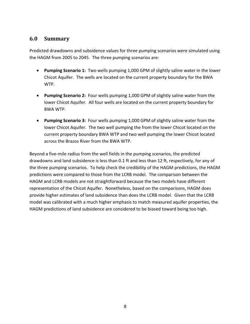
Figure 17. Impacts of fresh and brackish water production from 2005 to 2020 (4,000 GPM) simulated by the HAGM for pumping scenario 2. ........................ 20



Figure 20. Impacts of freshwater (wells located across Brazos River) and brackish water production from 2005 to 2020 (4,000 GPM) simulated by the HAGM for pumping scenario 3. ............................................. 23



Figure 23. Simulated water level at the well field in the HAGM and the LCRB model before 2005. ........................................................................................... 26

Figure 24. Simulated land subsidence at the well field in the HAGM and the LCRB model before 2005. .................................................................................. 26

Figure 25. Simulated water level at the well field in the baseline predictive runs based on HAGM and the LCRB model after 2005. .................................... 27

Figure 26. Simulated land subsidence at the well field in the baseline predictive runs based on HAGM and the LCRB model for baseline pumping scenario after 2005. ............................................................................ 27

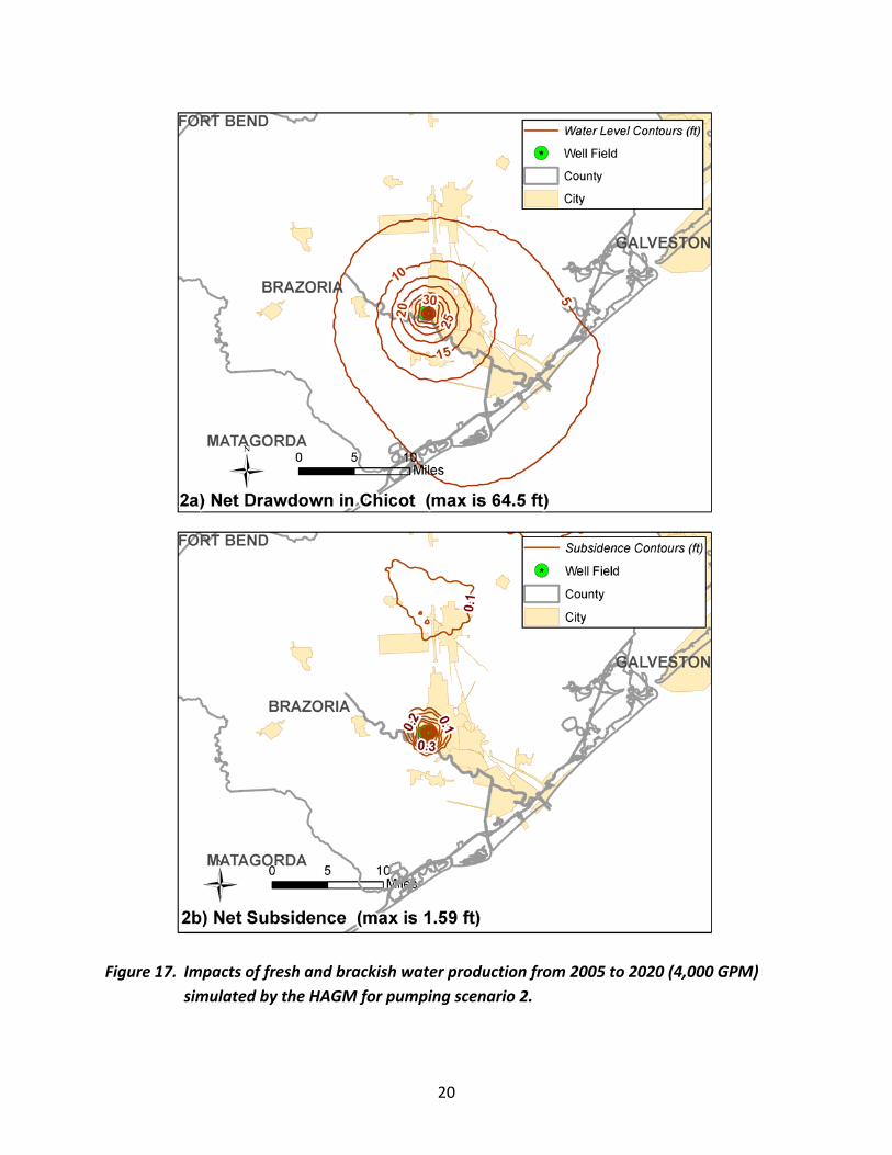
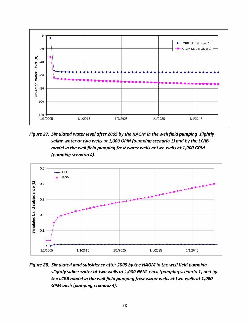
Figure 27. Simulated water level after 2005 by the HAGM in the well field pumping slightly saline water at two wells at 1,000 GPM (pumping scenario 1) and by the LCRB model in the well field pumping freshwater wells at two wells at 1,000 GPM (pumping scenario 4). ................. 28

Figure 28. Simulated land subsidence after 2005 by the HAGM in the well field pumping slightly saline water at two wells at 1,000 GPM each (pumping scenario 1) and by the LCRB model in the well field pumping freshwater wells at two wells at 1,000 GPM each (pumping scenario 4). ........................................................................................ 28

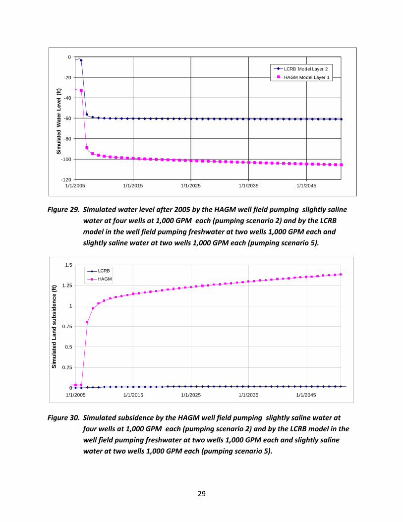
Figure 29. Simulated water level after 2005 by the HAGM well field pumping slightly saline water at four wells at 1,000 GPM each (pumping scenario 2) and by the LCRB model in the well field pumping

iv

freshwater at two wells 1,000 GPM each and slightly saline water at two wells 1,000 GPM each (pumping scenario 5). ............................................ 29

Figure 30. Simulated subsidence by the HAGM well field pumping slightly saline water at four wells at 1,000 GPM each (pumping scenario 2) and by the LCRB model in the well field pumping freshwater at two wells 1,000 GPM each and slightly saline water at two wells 1,000 GPM each (pumping scenario 5). ....................................................................... 29

Figure 31. Impacts on drawdown and subsidence simulated by the LCRB model (pumping scenario 4) caused by pumping fresh from 2005 to 2050 (2,000 GPM). ...................................................................................................... 30

Figure 32. Impacts on drawdown and subsidence simulated by the LCRB model (pumping scenario 5) caused by pumping fresh and slightly saline water production from 2005 to 2050 (4,000 GPM). ......................................... 31

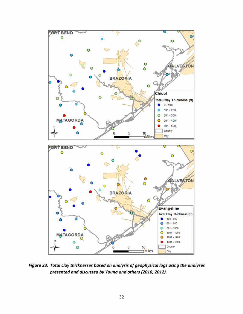
Figure 33. Total clay thicknesses based on analysis of geophysical logs using the analyses presented and discussed by Young and others (2010, 2012). ................................................................................................................. 32

Figure 34. Non‐elastic storage coefficients from the HAGM for the Chicot and Evangeline Aquifers. .......................................................................................... 33

v

ExecutiveSummary

This study was conducted to evaluate the impacts of future groundwater production near the

Brazos River Water Authority’s (BWA) water treatment plant (WTP) on groundwater drawdown

and land subsidence. The Houston Area Groundwater Model (HAGM) (Kasmarek, 2012) and the

Lower‐Colorado River Basin (LCRB) model (Young and others, 2009) were used to simulate the

impacts of pumping on water level and subsidence surrounding the proposed well fields. The

pumping scenarios simulated by the HAGM are:

Pumping Scenario 1: Two wells pumping 1,000 GPM of slightly saline water in the lower

Chicot Aquifer. The wells are located on the current property boundary for the BWA

WTP.

Pumping Scenario 2: Four wells pumping 1,000 GPM of slightly saline water from the

lower Chicot Aquifer. All four wells are located on the current property boundary for

BWA WTP.


lower Chicot Aquifer. The two well pumping the from the lower Chicot located on the

current property boundary BWA WTP and two well pumping the lower Chicot located

across the Brazos River from the BWA WTP.

Modeling results from the HAGM indicate that the impacts for all three pumping scenarios are

acceptable and will not adversely impact current well owners or land owners. For all three

scenarios, the predicted drawdown was less than 12 beyond a five‐mile radius from the wells

and the predicted land subsidence was less than 0.1 ft beyond a five‐mile radius from the wells.

The comparison of results between the HAGM and the LCRB model indicate that the HAGM

model may be over predicting both drawdown and land subsidence.

1

1.0 Background

The purpose of this study is to evaluate the potential for pumping in the vicinity of the

Brazosport Water Authority (BWA) Water Treatment Plant (WTP) to cause groundwater

drawdowns and land subsidence. Figure 1 shows the proposed well field in Brazoria County,

Texas. The well field scenarios pump water at rates between 2,000 gallons per minute (GPM

and 4,000 GPM from the Chicot Aquifer.

The Chicot aquifer is part of the Gulf Coast Aquifer System. Currently, Groundwater

Management Area 14 (GMA 14) is using the Houston Area Groundwater Model (HAGM)

(Kasmarek, 2012) for predicting regional changes to water levels caused by projected pumping

in the northern gulf coast aquifer system. To help check of the reasonableness of the HAGM

predictions, predictions from the Lower‐Colorado River Basin (LCRB) model (Young and others,

2009) are also performed for two of the pumping scenarios.

The HAGM is used to simulate three pumping scenarios from proposed wells near the

Brazosport Water Authority. The three simulations are:


Chicot Aquifer. The wells are located on the current property boundary for the

Brazosport Water Treatment Plant.



BWA WTP.


lower Chicot Aquifer ‐ two wells pumping the from the lower Chicot located on the

current property boundary for BWA WTP and two wells pumping the lower Chicot

located across the Brazos River from the BWAWTP.

The HAGM is a MODFLOW‐2000 (Harbaugh and others, 1996) groundwater flow model that

was developed by the United States Geologic Survey (Kasmarek, 2012) for the Northern Gulf

Coast Aquifer System. The HAGM model calibration period begins in 1900 and ends in 2009.

The model has four model layers that represent the Chicot Aquifer, Evangeline Aquifer, the

Burkeville Confining Layer, and the Jasper Aquifer. The grid cells are uniformly one square mile.

The HAGM was developed by revising the current GAM for GMA 14 (Kasmarek and Robinson,

2004).

2

The LCRB model is a MODFLOW‐SURFACT (HGL, 2005) groundwater flow model that was

developed by URS and INTERA for the Lower Colorado River Authority. The LCRB model

calibration period begins in 1900 and ends in 2006. The model has six model layers that

represent a shallow flow zone, the Beaumont Formation in the Chicot Aquifer, the Lissie

Formation in the Chicot Aquifer, the Willis Formation in the Chicot Aquifer, the Upper Goliad

Formation in the Evangeline Aquifer, and the Lower Goliad Formation in the Evangeline Aquifer.

The grid cells are non‐uniform with dimensions varying between 0.25 miles and one mile.

Figure 2 shows the model domain for the HAGM and the LCRB model. The two models overlap

coverage in Brazoria County. The development of the HAGM focused on the model calibration

on a five‐county area that included Brazoria County. The development of the LCRB Model

focused on the model calibration on Colorado, Wharton, and Matagorda Counties.

In a previous analyses of the Gulf Coast Aquifer in the vicinity of the Brazosport well field

(INTERA, 2012) the analysis of geophysical logs indicated that the upper Chicot and lower

Chicot contain fresh water and slightly saline water, respectively. INTERA (2012) defined fresh

water to have a Total Dissolved Solids (TDS) less than 1,000 parts per million (ppm) and defined

slightly saline water to have a TDS between 1,000 ppm and 3,000 ppm. Because the HAGM

model represents the Chicot Aquifer as one model layer and the HAGM assumes a well fully

penetrates the entire aquifer, the HAGM cannot differentiate between pumping the upper and

lower Chicot Aquifer. However, the LCRB model represents the Chicot as four different model

layers and therefore can be used to differentiate pumping between the upper and lower Chicot

Aquifer.

3

2.0 SimulationofHistoricalGroundwaterLevelandLandSubsidenceintheHAGM

Figure 3 shows the historical pumping in Brazoria County in the HAGM model. In Brazoria

County, pumping only occurs in the Chicot Aquifer and Evangeline Aquifer. Figure 4 presents

the historical water level and subsidence in Chicot Aquifer simulated by the HAGM model at the

proposed well field in the Chicot Aquifer from 1920 to 2006.

The HAGM was calibrated to measured water level and land subsidence from predevelop

conditions (~1900) to 2009. Figure 5 shows the drawdown and land subsidence the HAGM

simulated for 2005 relative to predevelopment conditions. Two potentially important

measures of a groundwater model’s ability to predict pumping impacts are an accurate

representation of the aquifer hydraulic properties and the ability to predict historical water

levels given that there is an accurate representation of historical pumping. To help evaluate the

HAGM, an assessment was made of how well the HAGM simulated water levels matched the

measured water levels within a 20 mile radius of the proposed well fields (see Figure 6). The

measured water levels were obtained from the Texas Water Development Board (TWDB)

groundwater database. The simulated water levels were extracted from the HAGM at the

locations of the TWDB wells that had more than four water level measurements (a total of 59

wells). Table 1 shows the calculated mean error and the root mean squared errors (RMSE) for

the 59 wells. The considerable spread in both set of numbers is attributed to simplifications in

the model structure, inaccuracies with representing the aquifer hydraulic properties, and

inaccuracies in the historical pumping. The average RMSE represents an estimate of the

average error in the simulating the water level. For the HAGM, the RMSE for the 59 wells is

about 34 feet. This amount of error has been considered acceptable by the TWDB (Wade and

others, 2013).

4

3.0 PotentialImpactsofFutureGroundwaterPumpingonWaterLevelsandLandSubsidencePredictedbytheHAGM

Four model runs were conducted using the HAGM to predict impacts of future groundwater

pumping on water levels and subsidence. The model runs are described below:

Baseline Pumping Scenario: Baseline predictive run (1900‐2050). The HAGM model was

temporally extended to 2050. The boundary conditions (including pumping locations

and rates) from the beginning of 2006 to the end of the simulation are identical to those

in year 2005. This run provides a baseline prediction assuming all the conditions

continue without variation.

Pumping Scenario 1: Baseline predictive run with two additional wells pumping slightly

saline water at 1,000 GPM each (2,000 GPM total), starting at the beginning of 2006 and

continuing until 2050. These two wells, represented by wells 1 and 2 in Figure 7, are

added into model layer 1 (Chicot).

Pumping Scenario 2. Baseline predictive run with the four wells (wells 1 through 4 in

Figure 7) pumping slightly saline water at 1,000 GPM each (4,000 GPM total), starting at

the beginning of 2006 and continuing until 2050. All of these four additional wells are

located in model layer 1 (Chicot).

Pumping Scenario 3. Baseline predictive run with two brackish freshwater wells across

the Brazos River (wells 1 and 2 in Figure 8) and two brackish water wells (wells 3 and 4 in

Figures 7 and 8) pumping at 1,000 GPM each (4,000 GPM total), starting at the

beginning of 2006 and continuing until the end of the model. All of these four additional

wells are located in model layer 1 (Chicot).

Figures 9 through 12 show the simulated water level and subsidence at the well field over time

(2006‐2050) for the baseline and three pumping scenarios. Contours of drawdown from 2005

to 2050 in model layer 1 are plotted in Figure 13 for the Baseline Pumping Scenario.

For Pumping Scenarios 1, 2, and 3, the difference of the simulation results (water level and

subsidence) and those from the Baseline Pumping Scenario shows the effect of production at

the well field. Figures 14 through 22 show the contours of net water level change and

subsidence caused by the well field pumping as simulated by the HAGM in years 2020, 2035

and 2050, for the three pumping scenarios.

5

4.0 SimulationofHistoricalandFutureGroundwaterLevelsandLandSubsidenceusingtheLCRBModel

Figures 23 and 24 show the simulated water level and subsidence for the historical period

(before 2005) in the LCRB model. For the convenience of comparison, the simulated values of

the HAGM model were plotted in the same figures as well. Table 1 shows how well the LCRB

matches the historical measurements of the measured water levels compared to the HAGM

model. The RMSE for the LCRB model and the HAGM are about 36 ft and 34 ft respectively.

Thus, the HAGM has a slightly better fit than the LCRB model. However, the LCRB was

calibrated to also match hydraulic conductivity values (Young and others, 2006) where the

calibration criteria listed by Kasmarek (2012, pg. 12) does not indicate that matching hydraulic

conductivity or any other measured aquifer hydraulic parameter was a part of the objective

function used to drive the calibration. The lack of objective constraints on the aquifer

parameters can lead to unrepresentative and even unrealistic hydraulic conductivity values.

During its calibration, the LCRB model was also constrained to develop aquifer parameters that

are developed from empirically based relationship between the measured physical properties

of the aquifer such as percent sand, depth of burial and depositional setting to constraint

hydraulic conductivity, and other aquifer parameters during model calibration. For these

reasons, the LCRB Model was used to simulate pumping scenarios so that results could be

compared to those produced by the HAGM. Descriptions of the three pumping scenarios

simulated by the LCRB model are as follows:

Baseline Pumping Scenario: (1900‐2050). From the beginning of 2006, the recharge

rate at each grid cell was set to the average recharge rate from 1900 through 2000; and

the pumping rate at each well was set as the average pumping in 2005. This run

provides a baseline prediction assuming all the conditions continue as an average

condition.

Pumping Scenario 4: Baseline predictive run with two additional wells pumping fresh

water at 1,000 GPM each (2,000 GPM total), starting at the beginning of 2006 and

continuing until 2050. These two wells, represented by wells 1 and 2 in Figure 7, are

added into model layer 2 (Beaumont).

Pumping Scenario 5: Baseline predictive run with two additional freshwater wells (wells

1 and 2 in Figure 7) and two brackish water wells (wells 3 and 4 in Figure 7) pumping at

1,000 GPM each (4,000 GPM total), starting at the beginning of 2006 and continuing

until 2050. The two freshwater wells are located in Model Layer 2 (Beaumont) and the

two brackish water wells are located in Model Layer 3 (Lissie).

6

Figures 25 through 30 show the simulated water level and subsidence at the well field over

time in the predictive period for the pumping scenarios. Figures 31 and 32 shows the net water

level and subsidence caused by the additional water production simulated by the LCRB

predictive runs in 2050.

7

5.0 ComparisonBetweenClayThicknessesandAquiferParametersintheHAGMthatAffectPredictedSubsidence

The two aquifer parameters in groundwater models that affect the amount of subsidence

predicted from drawdown are preconsolidation head and the non‐elastic storage coefficient.

Subsidence is calculated by multiplying the drawdown either by the elastic storage coefficient

or the non‐elastic storage coefficient. the storage coefficient. Typically, the elastic storage

coefficient is 10 to 100 times lower than the non‐elastic coefficient. Preconsolidation head

determines the drawdown at which the subsidence is determined by the non‐elastic storage

coefficient instead of the elastic storage coefficient. Thus, subsidence does not typically

become an issue of concern until after drawdown exceeds the preconsolidation head. Lower

predictions of subsidence will thus occur from higher preconsolidation heads and lower non‐

elastic storage coefficients.

The magnitude of the elastic and non‐elastic storage coefficients across an aquifer is primarily

determined by the thickness of clay. As a result, an aquifer storage coefficient should increase

with an increase in the total thickness of the clay in the aquifer. Figure 33 shows the estimates

of clay thicknesses in the Chicot and Evangeline Aquifers. These estimates are from Young and

others (2010, 2012) and were determined as part of a stratigraphic analysis of the Gulf Coast.

Several attempts were made to obtain the clay thickness measurements from the USGS from a

Freedom of Information Act request sent to the Fort Bend Subsidence District, who funded the

development of the HAGM. However, neither the Fort Bend Subsidence District nor the USGS

provided any data. Thus, the values from Young (2010, 2012) are used for this discussion. The

clay thickness values in Figure 33 suggest that clay thicknesses vary by a factor of within about a

20 mile radius of the well field and that the total clay thicknesses tend to increase toward the

east. The spatial distribution of the HAGM non‐elastic storage values in Figure 34 appear to be

consistent with the clay thicknesses values.

8

6.0 Summary

Predicted drawdowns and subsidence values for three pumping scenarios were simulated using

the HAGM from 2005 to 2045. The three pumping scenarios are:


Chicot Aquifer. The wells are located on the current property boundary for the BWA

WTP.



BWA WTP.


lower Chicot Aquifer. The two well pumping the from the lower Chicot located on the

current property boundary BWA WTP and two well pumping the lower Chicot located

across the Brazos River from the BWA WTP.

Beyond a five‐mile radius from the well fields in the pumping scenarios, the predicted

drawdowns and land subsidence is less than 0.1 ft and less than 12 ft, respectively, for any of

the three pumping scenarios. To help check the credibility of the HAGM predictions, the HAGM

predictions were compared to those from the LCRB model. The comparison between the

HAGM and LCRB models are not straightforward because the two models have different

representation of the Chicot Aquifer. Nonetheless, based on the comparisons, HAGM does

provide higher estimates of land subsidence than does the LCRB model. Given that the LCRB

model was calibrated with a much higher emphasis to match measured aquifer properties, the

HAGM predictions of land subsidence are considered to be biased toward being too high.

9

7.0 References

HGL, 2005. MODFLOW‐SURFACT Software (version 2.2) Overview Installation, Registration, and

Running Procedures. HydroGeologic, Inc., Herndon, VA

INTERA, 2012. Groundwater Availability near Brazosport Water Authority, prepared by INTERA

for CDM. Date November 2, 2012.

Kasmarek, M.C., 2012, Hydrogeology and Simulation of Groundwater Flow and Land‐Surface

Subsidence in the Northern Part of the Gulf Coast Aquifer System, Texas, 1891‐2009: United

States Geological Survey Scientific investigations Report 2012‐5154, 55 p.

Kasmarek, M.C., and Robinson, 2004, Hydrogeology and Simulation of Groundwater Flow and

Land‐Surface Subsidence in the Northern Part of the Gulf Coast Aquifer System, Texas:

United States Geological Society, Scientific Investigation Report 2004‐5102.

Wade, S., Ridgeway, C., and French, L., 2013. Analysis Paper: Review of the Houston Area

Groundwater Model, prepared by the Texas Water Development Board

Young, S.C., Kelley, V., Budge, T., Deeds, N., and Knox, P., 2009, Development of the LCRB

Groundwater Flow Model for the Chicot and Evangeline Aquifers in Colorado, Wharton, and

Matagorda Counties: LSWP Report Prepared by the URS Corporation, prepared for the

Lower Colorado River Authority, Austin, TX.

Young, S.C., Kelley, V., Baker, E. Budge, T., Hamlin, S., Galloway, B., Kalboss, R., and Deeds,. N.,

2010. Hydrostratigraphy of the Gulf Coast Aquifer from the Brazos to the Rio Grande:

Unnumbered Report, prepared by URS for the Texas Water Development Board

Young, S.C., Ewing, T., Hamlin, S., Baker, E., and Lupton, D., 2012a. Updating the

Hydrogeological Framework for the Northern Portion of the Gulf Coast Aquifer,

Unnumbered Report, prepared by INTERA Inc for the Texas Water Development Board

10

Figure 1. Location of the proposed well field in Brazoria County, Texas.

Figure 2. Model extents of the HAGM model and the LCRB model and the proposed well

field.

11

Figure 3. Pumping in Brazoria County in the HAGM.

Figure 4. Historical water level and land subsidence in Chicot Aquifer simulated by the

HAGM at the proposed well field.

Pumping in Brazoria County in HAGM Model

0

20000

40000

60000

80000

100000

120000

1/1/1900 12/31/1909 1/1/1920 12/31/1929 1/1/1940 12/31/1949 1/1/1960 12/31/1969 1/1/1980 12/31/1989 1/1/2000

Date

Pu

mp

ing

(A

FY

)

Layer 1

Layer 2

Total

HAGM Model Simulated Water Level and Subsidence Before 2005

-60

-40

-20

0

20

40

1/1/1900 1/1/1910 1/1/1920 1/1/1930 1/1/1940 1/1/1950 1/1/1960 1/1/1970 1/1/1980 1/1/1990 1/1/2000

Sim

ula

ted

Wa

ter

Lev

el (

ft)

0

0.01

0.02

0.03

0.04

0.05

Sim

ula

ted

Su

bs

ide

nce

(ft

)

Water Level in Model Layer 1

Subsidence

12

Figure 5. Drawdown and subsidence simulated by the HAGM for 2005.

13

Figure 6. TWDB wells used for RMSE calculation (orange circles) around the well field.

Figure 7. Locations of the additional water production wells in the HAGM model grid for

pumping scenario 1 and pumping scenario 2: wells 1 and 2 are freshwater wells

and wells 3 and 4 are brackish water wells.

14

Figure 8. Locations of the additional water production wells in the HAGM model grid for

pumping scenario 3: wells 1 and 2 are freshwater wells and wells 3 and 4 are

brackish water wells.

Figure 9. Simulated water level (in layer 1) and land subsidence in HAGM model baseline

predictive model (baseline pumping scenario) at the well field.

HAGM Model Simulated Water Level and Subsidence After 2005in Baseline Predictive Model

-60

-40

-20

0

20

40

1/1/2005 1/1/2015 1/1/2025 1/1/2035 1/1/2045

Sim

ula

ted

Wat

er L

evel

(ft

)

0

0.01

0.02

0.03

0.04

0.05

Sim

ula

ted

Su

bs

ide

nc

e (

ft)


Subsidence

15

Figure 10. Simulated water level (in layer 1) and land subsidence in HAGM model predictive

model with two fresh water wells (2,000 GPM) at the well field (pumping

scenario 1).

Figure 11. Simulated water level (in layer 1) and land subsidence in HAGM model predictive

model with two fresh water wells and two brackish water wells (4,000 GPM) at the

well field (pumping scenario 2).

HAGM Model Simulated Water Level and Subsidence After 2005 in Predictive Model with Freshwater Production

-120

-100

-80

-60

-40

-20

0

1/1/2005 1/1/2015 1/1/2025 1/1/2035 1/1/2045

Sim

ula

ted

Wat

er L

evel

(ft

)

0

0.1

0.2

0.3

0.4

0.5

Sim

ula

ted

Su

bs

iden

ce (

ft)


Subsidence

HAGM Model Simulated Water Level and Subsidence After 2005 in Predictive Model with Fresh and Brackish Water Production

-100

-80

-60

-40

-20

0

1/1/2005 1/1/2015 1/1/2025 1/1/2035 1/1/2045

Sim

ula

ted

Wat

er L

evel

(ft

)

0

0.2

0.4

0.6

0.8

1

1.2

1.4

1.6

Sim

ula

ted

Su

bs

iden

ce (

ft)

Water Level in ModelLayer 1Subsidence

16

Figure 12 Simulated water level (in layer 1) and land subsidence in HAGM model predictive

model with two fresh water wells (across Brazos River) and two brackish water

wells (4,000 GPM) at the well field (pumping scenario 3).

Figure 13. Drawdown (feet) from 2005 to 2050 in layer 1 of the baseline HAGM pumping

scenario.

HAGM Model Simulated Water Level and Subsidence After 2005 in Predictive Model with Fresh (across Brazos River) and Brackish Water Production

-100

-80

-60

-40

-20

0

1/1/2005 1/1/2015 1/1/2025 1/1/2035 1/1/2045

Sim

ula

ted

Wat

er L

evel

(ft

)

0.0

0.2

0.4

0.6

0.8

1.0

1.2

Sim

ula

ted

Su

bs

ide

nc

e (

ft)

Water Level in ModelLayer 1Subsidence

17

Figure 14. Impacts of freshwater production from 2005 to 2020 (2,000 GPM) simulated by the

HAGM for pumping scenario 1.

18

Figure 15. Impacts of freshwater production from 2005 to 2035(2,000 GPM) simulated by the


19

Figure 16. Impacts of freshwater production from 2005 to 2050 (2,000 GPM) simulated by the


20

Figure 17. Impacts of fresh and brackish water production from 2005 to 2020 (4,000 GPM)

simulated by the HAGM for pumping scenario 2.

21



22



23

Figure 20. Impacts of freshwater (wells located across Brazos River) and brackish water

production from 2005 to 2020 (4,000 GPM) simulated by the HAGM for pumping

scenario 3.

24



scenario 3.

25



scenario 3.

26

Figure 23. Simulated water level at the well field in the HAGM and the LCRB model before

2005.

Figure 24. Simulated land subsidence at the well field in the HAGM and the LCRB model

before 2005.

-60

-40

-20

0

20

40

1/1/1900 1/1/1910 1/1/1920 1/1/1930 1/1/1940 1/1/1950 1/1/1960 1/1/1970 1/1/1980 1/1/1990 1/1/2000

Sim

ula

ted

Wat

er L

evel

(ft

)LCRB Model Layer 2

HAGM Model Layer 1

0

0.01

0.02

0.03

0.04

0.05

1/1/1900 1/1/1910 1/1/1920 1/1/1930 1/1/1940 1/1/1950 1/1/1960 1/1/1970 1/1/1980 1/1/1990 1/1/2000

Sim

ula

ted

La

nd

su

bs

ide

nc

e (f

t)

LCRB

HAGM

27

Figure 25. Simulated water level at the well field in the baseline predictive runs based on

HAGM and the LCRB model after 2005.

Figure 26. Simulated land subsidence at the well field in the baseline predictive runs based on

HAGM and the LCRB model for baseline pumping scenario after 2005.

-60

-40

-20

0

20

40

1/1/2006 1/1/2016 1/1/2026 1/1/2036 1/1/2046

Sim

ula

ted

Wat

er L

evel

(ft

)

LCRB Model Layer 2

HAGM Model Layer 1

0

0.01

0.02

0.03

0.04

0.05

1/1/2005 1/1/2015 1/1/2025 1/1/2035 1/1/2045

Sim

ula

ted

La

nd

su

bs

ide

nc

e (

ft)

LCRB

HAGM

28

Figure 27. Simulated water level after 2005 by the HAGM in the well field pumping slightly

saline water at two wells at 1,000 GPM (pumping scenario 1) and by the LCRB

model in the well field pumping freshwater wells at two wells at 1,000 GPM

(pumping scenario 4).

Figure 28. Simulated land subsidence after 2005 by the HAGM in the well field pumping

slightly saline water at two wells at 1,000 GPM each (pumping scenario 1) and by

the LCRB model in the well field pumping freshwater wells at two wells at 1,000

GPM each (pumping scenario 4).

-120

-100

-80

-60

-40

-20

0

1/1/2005 1/1/2015 1/1/2025 1/1/2035 1/1/2045

Sim

ula

ted

Wat

er L

evel

(ft

)

LCRB Model Layer 2

HAGM Model Layer 1

0

0.1

0.2

0.3

0.4

0.5

1/1/2005 1/1/2015 1/1/2025 1/1/2035 1/1/2045

Sim

ula

ted

La

nd

su

bs

ide

nc

e (

ft)

LCRB

HAGM

29

Figure 29. Simulated water level after 2005 by the HAGM well field pumping slightly saline

water at four wells at 1,000 GPM each (pumping scenario 2) and by the LCRB

model in the well field pumping freshwater at two wells 1,000 GPM each and

slightly saline water at two wells 1,000 GPM each (pumping scenario 5).

Figure 30. Simulated subsidence by the HAGM well field pumping slightly saline water at

four wells at 1,000 GPM each (pumping scenario 2) and by the LCRB model in the

well field pumping freshwater at two wells 1,000 GPM each and slightly saline

water at two wells 1,000 GPM each (pumping scenario 5).

-120

-100

-80

-60

-40

-20

0

1/1/2005 1/1/2015 1/1/2025 1/1/2035 1/1/2045

Sim

ula

ted

Wat

er L

evel

(ft

)

LCRB Model Layer 2

HAGM Model Layer 1

0

0.25

0.5

0.75

1

1.25

1.5

1/1/2005 1/1/2015 1/1/2025 1/1/2035 1/1/2045

Sim

ula

ted

La

nd

su

bs

ide

nc

e (

ft)

LCRB

HAGM

30

Figure 31. Impacts on drawdown and subsidence simulated by the LCRB model (pumping

scenario 4) caused by pumping fresh from 2005 to 2050 (2,000 GPM).

31

Figure 32. Impacts on drawdown and subsidence simulated by the LCRB model (pumping

scenario 5) caused by pumping fresh and slightly saline water production from

2005 to 2050 (4,000 GPM).

32

Figure 33. Total clay thicknesses based on analysis of geophysical logs using the analyses

presented and discussed by Young and others (2010, 2012).

33

Figure 34. Non‐elastic storage coefficients from the HAGM for the Chicot and Evangeline

Aquifers.

34

Table 1. Calculated RMS for the HAGM and LCRB model from 1920 through the end of 2006.

Well Name Latitude Longitude Distant to Well Field

(miles)

Number of Observations

HAGM Model LCRB Model

Model Layer

Mean Error (ft)

RMSE (ft)

Model Layer

Mean Error (ft)

RMSE (ft)

6561805 29.037499 -95.448333 1.4 16 1 -19.01 22.69 3 -21.86 23.98 6561801 29.036110 -95.447777 1.4 93 1 37.11 42.49 3 39.43 45.73 6561508 29.043888 -95.447221 1.6 84 1 34.41 39.51 3 35.23 41.58 6561404 29.050555 -95.490555 1.6 16 1 -9.95 11.18 4 -10.87 11.88 6561804 29.033054 -95.443610 1.7 15 1 -17.81 19.28 3 -19.97 21.27 6561810 29.040277 -95.444166 1.7 67 1 47.19 49.84 3 50.52 53.55 6561402 29.058611 -95.472221 1.7 196 1 -23.59 24.20 3 -23.23 23.65 6561806 29.038055 -95.441666 1.8 224 1 -11.39 16.47 3 -11.62 16.15 6561809 29.038333 -95.441110 1.8 65 1 46.17 49.24 3 50.26 53.62 6561802 29.036388 -95.438055 2.0 91 1 34.81 41.53 3 37.40 45.21 6561504 29.050833 -95.437499 2.3 15 1 58.51 63.80 3 67.75 72.31 6561509 29.056111 -95.433610 2.7 62 1 32.31 37.16 3 39.65 44.17 8105305 28.995833 -95.402500 4.9 182 1 4.39 7.80 3 9.70 12.50 8105306 28.994166 -95.394721 5.4 191 1 5.54 8.40 3 12.03 14.76 8105304 28.985833 -95.386944 6.1 109 1 2.01 4.57 3 6.32 7.25 8105303 28.968888 -95.391388 6.6 197 1 0.94 4.47 3 6.45 9.36 8105320 28.976943 -95.376943 6.9 27 1 2.35 22.41 3 10.90 23.60 8104202 28.988888 -95.581388 7.4 41 1 5.21 8.06 4 12.60 17.45 8105602 28.942777 -95.378888 8.4 286 1 82.74 85.16 3 88.79 90.63 8106107 28.962222 -95.355833 8.6 7 1 90.90 95.25 3 97.54 101.38 8106406 28.948888 -95.364444 8.7 58 1 75.13 87.06 3 81.37 89.33 8106413 28.957777 -95.349721 9.0 202 1 65.82 67.75 3 76.49 77.75 8105601 28.928332 -95.381943 9.1 202 1 77.04 79.16 3 84.90 86.23 8106214 29.000000 -95.323888 9.2 13 1 3.16 4.76 3 21.18 22.69 8106407 28.935555 -95.352222 9.9 191 1 75.42 77.07 3 86.39 87.43 8106408 28.927221 -95.361388 9.9 125 1 73.15 77.50 3 83.04 86.12 8106405 28.946944 -95.339444 10.0 35 1 72.48 81.11 3 79.08 85.24 8106505 28.951111 -95.319721 10.8 157 1 68.79 70.16 3 82.81 83.75 8106506 28.941666 -95.324721 10.9 215 1 60.88 62.94 3 76.16 77.49 6553513 29.194166 -95.438888 11.2 13 1 14.15 36.61 4 32.23 44.03 6553504 29.201388 -95.444721 11.6 75 1 10.02 17.47 4 14.59 22.98 6553505 29.203333 -95.438333 11.8 13 1 26.45 27.53 4 30.41 32.02 6554403 29.187499 -95.358611 12.6 45 1 -45.08 45.62 3 -32.19 32.83 6553201 29.215277 -95.439166 12.6 11 1 15.89 17.09 4 19.06 20.94 6551901 29.143055 -95.644999 12.9 48 1 12.85 13.91 4 17.99 23.48 6559501 29.063055 -95.687221 13.2 71 1 -14.91 26.56 3 -16.76 20.04 6559803 29.037499 -95.700277 13.9 39 1 -0.28 15.14 3 2.15 10.11 6559804 29.037499 -95.701111 13.9 15 1 11.06 17.01 3 2.13 11.33 6554407 29.200555 -95.335555 14.1 79 1 11.86 15.41 4 19.59 20.27 6552103 29.218332 -95.589721 14.6 15 1 10.62 11.08 4 28.46 28.79 6552102 29.222499 -95.587499 14.8 13 1 -2.99 6.38 4 13.20 15.86 6554101 29.229166 -95.347499 15.4 20 1 -33.41 34.04 3 -12.29 16.78 6559413 29.065277 -95.738888 16.3 55 1 8.39 28.13 3 0.80 19.97 6559406 29.065555 -95.738888 16.3 28 1 -2.94 27.81 3 -7.79 20.43 6559414 29.064444 -95.739444 16.4 71 1 -10.34 28.52 3 -15.31 21.89 6554602 29.182499 -95.250833 16.8 12 1 -32.83 33.00 4 -26.72 26.81 6559411 29.071666 -95.746110 16.8 111 1 23.09 26.76 3 6.63 13.77 6559410 29.073888 -95.748610 17.0 28 1 17.51 21.05 3 1.85 11.66 6558607 29.071110 -95.750833 17.1 18 1 7.16 10.53 3 -7.76 10.73 6546702 29.262777 -95.340277 17.6 64 1 -17.11 20.02 4 -13.29 14.92 8103701 28.892499 -95.715555 17.7 18 1 -25.63 28.91 4 -12.56 12.85 6558606 29.076388 -95.760555 17.7 16 1 13.62 14.25 3 0.61 3.72 6546701 29.269166 -95.341944 18.0 9 1 -46.39 47.62 3 -38.44 38.93 6558601 29.058611 -95.768332 18.1 39 1 -14.56 26.79 3 -13.83 18.06 6546801 29.267499 -95.333054 18.1 9 1 -48.78 49.97 3 -41.18 41.64 6545501 29.302500 -95.438333 18.6 74 2 -11.17 25.12 5 -4.73 19.06 6544601 29.311388 -95.537777 19.5 7 2 19.46 20.45 4 37.67 39.66 6544607 29.311666 -95.537777 19.5 10 2 17.73 30.44 4 44.88 49.54 6543803 29.253055 -95.681388 19.7 17 2 4.83 14.04 4 30.44 31.01

Average RMSE

33.87 35.94

of potential impacts on water levels and land subsidence ... · appendix h predictions of potential...

Documents