of nonlinear structural dynamic engineering brunei

M. S. Yao Department of Mechanical

Engineering BruneI University

West London, U.K.

Nonlinear Structural Dynamic Finite Element Analysis Using

Ritz Vector Reduced Basis Method

The large number of unknown variables in a finite element idealization for dynamic structural analysis is represented by a very small number of generalized variables, each associating with a generalized Ritz vector known as a basis vector. The large system of equations of motion is thereby reduced to a very small set by this transformation and computational cost of the analysis can be greatly reduced. In this article nonlinear equations of motion and their transformation are formulated in detail. A convenient way of selection of the generalized basis vector and its limitations are described. Some illustrative examples are given to demonstrate the speed and validity of the method. The method, within its limitations, may be applied to dynamic problems where the response is global in nature with finite amplitude. © 1996 John Wiley & Sons, Inc.

INTRODUCTION

Nonlinear dynamic analysis of large scale structures is quite a daunting and costly job using conventional methods. The number of unknowns from a meaningful finite element idealization may approach tens of thousands; and the changing stiffness properties resulting from the nonlinear behavior demands a step by step calculation in the time domain, requiring perhaps tens of thousands of steps to achieve a steady state in some cases. This combination puts a heavy strain on computational resources, even with the availability of the latest supercomputers and parallel processors. It is therefore important to develop a method that would reduce the computational cost, and at the same time obtain a solution of sufficient accuracy.

Received January 25, 1995; Accepted May 12, 1995.

Shock and Vibration, Vol. 3, No.4, pp. 259-268 (1996) © 1996 by John Wiley & Sons, Inc.

Various modal synthesis approaches have been applied to nonlinear dynamic analysis using either the tangent eigenmodes (Nickell, 1976; Morris, 1977) or special basis vectors (Idelsohn and Cardona, 1985). The frequent reevaluation of these vectors in a large nonlinear system is just as costly. Various techniques for choosing master degrees offreedom developed for the linear analysis (Henshell and Ong 1975) have not yet been extended to the nonlinear cases and cannot be applied.

In the early 1980s Wilson and colleagues (Wilson and Yuan, 1982; Bayo and Wilson, 1984; Wilson and Bayo 1986) proposed an algorithm that generates a special sequence of orthogonal Ritz vectors without involving eigenvalue analysis. Wilson et al.'s method has the advantage of taking into account the spatial distribution of applied

CCC 1070-9622/96/040259-10

259

260 Yao

load. It has been successfully applied to linear dynamic analysis and in some cases has led to more accurate results than those using the same number of eigenmodes as basis vectors (Alvaro and Coutinho, 1987). Wilson et ai. 's method was further developed and used successfully in various applications (Bayo and Wilson, 1984; Joo et aI., 1989), including the large system dynamic analysis coupled with local nonlinearities by Ibrahimbegovic and Wilson (1989, 1990a,b) and Ibrahimbegovic et ai. (1990).

In this article a convenient way of selecting the basis vectors and its application in global nonlinear dynamic analysis is described. Nonlinear equations of motion and their transformation are formulated in detail in this study. The nonlinear problem discussed here is confined to the global large displacement nonlinearity only. It excludes problems such as impact where large permanent local deformation can occur.

The method proposed here for the reduction of computer cost is the reduced basis technique. Basically, it transforms the large number of unknowns r A into a very small number of generalized displacement variables q by

(1)

where each column of the transformation matrix T A is a generalized Ritz vector known as a basis vector (bold characters represent a matrix or vector). The nonlinear equations of equilibrium in rA

can then be expressed in terms of q and the size of the problem thereby greatly reduced.

FINITE ELEMENT NONLINEAR DYNAMIC ANALYSIS

Following the usual finite element procedure, the displacements U within an element are expressed in terms of nodal parameters r as

U = w(x, y, z)r, (2)

where w is a matrix of shape function. For the Cartesian coordinate system, with the nonlinear (Green Lagrange) strains defined by

e = au + ! [(au)2 + (av)2 + (aw)2] x ax 2 ax ax ax

(3)

etc., the strain vector

({ } denotes a column vector) may be written as

(5)

where Bo is the usual linear strain interpolation matrix, arising from the linear terms in Eq. (3) and BI the nonlinear terms. Explicitly

rt(SxwY(Sxw)

rt(SywY(Syw)

rt(SzwY(Szw) BI(r) = t (6) rt[(SxwY(Syw) + (Syw) (Sxw)] ,

rt[(SywY(Szw) + (SzwY(Syw)]

rT(SzwY(Sxw) + (SxwY(Szw)]

where Sr = alax, S" = alay, etc.; BI(r) is a (6 x n) matrix, the (r) merely indicating that it is a linear function of r. Hence,

(7a)

and

(7b)

The increment (and the variation) of strain is therefore given by

de = [ Bo + ~ BI(r) ] dr + ~ BI(dr)r

= [Bo + BI(r)] dr = [B(r)] dr.

The stress (Piola-Kirchhoff) vector

(8)

(9)

is calculated from the constitutional relationship

S = De, (10)

where the matrix D is a constant for elastic materials. Otherwise Eq. (10) can be written in incremental form in which D will also be a function ofr.

For dynamic problems, there will also be inertia force f; = -mii and damping force fd = - co (assuming viscous damping), as well as the applied surface force fs and other types of the body force f b • Application of the principle of virtual displacement gives the weak form of the equilibrium statement:

J aetS dv = J ant(fb + f; + fd) dv

+ J antfs dA,

(11)

which becomes the usual equation of motion in matrix form,

Mr + Ci + F = R(t), (12)

where

(13a)

is the mass matrix;

(l3b)

is the damping matrix;

is the equivalent nodal force, which is a known function of time t; and finally

F = J Bt(r)S dv (13d)

is the internal force vector arising from the stresses in the element. For elastic nonlinear dynamic analysis

F = J Bt(r)De dv

= J [Bo + BI(r)]t D [Bo + ~ BI(r) J dvr (14)

= K(r)r,

where K(r) is the current secant stiffness matrix. It contains three parts: a constant matrix as in

FE Analysis Using Ritz Vector Method 261

the linear analysis

Ka = J BbDBo dv ; (15a)

a matrix that is a linear function of r,

(I5b)

and another matrix that is quadratic in r,

(15c)

Equation (12) is nonlinear because the stiffness matrix K(r) keeps changing with r. Hence the principle of superposition loses its validity, leaving the step by step integration in the time domain as the only alternative. In this article the explicit central difference scheme is used in conjunction with a lumped mass matrix, which is known to give acceptable accuracy, providing the time step does not exceed the convergence limit.

FORMULATION OF REDUCED SYSTEM

The computing cost can always be reduced by reducing the number of unknown variables. However, this cannot be done by coarsening the finite element mesh because it would jeopardize the integrity of the structural idealization. The idea of selecting some master degrees of freedom is therefore most attractive, but the usual practice based on some static or dynamic condensation schemes (Henshell and Ong, 1975) has not been extended to the nonlinear case where the stiffness changes with displacement. The reduced basis method bypasses this difficulty. It represents the entire set of displacement unknowns rA by a much smaller set of generalized variables q as in Eq. (1). Each displacement variable q; in q can be considered as a master degree of freedom in the general sense. It is associated with the ith column of the transformation matrix T A, which is a special mode shape of all the displacement in rA and is called a basis vector.

For an individual element the nodal displacement may be similarly expressed in terms of q as:

262 Yaa

r= Tq,

r= Tq,

r = Tq,

(16)

where T is the appropriate rows of TA ; therefore, for each element Eq. (12) then becomes

MTq + CTq + KTq = R(t). (17)

The principle of virtual displacement gives the general force Q corresponding to (i.e., doing work on) q as

Q(t) = rR(t) = TtMTq + rCTq + rKTq. (18)

If the basis vectors in T A are orthogonalized and normalized with respect to the mass matrix M, then

(19)

For the convenience of this exercise, it was assumed that damping is the viscous type and the damping matrix C is proportional to M by a factor of a, then Eq. (18) becomes

q + aq + Lq = Q, (20)

which is the equation of motion (12) expressed in terms of the reduced set of variables q. The matrix L in this equation is of course the stiffness matrix for the reduced system, transformed from the original stiffness K by

L=rKT. (21)

Remembering, however, that K is a quadratic function of r as given in Eq. (14), it must now be changed to a quadratic function of Tq instead. For nonlinear dynamic analysis by explicit integration, the internal force F is usually calculated element by element by Eq. (13d) and assembled into the global force vector. This disposes of the need to store the assembled stiffness matrix and is in fact one of the advantages of the explicit algorithm. This practice could naturally be carried over to the reduced system, for which the generalized internal force vector becomes

(22)

Here the internal force F can be calculated by Eq. (13d) as before, with the displacement r =

Tq in the B matrix. In this way, the internal force F for every element has to be calculated in the full system and then transformed by r to the reduced system. This procedure requires the internal force F to be evaluated at every incremental time step, which is expensive in an explicit algorithm where the step size is usually very small. It is also quite unnecessary unless the stress distribution in the structure has to be monitored at every step.

Fortunately, it is possible to proceed with the dynamic calculation in the reduced system once the basis vectors in the transformation matrix T A

have been selected, enabling the generalized force Fq to be obtained in a different way. It consists of working out the transformed stiffness matrix L of Eq. (21) explicitly. Recalling that the stiffness matrix K(r) of Eq. (14) contains three parts, two of which are dependent on the matrix B,(r) of Eq. (6), it can be expressed in terms of the basis vectors in T and the reduced variables q as follows.

Let the element nodal displacement transformation be expressed as

n

r = Tq = 2: tiqi' i~'

(23)

where ti is the part of the ith basis vector appropriate to the element, and n is the total number of the basis vectors. Then the matrix B,(r) of Eq. (6) becomes

n

B,(r) = B,(Tq) = 2: B,(t)qi. (24) i~'

B,(t) simply denotes the same matrix as in Eq. (6) but with ti in the place of r. The matrices K, and K2 in Eq. (15) can now be written as

and

K, = ~ J[ Bj(t)DBo + l B&DB,(t)] dVqi'

(25a)

(25b)

Each individual matrix may be given a concise name as

(26a)

and

Kij = J B\(t;)DB,(t) du, (26b)

then

and the transformed stiffness matrix for the reduced system in Eq. (21) becomes

L = TtKT = r(Ko + K, + K2)T

= Lo + L, + L2•

The first term

(28)

(29a)

is independent of the generalized displacement q. The second and the third terms may be written as

L, = TtK,T = ~ r GKOi + K&) Tqi

(29b)

= ~ GGOi + G&i) qi

and

(29c)

where

GOi = TtKOiT = Tt J B&DB,(t;) duT, (30a)

Gij = TtKijT = Tt J B\(t;)DB,(t) duT = GJi. (30b)

The Lo and all the GOi and Gij matrices can be calculated once the basis vectors TA have been chosen. They will not change from step to step until the basis vectors need to be updated. Altogether the computer stores n, GOi matrices, and n(n + 1)/2, Gij matrices (because of symmetry), together with the Lo matrix.


At each time step, the total stiffness matrix of the reduced system L is the sum of Lo, L1, and L2, where L, and L2 can be calculated very quickly as in Eqs. (29b) and (29c), and the generalized internal force Fq evaluated from Fq = Lq. Thus, at the expense of storing (n + l)(n + 2)/2 matrices of size (n x n), where n is the number of basis vectors and is not envisaged to be much more than 10 from experience, the matrices Ll and L2 can be calculated by n\n + 3)/2 multiplication. This enables the vector F q to be evaluated entirely within the reduced system space without having to return to the full system for the calculation of the force vector F and transform it back to the reduced system. This procedure is therefore much superior and to be preferred.

It should be mentioned that in the case of a linear problem, the G matrices will not exist and the only matrix that needs to be stored is L = Lo, which is constant. The calculations will become very simple indeed.

SELECTION OF BASIS VECTORS

Naturally, the success of the reduced basis method depends critically on the ability of the basis vectors to accurately represent the correct structural behavior. This brings up the questions of which basis vectors are to be used, how they are selected, and how many of them are necessary. The answer will depend on the problem under investigation to a certain extent. For a structure vibrating in a natural frequency, obviously the basis vector chosen should be the corresponding natural mode, and one vector will be enough to solve the linear problem exactly. On the other hand, if the structure is subjected to excitation forces at random, the analytical approach may not be the appropriate tool of investigation at all, let alone the reduced basis technique. Other dynamic problems such as impact problems with large local plastic deformation are similarly unsuitable for the reduced basis treatment. Between these extremes, it is possible to devise a procedure on a rational basis that would be convenient and suitable for the conventional types of structural vibration problems.

In nonlinear static analysis Chan and Hsiao (1985) found that the basis vectors can be selected as the predictor and the correctors of the first nonlinear step. These basis vectors are obtained naturally during the iterations of the modified Newton-Raphson procedure for the full system

264 Yaa

I· p

t ! t I ~ I t ! t tl h ~

L

Llh = 10.0, q= pi! /(EI)

4 ·5 2 m L /(EI) = 10 Sec.

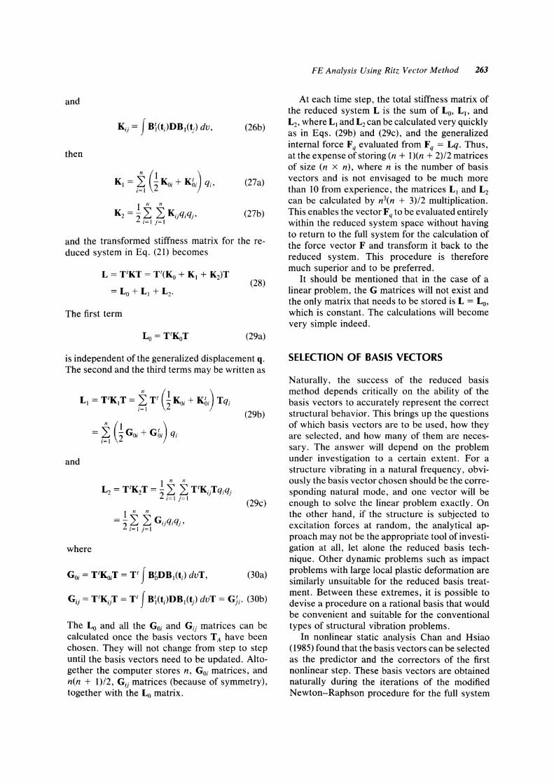
FIGURE 1 The finite element idealization of a cantilever beam.

0.90

0.80 / <:! 0.70 ~ c 0 0.60 'B " <;:::

" '0 0.50

~ 0.40

0.30

0.20

0.10

0.00

I Small defonnation' I I analysis

/ ~ ....-

\ ..--'

/ / ?

~ ,/ ~ ",. --Analytical

~ • Bathe -~

~ Current

.r Linear -

I.. 10

Load parameter q = PLJ/(EI)

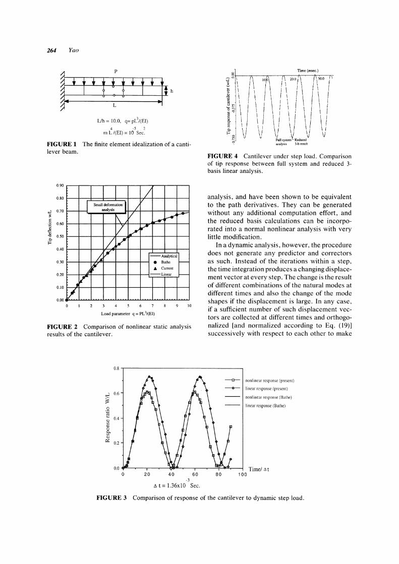
FIGURE 2 Comparison of nonlinear static analysis results of the cantilever.

8 Time (msec.)

--.0\ \

! \ , ~ \ I > I " \ '3 I L \ ~~

1\ I I I 0'"

\ I ~C? ! c \ I 0 \ I ~ ~ \ I 0. \/ \ I \ I \ I ~ \j V 0 V

~

d

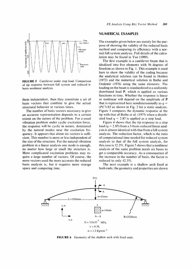
FIGURE 4 Cantilever under step load. Comparison of tip response between full system and reduced 3-basis linear analysis.

analysis, and have been shown to be equivalent to the path derivatives. They can be generated without any additional computation effort, and the reduced basis calculations can be incorporated into a normal nonlinear analysis with very little modification.

In a dynamic analysis, however, the procedure does not generate any predictor and correctors as such. Instead of the iterations within a step, the time integration produces a changing displacement vector at every step. The change is the result of different combinations of the natural modes at different times and also the change of the mode shapes if the displacement is large. In any case, if a sufficient number of such displacement vectors are collected at different times and orthogonalized [and normalized according to Eq. (19)] successively with respect to each other to make

0.8,---------------------,

...J 0.6

~ .2 e "' 0.4 '" t: o P. '" "' ~ 0.2

20 40 60 -3

~ t = 1.36xlO Sec.

80

nonlinear response (present)

linear response (present)

nonlinear response (Bathe)

linear response (Bathe)

Time/ ~t 100

FIGURE 3 Comparison of response of the cantilever to dynamic step load.

Full system analysis

\ result

I, , r I,

FIGURE 5 Cantilever under step load. Comparison of tip response between full system and reduced 6-basis nonlinear analysis.

them independent, then they constitute a set of basis vectors that combine to give the actual structural behavior at various times.

The number of basis vectors necessary to give an accurate representation depends to a certain extent on the nature of the problem. For a usual vibration problem under cyclic excitation force, the response will be cyclic in nature, dominated by the natural modes near the excitation frequency. It appears that about six vectors is sufficient. This number is more or less independent of the size ofthe structure. For the natural vibration problem in a linear analysis one mode is enough, no matter how large or small the structure is. More complicated excitation problems may require a large number of vectors. Of course, the more vectors used the more accurate the reduced basis analysis is, but it requires more storage space and computing time.


NUMERICAL EXAMPLES

The examples given below are mainly for the purpose of showing the validity of the reduced basis method and comparing its efficiency with a normal full system analysis. Full details of the calculation may be found in Yao (1989).

The first example is a cantilever beam that is idealized into five elements with 56 degrees of freedom as shown in Fig. 1. This example is used here to show the validity of the coding because the analytical solution can be found in Holden (1972) and the numerical solution in Bathe and Ozdemir (1976) using the same elements. The loading on the beam is standardized to a uniformly distributed load P, which is applied as various functions in time. Whether the response is linear or nonlinear will depend on the amplitude of P that is represented here nondimensionally as q =

(PL3)/ EI as shown in Fig. 2 for a static analysis. Figure 3 compares the dynamic response at the tip with that of Bathe et al. (1975) when a distributed load q = 2.85 is applied as a step load.

Figure 4 shows that the tip response to a step load (q = 2.85) from a 3-basis reduced linear analysis is almost identical with that from a full system analysis. The reduction factor, which is the ratio of computational time needed for reduced system analysis to that of the full system analysis, for this case is 12.2%. Figure 5 shows that a nonlinear analysis of the same problem needs six bases to get a comparable accuracy. As a consequence of the increase in the number of basis, the factor is reduced to only 42.3%.

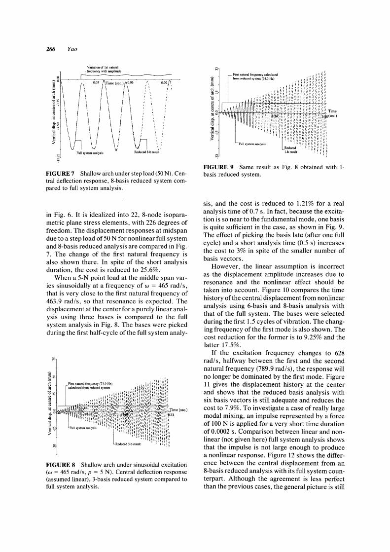
The next example is a shallow arch fixed at both ends; the geometry and properties are shown

h=43mm !'T""lil------L=lOOOmm-------''--------------F----1~

z,w

L a

~a=14mm A---A

X,U 9

E = 3.0x 10 MPa,

v = 0.38,

m=I.2Kg/mm 3

R=2928mm

FIGURE 6 Geometry of the shallow arch with fixed ends.

266 Yao

Variation of 1st natural frequency with amplitude .-------------

( \ 003 ,"rme (5ec,)/,\06

I \ I \ I \ I, \ /' \ I \ I \ I \

I \ I '

I I \ i \ !

" I' , , I '

009/~ I I

I I \ I \:

V~ \j \J ,Jl ') Full system analysis Reduced 8~b result

FIGURE 7 Shallow arch under step load (50 N). Central deflection response, 8-basis reduced system compared to full system analysis.

in Fig. 6. It is idealized into 22, 8-node isoparametric plane stress elements, with 226 degrees of freedom. The displacement responses at midspan due to a step load of 50 N for nonlinear full system and 8-basis reduced analysis are compared in Fig. 7. The change of the first natural frequency is also shown there. In spite of the short analysis duration, the cost is reduced to 25.6%.

When a 5-N point load at the middle span varies sinusoidally at a frequency of w = 465 rad/s, that is very close to the first natural frequency of 463.9 rad/s, so that resonance is expected. The displacement at the center for a purely linear analysis using three bases is compared to the full system analysis in Fig. 8. The bases were picked during the first half-cycle of the full system analy-

FIGURE 8 Shallow arch under sinusoidal excitation (w = 465 rad/s, p = 5 N). Central deflection response (assumed linear), 3-basis reduced system compared to full system analysis.

~

o

FIGURE 9 Same result as Fig. 8 obtained with 1-basis reduced system.

sis, and the cost is reduced to 1.21% for a real analysis time of 0.7 s. In fact, because the excitation is so near to the fundamental mode, one basis is quite sufficient in the case, as shown in Fig. 9. The effect of picking the basis late (after one full cycle) and a short analysis time (0.5 s) increases the cost to 3% in spite of the smaller number of basis vectors.

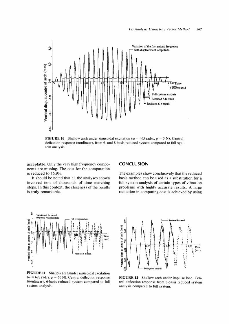
However, the linear assumption is incorrect as the displacement amplitude increases due to resonance and the nonlinear effect should be taken into account. Figure 10 compares the time history of the central displacement from nonlinear analysis using 6-basis and 8-basis analysis with that of the full system. The bases were selected during the first 1.5 cycles of vibration. The changing frequency of the first mode is also shown. The cost reduction for the former is to 9.25% and the latter 17.5%.

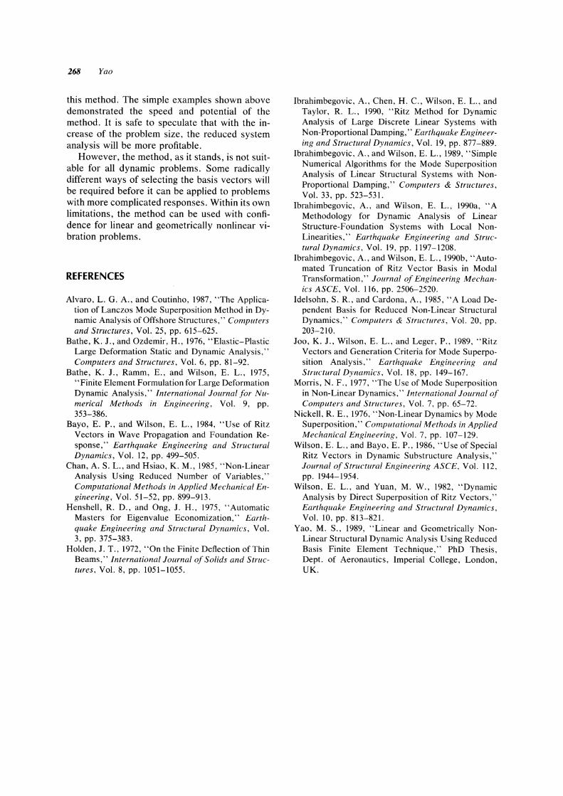
If the excitation frequency changes to 628 rad/s, halfway between the first and the second natural frequency (789.9 rad/s), the response will no longer be dominated by the first mode. Figure 11 gives the displacement history at the center and shows that the reduced basis analysis with six basis vectors is still adequate and reduces the cost to 7.9%. To investigate a case of really large modal mixing, an impulse represented by a force of 100 N is applied for a very short time duration of 0.0002 s. Comparison between linear and nonlinear (not given here) full system analysis shows that the impulse is not large enough to produce a nonlinear response. Figure 12 shows the difference between the central displacement from an 8-basis reduced analysis with its full system counterpart. Although the agreement is less perfect than the previous cases, the general picture is still

1\ ~ ~\

t-t-~r- r- r-

1\1 ~ \ .5 Xl( 1 2

\ o ~ ,


Variation of the first natural freq uency r- with displacement amplitude

I

IS

t:::::=

A ...... ,t\ f·

v.~ ., \3 V (

.5OTime lOOmsec.)

Full system anal ysis

ult Reduced 8-b res

Reduced 6-b result

FIGURE 10 Shallow arch under sinusoidal excitation (w = 465 rad/s, p = 5 N). Central deflection response (nonlinear), from 6- and 8-basis reduced system compared to full system analysis.

acceptable. Only the very high frequency components are missing. The cost for the computation is reduced to 16.9%.

It should be noted that all the analyses shown involved tens of thousands of time marching steps. In this context, the closeness of the results is truly remarkable.

Variation of Ist natural frequency with amplitude

FIGURE 11 Shallow arch under sinusoidal excitation (w = 628 rad/s, p = 60 N). Central deflection response (nonlinear), 6-basis reduced system compared to full system analysis.

CONCLUSION

The examples show conclusively that the reduced basis method can be used as a substitution for a full system analysis of certain types of vibration problems with highly accurate results. A large reduction in computing cost is achieved by using

r I,. :' ~

• I

1 ; ~ ; ~;

I, ,. ,', , " 1 ),

1

FIGURE 12 Shallow arch under impUlse load. Central deflection response from 8-basis reduced system analysis compared to full system.

268 Yao

this method. The simple examples shown above demonstrated the speed and potential of the method. It is safe to speculate that with the increase of the problem size, the reduced system analysis will be more profitable.

However, the method, as it stands, is not suitable for all dynamic problems. Some radically different ways of selecting the basis vectors will be required before it can be applied to problems with more complicated responses. Within its own limitations, the method can be used with confidence for linear and geometrically nonlinear vibration problems.

REFERENCES

Alvaro, L. G. A., and Coutinho, 1987, "The Application of Lanczos Mode Superposition Method in Dynamic Analysis of Offshore Structures," Computers and Structures, Vol. 25, pp. 615-625.

Bathe, K. J., and Ozdemir, H., 1976, "Elastic-Plastic Large Deformation Static and Dynamic Analysis," Computers and Structures, Vol. 6, pp. 81-92.

Bathe, K. J., Ramm, E., and Wilson, E. L., 1975, "Finite Element Formulation for Large Deformation Dynamic Analysis," International Journal for Numerical Methods in Engineering, Vol. 9, pp. 353-386.

Bayo, E. P., and Wilson, E. L., 1984, "Use of Ritz Vectors in Wave Propagation and Foundation Response," Earthquake Engineering and Structural Dynamics, Vol. 12, pp. 499-505.

Chan, A. S. L., and Hsiao, K. M., 1985, "Non-Linear Analysis Using Reduced Number of Variables," Computational Methods in Applied Mechanical Engineering, Vol. 51-52, pp. 899-913.

Henshell, R. D., and Ong, J. H., 1975, "Automatic Masters for Eigenvalue Economization," Earthquake Engineering and Structural Dynamics, Vol. 3, pp. 375-383.

Holden, J. T., 1972, "On the Finite Deflection of Thin Beams," International Journal of Solids and Structures, Vol. 8, pp. 1051-1055.

Ibrahimbegovic, A., Chen, H. C., Wilson, E. L., and Taylor, R. L., 1990, "Ritz Method for Dynamic Analysis of Large Discrete Linear Systems with Non-Proportional Damping," Earthquake Engineering and Structural Dynamics, Vol. 19, pp. 877-889.

Ibrahimbegovic, A., and Wilson, E. L., 1989, "Simple Numerical Algorithms for the Mode Superposition Analysis of Linear Structural Systems with NonProportional Damping," Computers & Structures, Vol. 33, pp. 523-531.

Ibrahimbegovic, A., and Wilson, E. L., 1990a, "A Methodology for Dynamic Analysis of Linear Structure-Foundation Systems with Local NonLinearities," Earthquake Engineering and Structural Dynamics, Vol. 19, pp. 1I97-1208.

Ibrahimbegovic, A., and Wilson, E. L., 1990b, "Automated Truncation of Ritz Vector Basis in Modal Transformation," Journal of Engineering Mechanics ASCE, Vol. 116, pp. 2506-2520.

Idelsohn, S. R., and Cardona, A., 1985, "A Load Dependent Basis for Reduced Non-Linear Structural Dynamics," Computers & Structures, Vol. 20, pp. 203-210.

Joo, K. J., Wilson, E. L., and Leger, P., 1989, "Ritz Vectors and Generation Criteria for Mode Superposition Analysis," Earthquake Engineering and Structural Dynamics, Vol. 18, pp. 149-167.

Morris, N. F., 1977, "The Use of Mode Superposition in Non-Linear Dynamics," International Journal of Computers and Structures, Vol. 7, pp. 65-72.

Nickell, R. E., 1976, "Non-Linear Dynamics by Mode Superposition," Computational Methods in Applied Mechanical Engineering, Vol. 7, pp. 107-129.

Wilson, E. L., and Bayo, E. P., 1986, "Use of Special Ritz Vectors in Dynamic Substructure Analysis," Journal of Structural Engineering ASCE, Vol. 1I2, pp. 1944-1954.

Wilson, E. L., and Yuan, M. W., 1982, "Dynamic Analysis by Direct Superposition of Ritz Vectors," Earthquake Engineering and Structural Dynamics, Vol. 10, pp. 813-821.

Yao, M. S., 1989, "Linear and Geometrically NonLinear Structural Dynamic Analysis Using Reduced Basis Finite Element Technique," PhD Thesis, Dept. of Aeronautics, Imperial College, London, UK.

International Journal of

AerospaceEngineeringHindawi Publishing Corporationhttp://www.hindawi.com Volume 2010

RoboticsJournal of

Hindawi Publishing Corporationhttp://www.hindawi.com Volume 2014


Active and Passive Electronic Components

Control Scienceand Engineering

Journal of



RotatingMachinery


Hindawi Publishing Corporation http://www.hindawi.com

Journal ofEngineeringVolume 2014

Submit your manuscripts athttp://www.hindawi.com

VLSI Design



Shock and Vibration


Civil EngineeringAdvances in

Acoustics and VibrationAdvances in



Electrical and Computer Engineering

Journal of

Advances inOptoElectronics

Hindawi Publishing Corporation http://www.hindawi.com

Volume 2014

The Scientific World JournalHindawi Publishing Corporation http://www.hindawi.com Volume 2014

SensorsJournal of


Modelling & Simulation in EngineeringHindawi Publishing Corporation http://www.hindawi.com Volume 2014


Chemical EngineeringInternational Journal of Antennas and

Propagation




Navigation and Observation



DistributedSensor Networks


of nonlinear structural dynamic engineering brunei

Documents