OF GENES AND MACHINES: APPLICATION OF A COMBINATION OF MACHINE LEARNING TOOLS TOASTRONOMY DATA SETS

S. Heinis1, S. Kumar

1, S. Gezari

1, W. S. Burgett

2, K. C. Chambers

2, P. W. Draper

3, H. Flewelling

2, N. Kaiser

2,

E. A. Magnier2, N. Metcalfe

3, and C. Waters

2

1 Department of Astronomy, University of Maryland, College Park, MD, USA2 Institute for Astronomy, University of Hawaii at Manoa, Honolulu, HI 96822, USA3 Department of Physics, Durham University, South Road, Durham DH1 3LE, UK

Received 2015 August 17; accepted 2016 March 2; published 2016 April 13

ABSTRACT

We apply a combination of genetic algorithm (GA) and support vector machine (SVM) machine learningalgorithms to solve two important problems faced by the astronomical community: star–galaxy separation andphotometric redshift estimation of galaxies in survey catalogs. We use the GA to select the relevant features in thefirst step, followed by optimization of SVM parameters in the second step to obtain an optimal set of parameters toclassify or regress, in the process of which we avoid overfitting. We apply our method to star–galaxy separation inPan-STARRS1 data. We show that our method correctly classifies 98% of objects down to =i 24.5P1 , with acompleteness (or true positive rate) of 99% for galaxies and 88% for stars. By combining colors with morphology,our star–galaxy separation method yields better results than the new SExtractor classifier spread_model, inparticular at the faint end ( >i 22P1 ). We also use our method to derive photometric redshifts for galaxies in theCOSMOS bright multiwavelength data set down to an error in ( )+ z1 of s = 0.013, which compares well withestimates from spectral energy distribution fitting on the same data (s = 0.007) while making a significantlysmaller number of assumptions.

Key words: methods: numerical

1. INTRODUCTION

Astronomy has witnessed an ever-increasing deluge of dataover the past decade. Future surveys will gather very largeamounts of data daily that will require on-the-fly analysis tolimit the amount of data that can be stored or analyzed and toallow timely discoveries of candidates to be followed up:examples are Euclid (Laureijs et al. 2011, 100 GB per day),WFIRST (Spergel et al. 2015, 1.3 TB per day), and the LargeSynoptic Survey Telescope (Ivezic et al. 2008, 10 TB per day).The evolution of the type, volume, and cadence of theastronomical data requires the advent of robust methods thatwill enable a maximal rate of extraction of information from thedata. Thus, for a given problem, one needs to make sure all therelevant information is made available in the first step, followedby the use of a suitable method that is able to narrow down theimportant aspects of the data. This can be done both for featureselection and for noise filtering.

In machine learning parlance, the tasks required can bedesignated as classification tasks (derive a discrete value: starversus galaxy, for instance) or regression tasks (derive acontinuous value: photometric redshift, for instance.) Methodsfor classification or regression usually are of two kinds:physically motivated or empirical.4 Physically motivatedmethods use templates built from previously observed data,like star or galaxy spectral energy distributions (SEDs), forinstance, in the case of determining photometric redshifts. Theyalso attempt to include as much knowledge as we have of theprocesses involved in the problem at stake, such as priorinformation. Physically motivated methods seem more appro-priate than empirical, but the very fact that they require a goodknowledge of the physics involved might be an important

limitation. Indeed, our knowledge of a number of the processesinvolved in shaping the SEDs of galaxies, for instance, is stillquite limited (e.g., Conroy et al. 2010, and references therein),whether it is about the processes driving star formation, dustattenuation laws, initial mass function, star formation history,or active galactic nucleus (AGN) contribution. Hence, choicesneed to be made: either make a number of assumptions, inorder to reduce the number of free parameters, or decide to bemore inclusive and add more parameters, but at the cost ofpotential degeneracies. Physically motivated methods are alsousually limited in the way they treat the correlation between theproperties of the objects because the only correlations takeninto account are those included in the models used and mightnot reflect all of the information contained in the data.On the other hand, empirical methods require few or no

assumptions about the physics of the problem. The goal of anempirical method is to build a decision function from the datathemselves. The quality of the generalization of the results to afull data set depends of course on the representativeness of thetraining sample. We note, however, that the question of thegeneralization also applies to physically motivated methodsbecause they are also validated on the training data.Depending on the methods used, transformations may need

to be effected before the method is applied; for example, in thecase of support vector machines (SVM; e.g., Boser et al. 1992;Cortes & Vapnik 1995; Vapnik 1995, 1998; Smola &Schölkopf 1998; Duda et al. 2001), linear separability ispresumed, thereby requiring nonlinearly separable or regres-sible data to be kernel transformed to enable this.A challenge with empirical methods is that with growing

numbers of input parameters, it becomes prohibitive in terms ofCPU time to use all of them. It can also be counterproductive tofeed the machine learning tool with all of these parametersbecause some of them might either be too noisy or not bring

The Astrophysical Journal, 821:86 (10pp), 2016 April 20 doi:10.3847/0004-637X/821/2/86© 2016. The American Astronomical Society. All rights reserved.

4 Formalisms that blend physically motivated and empirical methods havebeen proposed; see, e.g., Budavári (2009).

1

any relevant information to the specific problem being tackled.Moreover, high-dimensional problems suffer from being overfitby machine learning methods (Cawley & Talbot 2010), therebyyielding high-dimensional nonoptimal solutions. This requiressubselection of relevant variables from a large N-dimensionalspace (with N potentially close to 1000). This task itself canalso be achieved using machine learning tools. Here wepresent, to our knowledge, the first application to astronomy ofthe combination of two machine learning techniques: geneticalgorithms (GA; e.g., Steeb 2014) for selecting relevantfeatures, followed by SVMs to build a decision–rewardfunction. GAs alone have already been used in astronomy,for instance, in the study of orbits of exoplanets and the SEDsof young stellar objects (Cantó et al. 2009), the analysis ofSN Ia data (Nesseris 2011), the study of star-formation andmetal-enrichment histories of a resolved stellar system (Smallet al. 2013), the detection of globular clusters from HubbleSpace Telescope (HST) imaging (Cavuoti et al. 2014), andphotometric redshift estimation (Hogan et al. 2015). At thesame time, SVMs have been extensively used to solve anumber of problems, such as object classification (Zhang &Zhao 2004), the identification of red variable sources (Woźniaket al. 2004), photometric redshift estimation (Wadadekar 2005),morphological classification (Huertas-Company et al. 2011),and parameter estimation for Gaia spectrophotometry (Liuet al. 2012). We note also that the combination of GA andSVM has already been used in a number of fields, such ascancer classification (e.g., Huerta et al. 2006; Albdaet al. 2007), chemistry (e.g., Fatemi & Gharaghani 2007),and bankruptcy prediction (e.g., Min et al. 2006). We do notattempt here to provide the most optimized results from thiscombination of methods. Rather, we present a proof of conceptthat shows that GA and SVM yield remarkable results whencombined, as opposed to using the SVM as a standalone tool.

In this paper, we focus on two tasks frequently seen in largesurveys: star–galaxy separation and the determination ofphotometric redshifts of distant galaxies. Star–galaxy separa-tion is a classification problem that has usually beenconstrained purely from the morphology of the objects (e.g.,Kron 1980; Bertin & Arnouts 1996; Stoughton et al. 2002). Anumber of studies have used color information with templatefitting to separate stars from galaxies (e.g., Fadely et al. 2012).On top of these two common approaches, good results havebeen obtained by feeding morphology and colors to machinelearning techniques (e.g., Vasconcellos et al. 2011; Saglia et al.2012; Kovács & Szapudi 2015). Our goal here is to extend thestar–galaxy separation to faint magnitudes, where the morphol-ogy is not as reliable. We apply here the combination of GAwith SVM to star–galaxy separation in the Pan-STARRS1(PS1) Medium Deep Survey (Kaiser et al. 2010; Tonryet al. 2012; Rest et al. 2014).

On the other hand, the determination of photometricredshifts is a well-studied problem of regression that has beendealt with using a variety of methods, including template fitting(e.g., Arnouts et al. 1999; Benítez 2000; Brammer et al. 2008;Ilbert et al. 2009), cross-correlation functions (Rahmanet al. 2015), random forests (Carliles et al. 2010), neuralnetworks (Collister et al. 2007), polynomial fitting (Connollyet al. 1995), and symbolic regression (Krone-Martinset al. 2014). We apply the GA-SVM to the zCOSMOS brightsample (Lilly et al. 2007).

The outline of this paper is as follows. In Section 2 wepresent the data to which we apply our methods and thetraining sets we use: PS1 and zCOSMOS bright. In Section 3we briefly describe our methods; we include a more detaileddescription of SVM in an Appendix. We present our results inSection 4 and finally list our conclusions.

2. DATA

We perform star–galaxy separation in PS1 Medium Deepdata (Section 2.1), using a training set built from COSMOSAdvanced Camera for Surveys (ACS) imaging (Section 2.2.1).We then derive photometric redshifts for the zCOSMOS brightsample (Section 2.2.2).

2.1. Pan-STARRS1 Data

The Pan-STARRS1 survey (Kaiser et al. 2010) surveyedthree-quarters of the northern hemisphere (d > - 30 ) in fivefilters: gP1, rP1, iP1, zP1, and yP1 (Tonry et al. 2012). In addition,PS1 has obtained deeper imaging in 10 fields (amounting to80 deg2) called the Medium Deep Survey (Tonry et al. 2012;Rest et al. 2014). We use here data in the MD04 field, whichoverlap the COSMOS survey (Scoville et al. 2007).We use our own reduction of the PS1 data in the Medium

Deep Survey. We use the image stacks generated by the ImageProcessing Pipeline (Magnier 2006) and also the CFHT u-banddata obtained by E. Magnier as follow-up of the Medium Deepfields. We have at hand six bands: uCFHT, gP1, rP1, iP1, zP1, andyP1. We perform photometry using the following steps,considering PS1 skycell as the smallest entity: (1) resample(using SWarp, Bertin et al. 2002) the u-band images to the PS1resolution, and register all images; (2) for each band, fit thepoint-spread function (PSF) to a Moffat function and matchthat PSF to the worst PSF in each skycell; (3) using these PSF-matched images, we derive a c2 image (Szalay et al. 1999); (4)we perform photometry using the SExtractor dual mode(Bertin & Arnouts 1996), detecting objects in the c2 image andmeasuring the fluxes in the PSF-matched images: the Kron-likeapertures are defined from the c2 image and hence are the sameover all bands; (5) for each detection, we measure spread_-model in each band on the original, non-PSF-matched images.We consider here Kron magnitudes, which are designed tocontain ∼90% of the source light, regardless of being from apoint-source star or an extended galaxy.Here, spread_model (Soumagnac et al. 2013) is a

discriminant between the local PSF, measured with PSFEx(Bertin 2011), and a circular exponential model of scale lengthFWHM 16 convolved with that PSF. This discriminant hasbeen shown to perform better than SExtractor’s previousmorphological classifier, class_star.

2.2. COSMOS Data

2.2.1. Star–Galaxy Classification Training Set

We use the star–galaxy classification from Leauthaud et al.(2007) derived from high-spatial-resolution HST imaging (inthe F W814 band) as our training set for star–galaxyclassification. They separate stars from galaxies based on theirSExtractor mag_auto and mu_max (peak surface bright-ness above surface level). By comparing the derived stellarcounts with the models of Robin et al. (2007), Leauthaud et al.(2007) showed that the stellar counts are in excellent agreement

2

The Astrophysical Journal, 821:86 (10pp), 2016 April 20 Heinis et al.

with the models for < <F W20 814 25. We perform here star–galaxy separation down to =i 24.5P1 .

2.2.2. Spectroscopic Redshift Training Set

We use data taken as part of the COSMOS survey (Scovilleet al. 2007). We focus here on objects with spectroscopicredshifts obtained during the zCOSMOS bright campaign(Lilly et al. 2007, <i 22.5). We use the photometry obtained in25 bands by various groups in broad optical and near-infraredbands (Capak et al. (2007, u

*

, BJ, VJ, +g , +r , +i , +z , Ks), innarrow bands (Taniguchi et al. 2007, NB816; Ilbert et al. 2009,NB711), and in intermediate bands (Ilbert et al.2009, IA427,IA464, IA505, IA574, IA709, IA827, IA484, IA527, IA624,IA679, IA738, IA767). We also use IRAC1 and IRAC2photometry (Sanders et al. 2007). We consider here onlyobjects with good redshift determination (confidence class: 3.5and 4.5), <z 1.5 (which yields 5807 objects) and measuredmagnitudes for all the bands listed above, which finally leavesus with 5093 objects. We do not use objects with otherconfidence-class values because the spectroscopic redshifts canbe erroneous in at least 15% of cases (O. Ilbert 2016, privatecommunication).

3. METHODS

We present here the two machine learning methods we use inthis work: GAs are used to select the relevant features, andSVMs are used to predict the property of interest using thesefeatures.

3.1. Genetic Algorithms

GAs (e.g., Steeb 2014) apply the basic premise of genetics tothe evolution of solution sets of a problem until they reachoptimality. The definition of optimality itself is debatable, butthe general idea is to use a reward function to direct theevolution. That is, we evolve solution sets of parameters (orgenes) known as organisms through several generationsaccording to some predefined evolutionary reward function.The reward function may be a goodness of fit or a functionthereof that may take into account more than just the goodnessof fit. For example, one may choose to determine subsets ofparameters that optimize c2 or likelihood, Akaike informationcriteria, energy functions, or entropy. The lengths of the firstgeneration of organisms are chosen to range from the minimumexpected dimensionality of the parameter space (which can beone) to the maximum expected dimensionality of thecovariance.

The fittest organisms in a particular generation are then givenhigher probabilities of being chosen to be the parents forsuccessive generations using a roulette selection method basedon their fitnesses. Parents are then crossbred using acustomized procedure; in our method we first choose thelengths of the children to be based on a tapered distributionwhere the taper depends on the fitnesses of the parents. Thatway the length of the child is closer to that of the fitter parent.The child is then populated using the genes of both parents,where genes that are present in both parents are given twice theweight of genes that are only present in one parent. The idea isthat the child should, with a greater probability, contain genesthat are present in both parents, as opposed to the onescontained in only one of them. This process iterativelyproduces fitter children in successive generations and is

terminated when no further improvement in the averageorganism quality is seen. Like in biological genetics, we alsointroduce a mutation in the genes with constant probability.The genes that are chosen to be mutated are replaced with anyof the genes that are not part of either parent, with a uniformprobability of choosing from the remaining genes. This allowsfor genes that are not part of the current gene pool to beexpressed. The conceptual simplicity of GA combined withtheir evolutionary analogy as applied to some of the hardestmultiparameter global optimization problems makes themhighly sought after.

3.2. Support Vector Machines

SVM (e.g., Boser et al. 1992; Cortes & Vapnik 1995;Vapnik 1995, 1998; Smola & Schölkopf 1998; Dudaet al. 2001) is a machine learning algorithm that constructs amaximum-margin hyperplane to separate linearly separablepatterns. SVM is especially efficient in high-dimensionalparameter spaces, where separating two classes of objects is ahard problem, and performs with best-case complexityn nparameters samples

2 . Where the data are not linearly separable,a kernel transformation can be applied to map the originalparameter space to a higher-dimension feature space where thedata become linearly separable. For both problems we attemptto solve in this paper, we use a Gaussian radial basis functionkernel, defined as

( ) ( ∣∣ ∣∣ ) ( )g¢ = - - ¢K x x x x, exp . 12

Another advantage of using SVM is that there areestablished guarantees of their performance, which have beenwell documented in the literature. Also, the final classificationplane is not affected by local minima in the classification orregression statistic, which other methods based on least squaresor maximum likelihood may not guarantee. For a detaileddescription of SVM, please refer to Smola & Schölkopf (1998)and Vapnik (1995, 1998). We use here the Pythonimplementation within the Scikit-learn (Pedregosaet al. 2011) module.

3.3. Optimization Procedure

We combine the GA and SVM to select the optimal set ofparameters that enables one to classify objects or derivephotometric redshifts. In either case, we first gather all inputparameters and then build color combinations from allavailable magnitudes. We also consider here transformationsof the parameters, namely their logarithm and exponential ontop of their catalog values, which we name “linear” afterward,in order to capture nonlinear dependencies on the parameters.Note that any transformation could be used; we limitedourselves to log and exp for the sake of simplicity for thisfirst application. This way, the rate of change of the dependentparameter as a function of the independent parameter inquestion is more accurately captured, and dependencies onmultiple transformations of the same variable can also becaptured. To eliminate scaling issues in transformed spaces, wetransform all independent parameters to between −1 and 1. Theoptimization is then performed in the following two stepsiteratively until the end criterion or convergence criterion ismet: selection of the relevant set of features in the first, andautomatic optimization of SVM parameters to yield optimalclassification/regression given the parameters. For SVMclassification, the true positive rate is used as the fitness

3

The Astrophysical Journal, 821:86 (10pp), 2016 April 20 Heinis et al.

function. For SVM regression, a custom fitness function basedon the problem at hand is chosen. For example, for SVMregressions on the photometric redshift we use

( )å

-⎜ ⎟⎛⎝

⎞⎠

1. 2

i

z z

z

2i i

i

phot spec

phot

Once the fitness of all organisms has been evaluated, a newgeneration of the same size as the parent generation is createdusing roulette selection. The GA then runs until it reaches apredefined stopping criterion. We use here the posteriordistribution of the parameters. We stop the GA when allparameters have been used at least 10 times. We also use theposterior distribution to choose the optimal set of parameters.Various schemes can be defined. For our application, werestrict ourselves to characterizing the posterior distribution byits mean μ and standard deviation σ (see Figure 1). Weconsider here all parameters that appear more than m s+ orm s+ 2 times in the posterior distribution, depending on whichof our results change significantly. For instance, in the case ofphotometric redshifts, the mean of the posterior distribution ism = 13.8, and the standard deviation is s = 10.4; we keep allparameters that occur more than 24 times in the posteriordistribution when using the m s+ criterion.

3.3.1. SVM Parameter Optimization

SVM are not “black boxes” but come with a well-definedformalism and free parameters to be adjusted. For thisapplication, we use the νSVM version of the algorithm, whichallows us to control the fractional error and the lower limit onthe fraction of support vectors used. We use here n = 0.1. Inthe case of classification (star–galaxy separation), we are then

left with only one free parameter, the inverse of the width of theGaussian kernel, γ (Equation (1)). In the case of regression(photometric redshifts), we have an additional free parameter,the trade-off parameter C (see Appendix).If not used with caution, machine learning methods can lead

to overfitting: the decision function is biased by the trainingsample and will not perform well on other samples. In order toavoid overfitting and optimize the values of γ and C, weperform a 10-fold cross-validation, in which we divide thesample into 10 subsets, and we then perform classification orregression for each subset after training on the nine othersubsets. We perform this cross-validation for a grid of γ and Cvalues. In the case of SVM, the overfitting can be measured bythe fraction of objects used as support vectors, fSV. If ~f 1SV ,most of the training sample is used as support vectors, whichwill lead to poor generalization. For each iteration, we also getfSV, in order to include it in our cost function. For bothapplications, we minimize a custom cost function thatoptimizes the quality of the classification or regression,and fSV.

4. RESULTS

4.1. Star–Galaxy Separation

We use as inputs to the GA feature selection step allmagnitudes available for the PS1 data set: uCFHT, gP1, rP1, iP1,zP1, and y ;P1 the spread_model values derived from each ofthese bands; and the ellipticity measured on the c2 image, withall colors. We also included a few quantities determined byrunning the code lephare on these data: the photometricredshift and the ratios of the minimum c2 using galaxy, star,and quasar templates: c cgalaxy

2star2 , c cgalaxy

2quasar2 , and

c cquasar2

star2 . Including the transformations of these parameters

yields 96 input parameters to the GA-SVM feature selectionprocedure.The parameters selected by the GA with occurrence larger

than m s+ times in the posterior distribution are listed in

Figure 1. Example of posterior distribution for the parameters obtained fromthe GA-SVM. This posterior distribution was derived for the application tophotometric redshifts (Section 4.2). The red solid line shows the averageoccurrence of the parameters, the dashed blue line the occurrence at the meanplus one standard deviation, and the dotted blue line the occurrence at the meanplus two standard deviations. We use here all parameters that appear moretimes than the mean plus one standard deviation in the posterior distribution.

Table 1Star–Galaxy Separation: GA Output Parameters

Parameter Transform Occurrence Thresholda

uCFHT log m s+rP1 lin m s+rP1 log m s+ 2spread_model_g exp m s+spread_model_r lin m s+ 2spread_model_r log m s+ 2spread_model_i exp m s+ 2

-u gCFHT P1 lin m s+-u zCFHT P1 lin m s+-u yCFHT P1 lin m s+ 2

-g yP1 P1 log m s+-r yP1 P1 exp m s+-i yP1 P1 lin m s+-z yP1 P1 exp m s+

zphot lin m s+

Note.a Here, m s+ indicates that the parameter occurred at least m s+ times inthe posterior distribution of the GA, while m s+ 2 indicates that the parameteroccurred m s+ 2 times.

4

The Astrophysical Journal, 821:86 (10pp), 2016 April 20 Heinis et al.

Table 1. We also indicate the parameters whose occurrence islarger than m s+ 2 times. The 15 selected parameters includespread_model derived in gP1, rP1, and iP1, but are dominatedby colors (seven of 15). Using the parameters occurring morethan m s+ 2 yields similar results, although with significantoverfitting.

In order to quantify the quality of the star–galaxy separation,we use the following definitions for the completeness c and thepurity p:

( )=+

cn

n m3g

g

g g

( )=+

pn

n m4g

g

g s

where nx is the number of objects of class x correctly classified,and mx is the number of objects of class x misclassified. Thesame definition holds for the star completeness and purity.

Based on these definitions, in the case of star–galaxyseparation, we use this as the cost function:

( )

=-

+-

+-

+-

+-

⎜ ⎟⎛⎝⎜

⎞⎠⎟

⎛⎝

⎞⎠

⎛⎝⎜

⎞⎠⎟

⎛⎝⎜

⎞⎠⎟

⎛⎝⎜

⎞⎠⎟

Jc c p

p f

1

0.005

1

0.005

1

0.005

1

0.005

0.1

0.01. 5

g2

s2

g2

s2

SV2

In other words, we choose here to optimize the averagecompleteness and purity for stars and galaxies and also penalizehigh fSV, which amounts to penalizing high fractional errors,and overfitting as well. Other optimization schemes can beadopted. We perform the optimization over the only SVM freeparameter here, the inverse of the width of the Gaussian kernel,

γ. We use a grid search using a log-spaced binningfor g< <0.01 10.We show in Figure 2 the spread_model derived in the

PS1 i band as a function of iP1. Figure 2 shows thatspread_model enables us to recover a star sequence downto ~i 22P1 . At fainter magnitudes, morphology alone is notable to accurately separate stars from galaxies at the PS1angular resolution. The color coding shows the result of theGA-SVM classification. We classify objects down to

=i 24.5P1 . We choose this limit because the completeness ofthe PS1 data drops significantly beyond 24.5, and also becausethe training set we use is valid down to =F W814 25. Figure 1suggests that the GA-SVM is able to recover the classificationat bright magnitudes but also to extend it at the faint end. Welist in Table 2 the percentage of objects classified correctly. Ourmethod correctly classifies 97% of the objects down to

=i 24.5P1 . We can compare our results to those from thePS1 photometric classification server (Saglia et al. 2012),which used SVM on bright objects using PS1 photometry.They obtained 84.9% of stars correctly classified down to

=i 21P1 and 97% of galaxies down to = 20P1 . Our methodenables us to improve upon those, as we get 88.6% of starscorrectly classified and 99.3% of galaxies correctly classified inthe same magnitude range.We examine in more detail in Figures 3 and 4 the colors of

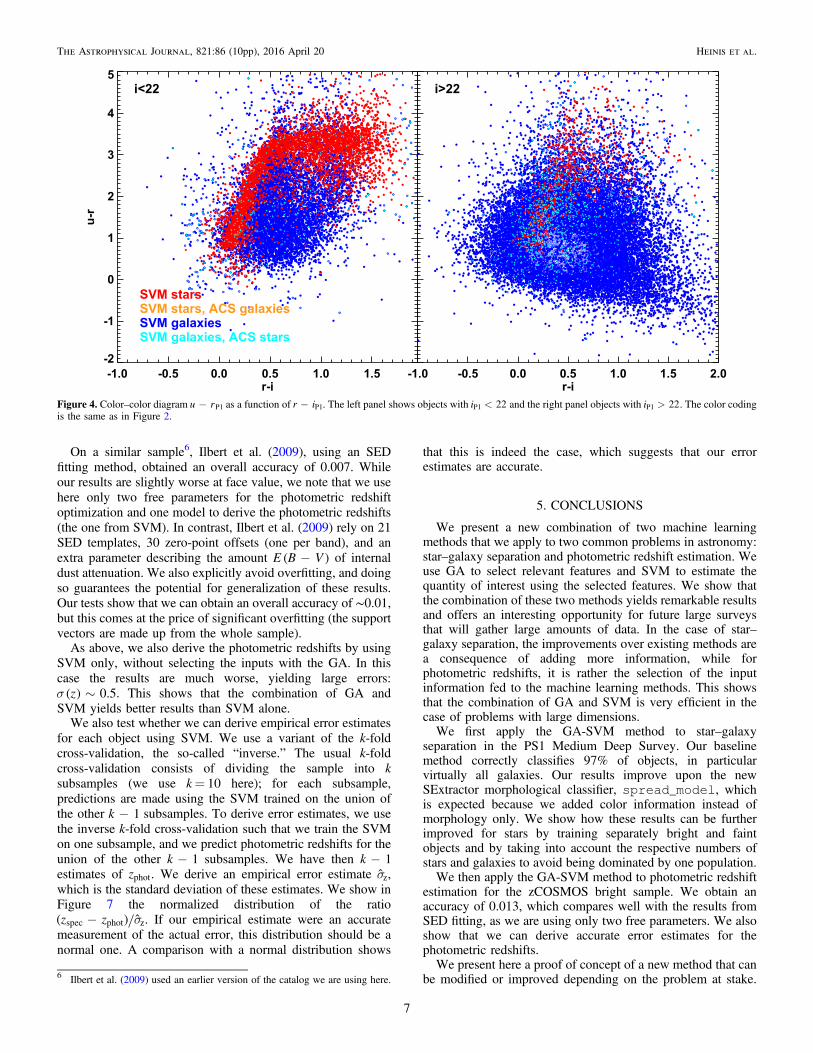
the objects. These figures show that the bulk of stars that aremisclassified as galaxies are at the faint end, i 22, and thatthese objects are in regions where the colors of stars andgalaxies are similar. Galaxies misclassified as stars are brighter,<i 22, but again are in regions where the colors of stars and

galaxies overlap. There are also a handful of very bright starsmisclassified as galaxies, in a domain where the galaxysampling is very poor. Finally, we classify as galaxies a fewstars showing colors at the outskirts of the color distributions.These objects might be misclassified by the ACS photometry,or the color might be significantly impacted by photometricscatter.We show in Figure 5 the completeness (left) and purity

(right) of our classifications as a function of iP1.We derive the completeness and purity for each cross-

validation subset and show in Figure 5 the average and as errorbars the standard deviation. Most of the features of ourclassification seen in Figure 5 are due to the fact that thetraining sample is unbalanced at the bright end and the faintend: at the bright end, stars outnumber the galaxies, and theother way around at the faint end. At the bright end ( <i 16P1 ,which is also within the saturation regime), the completeness ishigher for stars than for galaxies, while noisy because of smallstatistics. Some bright galaxies are misclassified as stars. At thefaint end ( >i 22P1 ), the star completeness decreases because

Figure 2. SExtractor morphological classifier spread_model measured inthe PS1 i band as a function of iP1. We also show the result of our baselineclassification (training on all objects): red points show objects classified as starsby the GA-SVM, and blue points show objects classified as galaxies. Orangeand cyan points show misclassified objects: orange points are galaxiesaccording to the catalog of Leauthaud et al. (2007) classified as stars, and cyanpoints are stars classified as galaxies.

Table 2Star–Galaxy Separation: Performance

Type GA-SVM alla GA-SVM Bright/Faintb spread_modelc

All types 97.4 98.1 92.7Galaxies 99.8 99.2 94.5Stars 74.5 88.5 75.9

Notes. Percentage of correctly classified objects for each method:a Training and prediction on the full sample.b Training and prediction on bright and faint objects separately.c SExtractor spread_model method.

5

The Astrophysical Journal, 821:86 (10pp), 2016 April 20 Heinis et al.

some stars are classified as galaxies. The impression given byFigure 5 is striking, as the star completeness decreases to 0 at

~i 24P1 . Note, however, that the stars represent only 3% of theoverall population at this flux level (Leauthaud et al. 2007).The purity shows a similar behavior at the bright end. At thefaint end, however, the purity of the stars is larger than 0.85 for

i 23P1 . For galaxies, both completeness and purity are lowerthan 0.8 at the bright end ( <i 18P1 ), but the number of galaxiesis small at these magnitudes. At >i 18P1 , completeness andpurity are independent of magnitude down to =i 24.5P1 andlarger than 0.95.

We compare these results to the classification obtained withspread_model derived in the iP1 band. We determine asingle cut in spread_model_i using its distribution forreference stars and galaxies. Our cut is the value ofspread_model_i such that

spread model i spread model i( ∣ ) ( ∣ )=p g _ _ p s _ _ . Weshow in Figure 5 the completeness and purity obtained withspread_model_i as dotted lines. For iP122, the resultsfrom spread_model_i and our method are similar: at thePS1 resolution, point sources and extended objects are welldiscriminated in this magnitude range. At >i 22P1 , ourbaseline method performs better, in particular for galaxies,which is expected as we add color information. While thegalaxies’ purity is similar for both methods, the completenessobtained with spread_model_i drops to 0.75 at =i 24.5P1 ,but our method yields a completeness consistent with 1 downto this magnitude. For stars, the purity obtained with the twomethods is similar. However, the completeness we obtain dropsfaster than that obtained with spread_model_i. In order tosee whether we can improve our baseline method, we optimizethe SVM parameters independently in two magnitude ranges:

<i 22P1 and >i 22P1 . Because galaxies at the faint endoutnumber stars by several orders of magnitude, we add anextra free parameter for the optimization at >i 22P1 , which

attempts to correct this sampling issue. In practice, we use allstars available, but only a fraction of the galaxies available,from one to 10 times the number of stars. The results obtainedare shown in solid lines on Figure 5. The results for galaxies arevirtually unchanged compared to our baseline method. Forstars, we are able to improve at the faint end, where the purityis better than that obtained with spread_model_ifor <i 23P1 .As a final check, we also derive the star–galaxy separation

by using SVM only, without selecting the inputs with the GA.The results are only marginally different. We note, however,that a parameter space with lower dimensions is less prone tooverfitting with machine learning methods. On the other hand,even with similar results, a SVM-based star–galaxy separationwith a smaller number of input parameters is more likely togeneralize properly.

4.2. Photometric Redshifts

We used 978 input parameters as inputs for the GA-SVMoptimization procedure: all magnitudes and colors availablefrom the COSMOS data set and the transformations of theseparameters, as described in Section 3.3. Hereafter we considerthe parameters that appear at least m s+ 1 times in theposterior distribution, so we are left with 131 parameters. Theparameters retained by the GA-SVM are dominated by colors(82%, 108/131), in particular colors involving intermediateand narrow bands (71%, 93/131). Using the parameters thatappear m s+ 2 times in the GA posterior distribution yields 45parameters, with similar proportions of colors and intermediateand narrow bands. This is in line with the conclusions ofstudies using SED fitting methods, which show that includingnarrow and intermediate bands improves significantly theestimation of photometric redshifts (e.g., Ilbert et al. 2009).We quantify the errors on photometric redshifts as( ) ( ) ( )= - +z z z zerr 1spec phot spec spec , using as a measure of

global accuracy σ, the normalized median absolute deviation,defined as

( )s = *z 1.4826 median (∣ ( ) ( ( ))∣)-z zerr median errspec spec .We define the following cost function for the SVM

optimization:

( ) ( )s=

-+

-⎜ ⎟⎛⎝

⎞⎠

⎛⎝⎜

⎞⎠⎟J

z f0.005

0.0001

0.1

0.01. 6

2SV

2

We perform the optimization over the two SVM freeparameters available here, γ and the trade-off parameter C. Weuse a grid search using a log-spaced binning for g< <0.01 10and < <C0.01 500.We compare in Figure 6 the spectroscopic and photometric

redshifts. We obtain an overall accuracy of 0.013.5 Thepercentage of outliers, defined as objects with∣ ( )∣ >zerr 0.15spec , is below 1%. The average error (bias) isequivalent to zero; our results do not show any significant biasas a function of redshift. At high redshifts ( >z 1) thespectroscopic sampling is small, so the model is lessconstrained. Using the parameters that appear m s+ 2 timesin the GA-SVM posterior distribution yields similar results( ( )s =z 0.014), which shows that by using three times fewerparameters, the same accuracy can be achieved.

Figure 3. Color–magnitude diagram -g iP1 as a function of iP1. The colorcoding is the same as in Figure 2.

5 Using objects with spectroscopic confidence class <CC3 5 yieldssimilar results with an accuracy of ( )s =z 0.015.

6

The Astrophysical Journal, 821:86 (10pp), 2016 April 20 Heinis et al.

On a similar sample6, Ilbert et al. (2009), using an SEDfitting method, obtained an overall accuracy of 0.007. Whileour results are slightly worse at face value, we note that we usehere only two free parameters for the photometric redshiftoptimization and one model to derive the photometric redshifts(the one from SVM). In contrast, Ilbert et al. (2009) rely on 21SED templates, 30 zero-point offsets (one per band), and anextra parameter describing the amount ( )-E B V of internaldust attenuation. We also explicitly avoid overfitting, and doingso guarantees the potential for generalization of these results.Our tests show that we can obtain an overall accuracy of ∼0.01,but this comes at the price of significant overfitting (the supportvectors are made up from the whole sample).

As above, we also derive the photometric redshifts by usingSVM only, without selecting the inputs with the GA. In thiscase the results are much worse, yielding large errors:

( )s ~z 0.5. This shows that the combination of GA andSVM yields better results than SVM alone.

We also test whether we can derive empirical error estimatesfor each object using SVM. We use a variant of the k-foldcross-validation, the so-called “inverse.” The usual k-foldcross-validation consists of dividing the sample into ksubsamples (we use k= 10 here); for each subsample,predictions are made using the SVM trained on the union ofthe other -k 1 subsamples. To derive error estimates, we usethe inverse k-fold cross-validation such that we train the SVMon one subsample, and we predict photometric redshifts for theunion of the other -k 1 subsamples. We have then -k 1estimates of zphot. We derive an empirical error estimate sz,which is the standard deviation of these estimates. We show inFigure 7 the normalized distribution of the ratio( ) s-z zspec phot z. If our empirical estimate were an accuratemeasurement of the actual error, this distribution should be anormal one. A comparison with a normal distribution shows

that this is indeed the case, which suggests that our errorestimates are accurate.

5. CONCLUSIONS

We present a new combination of two machine learningmethods that we apply to two common problems in astronomy:star–galaxy separation and photometric redshift estimation. Weuse GA to select relevant features and SVM to estimate thequantity of interest using the selected features. We show thatthe combination of these two methods yields remarkable resultsand offers an interesting opportunity for future large surveysthat will gather large amounts of data. In the case of star–galaxy separation, the improvements over existing methods area consequence of adding more information, while forphotometric redshifts, it is rather the selection of the inputinformation fed to the machine learning methods. This showsthat the combination of GA and SVM is very efficient in thecase of problems with large dimensions.We first apply the GA-SVM method to star–galaxy

separation in the PS1 Medium Deep Survey. Our baselinemethod correctly classifies 97% of objects, in particularvirtually all galaxies. Our results improve upon the newSExtractor morphological classifier, spread_model, whichis expected because we added color information instead ofmorphology only. We show how these results can be furtherimproved for stars by training separately bright and faintobjects and by taking into account the respective numbers ofstars and galaxies to avoid being dominated by one population.We then apply the GA-SVM method to photometric redshift

estimation for the zCOSMOS bright sample. We obtain anaccuracy of 0.013, which compares well with the results fromSED fitting, as we are using only two free parameters. We alsoshow that we can derive accurate error estimates for thephotometric redshifts.We present here a proof of concept of a new method that can

be modified or improved depending on the problem at stake.

Figure 4. Color–color diagram -u rP1 as a function of -r iP1. The left panel shows objects with <i 22P1 and the right panel objects with >i 22P1 . The color codingis the same as in Figure 2.

6 Ilbert et al. (2009) used an earlier version of the catalog we are using here.

7

The Astrophysical Journal, 821:86 (10pp), 2016 April 20 Heinis et al.

For instance, one can substitute another machine learning toolto SVM (such as random forests) to derive the quantity ofinterest. Furthermore, the criterion used to select the finalnumber of features from the GA posterior distribution can alsobe optimized beyond the one we use here. All these tools willenable us to use as much information as possible in an efficientway for future large surveys.

The Pan-STARRS1 Surveys (PS1) have been made possiblethrough contributions of the Institute for Astronomy, theUniversity of Hawaii, the Pan-STARRS Project Office, theMax-Planck Society and its participating institutes, the MaxPlanck Institute for Astronomy, Heidelberg, and the MaxPlanck Institute for Extraterrestrial Physics, Garching, TheJohns Hopkins University, Durham University, the Universityof Edinburgh, Queen’s University Belfast, the Harvard-Smithsonian Center for Astrophysics, the Las CumbresObservatory Global Telescope Network Incorporated, theNational Central University of Taiwan, the Space TelescopeScience Institute, the National Aeronautics and Space Admin-istration under Grant No. NNX08AR22G issued through the

Planetary Science Division of the NASA Science MissionDirectorate, the National Science Foundation under Grant No.AST-1238877, the University of Maryland, Eotvos LorandUniversity (ELTE), and the Los Alamos National Laboratory.

APPENDIXSVM: SHORT DESCRIPTION

We provide here a short description of the SVM. Moredetailed presentations of the formalism can be found elsewhere(e.g., Vapnik 1995, 1998, Smola & Schölkopf 1998). For thesake of brevity, we present here only the equations relevant toregression with SVM. Equations for classification are similar,except for a few differences that we mention whenevernecessary.The training data usually consists of a number of objects

with input parameters, x, of any dimension, and the knownvalues of the quantity of interest, y. The goal of SVM is to finda function f such that

( )= +w xf b. 7

Figure 5. Quality of the GA-SVM star–galaxy classification. Top: galaxy and star counts. Middle: completeness as a function of PS1 i magnitude. Bottom: purity as afunction of PS1 i magnitude. On all panels, red is for stars, and blue is for galaxies. On the middle and bottom panels, lines show different classifications: the dashedlines show the result of our classification when training with the full sample; solid lines when training on bright ( >i 22P1 ) and faint ( <i 22P1 ) objects separately;dotted lines show the classification from spread_model.

8

The Astrophysical Journal, 821:86 (10pp), 2016 April 20 Heinis et al.

which yields y with a maximal error ò, and like f is as flat aspossible. In other words, the amplitude of the slope w has to beminimal. One way to achieve this is to minimize the norm ∣ ∣w1

22

with the condition ∣ ∣ - -w xy b.i i . The margin in that

case is ∣ ∣w

2 . In other words, SVM attempts to regress with the

largest possible margin.

In a number of problems, the data cannot be separated usinga fixed, hard margin. It is then useful to allow some points to bemisclassified. One uses a “soft margin,” which enables us toallow some errors in the results. The modified minimizationreads

∣ ∣ ( )*åx x+ +w Cminimize 8i

i i1

22

( )*

*

x

x

x x

- - +

- + + - +

⎧⎨⎪

⎩⎪

y w x b

y w x bsubject to:

.

.

, 0

9

i i i

i i i

i i

where *x x,i i are “slack variables,” and C is a free parameter thatcontrols the soft margin. The larger the C, the harder is themargin: larger errors are penalized.Using Lagrange multiplier analysis, it can be shown that the

slope w can be written as

( ) ( )*å a a= -=

w x 10i

n

i i i1

where *a a,i i are the Lagrange multipliers, which satisfy*a aå - == 0i

ni i1 and [ ]*a a Î C, 0,i i .

Equation (10) shows that the solution of the minimizationproblem is a linear combination of a number of input datapoints. In other words, the solution is based on a number ofsupport vectors, the number of training sampleswhere *a a- ¹ 0i i .The above equations use the actual values of the data,

assuming that the separation can be performed linearly. Formost high-dimension problems, this assumption is not validany more. The fact that only a scalar product between thesupport vectors and the input data is required enables us to usethe so-called “kernel trick.” The idea behind the trick is thatone can use functions that satisfy a number of conditions tomap the input space to another where the separation can beperformed linearly. Equation (10) then becomes

( ) ( ) ( )*å a a= - F=

w x 11i

n

i i i1

where the kernel ( ) ( ) ( )¢ = áF F ¢ ñk x x x x, .Finally, a slightly modified version of the algorithm (νSVR)

allows us to determine ò and control the number of supportvectors. A parameter [ ]n Î 0, 1 is introduced such thatEquation (8) becomes

∣ ∣ ( ) ( )* ån x x+ + +w Cminimize1

2. 12

ii i

2

It can be shown that ν is the upper limit on the fraction oferrors and the lower limit of the fraction of support vectors.In the regression case described here, the free parameters for

νSVR are the trade-off parameter C and all the kernelparameters (assuming that one fixes ν, which allows controlof the error and the fraction of support vectors). In theclassification case (νSVC), the free parameters are only thosefrom the kernel which is used because ν replaces the trade-offparameter C, and, again, one would usually fix ν.

REFERENCES

Albda, E., Garcia-Nieto, J., Jourdan, L., & Talbi, E.-G. 2007, in Congress onEvolutionary Computation

Figure 6. Top: comparison of spectroscopic redshifts with photometricredshifts obtained with the GA-SVM. The solid line shows identity, the dottedline an error of 0.05 in + z1 , and the dashed line an error of 0.15 in + z1 .Bottom: errors of photometric redshifts as a function of spectroscopic redshifts.Lines are the same as above.

Figure 7. Empirical estimate of photometric redshift errors. The histogramshows the distribution of the ratio ( ) s-z zspec phot z. The curve is a normaldistribution.

9

The Astrophysical Journal, 821:86 (10pp), 2016 April 20 Heinis et al.

Arnouts, S., Cristiani, S., Moscardini, L., et al. 1999, MNRAS, 310, 540Benítez, N. 2000, ApJ, 536, 571Bertin, E. 2011, in ASP Conf. Ser. 442, Astronomical Data Analysis Software

and Systems XX, ed. D. A. Bohlender, D. Durand, & Thomas H. Handley(San Francisco, CA: ASP), 435

Bertin, E., & Arnouts, S. 1996, A&AS, 117, 393Bertin, E., Mellier, Y., Radovich, M., et al. 2002, in ASP Conf. Ser. 281,

Astronomical Data Analysis Software and Systems XI, ed. I. N. Evanset al., 228

Boser, B. E., Guyon, I. M., & Vapnik, V. N. 1992, in Proc. 5th Annual ACMWorkshop on Computational Learning Theory, 144

Brammer, G. B., van Dokkum, P. G., & Coppi, P. 2008, ApJ, 686, 1503Budavári, T. 2009, ApJ, 695, 747Cantó, J., Curiel, S., & Martinez-Gómez, E. 2009, A&A, 501, 1259Capak, P., Aussel, H., Ajiki, M., et al. 2007, ApJS, 172, 99Carliles, S., Budavári, T., Heinis, S., Priebe, C., & Szalay, A. S. 2010, ApJ,

712, 511Cavuoti, S., Garofalo, M., Brescia, M., et al. 2014, New A, 26, 12Cawley, G., & Talbot, N. 2010, Journal of Machine Learning Research,

11, 2079Collister, A., Lahav, O., Blake, C., et al. 2007, MNRAS, 375, 68Connolly, A. J., Csabai, I., Szalay, A. S., et al. 1995, AJ, 110, 2655Conroy, C., White, M., & Gunn, J. E. 2010, ApJ, 708, 58Cortes, C., & Vapnik, V. N. 1995, Machine Learning, 20, 273Duda, R. O., Hart, P. E., & Stork, D. G. 2001, Pattern Classification (New

York, NY: Wiley)Fadely, R., Hogg, D. W., & Willman, B. 2012, ApJ, 760, 15Fatemi, M. H., & Gharaghani, S. 2007, Bioorganic & Medicinal Chemistry,

15, 7746Hogan, R., Fairbairn, M., & Seeburn, N. 2015, MNRAS, 449, 2040Huerta, E. B., Duval, B., & Hao, J.-K. 2006, Applications of Evolutionary

Computing, 3907, 34Huertas-Company, M., Aguerri, J. A. L., Bernardi, M., Mei, S., &

Sánchez Almeida, J. 2011, A&A, 525, A157Ilbert, O., Capak, P., Salvato, M., et al. 2009, ApJ, 690, 1236Ivezic, Z., Tyson, J. A., Abel, B., et al. 2008, arXiv:0805.2366Kaiser, N., Burgett, W., Chambers, K., et al. 2010, Proc. SPIE, 7733, 77330EKovács, A., & Szapudi, I. 2015, MNRAS, 448, 1305

Kron, R. G. 1980, ApJS, 43, 305Krone-Martins, A., Ishida, E. E. O., & de Souza, R. S. 2014, MNRAS,

443, L34Laureijs, R., Amiaux, J., Arduini, S., et al. 2011, arXiv:1110.3193Leauthaud, A., Massey, R., Kneib, J.-P., et al. 2007, ApJS, 172, 219Lilly, S. J., Le Fèvre, O., Renzini, A., et al. 2007, ApJS, 172, 70Liu, C., Bailer-Jones, C. A. L., Sordo, R., et al. 2012, MNRAS, 426, 2463Magnier, E. 2006, in The Advanced Maui Optical and Space Surveillance

Technologies Conf. 50, ed. S. Ryan (Maui, HI: The Maui EconomicDevelopment Board), E50

Min, S.-H., Lee, J., & Han, I. 2006, Expert Systems with Applications, 31, 652Nesseris, S. 2011, JPhCS, 283, 012025Pedregosa, F., Varoquaux, G., Gramfort, A., et al. 2011, Journal of Machine

Learning Research, 12, 2825Rahman, M., Ménard, B., Scranton, R., Schmidt, S. J., & Morrison, C. B. 2015,

MNRAS, 447, 3500Rest, A., Scolnic, D., Foley, R. J., et al. 2014, ApJ, 795, 44Robin, A. C., Rich, R. M., Aussel, H., et al. 2007, ApJS, 172, 545Saglia, R. P., Tonry, J. L., Bender, R., et al. 2012, ApJ, 746, 128Sanders, D. B., Salvato, M., Aussel, H., et al. 2007, ApJS, 172, 86Scoville, N., Aussel, H., Brusa, M., et al. 2007, ApJS, 172, 1Small, E. E., Bersier, D., & Salaris, M. 2013, MNRAS, 428, 763Smola, A. J., & Schölkopf, B. 1998, NeuroCOLT Tech. Rep. NC-TR-98-030Soumagnac, M. T., Abdalla, F. B., Lahav, O., et al. 2013, arXiv:1306.5236Spergel, D., Gehrels, N., Baltay, C., et al. 2015, arXiv:1503.03757Steeb, W. H. 2014, The Nonlinear Workbook (Singapore: World Scientific)Stoughton, C., Lupton, R. H., Bernardi, M., et al. 2002, AJ, 123, 485Szalay, A. S., Connolly, A. J., & Szokoly, G. P. 1999, AJ, 117, 68Taniguchi, Y., Scoville, N., Murayama, T., et al. 2007, ApJS, 172, 9Tonry, J. L., Stubbs, C. W., Lykke, K. R., et al. 2012, ApJ, 750, 99Vapnik, V. N. 1995, The Nature of Statistical Learning Theory (Berlin:

Springer)Vapnik, V. N. 1998, Statistical Learning Theory (New York, NY: Wiley)Vasconcellos, E. C., de Carvalho, R. R., Gal, R. R., et al. 2011, AJ, 141, 189Wadadekar, Y. 2005, PASP, 117, 79Woźniak, P. R., Williams, S. J., Vestrand, W. T., & Gupta, V. 2004, AJ,

128, 2965Zhang, Y., & Zhao, Y. 2004, A&A, 422, 1113

10

The Astrophysical Journal, 821:86 (10pp), 2016 April 20 Heinis et al.