.. T

..

i. .

.

ANALYSIS AND IMPROVEMENT O F ITERATION METHODS

FOR SOLVING AUTOMATIC CONTROL EQUATIONS

Semi-Annual Status Report

on

NASA Grant NsG 635

a 0

z (ACCESSION NUMBER) ITHRU)

I- - H da,

L cR- 77940 (PAGES)

4

I!

INASA CR OR TMX OR ADhUMBER)

Submitted by:

D r . James W. Moore

Associate Pydfessnr , Mechanical Engineering '\

Division of Mechanic a1 Enginee ring

RESEARCH LABORATORIES FOR THE ENGINEERING SCIENCES

SCHOOL O F ENGINEERING AND APPLIED SCIENCE

UNIVERSITY 'OF VIRGINIA

C HAR L O T T ES VIL LE, VIR GINIA

Report No. ME-4023- 103-66U

September 1966 'PY No - 4' GPO PRICE $ *

CFSTI PRICE(S) 9 w

Hard copy (HC) Itno Microfiche (MF) I 50

ff 653 July 65

https://ntrs.nasa.gov/search.jsp?R=19660027100 2020-04-04T17:56:16+00:00Z

- 1

I

c

This report covers the period f rom February to August, 1966.

During two months of this period a graduate research assis tant was

employed making the total time spent on this contract 4. 25 man months.

The major effort has been on an intensive study of approaches

taken by Gustafson (6) in approximation techniques and to Krishnamurthy (4)

on matrix iteration techniques for finding roots.

been made on Krishnamurthy' s method.

pages.

Some improvements have

These are reported in the following

A summary of Gustafson' s approach is a l so included.

In the remaining research period further work will not be done on

the matrix approach.

techniques as they are concerned with different design specifications of

automatic control systems.

Most of the work will be in evaluation of approximation

1

KRISHNAMURTHY APPROACH

E. V. Krishnamurthy in reference (4) presents a matr ix approach

t o the problem of root finding. Given a polynomial, first the companion

mat r ix of this polynomial is formed, then the eigen values of the matr ix

are found.

the roots of the polynomial, the root finding problem is converted to an

algebraic eigenvalue problem.

Since the eigenvalues of the companion mat r ix a r e equal to

Krishnamurthy suggests using the mat r ix power method to find

the eigenvalues. This method, basically an i teration process , will

converge on the real eigenvalue with the la rges t modulus.

trial vector is multiplied by the companion matrix.

is then examined to see if it differs from the original trial vector by a

constant multiplier.

eigenvalue. If not, as is usually the case with the first i terations, the

resulting vector is then multiplied by the companion mat r ix and the process

is continued until it "converges" on an eigenvector and eigenvalue.

specting the method, we see that if the process converges after M iterations,

then the original trial vector has been effectively multiplied by the companion

matrix M times. Krishnamurthy suggests using the Caley-Hamilton theorem

to represent the high power matr ix in t e r m s of the first N- 1 powers of the

mat r ix for an Nth order polynomial. The Caley-Hamilton theorem states

that any square mat r ix (the companion matrix is square) satisfies its own

character is t ic equation; so for a given polynomial:

An arb i t ra ry

The resulting vector

If so, the constant multiplier is the sought after

In-

n- 2 Sn t An-1 Sn-' t An-2 S t . . . t AIS t A0 = 0

the companion matrix:

2

A =

0 0 . . . . 0-A0

1 0 . . . . 0-A1

0 1 . . , . 0-A2 I . . . . . . . . , L O O . . . . 1-A n-

n X n

satisfies the above polynomial. Therefore:

t . , . +AiA t AoI) An = - (An-l An- 1

or for m = nr:

(2) Am = (An)I = ( - I ) = (An-l An-' t . . . t A1A + A o I ) ~

and any terms of order higher than N - 1 resulting f rom the expansion of the

right s ide of equation (2) a r e reduced t o a l inear combination of the f i r s t

N-1 powers of A by successive substitutions of equation (1).

power mat r ix is formed, then the multiplication of an a rb i t ra ry vector by

the matrix will yield approximately the eigenvector corresponding to the

highest modulus real eigenvalue, t imes some constant (not the eigenvalue).

This vector is then multiplied by the companion matr ix A to find the eigen-

value.

Once the high

The Krishnamurthy process has been shortened by the following

modifications.

An efficient method has been developed t o obtain the algebraic

expression for the high power matr ix using the coefficients of the given

polynomial.

The need for constructing the high power matrix itself has been

eliminated. Noting the following properties of the high power matrix:

3

A) If the given polynomial is of o rder N, the first N- 1 powers

of the companion matrix A will have the first column

consisting of one "1" and the rest zeros.

B) The columns of the high power matrix a r e l inearly dependent,

i. e. , they differ only by constant multiples. These columns_

are in fact equal to constant multiples of the eigenvector

corresponding t o the highest modulus eigenvalue.

apparent for two reasons:

1) F r o m observation of matr ices formed f rom specific third

This is

and fourth order equations.

2) F r o m the observation that the only construct of a mat r ix

that will t ransform any arb i t ra ry (non- zero) vector into

a certain eigenvector (times a constant) is that the columns

of the matrix be constant multiples of that eigenvector.

If the elements of the high power matrix are designated as

Aij and the algebraic expression for the high power mat r ix is: C)

. . . + CZA + C I I Am = C A n- 1 + Cn-lAn'2 + n

Then: Ail = Ci (i = 1, 2, . . . N).

high power mat r ix is composed of the coefficient of the

algebraic expression for the high power matrix.

The first column of the

Thus the eigenvector corresponding to the eigenvalue being sought is

4

Multiplication of this vector by the comparitively simple companion

matrix will yield the eigenvalue (root).

An example of finding the highest modulus r ea l root of a fourth

order equation using the matrix approach is given in appendix A.

If the eigenvalues with the largest modulus are a complex

conjugate pair , then the method described above will not converge, i. e. , the iteration would oscillate.

for obtaining complex eigenvalues: (1) using the knowledge of th ree

successive high order i terates to form two simultaneous equations whose

solutions give the real and imaginary par t s of the sought-after eigenvalues (5).

Note that in this case the entire high power matr ix , Am, has t o be formed,

and then multiplied twice by A to form three successive high power i terates , m o m t l o Am+2X0

A X , A X , . (2) The second method involves iteration with

an assumed complex vector. During the iteration, though, each trial vector

has to be normalized so that the highest modulus element of the vector is of

the fo rm 1 + Oj. In this case there is no shortcut; all the iterations have to

be car r ied out (i. e . , AIX(0), AX1, . . . AXm).

Krishnamurthy suggests two procedures

If the highest modulus roots a re equal roots, then convergence to

the roots using the matrix power method may occur a s it does for the

single root o r it may be extremely slow.

properties of the matrix (i..e., whether or not there is a linearly independent

eigenvector associated with each of the repeated eigenvalues).

h e r e the ent i re high power matr ix need not be formed.

alone may be used as the eigenvector; but i t may be required to use

extremely high powers,

The convergence depends on the

Note that

The first column

For roots of equal modulus (i. e . , one real and two complex

conjugate roots of the same modulus), the i teration will oscillate a s in

the case of the complex conjugate roots.

will equal modulus multiplicity.

But the successive iterates

If a constant rea l matrix PI i s added to

5

A this will cause the moduli to separate and the i teration would converge

on the real root. The eigenvalues would change from: XI, ReX2 t iImXz,

ReAz - i I m 1 2 to: 11 t pl, (ReXz + p) t iImh2, (Rei2 + p) - iImXz, thus the

I

, real eigenvalue now has the highest modulus. Note that i f the new matrix

is formed (A t PI), the properties of this new matr ix have not been

investigated to find a shortcut to the iteration.

After the highest modulus root(s) have been found, the given

polynomial may be reduced by dividing found root(s) out.

companion mat r ix of lower order is formed and the process is continued.

A new

6

GUSTAFSON

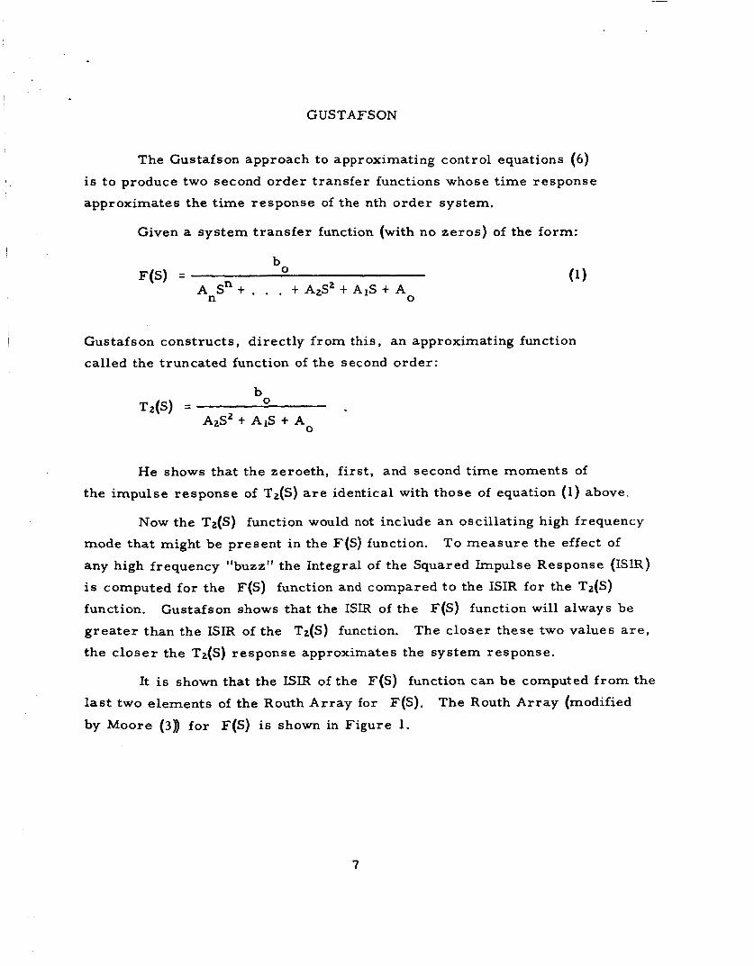
The Gustafson approach t o approximating control equations ( 6 )

is to produce two second order transfer functions whose t ime response

approximates the t ime response of the nth order system.

Given a system transfer function (with no zeros) of the form:

0 b

F(S) = A Sn t . . . t AzS't AIS t A

n 0

Gustafson constructs, directly from this, an approximating function

called the truncated function of the second order:

He shows that the zeroeth, f i rs t , and second time moments of

the impulse response of Tz(S) a r e identical with those of equation (1) above.

Now the Tz(S) function would not include an oscillating high frequency

mode that might be present in the F(S) function.

any high frequency "buzz" the Integral of the Squared Impulse Response (ISIR)

is computed for the F(S) function and compared to the ISIR for the Tz(S)

function. Gustafson shows that the ISIR of the F(S) function will always be

grea te r than the ISIR of the Tz(S) function. The closer these two values are,

the c loser the Tz(S) response approximates the system response.

To measu re the effect of

It is shown that the ISIR of the F(S) function can be computed f rom the

The Routh Array (modified last two elements of the Routh Ar ray for F(S).

by Moore (3)) fo r F(S) is shown in Figure 1 .

7

..... Az n- 2 *n- 3 A 0

A

Another approximating function called the associated function of the

second order i s constructed.

b 0

Az(s) = Rn-2SZ t R n- 1 S t A 0

Then the ISIR of the F(S) function is identical with that of the

Az(S) function. So computing the ISIR's f rom the Routh Array

b2 1 0

2 R n - l o

ISIR F(S) = ISIR Az(S) = - A

8

b2 1 0 2 and: ISIR Tz(S) = -

&Ao

then defining the energy ratio:

A1

n- 1 - ISIR Fz(S) - - El = ‘m R

This ra t io indicates how closely Tz(S) approximates F(S).

The Az(S) function is shown to have zeroeth, f i r s t , and second

frequency moments of its spectral energy distribution identical to the

corresponding moments of the F(S) function. Also the natural frequency

of the Az(S) approximation is shown to be equal to the W F(S) function.

of the rms

Gustafson then shows the following step response properties of

the T2(S) and Az(S) approximating functions.

T& - - - The s tep response of T&) has about the same mean time

delay as the sys tem response (resulting f rom identical

first t ime moments) and is generally a lower bound on

overshoot.

A&)-- The s tep response of A&) has about the same r i s e t ime

as the sys tem response (resulting f rom identical Wrms)

and is generally an upper bound on overshoot.

Thus the system response is seen to be approximated by two known

second order responses. The accuracy of the approximations A2(S) and

T2(S) can be compvted o r fixed by the designer using the El ratio.

Gustafson found that a tolerance of 1.4 to 1. 6 for El yields good resul ts .

9

1. I

2.

3.

4.

5.

6.

REFERENCES

Olderburger, R . , "Algebraic Approach to Design of Automatic

Controls, I' ASME Transactions, February, 1953, pp. 433-443.

Moore, J. W. and R. Oldenburger, "Rapid Methods for the Solution

of Automatic Control Equations, IEEE Transactions (Applications

and Industry), vol. 68, September 1963, pp. 286-295.

Moore, J . W. , "Rapid Algebraic Techniques f o r Solving Automatic

Control Equations, I ' Ph. D. Thesis, Purdue University , Lafayette,

Indiania, June 1962.

Krishnamurthy, E. V. , "Solving an Algebraic Equation by

Determining High Powers of an Associated Matrix Using the Cayley-

Hamilton Theorem, ' I The Quarterly Journal of Mechanics and

Applied Mathematics! vol. 13, November 1960.

Wilkinson, J . H. , The Algebraic Eigenvalue Problem, Oxford

University P r e s s , Amen House, London, 1965, pp. 579-581.

Gustafson, R. D . , "A Paper and Pencil Control System Design

Technique, I' Prepr in ts of Papers - - the 1965 Joint Automatic

Control Conference, June 1965, pp. 301-310.

.. .

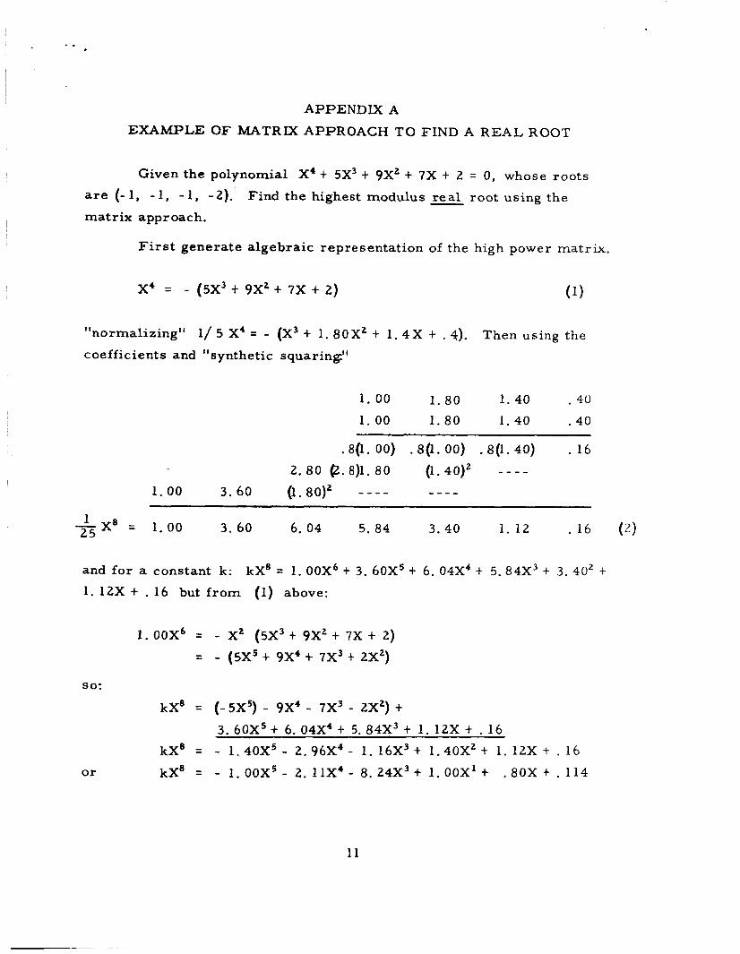
APPENDIX A

EXAMPLE OF MATRIX APPROACH TO FIND A REAL ROOT

Given the polynomial X't 5X3 + 9X2 t 7X t 2 = 0, whose roots

a r e (- 1, - 1, - 1, -2) .

matrix approach.

Find the highest modulus real root using the -

First generate algebraic representation of the high power matrix.

(1) x' = - (5x3 t 9X2+ 7 x t 2)

I 1 normalizing"

coefficients and "synthetic squaring:"

I/ 5 X' = - (X3 + 1. 80X2 t 1 . 4 X t . 4). Then using the

1. 00 1. 80 1. 40 . 4 0

1. 00 1. 80 1. 40 . 4 0

.@. 00) .8(1. OC) - 8 0 . 40) . 16

2. 8 0 @. 8)l. 80 (1.40)2 - - - - 1.00 3 . 60 (1.80)' - - - - - - - -

1 -x8 25 = 1.00 3. 60 6. 04 5. 84 3, 40 1. 12 . 16 (a)

and for a constant k:

1. 12X + . 16 but f rom (1) above:

kX8 = I . OOX't 3. 60X5 t 6. 04X4 t 5. 84X3 t 3.40' f

1. OOX' = - X2 (5x3 t 9x2 t 7 x + 2)

- (5x5 t 9x4 t 7x3 t 2x2) =

so:

kX8 = (-5X5) - 9X' - 7x3 - 2x2) + 3. 60X5 t 6. 04X4 t 5. 84X3 t 1.12X t . 16

kX8 = - 1. 40X5 - 2. 96X' - 1. 16X3 t 1.40X2 + 1, 12X t . 16

or kX8 = - 1. OOX5 - 2. l lX* - 8. 24X3 t 1. OOX't .80X t . 114

11

then again f rom ( I ) above we see that:

-1. 00x5 = x(sx3 + 9x2 t 7 x t 2).

And the process continues- - But an algorithm can be used to do these succeFsive substitutions more

efficiently. Going back t o line (2).

XB =

substituting

subtracting

normalizing

substituting

subtracting

normalizing

substituting

subtracting

normalizing

squaring

k4X l6

substituting

subtracting

normalizing

sub s t ituting

subt r acting

normalizing

substituting

subtracting

1. 00 3. 60 6. 04 5. 84 3 .40 1. 12 . 16

k - 5 . 0 0 -9 .00 -7 .00 -2 .00 -1 .40 -2 .96 -1. 16 t l . 4 0

-1 .00 -2 .11 - . 8 2 9 t l . 0 0 t , 8 0 t .114

t 5 . 0 0 t 9 . 0 0 t 7 . 0 0 t 2 . 0 0

2.89 t8 . 171 t8 . 00 t 1 . 8 0

1.00 t 2 . 8 3 t 2 . 7 7 t .969 t . 0394

k - 5 . 0 0 -9 .00 -7 .00 -2.000

-2.17 -6 .23 -6. 031 - 1,9606

k3X8 = 1.00 t 2 . 8 7 t 2 . 7 8 t . 9 0 4

1. 00 t 2 . 8 7 t 2 . 7 8 + . 9 0 4

1.81 +5.19 + 5 . 0 3 t . 8 1 7

5.56 t 1 5 . 9 6 4-7.73 - - - - _ _ - _ 1. 00 5.74 8 . 2 4 - - - - -

1.00 t 5 . 7 4 t 1 3 . 8 0 4-17.77 t 1 2 . 9 2 t 5 . 0 3 -t -817 N - 5 . 0 0 - 9 . 0 0 - 7 .00 - 2 .00

. 7 4 t 4 .80 t 1 0 . 7 7 t 1 0 . 9 2

1. 00 t 6 .49 t14 . 55 t 1 4 . 7 6 t 6 . 8 0 t 1 . 104

x- 5.00 - 9 .00 - 7 .00 -2 .00

1.49 t 5. 55 + 7 .76 t 4 . 8 0

1.00 3 .73 5 .21 3.22 . 7 4 1

- 5.00 - 9 . 0 0 -7 .00 - 2 . 0 0

- 1.27 - 3.79 -3 .78 -1 .26

1 . 0 0 2. 98 2.98 . 9 9 2 normalizing k k 1 6 =

12

Now assuming that sixteen "iterations" a r e enough we will find

the eigenvalue.

algebraic expression for the high power (16) matrix.

The "eigenvector" is found f rom coefficients of the

2.98 -9 + 2.98 6. 02 1. 00 -5 -I- 2.98 2.02

eigenvector

then removing the constant.

Eigenvalue (root) = - 2. 02 1. 00

The correctness of the eigenvalue can be checked by comparing the

multiplied vector with the product vector to see i f they a r e equal.

the 70 of difference in the two vectors is approximately the 70 of e r r o r

in the eigenvalue.

can be used.

If not,

If the e r r o r is too large, a higher power matr ix expression

The next step in this case would be the 32nd power.

13

DISTRIBUTION LIST

Copy No.

1 - 10

11

12 - 15

16

17 - 18

19 - 23

Office of Grants and Research Contracts Code SC National Aeronautics and Space Administration Washington 25, D, C.

A. R. Kuhlthau

J . W. Moore

J. J . Kauzlarich

Alderman Library

RLES F i l e s