کیناکم یسدنهم شزومآ...

http://www.Drshokuhi.com

سایت آموزش مهندسی مکانیک

426

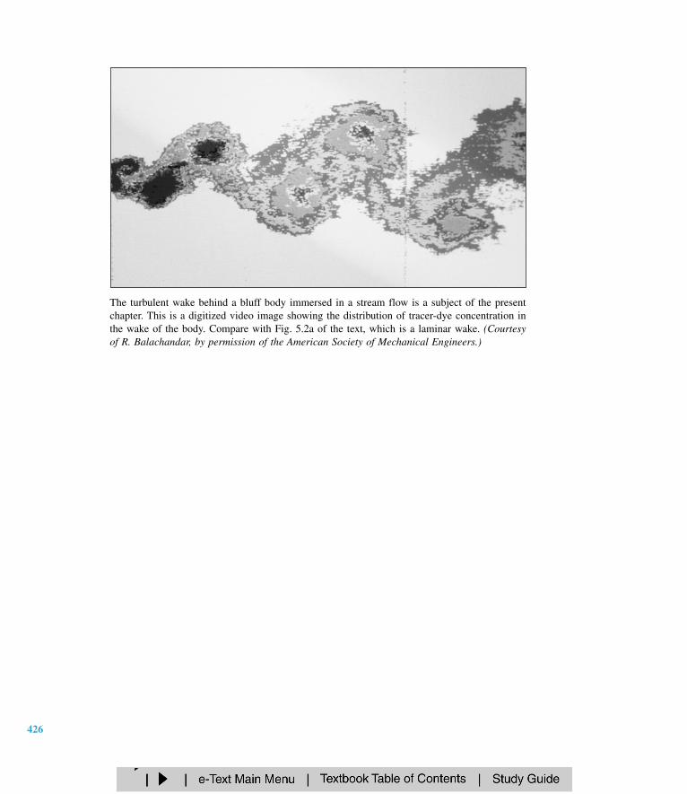
The turbulent wake behind a bluff body immersed in a stream flow is a subject of the presentchapter. This is a digitized video image showing the distribution of tracer-dye concentration inthe wake of the body. Compare with Fig. 5.2a of the text, which is a laminar wake. (Courtesyof R. Balachandar, by permission of the American Society of Mechanical Engineers.)

7.1 Reynolds-Numberand Geometry Effects

Motivation. This chapter is devoted to “external” flows around bodies immersed in afluid stream. Such a flow will have viscous (shear and no-slip) effects near the bodysurfaces and in its wake, but will typically be nearly inviscid far from the body. Theseare unconfined boundary-layer flows.

Chapter 6 considered “internal” flows confined by the walls of a duct. In that casethe viscous boundary layers grow from the sidewalls, meet downstream, and fill theentire duct. Viscous shear is the dominant effect. For example, the Moody chart of Fig.6.13 is essentially a correlation of wall shear stress for long ducts of constant crosssection.

External flows are unconfined, free to expand no matter how thick the viscous lay-ers grow. Although boundary-layer theory (Sec. 7.3) is helpful in understanding exter-nal flows, complex body geometries usually require experimental data on the forcesand moments caused by the flow. Such immersed-body flows are commonly encoun-tered in engineering studies: aerodynamics (airplanes, rockets, projectiles), hydrody-namics (ships, submarines, torpedos), transportation (automobiles, trucks, cycles), windengineering (buildings, bridges, water towers, wind turbines), and ocean engineering(buoys, breakwaters, pilings, cables, moored instruments). This chapter provides dataand analysis to assist in such studies.

The technique of boundary-layer (BL) analysis can be used to compute viscous effectsnear solid walls and to “patch” these onto the outer inviscid motion. This patching ismore successful as the body Reynolds number becomes larger, as shown in Fig. 7.1.

In Fig. 7.1 a uniform stream U moves parallel to a sharp flat plate of length L. Ifthe Reynolds number UL/ is low (Fig. 7.1a), the viscous region is very broad and ex-tends far ahead and to the sides of the plate. The plate retards the oncoming streamgreatly, and small changes in flow parameters cause large changes in the pressure dis-tribution along the plate. Thus, although in principle it should be possible to patch the

427

Chapter 7Flow Past

Immersed Bodies

Fig. 7.1 Comparison of flow past asharp flat plate at low and highReynolds numbers: (a) laminar,low-Re flow; (b) high-Re flow.

viscous and inviscid layers in a mathematical analysis, their interaction is strong andnonlinear [1 to 3]. There is no existing simple theory for external-flow analysis atReynolds numbers from 1 to about 1000. Such thick-shear-layer flows are typicallystudied by experiment or by numerical modeling of the flow field on a digital com-puter [4].

A high-Reynolds-number flow (Fig. 7.1b) is much more amenable to boundary-layerpatching, as first pointed out by Prandtl in 1904. The viscous layers, either laminar orturbulent, are very thin, thinner even than the drawing shows. We define the boundary-layer thickness as the locus of points where the velocity u parallel to the plate reaches99 percent of the external velocity U. As we shall see in Sec. 7.4, the accepted for-mulas for flat-plate flow are

x

laminar (7.1a)

turbulent (7.1b)0.16Rex

1/7

5.0Rex

1/2

428 Chapter 7 Flow Past Immersed Bodies

Large viscousdisplacement

effect

ReL = 10

U

x

L

Viscousregion

Inviscid regionU

U

u < U

u = 0.99Uδ ≈ L

x

U

U

u < UViscous

Inviscid region

δ L

Laminar BL

Turbulent BL

Smalldisplacement

effect

ReL = 107

U

(a)

(b)

Fig. 7.2 Illustration of the stronginteraction between viscous and in-viscid regions in the rear of blunt-body flow: (a) idealized and defi-nitely false picture of blunt-bodyflow; (b) actual picture of blunt-body flow.

where Rex Ux/ is called the local Reynolds number of the flow along the plate sur-face. The turbulent-flow formula applies for Rex greater than approximately 106.

Some computed values from Eq. (7.1) are

Rex 104 105 106 107 108

(/x)lam 0.050 0.016 0.005

(/x)turb 0.022 0.016 0.011

The blanks indicate that the formula is not applicable. In all cases these boundary lay-ers are so thin that their displacement effect on the outer inviscid layer is negligible.Thus the pressure distribution along the plate can be computed from inviscid theory asif the boundary layer were not even there. This external pressure field then “drives”the boundary-layer flow, acting as a forcing function in the momentum equation alongthe surface. We shall explain this boundary-layer theory in Secs. 7.4 and 7.5.

For slender bodies, such as plates and airfoils parallel to the oncoming stream, weconclude that this assumption of negligible interaction between the boundary layer andthe outer pressure distribution is an excellent approximation.

For a blunt-body flow, however, even at very high Reynolds numbers, there is a dis-crepancy in the viscous-inviscid patching concept. Figure 7.2 shows two sketches offlow past a two- or three-dimensional blunt body. In the idealized sketch (7.2a), thereis a thin film of boundary layer about the body and a narrow sheet of viscous wake inthe rear. The patching theory would be glorious for this picture, but it is false. In the

7.1 Reynolds-Number and Geometry Effects 429

(a)

(b)

Thin frontboundary layer

Beautifully behavedbut mythically thin

boundary layerand wake

Outer stream grosslyperturbed by broad flow

separation and wake

Red = 10

5

Red = 10

5

actual flow (Fig. 7.2b), the boundary layer is thin on the front, or windward, side ofthe body, where the pressure decreases along the surface (favorable pressure gradient).But in the rear the boundary layer encounters increasing pressure (adverse pressuregradient) and breaks off, or separates, into a broad, pulsating wake. (See Fig. 5.2a fora photograph of a specific example.) The mainstream is deflected by this wake, so thatthe external flow is quite different from the prediction from inviscid theory with theaddition of a thin boundary layer.

The theory of strong interaction between blunt-body viscous and inviscid layers isnot well developed. Flows like that of Fig. 7.2b are normally studied experimentally.Reference 5 is an example of efforts to improve the theory of separated-boundary-layerflows. Reference 6 is a textbook devoted to separated flow.

EXAMPLE 7.1

A long, thin flat plate is placed parallel to a 20-ft/s stream of water at 20°C. At what distance xfrom the leading edge will the boundary-layer thickness be 1 in?

Solution

Since we do not know the Reynolds number, we must guess which of Eqs. (7.1) applies. FromTable 1.4 for water, 1.09 105 ft2/s; hence

U

1.09

201f0t

/s5 ft2/s

1.84 106 ft1

With 1 in 112 ft, try Eq. (7.1a):

Laminar flow:

x

(Ux/5)1/2

or x 2(

5U2/v)

511 ft

Now we can test the Reynolds number to see whether the formula applied:

Rex U

x

1(.2009

f

t/s1)0(5

151ftf2t)/s

9.4 108

This is impossible since the maximum Rex for laminar flow past a flat plate is 3 106. So wetry again with Eq. (7.1b):

Turbulent flow:

x

(U0x./1

6)1/7

or x 7/6

7/6

(4.09)7/6 5.17 ft Ans.

Test Rex 1(.2009

f

t/s1)(05

.157ftf2t/)s

9.5 106

This is a perfectly proper turbulent-flow condition; hence we have found the correct position xon our second try.

(112 ft)(1.84 106 ft1)1/7

0.16

(U/v)1/ 7

0.16

(112 ft)2(1.84 106 ft1)

25


7.2 Momentum-IntegralEstimates

Kármán’s Analysis of the Flat Plate

Fig. 7.3 Growth of a boundarylayer on a flat plate.

When we derived the momentum-integral relation, Eq. (3.37), and applied it to a flat-plate boundary layer in Example 3.11, we promised to consider it further in Chap. 7.Well, here we are! Let us review the problem, using Fig. 7.3.

A shear layer of unknown thickness grows along the sharp flat plate in Fig. 7.3. Theno-slip wall condition retards the flow, making it into a rounded profile u(y), whichmerges into the external velocity U constant at a “thickness” y (x). By utilizingthe control volume of Fig. 3.11, we found (without making any assumptions about lam-inar versus turbulent flow) in Example 3.11 that the drag force on the plate is given bythe following momentum integral across the exit plane

D(x) b (x)

0u(U u) dy (7.2)

where b is the plate width into the paper and the integration is carried out along a ver-tical plane x constant. You should review the momentum-integral relation (3.37) andits use in Example 3.11.

Equation (7.2) was derived in 1921 by Kármán [7], who wrote it in the convenient formof the momentum thickness

D(x) bU2

0Uu

1 Uu

dy (7.3)

Momentum thickness is thus a measure of total plate drag. Kármán then noted that thedrag also equals the integrated wall shear stress along the plate

D(x) b x

0w(x) dx

or ddDx bw (7.4)

Meanwhile, the derivative of Eq. (7.3), with U constant, is

ddDx bU2

dd

x

By comparing this with Eq. (7.4) Kármán arrived at what is now called the momentum-integral relation for flat-plate boundary-layer flow

7.2 Momentum-Integral Estimates 431

x

y

U

x = 0

p = pa

U

w (x)

x = L

u (x, y)

U

(x)δ

τ

w U2 dd

x (7.5)

It is valid for either laminar or turbulent flat-plate flow.To get a numerical result for laminar flow, Kármán assumed that the velocity pro-

files had an approximately parabolic shape

u(x, y) U2

y

y2

2 0 y (x) (7.6)

which makes it possible to estimate both momentum thickness and wall shear

0 2

y

y2

21 2

y

y2

2 dy 125

(7.7)

w

uyy0

2

U

By substituting (7.7) into (7.5) and rearranging we obtain

d 15 U

dx (7.8)

where /. We can integrate from 0 to x, assuming that 0 at x 0, the lead-ing edge

12

2 15

Ux

or

x 5.5

U

x

1/2

(7.9)

This is the desired thickness estimate. It is all approximate, of course, part of Kár-mán’s momentum-integral theory [7], but it is startlingly accurate, being only 10 per-cent higher than the known exact solution for laminar flat-plate flow, which we gaveas Eq. (7.1a).

By combining Eqs. (7.9) and (7.7) we also obtain a shear-stress estimate along theplate

cf

2Uw

2 1/2

(7.10)

Again this estimate, in spite of the crudeness of the profile assumption (7.6) is only 10percent higher than the known exact laminar-plate-flow solution cf 0.664/Rex

1/2,treated in Sec. 7.4. The dimensionless quantity cf, called the skin-friction coefficient,is analogous to the friction factor f in ducts.

A boundary layer can be judged as “thin” if, say, the ratio /x is less than about 0.1.This occurs at /x 0.1 5.0/Rex

1/2 or at Rex 2500. For Rex less than 2500 we canestimate that boundary-layer theory fails because the thick layer has a significant effecton the outer inviscid flow. The upper limit on Rex for laminar flow is about 3 106,where measurements on a smooth flat plate [8] show that the flow undergoes transitionto a turbulent boundary layer. From 3 106 upward the turbulent Reynolds number maybe arbitrarily large, and a practical limit at present is 5 109 for oil supertankers.

0.73Rex

1/2

185

Rex

5.5Rex

1/2


Displacement Thickness

Fig. 7.4 Displacement effect of aboundary layer.

Another interesting effect of a boundary layer is its small but finite displacement ofthe outer streamlines. As shown in Fig. 7.4, outer streamlines must deflect outward adistance *(x) to satisfy conservation of mass between the inlet and outlet

h

0Ub dy

0ub dy h * (7.11)

The quantity * is called the displacement thickness of the boundary layer. To relate itto u(y), cancel and b from Eq. (7.11), evaluate the left integral, and slyly add andsubtract U from the right integrand:

Uh

0(U u U) dy U(h *)

0(u U) dy

or *

0 1 Uu

dy (7.12)

Thus the ratio of */ varies only with the dimensionless velocity-profile shape u/U.Introducing our profile approximation (7.6) into (7.12), we obtain by integration the

approximate result

* 13

x* (7.13)

These estimates are only 6 percent away from the exact solutions for laminar flat-plateflow given in Sec. 7.4: * 0.344 1.721x/Rex

1/2. Since * is much smaller than xfor large Rex and the outer streamline slope V/U is proportional to *, we concludethat the velocity normal to the wall is much smaller than the velocity parallel to thewall. This is a key assumption in boundary-layer theory (Sec. 7.3).

We also conclude from the success of these simple parabolic estimates that Kár-mán’s momentum-integral theory is effective and useful. Many details of this theoryare given in Refs. 1 to 3.

EXAMPLE 7.2

Are low-speed, small-scale air and water boundary layers really thin? Consider flow at U 1ft/s past a flat plate 1 ft long. Compute the boundary-layer thickness at the trailing edge for (a)air and (b) water at 20°C.

1.83Rex

1/2

7.2 Momentum-Integral Estimates 433

yU U

Simulatedeffect

0

y = h

x

Outer streamline

y = h +

U

uδ *

h

h

δ *

Part (a)

Part (b)

7.3 The Boundary-LayerEquations

Solution

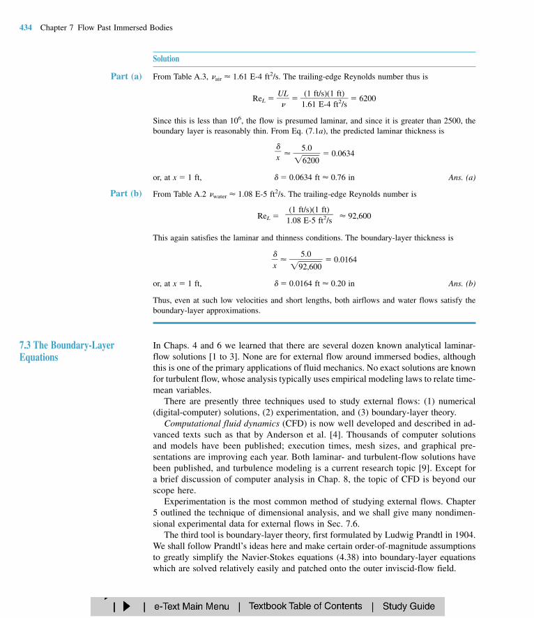
From Table A.3, air 1.61 E-4 ft2/s. The trailing-edge Reynolds number thus is

ReL U

L

1(.161

ftE/s

-)4(1

ftf2t/)s

6200

Since this is less than 106, the flow is presumed laminar, and since it is greater than 2500, theboundary layer is reasonably thin. From Eq. (7.1a), the predicted laminar thickness is

0.0634

or, at x 1 ft, 0.0634 ft 0.76 in Ans. (a)

From Table A.2 water 1.08 E-5 ft2/s. The trailing-edge Reynolds number is

ReL 92,600

This again satisfies the laminar and thinness conditions. The boundary-layer thickness is

x 0.0164

or, at x 1 ft, 0.0164 ft 0.20 in Ans. (b)

Thus, even at such low velocities and short lengths, both airflows and water flows satisfy theboundary-layer approximations.

In Chaps. 4 and 6 we learned that there are several dozen known analytical laminar-flow solutions [1 to 3]. None are for external flow around immersed bodies, althoughthis is one of the primary applications of fluid mechanics. No exact solutions are knownfor turbulent flow, whose analysis typically uses empirical modeling laws to relate time-mean variables.

There are presently three techniques used to study external flows: (1) numerical(digital-computer) solutions, (2) experimentation, and (3) boundary-layer theory.

Computational fluid dynamics (CFD) is now well developed and described in ad-vanced texts such as that by Anderson et al. [4]. Thousands of computer solutionsand models have been published; execution times, mesh sizes, and graphical pre-sentations are improving each year. Both laminar- and turbulent-flow solutions havebeen published, and turbulence modeling is a current research topic [9]. Except fora brief discussion of computer analysis in Chap. 8, the topic of CFD is beyond ourscope here.

Experimentation is the most common method of studying external flows. Chapter5 outlined the technique of dimensional analysis, and we shall give many nondimen-sional experimental data for external flows in Sec. 7.6.

The third tool is boundary-layer theory, first formulated by Ludwig Prandtl in 1904.We shall follow Prandtl’s ideas here and make certain order-of-magnitude assumptionsto greatly simplify the Navier-Stokes equations (4.38) into boundary-layer equationswhich are solved relatively easily and patched onto the outer inviscid-flow field.

5.092,600

(1 ft/s)(1 ft)1.08 E-5 ft2/s

5.06200

x


Derivation for Two-DimensionalFlow

One of the great achievements of boundary-layer theory is its ability to predict theflow separation illustrated in Fig. 7.2b. Before 1904 no one realized that such thin shearlayers could cause such a gross effect as flow separation. Unfortunately, even today the-ory cannot accurately predict the behavior of the separated-flow region and its interac-tion with the outer layer. This is the weakness of boundary-layer theory, which we hopewill be overcome by intensive research into the dynamics of separated flows [6].

We consider only steady two-dimensional incompressible viscous flow with the x di-rection along the wall and y normal to the wall, as in Fig. 7.3.1 We neglect gravity,which is important only in boundary layers where fluid buoyancy is dominant [2, sec.4.13]. From Chap. 4, the complete equations of motion consist of continuity and thex- and y-momentum relations

ux

y 0 (7.14a)

u

ux

uy

px

2

xu2

2

yu2 (7.14b)

u

x

y

py

2

x2

2

y2 (7.14c)

These should be solved for u, , and p subject to typical no-slip, inlet, and exit bound-ary conditions, but in fact they are too difficult to handle for most external flows.

In 1904 Prandtl correctly deduced that a shear layer must be very thin if the Reynoldsnumber is large, so that the following approximations apply:

Velocities: u (7.15a)

Rates of change:

ux

uy

x

y (7.15b)

Our discussion of displacement thickness in the previous section was intended to jus-tify these assumptions.

Applying these approximations to Eq. (7.14c) results in a powerful simplification

py 0 or p p(x) only (7.16)

In other words, the y-momentum equation can be neglected entirely, and the pressurevaries only along the boundary layer, not through it. The pressure-gradient term in Eq.(7.14b) is assumed to be known in advance from Bernoulli’s equation applied to theouter inviscid flow

px

ddpx U

ddUx (7.17)

7.3 The Boundary-Layer Equations 435

1For a curved wall, x can represent the arc length along the wall and y can be everywhere normal to xwith negligible change in the boundary-layer equations as long as the radius of curvature of the wall islarge compared with the boundary-layer thickness [1 to 3].

7.4 The Flat-Plate BoundaryLayer

Presumably we have already made the inviscid analysis and know the distribution ofU(x) along the wall (Chap. 8).

Meanwhile, one term in Eq. (7.14b) is negligible due to Eqs. (7.15)

2

xu2

2

yu2 (7.18)

However, neither term in the continuity relation (7.14a) can be neglected—anotherwarning that continuity is always a vital part of any fluid-flow analysis.

The net result is that the three full equations of motion (7.14) are reduced to Prandtl’stwo boundary-layer equations

Continuity:

ux

y 0 (7.19a)

Momentum along wall: u

ux

uy U

ddUx

1

y (7.19b)

where

uy laminar flow

uy u turbulent flow

These are to be solved for u(x, y) and (x, y), with U(x) assumed to be a known func-tion from the outer inviscid-flow analysis. There are two boundary conditions on u andone on :

At y 0 (wall): u 0 (no slip) (7.20a)

At y (x) (outer stream): u U(x) (patching) (7.20b)

Unlike the Navier-Stokes equations (7.14), which are mathematically elliptic and mustbe solved simultaneously over the entire flow field, the boundary-layer equations (7.19)are mathematically parabolic and are solved by beginning at the leading edge andmarching downstream as far as you like, stopping at the separation point or earlier ifyou prefer.2

The boundary-layer equations have been solved for scores of interesting cases ofinternal and external flow for both laminar and turbulent flow, utilizing the invisciddistribution U(x) appropriate to each flow. Full details of boundary-layer theory andresults and comparison with experiment are given in Refs. 1 to 3. Here we shall con-fine ourselves primarily to flat-plate solutions (Sec. 7.4).

The classic and most often used solution of boundary-layer theory is for flat-plate flow,as in Fig. 7.3, which can represent either laminar or turbulent flow.


2For further mathematical details, see Ref. 2, sec. 2.8.

Laminar Flow For laminar flow past the plate, the boundary-layer equations (7.19) can be solved ex-actly for u and , assuming that the free-stream velocity U is constant (dU/dx 0).The solution was given by Prandtl’s student Blasius, in his 1908 dissertation from Göt-tingen. With an ingenious coordinate transformation, Blasius showed that the dimen-sionless velocity profile u/U is a function only of the single composite dimensionlessvariable (y)[U/(x)]1/2:

Uu

f() yvUx

1/2

(7.21)

where the prime denotes differentiation with respect to . Substitution of (7.21) intothe boundary-layer equations (7.19) reduces the problem, after much algebra, to a sin-gle third-order nonlinear ordinary differential equation for f

f 12

ff 0 (7.22)

The boundary conditions (7.20) become

At y 0: f(0) f(0) 0 (7.23a)

As y → : f() → 1.0 (7.23b)

This is the Blasius equation, for which accurate solutions have been obtained only bynumerical integration. Some tabulated values of the velocity-profile shape f() u/Uare given in Table 7.1.

Since u/U approaches 1.0 only as y → , it is customary to select the boundary-layer thickness as that point where u/U 0.99. From the table, this occurs at 5.0:

99%

Ux

1/2

5.0

or

x Blasius (1908) (7.24)

5.0Rex

1/2

7.4 The Flat-Plate Boundary Layer 437

y[U/(x)]1/2 u/U y[U/(x)]1/2 u/U

0.0 0.0 2.8 0.811520.2 0.06641 3.0 0.846050.4 0.13277 3.2 0.876090.6 0.19894 3.4 0.901770.8 0.26471 3.6 0.923331.0 0.32979 3.8 0.941121.2 0.39378 4.0 0.955521.4 0.45627 4.2 0.966961.6 0.51676 4.4 0.975871.8 0.57477 4.6 0.982692.0 0.62977 4.8 0.987792.2 0.68132 5.0 0.991552.4 0.72899 1.000002.6 0.77246

Table 7.1 The Blasius VelocityProfile [1 to 3]

With the profile known, Blasius, of course, could also compute the wall shear and dis-placement thickness

cf

x* (7.25)

Notice how close these are to our integral estimates, Eqs. (7.9), (7.10), and (7.13).When cf is converted to dimensional form, we have

w(x) 0.3321

x

/

1

2

/ 2

1/2U1.5

The wall shear drops off with x1/2 because of boundary-layer growth and varies as ve-locity to the 1.5 power. This is in contrast to laminar pipe flow, where w U and isindependent of x.

If w(x) is substituted into Eq. (7.4), we compute the total drag force

D(x) b x

0w(x) dx 0.664b1/2 1/2U1.5x1/2 (7.26)

The drag increases only as the square root of the plate length. The nondimensionaldrag coefficient is defined as

CD

2UD

2(bLL)

2cf (L) (7.27)

Thus, for laminar plate flow, CD equals twice the value of the skin-friction coefficientat the trailing edge. This is the drag on one side of the plate.

Kármán pointed out that the drag could also be computed from the momentum re-lation (7.2). In dimensionless form, Eq. (7.2) becomes

CD L2

0Uu

1 Uu

dy (7.28)

This can be rewritten in terms of the momentum thickness at the trailing edge

CD 2

L(L) (7.29)

Computation of from the profile u/U or from CD gives

x laminar flat plate (7.30)

Since is so ill defined, the momentum thickness, being definite, is often used to cor-relate data taken for a variety of boundary layers under differing conditions. The ratioof displacement to momentum thickness, called the dimensionless-profile shape fac-tor, is also useful in integral theories. For laminar flat-plate flow

H 10..762614

2.59 (7.31)

A large shape factor then implies that boundary-layer separation is about to occur.

*

0.664Rex

1/2

1.328ReL

1/2

1.721Rex

1/2

0.664Rex

1/2


Fig. 7.5 Comparison of dimension-less laminar and turbulent flat-platevelocity profiles.

Transition to Turbulence

If we plot the Blasius velocity profile from Table 7.1 in the form of u/U versus y/,we can see why the simple integral-theory guess, Eq. (7.6), was such a great success.This is done in Fig. 7.5. The simple parabolic approximation is not far from the trueBlasius profile; hence its momentum thickness is within 10 percent of the true value.Also shown in Fig. 7.5 are three typical turbulent flat-plate velocity profiles. Notice howstrikingly different in shape they are from the laminar profiles. Instead of decreasingmonotonically to zero, the turbulent profiles are very flat and then drop off sharply atthe wall. As you might guess, they follow the logarithmic-law shape and thus can beanalyzed by momentum-integral theory if this shape is properly represented.

The laminar flat-plate boundary layer eventually becomes turbulent, but there is nounique value for this change to occur. With care in polishing the wall and keeping thefree stream quiet, one can delay the transition Reynolds number to Rex,tr 3 E6 [8].However, for typical commercial surfaces and gusty free streams, a more realistic valueis Rex,tr 5 E5.

EXAMPLE 7.3

A sharp flat plate with L 1 m and b 3 m is immersed parallel to a stream of velocity 2 m/s.Find the drag on one side of the plate, and at the trailing edge find the thicknesses , *, and for (a) air, 1.23 kg/m3 and 1.46 105 m2/s, and (b) water, 1000 kg/m3 and 1.02 106 m2/s.


1.0

0.8

0.6

0.4

0.2

00.2 0.4 0.6 0.8 1.0

uU

y

δ

Turbulent

10

5 = Rex10

6

10

7

Seventhroot profile,Eq. (7.39)

Exact Blasius profilefor all laminar Rex

( Table 7.1)

Parabolicapproximation,

Eq. ( 7.6)

Part (b)

Part (a)

Solution

The airflow Reynolds number is

V

L

1(.24.60

m/1s0)(

15.0

mm2/)s

137,000

Since this is less than 3 106, we assume that the boundary layer is laminar. From Eq. (7.27),the drag coefficient is

CD (13

17.,302080)1/2 0.00359

Thus the drag on one side in the airflow is

D CD12

U2bL 0.00359(12

)(1.23)(2.0)2(3.0)(1.0) 0.0265 N Ans. (a)

The boundary-layer thickness at the end of the plate is

L

(137

5,0.000)1/2 0.0135

or 0.0135(1.0) 0.0135 m 13.5 mm Ans. (a)

We find the other two thicknesses simply by ratios:

* 1.57.201

4.65 mm 2

.5*9

1.79 mm Ans. (a)

Notice that no conversion factors are needed with SI units.

The water Reynolds number is

ReL 1.0

22.0

(1.100)6 1.96 106

This is rather close to the critical value of 3 106, so that a rough surface or noisy free streammight trigger transition to turbulence; but let us assume that the flow is laminar. The water dragcoefficient is

CD (1.96

1

.321806)1/2 0.000949

and D 0.000949(12

)(1000)(2.0)2(3.0)(1.0) 5.70 N Ans. (b)

The drag is 215 times more for water in spite of the higher Reynolds number and lower dragcoefficient because water is 57 times more viscous and 813 times denser than air. From Eq.(7.26), in laminar flow, it should have (57)1/2(813)1/2 7.53(28.5) 215 times more drag.

The boundary-layer thickness is given by

L

(1.96

5.0106)1/2 0.00357

or 0.00357(1000 mm) 3.57 mm Ans. (b)

By scaling down we have

5.0ReL

1/2


Turbulent Flow

* 1.57.201

1.23 mm 2

.5*9

0.48 mm Ans. (b)

The water layer is 3.8 times thinner than the air layer, which reflects the square root of the 14.3ratio of air to water kinematic viscosity.

There is no exact theory for turbulent flat-plate flow, although there are many elegantcomputer solutions of the boundary-layer equations using various empirical models forthe turbulent eddy viscosity [9]. The most widely accepted result is simply an integalanalysis similar to our study of the laminar-profile approximation (7.6).

We begin with Eq. (7.5), which is valid for laminar or turbulent flow. We write ithere for convenient reference:

w(x) U2 dd

x (7.32)

From the definition of cf, Eq. (7.10), this can be rewritten as

cf 2 dd

x (7.33)

Now recall from Fig. 7.5 that the turbulent profiles are nowhere near parabolic. Goingback to Fig. 6.9, we see that flat-plate flow is very nearly logarithmic, with a slightouter wake and a thin viscous sublayer. Therefore, just as in turbulent pipe flow, weassume that the logarithmic law (6.21) holds all the way across the boundary layer

uu*

1 ln

yu

* B u*

w

1/2

(7.34)

with, as usual, 0.41 and B 5.0. At the outer edge of the boundary layer, y and u U, and Eq. (7.34) becomes

uU*

1 ln

u

* B (7.35)

But the definition of the skin-friction coefficient, Eq. (7.10), is such that the followingidentities hold:

uU*

c2

f

1/2

u

* Re

1/2

(7.36)

Therefore Eq. (7.35) is a skin-friction law for turbulent flat-plate flow

c2

f

1/2

2.44 ln Re 1/2

5.0 (7.37)

It is a complicated law, but we can at least solve for a few values and list them:

Re 104 105 106 107

cf 0.00493 0.00315 0.00217 0.00158

cf2

cf2


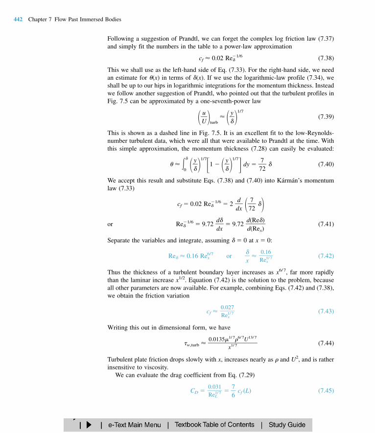
Following a suggestion of Prandtl, we can forget the complex log friction law (7.37)and simply fit the numbers in the table to a power-law approximation

cf 0.02 Re1/6 (7.38)

This we shall use as the left-hand side of Eq. (7.33). For the right-hand side, we needan estimate for (x) in terms of (x). If we use the logarithmic-law profile (7.34), weshall be up to our hips in logarithmic integrations for the momentum thickness. Insteadwe follow another suggestion of Prandtl, who pointed out that the turbulent profiles inFig. 7.5 can be approximated by a one-seventh-power law

Uu

turb

y

1/7

(7.39)

This is shown as a dashed line in Fig. 7.5. It is an excellent fit to the low-Reynolds-number turbulent data, which were all that were available to Prandtl at the time. Withthis simple approximation, the momentum thickness (7.28) can easily be evaluated:

0

y

1/7

1

y

1/7

dy 772 (7.40)

We accept this result and substitute Eqs. (7.38) and (7.40) into Kármán’s momentumlaw (7.33)

cf 0.02 Re1/6 2

ddx

772

or Re1/6 9.72

dd

x 9.72

dd((RR

ee

x))

(7.41)

Separate the variables and integrate, assuming 0 at x 0:

Re 0.16 Rex6/7 or

x (7.42)

Thus the thickness of a turbulent boundary layer increases as x6/ 7, far more rapidlythan the laminar increase x1/2. Equation (7.42) is the solution to the problem, becauseall other parameters are now available. For example, combining Eqs. (7.42) and (7.38),we obtain the friction variation

cf (7.43)

Writing this out in dimensional form, we have

w,turb (7.44)

Turbulent plate friction drops slowly with x, increases nearly as and U2, and is ratherinsensitive to viscosity.

We can evaluate the drag coefficient from Eq. (7.29)

CD 76

cf (L) (7.45)0.031ReL

1/ 7

0.0135 1/ 76/ 7U13/ 7

x1/ 7

0.027Rex

1/ 7

0.16Rex

1/ 7


Fig. 7.6 Drag coefficient of laminarand turbulent boundary layers onsmooth and rough flat plates. Thischart is the flat-plate analog of theMoody diagram of Fig. 6.13.

Then CD is only 16 percent greater than the trailing-edge skin friction [compare withEq. (7.27) for laminar flow].

The displacement thickness can be estimated from the one-seventh-power law andEq. (7.12):

*

0 1

y

1/ 7

dy 18

(7.46)

The turbulent flat-plate shape factor is approximately

H

* 1.3 (7.47)

These are the basic results of turbulent flat-plate theory.Figure 7.6 shows flat-plate drag coefficients for both laminar-and turbulent-flow

conditions. The smooth-wall relations (7.27) and (7.45) are shown, along with the ef-fect of wall roughness, which is quite strong. The proper roughness parameter here isx/ or L/, by analogy with the pipe parameter /d. In the fully rough regime, CD is in-dependent of the Reynolds number, so that the drag varies exactly as U2 and is inde-

18

772


0.014

0.012

0.010

0.008

0.006

0.004

010

5 10

8

ReL

Laminar:Eq. ( 7.27 )

Turbulentsmooth

Eq. ( 7.45 )

Transition

Eq. ( 7.49 )

200

500

1000

2000

10

4

2 × 10

4

2 × 10

5

0.002

10

6 10

7 10

9

CD

5 × 10

4

Lε = 300

10

6

Fully roughEq. ( 7.48b)

5000

Part (b)

Part (a)

pendent of . Reference 2 presents a theory of rough flat-plate flow, and Ref. 1 givesa curve fit for skin friction and drag in the fully rough regime:

cf 2.87 1.58 log x

2.5

(7.48a)

CD 1.89 1.62 log L

2.5

(7.48b)

Equation (7.48b) is plotted to the right of the dashed line in Fig. 7.6. The figure alsoshows the behavior of the drag coefficient in the transition region 5 105 ReL 8 107, where the laminar drag at the leading edge is an appreciable fraction of thetotal drag. Schlichting [1] suggests the following curve fits for these transition dragcurves depending upon the Reynolds number Retrans where transition begins:

CD

1R4e4

L

0 Retrans 5 105 (7.49a)

CD 8R7e0

L

0 Retrans 3 106 (7.49b)

EXAMPLE 7.4

A hydrofoil 1.2 ft long and 6 ft wide is placed in a water flow of 40 ft/s, with 1.99slugs/ft3 and 0.000011 ft2/s. (a) Estimate the boundary-layer thickness at the end of theplate. Estimate the friction drag for (b) turbulent smooth-wall flow from the leading edge,(c) laminar turbulent flow with Retrans 5 105, and (d) turbulent rough-wall flow with 0.0004 ft.

Solution

The Reynolds number is

ReL U

L

(04.000

f0t/0s)1(11.

f2t2

f/ts)

4.36 106

Thus the trailing-edge flow is certainly turbulent. The maximum boundary-layer thickness wouldoccur for turbulent flow starting at the leading edge. From Eq. (7.42),

(

LL)

(4.360

.11606)1/7 0.018

or 0.018(1.2 ft) 0.0216 ft Ans. (a)

This is 7.5 times thicker than a fully laminar boundary layer at the same Reynolds number.

For fully turbulent smooth-wall flow, the drag coefficient on one side of the plate is, from Eq.(7.45),

CD (4.36

0

.031106)1/7 0.00349

0.031ReL

1/ 7

0.031ReL

1/ 7


Part (c)

Part (d)

Then the drag on both sides of the foil is approximately

D 2CD(12

U2)bL 2(0.00349)(12

)(1.99)(40)2(6.0)(1.2) 80 lb Ans. (b)

With a laminar leading edge and Retrans 5 105, Eq. (7.49a) applies:

CD 0.00349 4.3

164

40106 0.00316

The drag can be recomputed for this lower drag coefficient:

D 2CD(12

U2)bL 72 lbf Ans. (c)

Finally, for the rough wall, we calculate

L

0.

10.0204

ftft

3000

From Fig. 7.6 at ReL 4.36 106, this condition is just inside the fully rough regime. Equa-tion (7.48b) applies:

CD (1.89 1.62 log 3000)2.5 0.00644

and the drag estimate is

D 2CD(12

U2)bL 148 lbf Ans. (d)

This small roughness nearly doubles the drag. It is probable that the total hydrofoil drag is stillanother factor of 2 larger because of trailing-edge flow-separation effects.

The flat-plate analysis of the previous section should give us a good feeling for the be-havior of both laminar and turbulent boundary layers, except for one important effect:flow separation. Prandtl showed that separation like that in Fig. 7.2b is caused by ex-cessive momentum loss near the wall in a boundary layer trying to move downstreamagainst increasing pressure, dp/dx 0, which is called an adverse pressure gradient.The opposite case of decreasing pressure, dp/dx 0, is called a favorable gradient,where flow separation can never occur. In a typical immersed-body flow, e.g., Fig. 7.2b,the favorable gradient is on the front of the body and the adverse gradient is in the rear,as discussed in detail in Chap. 8.

We can explain flow separation with a geometric argument about the second deriv-ative of velocity u at the wall. From the momentum equation (7.19b) at the wall, whereu 0, we obtain

ywall

2

yu2wall

U ddUx

ddpx

or

2

yu2wall

1

ddpx (7.50)

7.5 Boundary Layers with Pressure Gradient 445

3This section may be omitted without loss of continuity.

7.5 Boundary Layers withPressure Gradient3

Fig. 7.7 Effect of pressure gradienton boundary-layer profiles; PI point of inflection.

for either laminar or turbulent flow. Thus in an adverse gradient the second derivative ofvelocity is positive at the wall; yet it must be negative at the outer layer (y ) to mergesmoothly with the mainstream flow U(x). It follows that the second derivative must passthrough zero somewhere in between, at a point of inflection, and any boundary-layer profile in an adverse gradient must exhibit a characteristic S shape.

Figure 7.7 illustrates the general case. In a favorable gradient (Fig. 7.7a) the profile


U

u

PI

(a) Favorablegradient:

d Ud x

> 0

d p

d x< 0

No separation,PI inside wall

(b) Zerogradient:

d Ud x

= 0

d p

d x= 0

No separation,PI at wall

PIτ w = 0

(c) Weak adversegradient:

d Ud x

< 0

d p

d x> 0

No separation,PI in the flow

(d ) Critical adversegradient:

Zero slopeat the wall:

Separation

(e) Excessive adversegradient:

Backflowat the wall:

Separatedflow region

U

u

U

u

U

u

U

u

d p

d x> 0

PI

PI

Backflow

Fig. 7.8 Boundary-layer growth andseparation in a nozzle-diffuser con-figuration.

is very rounded, there is no point of inflection, there can be no separation, and lami-nar profiles of this type are very resistant to a transition to turbulence [1 to 3].

In a zero pressure gradient (Fig. 7.7b), e.g., flat-plate flow, the point of inflectionis at the wall itself. There can be no separation, and the flow will undergo transitionat Rex no greater than about 3 106, as discussed earlier.

In an adverse gradient (Fig. 7.7c to e), a point of inflection (PI) occurs in the bound-ary layer, its distance from the wall increasing with the strength of the adverse gradi-ent. For a weak gradient (Fig. 7.7c) the flow does not actually separate, but it is vul-nerable to transition to turbulence at Rex as low as 105 [1, 2]. At a moderate gradient,a critical condition (Fig. 7.7d) is reached where the wall shear is exactly zero (u/y 0). This is defined as the separation point (w 0), because any stronger gradient willactually cause backflow at the wall (Fig. 7.7e): the boundary layer thickens greatly,and the main flow breaks away, or separates, from the wall (Fig. 7.2b).

The flow profiles of Fig. 7.7 usually occur in sequence as the boundary layer pro-gresses along the wall of a body. For example, in Fig. 7.2a, a favorable gradient oc-curs on the front of the body, zero pressure gradient occurs just upstream of the shoul-der, and an adverse gradient occurs successively as we move around the rear of thebody.

A second practical example is the flow in a duct consisting of a nozzle, throat, anddiffuser, as in Fig. 7.8. The nozzle flow is a favorable gradient and never separates, nor


Nearlyinviscid

core flow

Boundarylayers

U(x)

Profile pointof inflection

Separationpoint

w = 0

x

Dividingstreamline

Backflow

Separation

Nozzle:Decreasing

pressureand area

Increasingvelocity

Favorablegradient

Throat:Constantpressureand area

Velocityconstant

Zerogradient

Diffuser:Increasing pressure

and area

Decreasing velocity

Adverse gradient(boundary layer thickens)

U(x) ( x)δ

( x)δ

τ

Laminar Integral Theory

does the throat flow where the pressure gradient is approximately zero. But the ex-panding-area diffuser produces low velocity and increasing pressure, an adverse gra-dient. If the diffuser angle is too large, the adverse gradient is excessive, and the bound-ary layer will separate at one or both walls, with backflow, increased losses, and poorpressure recovery. In the diffuser literature [10] this condition is called diffuser stall, aterm used also in airfoil aerodynamics (Sec. 7.6) to denote airfoil boundary-layer sep-aration. Thus the boundary-layer behavior explains why a large-angle diffuser has heavyflow losses (Fig. 6.23) and poor performance (Fig. 6.28).

Presently boundary-layer theory can compute only up to the separation point, afterwhich it is invalid. New techniques are now developed for analyzing the strong inter-action effects caused by separated flows [5, 6].

Both laminar and turbulent theories can be developed from Kármán’s general two-dimensional boundary-layer integral relation [7], which extends Eq. (7.33) to variableU(x)

12

cf dd

x (2 H)

U

ddUx (7.51)

where (x) is the momentum thickness and H(x) *(x)/(x) is the shape factor. FromEq. (7.17) negative dU/dx is equivalent to positive dp/dx, that is, an adverse gradient.

We can integrate Eq. (7.51) to determine (x) for a given U(x) if we correlate cf andH with the momentum thickness. This has been done by examining typical velocityprofiles of laminar and turbulent boundary-layer flows for various pressure gradients.Some examples are given in Fig. 7.9, showing that the shape factor H is a good indi-cator of the pressure gradient. The higher the H, the stronger the adverse gradient, andseparation occurs approximately at

H (7.52)

The laminar profiles (Fig. 7.9a) clearly exhibit the S shape and a point of inflectionwith an adverse gradient. But in the turbulent profiles (Fig. 7.9b) the points of inflec-tion are typically buried deep within the thin viscous sublayer, which can hardly beseen on the scale of the figure.

There are scores of turbulent theories in the literature, but they are all complicated al-gebraically and will be omitted here. The reader is referred to advanced texts [1, 2, 9].

For laminar flow, a simple and effective method was developed by Thwaites [11],who found that Eq. (7.51) can be correlated by a single dimensionless momentum-thickness variable , defined as

ddUx (7.53)

Using a straight-line fit to his correlation, Thwaites was able to integrate Eq. (7.51) inclosed form, with the result

2 20

UU

06

0.

U45

6

x

0U5 dx (7.54)

2

v

laminar flowturbulent flow

3.52.4

wU2


where 0 is the momentum thickness at x 0 (usually taken to be zero). Separation(cf 0) was found to occur at a particular value of

Separation: 0.09 (7.55)

Finally, Thwaites correlated values of the dimensionless shear stress S w/( U) with, and his graphed result can be curve-fitted as follows:

S()

w

U

( 0.09)0.62 (7.56)

This parameter is related to the skin friction by the identity

S 12

cf Re (7.57)

Equations (7.54) to (7.56) constitute a complete theory for the laminar boundary layerwith variable U(x), with an accuracy of 10 percent compared with exact digital-com-puter solutions of the laminar-boundary-layer equations (7.19). Complete details ofThwaites’ and other laminar theories are given in Refs. 2 and 3.

As a demonstration of Thwaites’ method, take a flat plate, where U constant, 0, and 0 0. Equation (7.54) integrates to

2 0.4

U5x


1.0

0.8

0.6

0.2

0.2 0.4 0.6 0.8 1.0

Favorablegradients:

uU

y

δ

(a)

Points ofinflection(adverse

gradients)

3.5 (Separation)

3.2

2.9

2.7

2.6 (Flat plate)

2.4

2.2 = H =

0.4

θ*δ

0

Flat plate

Separation

1.0

0.9

0.8

0.7

0.6

0.5

0.4

0.3

0.2

0.1

0.2 0.4 0.6 0.8 1.0

uU

y

δ

(b)

0.1 0.3 0.5 0.7 0.9

θH = * = 1.3δ

2.42.3

2.22.12.0

1.91.81.71.61.5

1.4

0

Fig. 7.9 Velocity profiles with pressure gradient: (a) laminar flow; (b) turbulent flow with adverse gradients.

Part (a)

or

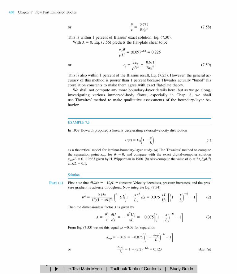
x (7.58)

This is within 1 percent of Blasius’ exact solution, Eq. (7.30).With 0, Eq. (7.56) predicts the flat-plate shear to be

w

U

(0.09)0.62 0.225

or cf

2Uw

2 (7.59)

This is also within 1 percent of the Blasius result, Eq. (7.25). However, the general ac-curacy of this method is poorer than 1 percent because Thwaites actually “tuned” hiscorrelation constants to make them agree with exact flat-plate theory.

We shall not compute any more boundary-layer details here, but as we go along,investigating various immersed-body flows, especially in Chap. 8, we shall use Thwaites’ method to make qualitative assessments of the boundary-layer be-havior.

EXAMPLE 7.5

In 1938 Howarth proposed a linearly decelerating external-velocity distribution

U(x) U01 Lx

(1)

as a theoretical model for laminar-boundary-layer study. (a) Use Thwaites’ method to computethe separation point xsep for 0 0, and compare with the exact digital-computer solutionxsep/L 0.119863 given by H. Wipperman in 1966. (b) Also compute the value of cf 2w/(U2)at x/L 0.1.

Solution

First note that dU/dx U0/L constant: Velocity decreases, pressure increases, and the pres-sure gradient is adverse throughout. Now integrate Eq. (7.54)

2 x

0U5

01 Lx

5

dx 0.075 UL

0 1

Lx

6

1 (2)

Then the dimensionless factor is given by

ddUx

2UL

0 0.0751 Lx

6

1 (3)

From Eq. (7.55) we set this equal to 0.09 for separation

sep 0.09 0.0751 6

1or 1 (2.2)1/6 0.123 Ans. (a)

xsep

L

xsep

L

2

v

0.45vU6

0(1 x/L)6

0.671Rex

1/2

0.671Rex

1/2


Part (b)

7.6 Experimental ExternalFlows

This is less than 3 percent higher than Wipperman’s exact solution, and the computational ef-fort is very modest.

To compute cf at x/L 0.1 (just before separation), we first compute at this point, using Eq. (3)

(x 0.1L) 0.075[(1 0.1)6 1] 0.0661

Then from Eq. (7.56) the shear parameter is

S(x 0.1L) (0.0661 0.09)0.62 0.099 12

cf Re (4)

We can compute Re in terms of ReL from Eq. (2) or (3)

L2

2 0U.0

L6/6

1

0.R06

eL

61

or Re 0.257 ReL1/2 at

Lx

0.1

Substitute into Eq. (4):

0.099 12

cf(0.257 ReL1/2)

or cf ReL U

L Ans. (b)

We cannot actually compute cf without the value of, say, U0L/.

Boundary-layer theory is very interesting and illuminating and gives us a great quali-tative grasp of viscous-flow behavior, but, because of flow separation, the theory doesnot generally allow a quantitative computation of the complete flow field. In particu-lar, there is at present no satisfactory theory for the forces on an arbitrary body im-mersed in a stream flowing at an arbitrary Reynolds number. Therefore experimenta-tion is the key to treating external flows.

Literally thousands of papers in the literature report experimental data on specificexternal viscous flows. This section gives a brief description of the following external-flow problems:

1. Drag of two-and three-dimensional bodies

a. Blunt bodies

b. Streamlined shapes

2. Performance of lifting bodies

a. Airfoils and aircraft

b. Projectiles and finned bodies

c. Birds and insects

For further reading see the goldmine of data compiled in Hoerner [12]. In later chap-ters we shall study data on supersonic airfoils (Chap. 9), open-channel friction (Chap.10), and turbomachinery performance (Chap. 11).

0.77ReL

1/2

7.6 Experimental External Flows 451

Fig. 7.10 Definition of forces andmoments on a body immersed in auniform flow.

Drag of Immersed Bodies Any body of any shape when immersed in a fluid stream will experience forces andmoments from the flow. If the body has arbitrary shape and orientation, the flow willexert forces and moments about all three coordinate axes, as shown in Fig. 7.10. It iscustomary to choose one axis parallel to the free stream and positive downstream. Theforce on the body along this axis is called drag, and the moment about that axis therolling moment. The drag is essentially a flow loss and must be overcome if the bodyis to move against the stream.

A second and very important force is perpendicular to the drag and usually performsa useful job, such as bearing the weight of the body. It is called the lift. The momentabout the lift axis is called yaw.

The third component, neither a loss nor a gain, is the side force, and about this axisis the pitching moment. To deal with this three-dimensional force-moment situation ismore properly the role of a textbook on aerodynamics [for example, 13]. We shall limitthe discussion here to lift and drag.

When the body has symmetry about the lift-drag axis, e.g., airplanes, ships, and carsmoving directly into a stream, the side force, yaw, and roll vanish, and the problem re-duces to a two-dimensional case: two forces, lift and drag, and one moment, pitch.

A final simplification often occurs when the body has two planes of symmetry, asin Fig. 7.11. A wide variety of shapes such as cylinders, wings, and all bodies of rev-olution satisfy this requirement. If the free stream is parallel to the intersection of thesetwo planes, called the principal chord line of the body, the body experiences drag only,with no lift, side force, or moments.4 This type of degenerate one-force drag data iswhat is most commonly reported in the literature, but if the free stream is not parallelto the chord line, the body will have an unsymmetric orientation and all three forcesand three moments can arise in principle.

In low-speed flow past geometrically similar bodies with identical orientation andrelative roughness, the drag coefficient should be a function of the body Reynolds num-ber

CD f(Re) (7.60)


Arbitrarybody

Lift force

Yawing moment Drag force

Rolling moment

Pitching moment

Side forceFreestream

velocity

V

4In bodies with shed vortices, such as the cylinder in Fig. 5.2, there may be oscillating lift, side force,and moments, but their mean value is zero.

Fig. 7.11 Only the drag force oc-curs if the flow is parallel to bothplanes of symmetry.

The Reynolds number is based upon the free-stream velocity V and a characteristiclength L of the body, usually the chord or body length parallel to the stream

Re V

L (7.61)

For cylinders, spheres, and disks, the characteristic length is the diameter D.

Drag coefficients are defined by using a characteristic area A which may differ de-pending upon the body shape:

CD (7.62)

The factor 12

is our traditional tribute to Euler and Bernoulli. The area A is usually oneof three types:

1. Frontal area, the body as seen from the stream; suitable for thick, stubby bodies,such as spheres, cylinders, cars, missiles, projectiles, and torpedoes.

2. Planform area, the body area as seen from above; suitable for wide, flat bodiessuch as wings and hydrofoils.

3. Wetted area, customary for surface ships and barges.

In using drag or other fluid-force data, it is important to note what length and area arebeing used to scale the measured coefficients.

As we have mentioned, the theory of drag is weak and inadequate, except for the flatplate. This is because of flow separation. Boundary-layer theory can predict the sepa-ration point but cannot accurately estimate the (usually low) pressure distribution inthe separated region. The difference between the high pressure in the front stagnationregion and the low pressure in the rear separated region causes a large drag contribu-tion called pressure drag. This is added to the integrated shear stress or friction dragof the body, which it often exceeds:

CD CD,press CD,fric (7.63)

drag

12

V2A


V

Vertical plane of symmetry Horizontal planeof symmetry

Principalchord line

Doublysymmetric

body

Drag only if Vis parallel tochord line

Characteristic Area

Friction Drag and Pressure Drag

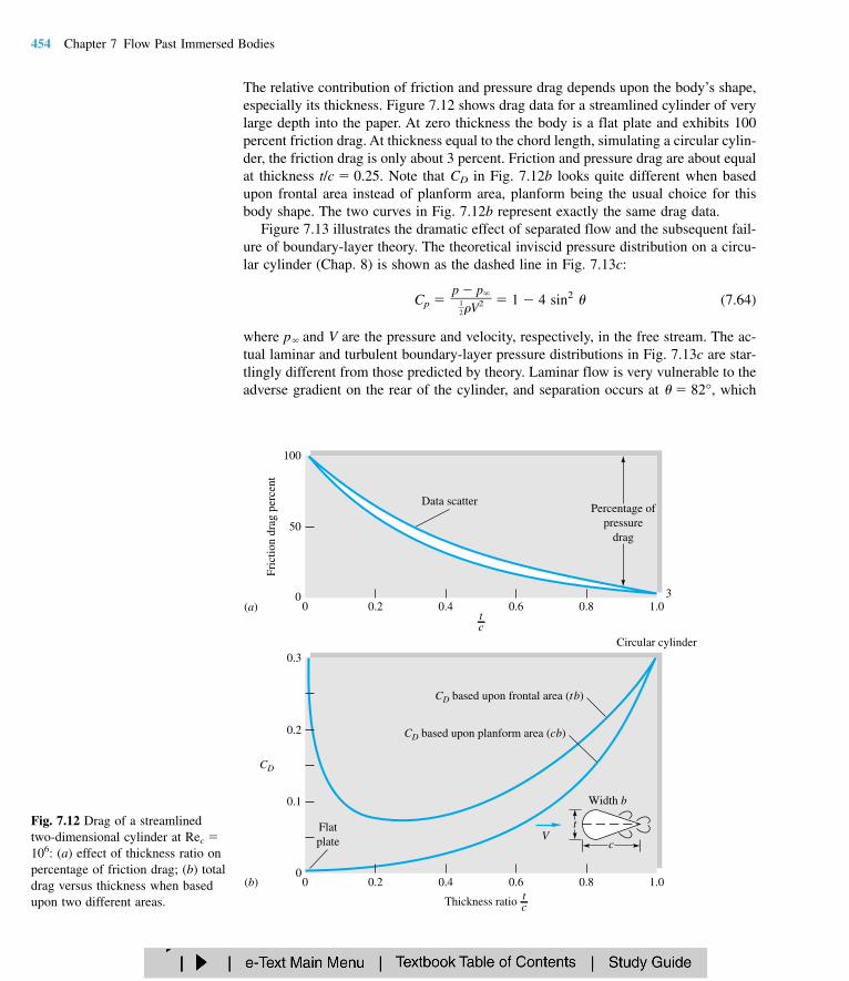
Fig. 7.12 Drag of a streamlinedtwo-dimensional cylinder at Rec 106: (a) effect of thickness ratio onpercentage of friction drag; (b) totaldrag versus thickness when basedupon two different areas.

The relative contribution of friction and pressure drag depends upon the body’s shape,especially its thickness. Figure 7.12 shows drag data for a streamlined cylinder of verylarge depth into the paper. At zero thickness the body is a flat plate and exhibits 100percent friction drag. At thickness equal to the chord length, simulating a circular cylin-der, the friction drag is only about 3 percent. Friction and pressure drag are about equalat thickness t/c 0.25. Note that CD in Fig. 7.12b looks quite different when basedupon frontal area instead of planform area, planform being the usual choice for thisbody shape. The two curves in Fig. 7.12b represent exactly the same drag data.

Figure 7.13 illustrates the dramatic effect of separated flow and the subsequent fail-ure of boundary-layer theory. The theoretical inviscid pressure distribution on a circu-lar cylinder (Chap. 8) is shown as the dashed line in Fig. 7.13c:

Cp 1 4 sin2 (7.64)

where p and V are the pressure and velocity, respectively, in the free stream. The ac-tual laminar and turbulent boundary-layer pressure distributions in Fig. 7.13c are star-tlingly different from those predicted by theory. Laminar flow is very vulnerable to theadverse gradient on the rear of the cylinder, and separation occurs at 82°, which

p p12

V2


0.3

0.2

0.1

00

CD

0.2 0.4 0.6 0.8 1.0

Circular cylinder

CD based upon frontal area (t b)

CD based upon planform area (c b)

Width b

tV

c

Thickness ratio tc

(b)

Flatplate

100

50

00 0.2 0.4 0.6 0.8 1.0(a)

3

Percentage ofpressure

drag

Data scatter

Fric

tion

drag

per

cent

tc

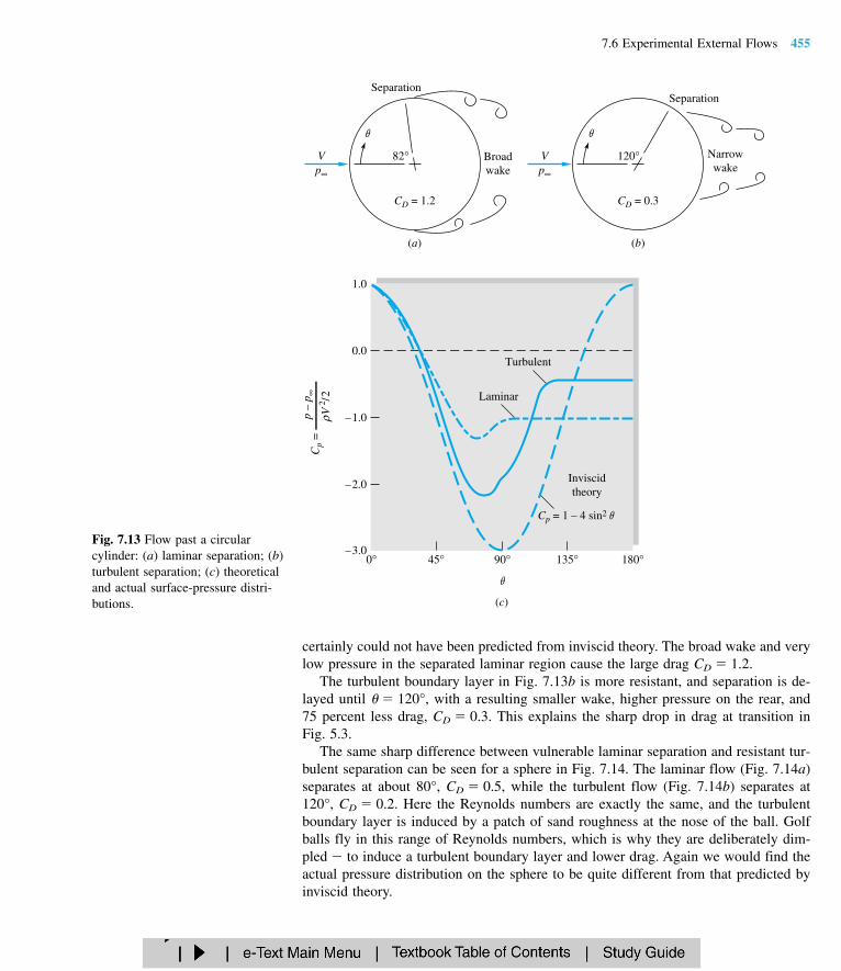
Fig. 7.13 Flow past a circularcylinder: (a) laminar separation; (b)turbulent separation; (c) theoreticaland actual surface-pressure distri-butions.

certainly could not have been predicted from inviscid theory. The broad wake and verylow pressure in the separated laminar region cause the large drag CD 1.2.

The turbulent boundary layer in Fig. 7.13b is more resistant, and separation is de-layed until 120°, with a resulting smaller wake, higher pressure on the rear, and75 percent less drag, CD 0.3. This explains the sharp drop in drag at transition inFig. 5.3.

The same sharp difference between vulnerable laminar separation and resistant tur-bulent separation can be seen for a sphere in Fig. 7.14. The laminar flow (Fig. 7.14a)separates at about 80°, CD 0.5, while the turbulent flow (Fig. 7.14b) separates at120°, CD 0.2. Here the Reynolds numbers are exactly the same, and the turbulentboundary layer is induced by a patch of sand roughness at the nose of the ball. Golfballs fly in this range of Reynolds numbers, which is why they are deliberately dim-pled to induce a turbulent boundary layer and lower drag. Again we would find theactual pressure distribution on the sphere to be quite different from that predicted byinviscid theory.


Separation

Vp∞

Broadwake

82°

CD = 1.2

(a)

θ

Separation

Vp∞

Narrowwake

120°

CD = 0.3

(b)

θ

1.0

0.0

– 1.0

– 2.0

– 3.00° 45° 90° 135° 180°

(c)

θ

Turbulent

Laminar

Inviscidtheory

θCp = 1 – 4 sin2

Cp

=p

– p ∞

ρ V

2 / 2

Fig. 7.14 Strong differences in lam-inar and turbulent separation on an8.5-in bowling ball entering waterat 25 ft/s: (a) smooth ball, laminarboundary layer; (b) same entry, tur-bulent flow induced by patch ofnose-sand roughness. (U.S. Navyphotograph, Ordnance Test Station,Pasadena Annex.)

In general, we cannot overstress the importance of body streamlining to reducedrag at Reynolds numbers above about 100. This is illustrated in Fig. 7.15. The rec-tangular cylinder (Fig. 7.15a) has rampant separation at all sharp corners and veryhigh drag. Rounding its nose (Fig. 7.15b) reduces drag by about 45 percent, but CD

is still high. Streamlining its rear to a sharp trailing edge (Fig. 7.15c) reduces its draganother 85 percent to a practical minimum for the given thickness. As a dramatic con-trast, the circular cylinder (Fig. 7.15d) has one-eighth the thickness and one-three-hundredth the cross section (c) (Fig. 7.15c), yet it has the same drag. For high-per-formance vehicles and other moving bodies, the name of the game is drag reduction,for which intense research continues for both aerodynamic and hydrodynamic appli-cations [20, 39].

The drag of some representative wide-span (nearly two-dimensional) bodies is shownversus the Reynolds number in Fig. 7.16a. All bodies have high CD at very low (creep-ing flow) Re 1.0, while they spread apart at high Reynolds numbers according to


(a ) (b )

V

(a)

CD = 1.1

V

(c)

CD = 2.0 V

(b)

CD = 0.15 V

(d )

Fig. 7.15 The importance ofstreamlining in reducing drag of abody (CD based on frontal area):(a) rectangular cylinder; (b)rounded nose; (c) rounded nose andstreamlined sharp trailing edge; (d)circular cylinder with the samedrag as case (c).

Fig. 7.16 Drag coefficients ofsmooth bodies at low Mach num-bers: (a) two-dimensional bodies;(b) three-dimensional bodies. Notethe Reynolds-number independenceof blunt bodies at high Re.

their degree of streamlining. All values of CD are based on the planform area exceptthe plate normal to the flow. The birds and the sailplane are, of course, not very two-dimensional, having only modest span length. Note that birds are not nearly as effi-cient as modern sailplanes or airfoils [14, 15].

Table 7.2 gives a few data on drag, based on frontal area, of two-dimensional bod-ies of various cross section, at Re 104. The sharp-edged bodies, which tend to causeflow separation regardless of the character of the boundary layer, are insensitive to theReynolds number. The elliptic cylinders, being smoothly rounded, have the laminar-to-turbulent transition effect of Figs. 7.13 and 7.14 and are therefore quite sensitive towhether the boundary layer is laminar or turbulent.


10

100

10

1

0.1

0.01

0.0010.1 1 10 100 10

3 10

4 10

5 10

6 10

7

Re

Airfoil

Seagull

Sailplane

CD

Stokes'law:

24/ReDisk

(a)

100

10

1

0.1

0.01

CD

0.1 1 100 10

3 10

4 10

5 10

6 10

7

Re

(b)

Smoothflat plateparallel

to stream

LD

= ∞= 5

Smoothcircularcylinder

Squarecylinder

Platenormal

to stream

Transition

Pigeon

Vulture

2:1ellipsoid

Airship hull

Sphere


Table 7.2 Drag of Two-Dimensional Bodies at Re 104

Square cylinder:

Half tube:

Half-cylinder:

Equilateral triangle:

2.1

1.6

1.2

2.3

1.2

1.7

1.6

2.0

2.0

1.4

1.0 0.7

Plate:

Thin plate normal to a wall:

Hexagon:

L

H

Rounded nose section:

0.51.16

1.00.90

2.00.70

4.00.68

6.00.64

H

L

Rounded nose section:

L/H:

0.11.9

0.42.3

0.72.7

1.22.1

2.01.8

2.51.4

3.01.3

6.00.9

Elliptical cylinder: Laminar

1.2

0.6

0.35

0.25

Turbulent

0.3

0.2

0.15

0.1

1:1

2:1

4:1

8:1

CD:

L/H: CD:

CD based CD based CD basedon frontal on frontal on frontal

Shape area Shape area Shape area

Shape CD based on frontal area

Flat nose section

L/H:

CD:

L/H:

CD:

Plate:

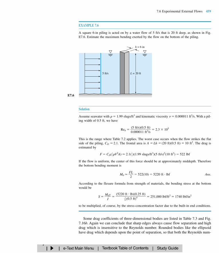
EXAMPLE 7.6

A square 6-in piling is acted on by a water flow of 5 ft/s that is 20 ft deep, as shown in Fig.E7.6. Estimate the maximum bending exerted by the flow on the bottom of the piling.


L = 20 ft5 ft/s

h = 6 in

E7.6

Solution

Assume seawater with 1.99 slugs/ft3 and kinematic viscosity 0.000011 ft2/s. With a pil-ing width of 0.5 ft, we have

Reh 0(5.0

f0t0/s0)1(01.5ft2

ft/)s

2.3 105

This is the range where Table 7.2 applies. The worst case occurs when the flow strikes the flatside of the piling, CD 2.1. The frontal area is A Lh (20 ft)(0.5 ft) 10 ft2. The drag isestimated by

F CD(12

V2A) 2.1(12

)(1.99 slugs/ft3)(5 ft/s)2(10 ft2) 522 lbf

If the flow is uniform, the center of this force should be at approximately middepth. Thereforethe bottom bending moment is

M0 F2L 522(10) 5220 ft lbf Ans.

According to the flexure formula from strength of materials, the bending stress at the bottomwould be

S M

I0y 251,000 lbf/ft2 1740 lbf/in2

to be multiplied, of course, by the stress-concentration factor due to the built-in end conditions.

Some drag coefficients of three-dimensional bodies are listed in Table 7.3 and Fig.7.16b. Again we can conclude that sharp edges always cause flow separation and highdrag which is insensitive to the Reynolds number. Rounded bodies like the ellipsoidhave drag which depends upon the point of separation, so that both the Reynolds num-

(5220 ft lb)(0.25 ft)

112(0.5 ft)4


Table 7.3 Drag of Three-Dimensional Bodies at Re 104

CD based onBody frontal area Body CD based on frontal area

Cube:

1.07

0.81

Cup:

1.4

0.4

1.17

Disk:

1.2

Parachute (Low porosity):

Rectangular plate:

h

b

h

b/h 15

1020∞

1.181.21.31.52.0

L/D:CD:

10.64

20.68

30.72

50.74

100.82

200.91

400.98

∞1.20

L

D

Short cylinder, laminar flow:

Porous parabolic dish [23]: Porosity: 0

1.420.95

0.11.330.92

0.21.200.90

0.31.050.86

0.40.950.83

0.50.820.80

Flat-faced cylinder:

Ellipsoid:

L /d 0.51248

1.150.900.850.870.99

L /d 0.75

Laminar

0.50.470.270.250.2

Turbulent

0.20.20.130.10.08

1248

d

L

CD

A ≈ 9 ft2 C D

A ≈ 1.2 ft2

Average person:

U, m/s:CD:

101.2 ± 0.2

201.0 ± 0.2

300.7 ± 0.2

400.5 ± 0.2

Pine and spruce trees [24]:

L

d

Cone:10˚0.30

20˚0.40

30˚0.55

40˚0.65

60˚0.80

75˚1.05

90˚1.15

θθ :CD:

CD:

CD:

CD based on CD based onBody Ratio frontal area Body Ratio frontal area

Aerodynamic Forces on RoadVehicles

Fig. 7.17 Aerodynamics of automo-biles: (a) the historical trend fordrag coefficients [From Ref. 21];(b) effect of bottom rear upsweepangle on drag and downward liftforce [From Ref. 25].

ber and the character of the boundary layer are important. Body length will generally de-crease pressure drag by making the body relatively more slender, but sooner or later thefriction drag will catch up. For the flat-faced cylinder in Table 7.3, pressure drag decreaseswith L/d but friction increases, so that minimum drag occurs at about L/d 2.

Automobiles and trucks are now the subject of much research on aerodynamic forces,both lift and drag [21]. At least one textbook is devoted to the subject [22]. Consumer,manufacturer, and government interest has cycled between high speed/high horsepowerand lower speed/lower drag. Better streamlining of car shapes has resulted over theyears in a large decrease in the automobile drag coefficient, as shown in Fig. 7.17a.Modern cars have an average drag coefficient of about 0.35, based upon the frontal


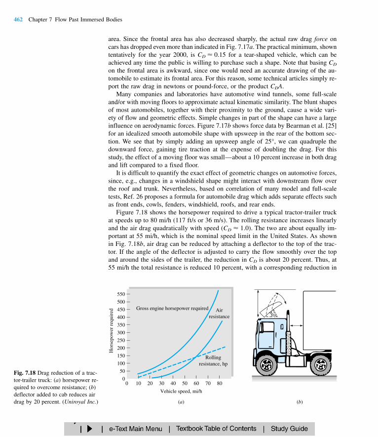
Fig. 7.18 Drag reduction of a trac-tor-trailer truck: (a) horsepower re-quired to overcome resistance; (b)deflector added to cab reduces airdrag by 20 percent. (Uniroyal Inc.)

area. Since the frontal area has also decreased sharply, the actual raw drag force oncars has dropped even more than indicated in Fig. 7.17a. The practical minimum, showntentatively for the year 2000, is CD 0.15 for a tear-shaped vehicle, which can beachieved any time the public is willing to purchase such a shape. Note that basing CD

on the frontal area is awkward, since one would need an accurate drawing of the au-tomobile to estimate its frontal area. For this reason, some technical articles simply re-port the raw drag in newtons or pound-force, or the product CDA.

Many companies and laboratories have automotive wind tunnels, some full-scaleand/or with moving floors to approximate actual kinematic similarity. The blunt shapesof most automobiles, together with their proximity to the ground, cause a wide vari-ety of flow and geometric effects. Simple changes in part of the shape can have a largeinfluence on aerodynamic forces. Figure 7.17b shows force data by Bearman et al. [25]for an idealized smooth automobile shape with upsweep in the rear of the bottom sec-tion. We see that by simply adding an upsweep angle of 25°, we can quadruple thedownward force, gaining tire traction at the expense of doubling the drag. For thisstudy, the effect of a moving floor was small—about a 10 percent increase in both dragand lift compared to a fixed floor.

It is difficult to quantify the exact effect of geometric changes on automotive forces,since, e.g., changes in a windshield shape might interact with downstream flow overthe roof and trunk. Nevertheless, based on correlation of many model and full-scaletests, Ref. 26 proposes a formula for automobile drag which adds separate effects suchas front ends, cowls, fenders, windshield, roofs, and rear ends.

Figure 7.18 shows the horsepower required to drive a typical tractor-trailer truckat speeds up to 80 mi/h (117 ft/s or 36 m/s). The rolling resistance increases linearlyand the air drag quadratically with speed (CD 1.0). The two are about equally im-portant at 55 mi/h, which is the nominal speed limit in the United States. As shownin Fig. 7.18b, air drag can be reduced by attaching a deflector to the top of the trac-tor. If the angle of the deflector is adjusted to carry the flow smoothly over the topand around the sides of the trailer, the reduction in CD is about 20 percent. Thus, at55 mi/h the total resistance is reduced 10 percent, with a corresponding reduction in


Hor

sepo

wer

req

uire

d

0 20 30 40 50 60 70 8010

Vehicle speed, mi/h

(a) (b)

Gross engine horsepower required Airresistance

Rollingresistance, hp

550

500

450

400

350

300

250

200

150

100

50

0

E7.7

fuel costs and/or trip time for the trucker. This type of applied fluids engineering canbe a large factor in many of the conservation-oriented transportation problems of thefuture.

EXAMPLE 7.7

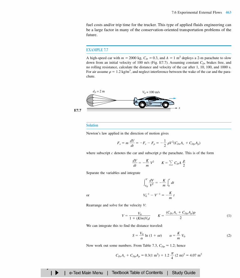
A high-speed car with m 2000 kg, CD 0.3, and A 1 m2 deploys a 2-m parachute to slowdown from an initial velocity of 100 m/s (Fig. E7.7). Assuming constant CD, brakes free, andno rolling resistance, calculate the distance and velocity of the car after 1, 10, 100, and 1000 s.For air assume 1.2 kg/m3, and neglect interference between the wake of the car and the para-chute.


d p = 2 m V0 = 100 m/s

x

Solution

Newton’s law applied in the direction of motion gives

Fx m ddVt Fc Fp

12

V 2(CDcAc CDpAp)

where subscript c denotes the car and subscript p the parachute. This is of the form

ddVt

mK

V2 K CDA

2

Separate the variables and integrate

V

V0

dVV2

mK

t

0dt

or V01 V1

mK

t

Rearrange and solve for the velocity V:

V 1 (K

V0

/m)V0t K (1)

We can integrate this to find the distance traveled:

S V

0 ln (1 t) mK

V0 (2)

Now work out some numbers. From Table 7.3, CDp 1.2; hence

CDcAc CDpAp 0.3(1 m2) 1.2

4 (2 m)2 4.07 m2

(CDc Ac CDpAp)

2

Other Methods of Drag Reduction

Drag of Surface Ships

Then mK

V0 0.122 s1

Now make a table of the results for V and S from Eqs. (1) and (2):

t, s 1 10 100 1000

V, m/s 89 45 7.6 0.8

S, m 94 654 2110 3940

Air resistance alone will not stop a body completely. If you don’t apply the brakes, you’ll behalfway to the Yukon Territory and still going.

Sometimes drag is good, for example, when using a parachute. Do not jump out of anairplane holding a flat plate parallel to your motion (see Prob. 7.81). Mostly, though,drag is bad and should be reduced. The classical method of drag reduction is stream-lining (Figs. 7.15 and 7.18). For example, nose fairings and body panels have producedmotorcycles which can travel over 200 mi/h. More recent research has uncovered othermethods which hold great promise, especially for turbulent flows.

1. Oil pipelines introduce an annular core of water to reduce the pumping power[36]. The low-viscosity water rides the wall and reduces friction up to 60 per-cent.

2. Turbulent friction in liquid flows is reduced up to 60 percent by dissolving smallamounts of a high-molecular-weight polymer additive [37]. Without changingpumps, the Trans-Alaska Pipeline System (TAPS) increased oil flow 50 percentby injecting small amounts of polymer dissolved in kerosene.

3. Stream-oriented surface vee-groove microriblets reduce turbulent friction up to 8percent [38]. Riblet heights are of order 1 mm and were used on the Stars andStripes yacht hull in the Americas Cup races. Riblets are also effective on air-craft skins.

4. Small, near-wall large-eddy breakup devices (LEBUs) reduce local turbulentfriction up to 10 percent [39]. However, one must add these small structures tothe surface.

5. Air microbubbles injected at the wall of a water flow create a low-shear bubbleblanket [40]. At high void fractions, drag reduction can be 80 percent.

6. Spanwise (transverse) wall oscillation may reduce turbulent friction up to 30percent [41].

Drag reduction is presently an area of intense and fruitful research and applies to manytypes of airflows and water flows for both vehicles and conduits.

The drag data above, such as Tables 7.2 and 7.3, are for bodies “fully immersed” in afree stream, i.e., with no free surface. If, however, the body moves at or near a free liq-uid surface, wave-making drag becomes important and is dependent upon both theReynolds number and the Froude number. To move through a water surface, a ship

12

(4.07 m2)(1.2 kg/m3)(100 m/s)

2000 kg


Body Drag at High MachNumbers

must create waves on both sides. This implies putting energy into the water surfaceand requires a finite drag force to keep the ship moving, even in a frictionless fluid.The total drag of a ship can then be approximated as the sum of friction drag and wave-making drag:

F Ffric Fwave or CD CD,fric CD,wave

The friction drag can be estimated by the (turbulent) flat-plate formula, Eq. (7.45),based on the below-water or wetted area of the ship.

Reference 27 is an interesting review of both theory and experiment for wake-making surface ship drag. Generally speaking, the bow of the ship creates a wave sys-tem whose wavelength is related to the ship speed but not necessarily to the ship length.If the stern of the ship is a wave trough, the ship is essentially climbing uphill and hashigh wave drag. If the stern is a wave crest, the ship is nearly level and has lower drag.The criterion for these two conditions results in certain approximate Froude numbers[27]:

high drag if N 1, 3, 5, 7, . . . ;Fr (7.65)

low drag if N 2, 4, 6, 8, . . .

where V is the ship’s speed, L is the ship’s length along the centerline, and N is thenumber of half-lengths, from bow to stern, of the drag-making wave system. The wavedrag will increase with the Froude number and oscillate between lower drag (Fr 0.38, 0.27, 0.22, . . .) and higher drag (Fr 0.53, 0.31, 0.24, . . .) with negligible vari-ation for Fr 0.2. Thus it is best to design a ship to cruise at N 2, 4, 6, 8. Shapingthe bow and stern can further reduce wave-making drag.

Figure 7.19 shows the data of Inui [27] for a model ship. The main hull, curve A,shows peaks and valleys in wave drag at the appropriate Froude numbers 0.2. In-troduction of a bulb protrusion on the bow, curve B, greatly reduces the drag. Addinga second bulb to the stern, curve C, is still better, and Inui recommends that the designspeed of this two-bulb ship be at N 4, Fr 0.27, which is a nearly “waveless” con-dition. In this figure CD,wave is defined as 2Fwave/(V2L2) instead of using the wettedarea.

The solid curves in Fig. 7.19 are based on potential-flow theory for the below-water hull shape. Chapter 8 is an introduction to potential-flow theory. Modern digitalcomputers can be programmed for numerical CFD solutions of potential flow over thehulls of ships, submarines, yachts, and sailboats, including boundary-layer effects driven by the potential flow [28]. Thus theoretical prediction of flow past surface shipsis now at a fairly high level. See also Ref. 15.

All the data presented above are for nearly incompressible flows, with Mach numbersassumed less than about 0.5. Beyond this value compressibility can be very important,with CD fcn(Re, Ma). As the stream Mach number increases, at some subsonic valueMcrit 1 which depends upon the body’s bluntness and thickness, the local velocity atsome point near the body surface will become sonic. If Ma increases beyond Macrit,shock waves form, intensify, and spread, raising surface pressures near the front of thebody and therefore increasing the pressure drag. The effect can be dramatic with CD

0.53N

VgL


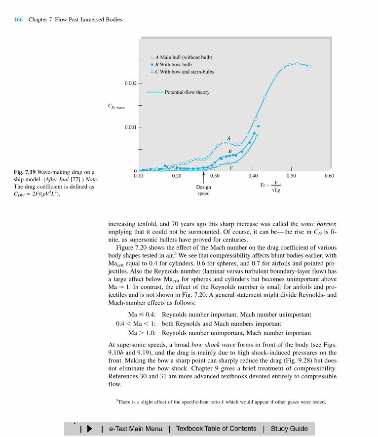
Fig. 7.19 Wave-making drag on aship model. (After Inui [27].) Note:The drag coefficient is defined asCDW 2F/(V2L2).

increasing tenfold, and 70 years ago this sharp increase was called the sonic barrier,implying that it could not be surmounted. Of course, it can be—the rise in CD is fi-nite, as supersonic bullets have proved for centuries.

Figure 7.20 shows the effect of the Mach number on the drag coefficient of variousbody shapes tested in air.5 We see that compressibility affects blunt bodies earlier, withMacrit equal to 0.4 for cylinders, 0.6 for spheres, and 0.7 for airfoils and pointed pro-jectiles. Also the Reynolds number (laminar versus turbulent boundary-layer flow) hasa large effect below Macrit for spheres and cylinders but becomes unimportant aboveMa 1. In contrast, the effect of the Reynolds number is small for airfoils and pro-jectiles and is not shown in Fig. 7.20. A general statement might divide Reynolds- andMach-number effects as follows:

Ma 0.4: Reynolds number important, Mach number unimportant

0.4 Ma 1: both Reynolds and Mach numbers important

Ma 1.0: Reynolds number unimportant, Mach number important

At supersonic speeds, a broad bow shock wave forms in front of the body (see Figs.9.10b and 9.19), and the drag is mainly due to high shock-induced pressures on thefront. Making the bow a sharp point can sharply reduce the drag (Fig. 9.28) but doesnot eliminate the bow shock. Chapter 9 gives a brief treatment of compressibility.References 30 and 31 are more advanced textbooks devoted entirely to compressibleflow.


0.10 0.20 0.30 0.40 0.50

Designspeed

Potential-flow theory

A Main hull (without bulb)B With bow-bulb

C With bow and stern-bulbs

A

B

C

Fr = V

√Lg

0.002

0.001

0

CD, wave

0.60

5There is a slight effect of the specific-heat ratio k which would appear if other gases were tested.

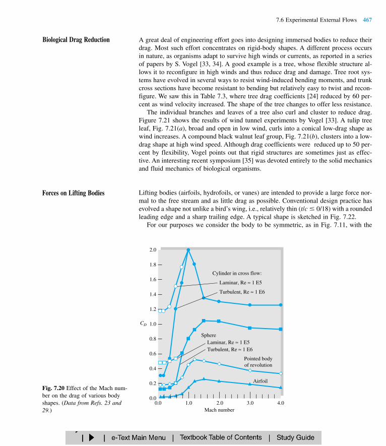
Fig. 7.20 Effect of the Mach num-ber on the drag of various bodyshapes. (Data from Refs. 23 and29.)

Biological Drag Reduction A great deal of engineering effort goes into designing immersed bodies to reduce theirdrag. Most such effort concentrates on rigid-body shapes. A different process occursin nature, as organisms adapt to survive high winds or currents, as reported in a seriesof papers by S. Vogel [33, 34]. A good example is a tree, whose flexible structure al-lows it to reconfigure in high winds and thus reduce drag and damage. Tree root sys-tems have evolved in several ways to resist wind-induced bending moments, and trunkcross sections have become resistant to bending but relatively easy to twist and recon-figure. We saw this in Table 7.3, where tree drag coefficients [24] reduced by 60 per-cent as wind velocity increased. The shape of the tree changes to offer less resistance.

The individual branches and leaves of a tree also curl and cluster to reduce drag.Figure 7.21 shows the results of wind tunnel experiments by Vogel [33]. A tulip treeleaf, Fig. 7.21(a), broad and open in low wind, curls into a conical low-drag shape aswind increases. A compound black walnut leaf group, Fig. 7.21(b), clusters into a low-drag shape at high wind speed. Although drag coefficients were reduced up to 50 per-cent by flexibility, Vogel points out that rigid structures are sometimes just as effec-tive. An interesting recent symposium [35] was devoted entirely to the solid mechanicsand fluid mechanics of biological organisms.

Lifting bodies (airfoils, hydrofoils, or vanes) are intended to provide a large force nor-mal to the free stream and as little drag as possible. Conventional design practice hasevolved a shape not unlike a bird’s wing, i.e., relatively thin (t/c 0/18) with a roundedleading edge and a sharp trailing edge. A typical shape is sketched in Fig. 7.22.

For our purposes we consider the body to be symmetric, as in Fig. 7.11, with the


0.0 1.0 2.0 3.0 4.0Mach number

Airfoil

Pointed bodyof revolution

SphereLaminar, Re ≈ 1 E5Turbulent, Re ≈ 1 E6

CD

Laminar, Re ≈ 1 E5

Turbulent, Re ≈ 1 E6

Cylinder in cross flow:

2.0

1.8

1.6

1.4

1.2

1.0

0.8

0.6

0.4

0.2

0.0

Forces on Lifting Bodies

Fig. 7.22 Definition sketch for alifting vane.

Fig. 7.21 Biological adaptation towind forces: (a) a tulip tree leafcurls into a conical shape at highvelocity; (b) black walnut leavescluster into a low-drag shape aswind increases. (From Vogel, Ref.33.)

free-stream velocity in the vertical plane. If the chord line between the leading andtrailing edge is not a line of symmetry, the airfoil is said to be cambered. The camberline is the line midway between the upper and lower surfaces of the vane.

The angle between the free stream and the chord line is called the angle of attack. The lift L and the drag D vary with this angle. The dimensionless forces are definedwith respect to the planform area Ap bc:

Lift coefficient: CL (7.66a)

Drag coefficient: CD (7.66b)D

12

V2Ap

L

12

V2Ap


5 m/s

10 m/s

20 m/s

(a)

5 m/s

10 m/s

20 m/s

(b)

α

Planformarea = bc

Angle ofattack

V

c = chord

b = spant = thickness

Lift

Drag

Fig. 7.23 Transient stages in thedevelopment of lift: (a) start-up:rear stagnation point on the uppersurface: no lift; (b) sharp trailingedge induces separation, and astarting vortex forms: slight lift; (c)starting vortex is shed, and stream-lines flow smoothly from trailingedge: lift is now 80 percent devel-oped; (d) starting vortex now shedfar behind, trailing edge now verysmooth: lift fully developed.

If the chord length is not constant, as in the tapered wings of modern aircraft,Ap c db.

For low-speed flow with a given roughness ratio, CL and CD should vary with andthe chord Reynolds number

CL f(, Rec) or CD f(, Rec)

where Rec Vc/. The Reynolds numbers are commonly in the turbulent-boundary-layer range and have a modest effect.

The rounded leading edge prevents flow separation there, but the sharp trailing edgecauses a separation which generates the lift. Figure 7.23 shows what happens when aflow starts up past a lifting vane or an airfoil.

Just after start-up in Fig. 7.23a the streamline motion is irrotational and inviscid.The rear stagnation point, assuming a positive angle of attack, is on the upper surface,and there is no lift; but the flow cannot long negotiate the sharp turn at the trailingedge: it separates, and a starting vortex forms in Fig. 7.23b. This starting vortex is sheddownstream in Fig. 7.23c and d, and a smooth streamline flow develops over the wing,leaving the foil in a direction approximately parallel to the chord line. Lift at this timeis fully developed, and the starting vortex is gone. Should the flow now cease, a stop-ping vortex of opposite (clockwise) sense will form and be shed. During flight, in-creases or decreases in lift will cause incremental starting or stopping vortices, alwayswith the effect of maintaining a smooth parallel flow at the trailing edge. We pursuethis idea mathematically in Chap. 8.

At a low angle of attack, the rear surfaces have an adverse pressure gradient but notenough to cause significant boundary-layer separation. The flow pattern is smooth, asin Fig. 7.23d, and drag is small and lift excellent. As the angle of attack is increased,the upper-surface adverse gradient becomes stronger, and generally a separation bub-


(a)

(b)

(c)

(d )

Fig. 7.24 At high angle of attack,smoke-flow visualization showsstalled flow on the upper surface ofa lifting vane. [From Ref. 19, Illus-trated Experiments in Fluid Me-chanics (The NCFMF Book of FilmNotes), National Committee forFluid Mechanics Films, EducationDevelopment Center, Inc., copy-right 1972.]

ble begins to creep forward on the upper surface.6 At a certain angle 15 to 20°,the flow is separated completely from the upper surface, as in Fig. 7.24. The airfoil issaid to be stalled: Lift drops off markedly, drag increases markedly, and the foil is nolonger flyable.

Early airfoils were thin, modeled after birds’ wings. The German engineer OttoLilienthal (1848–1896) experimented with flat and cambered plates on a rotating arm.He and his brother Gustav flew the world’s first glider in 1891. Horatio FrederickPhillips (1845–1912) built the first wind tunnel in 1884 and measured the lift and dragof cambered vanes. The first theory of lift was proposed by Frederick W. Lanchestershortly afterward. Modern airfoil theory dates from 1905, when the Russian hydrody-namicist N. E. Joukowsky (1847–1921) developed a circulation theorem (Chap. 8) forcomputing airfoil lift for arbitrary camber and thickness. With this basic theory, as ex-tended and developed by Prandtl and Kármán and their students, it is now possible todesign a low-speed airfoil to satisfy particular surface-pressure distributions and bound-ary-layer characteristics. There are whole families of airfoil designs, notably those de-veloped in the United States under the sponsorship of the NACA (now NASA). Ex-tensive theory and data on these airfoils are contained in Ref. 16. We shall discuss thisfurther in Chap. 8.

Figure 7.25 shows the lift and drag on a symmetric airfoil denoted as the NACA0009 foil, the last digit indicating the thickness of 9 percent. With no flap extended,


6For some airfoils the bubble leaps, not creeps, forward, and stall occurs rapidly and dangerously.

Fig. 7.25 Lift and drag of a sym-metric NACA 0009 airfoil of infi-nite span, including effect of asplit-flap deflection. Note thatroughness can increase CD from100 to 300 percent.

this airfoil, as expected, has zero lift at zero angle of attack. Up to about 12° the liftcoefficient increases linearly with a slope of 0.1 per degree, or 6.0 per radian. This isin agreement with the theory outlined in Chap. 8:

CL,theory 2 sin 2ch (7.67)

where h/c is the maximum camber expressed as a fraction of the chord. The NACA0009 has zero camber; hence CL 2 sin 0.11, where is in degrees. This isexcellent agreement.

The drag coefficient of the smooth-model airfoils in Fig. 7.25 is as low as 0.005,which is actually lower than both sides of a flat plate in turbulent flow. This is mis-leading inasmuch as a commercial foil will have roughness effects; e.g., a paint jobwill double the drag coefficient.

The effect of increasing Reynolds number in Fig. 7.25 is to increase the maximumlift and stall angle (without changing the slope appreciably) and to reduce the drag co-efficient. This is a salutary effect, since the prototype will probably be at a higherReynolds number than the model (107 or more).

For takeoff and landing, the lift is greatly increased by deflecting a split flap, asshown in Fig. 7.25. This makes the airfoil unsymmetric (or effectively cambered) andchanges the zero-lift point to 12°. The drag is also greatly increased by the flap,but the reduction in takeoff and landing distance is worth the extra power needed.

A lifting craft cruises at low angle of attack, where the lift is much larger than thedrag. Maximum lift-to-drag ratios for the common airfoils lie between 20 and 50.

Some airfoils, such as the NACA 6 series, are shaped to provide favorable gradi-ents over much of the upper surface at low angles. Thus separation is small, and tran-sition to turbulence is delayed; the airfoil retains a good length of laminar flow even


CL

α

6 × 10

6

3 × 10 6

–12 – 8 – 4

CD

– 8 – 4 0 4 8 12 160 4 8 12 16

, degα , degα

1.6

1.2

0.8

0.4

With flapat 60°

Rec = 6 × 10

6

No flap

No flap

0.01

0.02

0.03

0.04

Splitflap

Rec = 9 × 10

6

With flapat 60°

Rec = 3 × 10

6

6 × 10

6

9 × 10

6

Fig. 7.26 Lift-drag polar plot forstandard (0009) and a laminar-flow(63-009) NACA airfoil.

at high Reynolds numbers. The lift-drag polar plot in Fig. 7.26 shows the NACA 0009data from Fig. 7.25 and a laminar-flow airfoil, NACA 63–009, of the same thickness.The laminar-flow airfoil has a low-drag bucket at small angles but also suffers lowerstall angle and lower maximum lift coefficient. The drag is 30 percent less in the bucket,but the bucket disappears if there is significant surface roughness.

All the data in Figs. 7.25 and 7.26 are for infinite span, i.e., a two-dimensional flowpattern about wings without tips. The effect of finite span can be correlated with thedimensionless slenderness, or aspect ratio, denoted (AR),

AR Ab2

p

bc

(7.68)

where c is the average chord length. Finite-span effects are shown in Fig. 7.27. Thelift slope decreases, but the zero-lift angle is the same; and the drag increases, but thezero-lift drag is the same. The theory of finite-span airfoils [16] predicts that the ef-fective angle of attack increases, as in Fig. 7.27, by the amount

!

CA

L

R (7.69)

When applied to Eq. (7.67), the finite-span lift becomes

CL 2 s1in

(2/

AR2h/c)

(7.70)

The associated drag increase is !CD CL sin ! CL !, or

CD CD (7.71)CL

2

AR


1.2

0.8

0.4

00

0.008 0.016 0.024

CL

Stall

CD

Low-drag“bucket”

NACA0009

NACA63 – 009

0009 withsplit flap

Stall

Fig. 7.27 Effect of finite aspect ra-tio on lift and drag of an airfoil: (a)effective angle increase; (b) in-duced drag increase.

where CD is the drag of the infinite-span airfoil, as sketched in Fig. 7.25. These cor-relations are in good agreement with experiments on finite-span wings [16].

The existence of a maximum lift coefficient implies the existence of a minimumspeed, or stall speed, for a craft whose lift supports its weight

L W CL,max(12

Vs2Ap)

or Vs 1/2

(7.72)

The stall speed of typical aircraft varies between 60 and 200 ft/s, depending upon theweight and value of CL,max. The pilot must hold the speed greater than about 1.2Vs toavoid the instability associated with complete stall.

The split flap in Fig. 7.25 is only one of many devices used to secure high lift atlow speeds. Figure 7.28a shows six such devices whose lift performance is given in7.28b along with a standard (A) and laminar-flow (B) airfoil. The double-slotted flapachieves CL,max 3.4, and a combination of this plus a leading-edge slat can achieveCL,max 4.0. These are not scientific curiosities; e.g., the Boeing 727 commercial jetaircraft uses a triple-slotted flap plus a leading-edge slat during landing.

Also shown as C in Fig. 7.28b is the Kline-Fogleman airfoil [17], not yet a reality.The designers are amateur model-plane enthusiasts who did not know that conventionalaerodynamic wisdom forbids a sharp leading edge and a step cutout from the trailingedge. The Kline-Fogleman airfoil has relatively high drag but shows an amazing con-tinual increase in lift out to 45°. In fact, we may fairly say that this airfoil doesnot stall and provides smooth performance over a tremendous range of flight condi-tions. No explanation for this behavior has yet been published by any aerodynamicist.This airfoil is under study and may or may not have any commercial value.

Another violation of conventional aerodynamic wisdom is that military aircraft arebeginning to fly, briefly, above the stall point. Fighter pilots are learning to make quickmaneuvers in the stalled region as detailed in Ref. 32. Some planes can even fly con-tinuously while stalled—the Grumman X-29 experimental aircraft recently set a recordby flying at 67°.

2WCL,maxAp


CLAR = ∞

AR =A p

b

2

(a)

CD

AR =A p

b

2

AR = ∞

α

∆ CD ≈CL

π AR

2

(b)

CD ∞

β–

CL

π AR∆ ≈α

α

Fig. 7.29 New aircraft designs donot necessarily look like your typi-cal jetliner. (From Ref. 42.)

Fig. 7.28 Performance of airfoilswith and without high-lift devices:A NACA 0009; B NACA 63-009; C Kline-Fogleman airfoil(from Ref. 17); D to I shown in (a):(a) types of high-lift devices; (b)lift coefficients for various devices.

The Kline-Fogleman airfoil in Fig. 7.28 is a departure from conventional aerodynamics,but there have been other striking departures, as detailed in a recent article [42]. Thesenew aircraft, conceived presently as small models, have a variety of configurations, asshown in Fig. 7.29: ring-wing, cruciform, flying saucer, and flap-wing. A saucer config-uration (Fig. 7.29c), with a diameter of 40 in, has been successfully flown by radio con-trol, and its inventor, Jack M. Jones, plans for a 20-ft two-passenger version. Another 18-in-span microplane called the Bat (not shown), made by MLB Co., flies for 20 min at40 mi/h and contains a video camera for surveillance. New engines have been reducedto a 10- by 3-mm size, producing 20 W of power. At the other end of the size spectrum,Boeing and NASA engineers have proposed a jumbo flying-wing jetliner, similar in shapeto the stealth bomber, which would carry 800 passengers for a range of 7000 mi.

Further information on the performance of lifting craft can be found in Refs. 12,13, and 16. We discuss this matter again briefly in Chap. 8.


Plain flap or aileron

Split flap

External airfoil flap

Slotted flap

Double-slotted flap

Leading edge slat

(a)

D

E

F

G

H

I

Optimum butcumbersomecombination

Kline-Fogleman

airfoil

α, deg

(b)

CL

4

3

2

1

0– 10 10 20 30 40 50°

H

G

F

E, D

I

A

B

C

New Aircraft Designs

(a) Ring-wing (b) Cruciform delta

(c) Flying saucer (d) Flap-wing dragonfly

EXAMPLE 7.8

An aircraft weighs 75,000 lb, has a planform area of 2500 ft2, and can deliver a constantthrust of 12,000 lb. It has an aspect ratio of 7, and CD 0.02. Neglecting rolling resistance,estimate the takeoff distance at sea level if takeoff speed equals 1.2 times stall speed. TakeCL,max 2.0.

Solution

The stall speed from Eq. (7.72), with sea-level density 0.00237 slug/ft3, is

Vs 1/2

1/2

112.5 ft/s

Hence takeoff speed V0 1.2Vs 135 ft/s. The drag is estimated from Eq. (7.71) for AR 7 as

CD 0.02 0.02 0.0455CL2

A force balance in the direction of takeoff gives

Fs m ddVt thrust drag T kV2 k

12

CDAp (1)

Since we are looking for distance, not time, we introduce dV/dt V dV/ds into Eq. (1), sepa-rate variables, and integrate

S0

0dS

m2

V0

0k const

or S0 2mk ln

2mk ln (2)

where D0 kV02 is the takeoff drag. Equation (2) is the desired theoretical relation for takeoff

distance. For the particular numerical values, take

m 753,20.020

2329 slugs

CL0 1.39

CD0 0.02 0.0455(CL0

)2 0.108

k 12

CD0Ap (

12

)(0.108)(0.00237)(2500) 0.319 slug/ft

D0 kV02 5820 lb

Then Eq. (2) predicts that

S0 2(0

2.332199

sslluuggs/ft)

ln 12,0

1020,0

005820

3650 ln 1.94 2420 ft Ans.

A more exact analysis accounting for variable k [13] gives the same result to within 1 percent.

75,000

12

(0.00237)(135)2(2500)W

12

V02 Ap

TT D0

TT kV0

2

d(V2)T kV2

CL2

7

2(75,000)2.0(0.00237)(2500)

2WCL,maxAp


Summary This chapter has dealt with viscous effects in external flow past bodies immersed in astream. When the Reynolds number is large, viscous forces are confined to a thin bound-ary layer and wake in the vicinity of the body. Flow outside these “shear layers” is es-sentially inviscid and can be predicted by potential theory and Bernoulli’s equation.

The chapter begins with a discussion of the flat-plate boundary layer and the use ofmomentum-integral estimates to predict the wall shear, friction drag, and thickness ofsuch layers. These approximations suggest how to eliminate certain small terms in theNavier-Stokes equations, resulting in Prandtl’s boundary-layer equations for laminarand turbulent flow. Section 7.4 then solves the boundary-layer equations to give veryaccurate formulas for flat-plate flow at high Reynolds numbers. Rough-wall effects areincluded, and Sec. 7.5 gives a brief introduction to pressure-gradient effects. An ad-verse (decelerating) gradient is seen to cause flow separation, where the boundary layerbreaks away from the surface and forms a broad, low-pressure wake.

Boundary-layer theory fails in separated flows, which are commonly studied by experiment. Section 7.6 gives data on drag coefficients of various two- and three-dimensional body shapes. The chapter ends with a brief discussion of lift forces gen-erated by lifting bodies such as airfoils and hydrofoils. Airfoils also suffer flow sepa-ration or stall at high angles of incidence.


Problems

Most of the problems herein are fairly straightforward. More dif-ficult or open-ended assignments are labeled with an asterisk. Prob-lems labeled with an EES icon will benefit from the use of the En-gineering Equation Solver (EES), while problems labeled with acomputer disk may require the use of a computer. The standardend-of-chapter problems 7.1 to 7.124 (categorized in the problemlist below) are followed by word problems W7.1 to W7.12, fun-damentals of engineering exam problems FE7.1 to FE7.10, com-prehensive problems C7.1 to C7.4, and design project D7.1.

Problem Distribution

Section Topic Problems

7.1 Reynolds-number and geometry 7.1–7.57.2 Momentum-integral estimates 7.6–7.127.3 The boundary-layer equations 7.13–7.157.4 Laminar flat-plate flow 7.16–7.297.4 Turbulent flat-plate flow 7.30–7.467.5 Boundary layers with pressure gradient 7.47–7.527.6 Drag of two-dimensional bodies 7.53–7.637.6 Drag of three-dimensional bodies 7.64–7.1147.6 Lifting bodies—airfoils 7.115–7.124

P7.1 For flow at 20 m/s past a thin flat plate, estimate the dis-tances x from the leading edge at which the boundary-layerthickness will be either 1 mm or 10 cm for (a) air and (b)water at 20°C and 1 atm.

P7.2 Air, equivalent to that at a standard altitude of 4000 m,flows at 450 mi/h past a wing which has a thickness of 18

cm, a chord length of 1.5 m, and a wingspan of 12 m. Whatis the appropriate value of the Reynolds number for cor-relating the lift and drag of this wing? Explain your se-lection.

P7.3 Equation (7.1b) assumes that the boundary layer on theplate is turbulent from the leading edge onward. Devisea scheme for determining the boundary-layer thicknessmore accurately when the flow is laminar up to a pointRex,crit and turbulent thereafter. Apply this scheme to com-putation of the boundary-layer thickness at x 1.5 m in40 m/s flow of air at 20°C and 1 atm past a flat plate.Compare your result with Eq. (7.1b). Assume Rex,crit 1.2 E6.

P7.4 Air at 20°C and 1 atm flows at 15 m/s past a flat platewith Rex,crit 1 E6. At what point x will the boundary-layer thickness be 8 mm? Why do Eqs. (7.1) seem to fail?Make a sketch illustrating the discrepancy; then use theideas in Prob. 7.3 to complete this problem correctly.

P7.5 SAE 30 oil at 20°C flows at 1.8 ft3/s from a reservoir intoa 6-in-diameter pipe. Use flat-plate theory to estimate theposition x where the pipe-wall boundary layers meet in thecenter. Compare with Eq. (6.5), and give some explana-tions for the discrepancy.

P7.6 For the laminar parabolic boundary-layer profile of Eq.(7.6), compute the shape factor H and compare with theexact Blasius result, Eq. (7.31).

P7.7 Air at 20°C and 1 atm enters a 40-cm-square duct as in Fig. P7.7. Using the “displacement thickness” con-cept of Fig. 7.4, estimate (a) the mean velocity and (b) themean pressure in the core of the flow at the position x

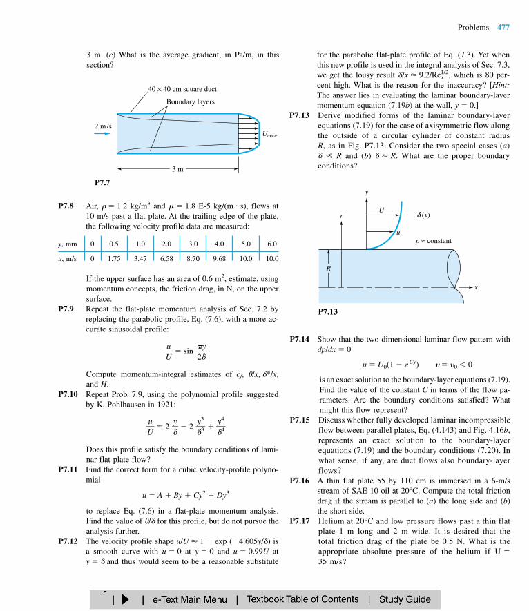
3 m. (c) What is the average gradient, in Pa/m, in this section?

Problems 477

for the parabolic flat-plate profile of Eq. (7.3). Yet whenthis new profile is used in the integral analysis of Sec. 7.3,we get the lousy result /x 9.2/Rex

1/2, which is 80 per-cent high. What is the reason for the inaccuracy? [Hint:The answer lies in evaluating the laminar boundary-layermomentum equation (7.19b) at the wall, y 0.]

P7.13 Derive modified forms of the laminar boundary-layerequations (7.19) for the case of axisymmetric flow alongthe outside of a circular cylinder of constant radius R, as in Fig. P7.13. Consider the two special cases (a) R and (b) R. What are the proper boundary conditions?

2 m /s

3 m

40 × 40 cm square duct

Boundary layers

Ucore

P7.7

P7.8 Air, 1.2 kg/m3 and 1.8 E-5 kg/(m s), flows at10 m/s past a flat plate. At the trailing edge of the plate,the following velocity profile data are measured:

y, mm 0 0.5 1.0 2.0 3.0 4.0 5.0 6.0

u, m/s 0 1.75 3.47 6.58 8.70 9.68 10.0 10.0

If the upper surface has an area of 0.6 m2, estimate, usingmomentum concepts, the friction drag, in N, on the uppersurface.

P7.9 Repeat the flat-plate momentum analysis of Sec. 7.2 byreplacing the parabolic profile, Eq. (7.6), with a more ac-curate sinusoidal profile:

Uu

sin

2

y

Compute momentum-integral estimates of cf, /x, */x,and H.

P7.10 Repeat Prob. 7.9, using the polynomial profile suggestedby K. Pohlhausen in 1921:

Uu

2

y 2

y3

3

y4

4

Does this profile satisfy the boundary conditions of lami-nar flat-plate flow?

P7.11 Find the correct form for a cubic velocity-profile polyno-mial

u A By Cy2 Dy3

to replace Eq. (7.6) in a flat-plate momentum analysis.Find the value of / for this profile, but do not pursue theanalysis further.

P7.12 The velocity profile shape u/U 1 exp (4.605y/) isa smooth curve with u 0 at y 0 and u 0.99U aty and thus would seem to be a reasonable substitute

δ (x)

x

y

r

up ≈ constant

R

U

P7.13

P7.14 Show that the two-dimensional laminar-flow pattern withdp/dx 0

u U0(1 eCy) 0 0

is an exact solution to the boundary-layer equations (7.19).Find the value of the constant C in terms of the flow pa-rameters. Are the boundary conditions satisfied? Whatmight this flow represent?

P7.15 Discuss whether fully developed laminar incompressibleflow between parallel plates, Eq. (4.143) and Fig. 4.16b,represents an exact solution to the boundary-layerequations (7.19) and the boundary conditions (7.20). Inwhat sense, if any, are duct flows also boundary-layerflows?

P7.16 A thin flat plate 55 by 110 cm is immersed in a 6-m/sstream of SAE 10 oil at 20°C. Compute the total frictiondrag if the stream is parallel to (a) the long side and (b)the short side.

P7.17 Helium at 20°C and low pressure flows past a thin flatplate 1 m long and 2 m wide. It is desired that the total friction drag of the plate be 0.5 N. What is theappropriate absolute pressure of the helium if U 35 m/s?

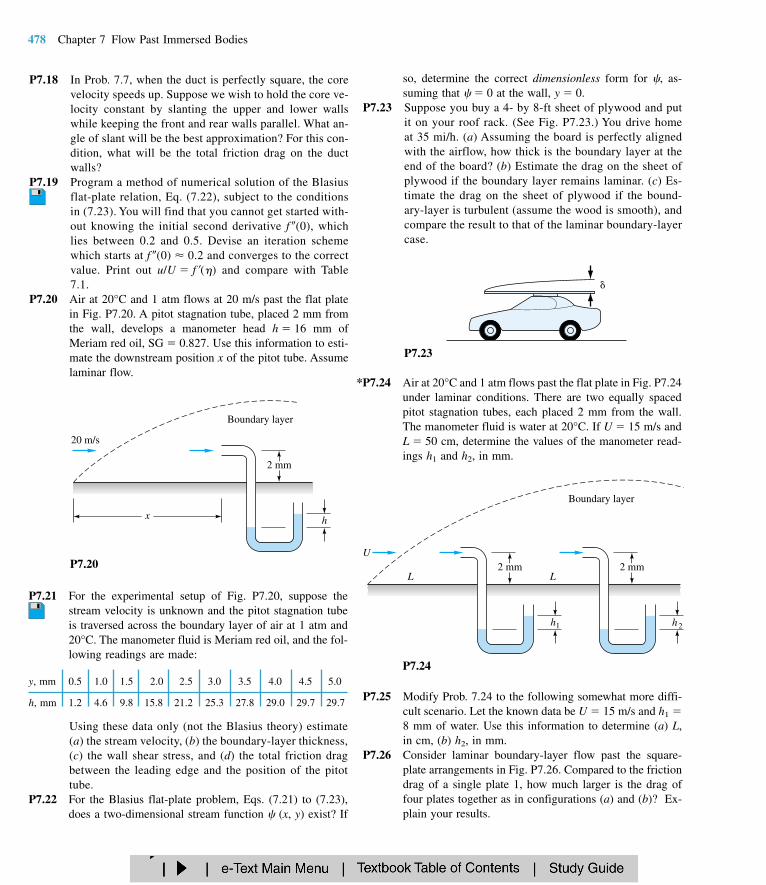
P7.21 For the experimental setup of Fig. P7.20, suppose thestream velocity is unknown and the pitot stagnation tubeis traversed across the boundary layer of air at 1 atm and20°C. The manometer fluid is Meriam red oil, and the fol-lowing readings are made:

y, mm 0.5 1.0 1.5 2.0 2.5 3.0 3.5 4.0 4.5 5.0

h, mm 1.2 4.6 9.8 15.8 21.2 25.3 27.8 29.0 29.7 29.7

Using these data only (not the Blasius theory) estimate(a) the stream velocity, (b) the boundary-layer thickness,(c) the wall shear stress, and (d) the total friction dragbetween the leading edge and the position of the pitottube.

P7.22 For the Blasius flat-plate problem, Eqs. (7.21) to (7.23),does a two-dimensional stream function " (x, y) exist? If

*P7.24 Air at 20°C and 1 atm flows past the flat plate in Fig. P7.24under laminar conditions. There are two equally spacedpitot stagnation tubes, each placed 2 mm from the wall.The manometer fluid is water at 20°C. If U 15 m/s andL 50 cm, determine the values of the manometer read-ings h1 and h2, in mm.

P7.18 In Prob. 7.7, when the duct is perfectly square, the corevelocity speeds up. Suppose we wish to hold the core ve-locity constant by slanting the upper and lower wallswhile keeping the front and rear walls parallel. What an-gle of slant will be the best approximation? For this con-dition, what will be the total friction drag on the ductwalls?

P7.19 Program a method of numerical solution of the Blasiusflat-plate relation, Eq. (7.22), subject to the conditionsin (7.23). You will find that you cannot get started with-out knowing the initial second derivative f (0), whichlies between 0.2 and 0.5. Devise an iteration schemewhich starts at f (0) 0.2 and converges to the correctvalue. Print out u/U f() and compare with Table7.1.

P7.20 Air at 20°C and 1 atm flows at 20 m/s past the flat platein Fig. P7.20. A pitot stagnation tube, placed 2 mm fromthe wall, develops a manometer head h 16 mm ofMeriam red oil, SG 0.827. Use this information to esti-mate the downstream position x of the pitot tube. Assumelaminar flow.

so, determine the correct dimensionless form for ", as-suming that " 0 at the wall, y 0.

P7.23 Suppose you buy a 4- by 8-ft sheet of plywood and putit on your roof rack. (See Fig. P7.23.) You drive homeat 35 mi/h. (a) Assuming the board is perfectly alignedwith the airflow, how thick is the boundary layer at theend of the board? (b) Estimate the drag on the sheet ofplywood if the boundary layer remains laminar. (c) Es-timate the drag on the sheet of plywood if the bound-ary-layer is turbulent (assume the wood is smooth), andcompare the result to that of the laminar boundary-layercase.


h

20 m/s

Boundary layer

2 mm

x

P7.20

P7.23

U

Boundary layer

h2

2 mm

h1

2 mmL L

P7.24

P7.25 Modify Prob. 7.24 to the following somewhat more diffi-cult scenario. Let the known data be U 15 m/s and h1 8 mm of water. Use this information to determine (a) L,in cm, (b) h2, in mm.

P7.26 Consider laminar boundary-layer flow past the square-plate arrangements in Fig. P7.26. Compared to the frictiondrag of a single plate 1, how much larger is the drag offour plates together as in configurations (a) and (b)? Ex-plain your results.

*P7.27 A thin smooth disk of diameter D is immersed parallel toa uniform stream of velocity U. Assuming laminar flowand using flat-plate theory as a guide, develop an approx-imate formula for the drag of the disk.

P7.28 Flow straighteners are arrays of narrow ducts placed inwind tunnels to remove swirl and other in-plane secondaryvelocities. They can be idealized as square boxes con-structed by vertical and horizontal plates, as in Fig. P7.28.The cross section is a by a, and the box length is L. As-suming laminar flat-plate flow and an array of N Nboxes, derive a formula for (a) the total drag on the bun-dle of boxes and (b) the effective pressure drop across thebundle.

Problems 479

P7.29 Let the flow straighteners in Fig. P7.28 form an arrayof 20 20 boxes of size a 4 cm and L 25 cm. Ifthe approach velocity is U0 12 m/s and the fluid issea-level standard air, estimate (a) the total array dragand (b) the pressure drop across the array. Compare withSec. 6.6.

P7.30 Repeat Prob. 7.16 if the fluid is water at 20°C and the platesurface is smooth.

P7.31 Repeat Prob. 7.16 if the fluid is water at 20°C and the platehas an average roughness height of 1.5 mm.

P7.32 A flat plate of length L and height is placed at a walland is parallel to an approaching boundary layer, as in Fig.P7.32. Assume that the flow over the plate is fully turbu-lent and that the approaching flow is a one-seventh-powerlaw

u(y) U0

y

1/7

Using strip theory, derive a formula for the drag coeffi-cient of this plate. Compare this result with the drag of thesame plate immersed in a uniform stream U0.

1 3

2 4

1

(a)P7.26 (b)

1 2 3 4

a

a

L

U0

P7.28

P7.33 An alternate analysis of turbulent flat-plate flow was givenby Prandtl in 1927, using a wall shear-stress formula frompipe flow

w 0.0225U2U

1/4

Show that this formula can be combined with Eqs. (7.33)and (7.40) to derive the following relations for turbulentflat-plate flow:

x cf CD

These formulas are limited to Rex between 5 105 and107.

*P7.34 A thin equilateral-triangle plate is immersed parallel to a12 m/s stream of water at 20°C, as in Fig. P7.34. Assum-ing Retr 5 105, estimate the drag of this plate.

P7.35 The solutions to Prob. 7.26 are (a) F 2.83F1-plate and (b)F 2.0F1-plate. Do not reveal these results to your friends.Repeat Prob. 7.26 assuming the boundary-layer flow is tur-bulent, and comment on the striking increase in numericalvalues.

0.072ReL

1/50.0577Rex

1/50.37Rex

1/5

y

x

UL

δ

δy =

u( y)

P7.32

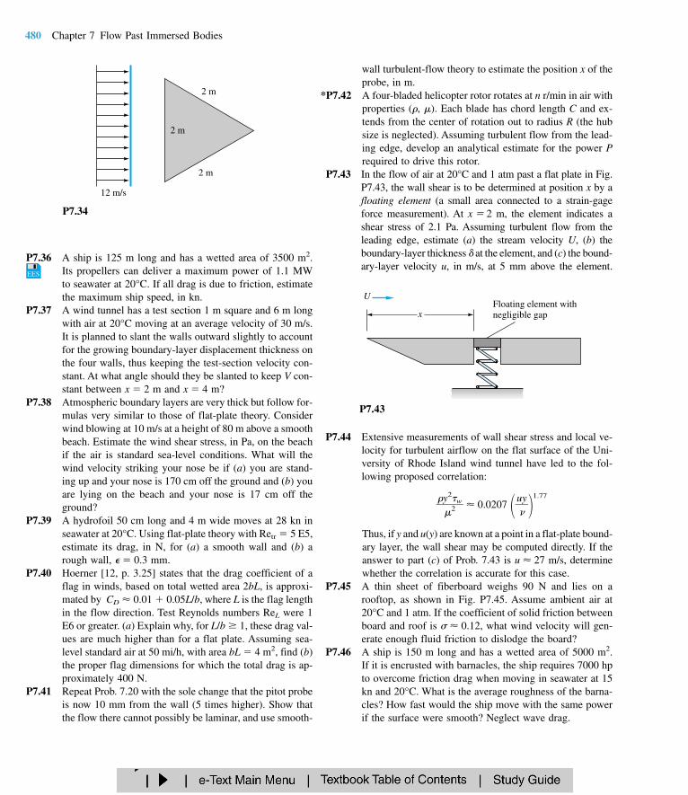
wall turbulent-flow theory to estimate the position x of theprobe, in m.

*P7.42 A four-bladed helicopter rotor rotates at n r/min in air withproperties (, ). Each blade has chord length C and ex-tends from the center of rotation out to radius R (the hubsize is neglected). Assuming turbulent flow from the lead-ing edge, develop an analytical estimate for the power Prequired to drive this rotor.

P7.43 In the flow of air at 20°C and 1 atm past a flat plate in Fig.P7.43, the wall shear is to be determined at position x by afloating element (a small area connected to a strain-gageforce measurement). At x 2 m, the element indicates ashear stress of 2.1 Pa. Assuming turbulent flow from theleading edge, estimate (a) the stream velocity U, (b) theboundary-layer thickness at the element, and (c) the bound-ary-layer velocity u, in m/s, at 5 mm above the element.

P7.36 A ship is 125 m long and has a wetted area of 3500 m2.Its propellers can deliver a maximum power of 1.1 MWto seawater at 20°C. If all drag is due to friction, estimatethe maximum ship speed, in kn.

P7.37 A wind tunnel has a test section 1 m square and 6 m longwith air at 20°C moving at an average velocity of 30 m/s.It is planned to slant the walls outward slightly to accountfor the growing boundary-layer displacement thickness onthe four walls, thus keeping the test-section velocity con-stant. At what angle should they be slanted to keep V con-stant between x 2 m and x 4 m?

P7.38 Atmospheric boundary layers are very thick but follow for-mulas very similar to those of flat-plate theory. Considerwind blowing at 10 m/s at a height of 80 m above a smoothbeach. Estimate the wind shear stress, in Pa, on the beachif the air is standard sea-level conditions. What will thewind velocity striking your nose be if (a) you are stand-ing up and your nose is 170 cm off the ground and (b) youare lying on the beach and your nose is 17 cm off theground?

P7.39 A hydrofoil 50 cm long and 4 m wide moves at 28 kn inseawater at 20°C. Using flat-plate theory with Retr 5 E5,estimate its drag, in N, for (a) a smooth wall and (b) arough wall, 0.3 mm.

P7.40 Hoerner [12, p. 3.25] states that the drag coefficient of aflag in winds, based on total wetted area 2bL, is approxi-mated by CD 0.01 0.05L/b, where L is the flag lengthin the flow direction. Test Reynolds numbers ReL were 1E6 or greater. (a) Explain why, for L/b 1, these drag val-ues are much higher than for a flat plate. Assuming sea-level standard air at 50 mi/h, with area bL 4 m2, find (b)the proper flag dimensions for which the total drag is ap-proximately 400 N.

P7.41 Repeat Prob. 7.20 with the sole change that the pitot probeis now 10 mm from the wall (5 times higher). Show thatthe flow there cannot possibly be laminar, and use smooth-


2 m

2 m

2 m

12 m/s

P7.34

x

UFloating element withnegligible gap

P7.43

P7.44 Extensive measurements of wall shear stress and local ve-locity for turbulent airflow on the flat surface of the Uni-versity of Rhode Island wind tunnel have led to the fol-lowing proposed correlation:

y

2

2w 0.0207

u

y

1.77

Thus, if y and u(y) are known at a point in a flat-plate bound-ary layer, the wall shear may be computed directly. If theanswer to part (c) of Prob. 7.43 is u 27 m/s, determinewhether the correlation is accurate for this case.

P7.45 A thin sheet of fiberboard weighs 90 N and lies on arooftop, as shown in Fig. P7.45. Assume ambient air at20°C and 1 atm. If the coefficient of solid friction betweenboard and roof is # 0.12, what wind velocity will gen-erate enough fluid friction to dislodge the board?

P7.46 A ship is 150 m long and has a wetted area of 5000 m2.If it is encrusted with barnacles, the ship requires 7000 hpto overcome friction drag when moving in seawater at 15kn and 20°C. What is the average roughness of the barna-cles? How fast would the ship move with the same powerif the surface were smooth? Neglect wave drag.

EES

thin, show that the core velocity U(x) in the diffuser isgiven approximately by

U 1 (2x

Ut0

an )/W

where W is the inlet height. Use this velocity distributionwith Thwaites’ method to compute the wall angle forwhich laminar separation will occur in the exit plane whendiffuser length L 2W. Note that the result is indepen-dent of the Reynolds number.

Problems 481

Fiberboard

Roof

2 m 3 m 1 m

1.5 m

2 mU

P7.47 As a case similar to Example 7.5, Howarth also proposedthe adverse-gradient velocity distribution U U0(1 x2/L2) and computed separation at xsep/L 0.271 by a se-ries-expansion method. Compute separation by Thwaites’method and compare.

P7.48 In 1957 H. Görtler proposed the adverse-gradient test cases

U (1

Ux0

/L)n

and computed separation for laminar flow at n 1 to bexsep/L 0.159. Compare with Thwaites’ method, assum-ing 0 0.

P7.49 Based strictly upon your understanding of flat-plate the-ory plus adverse and favorable pressure gradients, explainthe direction (left or right) for which airflow past the slen-der airfoil shape in Fig. P7.49 will have lower total (fric-tion pressure) drag.

P7.45

U ? U ?

P7.49

*P7.50 For flow past a cylinder of radius R as in Fig. P7.50, thetheoretical inviscid velocity distribution along the surfaceis U 2U0 sin (x/R), where U0 is the oncoming streamvelocity and x is the arc length measured from the nose(Chap. 8). Compute the laminar separation point xsep andsep by Thwaites’ method, and compare with the digital-computer solution xsep/R 1.823 (sep 104.5°) given byR. M. Terrill in 1960.

P7.51 Consider the flat-walled diffuser in Fig. P7.51, which issimilar to that of Fig. 6.26a with constant width b. If x ismeasured from the inlet and the wall boundary layers are

RU0

θx

xsep, θsep

P7.50

L

U0 x U(x)

θ

θ

Constant width b

W

P7.51

*P7.52 In Fig. P7.52 a slanted upper wall creates a favorable pres-sure gradient on the upper surface of the flat plate. UseThwaites’ theory to estimate

CD F

12

U20bL

P7.52

Flat plate

Slantedwall

U0h0 x L , b

U(x)12 h0

on the upper plate surface if U0 L/ 105. Compare withEq. (7.27).

P7.53 From Table 7.2, the drag coefficient of a wide plate nor-mal to a stream is approximately 2.0. Let the stream con-ditions be U and p. If the average pressure on the frontof the plate is approximately equal to the free-streamstagnation pressure, what is the average pressure on therear?

P7.54 A chimney at sea level is 2 m in diameter and 40 m high.When it is subjected to 50 mi/h storm winds, what is theestimated wind-induced bending moment about the bot-tom of the chimney?

P7.55 A ship tows a submerged cylinder, which is 1.5 m in di-ameter and 22 m long, at 5 m/s in fresh water at 20°C. Es-timate the towing power, in kW, required if the cylinder is(a) parallel and (b) normal to the tow direction.

P7.56 A delivery vehicle carries a long sign on top, as in Fig.P7.56. If the sign is very thin and the vehicle moves at 55mi/h, estimate the force on the sign (a) with no crosswindand (b) with a 10 mi/h crosswind.

how fast can Joe ride into the head wind? (c) Why is theresult not simply 10 5.0 5.0 m/s, as one might firstsuspect?

P7.60 A fishnet consists of 1-mm-diameter strings overlappedand knotted to form 1- by 1-cm squares. Estimate the dragof 1 m2 of such a net when towed normal to its plane at 3m/s in 20°C seawater. What horsepower is required to tow400 ft2 of this net?

P7.61 A filter may be idealized as an array of cylindrical fibersnormal to the flow, as in Fig. P7.61. Assuming that thefibers are uniformly distributed and have drag coeffi-cients given by Fig. 7.16a, derive an approximate ex-pression for the pressure drop !p through a filter of thick-ness L.


P7.57 The main cross-cable between towers of a coastal suspen-sion bridge is 60 cm in diameter and 90 m long. Estimatethe total drag force on this cable in crosswinds of 50 mi/h.Are these laminar-flow conditions?

P7.58 A long cylinder of rectangular cross section, 5 cm highand 30 cm long, is immersed in water at 20°C flowingat 12 m/s parallel to the long side of the rectangle. Es-timate the drag force on the cylinder, per unit length, ifthe rectangle (a) has a flat face or (b) has a roundednose.

P7.59 Joe can pedal his bike at 10 m/s on a straight level roadwith no wind. The rolling resistance of his bike is 0.80N s/m, i.e., 0.80 N of force per m/s of speed. The dragarea (CDA) of Joe and his bike is 0.422 m2. Joe’s massis 80 kg and that of the bike is 15 kg. He now encoun-ters a head wind of 5.0 m/s. (a) Develop an equation forthe speed at which Joe can pedal into the wind. [Hint: Acubic equation for V will result.] (b) Solve for V, i.e.,

60 cm

8 m

Phil's Pizza: 555-5748

P7.56 P7.62 A sea-level smokestack is 52 m high and has a square cross

section. Its supports can withstand a maximum side forceof 90 kN. If the stack is to survive 90-mi/h hurricane winds,what is its maximum possible width?

P7.63 The cross section of a cylinder is shown in Fig. P7.63. As-sume that on the front surface the velocity is given by po-tential theory (Sec. 8.4), V 2U sin , from which thesurface pressure is computed by Bernoulli’s equation. In

R

Separated-flow wakeθ

V = 2 U∞ sin θ

p∞ , U∞

P7.63

Filter section

U

p + ∆ pUp

Array ofcylinders(fibers)

P7.61

the separated flow on the rear, the pressure is assumedequal to its value at 90°. Compute the theoretical dragcoefficient and compare with Table 7.2.

P7.64 A parachutist jumps from a plane, using an 8.5-m-diameter chute in the standard atmosphere. The total massof the chutist and the chute is 90 kg. Assuming an openchute and quasi-steady motion, estimate the time to fallfrom 2000- to 1000-m altitude.

P7.65 The drag of a sphere at very low Reynolds numbers ReD 1 was given analytically by G. G. Stokes in 1851:F 3 VD [2, pp. 175–178]. This formula is an exam-ple of Stokes’ law of creeping motion, where inertia is neg-ligible. Show that the drag coefficient in this region isCD 24/ReD. A 1-mm-diameter sphere falls in 20°C glycerin at 2.5 mm/s. Is this a creeping motion? Compute(a) the Reynolds number, (b) the drag, and (c) the specificgravity of the sphere.

P7.66 A sphere of density s and diameter D is dropped fromrest in a fluid of density and viscosity . Assuming aconstant drag coefficient Cd 0

, derive a differential equa-tion for the fall velocity V(t) and show that the solutionis

V 1/2

tanh Ct

C 1/2

where S s / is the specific gravity of the sphere mate-rial.

P7.67 Apply the theory of Prob. 7.66 to a steel sphere of diam-eter 2 cm, dropped from rest in water at 20°C. Estimatethe time required for the sphere to reach 99 percent of itsterminal (zero-acceleration) velocity.

P7.68 A baseball weighs 145 g and is 7.35 cm in diameter. It isdropped from rest from a 35-m-high tower at approxi-mately sea level. Assuming a laminar-flow drag coeffi-cient, estimate (a) its terminal velocity and (b) whether itwill reach 99 percent of its terminal velocity before it hitsthe ground.

P7.69 Two baseballs from Prob. 7.68 are connected to a rod 7mm in diameter and 56 cm long, as in Fig. P7.69. Whatpower, in W, is required to keep the system spinning at400 r/min? Include the drag of the rod, and assume sea-level standard air.

P7.70 A baseball from Prob. 7.68 is batted upward during a gameat an angle of 45° and an initial velocity of 98 mi/h. Ne-glect spin and lift. Estimate the horizontal distance trav-eled, (a) neglecting drag and (b) accounting for drag in anumerical (computer) solution with a transition Reynoldsnumber ReD,crit 2.5 E5.

3gCd 0(S 1)

4S2D

4gD(S 1)

3Cd 0

Problems 483

P7.71 A football weighs 0.91 lbf and approximates an ellipsoid6 in in diameter and 12 in long (Table 7.3). It is thrownupward at a 45° angle with an initial velocity of 80 ft/s.Neglect spin and lift. Assuming turbulent flow, estimatethe horizontal distance traveled, (a) neglecting drag and(b) accounting for drag with a numerical (computer)model.

P7.72 A settling tank for a municipal water supply is 2.5 m deep,and 20°C water flows through continuously at 35 cm/s.Estimate the minimum length of the tank which will ensure that all sediment (SG 2.55) will fall to the bot-tom for particle diameters greater than (a) 1 mm and (b) 100 m.

P7.73 A balloon is 4 m in diameter and contains helium at 125kPa and 15°C. Balloon material and payload weigh 200N, not including the helium. Estimate (a) the terminal as-cent velocity in sea-level standard air, (b) the final stan-dard altitude (neglecting winds) at which the balloon willcome to rest, and (c) the minimum diameter (4 m) forwhich the balloon will just barely begin to rise in sea-levelstandard air.

P7.74 If D 4 m in Prob. 7.73 and the helium remains at15°C and 125 kPa, estimate the time required for theballoon to rise through the standard atmosphere fromsea level to its equilibrium altitude, which is approxi-mately 4000 m.

P7.75 The helium-filled balloon in Fig. P7.75 is tethered at 20°Cand 1 atm with a string of negligible weight and drag. Thediameter is 50 cm, and the balloon material weighs 0.2 N,

28 cm

Ω

Baseball 28 cm

Baseball

P7.69

D = 50 cm

θU

P7.75

EES

not including the helium. The helium pressure is 120 kPa.Estimate the tilt angle if the airstream velocity U is (a)5 m/s or (b) 20 m/s.

P7.76 Extend Prob. 7.75 to make a smooth plot of tilt angle versus stream velocity U in the range 1 U 12 mi/h.(A spreadsheet is recommended for this task.) Commenton the effectiveness of this system as an air-velocity in-strument.

P7.77 Modify Prob. 7.75 as follows: Let the fluid be water at20°C, and let the 50-cm-diameter sphere be solid cork(SG 0.16). Estimate the tilt angle if the water veloc-ity U is 3 m/s.

P7.78 Apply Prob. 7.61 to a filter consisting of 300- m-diameter fibers packed 250 per square centimeter in theplane of Fig. P7.61. For air at 20°C and 1 atm flowing at1.5 m/s, estimate the pressure drop if the filter is 5 cmthick.

P7.79 Assume that a radioactive dust particle approximates asphere of density 2400 kg/m3. How long, in days, will it take such a particle to settle to sea level from an alti-tude of 12 km if the particle diameter is (a) 1 m or (b) 20 m?

P7.80 A heavy sphere attached to a string should hang at anangle when immersed in a stream of velocity U, as inFig. P7.80. Derive an expression for as a function ofthe sphere and flow properties. What is if the sphereis steel (SG 7.86) of diameter 3 cm and the flow issea-level standard air at U 40 m/s? Neglect the stringdrag.

1.2 ft2 falling feet first [12, p. 313]. What are the mini-mum and maximum terminal speeds that can be achievedby a skydiver at 5000-ft standard altitude?

P7.83 A high-speed car has a drag coefficient of 0.3 and a frontalarea of 1 m2. A parachute is to be used to slow this carfrom 80 to 40 m/s in 8 s. What should the chute diameterbe? What distance will be traveled during this decelera-tion? Take m 2000 kg.

P7.84 A Ping-Pong ball weighs 2.6 g and has a diameter of 3.8cm. It can be supported by an air jet from a vacuum cleaneroutlet, as in Fig. P7.84. For sea-level standard air, what jetvelocity is required?


P7.81 A typical U.S. Army parachute has a projected diame-ter of 28 ft. For a payload mass of 80 kg, (a) what ter-minal velocity will result at 1000-m standard altitude?For the same velocity and net payload, what size drag-producing “chute” is required if one uses a square flatplate held (b) vertically and (c) horizontally? (Neglectthe fact that flat shapes are not dynamically stable infree fall.)

P7.82 The average skydiver with parachute unopened weighs 175lbf and has a drag area CD A 9 ft2 spread-eagled and

*P7.85 An aluminum cylinder (SG 2.7) slides concentricallydown a taut 1-mm-diameter wire as shown in Fig. P7.85.Its length L 8 cm, and its radius R 1 cm. A 2-mm-di-ameter hole down the cylinder center is lubricated by SAE30 oil at 20°C. Estimate the terminal fall velocity V of thecylinder if ambient air drag is (a) neglected and (b) in-cluded. Assume air at 1 atm and 20°C.

θ

D, ρs

U

P7.80

P7.84

P7.85

Oil film

V

R

L

P7.86 Hoerner [Ref. 12, pp. 3–25] states that the drag coefficientof a flag of 21 aspect ratio is 0.11 based on planformarea. The University of Rhode Island has an aluminumflagpole 25 m high and 14 cm in diameter. It flies equal-sized national and state flags together. If the fracture stressof aluminum is 210 MPa, what is the maximum flag sizethat can be used yet avoids breaking the flagpole in hur-ricane (75 mi/h) winds?

P7.87 A tractor-trailer truck has a drag-area CD A 8 m2 bareand 6.7 m2 with an aerodynamic deflector (Fig. 7.18b). Itsrolling resistance is 50 N for each mile per hour of speed.Calculate the total horsepower required at sea level withand without the deflector if the truck moves at (a) 55 mi/hand (b) 75 mi/h.

P7.88 A pickup truck has a clean drag-area CD A of 35 ft2. Es-timate the horsepower required to drive the truck at 55mi/h (a) clean and (b) with the 3- by 6-ft sign in Fig.P7.88 installed if the rolling resistance is 150 lbf at sealevel.

torque of 0.004 N m. Making simplifying assumptionsto average out the time-varying geometry, estimate andplot the variation of anemometer rotation rate $ with windvelocity U in the range 0 U 25 m/s for sea-level stan-dard air.

Problems 485

P7.89 A water tower is approximated by a 15-m-diameter spheremounted on a 1-m-diameter rod 20 m long. Estimate thebending moment at the root of the rod due to aerodynamicforces during hurricane winds of 40 m/s.

P7.90 In the great hurricane of 1938, winds of 85 mi/h blew overa boxcar in Providence, Rhode Island. The boxcar was 10ft high, 40 ft long, and 6 ft wide, with a 3-ft clearanceabove tracks 4.8 ft apart. What wind speed would topplea boxcar weighing 40,000 lbf?

*P7.91 A cup anemometer uses two 5-cm-diameter hollow hemi-spheres connected to 15-cm rods, as in Fig. P7.91. Roddrag is negligible, and the central bearing has a retarding

P7.92 A 1500-kg automobile uses its drag area CD A 0.4 m2,plus brakes and a parachute, to slow down from 50 m/s.Its brakes apply 5000 N of resistance. Assume sea-levelstandard air. If the automobile must stop in 8 s, what di-ameter parachute is appropriate?

P7.93 A hot-film probe is mounted on a cone-and-rod system ina sea-level airstream of 45 m/s, as in Fig. P7.93. Estimatethe maximum cone vertex angle allowable if the flow-in-duced bending moment at the root of the rod is not to ex-ceed 30 N cm.

Eat atJoe's

6 ft

3 ft

P7.88

D = 5 cm

Ω

D = 5 cm

U

15 cm

15 cm

P7.91

Ho t film

20 cm

3 cm

5-mmdia.

45 m/s

P7.93 EES

P7.94 A rotary mixer consists of two 1-m-long half-tubes rotat-ing around a central arm, as in Fig. P7.94. Using the dragfrom Table 7.2, derive an expression for the torque T re-quired to drive the mixer at angular velocity $ in a fluid

of density . Suppose that the fluid is water at 20°C andthe maximum driving power available is 20 kW. What isthe maximum rotation speed $ r/min?

mobile of mass 1500 kg and frontal area 2 m2, the fol-lowing velocity-versus-time data are obtained during acoastdown:

t, s 0 10 20 30 40

V, m/s 27.0 24.2 21.8 19.7 17.9

Estimate (a) the rolling resistance and (b) the drag coef-ficient. This problem is well suited for digital-computeranalysis but can be done by hand also.

*P7.98 A buoyant ball of specific gravity SG 1 dropped intowater at inlet velocity V0 will penetrate a distance h andthen pop out again, as in Fig. P7.98. Make a dynamicanalysis of this problem, assuming a constant drag coef-ficient, and derive an expression for h as a function ofthe system properties. How far will a 5-cm-diameter ballwith SG 0.5 and CD 0.47 penetrate if it enters at 10 m/s?


P7.99 Two steel balls (SG 7.86) are connected by a thin hingedrod of negligible weight and drag, as in Fig. P7.99. A stopprevents the rod from rotating counterclockwise. Estimatethe sea-level air velocity U for which the rod will first be-gin to rotate clockwise.

P7.94

D = 5 cm

Ω

R = 1 m

h

V0

DiameterD

(SG < 1)

P7.98

D = 1 cm

D = 2 cm

U Stop

10 cm

10 cm

Hinge

45˚

P7.99

P7.95 An airplane weighing 12 kN, with a drag-area CD A 5 m2, lands at sea level at 55 m/s and deploys a drag para-chute 3 m in diameter. No other brakes are applied. (a) How long will it take the plane to slow down to 30 m/s? (b) How far will it have traveled in that time?

*P7.96 A Savonius rotor (Fig. 6.29b) can be approximated bythe two open half-tubes in Fig. P7.96 mounted on a cen-tral axis. If the drag of each tube is similar to that inTable 7.2, derive an approximate formula for the rota-tion rate $ as a function of U, D, L, and the fluid prop-erties (, ).

Axis

U

L

L

D

D

Ω

P7.96

P7.97 A simple measurement of automobile drag can be foundby an unpowered coastdown on a level road with nowind. Assume constant rolling resistance. For an auto-

P7.100 In creeping motion or Stokes’ flow at velocity U past asphere of diameter D, density (fluid inertia) is unim-portant and the drag force is F 3 UD. This formulais valid if ReD 1.0 (see Fig. 7.16b). (a) Verify thatStokes’ formula is equivalent to CD 24/ReD. (b) De-termine the largest diameter raindrop whose terminal fallvelocity follows Stokes’ formula in sea-level standardair.

P7.101 Icebergs can be driven at substantial speeds by the wind.Let the iceberg be idealized as a large, flat cylinder,D % L, with one-eighth of its bulk exposed, as in Fig.P7.101. Let the seawater be at rest. If the upper andlower drag forces depend upon relative velocities be-tween the iceberg and the fluid, derive an approximateexpression for the steady iceberg speed V when drivenby wind velocity U.

Problems 487

P7.102 Sand particles (SG 2.7), approximately spherical withdiameters from 100 to 250 m, are introduced into an up-ward-flowing stream of water at 20°C. What is the mini-mum water velocity which will carry all the sand particlesupward?

P7.103 When immersed in a uniform stream V, a heavy rodhinged at A will hang at Pode’s angle , after an analysisby L. Pode in 1951 (Fig. P7.103). Assume that the cylin-der has normal drag coefficient CDN and tangential coef-ficient CDT which relate the drag forces to VN and VT, re-spectively. Derive an expression for Pode’s angle as afunction of the flow and rod parameters. Find for a steelrod, L 40 cm, D 1 cm, hanging in sea-level air atV 35 m/s.

P7.104 Suppose that the body in Fig. P7.103 is a thin plateweighing 0.6 N, of length L 20 cm and width b 4cm into the paper. For sea-level standard air, plot Pode’sangle versus velocity V in the range 0 V 40 m/s.Would this device make a good air-velocity meter(anemometer)?

P7.105 A ship 50 m long, with a wetted area of 800 m2, has thehull shape tested in Fig. 7.19. There are no bow or sternbulbs. The total propulsive power available is 1 MW. Forseawater at 20°C, plot the ship’s velocity V kn versuspower P for 0 P 1 MW. What is the most efficientsetting?

P7.106 A smooth steel 1-cm-diameter sphere (W 0.04 N) isfired vertically at sea level at the initial supersonic veloc-ity V0 1000 m/s. Its drag coefficient is given by Fig.7.20. Assuming that the speed of sound is constant at a 343 m/s, compute the maximum altitude of the projectile(a) by a simple analytical estimate and (b) by a digital-computer program.

P7.107 Repeat Prob. 7.106 if the body is a 9-mm steel bullet (W 0.07 N) which approximates the “pointed body of revolu-tion” in Fig. 7.20.

P7.108 The data in Fig. P7.108 are for the lift and drag of a spin-ning sphere from Ref. 12, pp. 7–20. Suppose that a tennisball (W 0.56 N, D 6.35 cm) is struck at sea level withinitial velocity V0 30 m/s and “topspin” (front of the ballrotating downward) of 120 r/s. If the initial height of theball is 1.5 m, estimate the horizontal distance traveled be-fore it strikes the ground.

P7.109 Repeat Prob. 7.108 if the ball is struck with “underspin”(front of the ball rotating upward).

P7.110 A baseball pitcher throws a curveball with an initial ve-locity of 65 mi/h and a spin of 6500 r/min about a verti-cal axis. A baseball weighs 0.32 lbf and has a diameter of2.9 in. Using the data of Fig. P7.108 for turbulent flow,estimate how far such a curveball will have deviated fromits straight-line path when it reaches home plate 60.5 ftaway.

*P7.111 A table tennis ball has a mass of 2.6 g and a diameterof 3.81 cm. It is struck horizontally at an initial veloc-ity of 20 m/s while it is 50 cm above the table, as inFig. P7.111. For sea-level air, what spin, in r/min, willcause the ball to strike the opposite edge of the table,4 m away? Make an analytical estimate, using Fig.P7.108, and account for the fact that the ball deceler-ates during flight.

P7.101

U>>D L

L / 8

7L / 8V

Iceberg

P7.103

V

Aθ

L, D, ρs

CD N , VN

CD T , VT

P7.112 Repeat Prob. 7.111 by making a detailed digital-computersolution for the flight path of the ball. Use Fig. P7.108 forlift and drag.

P7.113 An automobile has a mass of 1000 kg and a drag-areaCDA 0.7 m2. The rolling resistance of 70 N is approxi-mately constant. The car is coasting without brakes at 90km/h as it begins to climb a hill of 10 percent grade(slope tan1 0.1 5.71°). How far up the hill will thecar come to a stop?

*P7.114 Suppose that the car in Prob. 7.113 is placed at the top ofthe 10 percent grade hill and released from rest to coastdown without brakes. What will be its speed, in km/h, af-ter dropping a vertical distance of 20 m?

P7.115 An airplane weighs 180 kN and has a wing area of 160m2 and a mean chord of 4 m. The airfoil properties aregiven by Fig. 7.25. If the airplane cruises at 250 mi/h at3000-m standard altitude, what propulsive power is re-quired to overcome wing drag?

P7.116 The airplane of Prob. 7.115 is designed to land at V0 1.2Vstall, using a split flap set at 60°. What is the properlanding speed in mi/h? What power is required for takeoffat the same speed?

P7.117 Suppose that the airplane of Prob. 7.115 takes off at sealevel without benefit of flaps, with CL constant so that thetakeoff speed is 100 mi/h. Estimate the takeoff distance ifthe thrust is 10 kN. How much thrust is needed to makethe takeoff distance 1250 m?

*P7.118 Suppose that the airplane of Prob. 7.115 is fitted with allthe best high-lift devices of Fig. 7.28. What is its mini-mum stall speed in mi/h? Estimate the stopping distanceif the plane lands at V0 1.25Vstall with constant CL 3.0and CD 0.2 and the braking force is 20 percent of theweight on the wheels.

P7.119 An airplane has a mass of 5000 kg, a maximum thrust of7000 N, and a rectangular wing with aspect ratio 6.0. Ittakes off at sea level with a 60° split flap whose two-dimensional properties are shown in Fig. 7.25. Assume all lift and all drag are due to the wing. What is the proper wing size if the takeoff distance is to be 1 km?

P7.120 Show that if Eqs. (7.70) and (7.71) are valid, the maxi-mum lift-to-drag ratio occurs when CD 2CD. What are


P7.111

20 m/s

50 cm

4 m

ω?

?

P7.108

EES

EES

Figure Unavailable

(L/D)max and for a symmetric wing when AR 5 andCD 0.009?

P7.121 In gliding (unpowered) flight, the lift and drag are in equi-librium with the weight. Show that if there is no wind, theaircraft sinks at an angle

tan dlriaftg

For a sailplane of mass 200 kg, wing area 12 m2, and as-pect ratio 11, with an NACA 0009 airfoil, estimate (a) thestall speed, (b) the minimum gliding angle, and (c) themaximum distance it can glide in still air when it is 1200m above level ground.

P7.122 A boat of mass 2500 kg has two hydrofoils, each of chord30 cm and span 1.5 m, with CL,max 1.2 and CD 0.08.Its engine can deliver 130 kW to the water. For seawaterat 20°C, estimate (a) the minimum speed for which the

foils support the boat and (b) the maximum speed attain-able.

P7.123 In prewar days there was a controversy, perhaps apocryphal,about whether the bumblebee has a legitimate aerodynamicright to fly. The average bumblebee (Bombus terrestris)weighs 0.88 g, with a wing span of 1.73 cm and a wing areaof 1.26 cm2. It can indeed fly at 10 m/s. Using fixed-wingtheory, what is the lift coefficient of the bee at this speed? Isthis reasonable for typical airfoils?

*P7.124 The bumblebee can hover at zero speed by flapping itswings. Using the data of Prob. 7.123, devise a theory forflapping wings where the downstroke approximates a shortflat plate normal to the flow (Table 7.3) and the upstrokeis feathered at nearly zero drag. How many flaps per sec-ond of such a model wing are needed to support the bee’sweight? (Actual measurements of bees show a flappingrate of 194 Hz.)

Fundamentals of Engineering Exam Problems 489

Word Problems

W7.1 How do you recognize a boundary layer? Cite some phys-ical properties and some measurements which reveal ap-propriate characteristics.

W7.2 In Chap. 6 the Reynolds number for transition to turbu-lence in pipe flow was about Retr 2300, whereas in flat-plate flow Retr 1 E6, nearly three orders of magnitudehigher. What accounts for the difference?

W7.3 Without writing any equations, give a verbal description ofboundary-layer displacement thickness.

W7.4 Describe, in words only, the basic ideas behind the “bound-ary-layer approximations.”

W7.5 What is an adverse pressure gradient? Give three examplesof flow regimes where such gradients occur.

W7.6 What is a favorable pressure gradient? Give three exam-ples of flow regimes where such gradients occur.

W7.7 The drag of an airfoil (Fig. 7.12) increases considerably ifyou turn the sharp edge around 180° to face the stream.Can you explain this?

W7.8 In Table 7.3, the drag coefficient of a spruce tree decreasessharply with wind velocity. Can you explain this?

W7.9 Thrust is required to propel an airplane at a finite forwardvelocity. Does this imply an energy loss to the system? Ex-plain the concepts of thrust and drag in terms of the firstlaw of thermodynamics.

W7.10 How does the concept of drafting, in automobile and bi-cycle racing, apply to the material studied in this chapter?

W7.11 The circular cylinder of Fig. 7.13 is doubly symmetric andtherefore should have no lift. Yet a lift sensor would defi-nitely reveal a finite root-mean-square value of lift. Canyou explain this behavior?

W7.12 Explain in words why a thrown spinning ball moves in acurved trajectory. Give some physical reasons why a sideforce is developed in addition to the drag.

Fundamentals of Engineering Exam Problems

FE7.1 A smooth 12-cm-diameter sphere is immersed in a streamof 20°C water moving at 6 m/s. The appropriate Reynoldsnumber of this sphere is approximately(a) 2.3 E5, (b) 7.2 E5, (c) 2.3 E6, (d) 7.2 E6, (e) 7.2 E7

FE7.2 If, in Prob. FE7.1, the drag coefficient based upon frontalarea is 0.5, what is the drag force on the sphere?(a) 17 N, (b) 51 N, (c) 102 N, (d) 130 N, (e) 203 N

FE7.3 If, in Prob. FE7.1, the drag coefficient based upon frontalarea is 0.5, at what terminal velocity will an aluminumsphere (SG 2.7) fall in still water?(a) 2.3 m/s, (b) 2.9 m/s, (c) 4.6 m/s, (d) 6.5 m/s, (e) 8.2 m/s

FE7.4 For flow of sea-level standard air at 4 m/s parallel to a thinflat plate, estimate the boundary-layer thickness at x 60cm from the leading edge:(a) 1.0 mm, (b) 2.6 mm, (c) 5.3 mm, (d) 7.5 mm,(e) 20.2 mm

FE7.5 In Prob. FE7.4, for the same flow conditions, what is thewall shear stress at x 60 cm from the leading edge?(a) 0.053 Pa, (b) 0.11 Pa, (c) 0.16 Pa, (d) 0.32 Pa,(e) 0.64 Pa

FE7.6 Wind at 20°C and 1 atm blows at 75 km/h past a flagpole18 m high and 20 cm in diameter. The drag coefficient,

based upon frontal area, is 1.15. Estimate the wind-induced bending moment at the base of the pole.(a) 9.7 kN m, (b) 15.2 kN m, (c) 19.4 kN m,(d) 30.5 kN m, (e) 61.0 kN m

FE7.7 Consider wind at 20°C and 1 atm blowing past a chimney 30m high and 80 cm in diameter. If the chimney may fractureat a base bending moment of 486 kN m, and its drag coef-ficient based upon frontal area is 0.5, what is the approximatemaximum allowable wind velocity to avoid fracture?(a) 50 mi/h, (b) 75 mi/h, (c) 100 mi/h, (d) 125 mi/h,(e) 150 mi/h

FE7.8 A dust particle of density 2600 kg/m3, small enough tosatisfy Stokes’ drag law, settles at 1.5 mm/s in air at 20°Cand 1 atm. What is its approximate diameter?(a) 1.8 m, (b) 2.9 m, (c) 4.4 m, (d) 16.8 m,(e) 234 m

FE7.9 An airplane has a mass of 19,550 kg, a wing span of 20m, and an average wing chord of 3 m. When flying in airof density 0.5 kg/m3, its engines provide a thrust of 12 kNagainst an overall drag coefficient of 0.025. What is itsapproximate velocity?(a) 250 mi/h, (b) 300 mi/h, (c) 350 mi/h, (d) 400 mi/h,(e) 450 mi/h

FE7.10 For the flight conditions of the airplane in Prob. FE7.9above, what is its approximate lift coefficient?(a) 0.1, (b) 0.2, (c) 0.3, (d) 0.4, (e) 0.5


Comprehensive Problems

C7.1 Jane wants to estimate the drag coefficient of herself on herbicycle. She measures the projected frontal area to be 0.40m2 and the rolling resistance to be 0.80 N s/m. The massof the bike is 15 kg, while the mass of Jane is 80 kg. Janecoasts down a long hill which has a constant 4° slope. (SeeFig. C7.1.) She reaches a terminal (steady state) speed of14 m/s down the hill. Estimate the aerodynamic drag coef-ficient CD of the rider and bicycle combination.

C7.2 Air at 20°C and 1 atm flows at Vavg 5 m/s between long,smooth parallel heat-exchanger plates 10 cm apart, as in Fig.C7.2. It is proposed to add a number of widely spaced 1-cm-long interrupter plates to increase the heat transfer, as shown.Although the flow in the channel is turbulent, the boundarylayers over the interrupter plates are essentially laminar. As-sume all plates are 1 m wide into the paper. Find (a) the pres-sure drop in Pa/m without the small plates present. Then find(b) the number of small plates per meter of channel lengthwhich will cause the pressure drop to rise to 10.0 Pa/m.

C7.3 A new pizza store is planning to open. They will, of course,offer free delivery, and therefore need a small delivery carwith a large sign attached. The sign (a flat plate) is 1.5 ft

&

V

C7.1

high and 5 ft long. The boss (having no feel for fluid me-chanics) mounts the sign bluntly facing the wind. One of hisdrivers is taking fluid mechanics and tells his boss he cansave lots of money by mounting the sign parallel to the wind.(See Fig. C7.3.) (a) Calculate the drag (in lbf) on the signalone at 40 mi/h (58.7 ft/s) in both orientations. (b) Supposethe car without any sign has a drag coefficient of 0.4 and afrontal area of 40 ft2. For V 40 mi/h, calculate the totaldrag of the car-sign combination for both orientations. (c) Ifthe car has a rolling resistance of 40 lbf at 40 mi/h, calcu-late the horsepower required by the engine to drive the carat 40 mi/h in both orientations. (d) Finally, if the engine candeliver 10 hp for 1 h on a gallon of gasoline, calculate thefuel efficiency in mi/gal for both orientations at 40 mi/h.

C7.2

Interrupter platesL 1 cmU 5 m/s

Design Project

D7.1 It is desired to design a cup anemometer for wind speed,similar to Fig. P7.91, with a more sophisticated approachthan the “average-torque” method of Prob. 7.91. The designshould achieve an approximately linear relation betweenwind velocity and rotation rate in the range 20 U 40mi/h, and the anemometer should rotate at about 6 r/s atU 30 mi/h. All specifications—cup diameter D, rodlength L, rod diameter d, the bearing type, and all materi-

als—are to be selected through your analysis. Make suit-able assumptions about the instantaneous drag of the cupsand rods at any given angle (t) of the system. Computethe instantaneous torque T(t), and find and integrate the in-stantaneous angular acceleration of the device. Develop acomplete theory for rotation rate versus wind speed in therange 0 U 50 mi/h. Try to include actual commercialbearing-friction properties.

References 491

C7.3

Air

Cup shape

L

m

C7.4

C7.4 Consider a pendulum with an unusual bob shape: a hemi-spherical cup of diameter D whose axis is in the plane ofoscillation, as in Fig. C7.4. Neglect the mass and drag ofthe rod L. (a) Set up the differential equation for the os-cillation (t), including different cup drag (air density )in each direction, and (b) nondimensionalize this equation.(c) Determine the natural frequency of oscillation for small 1 rad. (d) For the special case L 1 m, D 10 cm,m 50 g, and air at 20°C and 1 atm, with (0) 30°, find(numerically) the time required for the oscillation ampli-tude to drop to 1°.

References

1. H. Schlichting, Boundary Layer Theory, 7th ed., McGraw-Hill, New York, 1979.

2. F. M. White, Viscous Fluid Flow, 2d ed., McGraw-Hill, NewYork, 1991.

3. L. Rosenhead (ed.), Laminar Boundary Layers, Oxford Uni-versity Press, London, 1963.

4. D. A. Anderson, J. C. Tannehill, and R. H. Pletcher, Com-putational Fluid Mechanics and Heat Transfer, 2d ed., Hemi-sphere, New York, 1997.

5. R. H. Pletcher and C. L. Dancey, “A Direct Method of Cal-culating through Separated Regions in Boundary LayerFlow,” J. Fluids Eng., September 1976, pp. 568–572.

6. P. K. Chang, Control of Flow Separation, McGraw-Hill, NewYork, 1976. See also P. K. Chang, Recent Development inFlow Separation, Pang Han Pub. Co., Seoul, Korea, 1983.

7. T. von Kármán, “On Laminar and Turbulent Friction,” Z.Angew. Math. Mech., vol. 1, 1921, pp. 235–236.

8. G. B. Schubauer and H. K. Skramstad, “Laminar BoundaryLayer Oscillations and Stability of Laminar Flow,” Natl. Bur.Stand. Res. Pap. 1772, April 1943 (see also J. Aero. Sci., vol.14, 1947, pp. 69–78, and NACA Rep. 909, 1947).

9. W. Rodi, Turbulence Models and Their Application in Hy-draulics, Brookfield Pub., Brookfield, VT, 1984.

10. P. W. Runstadler, Jr., et al., “Diffuser Data Book,” Creare Inc.,Tech. Note 186, Hanover, NH, May 1975.

11. B. Thwaites, “Approximate Calculation of the LaminarBoundary Layer,” Aeronaut. Q., vol. 1, 1949, pp. 245–280.

12. S. F. Hoerner, Fluid Dynamic Drag, published by the author,Midland Park, NJ, 1965.

13. J. D. Anderson, Fundamentals of Aerodynamics, 2d ed., Mc-Graw-Hill, New York, 1991.

14. V. Tucker and G. C. Parrott, “Aerodynamics of Gliding Flightof Falcons and Other Birds,” J. Exp. Biol., vol. 52, 1970, pp.345–368.

15. Eric Tupper, Introduction to Naval Architecture, Butterworth,Boston, 1996.

16. I. H. Abbott and A. E. von Doenhoff, Theory of Wing Sec-tions, Dover, New York, 1959.

17. R. L. Kline and F. F. Fogleman, Airfoil for Aircraft, U.S.Patent 3,706,430 Dec. 19, 1972.

18. T. Y. Yu et al. (eds.), Swimming and Flying in Nature: Pro-ceedings of a Symposium, Plenum, New York, 1975.

19. National Committee for Fluid Mechanics Films, IllustratedExperiments in Fluid Mechanics, M.I.T. Press, Cambridge,MA, 1972.

20. E. M. Uram and H. E. Weber (eds.), “Laminar and TurbulentBoundary Layers,” ASME Symp. Proc., vol. I00167, Febru-ary 1984.

21. G. Sovran, T. Morel, and W. T. Mason, Jr. (eds.), Aerody-namic Drag Mechanisms of Bluff Bodies and Road Vehicles,Plenum, New York, 1978.

22. W. H. Hucho, Aerodynamics of Road Vehicles, Butterworth,Boston, 1986.

23. R. D. Blevins, Applied Fluid Dynamics Handbook, van Nos-trand Reinhold, New York, 1984.

24. R. C. Johnson, Jr., G. E. Ramey, and D. S. O’Hagen, “WindInduced Forces on Trees,” J. Fluids Eng., vol. 104, March1983, pp. 25–30.

25. P. W. Bearman et al., “The Effect of a Moving Floor on Wind-Tunnel Simulation of Road Vehicles,” Paper No. 880245,SAE Transactions, J. Passenger Cars, vol. 97, sec. 4, 1988,pp. 4.200–4.214.

26. CRC Handbook of Tables for Applied Engineering Science,2d ed., CRC Press, Boca Raton, FL, 1973.

27. T. Inui, “Wavemaking Resistance of Ships,” Trans. Soc. Nav.Arch. Marine Engrs., vol. 70, 1962, pp. 283–326.

28. L. Larsson et al., “A Method for Resistance and Flow Pre-diction in Ship Design,” Trans. Soc. Nav. Arch. Marine En-grs., vol. 98, 1990, pp. 495–535.

29. R. L. Street, G. Z. Watters, and J. K. Vennard, ElementaryFluid Mechanics, 7th ed., Wiley, New York, 1995.

30. J. D. Anderson, Jr., Modern Compressible Flow, with His-torical Perspective, 2d ed., McGraw-Hill, New York, 1990.

31. J. D. Anderson, Jr., Hypersonic and High Temperature GasDynamics, McGraw-Hill, New York, 1989.

32. J. Rom, High Angle of Attack Aerodynamics: Subsonic, Tran-sonic, and Supersonic Flows, Springer-Verlag, New York,1992.

33. S. Vogel, “Drag and Reconfiguration of Broad Leaves in HighWinds,” J. Exp. Bot., vol. 40, no. 217, August 1989, pp. 941–948.

34. S. Vogel, Life in Moving Fluids, Princeton University Press,Princeton, NJ, 1981.

35. J. A. C. Humphrey (ed.), Proceedings 1st InternationalSymposium on Mechanics of Plants, Animals, and TheirEnvironment, Engineering Foundation, New York, January1998.

36. D. D. Joseph, R. Bai, K. P. Chen, and Y. Y. Renardy, “Core-Annular Flows,” Annu. Rev. Fluid Mech., vol. 29, 1997, pp.65–90.

37. J. W. Hoyt and R. H. J. Sellin, “Scale Effects in Polymer So-lution Pipe Flow,” Experiments in Fluids, vol. 15, no. 1, June1993, pp. 70–74.

38. S. Nakao, “Application of V-shape Riblets to Pipe Flows,” J.Fluids Eng., vol. 113, December 1991, pp. 587–590.

39. P. R. Bandyopadhyay, “Review: Mean Flow in TurbulentBoundary Layers Disturbed to Alter Skin Friction,” J. FluidsEng., vol. 108, 1986, pp. 127–140.

40. N. K. Madavan, S. Deutsch, and C. L. Merkle, “Measure-ments of Local Skin Friction in a Microbubble Modified Tur-bulent Boundary Layer,” J. Fluid Mech., vol. 156, 1985, pp.237–256.

41. S. M. Trujillo, D. G. Bogard, and K. S. Ball, “Drag Reduc-tion in a Turbulent Boundary Layer by Wall Oscillation,”Paper AIAA 97-1870, AIAA Shear Flow Control Conference,Austin, TX, December 1997.

42. J. G. Chandler, “Microplanes,” Popular Science, January1998, pp. 54–59.


کیناکم یسدنهم شزومآ...

Documents