odd–even traffic rule implementation during winter 2016 in …€“even traffic... ·...

RESEARCH COMMUNICATIONS

CURRENT SCIENCE, VOL. 114, NO. 6, 25 MARCH 2018 1318

*For correspondence. (e-mail: [email protected])

Odd–even traffic rule implementation during winter 2016 in Delhi did not reduce traffic emissions of VOCs, carbon dioxide, methane and carbon monoxide B. P. Chandra1, V. Sinha1,*, H. Hakkim1, A. Kumar1, H. Pawar1, A. K. Mishra1, G. Sharma1, Pallavi1, S. Garg1, Sachin D. Ghude2, D. M. Chate2, Prakash Pithani2, Rachana Kulkarni2, R. K. Jenamani3 and M. Rajeevan4 1Department of Earth and Environmental Sciences, Indian Institute of Science Education and Research Mohali, Sector 81, S.A.S. Nagar, Manauli PO 140 306, India 2Indian Institute of Tropical Meteorology, Pashan, Pune 411 008, India 3India Meteorological Department, New Delhi 110 003, India 4Ministry of Earth Sciences, Government of India, New Delhi 110 003, India We studied the impact of the odd–even traffic rule (implemented in Delhi during 1–15 January 2016) on primary traffic emissions using measurements of 13 volatile organic compounds, carbon monoxide, carbon dioxide and methane at a strategic arterial road in Delhi (28.57N, 77.11E, 220 m amsl). Whole air samples (n = 27) were collected during the odd–even rule active (OA) and inactive (OI) days, and analysed at the IISER Mohali Atmospheric Chemistry Facility. The average mass concentration ranking and tolu-ene/benzene ratio were characteristic of primary traf-fic emissions in both OA and OI samples, with the largest fraction comprising aromatic compounds (55–70% of total). Statistical tests showed likely increase (p 0.16; OA > OI) in median concentration of 13 out of 16 measured gases during morning and afternoon periods (sampling hours: 07 : 00–08 : 00 and 13 : 30–14 : 30 IST), whereas no significant difference was ob-served for evening samples (sampling hour: 19 : 00–20 : 00 IST). This suggests that many four-wheeler users chose to commute earlier, to beat the 8 : 00 AM–8 : 00 PM restrictions, and/or there was an increase in the number of exempted public transport vehicles. Thus, the odd–even rule did not result in anticipated traffic emission reductions in January 2016, likely due to the changed temporal and fleet emission behaviour triggered in response to the regulation. Keywords: Odd–even rule, pollution, PTR-MS, traffic, VOCs. DELHI is the world’s second most populous megacity with about 25 million inhabitants1. Rapid urbanization and increased use of motorized vehicles are among the

major factors attributed to the increasing air pollution in the city2–4. Delhi has the highest number of personal vehicles in India, with a total registered fleet of 2.9 mil-lion cars/jeeps and 6.1 million two-wheeler motor vehicles which alone contributed to 93% of total regis-tered vehicles (about 9.7 million), as on 31 March 2016 (ref. 5). From 2011 onwards, every year on an average about 150,000 cars/jeeps and 300,000 two-wheelers are being registered5. Concurrently, in recent times Delhi has experienced several air-pollution episodes in which crite-ria air pollutants exceeded both Indian regulatory and World Health Organization (WHO) standards for consid-erable periods6. In the past decade, significant initiatives such as conversion of three-wheelers and the bus fleet from petrol/diesel to compressed natural gas (CNG), con-struction of a 180 km metro rail system and fly-overs have improved air quality in Delhi7,8, but the benefits rapidly receded with the overall increase in the number of vehicles and other urban emission sources. Inspired by various road-use rationing schemes imple-mented in other megacities in the world such as Mexico city9, Beijing10 and Sao Paulo11, as a measure against the severe wintertime air pollution in 2016, the State Government of Delhi implemented the odd–even rule on a trial basis for a period of 15 days from 1 to 15 January 2016. The rule entailed, that during the 15-day trial period, only odd license-plate private four-wheelers/cars could ply between 08 : 00 and 20 : 00 h local time on odd days and only even license-plate numbered private four-wheelers/cars could play on even days12. It is worth noting that public transport buses, two-wheelers, trucks, CNG-operated passenger cars and three-wheelers were exempted from the rule. All schools in Delhi were closed during the period, with school buses enlisted for enhanc-ing the exempted public transport fleet. The rule was not applicable on Sundays. Using the data obtained from the Central Pollution Control Board (CPCB) monitoring stations in Delhi, some studies investigated the impact of this rule on ambient concentrations of nitrogen oxides (NOx), sulphur dioxide (SO2), ozone (O3) and particulate matter (PM10 and PM2.5)13–15. However, as the ambient chemical com-position at monitoring stations was controlled by mixed emission sources rather than primary traffic emissions and most of these criteria air pollutants are not unique and strong chemical tracers for traffic emissions, the question of whether traffic emissions had reduced as a result of the odd–even rule could not be addressed con-clusively. In fact, contradictory surmises were presented concerning the impact of the odd–even rule on reduction of traffic emissions and air pollution within Delhi13–15. Volatile organic compounds (VOCs) are better suited as chemical tracers compared to criteria air pollutants such as sulphur dioxide, ozone and particulate matter, for constraining a variety of emission sources due to their shorter chemical lifetimes and better specificity as tracers



Figure 1. a, Map of Delhi showing sampling location (red marker), airport (blue marker), Dwarka (green marker) and Central Delhi (yel-low marker). b, Google Earth image (obtained on 14 September 2015, 13 : 55 IST) showing zoomed view of the land use in the vicinity of the measurement site (IOCL traffic junction, Dwarka road, New Delhi).

of different types of emission activity and processes. Thus, VOCs such as toluene, sum of xylene and ethyl-benzene isomers are excellent tracers of automobile ex-haust emissions16,17 and have been used as traffic emission tracers in numerous cities18,19. Additionally, VOCs play a significant role in the formation of fine-mode aerosol par-ticles (PM1) through photochemical reactions involving ambient hydroxyl radicals, and can have serious health effects when present at concentrations exceeding several tens of parts per billion20. Acetonitrile is a good tracer of biomass burning plumes21, oxygenated VOCs such as acetaldehyde, acetone, methyl vinyl ketone (MVK) and methyl ethyl ketone (MEK) have strong photochemical sources22, while daytime isoprene is a good tracer for biogenic emissions23. All the non-aromatic VOCs (except methane) are present in lower concentrations relative to aromatic compounds in vehicular tail-pipe exhaust emis-sions24–26. The objective of this study was to assess the impact of the odd–even rule implemented in Delhi during January 2016 on primary traffic emissions. Whole air samples were collected in pre-treated glass flasks at the Indian Oil Corporation Limited (IOCL) arterial road so as to sample primary traffic emissions during the odd–even rule active (OA) and inactive (OI) periods. A total of 27 ambient whole air samples were collected in the morning (07 : 00–08 : 00 IST), afternoon (13 : 30–14 : 30 IST) and night (19 : 00–20 : 00 IST) during periods when the odd–even rule was active (1, 2, 4, 11, 12 and 13 January 2016 ) and inactive (31 December 2015, 20 and 21 January 2016) re-spectively. Thirteen VOCs including toluene, and carbon dioxide, methane and carbon monoxide were analysed in the whole air samples at the IISER Mohali Atmospheric Chemistry Facility27,28. Data for the odd–even active and inactive periods were subjected to the Mann–Whitney U test for assessing statistically signifi-cant differences, if any. Moreover, total VOC, carbon monoxide, methane and carbon dioxide mass concentra-tion and observed ambient variability were used to assess

variance in the traffic emission intensity between the odd–even active and inactive periods. All the whole air samples were collected in specially conditioned glass flasks at the IOCL arterial road (28.57N, 77.11E, 220 m amsl). This is a strategic arterial road which connects the residential colonies of Dwarka, the commercial and business centres of Sadar Bazar in cen-tral Delhi, the sub-urban residential colonies of Palam in southwest Delhi and the New Delhi International Airport. A mixed fleet of 35,000–40,000 diesel, petrol and gaso-line-powered vehicles have been reported to ply on road during peak traffic hours29. Figure 1 a and b shows the location of the site on the map of Delhi (plotted using Pan Map GIS software). The red marker depicts the sampling site, whereas the yellow and green markers show Central Delhi and Dwarka respectively. The land use in the vicin-ity of the measurement site is shown in Figure 1 b, as a zoomed Google Earth image obtained on 14 September 2015; 13 : 55 IST. As can be seen there are no large industrial point sources in the vicinity. Hence, the site presented a suitable option for investigating the impact of the odd–even rule on primary traffic emissions. Measurements of meteorological parameters were available at 10 m above the ground from a tower at the Indira Gandhi International Airport30, which was 1.7 km away from our sampling site. Table 1 summarizes the av-erage ambient temperature (C) and relative humidity (%) measured during the respective morning, afternoon and night sampling hours during both OA and OI periods. Higher afternoon (30%) and night-time (25%) average ambient temperatures were observed during OA relative to OI periods, suggesting a higher mixed layer depth and stronger dilution effect at the sampling site, when the odd–even rule was in place. A total of 27 ambient whole air samples were collected in the morning (7 : 00–8 : 00 IST), afternoon (13 : 30–14 : 30 IST) and night (19 : 00–20 : 00 IST) during periods when the odd–even rule was active (1, 2, 4, 11, 12 and 13 January 2016) and inactive (31 December 2015, 20 and



Table 1. Average 1 ambient variability of ambient temperature and relative humidity during the periods when odd rule was active (1, 2, 4, 11, 12 and 13 January 2016) and inactive (31 December 2015; 20 and 21 January 2016)

Morning (7 : 00–8 : 00 IST) Afternoon (13 : 30–14 : 30 IST) Night (19 : 00–20 : 00 IST)

Met parameters Active Inactive Active Inactive Active Inactive

Temperature (C) 12.6 1.2 9.8 1.1 22.2 1.1 16.7 4.5 18.1 1.3 14.5 3.9 Relative humidity (%) 72.4 5.3 78.9 4.9 36.2 6.3 46.3 17.4 54.6 10.7 57.3 16.4

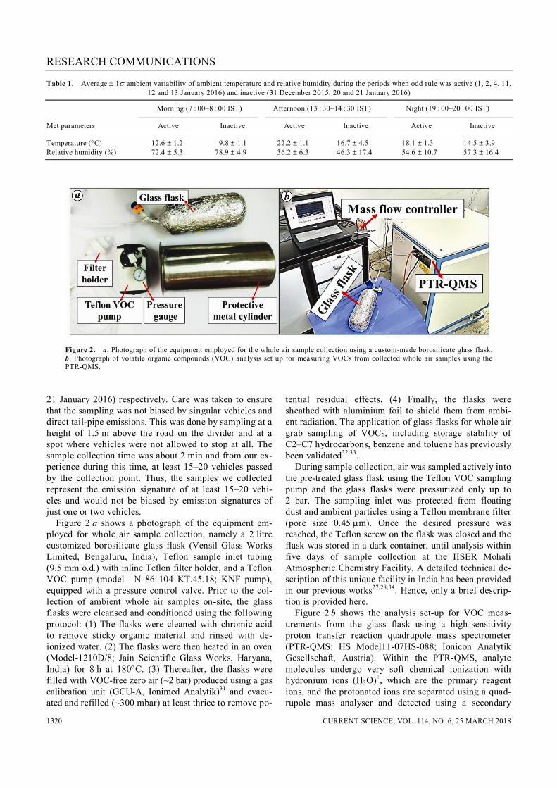
Figure 2. a, Photograph of the equipment employed for the whole air sample collection using a custom-made borosilicate glass flask. b, Photograph of volatile organic compounds (VOC) analysis set up for measuring VOCs from collected whole air samples using the PTR-QMS.

21 January 2016) respectively. Care was taken to ensure that the sampling was not biased by singular vehicles and direct tail-pipe emissions. This was done by sampling at a height of 1.5 m above the road on the divider and at a spot where vehicles were not allowed to stop at all. The sample collection time was about 2 min and from our ex-perience during this time, at least 15–20 vehicles passed by the collection point. Thus, the samples we collected represent the emission signature of at least 15–20 vehi-cles and would not be biased by emission signatures of just one or two vehicles. Figure 2 a shows a photograph of the equipment em-ployed for whole air sample collection, namely a 2 litre customized borosilicate glass flask (Vensil Glass Works Limited, Bengaluru, India), Teflon sample inlet tubing (9.5 mm o.d.) with inline Teflon filter holder, and a Teflon VOC pump (model – N 86 104 KT.45.18; KNF pump), equipped with a pressure control valve. Prior to the col-lection of ambient whole air samples on-site, the glass flasks were cleansed and conditioned using the following protocol: (1) The flasks were cleaned with chromic acid to remove sticky organic material and rinsed with de-ionized water. (2) The flasks were then heated in an oven (Model-1210D/8; Jain Scientific Glass Works, Haryana, India) for 8 h at 180C. (3) Thereafter, the flasks were filled with VOC-free zero air (~2 bar) produced using a gas calibration unit (GCU-A, Ionimed Analytik)31 and evacu-ated and refilled (~300 mbar) at least thrice to remove po-

tential residual effects. (4) Finally, the flasks were sheathed with aluminium foil to shield them from ambi-ent radiation. The application of glass flasks for whole air grab sampling of VOCs, including storage stability of C2–C7 hydrocarbons, benzene and toluene has previously been validated32,33. During sample collection, air was sampled actively into the pre-treated glass flask using the Teflon VOC sampling pump and the glass flasks were pressurized only up to 2 bar. The sampling inlet was protected from floating dust and ambient particles using a Teflon membrane filter (pore size 0.45 m). Once the desired pressure was reached, the Teflon screw on the flask was closed and the flask was stored in a dark container, until analysis within five days of sample collection at the IISER Mohali Atmospheric Chemistry Facility. A detailed technical de-scription of this unique facility in India has been provided in our previous works27,28,34. Hence, only a brief descrip-tion is provided here. Figure 2 b shows the analysis set-up for VOC meas-urements from the glass flask using a high-sensitivity proton transfer reaction quadrupole mass spectrometer (PTR-QMS; HS Model11-07HS-088; Ionicon Analytik Gesellschaft, Austria). Within the PTR-QMS, analyte molecules undergo very soft chemical ionization with hydronium ions (H3O)+, which are the primary reagent ions, and the protonated ions are separated using a quad-rupole mass analyser and detected using a secondary



electron multiplier27,28. Each VOC was measured with a dwell time of 1 s in selected ion-monitoring mode. The 13 VOCs, namely methanol, acetonitrile, acetaldehyde, ace-tone, dimethyl sulphide (DMS), isoprene, MVK, MEK, benzene, toluene, sum of xylene and ethylbenzene iso-mers, sum of trimethylbenzene and propylbenzene iso-mers, and monoterpenes were detected at their respective protonated organic ions (MH+): m/z 33, m/z 42, m/z 45, m/z 59, m/z 63, m/z 69, m/z 71, m/z 73, m/z 79, m/z 93, m/z 107, m/z 121 and m/z 137 respectively. These VOC identifications are in keeping with extensive validation experiments performed in a variety of ecosystems and have been reviewed in detail previously35,36. Due to iso-baric contributions of furan to the signal at m/z 69 and potential minor isobaric contributions to MVK and MEK, our measurements represent an upper limit for isoprene, MVK and MEK concentrations27,35. The sample flow (~100 ml/min) from the glass flask was regulated using a mass flow controller (MFC: EL-FLOW; Bronkhorst high-tech; stated uncertainty 2%). Calibration experiments were performed on 2 December 2015 and 15 January 2016 to determine sensitivities, by dynamic dilution of a custom-ordered VOC gas standard (Apel-Riemer Envi-ronmental, Inc., Colorado, USA). The sensitivity factors (normalized counts per second/parts per billion (ncps/ ppb)) and measurement uncertainties for the aforemen-tioned 13 VOCs were determined according to the proto-cols detailed in our previous works27,31,34. All mixing ratios so obtained were converted to mass concentrations using the measured ambient temperatures and pressures rele-vant for the sample. The total measurement uncertainties were as follows: methanol, acetonitrile, acetaldehyde, ace-tone, benzene and toluene (<15%), acetonitrile, DMS, isoprene, MEK and MVK (<20%), and sum of xylenes and ethylbenzene isomers, sum of trimethylbenzenes and propylbenzene isomers and monoterpenes (<25%). The limit of detection (2 noise while sampling VOC-free air) ranged between 0.03 and 0.15 g m–3, and was never an issue for any of the ambient air samples from Delhi. Carbon dioxide (CO2) and methane (CH4) were meas-ured using a cavity ring down spectrometer (CRDS; Model G2508, Picarro, Santa Clara, USA), whereas car-bon monoxide (CO) was measured using a non-dispersive infrared (NDIR) filter correlation spectrometer (Thermo Fisher Scientific, Model No. 48i), as described in our previous work27,28. Calibration experiments were per-formed for the CRDS instrument by dynamic dilution of a gas standard mixture of CO2 and CH4 (Phoenix Gases Ltd, Navi Mumbai, India; traceable to NIST, USA) on 19 December 2015, and for the CO analyser on 12 December 2015 and 19 January 2016 by dynamic dilution of a gas standard (Chemtron Science Laboratories Pvt Ltd, Mumbai) respectively. The total uncertainty for the CO measurements was always below 6% and for the meas-urements of CO2 and CH4 it was <4% in each case. The limit of detection for CO2, CH4 and CO was below 0.5,

0.2 and 12 g m–3 respectively. Concentrations of CO2 and CH4 reported in this study were corrected for the dilution and broadening effect due to the presence of water vapour37. Figure 3 presents a summary of the average VOC frac-tional contributions to the total measured VOC mass con-centration (g m–3) for the morning (7 : 00–8 : 00 IST), afternoon (13 : 30–14 : 30 IST) and night–time (19 : 00–20 : 00 IST) during both OA and OI periods. Also shown as red, blue and black histograms are the average meas-ured mass concentrations (g m–3) of CO2, CH4 and CO respectively. Vertical bars on the histograms represent the 1 measurement uncertainty. The average mass con-centration ranking of measured species was characteristic of traffic plumes38–40, the same in all the collected sam-ples (n = 27) and as follows: CO2 (OAavg = 997.8 mg m–3; OIavg = 930.7 mg m–3) > CO (OAavg = 3.9 mg m–3; OIavg = 4.2 mg m–3) > CH4 (OAavg = 2.7 mg m–3; OIavg = 2.2 mg m–3) > toluene (OAavg = 90.7 g m–3; OIavg = 71.3 g m–3) > sum of xylenes and ethylbenzene isomers (OAavg = 77.6 g m–3; OIavg = 61.6 g m–3) > sum of trimethylbenzenes and propylbenzene isomers (OAavg = 45.5 g m–3; OIavg = 36.3 g m–3) > methanol (OAavg = 56.3 g m–3; OIavg = 40.1 g m–3) > benzene (OAavg = 40.0 g m–3; OIavg = 34.3 g m–3) > acetone (OAavg = 30.4 g m–3; OIavg = 22.6 g m–3) > acetaldehyde (OAavg = 30.4 g m–3; OIavg = 22.6 g m–3) > sum of isoprene and furan (OAavg = 16.7 g m–3; OIavg = 12.0 g m–3) > methyl ethylketone (OAavg = 9.8 g m–3; OIavg = 6.2 g m–3) > methyl vinyl ketone (OAavg = 7.9 g m–3; OIavg = 5.6 g m–3) > aceto-nitrile (OAavg = 4.0 g m–3; OIavg = 3.0 g m–3) > mono-terpenes (OAavg = 2.5 g m–3; OIavg = 1.7 g m–3) > dimethyl sulphide (OAavg = 1.2 g m–3; OIavg = 1.1 g m–3). The total fraction of measured aromatic mass concentra-tions (105.0–351.6 g m–3; sum of benzene, toluene, sum of xylenes and ethylbenzene isomers and sum of trime-thylbenzenes and propylbenzene isomers) accounted for 55–70% of the total measured VOC mass concentrations in all samples. It is worth mentioning that in ambient sur-face air at sites where the chemical composition is not controlled by primary traffic emissions, the sum of oxy-genated VOCs such as methanol, acetaldehyde, acetone, MVK and MEK typically exceeds the sum of the concen-tration of aromatic compounds such as benzene, toluene, sum of xylenes and ethylbenzene isomers and sum of trimethylbenzene and propylbenzene isomers, as reported in previous studies27,41. Toluene and alkyl benzenes are major constituents of automobile exhaust16,17, in part because of the use of such compounds and their deriva-tives as additives that improve the fuel octane rating and anti-knock properties. Table 2 shows a comparison of the average concentration (g m–3) acquired in the present study for benzene, toluene and sum of xylenes and ethyl-benzene isomers and their concentration ranking (tolu-ene > sum of xylenes and ethylbenzene isomers > benzene) with traffic sites in the UK42, Algeria43 and



Figure 3 a–f. Pie charts summarizing VOC speciation during odd–even rule active days and odd–even rule inactive days derived from the meas-urements (n) at IOCL traffic thorough fare, New Delhi. Each fraction in each pie chart represents the respective averaged measured VOC mass con-centration (g m–3). Highlighted fraction of each pie chart with a black line shows the total fraction of measured aromatic mass concentration in the total measured VOC mass concentration in g m–3 1 standard deviation (total measurement uncertainty). Inserted red, blue and black histograms are the average measured mass concentration of carbon dioxide, methane and carbon monoxide respectively. Vertical bars represent the total meas-urement uncertainty as standard deviation. previous traffic emission studies in Kolkata44 and Delhi45. Direct comparison of the absolute VOC concentration values in different studies should be treated with caution as the type of fuel, traffic density and meteorological conditions can induce large variability, but toluene (T) to benzene (B) concentration ratios are better indicators for

characterizing traffic plume signatures. We note that the (T/B) concentration ratios greater than 1 are characteristic of traffic emission ratios, and considering ambient vari-ability of individual datasets (T/B = 2.7 0.2 during OA and T/B = 2.1 0.8 during OI), comparable to the T/B ratios reported from traffic plumes in Birmingham, UK



Table 2. Comparison of average benzene, toluene and sum of xylene and ethyl benzene isomer concentrations (g m–3) and aver-age ratio of toluene to benzene measured at sampling site (28.57N, 77.11E, 220 amsl) with road-side measurements at selected sites elsewhere in the world

Sum of xylene Location Benzene (B) Toluene (T) and ethylbenzene isomers Average T/B ratio

Birmingham, UKa 49.6 108.1 69.5 2.2 Algiers, Algeriab 27.1 39.2 33.1 1.5 Kolkata, Indiac 30.8 52.1 48.5 1.7 Delhi (Connaught Place), Indiad 97 180 144 1.9 Delhi (Okhla), Indiad 89 204 118 2.3 Delhi (AIIMS), Indiad 110 191 155 1.7 Delhi (IOCL traffic junction), Indiae 38.1 84.3 72.3 2.2

aKim et al.42, bKerbachi et al.43, cSom et al.44, dHoque et al.45, ePresent study. (2.2)42; Algiers, Algeria (1.5)43; Kolkata (1.7)44; Con-naught Place, Delhi (1.9)45; Okhla, Delhi (2.3)45 and AIIMS, Delhi (1.7)45. The average mass concentration in morning samples collected between 7 and 8 a.m. local time for all meas-ured VOCs during OA period was 436.6 161.5 g m–3 out of which aromatic compounds contributed 256.0 32.2 g m–3 (note numbers are: average 1 ambient variability). These are 1.6 times higher than the average of all measured VOCs during the OI period of 269.2 124.3 g m–3. This suggests that a large number of per-sonal vehicle users may have opted to commute before the traffic restrictions were put in place (odd–even rule enforcement timings were 8 a.m.–8 p.m.). In the after-noon, during the OA period, the measured average total mass concentration of VOCs was 256.0 32.2 g m–3, while that of the total aromatic compounds was 153.9 23.5 g m–3, which is about 1.4 times higher compared to corresponding OI period values. Note that this is despite the OA period being characterized by warmer afternoons and hence potentially higher mixed depth layer and dilu-tion (Tavg,OA = 22.2C versus Tavg,IA = 16.7C). Given the fact that during the OA period there was an overall in-crease reported in the number of vehicles that were ex-empt from the rule such as motorized two-wheelers (12%), three-wheelers (12%), taxis (22%) and buses (138%)13, and the fact that two-wheelers have higher emissions per unit than cars fitted with latest emission control technology4,46, the combination can explain the observed data. In the night-time, average measured mass concentrations of VOCs were comparable within the 1 ambient variability range. We further employed robust statistics (Mann–Whitney U)47 to test for statistically significant differences, if any, for the median concentrations of the measured VOCs and trace gases in samples collected during the OA and OI periods. The results are as under: (i) Median concentrations for the morning samples were significantly higher (confidence interval 84% or p 0.16) during the OA period for all compounds, except benzene, CO and acetonitrile. It is worth mentioning that

neither benzene nor CO nor acetonitrile has traffic as its dominant source. (ii) Median concentrations for the afternoon samples were also significantly higher (confidence interval >90% or p < 0.1) during the OA period for all compounds, except methane, methanol and DMS. (iii) Median concentrations for the night-time samples did not have statistically significant differences between OA and OI periods. In view of the obtained experimental data and statisti-cal test results, we conclude that the odd–even rule policy measure did not result in reduction of primary traffic emissions. Instead, it appears that there was an overall in-crease in traffic emissions, likely due to the changed tem-poral and fleet emission behaviour triggered in response to the rule. Two factors combined together can help explain the higher traffic emissions observed during the period when the odd–even rule was enforced. The first is that a large number of personal vehicle users seem to have opted to commute before the traffic restrictions were put in place. Secondly, there was an overall increase re-ported in the number of vehicles that were exempt from the rule, such as motorized two-wheelers, three-wheelers, taxis and buses by 12–138% (ref. 46). The emissions from the increased fleet of exempt vehicles therefore appear to have offset the reduction of emissions accom-plished by controlling personal four-wheeler vehicles/ cars. Another point worth considering is that the odd–even rule may have resulted in traffic decongestion dur-ing peak hours, which may certainly have benefited commuters. However, it must also be kept in mind that enhanced traffic emissions during times of the day when the dilution effect due to the atmospheric boundary layer is low (e.g. early morning before 8 a.m. and at night after sunset), could lead to higher peak concentration exposure for several health-relevant carcinogenic VOCs such as benzene. While several important insights have been gained through this study, for future assessment studies, it would be advisable to deploy on-line VOC measurements of the kind reported here at multiple strategic sites as part of the



experimental design. Further, combining measurements of tail-pipe emissions from key major vehicle types ply-ing on the roads along with information about the number and type of vehicle (e.g. through webcam recordings at sampling points), would help provide more detailed information concerning the major emitters. Such an ex-perimental design would also help address current uncer-tainties with regard to quantitative source apportionment of air pollutants in Delhi, similar to that demonstrated re-cently by some of us for the Kathmandu Valley41,48, and enable air-pollution mitigation efforts for multiple urban sources rather than just traffic emissions.

1. United Nations, World’s population increasingly urban with more than half living in urban areas, 2014; available at: http:// wwwunorg/en/development/desa/news/population/world-urbanization-prospects-2014.html

2. Nagpure, A. S., Gurjar, B. R. and Martel, J., Human health risks in national capital territory of Delhi due to air pollution. Atmos. Pol-lut. Res., 2014, 5(3), 371–380.

3. Guttikunda, S. K. and Calori, G., A GIS based emissions inven-tory at 1 km 1 km spatial resolution for air pollution analysis in Delhi, India. Atmos. Environ., 2013, 67, 101–111.

4. Sindhwani, R. and Goyal, P., Assessment of traffic-generated gaseous and particulate matter emissions and trends over Delhi (2000–2010). Atmos. Pollut. Res., 2014, 5, 438–446.

5. Delhi Statistical Handbook 2016, Directorate of Economics and Statistics, Government of National Capital Territory of Delhi, 2016; pp. 210–211; http://www.delhi.gov.in/wps/wcm/connect/ doit_des/DES/Our+Services/Statistical+Hand+Book/

6. World Health Organization, WHO’s urban ambient air pollution database. 2016; http://www.who.int/phe/health_topics/outdoorair/ databases/AAP_database_summary_results_2016_v02.pdf?ua=1

7. Goel, R. and Guttikunda, S. K., Role of urban growth, technology, and judicial interventions on vehicle exhaust emissions in Delhi for 1991–2014 and 2014–2030 periods. Environ. Dev., 2015, 14, 6–21.

8. Beig, G. et al., Quantifying the effect of air quality control meas-ures during the 2010 Commonwealth Games at Delhi, India. Atmos. Environ., 2013, 80, 455–463.

9. Davis, L. W., The effect of driving restrictions on air quality in Mexico City. J. Polit. Econ., 2008, 116, 38–81.

10. Tan, Z. et al., Evaluating vehicle emission control policies using on-road mobile measurements and continuous wavelet transform: a case study during the Asia–Pacific Economic Cooperation Forum, China, 2014. Atmos. Chem. Phys. Discuss, 2016, 2016, 1–39.

11. Mahendra, A., Vehicle restrictions in four Latin American cities: is congestion pricing possible? Trans. Rev., 2008, 28, 105–133.

12. Odd–even scheme. Government of National Capital Territory of Delhi, Transport Department, 28 December 2015; http://it. delhigovt.nic.in/writereaddata/egaz20157544.pdf

13. Goyal, P. and Gandhi, G., Assessment of air quality during the ‘odd–even scheme’ of vehicles in Delhi. Indian J. Sci. Technol., 2016, 9(48).

14. Singhania, K., Girish, G. and Vincent, E. N., Impact of odd–even rationing of vehicular movement in Delhi on air pollution levels. Low Carbon Econ., 2016, 7, 151.

15. Pavani, V. S. and Aryasri, A. R., Pollution control through odd–even rule: a case study of Delhi. Indian J. Sci., 2016, 23, 403–411.

16. Henze, D. K. et al., Global modeling of secondary organic aerosol formation from aromatic hydrocarbons: high- vs low-yield path-ways. Atmos. Chem. Phys., 2008, 8, 2405–2420.

17. Singh, H. B., Salas, L. J., Cantrell, B. K. and Redmond, R. M., Distribution of aromatic hydrocarbons in the ambient air. Atmos. Environ., 1985, 19, 1911–1919.

18. Parrish, D. D. et al., Comparison of air pollutant emissions among mega-cities. Atmos. Environ., 2009, 43, 6435–6441.

19. Baker, A. K. et al., Measurements of nonmethane hydrocarbons in 28 United States cities. Atmos. Environ., 2008, 42, 170–182.

20. Li, S., Chen, S., Zhu, L., Chen, X., Yao, C. and Shen, X., Concen-trations and risk assessment of selected monoaromatic hydrocar-bons in buses and bus stations of Hangzhou, China. Sci. Total Environ., 2009, 407, 2004–2011.

21. Holzinger, R. et al., Biomass burning as a source of formaldehyde, acetaldehyde, methanol, acetone, acetonitrile, and hydrogen cya-nide. Geophys. Res. Lett., 1999, 26, 1161–1164.

22. Mellouki, A., Wallington, T. J. and Chen, J., Atmospheric chemis-try of oxygenated volatile organic compounds: impacts on air quality and climate. Chem. Rev., 2015, 115, 3984–4014.

23. Guenther, A., Karl, T., Harley, P., Wiedinmyer, C., Palmer, P. I. and Geron, C., Estimates of global terrestrial isoprene emissions using MEGAN (Model of Emissions of Gases and Aerosols from Nature). Atmos. Chem. Phys., 2006, 6, 3181–3210.

24. Borbon, A., Fontaine, H., Veillerot, M., Locoge, N., Galloo, J. C. and Guillermo, R., An investigation into the traffic-related frac-tion of isoprene at an urban location. Atmos. Environ., 2001, 35, 3749–3760.

25. Holzinger, R., Jordan, A., Hansel, A. and Lindinger, W., Automo-bile emissions of acetonitrile: assessment of its contribution to the global source. J. Atmos. Chem., 2001, 38, 187–193.

26. Ban-Weiss, G. A., McLaughlin, J. P., Harley, R. A., Kean, A. J., Grosjean, E. and Grosjean, D., Carbonyl and nitrogen dioxide emissions from gasoline- and diesel-powered motor vehicles. Environ. Sci. Technol., 2008, 42, 3944–3950.

27. Sinha, V., Kumar, V. and Sarkar, C., Chemical composition of pre-monsoon air in the Indo-Gangetic Plain measured using a new air quality facility and PTR-MS: high surface ozone and strong in-fluence of biomass burning. Atmos. Chem. Phys., 2014, 14, 5921–5941.

28. Sarkar, C., Kumar, V. and Sinha, V., Massive emissions of car-cinogenic benzenoids from paddy residue burning in North India. Curr. Sci., 2013, 104, 1703–1706.

29. Basu, I., Squeezed into a jam in Dwarka. The Times of India, 23 February 2013, New Delhi.

30. Ghude, S. D. et al., Winter fog experiment over the Indo-Gangetic plains of India. Curr. Sci., 2017, 112, 767–784.

31. Kumar, V. and Sinha, V., VOC–OHM: a new technique for rapid measurements of ambient total OH reactivity and volatile organic compounds using a single proton transfer reaction mass spec-trometer. Int. J. Mass Spectrom., 2014, 374, 55–63.

32. Pollmann, J., Helmig, D., Hueber, J., Plass-Dülmer, C. and Tans, P., Sampling, storage, and analysis of C2–C7 non-methane hydro-carbons from the US National Oceanic and Atmospheric Admini-stration Cooperative Air Sampling Network glass flasks. J. Chromatogr. A, 2008, 1188, 75–87.

33. Chandra, B. P., Sinha, V., Hakkim, H. and Sinha, B., Storage sta-bility studies and field application of low cost glass flasks for analyses of thirteen ambient VOCS using proton transfer reaction mass spectrometry. Int. J. Mass Spectrom., 2017, 419, 11–19.

34. Chandra, B. P. and Sinha, V., Contribution of post-harvest agricul-tural paddy residue fires in the N.W. Indo-Gangetic Plain to ambi-ent carcinogenic benzenoids, toxic isocyanic acid and carbon monoxide. Environ. Int., 2016, 88, 187–197.

35. de Gouw, J. and Warneke, C., Measurements of volatile organic compounds in the earth’s atmosphere using proton-transfer-reaction mass spectrometry. Mass Spectrom. Rev., 2007, 26, 223–257.

36. Blake, R. S., Monks, P. S. and Ellis, A. M., Proton-transfer reac-tion mass spectrometry. Chem. Rev., 2009, 109, 861–896.



*For correspondence. (e-mail: [email protected])

37. Rella, C. W. et al., High accuracy measurements of dry mole frac-tions of carbon dioxide and methane in humid air. Atmos. Meas. Tech., 2013, 6, 837–860.

38. Ho, K. et al., Vehicular emission of volatile organic compounds (VOCs) from a tunnel study in Hong Kong. Atmos. Chem. Phys., 2009, 9, 7491–7504.

39. Baudic, A. et al., Seasonal variability and source apportionment of volatile organic compounds (VOCs) in the Paris megacity (France). Atmos. Chem. Phys., 2016, 16, 11961–11989.

40. Barletta, B., Meinardi, S., Simpson, I. J., Khwaja, H. A., Blake, D. R. and Rowland, F. S., Mixing ratios of volatile organic com-pounds (VOCs) in the atmosphere of Karachi, Pakistan. Atmos. Environ., 2002, 36, 3429–3443.

41. Sarkar, C. et al., Overview of VOC emissions and chemistry from PTR-TOF-MS measurements during the SusKat-ABC campaign: high acetaldehyde, isoprene and isocyanic acid in wintertime air of the Kathmandu Valley. Atmos. Chem. Phys., 2016, 16, 3979–4003.

42. Kim, Y. M., Harrad, S. and Harrison, R. M., Concentrations and sources of VOCs in urban domestic and public microenviron-ments. Environ. Sci. Technol., 2001, 35, 997–1004.

43. Kerbachi, R., Boughedaoui, M., Bounoua, L. and Keddam, M., Ambient air pollution by aromatic hydrocarbons in Algiers. Atmos. Environ., 2006, 40, 3995–4003.

44. Som, D., Dutta, C., Chatterjee, A., Mallick, D., Jana, T. K. and Sen, S., Studies on commuters’ exposure to BTEX in passen-ger cars in Kolkata, India. Sci. Total Environ., 2007, 372, 426–432.

45. Hoque, R. R., Khillare, P. S., Agarwal, T., Shridhar, V. and Bala-chandran, S., Spatial and temporal variation of BTEX in the urban atmosphere of Delhi, India. Sci. Total Environ., 2008, 392, 30–40.

46. Goyal, P., Mishra, D. and Kumar, A., Vehicular emission inven-tory of criteria pollutants in Delhi. Springer Plus., 2013, 2(216), 1–11.

47. Sheskin, D. J., Handbook of Parametric and Nonparametric Sta-tistical Procedures, Chapman & Hall/CRC, 2011, 5th edn, pp. 513–525.

48. Sarkar, C., Sinha, V., Sinha, B., Panday, A. K., Rupakheti, M. and Lawrence, M. G., Source apportionment of NMVOCs in the Kath-mandu Valley during the SusKat-ABC international field cam-paign using positive matrix factorization. Atmos. Chem. Phys., 2017, 17, 8129–8156.

ACKNOWLEDGEMENTS. We thank Prof. N. Sathyamurthy (foun-der Director, Indian Institute of Science Education and Research (IISER), Mohali), the Director General of India Meteorological De-partment, New Delhi and Professor G. S. Bhat (Indian Institute of Sci-ence, Bengaluru) for support. We also thank the IISER Mohali Atmospheric Chemistry Facility; Indian Institute of Tropical Meteoro-logy, Pune; Ministry of Human Resource Development and Ministry of Earth Sciences, Government of India for support and funding. B.P.C. thanks the Council of Scientific Industrial Research, New Delhi for SRF. Received 19 April 2017; revised accepted 5 October 2017 doi: 10.18520/cs/v114/i06/1318-1325

Effective weed control strategy in tomato kitchen gardens – herbicides, mulching or manual weeding Daud Ahmad Awan1, Faheem Ahmad2,* and Sharmin Ashraf1 1Centre for Agriculture and Biosciences International (CABI) Central and West Asia, Data Ganj Bakhsh Road, Satellite Town, Rawalpindi 46300, Pakistan 2COMSATS Institute of Information Technology, Park Road, Tarlai Kalan, Islamabad 45550, Pakistan Effect of weed control on tomato (Solanum lycopersi-cum L.) crop has been rarely explored in kitchen gar-dens for improving fruit yield and quality. Therefore, we studied the impact of manual weeding, herbicide application and mulching (using polyethylene sheet) on tomato crop improvement in kitchen gardens. The data show significant differences among different treatments in terms of weed density/m2, weed fresh biomass and dry biomass and quality of tomato plants in terms of plant height, fruit-bearing (fruits/plant) and yield (tonne/ha). Highest weed density/m2 (3.5 0.84) was observed in plots with herbicide treatment and it was similar to that in control. Weed fresh bio-mass was significantly reduced in all treatments. Manual weeding resulted in the highest number of fruits/plant (33.75 1.67), plant height (60 1.01 cm) and yield of tomato (4.45 0.18 tonne/ha). Therefore, manual control proved to be the most effective treat-ment in terms of weed suppression and yield en-hancement of tomato crop. It was also observed that in crop production mulching must be encouraged in the future weed management strategies. Keywords: Herbicide, kitchen gardens, tomato, mulch-ing, weed control. TOMATO (Solanum lycopersicum L., Solanaceae) is a popular and nutritive vegetable crop ranking next to po-tato in the world’s vegetable production1. It is an impor-tant source of minerals and antioxidants, including carotenoids, lycopene, vitamins C and E, and phenolic compounds, which play a key role in human nutrition in preventing certain cancers and cardiovascular diseases2. Being one of the most favourite vegetables, tomato is consumed in many ways3. Several factors are responsible for low yields of tomato. Among them, weed infestation in cultivated fields is the major factor which also reduces quality and value of the crop by competing for light, space and nutri-ents. Thus the farmer ends up spending more on agro-nomic practices4. On the other hand, weeds provide a safe harbour to many insect pests of tomatoes.

odd–even traffic rule implementation during winter 2016 in …€“even traffic... ·...

Documents