QUANTIFYING UNCERTAINTIES IN ESTIMATESOF INCOME AND WEALTH INEQUALITY

MARTA BOCZON

OCTOBER, 2020

(CLICK HERE FOR THE LATEST VERSION)

Abstract. I measure the uncertainty affecting estimates of economic inequality in the USand investigate how accounting for properly estimated standard errors can affect the resultsof empirical and structural macroeconomic studies. In my analysis, I rely upon two datasets: the Survey of Consumer Finances (SCF), which is a triennial survey of householdfinancial condition, and the Individual Tax Model Public Use File (PUF), an annual sampleof individual income tax returns. While focusing on the six income and wealth shares ofthe top 10 to the top 0.01 percent between 1988 and 2018, my results suggest that ignoringuncertainties in estimated wealth and income shares can lead to erroneous conclusions aboutthe current state of the economy and, therefore, lead to inaccurate predictions and ineffectivepolicy recommendations. My analysis suggests that for the six top-decile income sharesunder consideration, the PUF estimates are considerably better than those constructedusing the SCF; for wealth shares of the top 10 to the top 0.5 percent, the SCF estimatesappear to be more reliable than the PUF estimates; finally, for the two most granular wealthshares, the top 0.1 and 0.01 percent, both data sets present non-trivial challenges that cannotbe readily addressed.

1. Introduction

As of 2018, more than 40 percent of income was earned by the top 10 percent, and more

than 30 percent by the top 5 percent. In relation to wealth, more than 75 percent was owned

Key words and phrases. Survey of Consumer Finances, Statistics of Income’s Public-Use Microdata

Files, Total Survey Error. JEL: C63, C82, C83, G50, G51.

Author: Boczon: Department of Economics, University of Pittsburgh, 230 South Bouquet Street, Wesley

W. Posvar Hall, Pittsburgh PA, 15213. E-mail: martaboczon@pitt.edu. Foremost, I would like to express my

sincere gratitude to my supervisor Jean-Francois Richard, to whom I would like to dedicate this project, for

his continuous support throughout my Ph.D. studies and particularly for his dedication, encouragement, and

immense knowledge. He has been not only my primary advisor but also my mentor. Besides my supervisor, I

would like to thank the rest of my thesis committee: Arie Beresteanu, Roman Liesenfeld, and Alistair Wilson

for their motivation and insightful comments. My completion of this project could not have been possible

without the support of Jesse Bricker, John Czajka, Daniel Feenberg, Kevin Moore, William Peterman, and

Allison Schertzer. For helpful feedback, I also thank Claudia Sahm, Janine Carlock, and the University of

Pittsburgh Writing Center. Lastly, I am grateful to the Federal Reserve Board of Governors Dissertation

Internship program for research support. Remaining errors are my sole responsibility.1

arX

iv:2

010.

1126

1v1

[ec

on.G

N]

21

Oct

202

0

by the top 10 percent, and more than 65 percent by the top 5 percent. According to Saez

(2017), the last time we observed comparably high levels of top income and wealth inequality

was in the years leading to the 1929–1933 Great Depression.

Inequality endangers the economy in a number of ways: it threatens the integrity of economic

systems and the impartiality of political institutions, and eventually can lead to a rise of

extremism or even oligarchies. So far, income and wealth inequality in the US has been

linked to declining trust in political institutions, low voter turnout, political polarization,

declining life expectancy, and a rise in obesity, mental illness, homicide, teenage pregnancy,

and substance abuse. For example, Saez and Zucman (2019) find that rich Americans live

almost 15 years longer than poor ones. This represents a gap in life expectancy comparable

to that between the US and Nigeria. Moreover, rising income and wealth concentration in

the US endangers equal distribution of economic resources around the world. In particular,

between 1970 and 1992 an increase in the number of “globally rich” in the US, defined

as those with more than twenty times the mean world income, accounted for half of the

worldwide increase, making “a perceptible difference to the world distribution” (Atkinson et

al., 2011).

While numerous studies, including Piketty and Saez (2003), Atkinson et al. (2011), Bricker

et al. (2016), Bricker et al. (2018), and Saez and Zucman (2016, 2020b) estimate income and

wealth inequality, few examine the statistical uncertainty around their estimates. However,

this is of great importance, since such uncertainties could lead to erroneous conclusions

about the current state of the economy and, therefore, result in inaccurate predictions and

ineffective policy recommendations.

During the past two years, economists and politicians have discussed various measures aimed

at combating inequality: instituting a wealth tax on millionaires, raising the top income tax

rate, reducing exemptions and increasing tax rates on large estates. However, whether such

policies would prove effective at closing the gap between rich and poor depends primarily

on our ability to produce statistically accurate estimates of income and wealth inequality.

Otherwise, the government might collect either too little in tax revenue, unable to provide

the poor with adequate government-funded child care and paid-leave, or too much, causing

a sudden and sharp decline in economic growth.

Moreover, since income and wealth inequality has been at the center of attention during the

2020 Democratic Party presidential primaries, it is imperative to provide the general public

with an idea of the accuracy of these estimates. Otherwise, the public could easily be misled

to either under- or overestimate the severity of the ongoing crisis linked to rising inequality.2

This, in turn, may result in voters misconstruing the effectiveness of current policies and

lead them to express support for more conservative proposals.

In this paper, I estimate the uncertainties in estimates of the six income and wealth shares of

the top 10 to the top 0.01 percent (the American upper middle and upper classes) and assess

their impact on both empirical and structural macroeconomic studies. To do this, I first

investigate which data set proves most credible for studying income and wealth concentration.

Second, I analyze whether my results regarding the magnitudes and trends in top income

and wealth inequality support or contradict those published in the related literature. Finally,

I examine to what extent uncertainties in calibration targets affect outcomes of structural

macroeconomic modeling, in the context of a random growth model of income.

The present paper contributes to the existing literature on economic inequality in five main

ways. First, it adds to our understanding of the types of error that are most prevalent in

estimates of income and wealth inequality. Second, it provides a cost-benefit analysis of

studying economic inequality using survey data (with a wide range of both financial and

nonfinancial variables but a small number of observations) versus administrative tax records

(with a large number of observations but no information on taxpayers’ demographic or socio-

economic characteristics). Third, it introduces a novel approach to estimating sampling error

using administrative tax data, with a focus on the context of economic inequality. Fourth, it

is the first research project to estimate the long-term dynamics in economic inequality while

accounting for uncertainties in the constructed estimates of top income and wealth shares.

Finally, it discusses the consequences of utilizing error-prone data for structural analysis,

including data tracking and projecting.

In this paper, I define income as gross income comprising all income items except for capital

gains and wealth as all assets less all liabilities. For both the empirical and structural

analysis, I use two data sets: the Survey of Consumer Finances (SCF)—a triennial survey of

US household financial condition—and the Individual Tax Model Public Use File (PUF)—

an annual sample of US individual income tax returns. The SCF survey data range from

1988 to 2018, and the PUF administrative data range from 1991 to 2012 (the 2018 SCF

and the 2012 PUF are the latest available data sets at the time of writing). Consequently,

my analysis focuses on the over twenty-year long period that follows the Tax Reform Act

of 1986, which lowered federal income tax rates and, in particular, reduced the top tax rate

from 50 to 28 percent.

In order to determine which data source is more reliable for studying top income and wealth

inequality, I compare the SCF survey data and the PUF administrative data with respect

to a number of criteria, such as the total and weighted number of observations available for3

the estimation and the size of relative standard errors. For studying long-term dynamics in

income and wealth inequality, I use weighted least squares with weights defined as reciprocals

of squared standard errors. In addition to long-term trends, I examine how income and

wealth concentration changed between the onset and the aftermath of the 2007–2009 Great

Recessions.

In addition to accounting for data-driven errors in empirical analysis of top-decile income

and wealth shares, I investigate how data deficiencies affect outcomes of structural macroe-

conomic models. I consider the augmented random growth model of income proposed by

Gabaix et al. (2016) and use Monte-Carlo simulation techniques to analyze how errors in in-

puts to this model impact the precision of the model’s outcomes. Specifically, for each of the

two data sets under consideration, I calibrate Gabaix et al. (2016)’s model multiple times,

each time using a different value randomly drawn from a confidence interval constructed

around the point estimate of the model’s calibration target. Then, by averaging over the

range of generated model outcomes, I determine the extent to which the model’s outputs are

affected by the uncertainty in the model’s inputs.

My empirical analysis of top income inequality suggests that estimates constructed using

the administrative data are considerably better than those constructed using the survey

data. One of the advantages of using the PUF is its higher data frequency and the fact

that sampling error in the estimated income shares is on average five times smaller than in

the SCF. While these data features are not critical when examining long-term dynamics of

income inequality, they become a decisive factor when choosing between the SCF and the

PUF in a study that analyzes short-time horizons and year-to-year changes. Moreover, the

small number of observations above the 99.9 and 99.99 income fractiles in the SCF makes

the SCF estimates of the two most granular income shares of the top 0.1 and 0.01 percent

extremely volatile and, thus, uninformative.

In relation to wealth inequality, my empirical results indicate that neither the survey data nor

the administrative data can be used without caution. For the less granular wealth shares

of the top 10 to the top 0.5 percent, I find the SCF more reliable than the PUF. In the

SCF, respondents are asked about their asset and liability holdings, whereas in the PUF,

the wealth of every individual in the sample is estimated from their reported income using

a capitalization model. Since such models are heavily dependent on numerous (and often

arbitrary) assumptions imposed on assets’ rates of return, so are the resulting estimates of

top wealth shares. Therefore, even though the SCF estimates have larger sampling errors

than those constructed using the PUF, they are free from non-trivial and yet-to-be-fully-

determined modeling errors arising in the process of inferring wealth from income. Lastly,4

regarding wealth shares of the top 0.1 and 0.01 percent, I find that both the SCF and the

PUF present difficult-to-overcome challenges (an insufficient number of observations and

modeling errors, respectively) that result in highly unreliable estimates of the far right tail

of wealth distribution of the top 0.1 and 0.01 percent.

In addition to identifying strengths and weaknesses of survey and administrative data in

studying income and wealth concentration, this paper adds new insight to the ongoing debate

regarding the magnitudes and trends in top income and wealth inequality. For income, my

results confirm those from the related literature, indicating a statistically significant increase

in income concentration between the early 1990s and the early 2010s, and suggest comparable

levels and trends in the estimated income shares within the top 10 percent.

For wealth, since this paper finds the SCF a more reliable data source than the PUF, it

portrays a different picture of top wealth inequality than the most widely-cited studies on

wealth concentration estimated using administrative tax-level data (e.g., Saez and Zucman,

2016). Specifically, while my study does suggest a statistically significant increase in the

wealth shares of the top 10, 5, and 1 percent between the early 1990s and the early 2010s,

the estimated trend lines are more modest than in Saez and Zucman (2016). Second, I do

not find evidence of rising wealth inequality within the top ten percent. Unlike Saez and

Zucman (2016) who observe a larger increase in the wealth shares of the top 1 percent than

in the wealth shares of the top 10 percent, the weighted linear regression analysis of the SCF

point estimates suggests the opposite, casting doubts on a presumption that an observed rise

in wealth inequality is driven solely by the far right tail of wealth distribution. Furthermore,

this paper does not support the authors’ widely-cited conclusion regarding a 100 percent

increase in the wealth shares of the top 0.1 percent between 1991 and 2012, a finding that

has drawn substantial media coverage and major interest from politicians and policy makers.

My third set of results pertains to the consequences of modeling inequality using error-prone

data. In relation to the Gabaix et al. (2016)’s random growth model of income, I find that

having precise estimates of calibration targets is critical for producing precise outcomes of

structural analysis. This is the case since errors in calibration targets are carried over through

the model and come to affect all outcomes of interest. Specifically, I find that the model

calibrated to administrative tax data projects income shares of the top 1 percent in 2050 to

be equal to 22.5 percent, with only negligible levels of uncertainty attributable to the data.

On the other hand, the model calibrated to survey data is much less precise regarding the

2050 projection, with a 95 confidence interval ranging from 19 to 29 percent. Therefore, by

relying upon administrative tax data for the model’s calibration, as opposed to survey data,

one can reduce the uncertainty in the model’s outcome of interest by a factor of ten.5

My paper is organized as follows. In Section 2, I discuss related literature. In Section 3, I

provide a brief description of sources of error in survey and administrative data. In Section 4,

I characterize the main features of the SCF and describe the estimation procedure of the SCF

standard error. In Section 5, which follows the same format as Section 4, I first provide a brief

description of the PUF and next, characterize the estimation of the PUF standard error. In

Section 6, I define the concepts of income and wealth and discuss the estimation procedure of

top-decile income and wealth shares. In Sections 7 and 8, I analyze the main empirical results

centered around income and wealth inequality, respectively. In Section 9, I discuss the key

outcomes of the structural analysis. Section 10 concludes. Online supplementary material

with additional results and detailed discussions supporting my conclusions is available on

https://martaboczon.com.

2. Literature review

This paper contributes to four main strands of economic literature: economic inequality,

survey statistics, SCF survey design, and PUF sample design.

First, since one of my objectives is to quantify uncertainties in estimates of income and

wealth inequality within the top 10 percent, this paper contributes to the growing body of

literature on income and wealth inequality in the US. Specifically, it is closely-related to

the work of Piketty and Saez (2003), where the authors rely upon tax returns statistics and

micro-level data on individual-income tax returns in order to construct homogeneous series of

top-decile income shares between 1913 and 1998. Another important reference the research

is related to is Atkinson et al. (2011), which utilizes individual-income tax return statistics

for numerous income brackets in order to provide a comprehensive overview and comparative

analysis of historical and current trends in top income shares for multiple countries around

the globe.

In addition, the current paper adds valuable insights to the literature on wealth inequality.

In particular, it builds on Saez and Zucman (2016) and Bricker et al. (2018), in which the au-

thors rely upon micro-level data and aggregate statistics published in the Financial Accounts

of the United States in order to estimate the distribution of wealth using a capitalization

model. Moreover, it is indirectly related to Kopczuk and Saez (2004), who estimate wealth

concentration using estate tax return data, in which individual estates are weighted by the

inverse probability of death.

Since this paper analyzes various data-driven errors in surveys and other sample data, it

constitutes a direct application of an important statistical concept related to the Total Survey

Error (TSE) paradigm. Even though, TSE has been thoroughly discussed in the literature on6

survey statistics (see, e.g. Biemer and Lyberg, 2003; Groves et al., 2009), it remains largely

ignored in economics. Therefore, this paper constitutes an example of how established and

widely applied statistical concepts can benefit economic research.

In addition to adding to economic inequality and survey statistics literature, the present

paper contributes to the literature on the SCF survey design (see, e.g. Kennickell, 1997,

1998, 2000, 2008). Specifically, except for research conducted by the Board of Governors of

the Federal Reserve System, it is the first academic paper to consider data-driven errors in

any macroeconomic estimates constructed using the SCF survey data.

Lastly, this paper contributes to the literature on the PUF sampling design (see Czajka

et al., 2014; Bryant et al., 2014). Specifically, it proposes a bootstrapping technique that

allows data users to estimate the PUF sampling error for any quantity of interest. As such, it

provides an illustrative example of how the information regarding a complex sample selection

process can be incorporated into an economic analysis.

3. Total Survey Error

Since one of my primary objectives is to identify and quantify sources of data-driven errors

in the estimates of income and wealth inequality, this paper is centered around the TSE

paradigm—an umbrella term for a variety of error sources in survey data. Even though TSE

pertains primarily to errors in surveys, it is also applicable to data consisting of administra-

tive records. This is the case since administrative data are affected by the same sources of

error as survey data. Specifically, as with any other sample, administrative data are subject

to sampling error caused by drawing a sample rather than conducting a complete census.

Moreover, the data are prone to nonsampling errors, which comprise all other sources of error

arising in the process of designing, collecting, processing, and analyzing of sample data.

TSE consists of two main components: sampling error and nonsampling error, which can be

further divided into specification, frame, nonresponse, measurement, and processing errors,

all of which I briefly characterize in the remainder of the present section.1 One of the

advantages of decomposing TSE is that it allows me to differentiate between sources of error,

and consequently, address them individually. Specifically, in the present paper, I estimate

sampling and nonresponse errors in the SCF and sampling error in the PUF. As such, I do

not account for all parts of TSE (which is beyond the scope of the present paper). Instead, I

provide qualitative evidence on which components of TSE can be considered marginal for this

particular analysis and which are likely to be non-negligible and therefore, to be accounted

for in a follow-up research project.

1In this paper, without loss of generality I rely upon a TSE decomposition from Biemer and Lyberg(2003). Alternative decomposition can be found, for example, in Groves et al. (2009).

7

Specification error occurs “when the concept implied by the survey question and the concept

that should be measured in the survey differ” (Biemer and Lyberg, 2003). This often results

from misunderstandings between the different parties involved in the survey process such as

researchers, data analysts, survey sponsors, questionnaire designers, and others.

The other sources of nonsampling error are frame and processing errors. The former relates

to the process of constructing, maintaining, and using the sampling frame for selecting

the sample, whereas the latter occurs in data editing, coding, entry of survey responses,

assignment of survey weights, tabulation and other data arrangements.2

Nonresponse encompasses unit nonresponse, item nonresponse, and incomplete response,

and is considered “a fairly general source of error” (Biemer and Lyberg, 2003). A unit

nonresponse occurs when a sampling unit does not participate in the survey; an item nonre-

ponse when a participating unit leaves a blank answer to a specific survey question; and an

incomplete response when the answer provided to a typically open-ended question is either

incomplete or inadequate.

The fifth and final source of nonsampling error, measurement error, is considered “the most

damaging source of error” (Biemer and Lyberg, 2003). It includes errors arising from respon-

dents and interviewers, in addition to other factors such as the design of the questionnaire,

mode of data collection, information system, and interview setting.

In summary, any estimator constructed using survey or sample data is subject to a variety

of sampling and nonsampling errors. Therefore, an important question is that of the extent

to which these errors can be reliably accounted for when estimating unknown population

parameters (such as top income and wealth shares) using self-reported survey data and

administrative records.

4. Uncertainties in survey data on consumer finances

The SCF is a triennial survey of household finances sponsored by the Board in cooperation

with the Statistics of Income (SOI) Division of the Internal Revenue Service (IRS).3 The

objective of the survey is to characterize the financial situations of a set of households referred

2A classic frame error occurred in a public opinion poll designed to predict the result of the 1936presidential election between Alfred Landon and Franklin D. Roosevelt. Since the sample frame was heavilyover-represented by individuals who identified as Democrats (phone owners, magazine subscribers, membersof professional associations), the difference between the poll’s prediction and the election’s result was equalto 19 percentage points and as such, constitutes the largest error ever recorded in a major public opinionpoll.

3Until 1988 the survey data were collected by the Survey Research Center at the University of Michigan.Since 1991 the data collection process has been administered by the National Opinion Research Center atthe University of Chicago.

8

to as the Primary Economic Units (PEUs), where “the PEU consists of an economically

dominant single individual or couple (married or living as partners) in a household and all

other individuals in the household who are financially interdependent with that individual

or couple.”4

The SCF was initiated in 1982 and over the years has become one of the primary data

sources in studying consumer finances. It provides exhaustive categorization and detailed

information of a variety of household financial products.5 While the most comprehensive data

are collected on household portfolios, the survey also provides supplementary information

on a wide range of demographic and socio-economic characteristics such as sex, age, race,

ethnicity, family size, homeownership status, and employment history.

Since the survey oversamples the upper tail of wealth distribution, it is also one of the

primary data sources used in studying economic inequality. However, as emphasized by the

Board, “even under ideal operational conditions, the measurements of the survey are limited

in a fundamental way by the fact that it is based on a sample of respondents rather than

the entire population.”6

In this paper, I use the SCF data between 1988 and 2018, where the 2018 SCF is the latest

available data set at the time of writing. The data sets from 1982 and 1985 are not included

as they do not provide enough information to reliably estimate the main sources of variation

in the SCF point estimates.

4.1. Estimation of the TSE. With respect to Section 3, SCF data users with access to

publicly available data files and supplementary materials can estimate two types of error,

sampling and nonresponse. Quantifying other types of error such as specification, processing,

frame, and measurement would constitute a nontrivial task that, in most instances, would

require access to undisclosed information regarding specifics of the data editing process or

construction of the sample frame, and as such is beyond the scope of the present paper.

4.1.1. Sampling error. In order to protect respondents’ confidentiality, specifics regarding

the SCF sampling design are not disclosed to the general public. This disclosure avoidance

procedure has the objective of minimizing the risk of a third party revealing the identity of a

4See the SCF codebook at https://www.federalreserve.gov/econres/files/codebk2016.txt (accessed onApril 15, 2019).

5The SCF collects information on checking, brokerage, savings, and money market accounts; certificatesof deposit; savings bonds and other types of bonds; mutual funds; publicly-traded stocks; annuities, trusts,and managed investment accounts; IRAs and Keogh accounts; life insurance policies; and other types of fi-nancial and non-financial assets; credit card debt; vehicle loans and other types of consumer loans; mortgages,lines of credit, and other loans.

6See the SCF codebook at https://www.federalreserve.gov/econres/files/codebk2016.txt (accessed onApril 15, 2019).

9

survey respondent based on the sampling-specific information such as selection probability,

sampling strata, and primary and secondary sampling units.

An important implication of this disclosure avoidance procedure is that sampling error cannot

be estimated using standard statistical techniques or built-in functions in software such as

STATA, SAS, SUDAN, or AM Statistical Software. Instead, I estimate the SCF sampling

error using bootstrapped sample replicates, generated by the Board for all survey years

between 1988 and 2018. The replicates are constructed based on the actual SCF sampling

design (see Section A.1 in Appendix A of the Online Supplementary Material) and are

provided to the general public in the form of materials supplementary to the main data set.

The main reason for providing these replicates is to facilitate the estimation of sampling error

by all SCF data users, who lack access to the undisclosed and highly confidential information

regarding the specifics of the SCF sampling design.

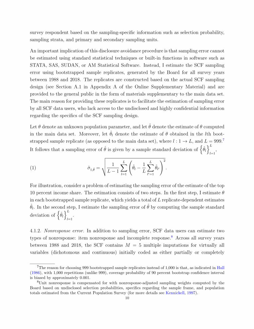
Let θ denote an unknown population parameter, and let θ denote the estimate of θ computed

in the main data set. Moreover, let θl denote the estimate of θ obtained in the lth boot-

strapped sample replicate (as opposed to the main data set), where l : 1→ L, and L = 999.7

It follows that a sampling error of θ is given by a sample standard deviation of{θl

}Ll=1

,

σ1,θ =

√√√√ 1

L− 1

L∑l=1

(θl −

1

L

L∑l′=1

θl′

)2

.(1)

For illustration, consider a problem of estimating the sampling error of the estimate of the top

10 percent income share. The estimation consists of two steps. In the first step, I estimate θ

in each bootstrapped sample replicate, which yields a total of L replicate-dependent estimates

θl. In the second step, I estimate the sampling error of θ by computing the sample standard

deviation of{θl

}Ll=1

.

4.1.2. Nonresponse error. In addition to sampling error, SCF data users can estimate two

types of nonresponse: item nonresponse and incomplete response.8 Across all survey years

between 1988 and 2018, the SCF contains M = 5 multiple imputations for virtually all

variables (dichotomous and continuous) initially coded as either partially or completely

7The reason for choosing 999 bootstrapped sample replicates instead of 1,000 is that, as indicated in Hall(1986), with 1,000 repetitions (unlike 999), coverage probability of 90 percent bootstrap confidence intervalis biased by approximately 0.001.

8Unit nonresponse is compensated for with nonresponse-adjusted sampling weights computed by theBoard based on undisclosed selection probabilities, specifics regarding the sample frame, and populationtotals estimated from the Current Population Survey (for more details see Kennickell, 1997).

10

missing.9,10,11 This data feature allows users to account for the uncertainty associated with

completely and partially missing data by estimating the variability between the multiply

imputed data sets as

σ2,θ =

√√√√ 1

M − 1

M∑m=1

(θm − θ

)2,(2)

where θm, m : 1→M denotes the estimate of θ in the mth imputation.

4.1.3. Standard error. After estimating sampling and imputation errors, I estimate the stan-

dard error of θ using Rubin’s estimator, given by:

σθ =√σ21,θ

+ σ22,θ

(1 +M−1).(3)

More details regarding Rubin’s variance estimator can be found in Section A.3 in Appendix

A of the Online Supplementary Material.

Since the above estimator of the standard error of θ (see equation 3) accounts for only two

types of error, sampling and nonresponse, it can be thought of as a lower bound on the

unknown standard error of θ, say σθ. Importantly, the degree to which σθ underestimates σθdepends on the magnitudes of the four nonsampling errors that my estimation procedure does

not account for. Given the high level of expertise of the Board in designing and supervising

the survey, I assume three of these errors—specification, processing, and frame—to be fairly

marginal. The only other type of error that may cause σθ to severely underestimate σθ is

measurement error, and more specifically, respondent-related measurement error, which I

thoroughly discuss in Section A.4 in Appendix A of the Online Supplementary Material.

5. Uncertainties in administrative data on tax returns

Starting from the early 1960s, the SOI Division of the IRS began to draw an annual sample of

the Individual and Sole Proprietorship (INSOLE) tax returns. The INSOLE sample contains

detailed information on taxpayers’ incomes, deductions, exemptions, taxes, and credits, and

thereby constitutes a micro-level database for tax policy purposes. In its present form, the

INSOLE sample contains highly sensitive information that, if made publicly available, could

risk the exposure of taxpayers’ identities. Therefore, in order to ensure full confidentiality of

9Note that since the M imputations are stored as five successive records for each survey respondent, thenumber of observations in each data set is mechanically inflated by a factor of five.

10For a general discussion on multiple imputation for nonresponse in surveys see Rubin (1987). For moreinformation on multiple imputation in the SCF see Kennickell (1998).

11See Section A.2 in Appendix A of the Online Supplementary Material for more details on partiallymissing values in the SCF.

11

the entire sample, access to the INSOLE is highly restricted and only granted to a handful

of agencies, such as the Treasury Department or Congress.

Since access to the INSOLE is strictly limited, the SOI Division annually creates another

sample of tax returns commonly referred to as the PUF. The PUF is annually sub-sampled

from the INSOLE and subjected to a number of disclosure avoidance procedures such as blur-

ring, rounding, deleting, and modifying. These techniques have the objective of ensuring that

no taxpayer can be identified from the PUF upon its release to the general public.12 Hence,

the PUF is accessible to much broader audiences, including academic and non-academic

researchers, and constitutes one of the main data sets used in studies of inequality.

In the present paper, I rely upon the PUF data between 1991 and 2012, where the 2012 PUF

is the latest available data set at the time of writing.13 As such, I analyze a twenty-two-year

period that follows the last formal redesign of the INSOLE from the late 1980s and includes

four years of the PUF after its latest revision, which took place in 2009.14

5.1. Estimation of the TSE. Contrary to popular belief, the problem of data deficiencies

pertains not only to self-reported survey data (such as the SCF) but also to data that

comprise administrative records (such as the PUF). In fact, administrative data (which until

very recently had been considered free of any source of error) are subject to the same types

of error as survey data (whose accuracy is known to be negatively affected by sampling

and nonsampling errors). Therefore, as Groen (2012) indicates, “analyses of the quality of

administrative data and reasons for differences between administrative data and survey data

are greatly needed.”15

In the present paper, I focus on the estimation of the PUF sampling error. As such, my

analysis does not account for processing, nonresponse, measurement, specification, and frame

errors. Whereas there is reason to assume that the first four types of error are marginal (see

Section B.4 in Appendix B of the Online Supplementary Material for qualitative evidence

supporting this claim), frame error may not be inconsequential.

In order to illustrate why the PUF frame error may matter, consider work by Piketty and

Saez (2003), where the authors impute income of non-filers as a fixed fraction of filers’

average income for all years between 1946 and 1998. Even though this particular imputation

12See Sections B.1 and B.2 in Appendix B of the Online Supplementary Material for a detailed descriptionof the PUF and INSOLE sampling design.

13Due to COVID-19, the release of the 2013 PUF is not known at the moment.14“The revised design modifies which returns in the INSOLE sample are excluded from the PUF, changes

the way the INSOLE sample is subsampled for the PUF, and aggregates all returns with a ‘large’ value forany specified amount variable into a single record” (Bryant et al., 2014).

15See Section 3 for a general discussion on sampling and nonsampling errors and Section B.3 in AppendixA of the Online Supplementary Material for a detailed description of different sources of error in the PUF.

12

procedure has the objective of matching the ratio (of 75–80 percent) of gross income reported

on tax returns and total personal income estimated in national accounts, it remains highly

arbitrary. As such, this and other imputation and/or estimation procedures aimed at “filling

the frame” with information on non-filers introduce additional and non-negligible sources of

error into the analysis.

5.1.1. Sampling error. Since the IRS does not provide data users with bootstrapped sample

replicates, in order to estimate the PUF sampling error I first generate L = 999 boot-

strapped sample replicates based on the publicly available information on taxpayers’ strata

and stratum-specific probability of selection. For brevity, let S denote the PUF sample of

taxpayers, and assume that S comprises J mutually exclusive and collectively exhaustive

strata such that

S = ∪Jj=1Sj,(4)

where Sj ∩ Sj′ = ∅ for all j 6= j′.

Moreover, let n denote the total sample size, and let nj be the number of taxpayers selected

for the sample from stratum j. Since the strata are mutually exclusive and collectively

exhaustive, it follows from equation (4) that

n =J∑j=1

nj.(5)

Since across all tax years under consideration there exist strata with as low as 10 observations

or fewer (see Table C.1 in Appendix C of the Online Supplementary Material), bootstrapping

methods cannot be applied directly to {Sj}Jj=1. Instead, I first classify the J strata into

J? � J clusters using the Partitioning Around Medoids (PAM) clustering procedure (see

Reynolds et al., 1992), where I determine the number of clusters in each tax year based on a

silhouette analysis. The clustering procedure uses as an input three stratification variables

originally designated for the INSOLE sample: gross income, presence or absence of special

forms and schedules, and the return’s potential usefulness for tax policy modeling. Since the

income variable is ordinal (successive income brackets) whereas the latter two are nominal,

I use the Gower distance measure, which is applicable to a mix of ordinal and nominal

variables.

The clustering procedure results in a PUF sample of taxpayers S that comprises J∗ mutually

exclusive and collectively exhaustive clusters such that

S = ∪J?

j=1S?j ,(6)

13

where S?j ∩ S?j′ = ∅ for all j 6= j′.

Moreover, with n?j denoting the number of taxpayers in cluster j, it follows from equation

(6) that

n =J?∑j=1

n?j .(7)

For example, in tax year 2008, I classify the 95 strata (with the minimum number of obser-

vations per stratum equal to 11) into 23 clusters (with the minimum number of observations

per stratum equal to 184). Summary statistics for clustered strata in the remaining tax years

(1991 through 2012) can be found in Table C.1 in Appendix C of the Online Supplementary

Material.

After classifying taxpayers into J? clusters, I draw L = 999 independent bootstrapped

sample replicates. Specifically, for each sample replicate l : 1→ L, I draw with replacement

n?j sample observations from each cluster j, such that the total number of observations in

each sample replicate is equal to n.

Finally, in order to estimate the PUF sampling error, I follow the estimation procedure of

the SCF sampling error outlined in Section 4.1.1. Let θ denote the estimate of θ computed

in the main data set, and let θl denote the estimate of θ obtained in the lth bootstrapped

sample replicate (as opposed to the main data set). I estimate the sampling error of θ by a

sample standard deviation of{θl

}Ll=1

as

σ1,θ =

√√√√ 1

L− 1

L∑l=1

(θl −

1

L

L∑l′=1

θl′

)2

.(8)

6. Income inequality measured in survey and administrative data

In the following, I first define the concept of income and wealth used throughout the paper

and next, describe the procedure for estimating top income and wealth shares in the SCF

and the PUF. Note that for the PUF, the derivations that follow apply to every tax year

between 1991 and 2012, and for the SCF, to all survey years between 1988 to 2018. The

time subscript t is omitted for ease of notation.

6.1. Income. In this paper, I define income as gross income comprising all income items,

except for capital gains, prior to deductions. The reason for excluding capital gains is that

“realized capital gains are not an annual flow of income (in general, capital gains are realized

by individuals in a lumpy way only once in a while) and form a very volatile component of14

income with large aggregate variations from year to year depending on stock price variations”

(Piketty and Saez, 2003).

The aforementioned income measure (as well as numerous alternative measures that could

be applied without loss of generality, such as gross income including capital gains) can

be constructed using each of the two data sets under consideration, without the need to

rely upon supplementary data and/or econometric modeling. Specifically, the SCF collects

information on households’ income during the SCF interview process (In total, what was your

annual income from dividends, before deductions for taxes and anything else? ), whereas the

PUF compiles income data from a sample of filed tax returns (Form 1040).16,17 The resulting

operational definitions of income are virtually identical for the two data sets, differing only

with respect to two income components: the SCF reports both taxable and nontaxable IRA

distributions and all other sources of income, the PUF reports only taxable amounts from

line 15a on Form 1040 and does not provide information on all other sources of income from

line 21.18

6.2. Wealth. Throughout my analysis, I define wealth as total assets less total debt. Since

the SCF survey participants are asked detailed questions about their asset and liability hold-

ings, measuring wealth in the SCF is straightforward and boils down to a simple accounting

exercise.19 In contrast, the PUF—a sample of individual income tax returns—provides lim-

ited information on taxpayers’ wealth, which results from the fact that many asset and

liability holdings are not reported on a tax form. For example, since for many taxpayers

standard deductions are more effective at reducing financial burden than are itemized deduc-

tions, only a small fraction of homeowners deduct mortgage interests on their tax returns.

In order to construct comprehensive wealth measures using the PUF (as well as the INSOLE

or any other tax-level data) it is necessary to rely upon auxiliary data sources and numerous

16For the SCF, I compute gross income less capital gains as a sum of salaries and wages before de-ductions for taxes (variable X5702); income from a sole proprietorship or a farm (X5704); income fromother businesses or investments; net rent, trusts, or royalties (X5714); income from non-taxable investments(X5706); income from other interest (X5708); income from dividends (X5710); income from Social Securityor other pensions; annuities, or other disability or retirement programs (X5722); income from unemploymentor worker’s compensation (X5716); income from child support or alimony (X5718); and income from othersources (X5724).

17For the PUF, I compute gross income less capital gains as a sum of wages and salaries (line 7 on Form1040); taxable interest (line 8a); tax-exempt interest (line 8b); ordinary dividends (line 9a); taxable refunds,credits, and offsets of state and local income taxes (line 10); alimony received (line 11); business and farmincome (lines 12 and 18); IRA distributions, pensions and annuities, unemployment compensation, and socialsecurity benefits (lines 15b, 16a, 19, and 20a); and rental real estate, royalties, partnerships, S corporations,and trusts (line 17).

18Note that for comparability with the PUF, I do not include welfare assistance in SCF measure of wealth.19See Figure C.1 in Appendix C of the Online Supplementary Material for a detailed description of the

construction of the SCF wealth measure.15

modeling assumptions. In this paper, I utilize a capitalization model from Saez and Zucman

(2016) and later re-visit in Bricker et al. (2018), where taxpayers’ wealth is estimated by

“capitalizing” asset income with an asset-specific rate of return. Specifically, as summarized

in Saez and Zucman (2016), for each asset class I estimate a capitalization factor that maps

the total flow of tax income to the amount of wealth from the household balance sheet of

the Financial Accounts of the United States. Then, I estimate wealth of each tax payer by

multiplying their reported incomes by the corresponding capitalization factors.

Let the wealth of taxpayer i be defined as

wealthi = nonfini +A∑a=1

incomei,ara

,(9)

where incomei,a denotes the income of taxpayer i generated by asset a = 1, · · · , A, ra de-

notes the estimated rate of return on asset a, and nonfini is the estimate of taxpayer i′s

nonfinancial wealth.

The rate of return on asset a is estimated by computing a ratio of the household stock of asset

a reported in the Financial Accounts, say FAa, to the a′s realized capital income measured

in the PUF,

ra =

∑ni=1 incomei,aFAa

.(10)

Following Saez and Zucman (2016), I organize assets from the Financial Accounts into seven

categories: (1) taxable interest-bearing assets, (2) non-taxable interest-bearing assets, (3)

dividend-generating assets, (4) assets generating profits of S corporations, (5) assets gen-

erating royalty income and profits of partnerships and C corporations, (6) tenant-occupied

real estate assets less mortgages, and (7) privately held and employer-sponsored pension

assets.20,21

For illustration, consider the following problem of determining assets of taxpayer i? with

reported income from dividends of $6,710. First, I estimate rate of return on dividend-

generating assets, say rdiv, using equation (10), with the denominator FAdiv computed

as a sum of directly held equities (FL153064105), equities indirectly held through mutual

funds (FL653064155), and the share of equities in money market funds (estimated based

on FL153034005, FL634090005, and FL633062000), less equities held by nonprofit orga-

nizations and mutual funds held in IRAs. Then, I estimate dividend-generating assets of

20In order to construct seven aggregate asset categories, it is often necessary to combine numerous linesfrom multiple tables reported in the Financial Accounts.

21Details regarding the construction of the remaining asset classes can be found on my personal websiteas well as in the Online Appendix to Saez and Zucman (2016).

16

taxpayer i? by dividing her/his dividend income of $6,710 by the estimated rate of return.

In 2012, the estimated rate of return was equal to 0.03411, implying a total of $196,717 in

dividend-generating assets for taxpayer i?.22

In this paper, I consider three sets of PUF estimates, one generated under a homogeneity

assumption imposed on all rates of return under consideration, as in equation (10), and two

sets of estimates constructed under a heterogeneity assumption, where I assume homoge-

neous rates of return on all income-generating assets except for those that generate taxable

interests. As emphasized by Bricker et al. (2018) “implied rate of return on taxable interest-

bearing assets in Saez and Zucman (2016) is much lower than market rates from the 10-year

Treasury yield or Moody’s Aaa corporate bond—the type of taxable interest-bearing assets

that are held by wealthy families (Bricker et al., 2016; Kopczuk, 2015).” Therefore, following

Bricker et al. (2018), I consider a scenario, where I assign a higher rate of return, say ra,A,

to the top 1 percent of the wealth distribution, and a lower rate, say ra,B, to the bottom 99

percent, such that

FAa =

∑i∈A incomei,a

ra,A+

∑i∈B incomei,a

ra,B,(11)

where A denotes a set comprised of the top 1 percent of the wealth distribution and B a set

comprised of the bottom 99 percent.

Note that the resulting operational definitions of wealth in the SCF and the PUF differ

with respect to three asset categories: defined pension plans and term life insurance policies,

which are included in the PUF but not in the SCF, and durable goods (e.g., vehicles), which

are included in the SCF but not in the PUF.23

6.3. Estimation. In this section, I describe the estimation procedure for top income and

wealth shares using the two data sets under consideration, the SCF survey data and the

PUF sample of administrative tax records.

22Since the Financial Accounts are revised on a quarterly basis, I use tables from the first quarter of 2020,which contain the latest data available at the time of writing.

23Sabelhaus and Henriques Volz (2019) estimate defined benefit plans for the SCF survey participantsusing an actuarial present-value model. The model utilizes information on benefit amounts for those SCFrespondents’ currently collecting a pension, the expected timing and amount of future pension benefits froma past job for those who are entitled to a benefit but are not yet collecting it, and the current wage, age,sector (private or public), and the number of years in the plan of those who have a plan tied to their currentjob but are not yet receiving benefits.

17

Let gi denote either income or wealth of observation i : 1 → n (in either the SCF or the

PUF), and let wi denote sampling weight of i such that

n∑i=1

wi = N,(12)

where N denotes the number of units in the underlying population of interest. For the SCF,

N is equal to the total number of PEUs. For the PUF, N is equal to the total number of

taxpayers.

Let g(j) be the jth-order statistic of gi, with wj denoting the sampling weight associated

with g(j).24 Moreover, let mk denote the number of observations in the bottom 100k percent

defined as

mk = kN,(13)

where k ∈ K and K = {0.9, 0.95, 0.99, 0.995, 0.999, 0.9999}.

For example, consider tax year 2008, with the number of taxpayers equal to N = 142,580,866.

It follows from equation (13) that m0.9 = 12, 322, 809 and m0.9999 = 141, 155, 090.

Next, let rk denote the unknown (income or wealth) share of the bottom 100k percent, and

let pk be the unknown share of the top 100 (1− k) percent defined as

pk = 1− rk.(14)

The estimation procedure consists of two main steps. In the first step, I determine an index

value j?k ∈ {1, · · · , n− 1} such that

j?k∑j=1

wj ≤ mk ≤j?k+1∑j=1

wj,(15)

which allows me to estimate the lower bound on rk as

rk =

∑j?kj=1wjg(j)∑nj=1wjg(j)

,(16)

and the upper bound on rk as

rk =

∑j?k+1j=1 wjg(j)∑nj=1wjg(j)

.(17)

24Order statistics of gi are ranked in ascending order of magnitude (see, e.g., David and Nagaraja, 2003)with g(1) = minj {gi} and g(n) = maxj {gi}.

18

In the second step, I estimate rk using linear interpolation between rk and rk:

rk = rk + ωk (rk − rk) ,(18)

where

ωk =mk −

∑j?kj=1wj

wj?k+1

.(19)

It follows from equation (14) that the estimator of pk is given by

pk = 1− rk.(20)

In relation to Section 4.1.2, it is important to note that since the SCF data are multiply

imputed for missing values, the aforementioned estimation procedure needs to be repeated

separately for each of the M imputed SCF data sets. This results in M estimates of pk,

which I denote as pk,m, m : 1→M . The grand estimate of pk is then obtained by averaging

over {pk,m}Mm=1 such that:

pk =1

M

M∑m=1

pk,m.(21)

7. Empirical results on income shares

In the following, I discuss my empirical results regarding the estimation of the income shares

within the top 10 percent. In Section 7.1, I compare the number of observations above top

income fractiles estimated using the the SCF and the PUF. In Sections 7.2–7.7, I focus on

point estimates, standard errors, and the long- and short-term dynamics in income inequality.

In Section 7.8, I establish a statistical link between the SCF and the PUF point estimates

for top income shares. Finally, in Section 7.9, I summarize my key findings and conclude.

7.1. Number of observations. My first set of results pertains to the number of observa-

tions in the SCF and the PUF. Across all of the years under study, I find large differences

in the number of observations between the SCF and the PUF. For example, as indicated

in Table 1, the number of observations in the SCF in 2012 accounts for just 3.5 percent

of the total number of observations available in the PUF. Moreover, since the number of

observations increases proportionately across the two data sets, the ratio of the number of

the SCF sample observations to the number of the PUF sample observations is fairly stable

across years with a minimum of 3 and a maximum of 4.5 percent.25

25See Table C.2 in Appendix C of the Online Supplementary Material for the number of observations inthe SCF and the PUF.

19

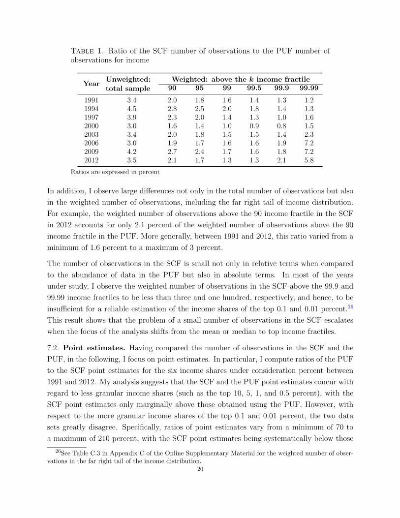
Table 1. Ratio of the SCF number of observations to the PUF number ofobservations for income

YearUnweighted:total sample

Weighted: above the k income fractile90 95 99 99.5 99.9 99.99

1991 3.4 2.0 1.8 1.6 1.4 1.3 1.21994 4.5 2.8 2.5 2.0 1.8 1.4 1.31997 3.9 2.3 2.0 1.4 1.3 1.0 1.62000 3.0 1.6 1.4 1.0 0.9 0.8 1.52003 3.4 2.0 1.8 1.5 1.5 1.4 2.32006 3.0 1.9 1.7 1.6 1.6 1.9 7.22009 4.2 2.7 2.4 1.7 1.6 1.8 7.22012 3.5 2.1 1.7 1.3 1.3 2.1 5.8

Ratios are expressed in percent

In addition, I observe large differences not only in the total number of observations but also

in the weighted number of observations, including the far right tail of income distribution.

For example, the weighted number of observations above the 90 income fractile in the SCF

in 2012 accounts for only 2.1 percent of the weighted number of observations above the 90

income fractile in the PUF. More generally, between 1991 and 2012, this ratio varied from a

minimum of 1.6 percent to a maximum of 3 percent.

The number of observations in the SCF is small not only in relative terms when compared

to the abundance of data in the PUF but also in absolute terms. In most of the years

under study, I observe the weighted number of observations in the SCF above the 99.9 and

99.99 income fractiles to be less than three and one hundred, respectively, and hence, to be

insufficient for a reliable estimation of the income shares of the top 0.1 and 0.01 percent.26

This result shows that the problem of a small number of observations in the SCF escalates

when the focus of the analysis shifts from the mean or median to top income fractiles.

7.2. Point estimates. Having compared the number of observations in the SCF and the

PUF, in the following, I focus on point estimates. In particular, I compute ratios of the PUF

to the SCF point estimates for the six income shares under consideration percent between

1991 and 2012. My analysis suggests that the SCF and the PUF point estimates concur with

regard to less granular income shares (such as the top 10, 5, 1, and 0.5 percent), with the

SCF point estimates only marginally above those obtained using the PUF. However, with

respect to the more granular income shares of the top 0.1 and 0.01 percent, the two data

sets greatly disagree. Specifically, ratios of point estimates vary from a minimum of 70 to

a maximum of 210 percent, with the SCF point estimates being systematically below those

26See Table C.3 in Appendix C of the Online Supplementary Material for the weighted number of obser-vations in the far right tail of the income distribution.

20

●●

● ● ● ● ● ●

●

●

●●

● ● ●●

0

100

200

300

1990 1995 2000 2005 2010Year

Rat

io o

f poi

nt e

stim

ates

(in

per

cent

)

●●●●●●

●●●●●●

Top 10%Top 5%Top 1%Top 0.5%Top 0.1%Top 0.01%

Figure 1. Ratio of the PUF point estimate to the SCF point estimate forthe income shares within the top 10 percent

obtained using the PUF. Whether this is driven by the small number of observations in the

SCF (above the 99.9 and 99.99 income fractiles) or is related to a potential under-reporting

of incomes by the SCF respondents from the top 0.1 and 0.01 percent of income distribution

is beyond the scope of the current study. I will address this issue in a follow-up research

project centered on measurement error arising from under- and over-reporting in financial

surveys.

7.3. Relative magnitudes of sampling error across data sets. In the present section,

I analyze the ratios of the Coefficients of Variation (CVs) in the PUF to those in the SCF

for the six income shares of the top 10 to the top 0.01 percent between 1991 and 2012.27 My

results, illustrated in Figure 2, indicate that the SCF sampling errors are much larger than

those in the PUF for all years and income shares under consideration. Except for 2009, when

I observe an unprecedented one-time increase in the PUF sampling error, CVs in the SCF

are at least five times larger than those in the PUF. Note that the observed unprecedented

one-time increase in the PUF sampling error in 2009 may have resulted from the change to

27CV is defined as sampling error standardized for point estimate.21

● ●●

●

●●

●

●● ●

● ● ●

●

●

●

0

40

80

120

1990 1995 2000 2005 2010Year

Rat

io o

f CV

s (in

per

cent

)

●●●●●●

●●●●●●

Top 10%Top 5%Top 1%Top 0.5%Top 0.1%Top 0.01%

Figure 2. Ratio of the PUF coefficient of variation to the SCF coefficient ofvariation for the income shares within the top 10 percent

the PUF sub-sampling design that occurred in 2009 or be related to the impact of the 2007–

2009 Great Recession on households’ financial situations. To conclude, I find the observed

magnitudes of discrepancy in the sampling errors of the SCF and PUF a decisive factor in

choosing between the two data sets for conducting studies of top income inequality.

7.4. Relative magnitudes of sampling error across income shares. In the following,

to complement Section 7.3, I compare the magnitudes of sampling errors within a data

set but across estimated income shares. Specifically, for each of the two data sets under

consideration, I compare the CVs for the income shares of the top 5, 1, 0.5, 0.1, and 0.01

percent to the CVs for the income share of the top 10 percent. As illustrated in Figure 3, an

increase in CVs as the estimated income shares become more granular is not only inevitable

but also substantial. However, this increase is much less pronounced in the PUF than it is

in the SCF. Therefore, the PUF estimates for more granular income shares when compared

to those for less granular income shares are estimated with substantially smaller error than

those estimated using the SCF.22

● ● ● ● ● ● ● ●

●

●

●●

●

●

● ●

SCFSCFSCFSCFSCFSCFSCFSCF

0

5

10

15

20

1990 1995 2000 2005 2010Year

CV

s (in

dex

10%

=1)

● ● ● ● ● ● ● ● ● ● ● ● ● ● ● ● ● ● ● ● ● ●

●●

●

●● ●

●

●● ●

● ●●

●

●●

●

●

●

●●

●

PUFPUFPUFPUFPUFPUFPUFPUFPUFPUFPUFPUFPUFPUFPUFPUFPUFPUFPUFPUFPUFPUF

0

5

10

15

20

1990 1995 2000 2005 2010Year

CV

s (in

dex

10%

=1)

●●●●●● ●●●●●●Top 10% Top 5% Top 1% Top 0.5% Top 0.1% Top 0.01%

Figure 3. CVs in the SCF and the PUF for the six income shares of the top10 to the top 0.01 percent

7.5. Standard error decomposition. The present section breaks down SCF standard

error for clearer analysis of leading sources of variation in the SCF estimates of top income

inequality. In Table 2, I present ratios of sampling error to total standard error (that

comprises both sampling and imputation errors) for the six income shares of the top 10 to

the top 0.01 percent between 1988 and 2018. My analysis suggests that even though sampling

error is the main source of variation in the SCF estimates of top inequality, imputation error

is not to be discarded. Specifically, until the early 2000s, imputation error accounted for at

least 10 percent of total standard error, with the largest shares observed in the late 1980s

and early 1990s.28 In the most recent years, the relative importance of imputation error has

diminished, leaving sampling error as the sole source of variation in the SCF estimates of

top income shares. Nevertheless, since imputation error was a significant contributor of the

total variance in earlier years, the SCF standard error that accounts for both sampling and

imputation errors is likely to be on average more than five times larger than that constructed

using the PUF. Note that this is the case since, even though this paper does not estimate

the PUF imputation/nonreponse error, qualitative evidence suggests this source of error to

be inconsequential for the PUF.

28Larger shares of imputation error in 1988 and 1991 can be explained by the fact that not until 1994were the SCF respondents allowed the possibility of reporting partial (range) information on dollar amountsin an effort to reduce the number of completely missing cases. For more information on partially missingvalues in the SCF see Section A.2 in Appendix A of the Online Supplementary Material.

23

Table 2. Ratio of sampling error to total standard error in the SCF estimatesof the income shares within the top 10 percent

YearIncome share of the top k%

10% 5% 1% 0.5% 0.1% 0.01%

1988 49.3 50.8 53.5 52.9 53.8 87.51991 82.8 77.0 88.4 91.8 89.3 92.61994 91.3 95.0 93.3 93.8 96.0 98.91997 97.1 95.4 89.7 81.8 77.0 91.12000 92.6 94.0 86.5 82.1 66.6 50.92003 78.9 81.7 88.8 92.4 92.7 97.22006 91.0 89.3 92.1 91.2 84.3 63.22009 95.7 93.5 97.7 98.3 96.3 97.32012 93.6 95.5 96.7 97.4 97.2 99.62015 97.2 98.4 99.2 99.6 98.5 99.52018 95.2 98.3 99.7 99.3 97.6 98.6

Ratios are expressed in percent

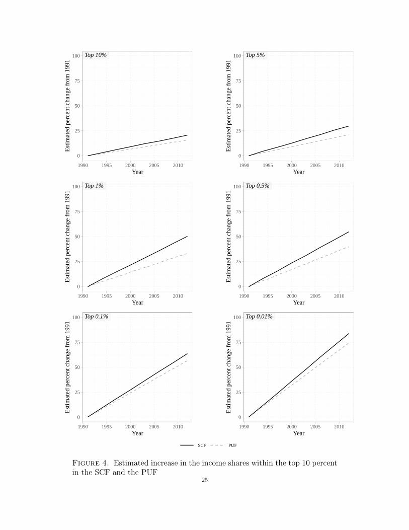
7.6. Long-term trends in income inequality. This section discusses long-term trends in

income inequality. My two main objectives are to compare the estimated trend lines of the

SCF and the PUF and to determine whether an observed increase in top income inequality

between the early 1990s and early 2010s is statistically significant. In this exercise, I use

data from 1991 through 2012 and regress estimated income shares (of the top 10 to the

top 0.01 percent) on a constant and linear time trend using weighted least squares, with

weights defined as reciprocals of squared standard errors.29 As indicated in Figure 4, I

find that both the SCF and the PUF suggest a statistically significant increase in all six

top-decile income shares under consideration (see Table C.5 in Appendix C of the Online

Supplementary Material for the estimation details.). However, the two data sets do not fully

agree with respect to the estimated increase in income shares, with the SCF trend lines being

consistently steeper than those constructed using the PUF. Nevertheless, since the observed

discrepancies are moderate and by no means extensive, the two data sets imply an increase

of comparable magnitude in top income inequality between the early 1990s and early 2012.

7.7. Income inequality and the Great Recession. After discussing the long-term dy-

namics in income inequality, in the present section, I focus on a shorter time horizon before

and after the 2007–2009 Great Recession. Specifically, in Figure 5, I present point estimates

and their 95 percent confidence intervals for income shares of the top 10 percent, constructed

29Note that while the PUF standard error consists only of sampling error, the SCF standard error com-prises both sampling and imputation errors.

24

Top 10%Top 10%Top 10%Top 10%Top 10%Top 10%Top 10%Top 10%

0

25

50

75

100

1990 1995 2000 2005 2010Year

Est

imat

ed p

erce

nt c

hang

e fr

om 1

991

Top 5%Top 5%Top 5%Top 5%Top 5%Top 5%Top 5%Top 5%

0

25

50

75

100

1990 1995 2000 2005 2010Year

Est

imat

ed p

erce

nt c

hang

e fr

om 1

991

Top 1%Top 1%Top 1%Top 1%Top 1%Top 1%Top 1%Top 1%

0

25

50

75

100

1990 1995 2000 2005 2010Year

Est

imat

ed p

erce

nt c

hang

e fr

om 1

991

Top 0.5%Top 0.5%Top 0.5%Top 0.5%Top 0.5%Top 0.5%Top 0.5%Top 0.5%

0

25

50

75

100

1990 1995 2000 2005 2010Year

Est

imat

ed p

erce

nt c

hang

e fr

om 1

991

Top 0.1%Top 0.1%Top 0.1%Top 0.1%Top 0.1%Top 0.1%Top 0.1%Top 0.1%

0

25

50

75

100

1990 1995 2000 2005 2010Year

Est

imat

ed p

erce

nt c

hang

e fr

om 1

991

Top 0.01%Top 0.01%Top 0.01%Top 0.01%Top 0.01%Top 0.01%Top 0.01%Top 0.01%

0

25

50

75

100

1990 1995 2000 2005 2010Year

Est

imat

ed p

erce

nt c

hang

e fr

om 1

991

SCF PUF

Figure 4. Estimated increase in the income shares within the top 10 percentin the SCF and the PUF

25

using the SCF and the PUF between 2006 and 2012. I observe that the PUF estimates

suggest a sharp and statistically significant decrease in incomes shares of the top 10 percent

from 2007 to 2009, followed by a three-year long recovery to pre-recession levels. As noted by

Thompson et al. (2018) “the factors explaining the rise and fall in income concentration are

not fully understood, but some of the most prominent explanations for rising top incomes

highlight the role played by individuals—who may be ‘superstars’ (Rosen, 1981) or ‘rent

seekers’ (Bivens and Mishel, 2013)—whose compensation is relatively volatile from one year

to the next (Bebchuk and Fried, 2003; Kaplan and Rauh, 2013, among others).” By contrast,

the SCF does not support the claim of a statistically significant change in income shares of

the top 10 percent in relation to the impact of the Great Recession. Therefore, while the

SCF can be used to analyze long-term dynamics and detect changes in income shares over

longer-time horizons, it lacks statistical power to determine changes in income inequality

over shorter-time horizons, including recessions and economic expansions.

●

●

●

●

●

●

●

42

43

44

45

46

2006 2008 2010 2012Year

Inco

me

shar

e of

the

top

10

% (

in p

erce

nt) ●●

SCFPUF

Figure 5. Income shares of the top 10 percent before and after the 2007–2009 Great Recession in the SCF and the PUF. Error bars indicate 95 percentconfidence intervals around point estimates

7.8. Regression analysis. Lastly, I investigate whether there exists a statistical link be-

tween the SCF and the PUF. In this exercise, I regress the PUF point estimates on the SCF26

point estimates for each top-decile income share under consideration. As shown in Table

3, my analysis indicates strong correlation between the PUF and the SCF income shares of

the top 10 to the top 0.5 percent.30 This result is of great importance since it opens up the

possibility of merging the two data sets into one, which would result in a superior data set

with plenty of observations (see the PUF) and a rich set of demographic and socio-economic

characteristics (see the SCF).

Table 3. Estimation results from regressing the PUF on the SCF for theincome shares within the top 10 percent

RegressorPUF income share of the top k%

10% 5% 1% 0.5% 0.1% 0.01%

Intercept0.075??? 0.061??? 0.030??? 0.021??? 0.024??? 0.017???

(1.793)??? (1.990)??? (1.486)??? (0.892)??? (1.126)??? (2.086)???

SCF income shareof the top k%

0.817??? 0.772??? 0.763??? 0.789??? 0.633??? 0.321???

(8.204)??? (7.799)??? (5.968)??? (3.837)??? (1.673)??? (0.727)???

R2 0.918 0.910 0.856 0.710 0.318 0.081

This table summarizes estimation results from six unweighted linear regressions of the PUF incomeshares on a constant and the SCF income shares. I report estimated coefficients and t-statisticsin parentheses. “???” denotes statistical significance at the 99 percent significance level.

7.9. Key findings. A natural question is which data set, the SCF survey data or the PUF

sample of tax records, proves more reliable in analyzing top income inequality? My study

suggests that when interested primarily in estimates of top income shares, the PUF is better

than the SCF. However, when interested in top income inequality more broadly defined, the

answer depends on the research question at hand.

The main advantage of using the PUF lies in higher data frequency and more precise esti-

mates.31 As discussed in detail in Section 7.3, the PUF sampling error is five times smaller

than that of the SCF. Moreover, the SCF imputation error, briefly characterized in Section

7.5, introduces an additional and for the earlier years non-negligible layer of uncertainty to

the SCF point estimates, whereas the PUF nonresponse error is likely to be inconsequential.

Consequently, once all sources of error are accounted for, the SCF standard error is likely

to be at least five times larger than that of the PUF. Note that though this study does

not estimate all components of TSE, it provides qualitative evidence suggesting that, once

30For more granular income shares of the top 0.1 and 0.01 percent, the relationship in question is statis-tically insignificant.

31Moreover, as emphasized by Atkinson et al. (2011), tax data are available for longer time horizons andmany more countries than are survey data, which makes it possible to study structural shifts in incomedistributions spanning several decades and to conduct cross-country comparisons.

27

accounted for, measurement error in the SCF is still likely to be much more substantial than

in the PUF.

A natural question is whether more households could be surveyed for the SCF with the

objective of producing more precise estimates of income concentration. Given that the cost

of conducting the 2015 SCF was equal to $18 million, increasing the SCF sample size would

be an expensive undertaking, and therefore, any such decision would require a detail cost-

benefit analysis, which is beyond the scope of the current paper.

Since SCF estimates are considerably less precise than those constructed using the PUF, can

they still be used to draw reliable conclusions regarding top income inequality? My study

suggests that while the SCF can be used to answer most questions regarding the long-term

dynamics in less granular income shares, the data is not well-suited to analyze short-term

horizons or year-to-year changes.

Regarding long-term dynamics, in Section 7.6, I find that both the SCF and the PUF

suggest a statistically significant increase in all of the six top-decile income shares under

consideration. However, as we move from less to more granular income shares, the accuracy

of the SCF point estimates deteriorates (see Section 7.3). Moreover, as discussed in further

detail in Section 7.4, relative increments in CVs in the SCF are much more pronounced than

those in the PUF. Consequently, using the SCF for the estimation of more granular income

shares leads to a greater loss in precision than if we were to use the PUF. Lastly, Section

7.1 shows that the (weighted) number of observations in the SCF above the 99.9 and 99.99

income fractiles is insufficient in both absolute and relative terms, especially when compared

to the large number of observations in the PUF. Therefore, even though the SCF may be

useful for analyzing long-term dynamics in income shares of the top 10 or 5 percent, it should

not be used in studies that focus on the top 0.1 or 0.01 percent.

Yet Saez and Zucman (2016), Bricker et al. (2018), Saez and Zucman (2020b), and others

continue to rely upon the SCF estimates of the most granular income and wealth shares of the

top 0.1 and the top 0.01 percent. In particular, the estimates in question are used as reference

points in assessing income and wealth concentration measures obtained using alternative

data sets and/or different estimation techniques. Most importantly, such comparisons are

done without accounting for the SCF standard error, which affects not only the SCF point

estimates, but foremost, the short- and long-term dynamics in income and wealth inequality.

A notable exception is Kopczuk and Saez (2004) who acknowledge the small number of

observations in the SCF and find the survey data unreliable for the estimation of wealth

shares for groups smaller than the top 0.5 percent.28

Regarding short-term dynamics, I find that large confidence intervals around the SCF point

estimates may falsely suggest lack of a statistically significant increase in income shares

from one SCF survey year to another. For instance, whereas the SCF does not suggest

a statistically significant change in top income shares before, during, and after the 2007–

2009 Great Recession, the PUF clearly illustrates an initial drop (2006–2009) followed by a

statistically significant increase (2009–2012), to at or even above the pre-recession levels.

On the other hand, when it is necessary to control for a wide range of demographic and

socio-economic characteristics or examine the composition of top earners by age, sex, or

marital status, the PUF cannot be used, and instead, one must rely upon the SCF.32 In

order to arrive at credible results using the SCF, it is important to account for the survey’s

small number of observations, and, as such, refrain from estimating very granular income

shares or analyzing small population subgroups. For instance, while I presume the SCF to

accurately estimate the difference in trends in top income inequality between married and

unmarried households, the number of observations is likely insufficient to produce credible

results on married and unmarried households with and without dependents.

An ideal data set for studying top income inequality would comprise a large number of

observations and a rich set of demographic and socio-economic characteristics. Could such

a data set be constructed from a merge of the data from the SCF and the PUF? While the

answer to this question is beyond the scope of the current paper, as shown in Section 7.8,

there exists an explicit statistical link between between the PUF and the SCF, which could

be used in a follow-up research project to analyze how economic factors could impact PUF

through its link with SCF.33

Specifically, combining information from the SCF and the PUF would be particularly ad-

vantageous for studying racial and ethnic income inequality. According to the New York

Times, a black family with a newborn baby has a median household income of $36,300,

which compares to $80,000 for white households.34 Moreover, since COVID-19 is having

disproportionate impact on people of color (blacks have the highest death toll per 100,000,

in comparison to whites, Asians, Latinos, and indigenous Americans)35 we can expect these

longstanding racial and ethnic disparities in income to grow. So far, the Tax Policy Center

32Even in the highly-restricted INSOLE sample data, information on taxpayers’ demographics and socio-economic characteristics is limited to age and sex.

33Moreover, since the PUF is released with a substantial delay when compared to the SCF (the latestavailable data set is from 2012), it is even more critical to statistically link the PUF and the SCF. Whilenaive way would be through regressions, a more sophisticated approach belongs to future research.

34See https://www.nytimes.com/2020/06/09/your-money/race-income-equality.html (accessed on Octo-ber 7, 2020).

35See https://www.apmresearchlab.org/covid/deaths-by-race (accessed on October 7, 2020).29

and the Joint Committee of Taxation used administrative tax records in combination with

the SCF survey data to examine the impact of the 2017 federal corporate tax cut (Trump’s

tax) on racial and ethnic income inequality.36 Given the widening gap in income between

black and white Americans, similar analyses are called for in the context of COVID-19, the

2007–2009 Great Recession, and any other major shock to the post-WWII US economy.

Consequently, this study does not portray the SCF and the PUF as supplements but rather

as complementary data sources that can and should be used interchangeably in order to

best answer a specific research question. However, this is often not possible due to a strictly

limited access to individual-income tax returns, which is only granted to a handful of re-

searchers. For this reason, this paper advocates for a broader access to various sources of

administrative micro-level data (such as the PUF), supporting the calls by Card et al. (2010)

and others.

7.9.1. Conclusion. Regarding top income inequality, I find a statistically significant increase

in all six top-decile income shares under consideration in the twenty-two-year period between

1991 and 2012. Specifically, the weighted least square regression analysis of the PUF esti-

mates suggests an increase in income shares of the top 10, 5, 1, 0.5, 0.1, and 0.01 percent by

16, 21, 33, 40, 56, and 75 percent, respectively. These results are in line with those published

in the related literature, supporting the claim of the long-term trend toward growing income

concentration.

8. Empirical results on wealth shares

My analysis of the wealth shares within the top 10 percent is based on four sets of estimates:

one constructed using the SCF and three constructed using the PUF. The first set of PUF

estimates corresponds to wealth shares estimated under a homogeneity assumption imposed

on all rates of return of the underlying capitalization model, whereas the other two sets

allow for heterogeneous rates of return on taxable interest-bearing assets. In Section 8.1, I

examine the number of observations available for the estimation of top wealth inequality in

the SCF and the PUF. In Sections 8.2–8.6, I discuss point estimates, standard errors, and

the long- and short-term dynamics in top wealth inequality. Finally, Section 8.7 summarizes

my main finding and concludes.

8.1. Number of observations. I start my analysis with a brief description of the total

and weighted number of observations available for the estimation of the six top-decile wealth

shares under consideration in the SCF and the PUF between 1991 and 2012. Since neither of

36See https://www.nytimes.com/2018/10/11/business/trump-tax-cuts-white-americans.html (accessedon October 7, 2020).

30

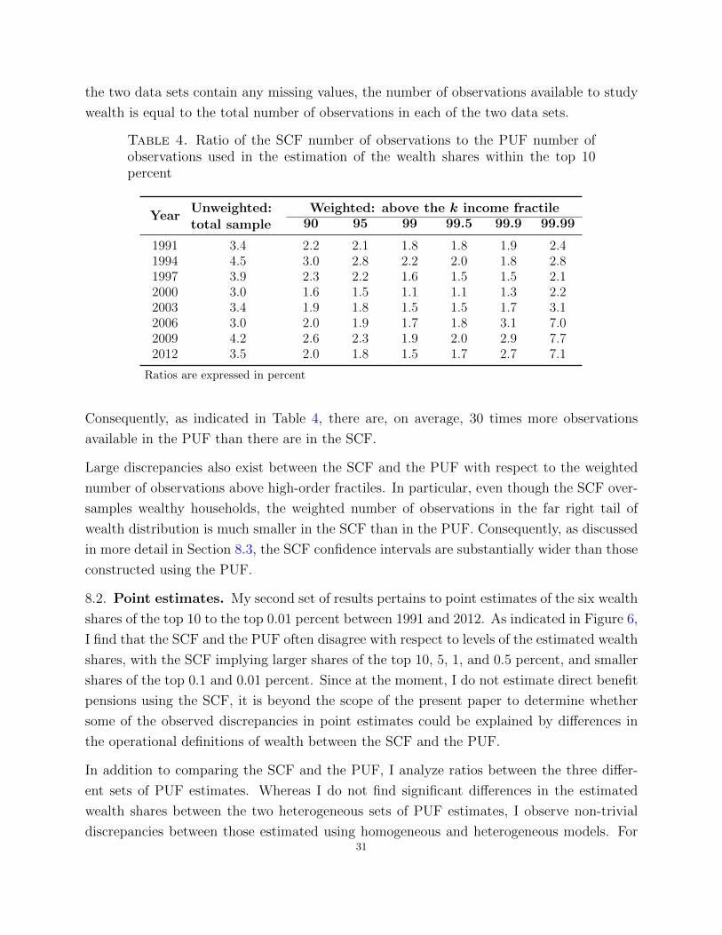
the two data sets contain any missing values, the number of observations available to study

wealth is equal to the total number of observations in each of the two data sets.

Table 4. Ratio of the SCF number of observations to the PUF number ofobservations used in the estimation of the wealth shares within the top 10percent

YearUnweighted:total sample

Weighted: above the k income fractile90 95 99 99.5 99.9 99.99

1991 3.4 2.2 2.1 1.8 1.8 1.9 2.41994 4.5 3.0 2.8 2.2 2.0 1.8 2.81997 3.9 2.3 2.2 1.6 1.5 1.5 2.12000 3.0 1.6 1.5 1.1 1.1 1.3 2.22003 3.4 1.9 1.8 1.5 1.5 1.7 3.12006 3.0 2.0 1.9 1.7 1.8 3.1 7.02009 4.2 2.6 2.3 1.9 2.0 2.9 7.72012 3.5 2.0 1.8 1.5 1.7 2.7 7.1

Ratios are expressed in percent

Consequently, as indicated in Table 4, there are, on average, 30 times more observations

available in the PUF than there are in the SCF.

Large discrepancies also exist between the SCF and the PUF with respect to the weighted

number of observations above high-order fractiles. In particular, even though the SCF over-

samples wealthy households, the weighted number of observations in the far right tail of

wealth distribution is much smaller in the SCF than in the PUF. Consequently, as discussed

in more detail in Section 8.3, the SCF confidence intervals are substantially wider than those

constructed using the PUF.

8.2. Point estimates. My second set of results pertains to point estimates of the six wealth

shares of the top 10 to the top 0.01 percent between 1991 and 2012. As indicated in Figure 6,

I find that the SCF and the PUF often disagree with respect to levels of the estimated wealth

shares, with the SCF implying larger shares of the top 10, 5, 1, and 0.5 percent, and smaller

shares of the top 0.1 and 0.01 percent. Since at the moment, I do not estimate direct benefit

pensions using the SCF, it is beyond the scope of the present paper to determine whether

some of the observed discrepancies in point estimates could be explained by differences in

the operational definitions of wealth between the SCF and the PUF.

In addition to comparing the SCF and the PUF, I analyze ratios between the three differ-

ent sets of PUF estimates. Whereas I do not find significant differences in the estimated

wealth shares between the two heterogeneous sets of PUF estimates, I observe non-trivial

discrepancies between those estimated using homogeneous and heterogeneous models. For31

● ● ● ● ● ● ● ●

●●

●

●●

●

●

●

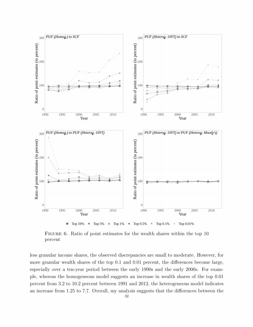
PUF (Homog.) to SCFPUF (Homog.) to SCFPUF (Homog.) to SCFPUF (Homog.) to SCFPUF (Homog.) to SCFPUF (Homog.) to SCFPUF (Homog.) to SCFPUF (Homog.) to SCF

0

100

200

300

1990 1995 2000 2005 2010Year

Rat

io o

f poi

nt e

stim

ates

(in

per

cent

)

● ● ● ● ● ● ● ●

●●

●● ● ●

● ●

PUF (Heterog. 10YT) to SCFPUF (Heterog. 10YT) to SCFPUF (Heterog. 10YT) to SCFPUF (Heterog. 10YT) to SCFPUF (Heterog. 10YT) to SCFPUF (Heterog. 10YT) to SCFPUF (Heterog. 10YT) to SCFPUF (Heterog. 10YT) to SCF

0

100

200

300

1990 1995 2000 2005 2010Year

Rat

io o

f poi

nt e

stim

ates

(in

per

cent

)

●● ● ● ● ● ● ●

●

●●

●● ●

●

●

PUF (Homog.) to PUF (Heterog. 10YT)PUF (Homog.) to PUF (Heterog. 10YT)PUF (Homog.) to PUF (Heterog. 10YT)PUF (Homog.) to PUF (Heterog. 10YT)PUF (Homog.) to PUF (Heterog. 10YT)PUF (Homog.) to PUF (Heterog. 10YT)PUF (Homog.) to PUF (Heterog. 10YT)PUF (Homog.) to PUF (Heterog. 10YT)

0

100

200

300

1990 1995 2000 2005 2010Year

Rat

io o

f poi

nt e

stim

ates

(in

per

cent

)

● ● ● ● ● ● ● ●● ● ● ●

● ● ● ●

PUF (Heterog. 10YT) to PUF (Heterog. Moody's)PUF (Heterog. 10YT) to PUF (Heterog. Moody's)PUF (Heterog. 10YT) to PUF (Heterog. Moody's)PUF (Heterog. 10YT) to PUF (Heterog. Moody's)PUF (Heterog. 10YT) to PUF (Heterog. Moody's)PUF (Heterog. 10YT) to PUF (Heterog. Moody's)PUF (Heterog. 10YT) to PUF (Heterog. Moody's)PUF (Heterog. 10YT) to PUF (Heterog. Moody's)

0

100

200

300

1990 1995 2000 2005 2010Year

Rat

io o

f poi

nt e

stim

ates

(in

per

cent

)

●●●●●● ●●●●●●Top 10% Top 5% Top 1% Top 0.5% Top 0.1% Top 0.01%

Figure 6. Ratio of point estimates for the wealth shares within the top 10percent

less granular income shares, the observed discrepancies are small to moderate. However, for

more granular wealth shares of the top 0.1 and 0.01 percent, the differences become large,

especially over a ten-year period between the early 1990s and the early 2000s. For exam-

ple, whereas the homogeneous model suggests an increase in wealth shares of the top 0.01

percent from 3.2 to 10.2 percent between 1991 and 2012, the heterogeneous model indicates

an increase from 1.25 to 7.7. Overall, my analysis suggests that the differences between the32

● ● ● ● ●

●

●

●●

● ●

●

●

●

●

●

PUF (Homog.) to SCFPUF (Homog.) to SCFPUF (Homog.) to SCFPUF (Homog.) to SCFPUF (Homog.) to SCFPUF (Homog.) to SCFPUF (Homog.) to SCFPUF (Homog.) to SCF

0

40

80

120

1990 1995 2000 2005 2010Year

Rat

io o

f CV

s (in

per

cent

)

● ●●

●

●

●

●

●

● ●

●

●

●

●

●

●

PUF (Heterog. 10YT) to SCFPUF (Heterog. 10YT) to SCFPUF (Heterog. 10YT) to SCFPUF (Heterog. 10YT) to SCFPUF (Heterog. 10YT) to SCFPUF (Heterog. 10YT) to SCFPUF (Heterog. 10YT) to SCFPUF (Heterog. 10YT) to SCF

0

40

80

120

1990 1995 2000 2005 2010Year

Rat

io o

f CV

s (in

per

cent

)

●● ● ●

●●

●●

●

●

●●

● ●

●

●

PUF (Homog.) to PUF (Heterog. 10YT)PUF (Homog.) to PUF (Heterog. 10YT)PUF (Homog.) to PUF (Heterog. 10YT)PUF (Homog.) to PUF (Heterog. 10YT)PUF (Homog.) to PUF (Heterog. 10YT)PUF (Homog.) to PUF (Heterog. 10YT)PUF (Homog.) to PUF (Heterog. 10YT)PUF (Homog.) to PUF (Heterog. 10YT)

0

40

80

120

1990 1995 2000 2005 2010Year

Rat

io o

f CV

s (in

per

cent

)

● ● ●

●

●●

●

●●

●●

● ●

●

●

●

PUF (Heterog. 10YT) to PUF (Heterog. Moody's)PUF (Heterog. 10YT) to PUF (Heterog. Moody's)PUF (Heterog. 10YT) to PUF (Heterog. Moody's)PUF (Heterog. 10YT) to PUF (Heterog. Moody's)PUF (Heterog. 10YT) to PUF (Heterog. Moody's)PUF (Heterog. 10YT) to PUF (Heterog. Moody's)PUF (Heterog. 10YT) to PUF (Heterog. Moody's)PUF (Heterog. 10YT) to PUF (Heterog. Moody's)

0

40

80

120

1990 1995 2000 2005 2010Year

Rat

io o

f CV

s (in

per

cent

)

●●●●●● ●●●●●●Top 10% Top 5% Top 1% Top 0.5% Top 0.1% Top 0.01%

Figure 7. Ratio of CVs for the wealth shares within the top 10 percent

homogeneous and heterogeneous PUF estimates are similar in magnitude to those observed

between the SCF and the PUF. Consequently, except for wealth shares of the top 10 percent,

there is little agreement between the different set of estimates, which makes the analysis of

wealth inequality considerably more challenging than that of income.

8.3. Relative magnitudes of sampling error across data sets. In the present section,

I focus on sampling errors. In particular, I analyze ratios of CVs computed for the six33

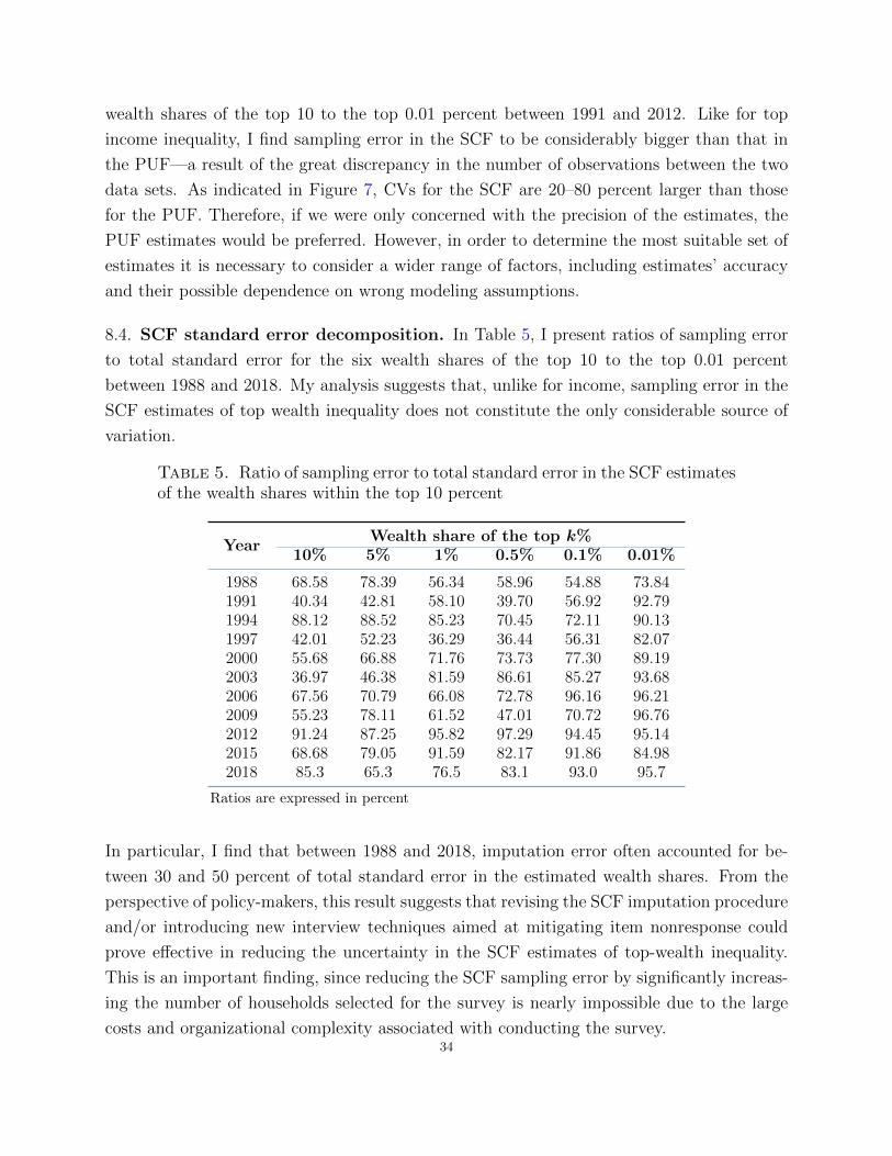
wealth shares of the top 10 to the top 0.01 percent between 1991 and 2012. Like for top

income inequality, I find sampling error in the SCF to be considerably bigger than that in

the PUF—a result of the great discrepancy in the number of observations between the two

data sets. As indicated in Figure 7, CVs for the SCF are 20–80 percent larger than those

for the PUF. Therefore, if we were only concerned with the precision of the estimates, the

PUF estimates would be preferred. However, in order to determine the most suitable set of

estimates it is necessary to consider a wider range of factors, including estimates’ accuracy

and their possible dependence on wrong modeling assumptions.

8.4. SCF standard error decomposition. In Table 5, I present ratios of sampling error

to total standard error for the six wealth shares of the top 10 to the top 0.01 percent

between 1988 and 2018. My analysis suggests that, unlike for income, sampling error in the

SCF estimates of top wealth inequality does not constitute the only considerable source of

variation.

Table 5. Ratio of sampling error to total standard error in the SCF estimatesof the wealth shares within the top 10 percent

YearWealth share of the top k%

10% 5% 1% 0.5% 0.1% 0.01%

1988 68.58 78.39 56.34 58.96 54.88 73.841991 40.34 42.81 58.10 39.70 56.92 92.791994 88.12 88.52 85.23 70.45 72.11 90.131997 42.01 52.23 36.29 36.44 56.31 82.072000 55.68 66.88 71.76 73.73 77.30 89.192003 36.97 46.38 81.59 86.61 85.27 93.682006 67.56 70.79 66.08 72.78 96.16 96.212009 55.23 78.11 61.52 47.01 70.72 96.762012 91.24 87.25 95.82 97.29 94.45 95.142015 68.68 79.05 91.59 82.17 91.86 84.982018 85.3 65.3 76.5 83.1 93.0 95.7

Ratios are expressed in percent

In particular, I find that between 1988 and 2018, imputation error often accounted for be-

tween 30 and 50 percent of total standard error in the estimated wealth shares. From the

perspective of policy-makers, this result suggests that revising the SCF imputation procedure

and/or introducing new interview techniques aimed at mitigating item nonresponse could

prove effective in reducing the uncertainty in the SCF estimates of top-wealth inequality.

This is an important finding, since reducing the SCF sampling error by significantly increas-

ing the number of households selected for the survey is nearly impossible due to the large

costs and organizational complexity associated with conducting the survey.34

Top 10%Top 10%Top 10%Top 10%Top 10%Top 10%Top 10%Top 10%

0

5

10

15

20

1990 1995 2000 2005 2010Year

Est

imat

ed p

erce

nt c

hang

e fr

om 1

991

Top 5%Top 5%Top 5%Top 5%Top 5%Top 5%Top 5%Top 5%

0

5

10

15

20

1990 1995 2000 2005 2010Year

Est

imat

ed p

erce

nt c

hang

e fr

om 1

991

Top 1%Top 1%Top 1%Top 1%Top 1%Top 1%Top 1%Top 1%

0

20

40

60

1990 1995 2000 2005 2010Year

Est

imat

ed p

erce

nt c

hang

e fr

om 1

991

Top 0.5%Top 0.5%Top 0.5%Top 0.5%Top 0.5%Top 0.5%Top 0.5%Top 0.5%

0

20

40

60

1990 1995 2000 2005 2010Year

Est

imat

ed p

erce

nt c

hang

e fr

om 1

991

Top 0.1%Top 0.1%Top 0.1%Top 0.1%Top 0.1%Top 0.1%Top 0.1%Top 0.1%

0

100

200

300

400

1990 1995 2000 2005 2010Year

Est

imat

ed p

erce

nt c

hang

e fr

om 1

991

Top 0.01%Top 0.01%Top 0.01%Top 0.01%Top 0.01%Top 0.01%Top 0.01%Top 0.01%

0

100

200

300

400

1990 1995 2000 2005 2010Year

Est

imat

ed p

erce

nt c

hang

e fr

om 1

991

SCF PUF (Homog.) PUF (Heterog. 10YT) PUF (Heterog. Moody's)

Figure 8. Estimated increase in the wealth shares within the top 10 percentin the SCF and the PUF

35

8.5. Long-term dynamics. In order to analyze long-term dynamics in wealth inequality

between 1991 and 2012, I estimate weighted linear regressions of top-decile wealth shares

on a constant and linear time trend. As illustrated in Figure 8, the SCF regression results

support the claim of a statistically significant increase in three out of the six wealth shares

under consideration (see Table C.6 in Appendix C of the Online Supplementary Material for

the estimation details). I find a statistically significant increase in the wealth shares of the

top 10 and the top 5 percent at the 1 percent significance level, and in the wealth shares

of the top 1 percent at the 10 percent significance level. The PUF estimates, on the other

hand, suggest a statistically significant increase in all of the six top-decile wealth shares

under consideration, irrespective of the assumption imposed on the rate of return of taxable

interest-bearing assets. However, there exist considerable differences in the estimated trend

lines between the homogeneous and heterogeneous sets of estimates. For the wealth shares

of the top 10 and 5 percent, the homogeneous model suggests a greater increase in inequality

between 1991 and 2012 than the heterogeneous model. Yet for the wealth shares of the top

0.1 and 0.01 percent the opposite is true: the heterogeneous model indicates a much more

pronounced increase than the homogeneous model. In particular, the estimated percent

change in the wealth shares of the top 0.01 percent from 1991 to 2012 exceeds 300 percent

for the heterogeneous model while being equal to over 100 percent for the homogeneous

model. Therefore, without taking a strong stance on what model better describes the state

of the economy, the PUF estimates remain inconclusive with respect to the magnitude by

which the top wealth inequality has increased.

8.6. Wealth inequality and the Great Recession. In the present section, I discuss

the impact of the 2007–2009 Great Recession on wealth inequality, with the main focus on

wealth shares of the top 10 percent between 2006 and 2012. As illustrated in Figure 9, I

find considerable differences between the homogeneous and heterogeneous PUF estimates.

Specifically, whereas homogeneous estimates had been steadily increasing in the aftermath

of the Great Recession, heterogeneous estimates came to near standstill once the recession

ended. In other words, the two sets of estimates lead to drastically different conclusions

regarding the short-term dynamics in top wealth inequality. One set of estimates suggests

a statistically significant increase of 2 percentage points between 2009 and 2012, whereas

the other set implies no statistically significant change since the recession came to an end

in 2009. Therefore, with reference to Section 8.5, I find the PUF estimates inconclusive not

only in relation to the long-term dynamics in top wealth inequality, but also when examining

shorter-time horizons and times of rapid economic changes, such as the 2007–2009 Great

Recession.36

●

●

●

● ●●

●

●

●

●

●

●

●

●

68

70

72

74

76

2006 2008 2010 2012Year

Wea

lth s

hare

of t

he to

p 1

0 %

(in

per

cent

) ●●●●

●●●●

SCFPUF (Homog.)PUF (Heterog. 10YT)PUF (Heterog. Moody's)

Figure 9. Wealth shares of the top 10 percent before and after the 2007–2009Great Recession measured in the SCF and the PUF. Error bars indicate 95percent confidence intervals around point estimates

8.7. Key findings. My analysis suggests that the PUF estimates of top wealth inequality

are largely inconclusive—a result of substantial differences in the estimates resulting from

the set of assumptions imposed on the underlying capitalization model.

As indicated in Section 8.2, I find non-trivial differences in the PUF point estimates obtained

under the homogeneity assumption and those computed using heterogeneous rates of return

on taxable interest-bearing assets. In addition to disparities in point estimates, the two sets

of estimates differ with respect to short- and long-run trends in top wealth inequality. First,

regarding the long-term dynamics, the estimated trend lines lead to different conclusions

regarding the severity of the ongoing crisis linked to rising inequality. Second, regarding the

short-term dynamics, I find that whereas the homogeneous estimates support the claim of

an increase in wealth inequality following the 2007–2009 Great Recession, the heterogeneous

estimates do not indicate a statistically significant change.

Assuming different rates of return leads to considerably different dynamics in top wealth

inequality. Then, since the assumptions matter, a natural question is what rates of return37

should we be considering for each of the asset classes under consideration? Should they be

mostly homo- or heterogeneous? Should we allow them to vary by income or wealth per-

centile? Should they depend on portfolio composition or regional macroeconomic conditions?

In this paper, following Bricker et al. (2018), I consider a heterogeneous rate of return on only

one class of assets, where I impose a hard, and rather unrealistic, cut-off between high and

low rates of return. Therefore, another important question is whether a different and more

realistic set of assumptions would result in distinct estimates of top wealth inequality. Based

on the extent to which the PUF estimates obtained under the homogeneity assumption and

those computed using heterogeneous rates of return on taxable interest-bearing assets differ,

I presume the resulting estimates would be considerably different from those currently ob-

tained. This presumption is line with Kopczuk and Saez (2004), who, among many others,

expressed concerns about the estimation of wealth using tax-based income data, resulting

from “substantial and unobservable heterogeneity in the returns of many assets, especially

corporate stock.”

Since the PUF estimates of top wealth inequality are functions of numerous assumptions

imposed on the underlying capitalization model, is the SCF a better alternative? My anal-

ysis suggests that for the less granular income shares of the top 10 to the top 0.5 percent

the SCF appears more reliable. This results mainly from the fact that the SCF measures

wealth, whereas the PUF infers wealth from data on income. However, using the SCF for

the estimation of top wealth shares has its own limitations resulting from a small number

of observations and large confidence intervals. Therefore, whereas the SCF can be used ef-

fectively to analyze the less granular wealth shares of the top 10 to the top 0.5 percent, the

data remain inadequate to get a realistic picture of the wealth shares of the top 0.1 and 0.01

percent.37

It is important to note that while resolving the problem of the large standard errors in the

SCF would require making changes to the survey design and/or the SCF imputation pro-

cedure, future research could focus on refining the Saez and Zucman (2016)’s capitalization

model, with the objective of producing more reliable estimates of wealth inequality using

the PUF. A significant research effort has been already undertaken by Smith et al. (2019)

and Saez and Zucman (2020a,b), adding to our understanding of the numerous advantages

and disadvantages embedded in studying wealth inequality using capitalization methods.

Since both the SCF survey data and the PUF individual-income tax returns pose major

challenges for the estimation of top wealth inequality in the US, this paper supports Saez

37The wealth shares of the top 10 to the top 0.5 percent constructed using the SCF can be further refinedby adding the wealth of the Forbes 400 wealthiest Americans and the value of direct benefit pensions as inBricker et al. (2016).

38

and Zucman (2020b) in calling for “more and improved statistics on inequality.” The authors

further emphasize that “we could and should do better to measure US wealth inequality than

rely on a triennial survey of 6,200 families (the Survey of Consumer Finances) or indirectly

infer asset ownership based on income flows (the capitalization method).”

8.7.1. Conclusions. Regarding the twenty-two year period between 1991 and 2012, my anal-

ysis suggests a statistically significant increase in three out of the six wealth shares under

consideration. Specifically, the weighted least square regression analysis of the SCF esti-

mates suggests a statistically significant increase in wealth shares of the top 10, 5 and 1

percent by 8.4, 8.0, and 3.3 percentage points, respectively, and an insignificant increase in

wealth shares of the top 0.5 percent. Since, as indicated above, neither the SCF nor the PUF

proves credible to analyze more granular wealth shares of the top 0.1 and 0.01 percent, this

study does not draw any conclusions related to top wealth inequality above the 99.5 wealth

fractile. Lastly, my study does not support Saez and Zucman (2016)’s conclusion related to

a decline in the wealth shares of the top 10 less the top 1 percent (i.e., those with wealth

above the 90 wealth percentile but below the 99 wealth percentile). Instead, I find that the

estimated change in the wealth shares of the top 10 percent between 1991 and 2012 exceeds

the estimated change in the wealth shares of the top 1 percent by 2.5 percentage points, a

finding that contradicts the claim of rising wealth inequality among the richest.

9. Structural exercise

In the following, I investigate how the SCF and the PUF data-driven errors in estimates

of top income inequality affect outcomes of structural macroeconomic models. In Section

9.1, I introduce the theoretical foundation of my study, which is the augmented random

growth model with type-dependence proposed by Gabaix et al. (2016). Next, in Section 9.2,

I discuss details of my calibration strategy that, in contrast to the default approach, involves

multiple model calibrations, each time to a different value of the calibration target randomly

drawn from the estimated 95 percent confidence interval. Finally, in Section 9.3, I present

the results of my structural exercise, and conclude on how data-driven errors in calibration

targets may affect outcomes of macroeconomic and policy-oriented studies more generally.

9.1. Model. Consider a continuum of workers, where each worker i is either high- or low-

type, with high-type workers having higher mean growth rate of income than low-type work-

ers. Workers enter the labor market as high-types with probability θ and as low-types with

probability 1 − θ. Whereas no worker of low-type can ever become a high-type, high-type

workers do switch to a low-type with probability α. Since a low-type is an absorbing state,39

high-type workers can switch to a low-type at most once in their life-time. Moreover, work-

ers retire at rate δ and are replaced by new labor entrants with wages drawn from a known

distribution ψ.

Next, let xit denote a natural logarithm of income of worker i of type j at time t, and let

the dynamics of xit be given by a type-dependent random growth model as in Gabaix et al.

(2016):

dxit = µjdt+ σjdZit + Injection−Death, j = {H,L} ,(22)

where Zit is a standard Brownian motion, µj and σ2j are type-dependent mean and variance

of growth rate of log income, and where H and L are shorthand notations for high- and

low-types, respectively.

Moreover, assume that the stationary distribution of log income has a Pareto tail,

P (xit > x) ∼ Ce−ξx,(23)

where C is a constant and ξ > 0 is a power law exponent given by

ξ =−µH +

√µ2H + 2σ2

H (δ − α)

σ2H

.(24)

Finally, impose that the economy is in a Pareto steady state with σH = 0.15, α = 1/6, and

δ = 1/30, and assume that µH is calibrated from a one-to-one-mapping between the inverse

of the power law exponent, say η, and the empirical ratio of two, top-decile income shares:

η =1

ξ= 1 + log10

(p(k/10)pk

).(25)

9.2. Calibration. Unlike Gabaix et al. (2016), where the authors consider a single value of

the inverse of the power law exponent, η, I calibrate the model to multiple values of η drawn

from a 95 percent confidence interval around the η point estimate. In particular, I conduct

B = 100 random draws, where for each drawn value of η, I solve the model for the transition

dynamics to a new steady state.

Gabaix et al. (2016) compute a point estimate of η using data on top income shares from

the World Income Database (WID), whereas this paper’s focus is on the SCF and the PUF.

Moreover, the authors calibrate the model to the 1973 WID, whereas the SCF and the PUF

data considered in this analysis start in 1988 and 1991, respectively. An obvious solution to

this problem would be to estimate η using the 1988 SCF and/or the 1991 PUF. However,

this strategy would not allow me to directly compare my results to those in Gabaix et al.

(2016), since I would be effectively investigating transition dynamics over a different time40

horizon: 1988–2065 (or 1991–2068) versus 1973–2050. Moreover, it would likely require me

to consider a different magnitude of the shock and result in changes to the model parameters

describing the initial Pareto steady state. Instead, I directly build upon the exercise in

Gabaix et al. (2016) at the cost of making two assumptions regarding hypothetical values of

the SCF and the PUF estimates of η in 1973.

Assumption 1 : Let ηSCF,1973 and ηPUF,1973 denote the SCF and the PUF point estimates of η

in 1973, and assume that ηSCF,1973 and ηPUF,1973 are equal to the Gabaix et al. (2016)’s point

estimate of η obtained using the WID, say ηWID,1973:

ηSCF,1973 = ηPUF,1973 = ηWID,1973 = 0.39.(26)

Assumption 2 : Let CVSCF,1973 and CVSCF,1988 denote CVs for the SCF estimates of η in

1973 and 1988, and let CVPUF,1973 and CVPUF,1991 denote CVs for the PUF estimates of η

in 1973 and 1991. In the following, I assume the same CVs for the SCF and the PUF point

estimates of η between the early 1970s and the early 1990s,

CVSCF,1973 = CVSCF,1988 and CVPUF,1973 = CVPUF,1991.(27)

Whereas the first assumption guarantees a direct comparison with Gabaix et al. (2016), the

second conjecture provides me with conservative estimates of the SCF and the PUF standard

errors in η1973.38

In the first step, I compute the point estimates and standard errors of η using the 1988 SCF

and the 1991 PUF. For the SCF, I find ηSCF,1988 = 0.56 and SE (ηSCF,1988) = 0.03, which

results in CVSCF,1988 = 0.054; for the PUF, I find ηPUF,1991 = 0.51 and SE (ηPUF,1991) = 0.001,

which results in CVPUF,1991 = 0.003.

In the second step, I use Assumptions 1 and 2 to compute the standard errors in the SCF

and the PUF estimates of η in 1973:

SE (ηSCF,1973) = CVSCF,1973 × ηSCF,1973 = 0.023(28)

SE (ηPUF,1973) = CVPUF,1973 × ηPUF,1973 = 0.001.(29)

Having estimated SE (ηSCF,1973) and SE (ηPUF,1973), I construct 95 percent confidence intervals

around ηSCF,1973 and ηPUF,1973. For the SCF, the 95 percent confidence interval is given by

[0.36, 0.45]; for the PUF, the 95 percent confidence interval is given by [0.40, 0.41].

38The estimates are conservative since it is likely that the standard errors in the SCF and the PUFestimates of η would have substantially decreased over the twenty-year period between the early 1970s andthe early 1990s.

41

In the third and final step of my analysis, I conduct B = 100 random draws from [0.36, 0.45]

and [0.40, 0.41], where for each drawn value of η, I solve for the model’s transition dynamics

to a new steady state. For each of the two data sets, this exercise results in B = 100

different transition dynamics to a new steady state, where the observed variability in the

model’s outcomes is driven solely by the underlying uncertainty in the estimate of η.

In addition to the uncertainty in the estimate of η, the model is subject to errors arising

from inaccurately assumed values of the remaining model parameters. In the following, I

focus on σH , which Gabaix et al. (2016) set equal to 0.15, while pointing out that σH = 0.15

is a conservative estimate since “the growth rates of parts of the population may be much

more volatile (think of startups).” While an ideal way to account for this additional layer

of uncertainty would be to estimate σH from the data and, then calibrate the model to a 95

percent confidence interval around the point estimate of σH , I leave this approach for future

research. In this paper, I consider a simpler exercise, in which I assume a set of possible

values of σH given by {0.15, 0.175, 0.2}. Note that this set is constructed in accordance with

the Gabaix et al. (2016)’s presumption that the growth rate of log income among high types

is likely to exceed 0.15. Then, for each value of σH and for each of the two data sets under

consideration, I calibrate the model B = 100 times, each time using a different value of η

randomly drawn from a 95 percent confidence interval around the η’s point estimate. This

approach allows me to construct a “feasible region” of the model’s transition dynamics to

a new steady state while incorporating uncertainties arising from data-driven errors in two

out of the six model’s parameters.

9.3. Results. In the following, I discuss two sets of results. First, I analyze the transition

dynamics accounting only for the variation in the calibration target η. Then, I introduce an

additional layer of uncertainty and repeat my analysis for different values of σH , a parameter

that governs the volatility of the growth rate of log income among high types.

9.3.1. Varying η. My first set of results shows that data-driven errors in estimates of key

macroeconomic aggregates impact outcomes of not only empirical but also structural anal-

ysis. Errors in calibration targets are carried over through the model and come to affect all

outcomes of interest, including transition dynamics and the speed of convergence to a new

steady state. Therefore, I find that having precise estimates of calibration targets critical for

producing precise outcomes of structural analysis. This becomes evident when comparing

transition dynamics to a new steady state produced by the exact same model differing, only

with respect to the level of uncertainty surrounding a single calibration target. As indicated

in Figure 10, the PUF estimate of η has a negligible standard error, which results in a pre-

cise estimation of the model’s dynamics to a new steady state. The SCF estimate of η, on42

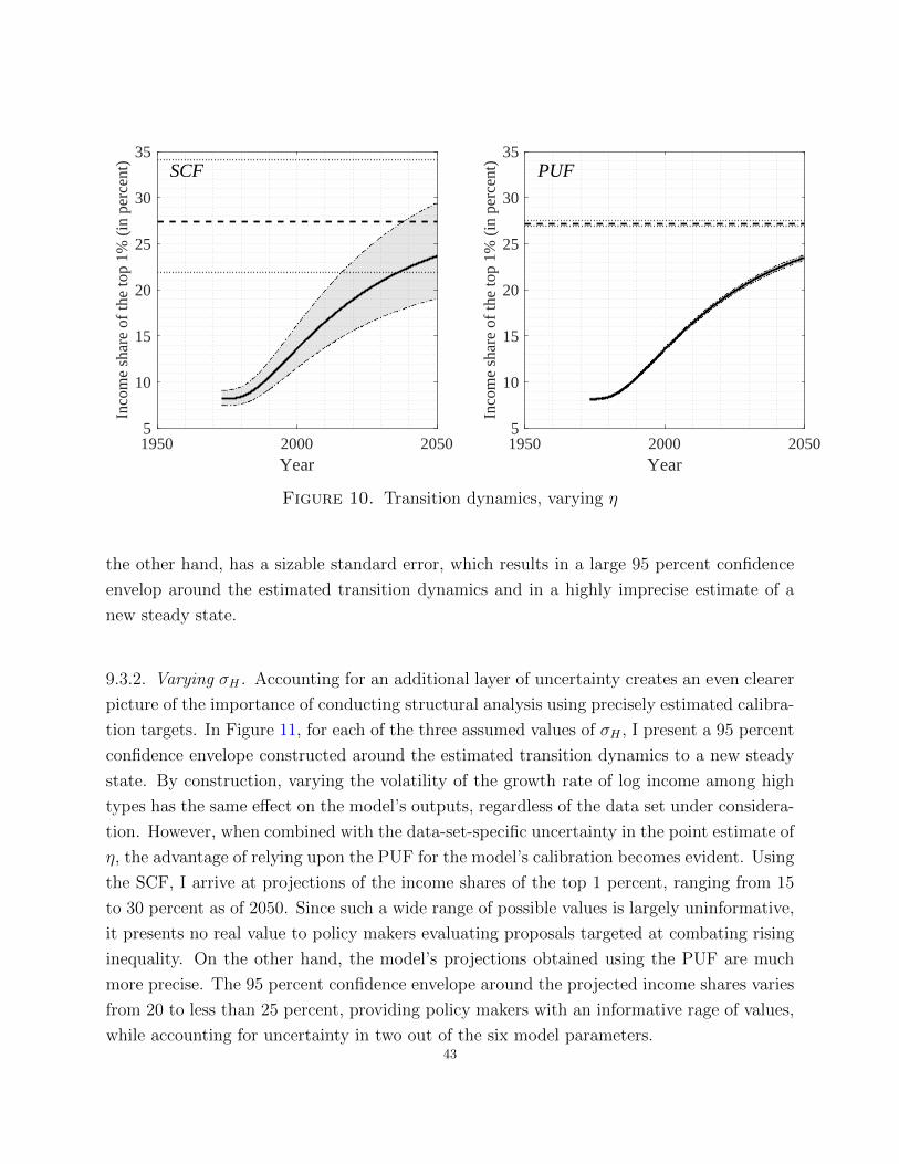
SCF

1950 2000 2050Year

5

10

15

20

25

30

35

Inco

me

shar

e of

the

top

1% (

in p

erce

nt)

PUF

1950 2000 2050Year

5

10

15

20

25

30

35

Inco

me

shar

e of

the

top

1% (

in p

erce

nt)

Figure 10. Transition dynamics, varying η

the other hand, has a sizable standard error, which results in a large 95 percent confidence

envelop around the estimated transition dynamics and in a highly imprecise estimate of a

new steady state.

9.3.2. Varying σH . Accounting for an additional layer of uncertainty creates an even clearer

picture of the importance of conducting structural analysis using precisely estimated calibra-

tion targets. In Figure 11, for each of the three assumed values of σH , I present a 95 percent

confidence envelope constructed around the estimated transition dynamics to a new steady

state. By construction, varying the volatility of the growth rate of log income among high

types has the same effect on the model’s outputs, regardless of the data set under considera-

tion. However, when combined with the data-set-specific uncertainty in the point estimate of

η, the advantage of relying upon the PUF for the model’s calibration becomes evident. Using

the SCF, I arrive at projections of the income shares of the top 1 percent, ranging from 15

to 30 percent as of 2050. Since such a wide range of possible values is largely uninformative,

it presents no real value to policy makers evaluating proposals targeted at combating rising

inequality. On the other hand, the model’s projections obtained using the PUF are much

more precise. The 95 percent confidence envelope around the projected income shares varies

from 20 to less than 25 percent, providing policy makers with an informative rage of values,

while accounting for uncertainty in two out of the six model parameters.43

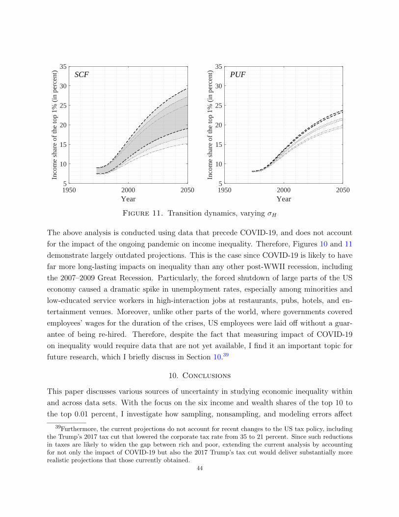
SCF

1950 2000 2050Year

5

10

15

20

25

30

35

Inco

me

shar

e of

the

top

1% (

in p

erce

nt)

PUF

1950 2000 2050Year

5

10

15

20

25

30

35

Inco

me

shar

e of

the

top

1% (

in p

erce

nt)

Figure 11. Transition dynamics, varying σH

The above analysis is conducted using data that precede COVID-19, and does not account

for the impact of the ongoing pandemic on income inequality. Therefore, Figures 10 and 11

demonstrate largely outdated projections. This is the case since COVID-19 is likely to have

far more long-lasting impacts on inequality than any other post-WWII recession, including

the 2007–2009 Great Recession. Particularly, the forced shutdown of large parts of the US

economy caused a dramatic spike in unemployment rates, especially among minorities and

low-educated service workers in high-interaction jobs at restaurants, pubs, hotels, and en-

tertainment venues. Moreover, unlike other parts of the world, where governments covered

employees’ wages for the duration of the crises, US employees were laid off without a guar-

antee of being re-hired. Therefore, despite the fact that measuring impact of COVID-19

on inequality would require data that are not yet available, I find it an important topic for

future research, which I briefly discuss in Section 10.39

10. Conclusions

This paper discusses various sources of uncertainty in studying economic inequality within

and across data sets. With the focus on the six income and wealth shares of the top 10 to

the top 0.01 percent, I investigate how sampling, nonsampling, and modeling errors affect

39Furthermore, the current projections do not account for recent changes to the US tax policy, includingthe Trump’s 2017 tax cut that lowered the corporate tax rate from 35 to 21 percent. Since such reductionsin taxes are likely to widen the gap between rich and poor, extending the current analysis by accountingfor not only the impact of COVID-19 but also the 2017 Trump’s tax cut would deliver substantially morerealistic projections that those currently obtained.

44

outcomes of empirical analysis conducted using the SCF and the PUF. Regarding income

inequality, I find that the PUF estimates are substantially better than the SCF estimates,

and consequently, whenever possible, should be relied upon for both empirical and structural

analysis. On the other hand, for top wealth inequality, neither of the two data sets can be

used without caution. Regarding wealth shares of the top 10 to the top 0.5 percent, I find the

SCF estimates more reliable—a result of unexpected and yet-to-be-accounted-for differences

among the PUF estimates that arise from varying assumptions imposed on the underlying

capitalization model. However, for the more granular wealth shares of the top 0.1 and 0.01

percent, neither of the two data sets proves credible. The PUF estimates lead to different

conclusions depending on which capitalization model one applies, while the SCF estimates

are unreliable as a result of the very sparse number of observations in the far right tail of

wealth distribution.

In addition, using the random growth model of income from Gabaix et al. (2016), I illustrate

how data-driven errors in calibration targets affect the outcomes of structural macroeconomic

models. All in all, I find that in order for a structural analysis to be both conclusive and

informative, it is necessary to rely upon precisely estimated calibration targets. As shown in

Section 9, large uncertainties in the SCF estimates result in wide confidence intervals around

the transition dynamics of the income shares of the top 1 percent, whereas small standard

errors in the PUF estimates lead to estimates with negligible levels of uncertainty.

Regarding future research, one could extend my analysis by estimating the SCF measurement

error, with the main focus on errors arising in the survey response process as described in

Groves et al. (2009). Since other sources of error are either already accounted for in the

present paper or shown to be fairly marginal, computing measurement error would allow

estimation of an upper bound on the SCF total standard error.

Another potentially promising avenue for future research is centered around my structural

exercise. Since my analysis does not account for the impact of COVID-19, the generated

projections of income shares of the top 1 percent until 2050 are largely outdated. This

is the case since data-driven errors in calibration targets are most likely to be of second

order of importance relative to a COVID-19 shock. Since post COVID-19 data will not be

available until 2023 (the expected release date of the 2021 SCF), I plan on implementing

a “hypothetical” COVID-19-recession shock in the model. Specifically, I intend to create

a hypothetical scenario whereby the impact of COVID-19 is equivalent to or greater than

that of the 2007–2009 Great Recession. Because of the severity of the ongoing pandemic

and its uneven impact on US society, I expect the COVID-19 shock to have substantial45

and long-lasting repercussions on inequality, even when compared to those of the Great

Recession.

Next, since, in its present form, the PUF does not provide any information on taxpayers’

demographic and socio-economic characteristics, I plan to design an imputation procedure

that would allow me to embed the SCF within the PUF. This would result in a novel data set

containing as many observations as in the PUF as well as a broad range of demographic and

socio-economic characteristics, which would be imputed from the SCF. With such a rich data

set containing numerous potential control variables, one could answer questions on income

inequality that currently cannot be addressed using the SCF or the PUF individually. For

illustration, consider a problem of examining income inequality among young individuals,

the working-age population, and retirees. The lack of information on age in the PUF and

a small number of observations in the SCF concerning various population subgroups would

make conducting such an analysis virtually impossible.

Finally, while producing better estimates of wealth inequality using the SCF would require

modifying the SCF imputation procedure, introducing new interview techniques aimed at

reducing item nonresponse, and/or increasing the sample size, the PUF estimates could be

improved upon without changes to sampling and/or editing processes. Specifically, future

research could focus on refining Saez and Zucman (2016)’s capitalization model by allowing

for more heterogeneity in the estimated rates of return or conducting a more thorough

analysis of the model’s vulnerability to underlying modeling assumptions.

References

Atkinson, Anthony B., Thomas Piketty, and Emmanuel Saez, “Top incomes in the longrun of history,” Journal of Economic Literature, 2011, 49 (1), 3–71.

Bebchuk, Lucian Arye and Jesse M. Fried, “Executive compensation as an agency problem,”Journal of Economic Perspective, 2003, 17 (3), 71–92.

Biemer, Paul and Lars Lyberg, Introduction to survey quality, Hoboken, New Jersey: JohnWiley & Sons, 2003.

Bivens, Josh and Lawrence Mishel, “The pay of corporate executives and financial professionalsas evidence of rents in top 1 percent incomes,” Journal of Economic Perspective, 2013, 27 (3),57–78.

Bricker, Jesse, Alice Henriques, and Peter Hansen, “How much has wealth concentrationgrown in the United States? A re-examination of data from 2001-2013,” Finance and EconomicsDiscussion Series, 2018, 2018-024, 1–52.

, , Jacob Krimmel, and John Sabelhaus, “Measuring income and wealth atthe top using administrative and survey data,” Brookings Papers on Economic Activity, 2016,Spring, 261–331.

46

Bryant, Victoria L., John L. Czajka, Georgia Ivsin, and Jim Nunns, “Design changesto the SOI Public Use File (PUF),” Prepared for the“New Resources for Microdata-Based TaxAnalysis” Session of the 107th Annual Conference on Taxation, National Tax Association SantaFe, New Mexico, November 15, 2014, pp. 1–19.

Card, David, Raj Chetty, Martin Feldstein, and Emmanuel Saez, “Expanding access toadministrative data for research in the United States,” NSF SBE 2020 White Paper, NationalScience Foundation Directorate of Social, Behavioral, and Economic Sciences, Arlington, VA,2010.

Czajka, John L., Brendan Kirwan, and Amang Sukasih, “An assessment of the need for aredesign of the Statistics of Income Individual Tax Sample,” Mathematica Policy Research, 2014,pp. 1–95.

David, Herbert A. and Haikady N. Nagaraja, Order Statistics, Third Edition, New York–Chichester–Brisbane–Toronto–Singapore: Hoboken, 2003.

Gabaix, Xavier, Jean-Michel Lasry, Pierre-Louis Lions, and Benjamin Moll, “The dy-namics of inequality,” Econometrica, 2016, 84 (6), 2071–2111.

Groen, Jeffrey A., “Sources of error in survey and administrative sata: The importance ofreporting procedures,” Journal of Official Statistics, 2012, 28 (2), 173–198.

Groves, Robert M., Floyd F. Fowler, Mick P. Couper, James M. Lepkowski, EleanorSinger, and Roger Tourangeau, Survey methodology, Hoboken, New Jersey: John Wiley &Sons, 2009.

Hall, Peter, “On the number of bootstrap simulations required to construct a confidence interval,”Journal of Economic Literature, 1986, 14 (4), 1453–1462.

Kaplan, Steven N. and Joshua Rauh, “It’s the market: The broad-based rise in the return totop talent,” Journal of Economic Perspective, 2013, 27 (3), 35–56.

Kennickell, Arthur B., “Consistent weight design for the 1989, 1992, and 1995 SCFs, and thedistribution of wealth,” Working Paper of the Board of Governors of the Federal Reseve System,1997.

, “Multiple imputation in the Survey of Consumer Finances,” Working Paper of the Boardof Governors of the Federal Reseve System, 1998, pp. 1–9.

, “Revisions of the variance estimation procedure for the SCF,” Working Paper of theBoard of Governors of the Federal Reseve System, 2000.

, “The role of over-sampling of the wealthy in the Survey of Consumer Finances,” IrvingFisher Committee Bulletin, 2008, 28.

Kopczuk, Wojciech, “What do we know about the evolution of top wealth shares in the UnitedStates?,” Journal of Economic Perspectives, 2015, 29 (1), 47–66.

and Emmanuel Saez, “Top wealth shares in the United States, 1916–2000: Evidencefrom estate tax records,” National Tax Journal, 2004, 57 (2).

Piketty, Thomas and Emmanuel Saez, “Income inequality in the United States, 1913-1998,”Quarterly Journal of Economics, 2003, 118 (1), 1–39.

47

Reynolds, Alan P., Graeme Richards, Beatriz de la Iglesia, and Victor J. Rayward-Smith, “Clustering rules: A comparison of partitioning and hierarchical clustering algorithms,”Journal of Mathematical Modelling and Algorithms, 1992, 5, 475–504.

Rosen, Sherwin, “The Economics of superstars,” American Economic Review, 1981, 71 (5), 845–858.

Rubin, Donald B., Multiple imputation for nonresponse in surveys, New York–Chichester–Brisbane–Toronto–Singapore: John Wiley & Sons, 1987.

Sabelhaus, John and Alice Henriques Volz, “Are disappearing employer pensions contributingto rising wealth inequality?,” FEDS Notes. Washington: Board of Governors of the FederalReserve System, 2019.

Saez, Emmanuel, “Income and wealth inequality: Evidence and policy Implications,” Contem-porary Economic Policy, 2017, 35 (1).

and Gabriel Zucman, “Wealth Inequality in the United States since 1913: Evidencefrom capitalized tax income data,” Journal of Economic Literature, 2016, 131 (2), 519–578.

and , The triumph of injustice, New York: W. W. Norton & Company, 2019.

and , “Comments on Smith, Zidar and Zwick (2019),” Working Paper, 2020.

and , “Trends in US income and wealth inequality: Revisings after the revision-ists,” Working Paper, 2020.

Smith, Matthew, Owen Zidar, and Eric Zwick, “Top wealth in America: New estimates andimplications for taxing the rich,” Working Paper, 2019.

Thompson, Jeffrey, Michael Parisi, and Jesse Bricker, “Top income concentration andvolatility,” Finance and Economics Discussion Series 2018-010. Washington: Board of Gover-nors of the Federal Reserve System, 2018.

48